NICER-SLAM: Neural Implicit Scene Encoding for RGB SLAM

Abstract

Neural implicit representations have recently become popular in simultaneous localization and mapping (SLAM), especially in dense visual SLAM. However, previous works in this direction either rely on RGB-D sensors, or require a separate monocular SLAM approach for camera tracking and do not produce high-fidelity dense 3D scene reconstruction. In this paper, we present NICER-SLAM, a dense RGB SLAM system that simultaneously optimizes for camera poses and a hierarchical neural implicit map representation, which also allows for high-quality novel view synthesis. To facilitate the optimization process for mapping, we integrate additional supervision signals including easy-to-obtain monocular geometric cues and optical flow, and also introduce a simple warping loss to further enforce geometry consistency. Moreover, to further boost performance in complicated indoor scenes, we also propose a local adaptive transformation from signed distance functions (SDFs) to density in the volume rendering equation. On both synthetic and real-world datasets we demonstrate strong performance in dense mapping, tracking, and novel view synthesis, even competitive with recent RGB-D SLAM systems.

Figure 1: 3D Dense Reconstruction and Rendering from Different SLAM Systems. On the Replica dataset [49], we compare to dense RGB-D SLAM method NICE-SLAM [76], and monocular SLAM approaches COLMAP [46], DROID-SLAM [57], and our proposed NICER-SLAM.

1 Introduction

Simultaneous localization and mapping (SLAM) is a fundamental computer vision problem with wide applications in autonomous driving, robotics, mixed reality, and more. Many dense visual SLAM methods have been introduced in the past years [34, 47, 62, 63, 35] and they are able to produce dense reconstructions of indoor scenes in real-time. However, most of these approaches rely on RGB-D sensors and fail on outdoor scenes or when depth sensors are not available. Moreover, for unobserved regions, they have difficulty making plausible geometry estimations. In the deep learning era, a handful of dense monocular SLAM systems [2, 9, 74] take only RGB sequences as input and to some extent fill in unobserved regions due to their monocular depth prediction networks. Nevertheless, these systems are typically only applicable to small scenes with limited camera movements.

With the rapid developments in neural implicit representations or neural fields [65], they have also demonstrated powerful performance in end-to-end differentiable dense visual SLAM. iMAP [51] first shows the capability of neural implicit representations in dense RGB-D SLAM, but it is only limited to room-size datasets. NICE-SLAM [76] introduces a hierarchical implicit encoding to perform mapping and camera tracking in much larger indoor scenes. Although follow-up works [67, 30, 21, 18, 25, 39] try to improve upon NICE-SLAM and iMAP from different perspectives, all of these works still rely on the reliable depth input from RGB-D sensors.

Very recently, a handful of concurrent works (available as pre-prints) try to apply neural implicit representations for RGB-only SLAM [45, 7]. However, their tracking and mapping pipelines are independent of each other as they rely on different scene representations for these tasks. Both approaches depend on the state-of-the-art visual odometry methods [57, 33] for camera tracking, while using neural radiance fields (NeRFs) only for mapping. Moreover, they both only output and evaluate the rendered depth maps and color images, so no dense 3D model of a scene is produced. This raises an interesting research question:

Can we build a unified dense SLAM system with a neural implicit scene representation for both tracking and mapping from a monocular RGB video?

Compared to RGB-D SLAM, RGB-only SLAM is more challenging for multiple reasons. 1) Depth ambiguity: often several possible correspondences match the color observations well, especially with little available texture information. Hence, stronger geometric priors are required for both mapping and tracking optimizations. 2) Harder 3D reconstruction: due to the ambiguity the estimation of surfaces is less localized, leading to more complex data structure updates and increased sampling efforts. 3) Optimization convergence: as a result of the previous challenges, the resulting optimization is less constrained and more complex - leading to slower convergence.

To tackle these challenges, we introduce NICER-SLAM, an implicit-based dense RGB SLAM system that is end-to-end optimizable for both mapping and tracking, and also capable of learning an accurate scene representation for novel view synthesis. Our key ideas are as follows. First, for scene geometry and colors, we present coarse-to-fine hierarchical feature grids to model the signed distance functions (SDFs), which yields detailed 3D reconstructions and high-fidelity renderings. Second, to optimize neural implicit map representations with only RGB input, we integrate additional signals for supervision including easy-to-obtain monocular geometric cues and optical flow, and also introduce a simple warping loss to further enforce geometry consistency. We observe that those regularizations help to significantly disambiguate the optimization process, enabling our framework to work accurately and robustly with only RGB input. Third, to better fit the sequential input for indoor scenes, we propose to use a locally adaptive transformation from SDF to density.

In summary, we make the following contributions:

• We present NICER-SLAM, one of the first dense RGB-only SLAM that is end-to-end optimizable for both tracking and mapping, which also allows for high-quality novel view synthesis.

• We introduce a hierarchical neural implicit encoding for SDF representations, different geometric and motion regularizations, as well as a locally adaptive SDF to volume density transformation.

• We demonstrate strong performances in mapping, tracking, and novel view synthesis on both synthetic and real-world datasets, even competitive with recent RGB-D SLAM methods.

2 Related Work

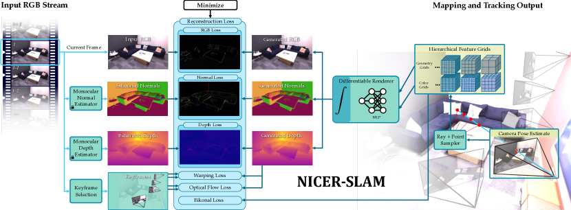
Figure 2: System Overview. Our method takes only an RGB stream as input and outputs both the camera poses as well as a learned hierarchical scene representation for geometry and colors. To realize an end-to-end joint mapping and tracking, we render predicted colors, depths, normals and optimize wrt. the input RGB and monocular cues. Moreover, we further enforce the geometric consistency with an RGB warping loss and an optical flow loss.

Dense Visual SLAM

SLAM is an active field in both industry and academia, especially in the past two decades. While sparse visual SLAM algorithms [32, 33, 13, 19] estimate accurate camera poses and only have sparse point clouds as the map representation, dense visual SLAM approaches focus on recovering a dense map of a scene. In general, map representations are categorized as either view-centric or world-centric. The first often represents 3D geometry as depth maps for keyframes, including the seminal work DTAM [35], as well as many follow-ups [58, 75, 56, 9, 55, 2, 74, 52, 57, 20]. Another line of research considers world-centric maps, and they anchor the 3D geometry of a full scene in uniform world coordinates and represent as surfels [63, 47] or occupancies/TSDF values in the voxel grids [3, 10, 37, 34]. Our work also falls into this category and uses a world-centric map representation, but instead of explicitly representing the surface, we store latent codes in multi-resolution voxel grids. This allows us to not only reconstruct high-quality geometry at low grid resolutions, but also attain plausible geometry estimation for unobserved regions.

Neural Implicit-based SLAM

Neural implicit representations [65] have shown great performance in many different tasks, including object-level reconstruction reconstruction [28, 4, 40, 41, 26, 36, 69], scene completion [42, 24, 17], novel view synthesis [29, 44, 72, 31, 64], etc. In terms of SLAM-related applications, some works [70, 23, 61, 6, 1, 8] try to jointly optimize a neural radiance field and camera poses, but they are only applicable to small objects or small camera movements. A series of recent works [7, 45] relax such constraints, but they mainly rely on state-of-the-art SLAM systems like ORB-SLAM and DROID-SLAM to obtain accurate camera poses, and do not produce 3D dense reconstruction but only novel view synthesis results.

iMAP [51] and NICE-SLAM [76] are the first two unified SLAM pipelines using neural implicit representations for both mapping and camera tracking. iMAP uses a single MLP as the scene representation so they are limited to small scenes, while NICE-SLAM can scale up to much larger indoor environments by applying hierarchical feature grids and tiny MLPs as the scene representation. Many follow-up works improve upon these two works from various perspectives, including efficient scene representation [18, 21], fast optimziation [67], add IMU measurements [25], or different shape representations [39, 30]. However, all of them require RGB-D inputs, which limits their applications in outdoor scenes or when only RGB sensors are available. In comparison, given only RGB sequences as input, our proposed neural-implicit-based system can output high-quality 3D reconstruction and recover accurate camera poses simultaneously.

A concurrent work [22] presents a system in a similar spirit to ours. While they optimize for accurate camera tracking, our method focuses on high-quality 3D reconstruction and novel view synthesis.

3 Method

We provide an overview of the NICER-SLAM pipeline in Fig. 2. Given an RGB video as input, we simultaneously estimate accurate 3D scene geometry and colors, as well as camera tracking via end-to-end optimization. We represent the scene geometry and appearance using hierarchical neural implicit representations (Sec. 3.1). With NeRF-like differentiable volume rendering, we can render color, depth, and normal values of every pixel (Sec. 3.2), which will be used for end-to-end joint optimization for camera pose, scene geometry, and color (Sec. 3.3). Finally we discuss some of the design choices made in our system (Sec. 3.4).

3.1 Hierarchical Neural Implicit Representations

We first introduce our optimizable hierarchical scene representations that combine multi-level grid features with MLP decoders for SDF and color predictions.

Coarse-level Geometric Representation

The goal of the coarse-level geometric representation is to efficiently model the coarse scene geometry (objects without capturing geometric details) and the scene layout (e.g. walls, floors) even with only partial observations. To this end, we represent the normalized scene with a dense voxel grid with a resolution of $32\times 32\times 32$, and keep a 32-dim feature in each voxel. For any point $\mathbf{x}\in\mathbb{R}^{3}$ in the space, we use a small MLP $f^{\text{coarse}}$ with a single 64-dim hidden layer to obtain its base SDF value $s^{\text{coarse}}\in\mathbb{R}$ and a geometric feature $\mathbf{z}^{\text{coarse}}\in\mathbb{R}^{32}$ as:

$${s^{\text{coarse}},\;\mathbf{z}^{\text{coarse}}}=f^{\text{coarse}}\big{(}\gamma(\mathbf{x}),\Phi^{\text{coarse}}(\mathbf{x})\big{)},$$ (1)

where $\gamma$ corresponds to a fixed positional encoding [29, 54] mapping the coordinate to higher dimension. Following [71, 69, 68], we set the level for positional encoding to 6. $\Phi^{\text{coarse}}(\mathbf{x})$ denotes that the feature grid $\Phi^{\text{coarse}}$ is tri-linearly interpolated at the point $\mathbf{x}$.

Fine-level Geometric Representation

While the coarse geometry can be obtained by our coarse-level shape representation, it is important to capture high-frequency geometric details in a scene. To realize it, we further model the high-frequency geometric details as residual SDF values with multi-resolution feature grids and an MLP decoder [5, 31, 76, 53]. Specifically, we employ multi-resolution dense feature grids $\{\Phi_{l}^{\text{fine}}\}^{L}_{1}$ with resolutions $R_{l}$. The resolutions are sampled in geometric space [31] to combine features at different frequencies:

$$R_{l}:=\;\lfloor R_{\text{min}}b^{l}\rfloor\hskip 8.5359ptb:=\;\text{exp}\left(\frac{\ln R_{\text{max}}-\ln R_{\text{min}}}{L-1}\right)\enspace,$$ (2)

where $R_{\text{min}},R_{\text{max}}$ correspond to the lowest and highest resolution, respectively. Here we consider $R_{\text{min}}=32$, $R_{\text{max}}=128$, and in total $L=8$ levels. The feature dimension is $4$ for each level.

Now, to model the residual SDF values for a point $\mathbf{x}$, we extract and concatenate the tri-linearly interpolated features at each level, and input them to an MLP $f^{\text{fine}}$ with 3 hidden layers of size 64:

$$(\,\Delta s,\;\mathbf{z}^{\text{fine}}\,)=f^{\text{fine}}\big{(}\gamma(\mathbf{x}),\;\{\Phi_{l}^{\text{fine}}(\mathbf{x})\}\big{)}\enspace,$$ (3)

where $\mathbf{z}^{\text{fine}}\in\mathbb{R}^{32}$ is the geometric feature for $\mathbf{x}$ at the fine level.

With the coarse-level base SDF value $s^{\text{coarse}}$ and the fine-level residual SDF $\Delta s$, the final predicted SDF value $\hat{s}$ for $\mathbf{x}$ is simply the sum between two:

$$\hat{s}=s^{\text{coarse}}+\Delta s\enspace.$$ (4)

Color Representation

Besides 3D geometry, we also predict color values such that our mapping and camera tracking can be optimized also with color losses. Moreover, as an additional application, we can also render images from novel views on the fly. Inspired by [31], we encode the color using another multi-resolution feature grid $\{\Phi_{l}^{\text{color}}\}_{1}^{L}$ and a decoder $f^{\text{color}}$ parameterized with a 2-layer MLP of size 64. The number of feature grid levels is now $L=16$, the features dimension is 2 at each level. The minimum and maximum resolution now become $R_{\text{min}}=16$ and $R_{\text{max}}=2048$, respectively. We predict per-point color values as:

$$\hat{\mathbf{c}}=f^{\text{color}}\big{(}\mathbf{x},\hat{\mathbf{n}},\gamma(\mathbf{v}),\mathbf{z}^{\text{coarse}},\mathbf{z}^{\text{fine}},\{\Phi_{l}^{\text{color}}(\mathbf{x})\}\big{)}\enspace.$$ (5)

where $\hat{\mathbf{n}}$ corresponds to the normal at point $\mathbf{x}$ calculated from $\hat{s}$ in Eq. (4), and $\gamma(\mathbf{v})$ is the viewing direction with positional encoding with a level of 4, following [68, 71].

3.2 Volume Rendering

Following recent works on implicit-based 3D reconstruction [38, 68, 71, 59] and dense visual SLAM [51, 76], we optimize our scene representation from Sec. 3.1 using differentiable volume rendering. More specifically, in order to render a pixel, we cast a ray $\mathbf{r}$ from the camera center $\mathbf{o}$ through the pixel along its normalized view direction $\mathbf{v}$. $N$ points are then sampled along the ray, denoted as $\mathbf{x}_{i}=\mathbf{o}+t_{i}\mathbf{v}$, and their predicted SDFs and color values are $\hat{s}_{i}$ and $\hat{\mathbf{c}}_{i}$, respectively. For volume rendering, we follow [68] to transform the SDFs $\hat{s}_{i}$ to density values $\sigma_{i}$:

$$\sigma_{\beta}(s)=\begin{cases}\frac{1}{2\beta}\exp\big{(}\frac{s}{\beta}\big{)}&\text{if }s\leq 0\\ \frac{1}{\beta}\left(1-\frac{1}{2}\exp\big{(}-\frac{s}{\beta}\big{)}\right)&\text{if }s>0\enspace,\end{cases}$$ (6)

where $\beta\in\mathbb{R}$ is a parameter controlling the transformation from SDF to volume density. As in [29], the color $\hat{C}$ for the current ray $\mathbf{r}$ is calculated as:

$$\begin{gathered}\hat{C}=\sum_{i=1}^{N}\,T_{i}\,\alpha_{i}\,\hat{\mathbf{c}}_{i}\hskip 14.22636ptT_{i}=\prod_{j=1}^{i-1}\left(1-\alpha_{j}\right)\\ \alpha_{i}=1-\exp\left(-\sigma_{i}\delta_{i}\right)\enspace,\end{gathered}$$ (7)

where $T_{i}$ and $\alpha_{i}$ correspond to transmittance and alpha value of sample point $i$ along ray $\mathbf{r}$, respectively, and $\delta_{i}$ is the distance between neighboring sample points. In a similar manner, we can also compute the depth $\hat{D}$ and normal $\hat{N}$ of the surface intersecting the current ray $\mathbf{r}$ as:

$$\hat{D}=\sum_{i=1}^{N}\,T_{i}\,\alpha_{i}\,t_{i}\hskip 28.45274pt\hat{N}=\sum_{i=1}^{N}\,T_{i}\,\alpha_{i}\,\hat{\mathbf{n}}_{i}\enspace.$$ (8)

Locally Adaptive Transformation

The $\beta$ parameter in Eq. (6) models the smoothing amount near the object’s surface. The value of $\beta$ gradually decreases during the optimization process as the network becomes more certain about the object surface. Therefore, this optimization scheme results in faster and sharper reconstructions.

In VolSDF [68], they model $\beta$ as a single global parameter. This way of modeling the transformation intrinsically assumes that the degree of optimization is the same across different regions of the scene, which is sufficient for small object-level scenes. However, for our sequential input setting within a complicated indoor scene, a global optimizable $\beta$ is sub-optimal (cf. ablation study in Sec. 4.2). Therefore, we propose to assign $\beta$ values locally so the SDF-density transformation in Eq. (6) is also locally adaptive.

In detail, we maintain a voxel counter across the scene and count the number of point samples within every voxel during the mapping process. We empirically choose the voxel size of $64^{3}$ (see ablation study in Sec. 4.2). Next, we heuristically design a transformation from local point samples counts $T_{p}$ to the $\beta$ value:

$$\beta=c_{0}\cdot\exp(-c_{1}\cdot T_{p})+c_{2}\enspace.$$ (9)

We come up with the transformation by plotting $\beta$ decreasing curve with respect to the voxel count under the global input setting, and fitting a function on the curve. We empirically find that the exponential curve is the best fit.

3.3 End-to-End Joint Mapping and Tracking

Purely from an RGB sequential input, it is very difficult to jointly optimize 3D scene geometry and color together with camera poses, due to the high degree of ambiguity, especially for large complex scenes with many textureless and sparsely covered regions. Therefore, to enable end-to-end joint mapping and tracking under our neural scene representation, we propose to use the following loss functions, including geometric and prior constraints, single- and multi-view constraints, as well as both global and local constraints.

RGB Rendering Loss

Eq. (7) connects the 3D neural scene representation to 2D observations, hence, we can optimize the scene representation with a simple RGB reconstruction loss:

$$\mathcal{L}_{\text{rgb}}=\sum_{\mathbf{r}\in\mathcal{R}}{\lVert\hat{C}(\mathbf{r})-C(\mathbf{r})\rVert}_{1}\enspace,$$ (10)

where $\mathcal{R}$ denotes the randomly sampled pixels/rays in every iteration, and $C$ is the input pixel color value.

RGB Warping Loss

To further enforce geometry consistency from only color inputs, we also add a simple per-pixel warping loss.

For a pixel in frame $m$, denoted as $\mathbf{r}_{m}$, we first render its depth value using Eq. (8) and unproject it to 3D, and then project it to another frame $n$ using intrinsic and extrinsic parameters of frame $n$. The projected pixel $\mathbf{r}_{m\rightarrow n}$ in the nearby keyframe $n$ is denoted as $\mathbf{r}_{m\rightarrow n}$. The warping loss is then defined as:

$$\mathcal{L}_{\text{warp}}=\sum_{\mathbf{r}_{m}\in\mathcal{R}}\sum_{n\in\mathcal{K}_{m}}{\lVert C(\mathbf{r}_{m})-C(\mathbf{r}_{m\rightarrow n})\rVert}_{1}\enspace,$$ (11)

where $\mathcal{K}_{m}$ denotes the keyframe list for the current frame $m$, excluding frame $m$ itself. We mask out the pixels that are projected outside the image boundary of frame $n$. Note that unlike [11] that optimize neural implicit surfaces with patch warping, we observed that it is way more efficient and without performance drop to simply perform warping on randomly sampled pixels.

Optical Flow Loss

Both the RGB rendering and the warping loss are only point-wise terms which are prone to local minima. We therefore add a loss that is based on optical flow estimates which adhere to regional smoothness priors and help to tackle ambiguities. Suppose the sample pixel in frame $m$ as $\mathbf{r}_{m}$ and the corresponding projected pixel in frame $n$ as $\mathbf{r}_{n}$, we can add an optical flow loss as follows:

$$\mathcal{L}_{\text{flow}}=\sum_{\mathbf{r}_{m}\in\mathcal{R}}\sum_{n\in\mathcal{K}_{m}}{\lVert(\mathbf{r}_{m}-\mathbf{r}_{n})-\text{GM}(\mathbf{r}_{m\rightarrow n})\rVert}_{1}\enspace,$$ (12)

where $\text{GM}(\mathbf{r}_{m\rightarrow n})$ denotes the estimated optical flow from GMFlow [66].

Monocular Depth Loss

Given RGB input, one can easily obtain geometric cues (such as depths or normals) via an off-the-shelf monocular predictor [12]. Inspired by [71], we also include this information into the optimization to guide the neural implicit surface reconstruction.

More specifically, to enforce depth consistency between our rendered expected depths $\hat{D}$ and the monocular depths $\bar{D}$, we use the following loss [43, 71]:

$$\mathcal{L}_{\text{depth}}=\sum_{\mathbf{r}\in\mathcal{R}}{\lVert(w\hat{D}(\mathbf{r})+q)-\bar{D}(\mathbf{r})\rVert}^{2}\enspace,$$ (13)

where $w,q\in\mathbb{R}$ are the scale and shift used to align $\hat{D}$ and $\bar{D}$, since $\bar{D}$ is only known up to an unknown scale. We solve for $w$ and $q$ per image with a least-squares criterion [43], which has a closed-form solution.

Monocular Normal Loss

Another geometric cue that is complementary to the monocular depth is surface normal. Unlike monocular depths that provide global surface information for the current view, surface normals are local and capture more geometric details. Similar to [71], we impose consistency on the volume-rendered normal $\hat{N}$ and the monocular normals $\bar{N}$ from [12] with angular and L1 losses:

$$\mathcal{L}_{\text{normal}}=\sum_{\mathbf{r}\in\mathcal{R}} {\lVert\hat{N}(\mathbf{r})-\bar{N}(\mathbf{r})\rVert}_{1}$$ (14)

$$+ {\lVert 1-\hat{N}(\mathbf{r})^{\top}\bar{N}(\mathbf{r})\rVert}_{1}\enspace.$$

Eikonal Loss

In addition, we add the Eikonal loss [15] to regularize the output SDF values $\hat{s}$:

$$\mathcal{L}_{\text{eikonal}}=\sum_{\mathbf{x}\in\mathcal{X}}({\lVert\nabla\hat{s}(\mathbf{x})\rVert}_{2}-1)^{2}\enspace,$$ (15)

where $\mathcal{X}$ are a set of uniformly sampled near-surface points.

Optimization Scheme

Finally, we provide details on how to optimize the scene geometry and appearance in the form of our hierarchical representation, and also the camera poses.

Mapping: To optimize the scene representation mentioned in Sec. 3.1, we uniformly sample $M$ pixels/rays in total from the current frame and selected keyframes. Next, we perform a 3-stage optimization similar to [76] but use the following loss:

$$\begin{split}\mathcal{L}\!=\!\mathcal{L}_{\text{rgb}}&+0.5\mathcal{L}_{\text{warp}}+0.001\mathcal{L}_{\text{flow}}\\ &+0.1\mathcal{L}_{\text{depth}}+0.05\mathcal{L}_{\text{normal}}+0.1\mathcal{L}_{\text{eikonal}}\end{split}$$ (16)

At the first stage, we treat the coarse-level base SDF value $s^{\text{coarse}}$ in Eq. (1) as the final SDF value $\hat{s}$, and optimize the coarse feature grid $\Phi^{\text{coarse}}$, coarse MLP parameters of $f^{\text{coarse}}$, and color MLP parameters of $f^{\text{color}}$ with Eq. (16). Next, after $25\%$ of the total number of iterations, we start using Eq. (4) as the final SDF value so the fine-level feature grids $\{\Phi_{l}^{\text{fine}}\}$ and fine-level MLP $f^{\text{fine}}$ are also jointly optimized. Finally, after $75\%$ of the total number of iterations, we conduct a local bundle adjustment (BA) with Eq. (16), where we also include the optimization of color feature grids $\{\Phi_{l}^{\text{color}}\}$ as well as the extrinsic parameters of $K$ selected mapping frames.

Camera Tracking: We run in parallel camera tracking to optimize the camera pose (rotation and translation) of the current frame, while keeping the hierarchical scene representation fixed. Straightforwardly, we sample $M_{t}$ pixels from the current frame and use purely the RGB rendering loss in Eq. (10) for 100 iterations.

3.4 System Design

Frame Selection for Mapping

During the mapping process, we need to select multiple frames from which we sample rays and pixels. We introduce a simple frame selection mechanism. First, we maintain a global keyframe list for which we directly add one every 10 frames. For mapping, we select in total $K=16$ frames, where 5 of them are randomly selected from the keyframe list, 10 are randomly selected from the latest 20 keyframes, and also the current frame.

Implementation Details

Mapping is done every 5 frames, while tracking is done every frame. Note that with the pure RGB input, drifting is a known hard problem. To alleviate this, during the local BA stage in mapping, we freeze the camera poses for half of the 16 selected frames which are far from the current frame, and only optimize the camera poses of the other half jointly with the scene representation. For the adaptive local transformation in Eq. (9), we set $c_{0}=1.208\cdot 10^{-2}$, $c_{1}=6.26471\cdot 10^{-6}$ and $c_{2}=2.3\cdot 10^{-3}$. For mapping and tracking, we sample $M=8096$ and $M_{t}=1024$ pixels, respectively, and optimize for 100 iterations. For every mapping iteration, we randomly sample pixels from all selected frames, instead of one frame per iteration. With our current unoptimized PyTorch implementation, it takes on average 496ms and 147ms for each mapping and tracking iteration on a single A100 GPU. The coarse geometry is initialized as a sphere following [71, 68, 69]. To optimize the scene representation during the first mapping step, we assign the scale and shift value as $w=20$ and $q=0$ in Eq. (13), so that the scaled monocular depth values are roughly reasonable (e.g. 1-5 meters). The final mesh is extracted from the scene representation using Marching Cubes [27] with a resolution of $512^{3}$.

4 Experiments

We evaluate qualitative and quantitative comparisons against state-of-the-art (SOTA) SLAM frameworks on both synthetic and real-world datasets in Sec. 4.1. A comprehensive ablation study that supports our design choices is also provided in Sec. 4.2.

Datasets

We first evaluate on a synthetic dataset Replica [49], where RGB-(D) images can be rendered out with the official renderer. To verify the robustness of our approach, we compare a challenging real-world dataset 7-Scenes [48]. It consists of low-resolution images with severe motion blurs. We use COLMAP to obtain the intrinsic parameters of the RGB camera.

Baselines

We compare to (a) SOTA neural implicit-based RGB-D SLAM system NICE-SLAM [76] and Vox-Fusion [67], (b) classic MVS method COLMAP [46], and (c) SOTA dense monocular SLAM system DROID-SLAM [57]. For camera tracking evaluation, we also compare to DROID-SLAM^∗, which does not perform the final global bundle adjustment and loop closure (identical to our NICER-SLAM setting). For DROID-SLAM’s 3D reconstruction, we run TSDF fusion with their predicted depths of keyframes.

Metrics

For camera tracking, we follow the conventional monocular SLAM evaluation pipeline where the estimated trajectory is aligned to the GT trajectory using evo [16], and then evaluate the accuracy of camera tracking (ATE RMSE) [50]. To evaluate scene geometry, we consider Accuracy, Completion, Completion Ratio, and Normal Consistency. The reconstructed meshes from monocular SLAM systems are aligned to the GT mesh using the ICP tool from [14]. Moreover, we use PSNR, SSIM [60] and LPIPS [73] for novel view synthesis evaluation.

		rm-0	rm-1	rm-2	off-0	off-1	off-2	off-3	off-4	Avg.
RGB-D input
NICE-SLAM	Acc.[cm]$\downarrow$	3.53	3.60	3.03	5.56	3.35	4.71	3.84	3.35	3.87
	Comp.[cm]$\downarrow$	3.40	3.62	3.27	4.55	4.03	3.94	3.99	4.15	3.87
	Comp.Ratio[$<\!5$cm %]$\uparrow$	86.05	80.75	87.23	79.34	82.13	80.35	80.55	82.88	82.41
	Normal Cons.[%]$\uparrow$	91.92	91.36	90.79	89.30	88.79	88.97	87.18	91.17	89.93
Vox-Fusion	Acc.[cm]$\downarrow$	2.53	1.69	3.33	2.20	2.21	2.72	4.16	2.48	2.67
	Comp.[cm]$\downarrow$	2.81	2.51	4.03	8.75	7.36	4.19	3.26	3.49	4.55
	Comp.Ratio[$<\!5$cm %]$\uparrow$	91.52	91.34	86.78	81.99	82.03	85.45	87.13	86.53	86.59
	Normal Cons.[%]$\uparrow$	94.14	93.28	91.71	90.52	88.95	91.54	91.03	92.67	91.73
RGB input
COLMAP	Acc.[cm]$\downarrow$	3.87	27.29	5.41	5.21	12.69	4.28	5.29	5.45	8.69
	Comp.[cm]$\downarrow$	4.78	23.90	17.42	12.98	12.35	4.96	16.17	4.41	12.12
	Comp.Ratio[$<\!5$cm %]$\uparrow$	83.08	22.89	64.47	72.59	69.52	81.12	64.38	82.92	67.62
	Normal Cons.[%]$\uparrow$	72.49	60.10	69.42	69.91	74.04	71.84	71.49	71.75	70.13
DROID-SLAM	Acc.[cm]$\downarrow$	12.18	8.35	3.26	3.01	2.39	5.66	4.49	4.65	5.50
	Comp.[cm]$\downarrow$	8.96	6.07	16.01	16.19	16.20	15.56	9.73	9.63	12.29
	Comp.Ratio[$<\!5$cm %]$\uparrow$	60.07	76.20	61.62	64.19	60.63	56.78	61.95	67.51	63.62
	Normal Cons.[%]$\uparrow$	72.81	74.71	79.21	77.53	78.57	75.79	77.69	76.38	76.59
NICER-SLAM	Acc.[cm]$\downarrow$	2.53	3.93	3.40	5.49	3.45	4.02	3.34	3.03	3.65
	Comp.[cm]$\downarrow$	3.04	4.10	3.42	6.09	4.42	4.29	4.03	3.87	4.16
	Comp.Ratio[$<\!5$cm %]$\uparrow$	88.75	76.61	86.10	65.19	77.84	74.51	82.01	83.98	79.37
	Normal Cons.[%]$\uparrow$	93.00	91.52	92.38	87.11	86.79	90.19	90.10	90.96	90.27

Table 1: Reconstruction Results on the Replica dataset. Best results are highlighted as first, second, and third. NICER-SLAM performs the best among RGB SLAM methods, and is also on par with RGB-D methods.

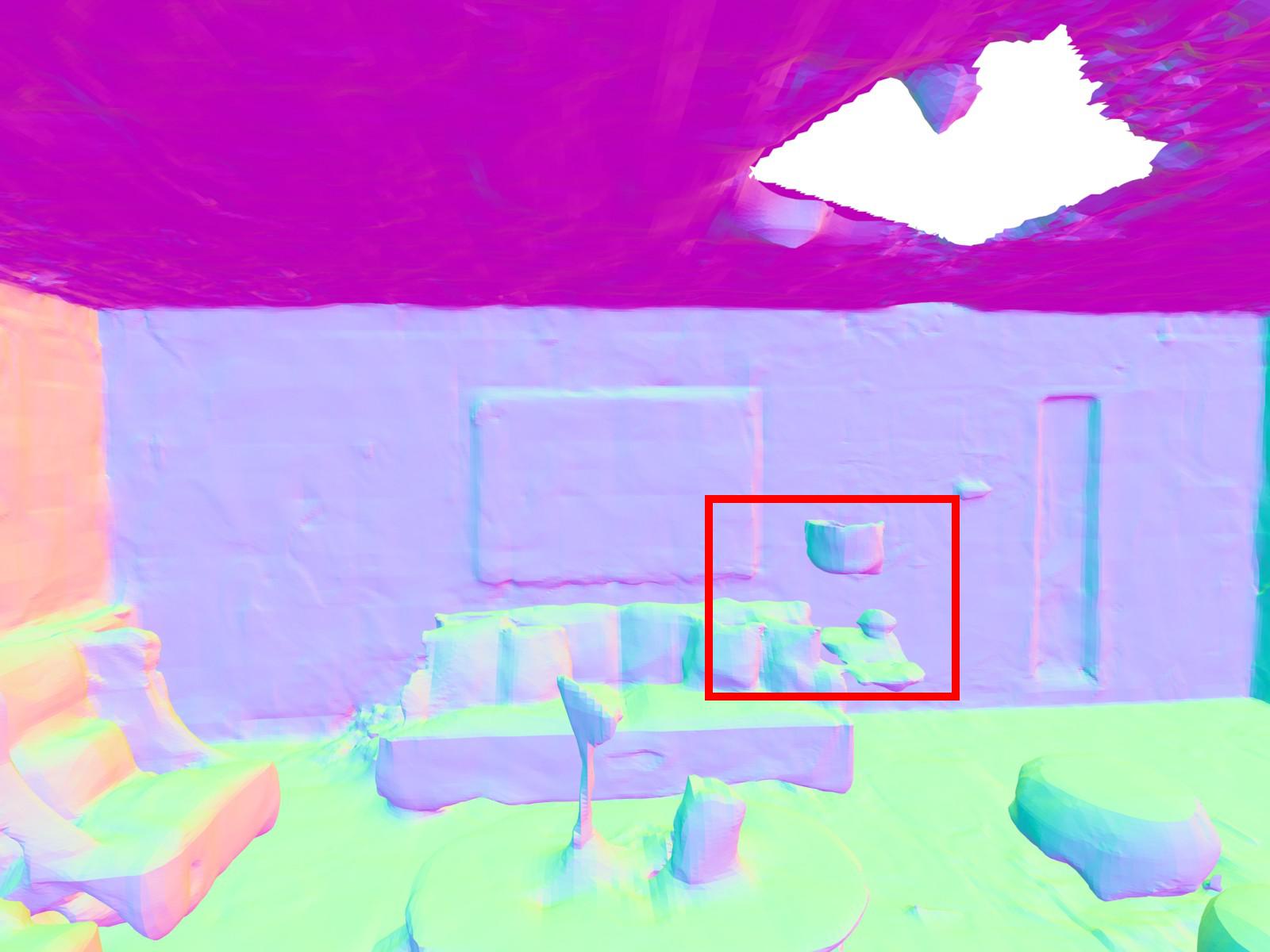
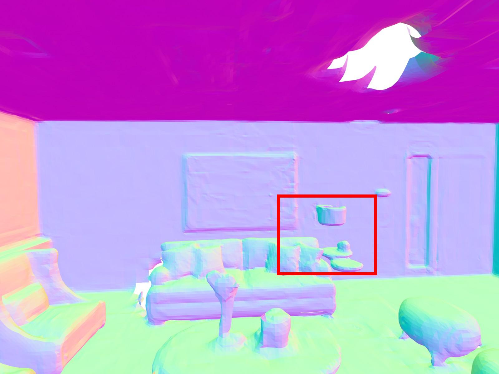
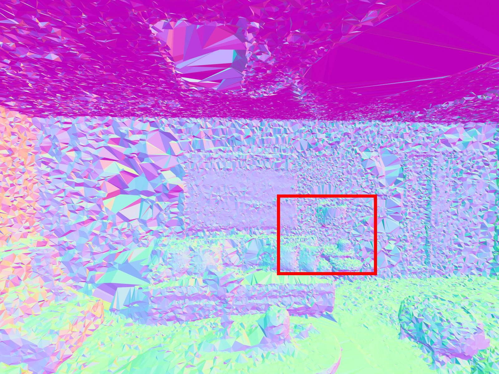
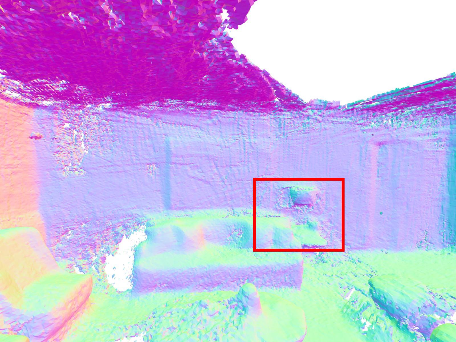
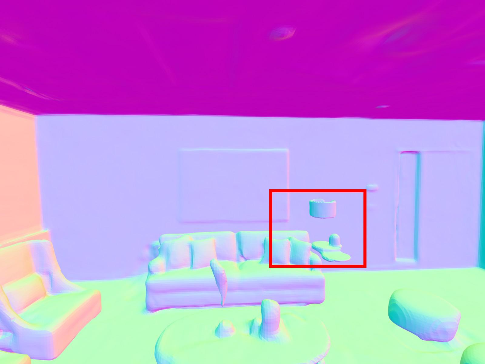
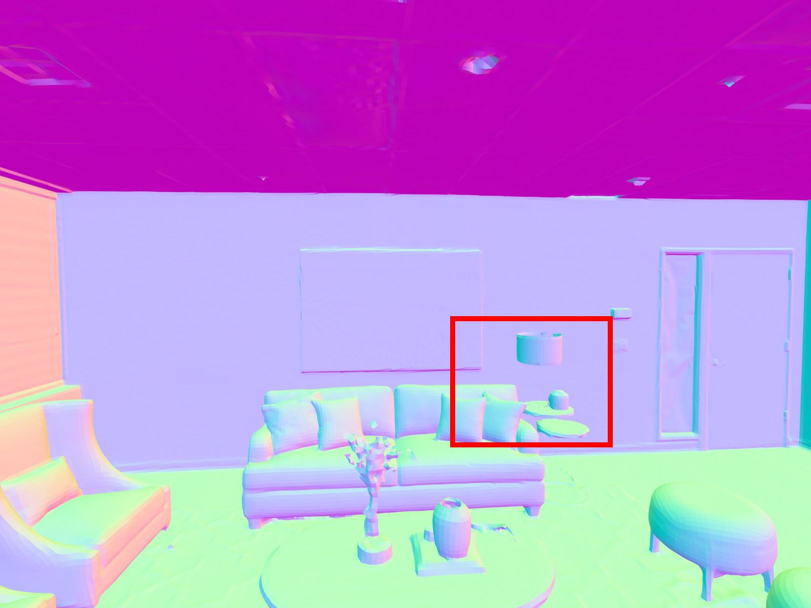
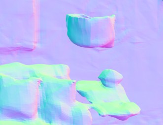
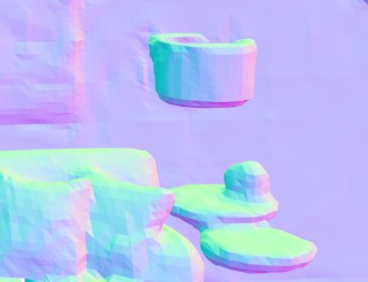
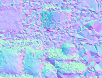
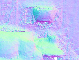
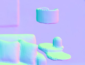
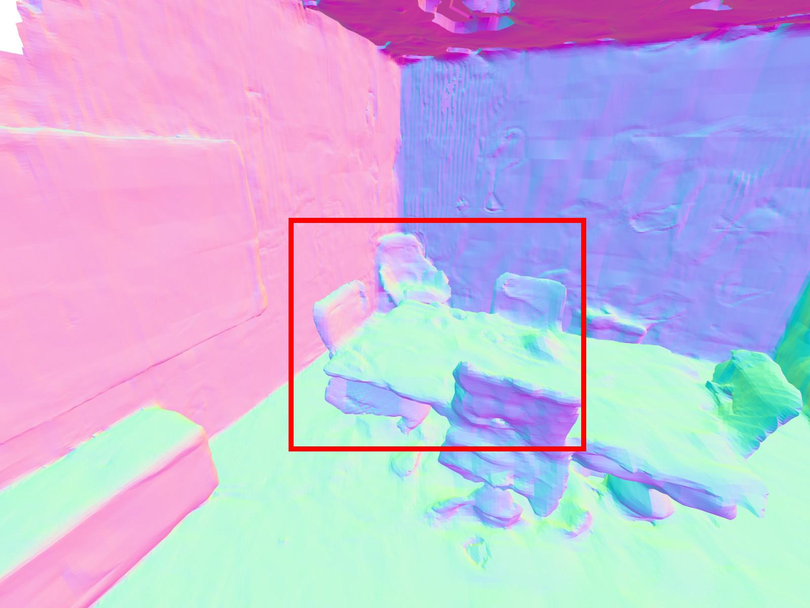
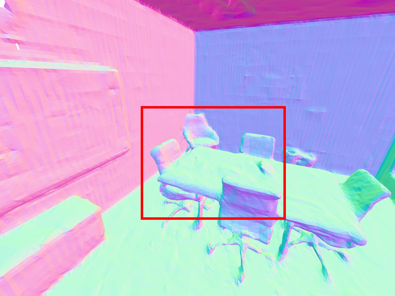
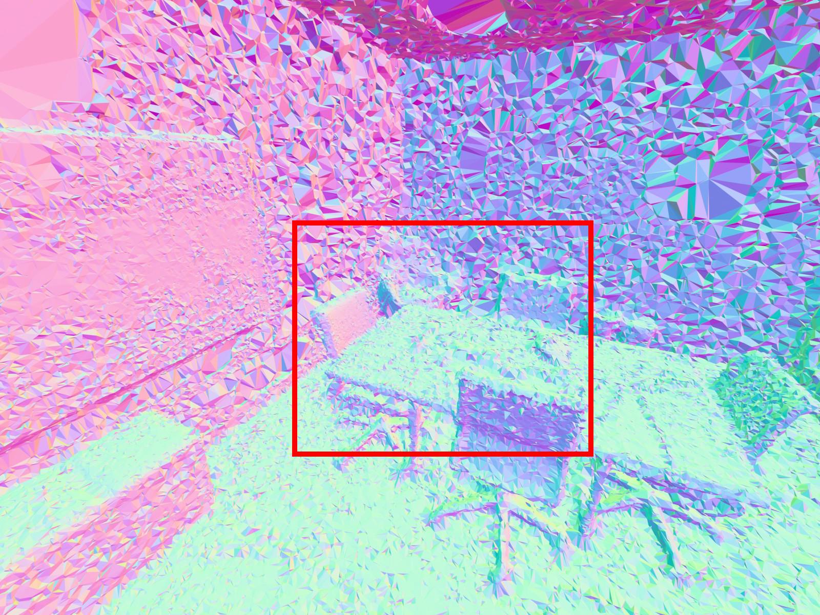
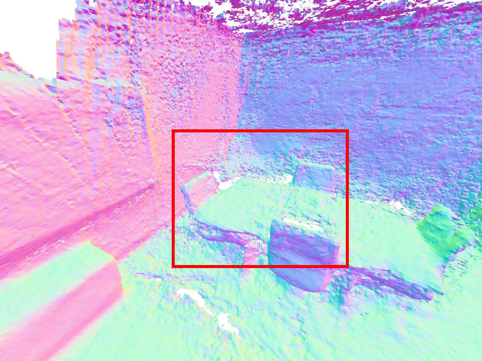
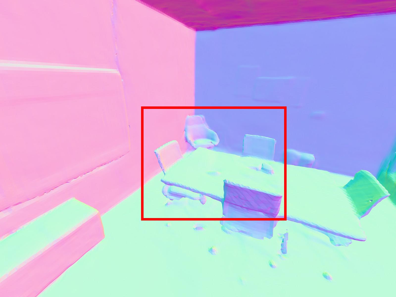
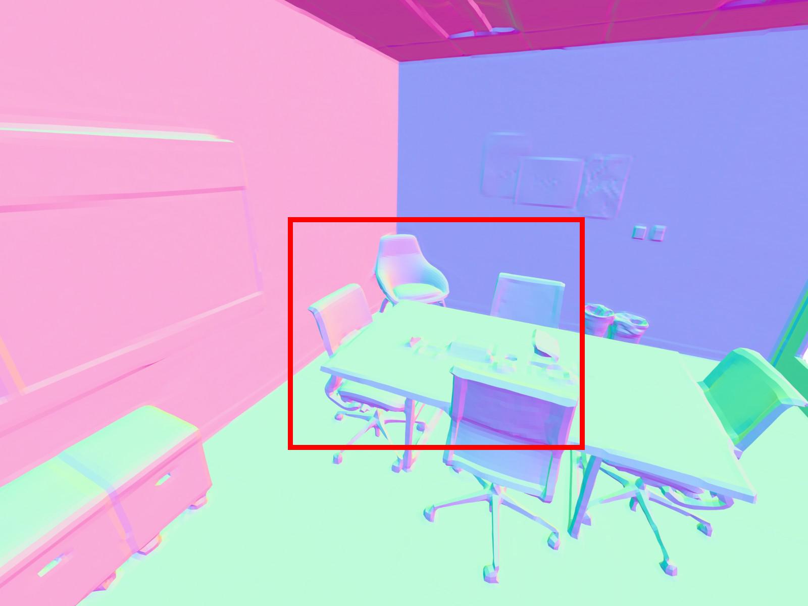
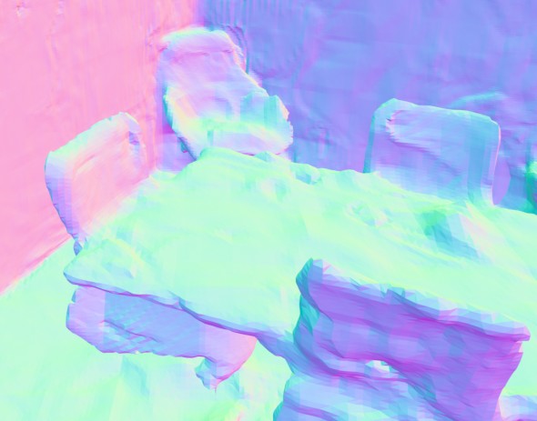
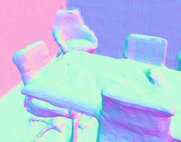
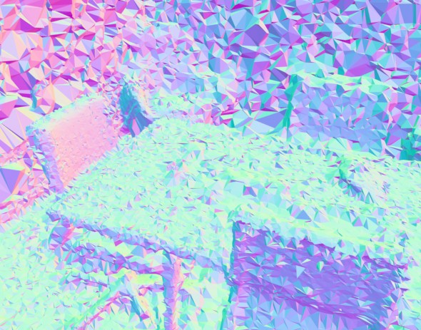
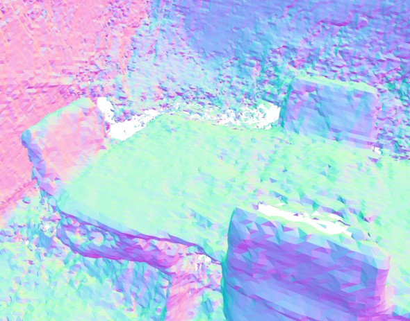
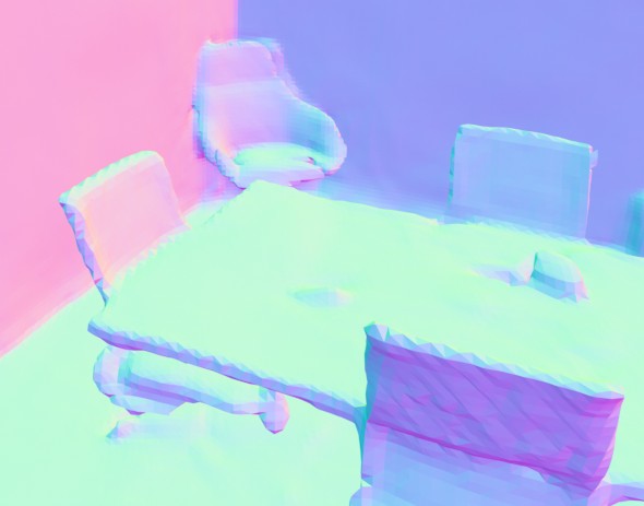
NICE-SLAM	Vox-Fusion	COLMAP	DROID-SLAM	NICER-SLAM	GT
RGB-D input		RGB input

Figure 3: 3D Reconstruction Results on the Replica Dataset [49]. The second and fourth row show zoom-in normal maps.

	rm-0	rm-1	rm-2	off-0	off-1	off-2	off-3	off-4	Avg.
RGB-D input
NICE-SLAM	1.69	2.04	1.55	0.99	0.90	1.39	3.97	3.08	1.95
Vox-Fusion	0.27	1.33	0.47	0.70	1.11	0.46	0.26	0.58	0.65
RGB input
COLMAP	0.62	23.7	0.39	0.33	0.24	0.79	0.14	1.73	3.49
DROID-SLAM	0.34	0.13	0.27	0.25	0.42	0.32	0.52	0.40	0.33
DROID-SLAM∗	0.58	0.58	0.38	1.06	0.40	0.70	0.53	1.33	0.70
NICER-SLAM	1.36	1.60	1.14	2.12	3.23	2.12	1.42	2.01	1.88

Table 2: Camera Tracking Results on the Replica Dataset [49]. ATE RMSE [cm] ($\downarrow$) is used as the evaluation metric.

			rm-0	rm-1	rm-2	off-0	off-1	off-2	off-3	off-4	Avg.
RGB-D input
NICE-SLAM	Extra- polate	PSNR $\uparrow$	23.83	22.61	21.97	25.78	25.30	18.50	22.82	25.26	23.26
		SSIM $\uparrow$	0.788	0.813	0.858	0.887	0.842	0.826	0.862	0.875	0.844
		LPIPS $\downarrow$	0.284	0.249	0.218	0.209	0.145	0.242	0.190	0.191	0.216
2-12	Inter- polate	PSNR $\uparrow$	22.12	22.47	24.52	29.07	30.34	19.66	22.23	24.94	24.42
		SSIM $\uparrow$	0.689	0.757	0.814	0.874	0.886	0.797	0.801	0.856	0.809
		LPIPS $\downarrow$	0.330	0.271	0.208	0.229	0.181	0.235	0.209	0.198	0.233
Vox-Fusion	Extra- polate	PSNR $\uparrow$	23.45	20.83	18.38	23.28	24.48	17.50	23.06	24.84	21.98
		SSIM $\uparrow$	0.765	0.773	0.747	0.751	0.762	0.727	0.824	0.851	0.775
		LPIPS $\downarrow$	0.280	0.272	0.282	0.235	0.169	0.292	0.232	0.212	0.247
2-12	Inter- polate	PSNR $\uparrow$	22.39	22.36	23.92	27.79	29.83	20.33	23.47	25.21	24.41
		SSIM $\uparrow$	0.683	0.751	0.798	0.857	0.876	0.794	0.803	0.847	0.801
		LPIPS $\downarrow$	0.303	0.269	0.234	0.241	0.184	0.243	0.213	0.199	0.236
RGB input
COLMAP	Extra- polate	PSNR $\uparrow$	20.93	11.67	10.35	5.88	5.88	15.66	13.73	17.47	12.70
		SSIM $\uparrow$	0.778	0.698	0.757	0.595	0.539	0.806	0.792	0.811	0.722
		LPIPS $\downarrow$	0.291	0.443	0.330	0.444	0.337	0.303	0.299	0.273	0.340
2-12	Inter- polate	PSNR $\uparrow$	20.31	12.33	14.53	9.39	7.26	15.42	15.28	16.98	13.94
		SSIM $\uparrow$	0.710	0.607	0.771	0.744	0.676	0.767	0.754	0.765	0.724
		LPIPS $\downarrow$	0.332	0.531	0.318	0.377	0.306	0.341	0.330	0.290	0.353
DROID-SLAM	Extra- polate	PSNR $\uparrow$	18.25	18.65	13.49	16.13	10.31	14.78	15.53	15.71	15.36
		SSIM $\uparrow$	0.737	0.793	0.786	0.760	0.650	0.800	0.797	0.800	0.765
		LPIPS $\downarrow$	0.352	0.283	0.299	0.298	0.286	0.300	0.302	0.311	0.304
2-12	Inter- polate	PSNR $\uparrow$	21.41	24.04	22.08	23.59	21.29	20.64	20.22	20.22	21.69
		SSIM $\uparrow$	0.693	0.786	0.826	0.868	0.863	0.828	0.808	0.819	0.812
		LPIPS $\downarrow$	0.329	0.270	0.228	0.232	0.207	0.231	0.234	0.237	0.246
NICER-SLAM	Extra- polate	PSNR $\uparrow$	25.64	23.69	22.62	25.88	22.56	21.46	24.42	25.15	23.93
		SSIM $\uparrow$	0.810	0.820	0.871	0.885	0.828	0.863	0.888	0.887	0.857
		LPIPS $\downarrow$	0.254	0.233	0.200	0.193	0.160	0.203	0.175	0.192	0.201
2-12	Inter- polate	PSNR $\uparrow$	25.33	23.92	26.12	28.54	25.86	21.95	26.13	25.47	25.41
		SSIM $\uparrow$	0.751	0.771	0.831	0.866	0.852	0.820	0.856	0.865	0.827
		LPIPS $\downarrow$	0.250	0.215	0.176	0.172	0.178	0.195	0.162	0.177	0.191

Table 3: Novel View Synthesis Evaluation on Replica dataset [49]. Best results are highlighted as first, second, and third. Our method mostly outperforms all other methods even the ones that additionally use depth inputs.

4.1 Mapping, Tracking and Rendering Evaluations

Evaluation on Replica [49]

First of all, for the evaluation of scene geometry, as shown in Table 1, our method significantly outperforms RGB-only baselines like DROID-SLAM and COLMAP, and even shows competitive performance against RGB-D SLAM approaches like NICE-SLAM and Vox-Fusion. Moreover, due to the use of monocular depth and normal cues, we show in Fig. 3 that our reconstructions can faithfully recover geometric details and attain the most visually appealing results among all methods. For camera tracking, we can clearly see on Table 2 that the state-of-the-art method DROID-SLAM outperforms all methods including those RGB-D SLAM systems. Nevertheless, our method is still on par with NICE-SLAM (1.88 vs 1.95 cm on average), while no ground truth depths are used as additional input.

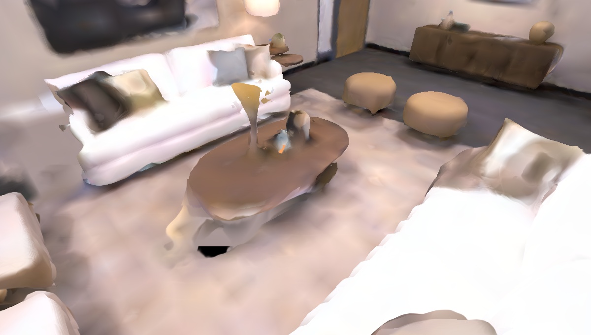
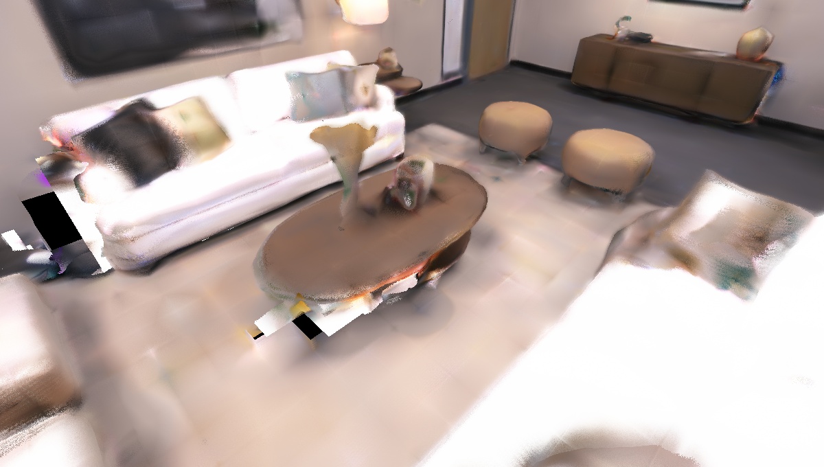
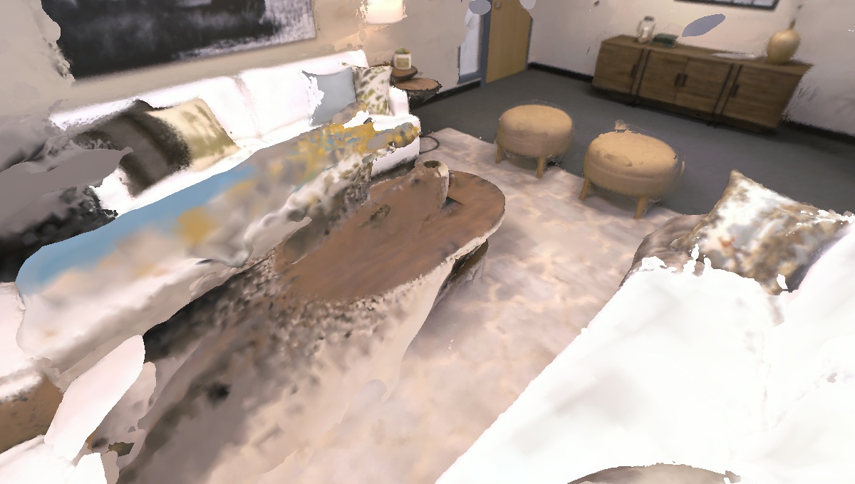
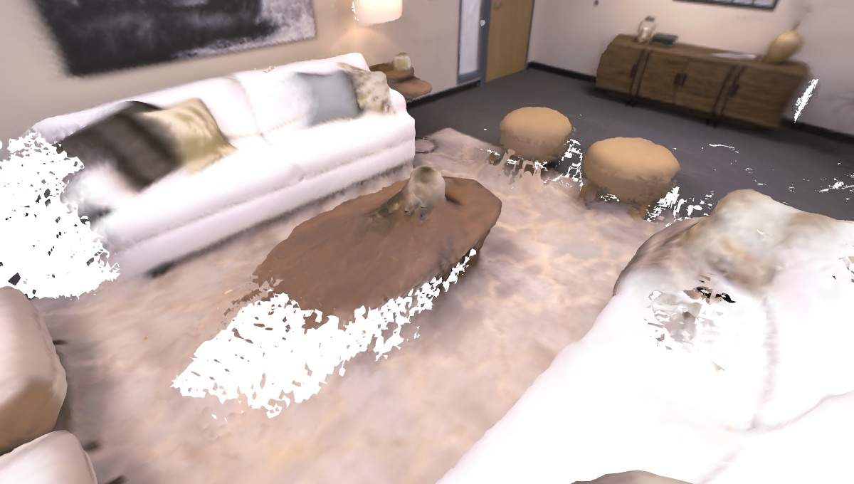
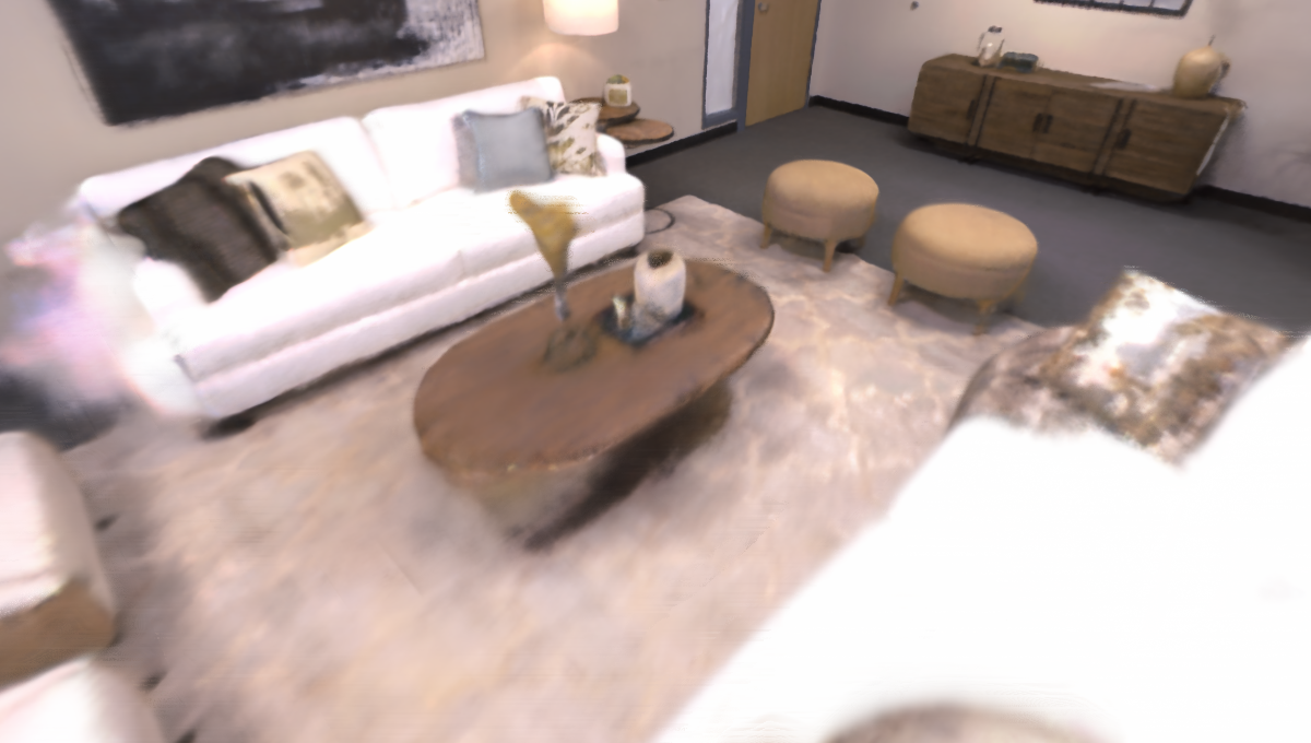
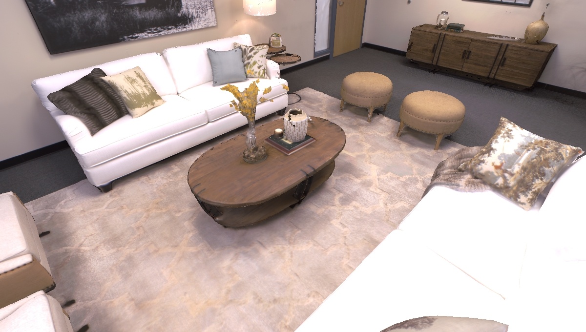
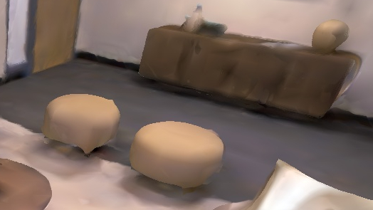
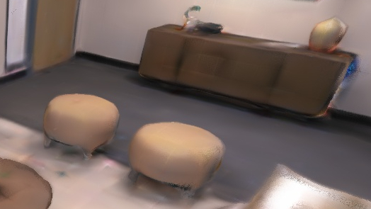
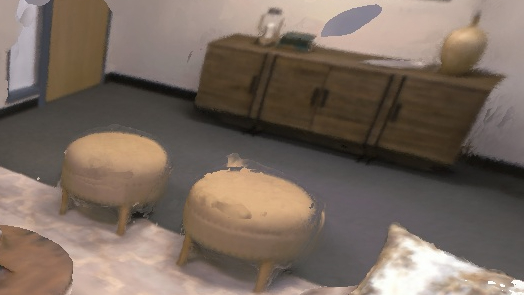
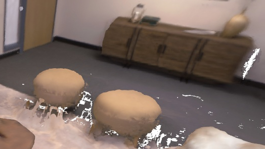
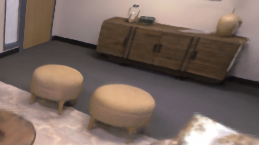
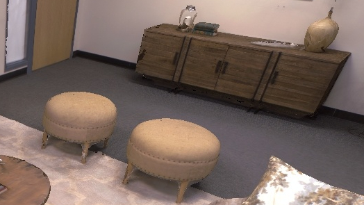
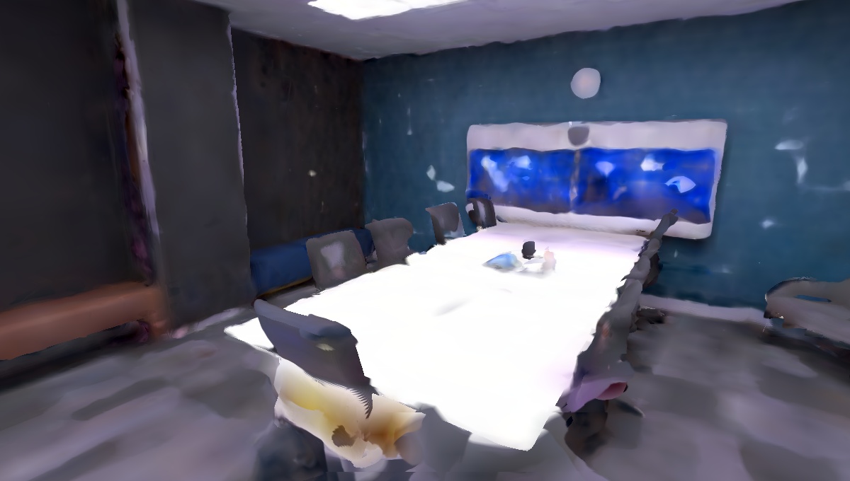
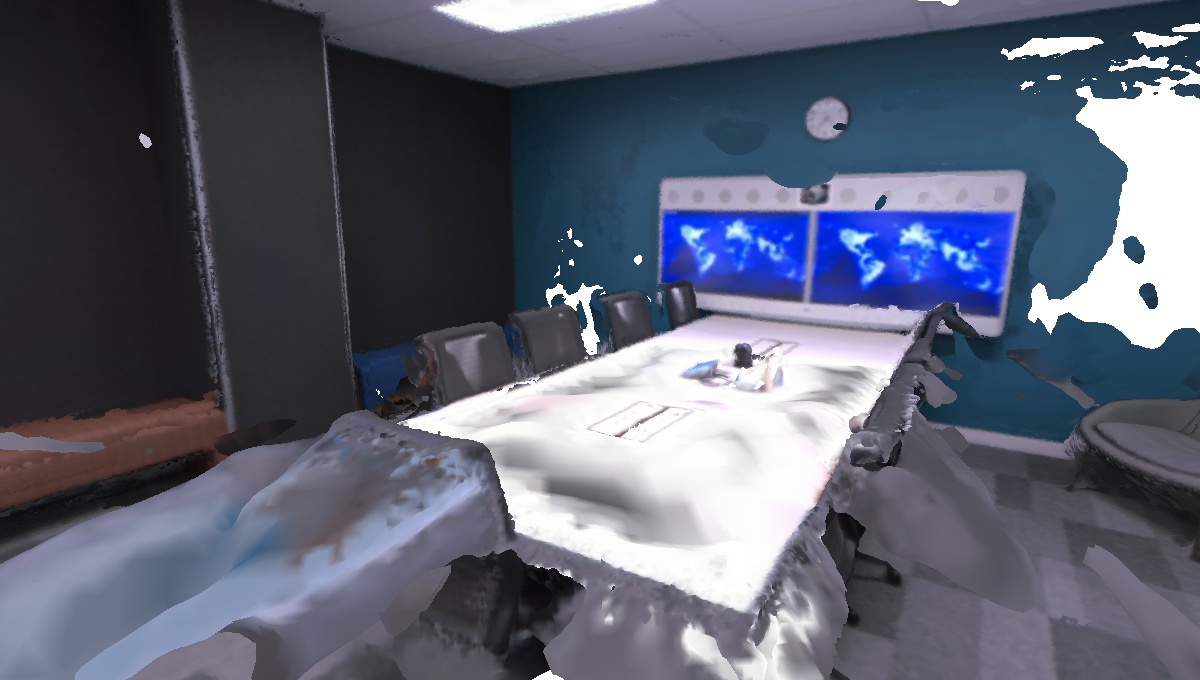
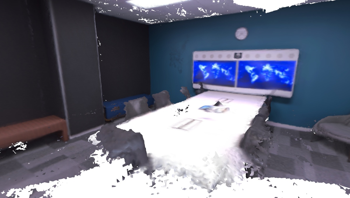
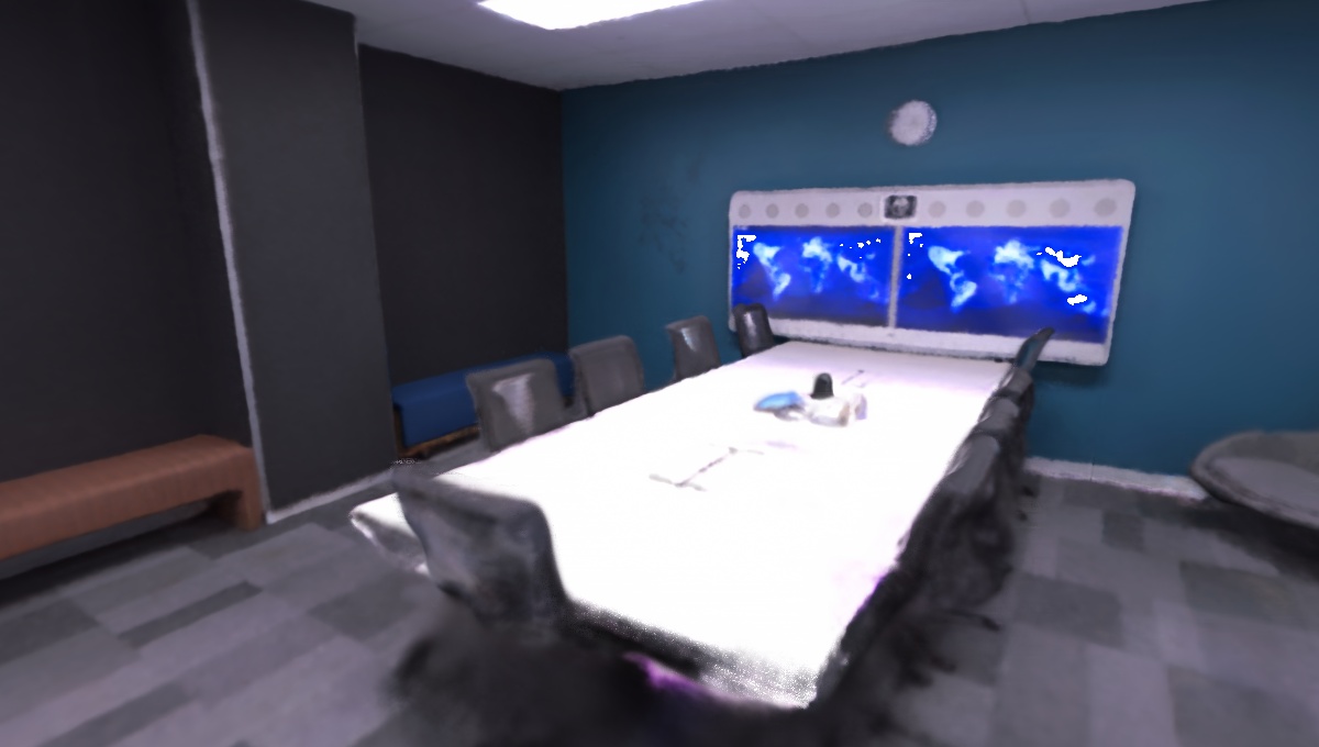
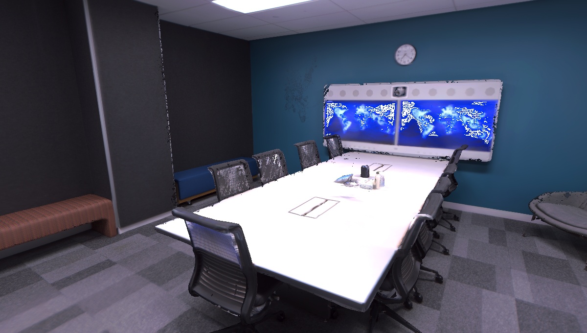
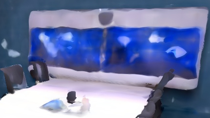
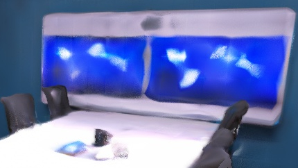
NICE-SLAM	Vox-Fusion	COLMAP	DROID-SLAM	NICER-SLAM	GT
RGB-D input		RGB input

Figure 4: Novel View Synthesis Results on the Replica the Dataset [49]. The second and fourth row show zoom-in renderings for better comparison. Note that we selected novel viewpoints far from the input views (extrapolation).

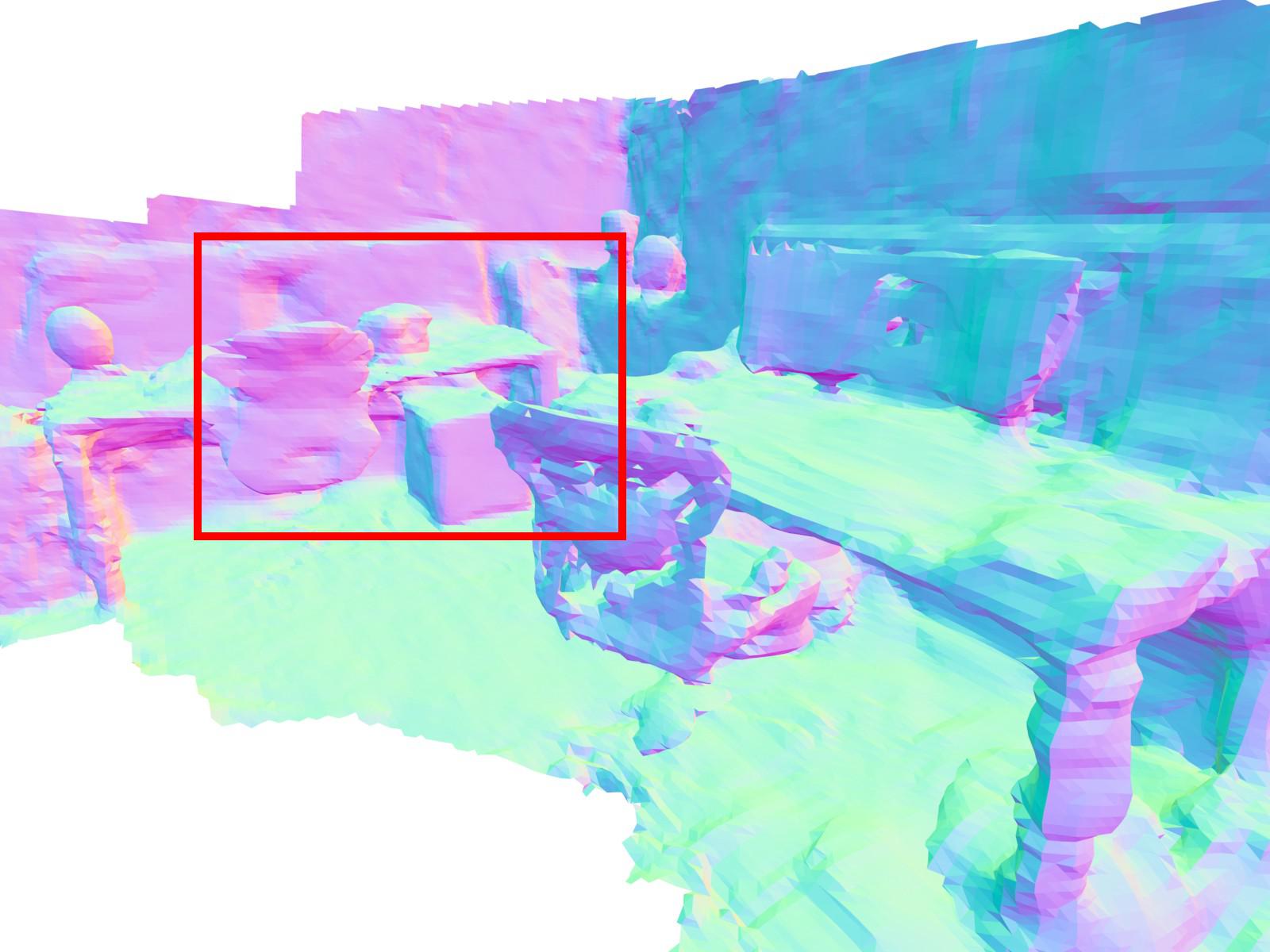
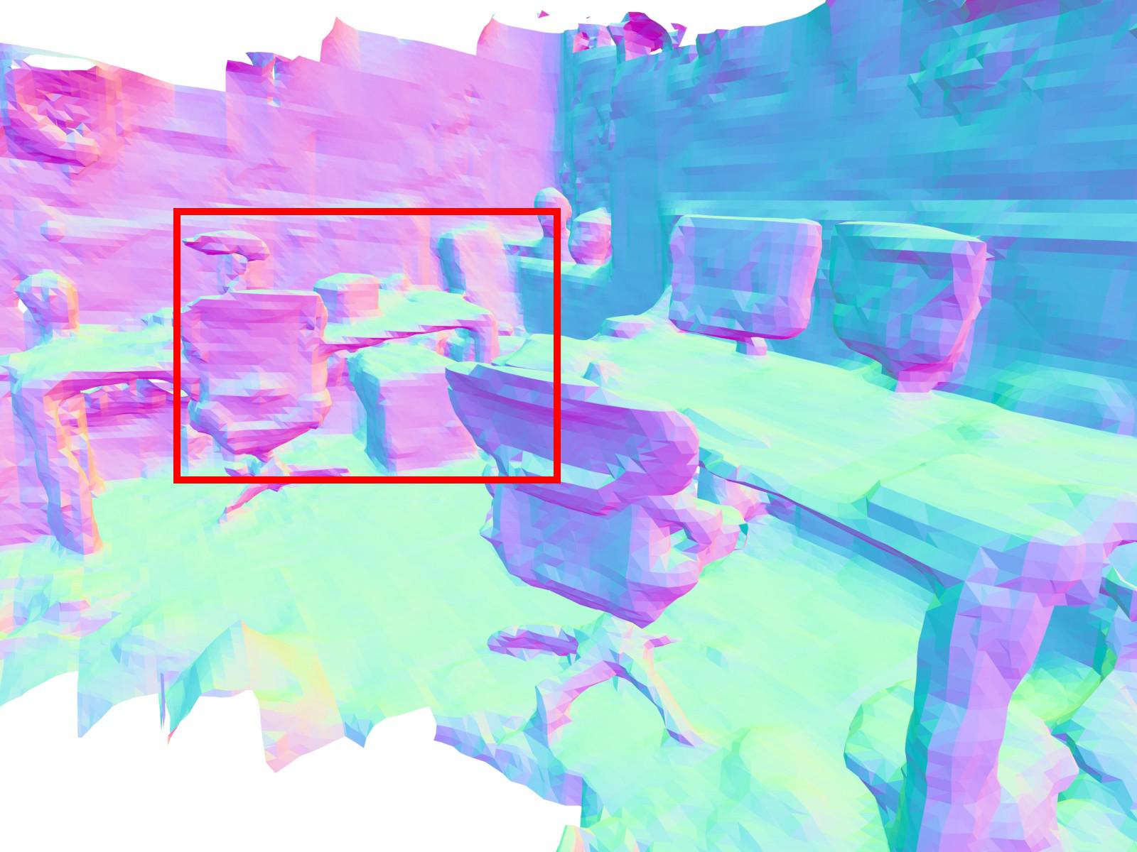
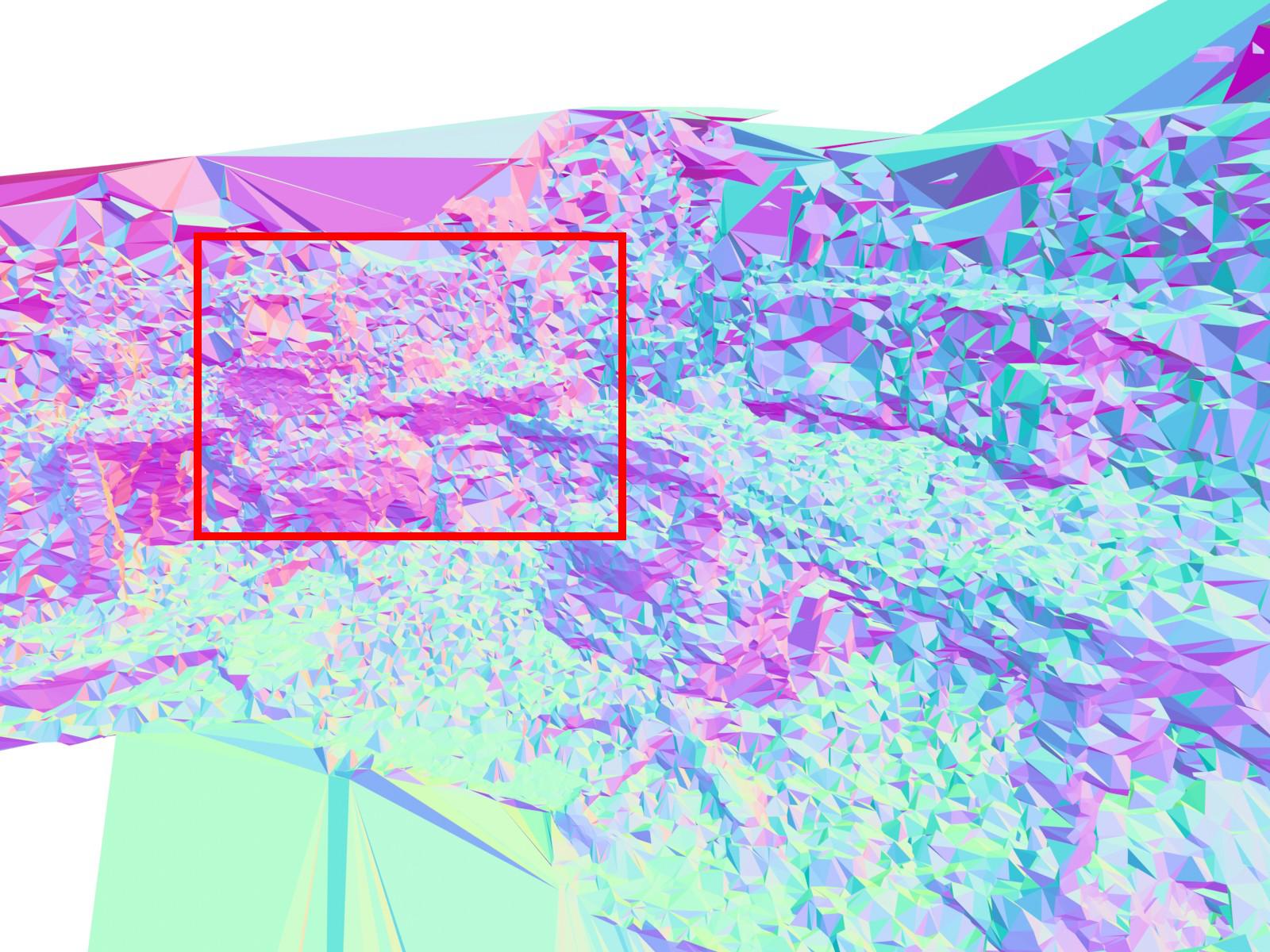
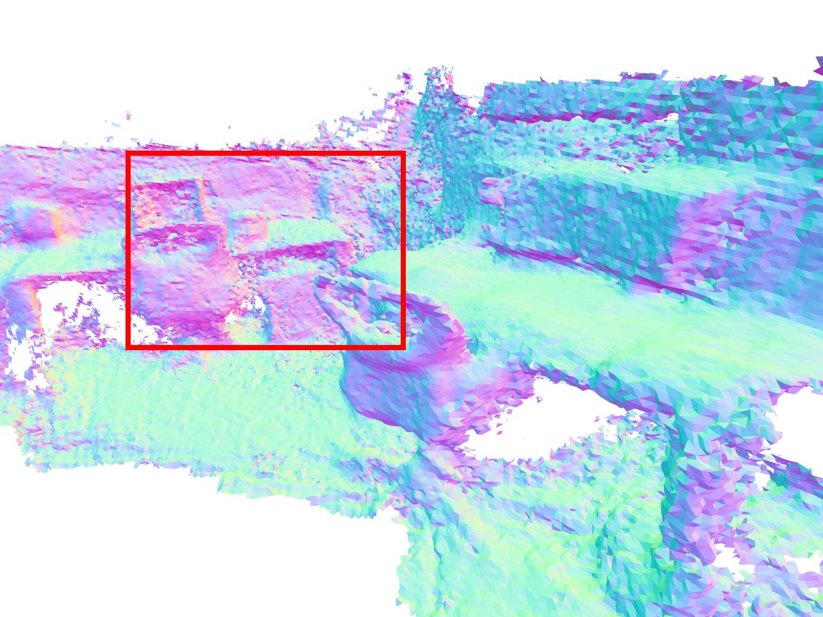
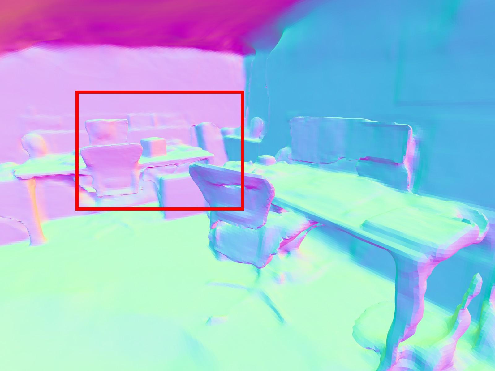
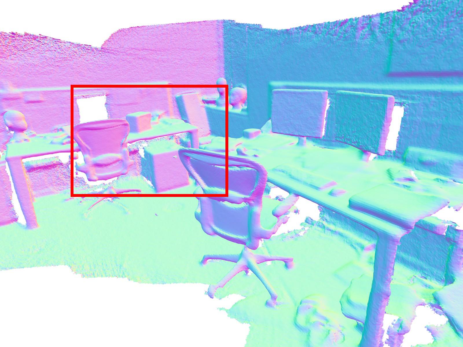
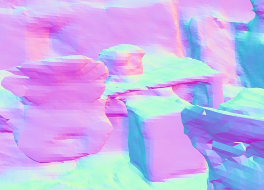
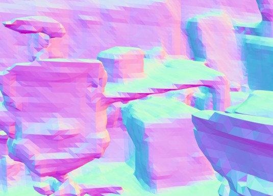
NICE-SLAM	Vox-Fusion	COLMAP	DROID-SLAM	NICER-SLAM	GT
RGB-D input		RGB input

Figure 5: 3D Reconstruction Results on the 7-Scenes Dataset [48]. The second row shows zoomed-in normal maps. It is apparent that the quality of the scene representation is substantially worse for the other RGB-based methods despite their better tracking accuracy.

It is worth noting that even with the less accurate camera poses from our tracking pipeline, our results in novel view synthesis are notably better than all baseline methods including those using additional depth inputs, see Table 4 and Fig. 4. On the one hand, the methods using traditional representations like COLMAP and DROID-SLAM suffer from rendering missing regions in the 3D reconstruction, and their renderings tend to be noisy. On the other hand, neural-implicit based approaches like NICE-SLAM and Vox-Fusion can fill in those missing areas but their renderings are normally over-smooth. We can faithfully render high-fidelity novel views even when those views are far from the training views. This illustrates the effectiveness of different losses for disambiguating the optimization of our scene representations.

	chess	fire	heads	office	pumpkin	kitchen	stairs	Avg.
RGB-D input
NICE-SLAM	2.16	1.63	7.80	5.73	19.34	3.31	4.31	6.33
Vox-Fusion	2.53	1.91	1.94	5.26	15.33	2.79	3.40	4.74
RGB input
COLMAP	3.42	2.40	1.70	10.42	52.32	5.08	2.62	11.14
DROID-SLAM	3.36	2.40	1.43	9.19	16.46	4.94	1.85	5.66
DROID-SLAM∗	3.55	2.49	3.32	10.93	48.53	4.72	2.58	10.87
NICER-SLAM	3.28	6.85	4.16	10.84	20.00	3.94	10.81	8.55

Table 4: Camera Tracking Results on the 7-Scenes Dataset [48]. ATE RMSE [cm] ($\downarrow$) is used as the evaluation metric.

Evaluation on 7-Scenes [48]

We also evaluate on the challenging real-world dataset 7-Scenes to benchmark the robustness of different methods when the input images are of low resolutions and have severe motion blurs. For geometry illustrated in Fig. 5, we can notice that NICER-SLAM produces sharper and more detailed geometry over all baselines. In terms of tracking, as can be observed in Table 4, baselines with RGB-D input outperform RGB-only methods overall, indicating that the additional depth inputs play an essential role for tracking especially when RGB images are imperfect. Among RGB-only methods, COLMAP and DROID-SLAM* (without global bundle adjustment) perform poorly in the pumpkin scene because it contains large textureless and reflective regions in the RGB sequence. NICER-SLAM is more robust to such issues thanks to the predicted monocular geometric priors.

4.2 Ablation Study

To support our design choices, we investigate the effectiveness of different losses, the hierarchical architecture, SDF-density transformation, as well as the comparison between SDF and occupancy.

Losses

We first verify the effectiveness of different losses for the mapping process from Sec. 3.3. In Table 4.2 (a), we evaluate both 3D reconstruction and tracking because we conduct local BA on the third stage of mapping. As can be noticed, using all losses together leads to the best overall performance. Without monocular depth or normal loss, both mapping and tracking accuracy drops significantly, indicating that these monocular geometric cues are important for the disambiguation of the optimization process.

Hierarchical Architecture

In Table 4.2 (b) we compare our proposed scene representations to two variations. The first one is to remove the multi-resolution color feature grids $\{\Phi_{l}^{\text{color}}\}_{1}^{L}$ and only represent scene colors with the MLP $f^{\text{color}}$. This change leads to large performance drops on all metrics, showing the necessity of having multi-res feature grids for colors. The second variation is to remove the coarse feature grid $\Phi^{\text{coarse}}$ and uses only fine-level feature grids to represent SDFs. This also causes inferior performance, especially in the completeness/completeness ratio, indicating that the coarse feature grid can indeed help to learn geometry better.

SDF-to-Density Transformation

We also compare different design choices for the transformation from SDF to volume density (see Sec. 3.2): (a) Fixed $\beta$ value, (b) globally optimizable $\beta$ as in [68], and also (c) different voxel size for counting (our default setting uses $64^{3}$). As can be seen in Table 4.2 (c), with the locally adaptive transformation and under the chosen voxel size, our method is able to obtain both better scene geometry and camera tracking.

SDF vs. Occupancy

Unlike recent implicit-based dense SLAM systems [51, 76, 67] which use occupancy to implicitly represent scene geometry, we instead use SDFs. To verify this design choice, we keep the architecture identical but only replace the output in Eq. (4) to let the occupancy probability be between 0 and 1. The Eikonal loss $\mathcal{L}_{\text{eikonal}}$ is also removed. In Fig. 6 we compare reconstruction results with given GT poses, and can clearly see that using SDFs leads to more accurate geometry.

Table 5: Ablation Study. On a single randomly selected Replica scene (office-4), we evaluate both camera tracking and reconstruction. Best results are highlighted asfirst,second, andthird.

(a) Ablation Study on Losses in Eq. (16). ATE RMSE$\downarrow$ Acc. $\downarrow$ Comp. $\downarrow$ Comp. Ratio $\uparrow$ Normal Cons. $\uparrow$ w/o $\{\Phi_{l}^{\text{color}}\}^{L}_{1}$ 9.92 8.32 8.49 50.13 87.84 w/o $\Phi^{\text{coarse}}$ 3.07 4.51 5.11 67.29 90.17 Ours 2.01 3.03 3.87 83.98 90.96 (b) Ablation Study on Hierarchical Architecture. ATE RMSE$\downarrow$ Acc. $\downarrow$ Comp. $\downarrow$ Comp. Ratio $\uparrow$ Normal Cons. $\uparrow$ Fixed $\beta$=0.01 3.81 7.77 8.28 39.48 87.52 Fixed $\beta$=0.001 3.98 3.48 5.05 76.67 90.39 Global optim. $\beta$ 2.62 3.64 4.53 76.35 90.88 Voxel size $32^{3}$ 3.00 3.19 4.35 81.90 90.65 Voxel size $128^{3}$ 2.16 4.35 4.87 68.96 90.40 Ours 2.01 3.03 3.87 83.98 90.96 (c) Ablation Study on SDF-to-Density Transformation.

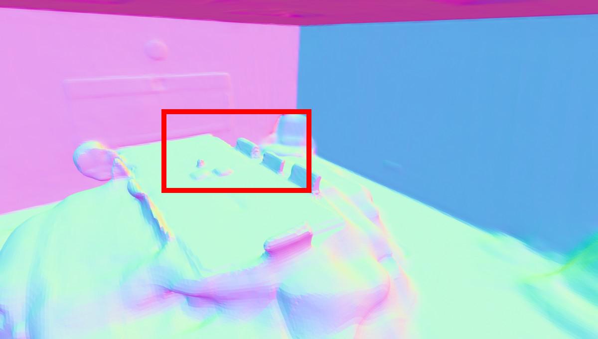
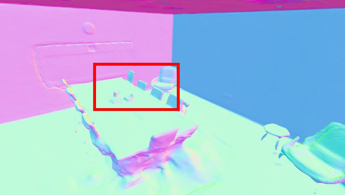
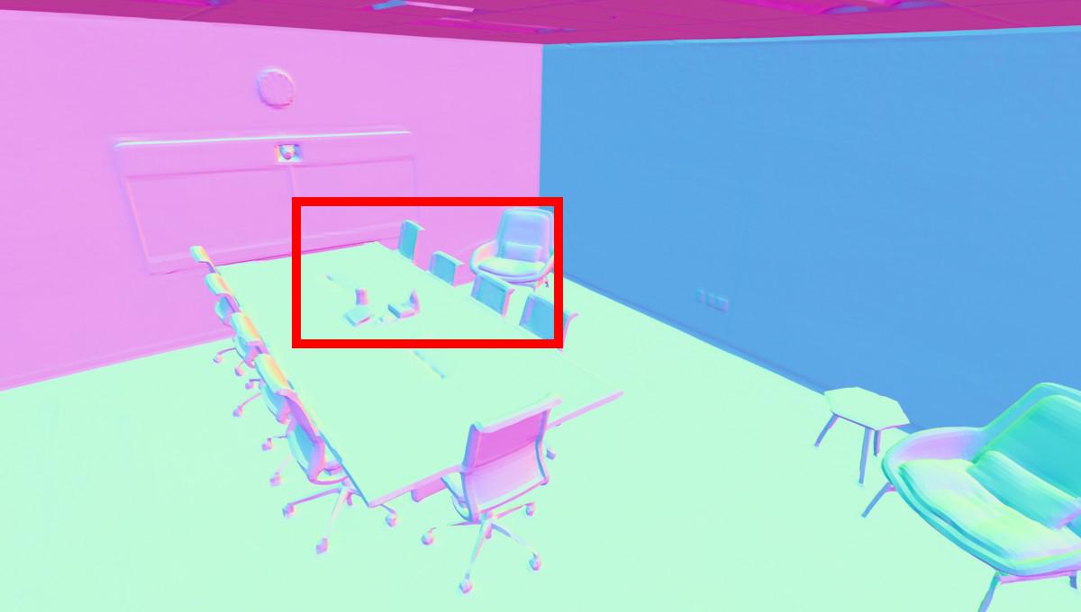
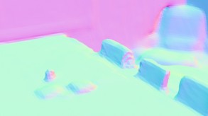
w/ Occupancy	w/ SDF	GT

Figure 6: Ablation Study on SDF vs. Occupancy. We conduct the ablation on one random Replica scene (office-4). The second row depicts zoomed-in normal maps for better comparison.

5 Conclusions

We present NICER-SLAM, a novel dense RGB SLAM system that is end-to-end optimizable for both neural implicit map representations and camera poses. We show that additional supervisions from easy-to-obtain monocular cues e.g. depths, normals, and optical flows can enable our system to reconstruct high-fidelity 3D dense maps and learn high-quality scene colors accurately and robustly in large indoor scenes.

Limitations

Although we show benefits over SLAM methods using traditional scene representations in terms of mapping and novel view synthesis, our pipeline is not yet optimized to be real-time. Also, no loop closure is performed under the current pipeline so the tracking performance should be further improvable.

Acknowledgements

This project is partially supported by the SONY Research Award Program and a research grant by FIFA. The authors thank the Max Planck ETH Center for Learning Systems (CLS) for supporting Songyou Peng and the strategic research project ELLIIT for supporting Viktor Larsson. We thank Weicai Ye, Boyang Sun, Jianhao Zheng, and Heng Li for their helpful discussion.

References

- [1] Wenjing Bian, Zirui Wang, Kejie Li, Jia-Wang Bian, and Victor Adrian Prisacariu. Nope-nerf: Optimising neural radiance field with no pose prior. arXiv preprint arXiv:2212.07388, 2022.
- [2] Michael Bloesch, Jan Czarnowski, Ronald Clark, Stefan Leutenegger, and Andrew J. Davison. Codeslam - learning a compact, optimisable representation for dense visual SLAM. In Proc. IEEE Conf. on Computer Vision and Pattern Recognition (CVPR), pages 2560–2568, 2018.
- [3] Erik Bylow, Jürgen Sturm, Christian Kerl, Fredrik Kahl, and Daniel Cremers. Real-time camera tracking and 3d reconstruction using signed distance functions. In Robotics: Science and Systems (RSS), volume 2, page 2, 2013.
- [4] Zhiqin Chen and Hao Zhang. Learning implicit fields for generative shape modeling. In Proc. IEEE Conf. on Computer Vision and Pattern Recognition (CVPR), pages 5939–5948, 2019.
- [5] Julian Chibane, Thiemo Alldieck, and Gerard Pons-Moll. Implicit functions in feature space for 3d shape reconstruction and completion. In Proc. IEEE Conf. on Computer Vision and Pattern Recognition (CVPR), pages 6970–6981, 2020.
- [6] Shin-Fang Chng, Sameera Ramasinghe, Jamie Sherrah, and Simon Lucey. Gaussian activated neural radiance fields for high fidelity reconstruction and pose estimation. In Proc. of the European Conf. on Computer Vision (ECCV), pages 264–280. Springer, 2022.
- [7] Chi-Ming Chung, Yang-Che Tseng, Ya-Ching Hsu, Xiang-Qian Shi, Yun-Hung Hua, Jia-Fong Yeh, Wen-Chin Chen, Yi-Ting Chen, and Winston H Hsu. Orbeez-slam: A real-time monocular visual slam with orb features and nerf-realized mapping. arXiv preprint arXiv:2209.13274, 2022.
- [8] Ronald Clark. Volumetric bundle adjustment for online photorealistic scene capture. In Proc. IEEE Conf. on Computer Vision and Pattern Recognition (CVPR), pages 6124–6132, 2022.
- [9] Jan Czarnowski, Tristan Laidlow, Ronald Clark, and Andrew J Davison. Deepfactors: Real-time probabilistic dense monocular slam. IEEE Robotics and Automation Letters, 5(2):721–728, 2020.
- [10] Angela Dai, Matthias Nießner, Michael Zollhöfer, Shahram Izadi, and Christian Theobalt. Bundlefusion: Real-time globally consistent 3d reconstruction using on-the-fly surface reintegration. ACM Trans. on Graphics, 36(4):1, 2017.
- [11] François Darmon, Bénédicte Bascle, Jean-Clément Devaux, Pascal Monasse, and Mathieu Aubry. Improving neural implicit surfaces geometry with patch warping. In Proc. IEEE Conf. on Computer Vision and Pattern Recognition (CVPR), pages 6260–6269, 2022.
- [12] Ainaz Eftekhar, Alexander Sax, Jitendra Malik, and Amir Zamir. Omnidata: A scalable pipeline for making multi-task mid-level vision datasets from 3d scans. In Proc. of the IEEE International Conf. on Computer Vision (ICCV), pages 10786–10796, 2021.
- [13] Jakob Engel, Vladlen Koltun, and Daniel Cremers. Direct sparse odometry. IEEE Trans. on Pattern Analysis and Machine Intelligence (PAMI), 40(3):611–625, 2017.
- [14] Daniel Girardeau-Montaut. Cloudcompare. France: EDF R&D Telecom ParisTech, 11, 2016.
- [15] Amos Gropp, Lior Yariv, Niv Haim, Matan Atzmon, and Yaron Lipman. Implicit geometric regularization for learning shapes. arXiv preprint arXiv:2002.10099, 2020.
- [16] Michael Grupp. evo: Python package for the evaluation of odometry and slam. https://github.com/MichaelGrupp/evo, 2017.
- [17] Chiyu Jiang, Avneesh Sud, Ameesh Makadia, Jingwei Huang, Matthias Nießner, and Thomas Funkhouser. Local implicit grid representations for 3d scenes. In Proc. IEEE Conf. on Computer Vision and Pattern Recognition (CVPR), pages 6001–6010, 2020.
- [18] Mohammad Mahdi Johari, Camilla Carta, and François Fleuret. Eslam: Efficient dense slam system based on hybrid representation of signed distance fields. arXiv preprint arXiv:2211.11704, 2022.
- [19] Georg Klein and David Murray. Parallel tracking and mapping for small ar workspaces. In IEEE International Symposium on Mixed and Augmented Reality (ISMAR), pages 225–234. IEEE, 2007.
- [20] Lukas Koestler, Nan Yang, Niclas Zeller, and Daniel Cremers. Tandem: Tracking and dense mapping in real-time using deep multi-view stereo. In Proc. Conf. on Robot Learning (CoRL), pages 34–45. PMLR, 2022.
- [21] Evgenii Kruzhkov, Alena Savinykh, Pavel Karpyshev, Mikhail Kurenkov, Evgeny Yudin, Andrei Potapov, and Dzmitry Tsetserukou. Meslam: Memory efficient slam based on neural fields. In 2022 IEEE International Conference on Systems, Man, and Cybernetics (SMC), pages 430–435. IEEE, 2022.
- [22] Heng Li, Xiaodong Gu, Weihao Yuan, Luwei Yang, Zilong Dong, and Ping Tan. Dense rgb slam with neural implicit maps. In Proc. of the International Conf. on Learning Representations (ICLR), 2023.
- [23] C. Lin, W. Ma, A. Torralba, and S. Lucey. Barf: Bundle-adjusting neural radiance fields. In Proc. of the IEEE International Conf. on Computer Vision (ICCV), 2021.
- [24] Stefan Lionar, Daniil Emtsev, Dusan Svilarkovic, and Songyou Peng. Dynamic plane convolutional occupancy networks. In Proc. of the IEEE Winter Conference on Applications of Computer Vision (WACV), pages 1829–1838, 2021.
- [25] Daniil Lisus and Connor Holmes. Towards open world nerf-based slam. arXiv preprint arXiv:2301.03102, 2023.
- [26] Shaohui Liu, Yinda Zhang, Songyou Peng, Boxin Shi, Marc Pollefeys, and Zhaopeng Cui. Dist: Rendering deep implicit signed distance function with differentiable sphere tracing. In Proc. IEEE Conf. on Computer Vision and Pattern Recognition (CVPR), pages 2019–2028, 2020.
- [27] William E Lorensen and Harvey E Cline. Marching cubes: A high resolution 3d surface construction algorithm. ACM siggraph computer graphics, 21(4):163–169, 1987.
- [28] Lars Mescheder, Michael Oechsle, Michael Niemeyer, Sebastian Nowozin, and Andreas Geiger. Occupancy networks: Learning 3d reconstruction in function space. In Proc. IEEE Conf. on Computer Vision and Pattern Recognition (CVPR), pages 4460–4470, 2019.
- [29] Ben Mildenhall, Pratul P Srinivasan, Matthew Tancik, Jonathan T Barron, Ravi Ramamoorthi, and Ren Ng. Nerf: Representing scenes as neural radiance fields for view synthesis. In Proc. of the European Conf. on Computer Vision (ECCV), 2020.
- [30] Yuhang Ming, Weicai Ye, and Andrew Calway. idf-slam: End-to-end rgb-d slam with neural implicit mapping and deep feature tracking. arXiv preprint arXiv:2209.07919, 2022.
- [31] Thomas Müller, Alex Evans, Christoph Schied, and Alexander Keller. Instant neural graphics primitives with a multiresolution hash encoding. ACM Trans. on Graphics, 41(4), 2022.
- [32] Raul Mur-Artal, Jose Maria Martinez Montiel, and Juan D Tardos. Orb-slam: a versatile and accurate monocular slam system. IEEE transactions on robotics, 31(5):1147–1163, 2015.
- [33] Raul Mur-Artal and Juan D Tardós. Orb-slam2: An open-source slam system for monocular, stereo, and rgb-d cameras. IEEE transactions on robotics, 33(5):1255–1262, 2017.
- [34] R. A. Newcombe, S. Izadi, O. Hilliges, D. Molyneaux, D. Kim, A. J. Davison, P. Kohi, J. Shotton, S. Hodges, and A. Fitzgibbon. Kinectfusion: Real-time dense surface mapping and tracking. In IEEE International Symposium on Mixed and Augmented Reality (ISMAR), 2011.
- [35] Richard A Newcombe, Steven J Lovegrove, and Andrew J Davison. Dtam: Dense tracking and mapping in real-time. In Proc. of the IEEE International Conf. on Computer Vision (ICCV), pages 2320–2327. IEEE, 2011.
- [36] M. Niemeyer, L. Mescheder, M. Oechsle, and A. Geiger. Differentiable volumetric rendering: Learning implicit 3D representations without 3D supervision. In Proc. IEEE Conf. on Computer Vision and Pattern Recognition (CVPR), 2019.
- [37] Matthias Nießner, Michael Zollhöfer, Shahram Izadi, and Marc Stamminger. Real-time 3d reconstruction at scale using voxel hashing. ACM Trans. on Graphics, 32(6):1–11, 2013.
- [38] Michael Oechsle, Songyou Peng, and Andreas Geiger. Unisurf: Unifying neural implicit surfaces and radiance fields for multi-view reconstruction. In Proc. of the IEEE International Conf. on Computer Vision (ICCV), pages 5589–5599, 2021.
- [39] Joseph Ortiz, Alexander Clegg, Jing Dong, Edgar Sucar, David Novotny, Michael Zollhoefer, and Mustafa Mukadam. isdf: Real-time neural signed distance fields for robot perception. In Robotics: Science and Systems (RSS), 2022.
- [40] Jeong Joon Park, Peter Florence, Julian Straub, Richard Newcombe, and Steven Lovegrove. Deepsdf: Learning continuous signed distance functions for shape representation. In Proc. IEEE Conf. on Computer Vision and Pattern Recognition (CVPR), pages 165–174, 2019.
- [41] Songyou Peng, Chiyu Jiang, Yiyi Liao, Michael Niemeyer, Marc Pollefeys, and Andreas Geiger. Shape as points: A differentiable poisson solver. Advances in Neural Information Processing Systems (NeurIPS), 34:13032–13044, 2021.
- [42] Songyou Peng, Michael Niemeyer, Lars Mescheder, Marc Pollefeys, and Andreas Geiger. Convolutional occupancy networks. In Proc. of the European Conf. on Computer Vision (ECCV), pages 523–540. Springer, 2020.
- [43] René Ranftl, Katrin Lasinger, David Hafner, Konrad Schindler, and Vladlen Koltun. Towards robust monocular depth estimation: Mixing datasets for zero-shot cross-dataset transfer. IEEE Trans. on Pattern Analysis and Machine Intelligence (PAMI), 2020.
- [44] Christian Reiser, Songyou Peng, Yiyi Liao, and Andreas Geiger. Kilonerf: Speeding up neural radiance fields with thousands of tiny mlps. In Proc. of the IEEE International Conf. on Computer Vision (ICCV), pages 14335–14345, 2021.
- [45] Antoni Rosinol, John J Leonard, and Luca Carlone. Nerf-slam: Real-time dense monocular slam with neural radiance fields. arXiv preprint arXiv:2210.13641, 2022.
- [46] J. L. Schonberger and J. M. Frahm. Structure-from-motion revisited. In Proc. IEEE Conf. on Computer Vision and Pattern Recognition (CVPR), 2016.
- [47] Thomas Schöps, Torsten Sattler, and Marc Pollefeys. BAD SLAM: bundle adjusted direct RGB-D SLAM. In Proc. IEEE Conf. on Computer Vision and Pattern Recognition (CVPR), pages 134–144. Computer Vision Foundation / IEEE, 2019.
- [48] Jamie Shotton, Ben Glocker, Christopher Zach, Shahram Izadi, Antonio Criminisi, and Andrew Fitzgibbon. Scene coordinate regression forests for camera relocalization in rgb-d images. In Proceedings of the IEEE conference on computer vision and pattern recognition, pages 2930–2937, 2013.
- [49] J. Straub, T. Whelan, L. Ma, Y. Chen, E. Wijmans, S. Green, J. J. Engel, R. Mur-Artal, C. R., S. Verma, A. Clarkson, M. Yan, B. Budge, Y. Yan, X. Pan, J. Yon, Y. Zou, K. Leon, N. Carter, J. Briales, T. Gillingham, E. Mueggler, L. Pesqueira, M. Savva, D. Batra, H. M. Strasdat, R. D. Nardi, M. Goesele, S. Lovegrove, and R. Newcombe. The Replica dataset: A digital replica of indoor spaces. arXiv preprint arXiv:1906.05797, 2019.
- [50] Jürgen Sturm, Nikolas Engelhard, Felix Endres, Wolfram Burgard, and Daniel Cremers. A benchmark for the evaluation of rgb-d slam systems. In Proc. IEEE International Conf. on Intelligent Robots and Systems (IROS), 2012.
- [51] Edgar Sucar, Shikun Liu, Joseph Ortiz, and Andrew J Davison. imap: Implicit mapping and positioning in real-time. In Proc. of the IEEE International Conf. on Computer Vision (ICCV), pages 6229–6238, 2021.
- [52] Edgar Sucar, Kentaro Wada, and Andrew Davison. Nodeslam: Neural object descriptors for multi-view shape reconstruction. In Proc. of the International Conf. on 3D Vision (3DV), pages 949–958. IEEE, 2020.
- [53] Towaki Takikawa, Joey Litalien, Kangxue Yin, Karsten Kreis, Charles Loop, Derek Nowrouzezahrai, Alec Jacobson, Morgan McGuire, and Sanja Fidler. Neural geometric level of detail: Real-time rendering with implicit 3d shapes. In Proc. IEEE Conf. on Computer Vision and Pattern Recognition (CVPR), pages 11358–11367, 2021.
- [54] Matthew Tancik, Pratul Srinivasan, Ben Mildenhall, Sara Fridovich-Keil, Nithin Raghavan, Utkarsh Singhal, Ravi Ramamoorthi, Jonathan Barron, and Ren Ng. Fourier features let networks learn high frequency functions in low dimensional domains. In Advances in Neural Information Processing Systems (NeurIPS), 2020.
- [55] Chengzhou Tang and Ping Tan. Ba-net: Dense bundle adjustment network. In Proc. of the International Conf. on Learning Representations (ICLR), 2019.
- [56] Zachary Teed and Jia Deng. Deepv2d: Video to depth with differentiable structure from motion. In Proc. of the International Conf. on Learning Representations (ICLR), 2020.
- [57] Zachary Teed and Jia Deng. Droid-slam: Deep visual slam for monocular, stereo, and rgb-d cameras. In Advances in Neural Information Processing Systems, volume 34, pages 16558–16569, 2021.
- [58] Benjamin Ummenhofer, Huizhong Zhou, Jonas Uhrig, Nikolaus Mayer, Eddy Ilg, Alexey Dosovitskiy, and Thomas Brox. Demon: Depth and motion network for learning monocular stereo. In Proc. IEEE Conf. on Computer Vision and Pattern Recognition (CVPR), pages 5038–5047, 2017.
- [59] Peng Wang, Lingjie Liu, Yuan Liu, Christian Theobalt, Taku Komura, and Wenping Wang. Neus: Learning neural implicit surfaces by volume rendering for multi-view reconstruction. arXiv preprint arXiv:2106.10689, 2021.
- [60] Zhou Wang, Alan C Bovik, Hamid R Sheikh, and Eero P Simoncelli. Image quality assessment: from error visibility to structural similarity. IEEE transactions on image processing, 13(4):600–612, 2004.
- [61] Z. Wang, S. Wu, W. Xie, M. Chen, and V. A. Prisacariu. Nerf–: Neural radiance fields without known camera parameters. arXiv preprint arXiv:2102.07064, 2021.
- [62] Thomas Whelan, Michael Kaess, Maurice Fallon, Hordur Johannsson, John Leonard, and John McDonald. Kintinuous: Spatially extended kinectfusion. In RSS ’12 Workshop on RGB-D: Advanced Reasoning with Depth Cameras, 2012.
- [63] Thomas Whelan, Stefan Leutenegger, Renato Salas-Moreno, Ben Glocker, and Andrew Davison. Elasticfusion: Dense slam without a pose graph. In Robotics: Science and Systems (RSS), 2015.
- [64] Xiuchao Wu, Jiamin Xu, Zihan Zhu, Hujun Bao, Qixing Huang, James Tompkin, and Weiwei Xu. Scalable neural indoor scene rendering. ACM Transactions on Graphics (TOG), 41(4):1–16, 2022.
- [65] Yiheng Xie, Towaki Takikawa, Shunsuke Saito, Or Litany, Shiqin Yan, Numair Khan, Federico Tombari, James Tompkin, Vincent Sitzmann, and Srinath Sridhar. Neural fields in visual computing and beyond. In Computer Graphics Forum, volume 41, pages 641–676. Wiley Online Library, 2022.
- [66] Haofei Xu, Jing Zhang, Jianfei Cai, Hamid Rezatofighi, and Dacheng Tao. Gmflow: Learning optical flow via global matching. In Proc. IEEE Conf. on Computer Vision and Pattern Recognition (CVPR), pages 8121–8130, 2022.
- [67] Xingrui Yang, Hai Li, Hongjia Zhai, Yuhang Ming, Yuqian Liu, and Guofeng Zhang. Vox-fusion: Dense tracking and mapping with voxel-based neural implicit representation. In IEEE International Symposium on Mixed and Augmented Reality (ISMAR), pages 499–507. IEEE, 2022.
- [68] Lior Yariv, Jiatao Gu, Yoni Kasten, and Yaron Lipman. Volume rendering of neural implicit surfaces. In Advances in Neural Information Processing Systems (NeurIPS), volume 34, pages 4805–4815, 2021.
- [69] Lior Yariv, Yoni Kasten, Dror Moran, Meirav Galun, Matan Atzmon, Basri Ronen, and Yaron Lipman. Multiview neural surface reconstruction by disentangling geometry and appearance. In Advances in Neural Information Processing Systems (NeurIPS), volume 33, pages 2492–2502, 2020.
- [70] L. Yen-Chen, P. Florence, J. T. Barron, A. Rodriguez, P. Isola, and T. Lin. iNeRF: Inverting neural radiance fields for pose estimation. In IEEE/RSJ International Conference on Intelligent Robots and Systems (IROS), 2021.
- [71] Zehao Yu, Songyou Peng, Michael Niemeyer, Torsten Sattler, and Andreas Geiger. Monosdf: Exploring monocular geometric cues for neural implicit surface reconstruction. Advances in Neural Information Processing Systems (NeurIPS), 2022.
- [72] K. Zhang, G. Riegler, N. Snavely, and V. Koltun. NERF++: Analyzing and improving neural radiance fields. 2020.
- [73] Richard Zhang, Phillip Isola, Alexei A Efros, Eli Shechtman, and Oliver Wang. The unreasonable effectiveness of deep features as a perceptual metric. In Proc. IEEE Conf. on Computer Vision and Pattern Recognition (CVPR), pages 586–595, 2018.
- [74] Shuaifeng Zhi, Michael Bloesch, Stefan Leutenegger, and Andrew J Davison. Scenecode: Monocular dense semantic reconstruction using learned encoded scene representations. In Proc. IEEE Conf. on Computer Vision and Pattern Recognition (CVPR), pages 11776–11785, 2019.
- [75] Huizhong Zhou, Benjamin Ummenhofer, and Thomas Brox. Deeptam: Deep tracking and mapping. In Proc. of the European Conf. on Computer Vision (ECCV), pages 822–838, 2018.
- [76] Zihan Zhu, Songyou Peng, Viktor Larsson, Weiwei Xu, Hujun Bao, Zhaopeng Cui, Martin R. Oswald, and Marc Pollefeys. Nice-slam: Neural implicit scalable encoding for slam. In Proc. IEEE Conf. on Computer Vision and Pattern Recognition (CVPR), pages 12786–12796, 2022.