DSAC: Low-Cost Rowhammer Mitigation Using In-DRAM Stochastic and Approximate Counting Algorithm

Abstract

DRAM has scaled to achieve low cost per bit and this scaling has decreased Rowhammer threshold which is the threshold number of activations for Rowhammer-induced bit-flip. Rowhammer has been a security threat for the entire system since this hardware-fault can be exploited by software-level attack. Thus, DRAM has adopted Target-Row-Refresh (TRR) which refreshes victim rows that can possibly lose stored data due to neighboring aggressor rows. Accordingly, prior works focused on TRR algorithm that can identify the most frequently accessed row, Rowhammer, to detect the victim rows. TRR algorithm can be implemented in memory controller, yet it can cause either insufficient or excessive number of TRRs due to lack of information of Rowhammer threshold and it can also degrade system performance due to additional command for Rowhammer mitigation. Therefore, this paper focuses on in-DRAM TRR algorithm.

In general, counter-based detection algorithms have higher detection accuracy and scalability compared to probabilistic detection algorithms. However, modern DRAM extremely limits the number of counters for TRR algorithm. This paper demonstrates that decoy-rows are the fundamental reason the state-of-the-art counter-based algorithms cannot properly detect Rowhammer under the area limitation. Decoy-rows are rows whose number of accesses does not exceed the number of Rowhammer accesses within an observation period. Thus, decoy-rows should not replace Rowhammer which are in a count table. Unfortunately, none of the state-of-the-art counter-based algorithms filter out decoy-rows. Consequently, decoy-rows replace Rowhammer in a count table and dispossess TRR opportunities from victim rows. Therefore, this paper proposes ‘in-DRAM Stochastic and Approximate Counting (DSAC) algorithm’, which leverages Stochastic Replacement to filter out decoy-rows and Approximate Counting for low area cost. The key idea is that a replacement occurs if a new row comes in more than a minimum count row in a count table on average so that decoy-rows cannot replace Rowhammer in a count table.

This paper proposes a Rowhammer protection index named Maximum Disturbance which measures the maximum accumulated number of row activations within an observation period. The experimental data show that DSAC can achieve 49x lower Maximum Disturbance than the state-of-the-art counter-based algorithm.

I Introduction

DRAM is a volatile memory since it stores data in a cell that consists of one capacitor and one transistor. However, DRAM manufacturers have scaled to achieve low cost per bit and this cell shrinkage has aggravated electromagnetic crosstalks between cells. This crosstalk has negative effects on row activation which must be preceded in order for system to write or read the data. The negative effects are activation-induced bit-flip. In fact, Intel claims that Samsung’s commodity DRAM is vulnerable to frequent row activations in 2012. Since then, the first academic paper [27] discussed this phenomenon and many researches [5, 13, 14, 29, 32, 45, 48, 51, 52, 53, 55, 57] on Rowhammer have presented bit-flip mechanisms and malicious bit-flip methods. Various TRR algorithms to mitigate Rowhammer disturbance on neighboring victim rows have also been proposed [56, 59, 30, 24, 25, 40, 46, 47]. However, a recent study [11] demonstrated that Rowhammer is still a problem and this can be aggravated since shrinking DRAM cell-to-cell distance decreases Rowhammer threshold (RH${}_{\text{TH}}$) which is the threshold number of activations for Rowhammer-induced bit-flip.

In Section III, the fundamental mechanisms of two activation-induced bit-flips are discussed. This paper categorizes activation-induced bit-flips into two types according to their relative activation time. One is Passing Gate Effect and the other is Rowhammer. Passing Gate Effect occurs when activation time is longer than the minimum time prescribed by memory standard specification, whereas Rowhammer occurs when activation time is the minimum prescribed time.

In Section IV, a critical feature in memory standard specification for Rowhammer mitigation is discussed. Memory standard specification must be considered for TRR algorithm to be practical and operate in real system. For low-power and high-command-bandwidth system operation, DRAM supports a feature called MR4 which can control refresh command interval. Unfortunately, MR4 is unfavorable to Rowhammer mitigation since it can decrease the chance of being mitigated by normal refresh operation and can compel detection algorithm to have an immense number of counters.

In Section V, the problem of state-of-the-art counter-based algorithms is discussed and the solution is proposed. This paper demonstrates the state-of-the-are counter-based algorithms cannot protect Rowhammer due to decoy-rows. Decoy-rows are rows whose number of accesses does not exceed the number of Rowhammer accesses within an observation period. As a result, decoy-rows replace Rowhammer which are in a count table and dispossess TRR chances from victim rows. Therefore, this paper proposes DSAC which can filter out decoy-rows by adopting Stochastic Replacement. The key idea is that a replacement occurs if a new row comes in more than a minimum count row in a count table on average. Since the number of decoy-row accesses cannot exceed the number of Rowhammer accesses within an observation period, decoy-rows cannot replace Rowhammer which are in a count table. This paper also proposes Time-Weighted Counting to mitigate Passing Gate Effect which counts more for a row that is activated longer than the minimum activation time prescribed by memory standard specification.

This paper makes the following key contributions:

• This paper contributes a comprehensive understanding of two activation-induced bit-flips: one is Passing Gate Effect and the other is Rowhammer.

• This paper proposes the first Passing Gate Effect mitigation mechanism named Time-Weighted Counting that can give different weights to each row depending on its activation time.

• This paper proposes Rowhammer mitigation mechanism named DSAC that can filter out decoy-rows and demonstrates that decoy-rows can degrade detection performance of the state-of-the-art counter-based algorithms under the area limitation and memory standard specification.

II Background

In this section, this paper describes the necessary background on DRAM organization and operation. For further detail, this paper refers the reader to prior studies on DRAM [27, 56, 11, 17, 18, 16, 19, 20, 21, 61].

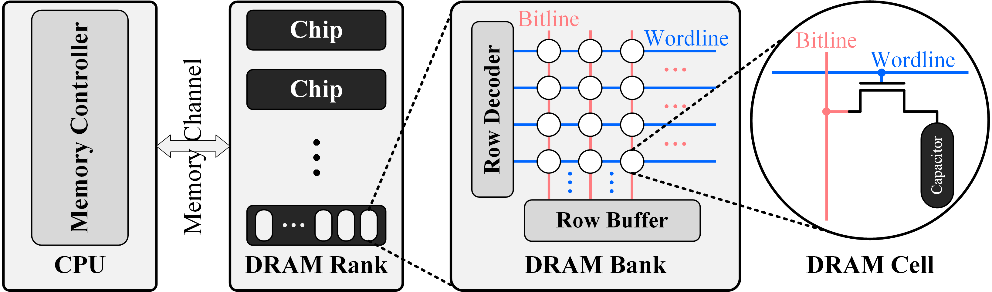
Figure 1: Architecture of a Typical DRAM-Based System

Figure 1 represents a typical computer architecture with emphasis on DRAM. DRAM stores data within cells that each consist of a single capacitor and a transistor. Since the transistor leaks its current, the capacitor leaks its charge over time. To prevent this cell data loss, DRAM cells need to be periodically refreshed. Thus, memory controller periodically issues refresh commands to DRAM.

A bank comprises many subarrays and each subarray contains a two-dimensional array of DRAM cells arranged in rows and columns. When accessing each cell, the row decoder first decodes incoming row address to open the row by driving the corresponding wordline. To write or read the stored data in DRAM cells, each row needs to be in an active state. The row must be precharged before further accesses can be made to other rows of the same bank.

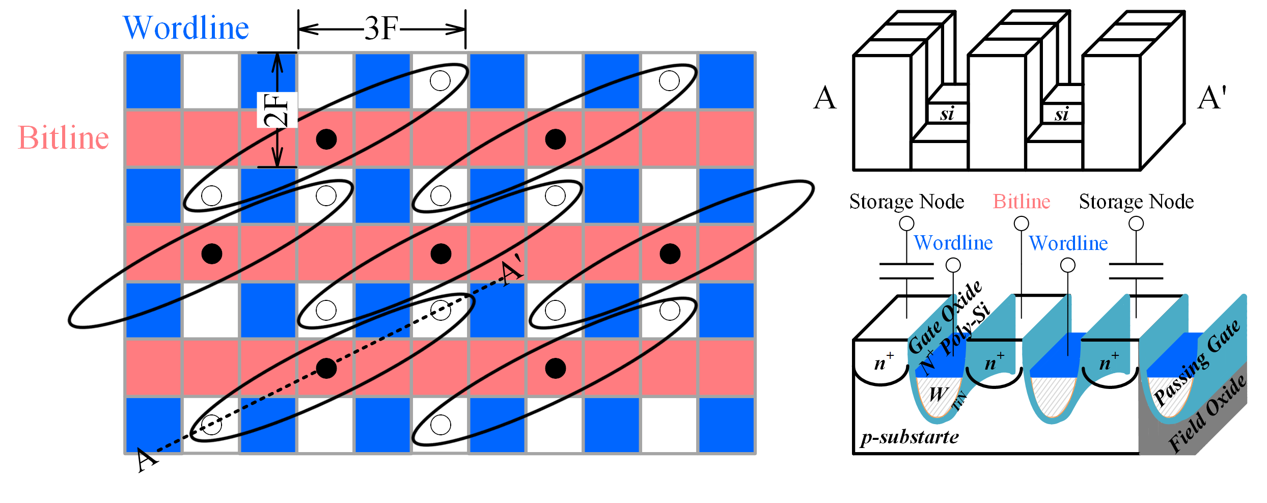
Figure 2: Physical Cell Layout of Modern DRAM

Figure 2 represents modern DRAM’s $6\text{F}^{2}$ physical cell layout [43, 10], where F represents area of 1 transistor and 1 capacitor. Buried wordline which is the gate of transistor that passes below the silicon surface level is adopted for cell shrinkage [43, 53]. The three-dimensional view of Figure 2 depicts saddle-fin transistor structure and it is adopted for improving data write-time and overcoming Short Channel Effect which is a side effect of cell shrinkage that can decrease transistor’s threshold voltage [23, 26, 39, 57]. The field oxide region is called Shallow Trench Isolation region and wordline in this region is called passing gate [58, 39].

III Bit-Flip Mechanism

Bit-Flip. Since new generations of DRAM scale down cell-to-cell distance for low cost per bit, electromagnetic interactions between cells can be increased. This noise has negative effects on row activation which can lead to activation-induced bit-flip. This paper categorizes activation-induced bit-flips into two types according to their relative activation time. One is Passing Gate Effect and the other is Rowhammer. Passing Gate Effect occurs when activation time is longer than the minimum time prescribed by memory standard specification, whereas Rowhammer occurs when activation time is the minimum prescribed time.

Passing Gate Effect. When a passing gate is activated for a long period of time, it acts as an aggressor row that can flip the data of neighboring victim rows. This phenomenon is called Passing Gate Effect.

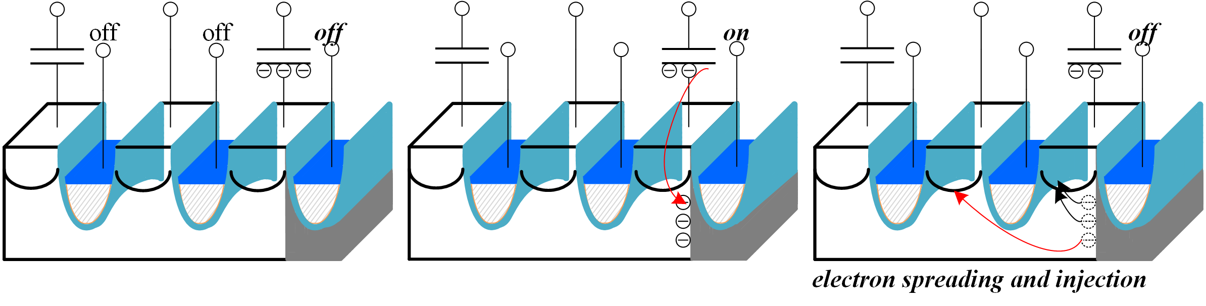
Figure 3: Physical Level Bit-flip Mechanism of Stored Data 0

Figure 3 depicts a bit-flip mechanism of initial cell data 0. If a passing gate is activated for a long period of time, it can attract electrons from the capacitor. After the long activation is finished, these electrons can be spread and injected into silicon substrate. Repeating this process can cause data 0 to be flipped. Therefore, long activation time can increase the possibility of bit-flip.

Rowhammer. When a row is frequently activated, it acts as an aggressor row that can flip the data of neighboring victim rows. This phenomenon is called Rowhammer. In terms of Passing Gate Effect, how long a row is activated is critical. In terms of Rowhammer, how often a row is activated is critical.

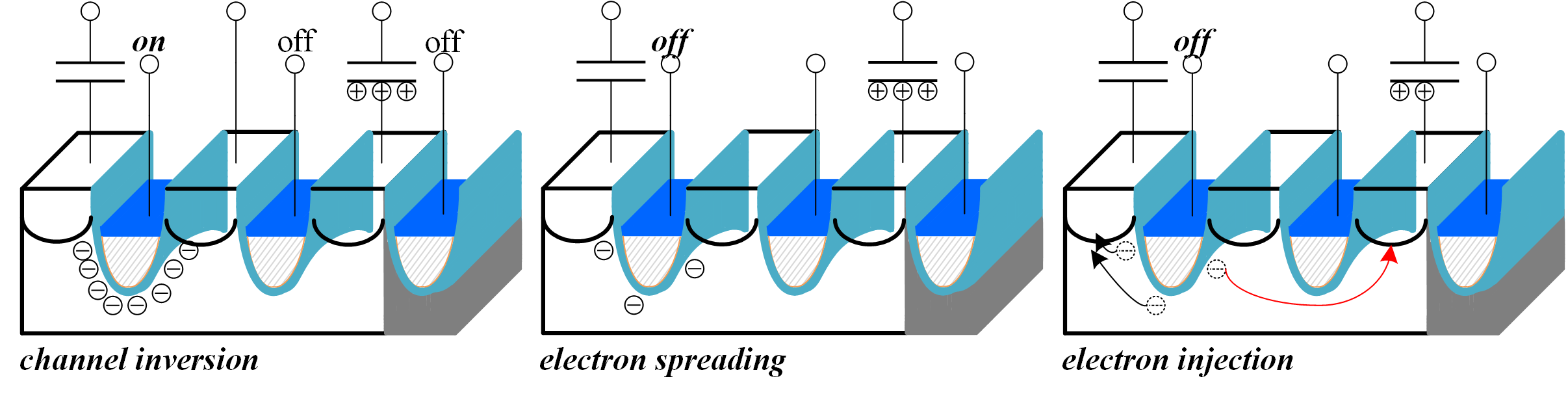
Figure 4: Physical Level Bit-flip Mechanism of Stored Data 1

Figure 4 depicts bit-flip mechanism of initial cell data 1. If a row is activated, electrons gather around transistor’s channel which is the phenomenon called Channel Inversion. After the row activation is finished, these electrons can be spread out and some of the electrons can be injected into neighboring cell’s capacitor. Repeating this process can cause data 1 to be flipped. Therefore, short activation time for frequent activation can increase the possibility of bit-flip.

IV Rowhammer Vulnerability in System

IV-A System-Level Security

Hardware-fault attacks typically requires physical-level access to the device. However, Rowhammer is a hardware-fault that can be exploited by software-level attack. According to various researches that demonstrate Rowhammer vulnerability on servers, mobile systems, virtual machines, browsers, JavaScript, and network [55, 52, 51, 48, 45, 42, 14, 13, 5, 2, 32], Rowhammer is a nuisance for the entire system.

In order to prevent Rowhammer, TRR algorithm that can identify the most frequently accessed row is necessary so that victim rows can be precisely labeled for Target-Row-Refresh (TRR). Memory controller-based TRR indicates that TRR algorithms is implemented solely in memory controller while memory controller-aided TRR indicates that in-DRAM TRR algorithm is supported by memory controller.

IV-B Memory Controller-Perspective TRR

Memory Controller-Based TRR. TRR algorithm can be implemented solely in memory controller. However, it can cause either insufficient or excessive number of TRRs due to lack of information of RH${}_{\text{TH}}$ since DRAM manufacturers do not supply any data related to semiconductor process. Insufficient number of TRRs can lead to Rowhammer-induced bit-flip and excessive number of TRRs can degrade system performance due to additional command for Rowhammer mitigation.

Memory Controller-Aided TRR. In-DRAM TRR algorithm can be supported by memory controller and features such as RFM according to [22] are being considered in the industry. However, it can degrade system performance due to additional operation for Rowhammer mitigation. Additionally, memory controller-aided TRR can lead to TRR-induced bit-flip caused by TRR algorithm clash between DRAM and memory controller.

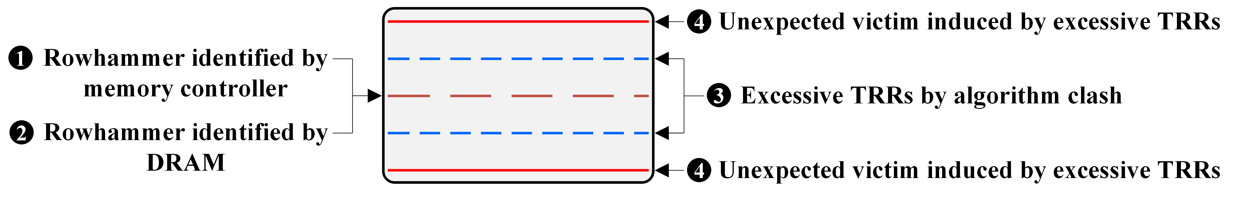
Figure 5: TRR-Induced Bit-Flip Caused by TRR Algorithm Clash

Figure 5 depicts bit-flip mechanism induced by TRR algorithm clash. If both memory controller and DRAM adopt the same TRR algorithm, then they can identify the same row as Rowhammer. As a result, neighboring rows can be excessively TRRed. This excessive TRRs can produce unexpected victim rows.

To summarize, TRR algorithm can be implemented in memory controller, yet it can cause either insufficient or excessive number of TRRs due to lack of information of RH${}_{\text{TH}}$ and it can also degrade system performance due to additional command for Rowhammer mitigation. Therefore, this paper focuses on in-DRAM TRR algorithm.

IV-C Memory Standard Specification

Memory standard specification must be considered for TRR algorithm to be practical and operate in real system. Since memory controller cannot perform any other operation while DRAM is refreshed, refresh operation degrades system performance. In addition to system performance degradation, refresh operation requires high power consumption.

To alleviate these negative impacts, DRAM supports a feature called MR4 which can control refresh command interval. Unfortunately, MR4 is unfavorable to Rowhammer mitigation since it can decrease the chance of being mitigated by normal refresh operation and can compel detection algorithm to have an immense number of counters.

MR4. MR4 can allow memory controller to increase refresh command interval. Due to this increased refresh command interval, power consumption on refresh operation can be decreased and command bandwidth can be increased.

According to memory standard specifications [17, 18, 16, 19, 20, 21], the time interval of two refresh commands is defined as tREFI and DRAM must refresh all cells in 8K refresh commands. This 8K refresh commands window is defined as tREFW. Hence, tREFW is equivalent to $\text{8K}\times\text{tREFI}$. Typical tREFW is 32ms for 8K refresh commands. Accordingly, tREFI is 3.9us (32ms/8K). Thus, all cells must be refreshed in 32ms using 8K refresh commands. Note that the nominal value of tREFI and tREFW can differ for LPDDR, DDR, GDDR, and HBM.

However, MR4 can control tREFI by multiplying a parameter prescribed by memory standard specification. This parameter ranges from 0.5x to 4x. If a parameter is 1x, then effective tREFI (tREFIe) is equal to $1\times\text{tREFI}$. Since tREFW is equivalent to $\text{8K}\times\text{tREFI}$, effective tREFW (tREFWe) is equal to $1\times\text{tREFW}$. If a parameter is 4x, then tREFIe is equal to $4\times\text{tREFI}$ and tREFWe is equal to $4\times\text{tREFW}$ which corresponds to 15.6us and 128ms, respectively. Figure 6 illustrates tREFIe corresponding to different MR4. Note that tRFC represents actual refresh operation time which does not allow any other commands and tRC represents active command interval.

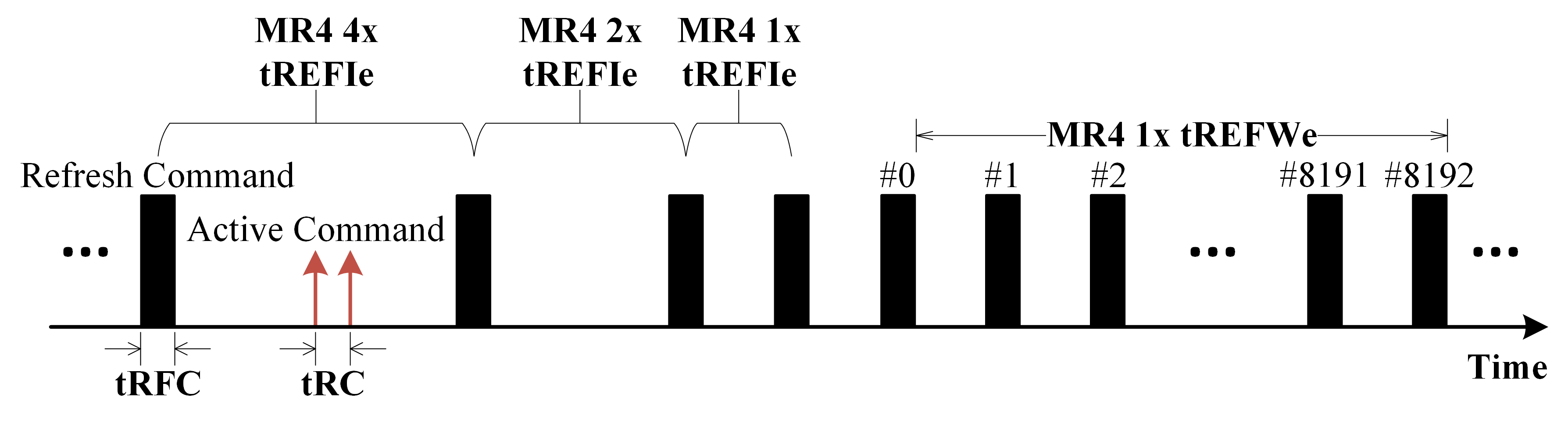
Figure 6: Refresh Command Interval Corresponding to Different MR4

While MR4 can be favorable to system, it can be unfavorable to Rowhammer mitgation since increased tREFWe can decrease the chance of being mitigated by normal refresh operation which is a regular refresh operation for preventing cell data loss.

MPA. As shown in Figure 6, MR4 can increase the maximum possible number of row activations (MPA) in tREFWe. For example, MPA of MR4 4x is approximately four times higher than MPA of MR4 1x. MPA in tREFWe (MPA${}_{\text{tREFWe}}$) can be calculated by Equality 1 where tRCmin is the minimum active command interval prescribed by memory standard specification.

$$\centering\mathrm{MPA_{tREFWe}=\frac{tREFIe-tRFC}{tRCmin}\times{8K}}\@add@centering$$ (1)

Since the number of Rowhammer attacks can be increased when MPA${}_{\text{tREFWe}}$ is increased, MR4 is unfavorable to Rowhammer mitigation. Nevertheless, if DRAM can possess the number of counters for TRR algorithm equal to the number of rows per bank, then all the row activations can be precisely counted and DRAM can effortlessly detect Rowhammer.

TABLE I: Baseline Parameters

  Parameter Description Value tREFIe Effective Ref. CMD Interval 15.625us (MR4 4x) tREFWe Effective 8K Ref. CMD Window 128ms (MR4 4x) tRFC Ref. Operation Time 280ns for 8Gb/Ch. LPDDR4 tRCmin Min. Act. CMD Interval 60ns (LPDDR4) MPA${}_{\text{tREFIe}}$ Max. # of Act. CMDs in tREFIe 255 (MR4 4x) MPA${}_{\text{tREFWe}}$ Max. # of Act. CMDs in tREFWe 2,095K (MR4 4x) RH${}_{\text{TH}}$ Th. # of Act. for RH-Induced Bit-Flip 20K [11] # of Rows/Bank # of Rows/Bank 64K (8Gb/Ch. LPDDR4) # of Banks Total # of Banks per Chip 8 (LPDDR4)  

According to Table I, if DRAM can reserve 64K counters for TRR algorithm, then there can be no error in counts and TRR algorithm can accurately identify Rowhammer. However, this requires DRAM to have 512K ($64\text{K}\times 8$) counters for all banks and it is impossible for DRAM to integrate those enormous bulk of circuits due to the area limitation. For example, the required area for 512K counters is equivalent to the area of 7 DRAM chips (512K Row Register$+$512K Row Counter$=$216,352,206$\text{um}^{2}$) according to Table II. While 512K counters can be reserved in DRAM cell array, it requires 9% area overhead and significant system performance overhead because read-modify-write operation is mandatory to update row activation count for every active, write, and read operation.

To summarize, system requires MR4 for the benefit of low-power and high-command-bandwidth system operation, yet MR4 makes it difficult for DRAM to mitigate Rowhammer since MR4 can decrease the chance of being mitigated by normal refresh and can compel detection algorithm to have an immense number of counters. Therefore, this paper proposes low-cost in-DRAM TRR algorithm named DSAC which can mitigate Rowhammer and Time-Weighted Counting which can mitigate Passing Gate Effect.

V DSAC

V-A Passing Gate Effect Countermeasure

Time-Weighted Counting. Since Passing Gate Effect can occur when a row is activated for a long period of time, row activation time prescribed by memory standard specification is a major factor. This row activation time is defined as tRAS and it ranges from 42ns to 70,200ns according to memory standard specification [17, 18].

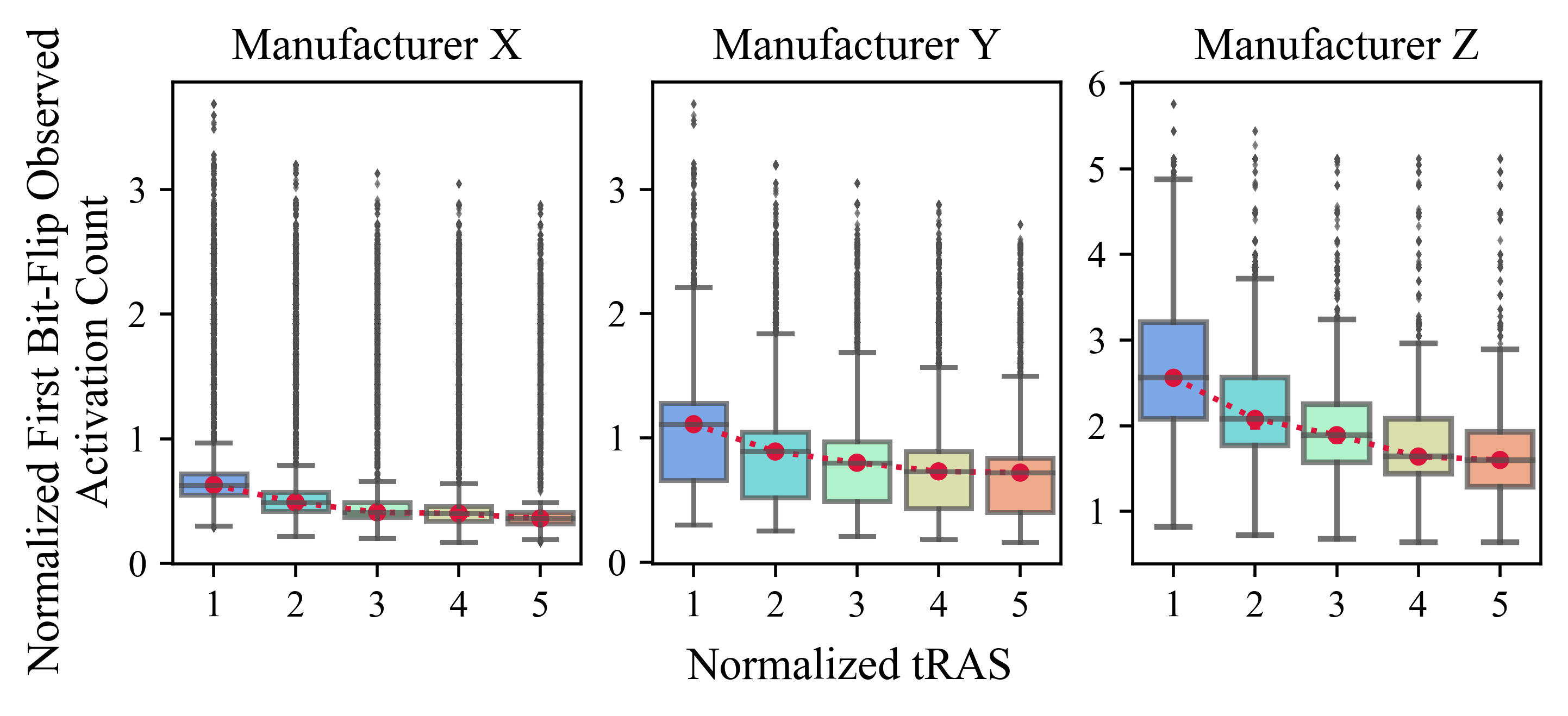
Figure 7: Bit-Flip Characteristic of Different tRAS

Figure 7 indicates the bit-flip characteristic of different tRAS from three major manufacturers’ DDR4 DRAM. The data show that longer tRAS decreases Passing Gate Effect-induced bit-flip threshold. However, it shows a non-linear relationship as the gradient gets gradual when tRAS gets longer. Therefore, this paper proposes the first Passing Gate Effect mitigation mechanism named Time-Weighted Counting. Time-Weighted Counting leverages the logarithmic function that can increase counter weight when tRAS is longer than tRASmin, yet its growth can slow down as tRAS gets longer as follows:

$$\centering W_{C}=\mathrm{\alpha\times\log_{2}\frac{tRAS}{tRASmin}}\@add@centering$$ (2)

, where $W_{C}$ is the counter weight for each row, and $\alpha$ is a weight parameter that can be fine-tuned. Note that if $\alpha$ is equal to 0, then Time-Weighted Counting is disabled. If $\alpha$ is greater than 0 and tRAS is equal to tRASmin, then $W_{C}$ becomes 0 and it does not give more weights to corresponding row. However, if $\alpha$ is greater than 0 and tRAS is equal to $2\times\text{tRASmin}$, then $W_{C}$ becomes $\alpha\times 1$ and this weight is added to corresponding row’s count value.

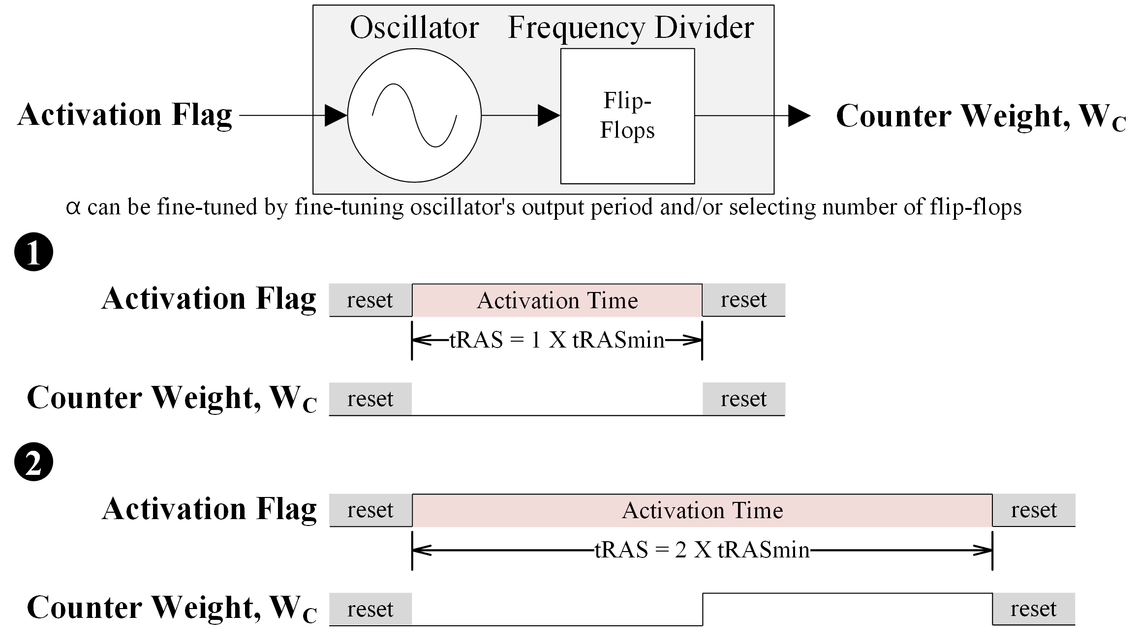
Figure 8: Hardware Implementation of Time-Weighted Counting

Figure 8 shows hardware implementation of Time-Weighted Counting. If DSAC’s row counter receives a row from memory controller, then it increments corresponding row’s count value. Simultaneously, the row counter can receive $W_{C}$ value for that row if tRAS is longer than tRASmin. For example, if $\alpha$ is 1 and tRAS is $2\times\text{tRASmin}$, then $W_{C}$ becomes 1 and corresponding row’s count value becomes 2 (1 for normal counting and 1 for Time-Weighted Counting). The complete architecture is discussed in Figure 16.

V-B Rowhammer Countermeasure

Since Rowhammer can occur when a row is frequently activated, row activation count is a major factor. Finding the most frequently appearing elements are an active research area such as data stream [1, 4, 6, 7, 9, 8, 12, 31, 33, 34, 36], cache replacement policy [41, 60], and network management [28, 15, 50, 3, 44]. State-of-the-art detection algorithms can be categorized into two types, counter-based and sketch-based. This paper focuses on counter-based algorithms for their low space complexity.

Approximate Counting. Among counter-based algorithms such as Frequent algorithm [37], Lossy Counting algorithm [35], and Space Saving algorithm [36], Space Saving algorithm is considered to be the best area-efficient detection algorithm [6, 7, 34, 1].

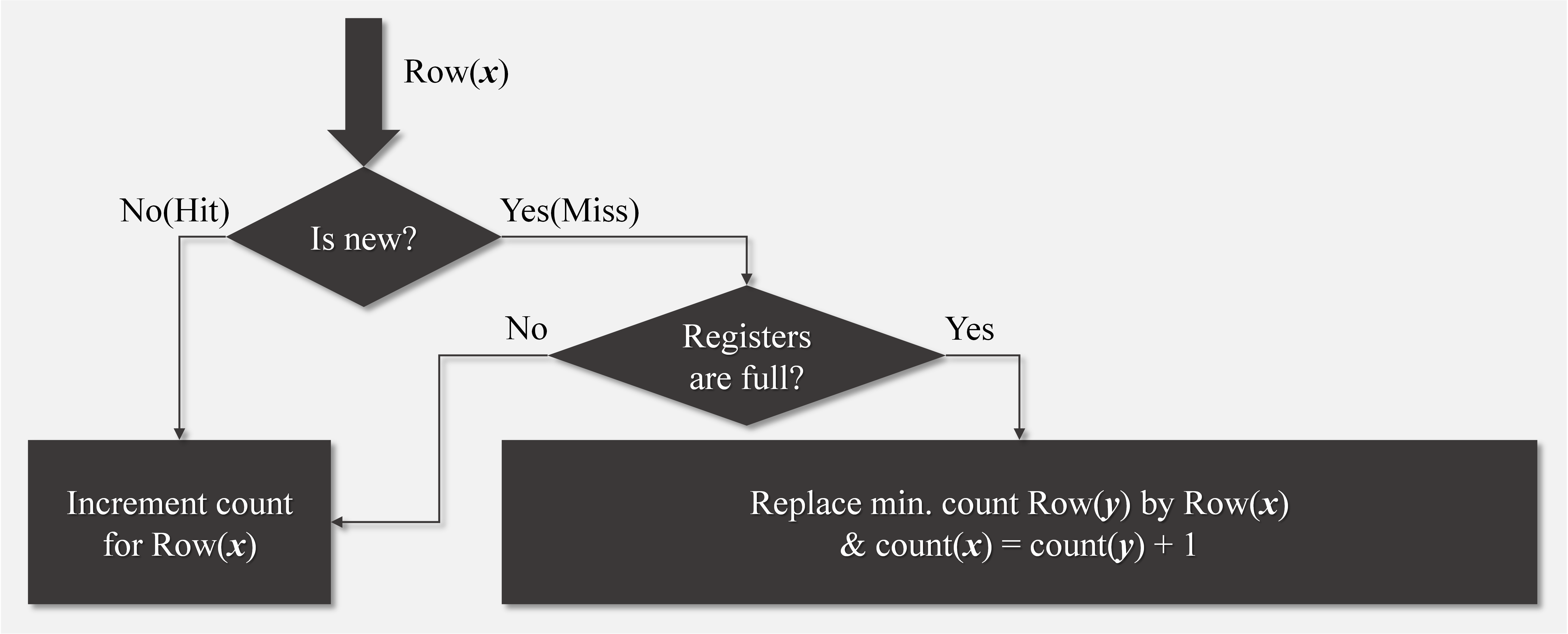
Figure 9: Flowchart of Space Saving Algorithm

• Hit: Increment the corresponding count value.

• Miss: Check if the count table is full.

• Insertion: If the count table is not full, then insert a new row into the count table and increments its count value.

• Replacement: If the count table is full, then a min. count row can be replaced by a new row. & increment min. count by 1.

Figure 9 represents the flowchart of Space Saving algorithm. Space Saving algorithm updates its count table on every incoming row. The key idea of Space Saving algorithm is that it keeps track of replaced row’s count so that it can approximate replaced row’s count value when replaced row returns into a count table. For example, if a minimum count row(y) is replaced by a new row(x), then count(x) becomes count(y)$+$1 instead of discarding count(y). Leveraging this Approximate Counting [36], Space Saving algorithm can be area-efficient.

However, all those state-of-the-art counter-based algorithms have a drawback on Rowhammer application. These detection algorithms are vulnerable to decoy-rows since DRAM severely limits the number of counters for TRR algorithm. Decoy-rows are rows whose number of accesses does not exceed the number of Rowhammer accesses within an observation period. Hence, decoy-rows should not be inserted into detection algorithm’s count table.

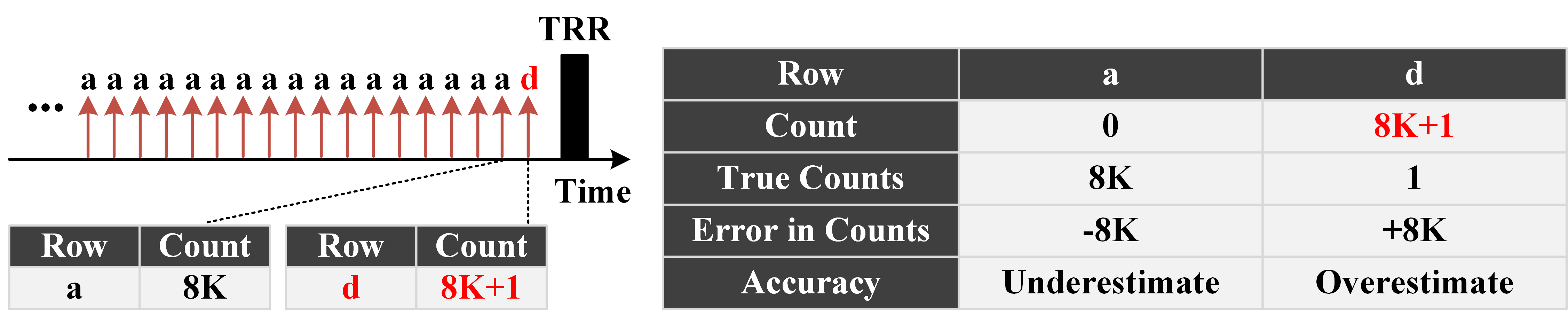
Figure 10: Problem of State-of-the-Art Counter-Based Algorithms

Figure 10 simplifies the drawback of Space Saving algorithm. The number of counters is 1 and TRR is performed on the black bar labeled as TRR. There are only two incoming rows, aggressor-row(a) and decoy-row(d). Since Space Saving algorithm updates its count table on every incoming row, decoy-row(d) takes all the count value of aggressor-row(a). In consequence, aggressor-row(a) is extremely underestimated and decoy-row(d) is extremely overestimated. Therefore, the victim rows of aggressor-row(a) cannot be TRRed which can lead to Rowhammer-induced bit-flip.

As shown in above, the detection performance of Space Saving algorithm strongly depends on the number of counters. The error in counts (Ce) can be represented as follows:

$$\centering Ce<\lfloor\frac{n}{c}\rfloor\@add@centering$$ (3)

, where n is the number of row activations and c is the number of counters. Note that Ce can be maximized when the number of rows is equal to the number of counters$+$1.

Stochastic Replacement. Based on the above analysis, this paper focuses on filtering decoy-rows to minimize Ce. Since the number of decoy-row accesses cannot exceed the number of Rowhammer accesses within an observation period, an algorithm that can filter out rows whose number of counts is lower than the number of Rowhammer accesses is required. Therefore, this paper proposes DSAC which can filter out decoy-rows by adopting Stochastic Replacement.

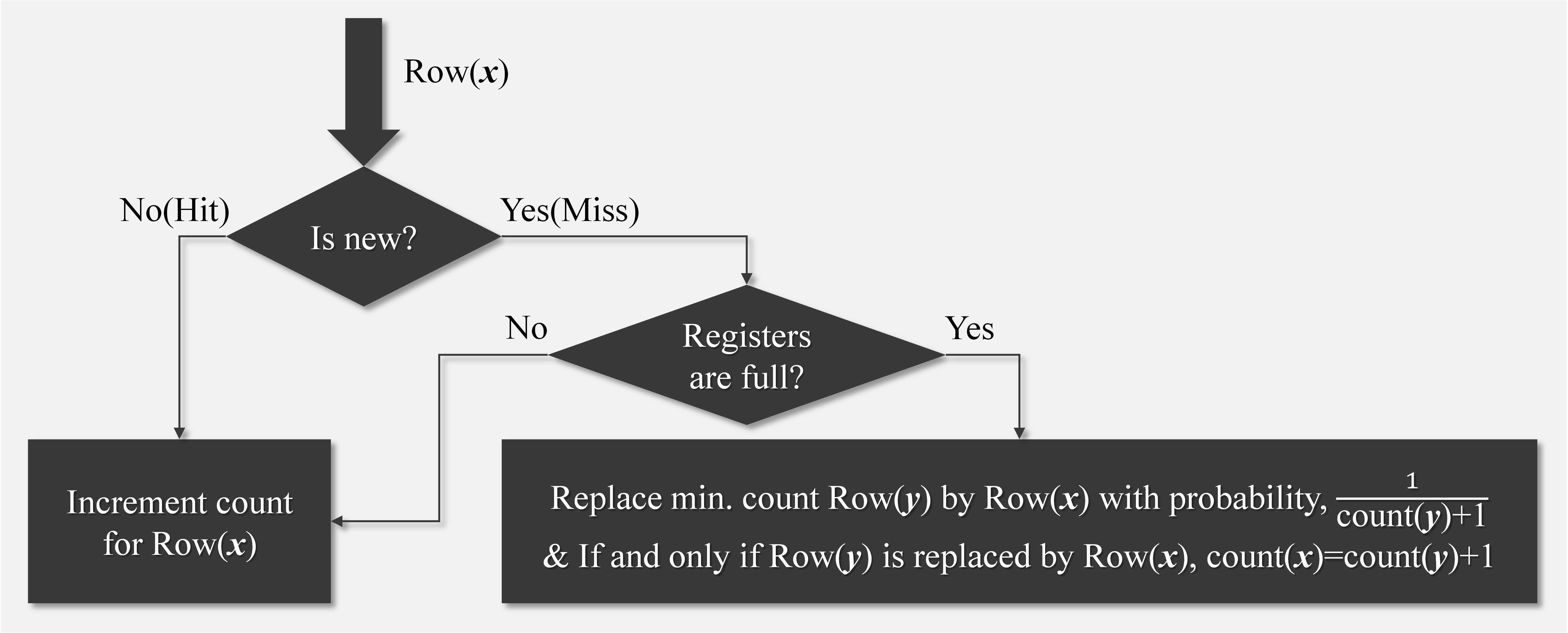
Figure 11: Flowchart of DSAC

• Hit: Increment the corresponding count value.

• Miss: Check if the count table is full.

• Insertion: If the count table is not full, then insert a new row into the count table and increments its count value.

• Replacement: If the count table is full, then a min. count row can be replaced by a new row with probability,

  $$\text{P}(r)=\frac{1}{\text{min. cnt}+1}$$ (4)

  , where min. cnt is the minimum count value in a count table. & Increment min. count by 1 iff replacement occurs.

Figure 11 represents the flowchart of DSAC. The key idea of DSAC is that a replacement occurs if a new row comes in more than a minimum count row in a count table on average. For example, a minimum count row(y) is replaced by a new row(x) with replacement probability, $\text{P}(r)=\frac{1}{\text{count}(y)+1}$. Thus, row(x) can be inserted into a count table if it comes in more than count(y)$+$1 stochastically. Noe that DSAC leverages Approximate Counting for area-efficiency by keeping track of replaced row’s count.

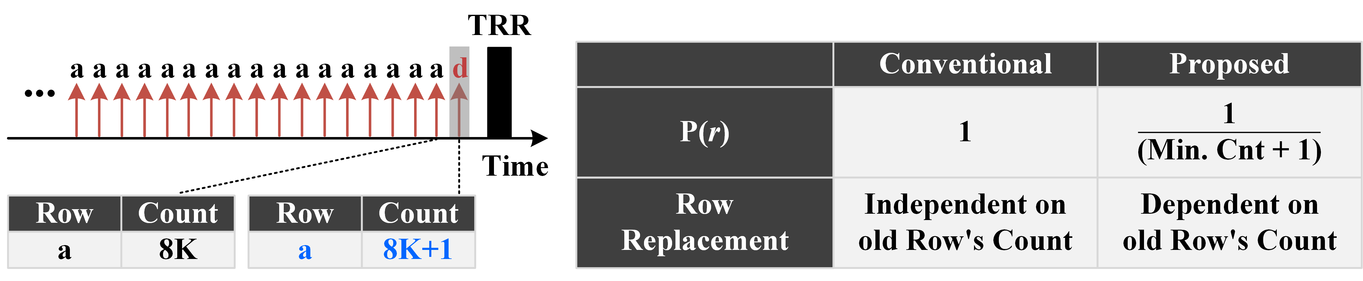
Figure 12: High-Level Overview of DSAC

Figure 12 simplifies how DSAC can solve the problem in Figure 10. Since $\text{P}(r)=\frac{1}{\text{8K}+1}$ is quite low, DSAC can keep aggressor-row(a) in a count table and can TRR neighboring victim rows. Consequently, DSAC can minimize Ce as follows:

$$\centering Ce\leq\lfloor\frac{\text{min. cnt}}{c}\rfloor\@add@centering$$ (5)

, where min. cnt is the minimum count value in a count table and c is the number of counters. Rigorous mathematical analysis can be found in Appendix DSAC: Low-Cost Rowhammer Mitigation Using In-DRAM Stochastic and Approximate Counting Algorithm and the experimental data in Section VII prove those arguments are valid.

Figure 13: Operation Example of 2 Count Table DSAC

Figure 13 illustrates how DSAC operates when the number of counters is equal to 2. The count table is full by row(a) and row(b) with minimum count value equal to 2. This sets P(r) equal to 1/(2$+$1), which is 33%. New row(c) does not replace old row(b). Hence, P(r) remains the same. New row(c) incomes again but still does not replace old row(b). Hence, P(r) remains the same. New row(c) replaces old RA(b). Hence, minimum count value is set to 3 and P(r) is set to 25%. Note that P(r) can be reset to 1 after TRR.

To summarize, in-DRAM Stochastic and Approximate Counting algorithm (DSAC) is proposed for filtering out decoy-rows with area-efficiency. Pseudocode of DSAC can be found in Algorithm 1.

// Hit

1 if incoming$\_$ROW == count$\_$table[i][‘ROW’] then

2      count$\_$table[i][‘CNT’] ++

3      return

// Miss

4 else

       // Insertion

5       if count$\_$table[i][‘ROW’] == None then

6            count$\_$table[i][‘ROW’] = Incoming$\_$ROW

7            count$\_$table[i][‘CNT’] ++

8            return

      // Replacement

9       else

10             i    = argmin${}_{\text{j}}$(count$\_$table[j][‘CNT’])

11             min$\_$cnt = min(count$\_$table[j][‘CNT’])

12             r    = RANDOM[0,1)

13             if r $\leq$ 1 / (min$\_$cnt + 1) then

14                  count$\_$table[i][‘ROW’] = Incoming$\_$ROW

15                  count$\_$table[i][‘CNT’] ++

16                  return

17            else

18                  return

19            

20      

Algorithm 1 Pseudocode of DSAC

Figure 14 illustrates operation of DSAC in detail.

Figure 14: Operation of DSAC in Detail

The black bars represent refresh commands whose interval is set by MR4. The red arrows represent active commands. The table represents DSAC’s count table. Assume that system operation commences at REF # 1. The count table is initialized with no rows and no count value. DSAC operates as a perfect tracker until the number of incoming rows reaches the number of counters since it can insert every rows into the count table.

When the number of incoming rows reaches the same number of counters, DSAC begins Stochastic Replacement and sets P(r) as 1/(min. cnt$+$1). According to the minimum count value which is equal to 5, P(r) is set to 1/(5$+$1).

Incoming row(n) is filtered out 5 times consecutively with P(r) equal to 1/6. Replacement occurs at the blue arrow and Approximate Counting sets the minimum count value equal to 5$+$1. According to the minimum count value which is equal to 6, P(r) is set to 1/(6$+$1).

Row(o) replaces row(n) at the blue arrow and the minimum count value is set to 6$+$1. Accordingly, P(r) is set to 1/(7$+$1). Row(o) comes in once more and the corresponding count value is incremented since row(o) is in the count table. Correspondingly, P(r) is set to 1/(8$+$1).

Since row(a), row(b), and row(o) are in the count table, their corresponding count values are incremented. Accordingly, the minimum count row changes from row(o) to row(k). However, P(r) remains the same as 1/9 since row(k)’s count value is 8. Row(o), row(a), and row(b) come again and their corresponding count values are incremented. A new row(p) comes in at the blue arrow and the minimum count value is set to 9. Thus, P(r) is set to 1/(9$+$1). Row(a), row(b), and row(p) come and their corresponding count values are incremented. Accordingly, the minimum count row changes from row(p) to row(j). However, P(r) remains the same as 1/(9$+$1) since row(j)’s count value is 9. Row(p) comes again and its corresponding count value is incremented.

REF_TRR${}_{\text{TH}}$ represents a refresh command that can be issued after DSAC reaches its predetermined TRR threshold (TRR${}_{\text{TH}}$). A row whose count value is the highest in the count table is considered to be Rowhammer (RH). Hence, corresponding victim rows are RH$+$x and RH$-$x, where x is non-negative integers. Therefore, RH$+$x and RH$-$x can be TRRed at REF_TRR${}_{\text{TH}}$. Note that normal refresh (N) can be performed with TRR if $\frac{\text{tRFC}}{\text{tRCmin}}$ is greater than the required number of activations for both N and TRR. In this case, the required number of activations for both N and TRR is equal to 3. Thus, if $\frac{\text{tRFC}}{\text{tRCmin}}$ is greater than 3, then N can be performed with TRR.

TRR Threshold. Since MR4 can increase MPA in tREFIe (MPA${}_{\text{tREFIe}}$) which can increase Rowhammer vulnerability as discussed in Section IV, TRR${}_{\text{TH}}$ should be adaptive to MPA${}_{\text{tREFIe}}$. Therefore, DSAC introduces adaptive TRR${}_{\text{TH}}$ which can change TRR${}_{\text{TH}}$ depending on MPA${}_{\text{tREFIe}}$, so that DSAC can mitigate double-sided hammer in system operation condition. Note that double-sided hammer occurs when a victim row is sandwiched in between two aggressor rows [11]. Consequently, the victim row requires to be TRRed before one of the aggressor rows reaches the count value equal to $\frac{\text{RH}_{\text{TH}}}{2}$.

Figure 15: Example of Adaptive TRR${}_{\text{TH}}$

Figure 15 depicts example of adaptive TRR${}_{\text{TH}}$. Flag for TRR${}_{\text{TH}}$ is triggered according to Inequality 6.

$$\centering\text{Sum of Counts in a Count Table}\geq\frac{\text{RH}_{\text{TH}}}{2}-\text{MPA}_{\text{tREFIe}}\@add@centering$$ (6)

According to Inequality 6, TRR${}_{\text{TH}}$ can be $\frac{\text{RH}_{\text{TH}}}{2}-256$ for MR4 4x. Note that different TRR${}_{\text{TH}}$ can also be adopted if necessary.

V-C Architecture of DSAC

Figure 16: Architecture of 4 Count Table DSAC with Time-Weighted Counter

Figure 16 shows architecture of DSAC equipped with Time-Weighted Counter. TRR module consists of TRR module controller and TRR row detector.

TRR Module Controller. TRR Module Controller generates control signals for TRR row detector.

MAX_OR_MIN is used to search the maximum count row or the minimum count row for every ACTIVE which indicates active command. ACTIVE comes with ACTIVE_ROW_[0:15] which indicates each bit of row address for 64K rows. When Max. or Min. Scheduler receives ACTIVE, MAX_OR_MIN is low and TRR Row Detector searches the minimum count row to store ACTIVE_ROW_[0:15] into a count table. However, STOCHASTIC_REPLACEMENT can block this operation. If STOCHASTIC_REPLACEMENT is low, then FILTERED_ROW_[0:15] is equal to ACTIVE_ROW_[0:15] and can be stored into a count table. If STOCHASTIC_REPLACEMENT is high, then FILTERED_ROW_[0:15] is filtered out. Once the minimum count row search is completed, MAX_OR_MIN becomes high and TRR Row Detector searches the maximum count row.

In order to generate STOCHASTIC_REPLACEMENT which can filter out decoy-rows, PRNG Seed Mixer, LFSR, Min. Count Register, and Probability LUT are implemented. PRNG Seed Mixer receives PUF which leverages DRAM’s Physical Unclonable Function so that its output SEED_MIXER_[0:19] can be unique to each DRAM. SEED_MIXER_[0:19] is updated for every tREFWe using ALL_CELL_REF_DONE which indicates all cells get refreshed so that LFSR’s PRBS_[0:19] cannot be readily deciphered. LFSR updates its output PRBS_[0:19] for every active command using ACTIVE in order to leverage probability for every ACTIVE_ROW_[0:15]. Min. Count Register receives all the row counts and outputs the minimum count MIN_CNT_[0:13] when MAX_OR_MIN is low. Probability LUT receives MIN_CNT_[0:13] and selects corresponding probability generated by utilizing PRBS_[0:19]. 20 bits are required to cover 2,095K MPA${}_{\text{tREFWe}}$.

PLUS_OR_MINUS is used to calculate victim rows for every TRR_FLAG which indicates refresh command that reaches TRR${}_{\text{TH}}$. When Plus or Minus Scheduler receives TRR_FLAG, PLUS_OR_MINUS is low and Victim Row Cal. in TRR Row Detector calculates RH$-$x. Once RH$-$x calculation is completed, PLUS_OR_MINUS becomes high and Victim Row Cal. in TRR Row Detector calculates RH$+$x. Note that x is non-negative integers to mitigate $\pm$x rows adjacent to aggressor row.

COUNTER_WEIGHT is used to mitigate Passing Gate Effect and it can increment count value for row that is activated longer than tRASmin.

TRR Row Detector. TRR Row Detector detects aggressor row RH_[0:15] and outputs victim rows VICTIM_[0:15]. The mechanism of TRR Row Detector is based on a single-elimination tournament where the loser of each match-up is eliminated from the tournament. Therefore, RH_[0:15] is the winner of the final match-up. Note that the number of counters is scalable.

When MAX_OR_MIN is low, Comparator # 0(1)’s output MAX_OR_MIN # 0(1) selects less count value between two Row Counters in Count MUX # 0(1). MAX_OR_MIN # 0 and MAX_OR_MIN # 1 are decoded to PNT_REG # 0/1/2/3. PNT_REG # 0/1/2/3 is used to control Row Register and corresponding Row Counter. Since MAX_OR_MIN is low, pointed Row Register replaces stored row by a new row and corresponding Row Counter increments its count. If all the count values are the same, then low index Row Register has a priority of replacement.

When MAX_OR_MIN is high, Comparator # 0(1)’s output MAX_OR_MIN # 0(1) selects greater count value between two Row Counters in Count MUX # 0(1). MAX_OR_MIN # 0 and MAX_OR_MIN # 1 are decoded to PNT_REG # 0/1/2/3. PNT_REG # 0/1/2/3 is used to control Row Register and corresponding Row Counter. Since MAX_OR_MIN is high, pointed Row Register sends its row to Rowhammer Register. Rowhammer Register outputs RH_[0:15] when MAX_OR_MIN # 2 is high. If all the count values are the same, then Rowhammer Register selects row from high index Row Register to consider temporal locality.

Row Counter is reset once TRR is performed. Note that if all the count values are 0, then no TRR is performed to save power consumption and TRR-induced bit-flip. Note that the number of counters is scalable.

TABLE II: Required Area for Each Module of DSAC

  Area Module (Description) $\text{um}^{2}$ % DRAM 1 Chip (Major Manufacturers’ 2nd Gen. 10nm 8Gb/Ch. LPDDR4) 32,510,639 100.000 Row Register (16 Bits for 64K Rows of 8Gb/Ch. LPDDR4) 251 0.001 Row Counter (14Bit for 20K RH${}_{\text{TH}}$ [11]) 162 0.000 Comparator (14 Bits for Comparing Each Bit of 2 Counters) 166 0.001 2-to-1 Multiplexer (14 MUXs for Selecting Each Bit of 2 Counters) 125 0.000 Decoder (Pointing Max. Cnt Row Reg. or Min. Cnt Row Reg.) 536 0.002 Rowhammer Register (16 Bits for 16Bit Row Register) 251 0.001 Victim Row Cal. (Full Adder for Calculating Victim Row Addresses) 388 0.001 Min. Count Register (14 Bits for 14Bit Row Counter) 219 0.001 PRNG (20 Bits LFSR for Uniform Distribution & PUF Seed Mixer) 463 0.001 Probability Lookup Table (LUT Generated by Utilizing PRNG) 14,810 0.046 Time-Weighted Counter (Oscillator with Flip-Flops) 275 0.001 4 Count Table DSAC with Time-Weighted Counter for 8 Banks^* 154,739 0.476   * $[4\times(\text{Reg.}+\text{Cnt.})+3\times(\text{Cmp.})+2\times(\text{MUX})+1\times(\text{Decoder}+\text{Rowhammer Reg.}+\text{Victim Row Cal.}+\text{Min. Cnt. Reg.}+\text{PRNG}+\text{LUT})+1\times(\text{Time-Weighted Counter})]\times 8$

Table II shows the required area for each module of DSAC. The bit-length of Row Register is determined by the number of rows per a bank. For example, 16 bits are required to convert 16 bits to 64K ($2^{16}$) for 8Gb per channel LPDDR4 device that can have 64K rows per a bank. The bit-length of Row Counter is determined by RH${}_{\text{TH}}$. For example, 14 bits are required to count 16K ($2^{14}$) to consider double-sided hammer for 20K RH${}_{\text{TH}}$ [11].

VI Related Work

Novelty of DSAC. DSAC is the first work that (1) countermeasures both Passing Gate Effect and Rowhammer, (2) filters out decoy-rows statistically. Furthermore, DSAC requires (3) no system performance degradation since operation of DSAC abides by memory standard specifications [17, 18, 16, 19, 20, 21].

Summary of TRR Algorithms. This paper summarizes other TRR algorithms into four parts: high-level overview, mechanism, strength, and weakness. Note that BlockHammer [56] which blocks active commands from memory controller is not described since this paper focuses on TRR algorithms.

VI-A Deterministic Algorithms

Counter-Based Row Activation (CRA) [25]: Memory controller counts the number of row activations using an reserved DRAM cell array and a dedicated counter-cache is employed to cache them. The counter-cache brings a cache line on the counter-cache miss and clears the count of row activations in the reserved cell array when a row is refreshed or TRRed. CRA can accurately detect Rowhammer. CRA requires considerable area and system performance overhead as discussed in Section IV.

Counter-Based Tree (CBT) [46]: In-DRAM binary tree counters detect Rowhammer. A parent counter splits into two children counters when a parent counter reaches predefined split threshold. All the neighboring rows of rows that are in the last level child counter are TRRed. CBT does not degrade system performance since it is implemented in DRAM as discussed in Section IV. CBT requires to TRR massive amounts of rows at one refresh command. For example, if 64K different rows come in and the number of activations for each 64K row is uniform, then $\frac{\text{64K}}{\text{8}}=\text{8K}$ rows must be TRRed in one refresh command. Since 64K rows must be refreshed in 8K refresh commands according to memory standard specifications [17, 18, 16, 19, 20, 21], $\frac{\text{64K}}{\text{8K}}=\text{8}$ rows can be refreshed per one refresh command. Thus, 8K rows refresh in one refresh command is impractical in terms of timing constraint. Furthermore, Power Management Integrated Circuit cannot support power consumption for 8K rows refresh in tRFC.

Time Window Optimized CAT (CAT-TWO) [24]: Optimized CBT that can contain only one row in the last level child counter. The split threshold of a parent counter is equal to the split threshold of two children counters. CAT-TWO does not degrade system performance since it is implemented in DRAM as discussed in Section IV. CAT-TWO requires massive amounts of counters. For example, since $\text{the required number of counters}=\frac{\text{MPA}_{\text{tREFWe}}\times\text{number of levels}}{\text{RH}_{\text{TH}}}+\text{number of roots}$, the required number of counters is $102\times\text{number of levels}+\text{number of roots}$ according to Table I.

Time Window Counters (TWiCe) [30]: Each row in the count table is decided whether it needs to be TRRed or removed for every tREFIe. The count table is updated for every incoming row. In case of hit, the corresponding count value is incremented. In case of miss, a minimum count row is replaced by a new row and the new row’s count is set by 1. TWiCe can be implemented in DRAM so that it does not degrade system performance. TWiCe requires a massive number of counters since the number of counters can be bounded by $\text{MPA}_{\text{tREFIe}}\times(1+\sum_{n=1}^{8,192}\frac{\text{tREFWe}/\text{tREFIe}}{n\times\text{RH}_{\text{TH}}})$.

Graphene [40]: Graphene leverages Misra and Gries algorithm [37] among counter-based data stream algorithms using a spillover counter. In case of hit, the corresponding count value is incremented. In case of miss, if there is a row whose count value is equal to the spillover counter, then the row is replaced by a new row and the corresponding count value is incremented. If there is no row whose count value is equal to the spillover counter, then the spillover counter is incremented. Graphene can protect Rowhammer if the number of counters is 418 according to Table I, because $\text{the required number of counters}=\frac{\text{MPA}_{\text{tREFWe}}}{(\text{RH}_{\text{TH}}/4)+1}-1$. Graphene cannot filter out decoy-rows if the number of counters is less than 418. Figure 17 illustrates detection failure of low area cost Graphene. The number of aggressor rows is the number of counters$+$1 and the aggressor rows sequentially come in. Decoy-row(d) cannot be inserted into a count table so decoy-row(d)’s neighboring victim rows cannot be TRRed. Furthermore, Graphene is implemented in memory controller which can degrade system performance as discussed in Section IV.

Figure 17: Detection Failure of Low Area Cost Graphene

VI-B Probabilistic Algorithms

Probabilistic Row Activation (PRA) [25] & Probabilistic Adjacent Row Activation (PARA) [27]: Memory controller activates victim rows with a small probability. When a row is activated, its neighboring rows can also be activated with a low probability so that they can be refreshed. PRA and PARA are area-efficient since they do not require any counters. PRA and PARA can cause either insufficient or excessive number of TRRs and can degrade system performance as discussed in Section IV.

Probabilistic Rowhammer History Table (PRoHIT) [47]: A randomly selected row is inserted into a priority table which consists of a cold table and a hot table. When the count table is full and a new row comes in, then a randomly selected row in the cold table is evicted. In case of hit, the corresponding row is promoted into one of the entries in the hot table with a specific probability. A row in the highest entry in the hot table is TRRed. PRoHIT is area-efficient since it does not require any counters. PRoHIT cannot filter out decoy-rows due to the constant probability. Thus, it is vulnerable to adversarial low locality pattern.

Mitigating Rowhammer Based on Memory Locality (MRLoc) [59]: Victim rows are inserted into a first-in-first-out queue. A victim row that has a higher locality can have a higher TRR probability. MRLoc is area-efficient since it does not require any counters. MRLoc cannot filter out decoy-rows. Thus, it is vulnerable to adversarial low locality pattern as discussed in [40].

TABLE III: Comparison of TRR Algorithms

  Proposal Deterministic or Probabilistic Decoy-Rows Filtering System Overhead Scalability^* for RH${}_{\text{TH}}$ CRA [25] Deterministic ✗ ✓ ✓ CBT [46] Deterministic ✗ ✗ ✗ CAT-TWO [24] Deterministic ✗ ✗ ✗ TWiCe [30] Deterministic ✗ ✗ ✗ Graphene [40] Deterministic ✗ ✓ ✓ PRA [25] Probabilistic ✗ ✓ ✓ PARA [27] Probabilistic ✗ ✓ ✓ PRoHIT [47] Probabilistic ✗ ✗ ✗ MRLoc [59] Probabilistic ✗ ✗ ✗ DSAC Deterministic $\&$ Probabilistic ✓ ✗ ✓   * TRR algorithm is scalable if it can piratically mitigate Rowhammer for different RH${}_{\text{TH}}$ by scaling their parameters such as the number of counters or TRR${}_{\text{TH}}$. Note that merits are marked as blue and demerits are marked as red.

VII Evaluation

This paper configures each TRR algorithm as described in Section VI with baseline parameter in Table I. This paper proposes a Rowhammer protection index named Maximum Disturbance which measures the maximum accumulated number of row activations within an obeservation period. Since DSAC requires counters, this paper evaluate its area cost. Because DSAC does not require any external operation outside DRAM, this paper does not evaluate its system performance.

Maximum Disturbance. This paper measure Maximum Disturbance within tREFWe. For example, if a frequently accessed row is not TRRed within tREFWe, then the accumulated number of accesses is recorded. The recorded number that exceeds RH${}_{\text{TH}}$ indicates that TRR algorithm fails to protect DRAM against Rowhammer attack.

The Maximum Disturbance of each TRR algorithm strongly depends on access pattern. This paper injects infamous Rowhammer attack pattern called TRRespass [11] and random access. In order to synthesize malicious Rowhammer attack, double-sided uniform weight is adopted for both attack patterns. Note that double-sided denotes a victim row is sandwiched in between two aggressor rows [11] and uniform weight denotes all the incoming rows have uniformly distributed weights. Double-sided uniform weight is the worst pattern to DSAC as discussed in Appendix DSAC: Low-Cost Rowhammer Mitigation Using In-DRAM Stochastic and Approximate Counting Algorithm. The number of Rowhammer attacks in tREFWe is maximized by MR4 4x. Table IV shows the example of injected malicious patterns.

TABLE IV: Example of Injected Malicious Rowhammer Attacks

  Pattern # of Act. # of Rows Row Sequence Side Weight TRRespass MPA${}_{\text{tREFIe}}$ 1$\sim$MPA${}_{\text{tREFIe}}$ Round-Robin Double Uniform Dist. Random MPA${}_{\text{tREFIe}}$ 1$\sim$MPA${}_{\text{tREFIe}}$ Random Double Uniform Dist.  

For TRRespass with 1 row, 1 row repeatedly accesses $\frac{255}{1}$ times in tREFIe. For TRRespass with 100 rows, each of the 100 rows accesses $\frac{255}{100}$ times in tREFIe in round-robin sequence. For TRRespass with 255 rows, each of the 255 rows accesses $\frac{255}{255}$ times in tREFIe in round-robin sequence.

For random access with 1 row, 1 row repeatedly accesses $\frac{255}{1}$ times in tREFIe. For random access with 100 rows, each of the 100 rows accesses $\frac{255}{100}$ times in tREFIe in random sequence. For TRRespass with 255 rows, each of the 255 rows accesses $\frac{255}{255}$ times in tREFIe in random sequence.

Figure 18: Summary of Maximum Disturbance

Figure 18 deploys the experiment results of Maximum Disturbance when each TRR algorithm uses 20 counters. Some TRR algorithms that disrupt visual examination due to tremendously high Maximum Disturbance are excluded in (c) and (f). The data confirm that DSAC’s Maximum Disturbance increases when the number of rows becomes greater than the number of counters, 20 in this experiment, as discussed in Section DSAC: Low-Cost Rowhammer Mitigation Using In-DRAM Stochastic and Approximate Counting Algorithm.

In order for double-sided attack to incur a bit-flip, aggressor rows require to reach $\frac{\text{RH}_{\text{TH}}}{2}$ Maximum Disturbance which is equal to 10K according to Table I. Since MPA${}_{\text{tREFWe}}$ is 2,095K, one of the 200 aggressor rows can reach 10K and be saturated. The data confirm that DSAC’s Maximum Disturbance is saturated at around 200 rows for both TRRespass and random access pattern.

The result data are summarized in Table V. The data proves that DSAC can achieve 49x lower Maximum Disturbance than Graphene. Note that MRLoc shows low Maximum Disturbance because MRLoc’s adversarial pattern discussed in [40] is not injected.

TABLE V: Maximum Disturbance Using 20 Counters

  Pattern Avg./Max. TWiCe Graphene PARA PRoHIT MRLoc DSAC TRRespass Average 16,588 19,450 2,553 30,934 4,749 2,196 Maximum 246,470 187,488 4,004 322,308 9,074 3,826 Random Average 4,073 10,822 2,537 2,408 4,671 2,211 Maximum 7,349 21,690 3,693 4,069 7,756 3,456  

In order to manifest the effect of the number of counters on Maximum Disturbance, this paper scales down the number of counters from 20 to 8 and measures the average of Maximum Disturbance.

Figure 19: Average Disturbance Using 8 to 20 Counters

Figure 19 deploys the average of Maximum Disturbance when the number of rows ranges from 1 to 100. The average disturbance is summarized in Table VI. The data proves that DSAC can achieve 133x lower average disturbance than Graphene.

TABLE VI: Average Disturbance from 8 to 20 Counters

  Pattern TWiCe Graphene PARA PRoHIT MRLoc DSAC TRRespass 419,000 418,184 3,532 598,572 7,784 3,138 Random 5,239 27,006 3,693 3,448 7,254 2,882  

Area, Access Energy, and Static Power. This paper evaluates area, access energy, and static power using CACTI 6.0 [38] for a fair comparison.

For CBT, the bit-length of register is 34 for left and right 16 bits register and for left and right 1 bit child register indicator. The bit-length of counter is 14. For TWiCe, the bit-length of register is 16, the bit-length of counter is 14, the bit-length of life counter is 13, and the bit-length of valid entry indicator is 1. For Graphene, the bit-length of register is 16 and the bit-length of counter is 14. For Graphene and DSAC, Content Addressable Memory (CAM) is used for both register and counter.

TABLE VII: Per-Rank Area, Access Energy, and Static Power

  SRAM CAM Area Access Energy Static Power Proposal KB KB $\text{mm}^{2}$ % CPU^* [pJ] [mW] CBT [46] 26.25 6.97 0.08 0.03 4.43 14.60 TWiCe [30] 73.50 22.31 0.35 0.14 19.89 33.75 Graphene [40] - 3.27 0.04 0.02 43.85 3.82 PRA [25] - - $<$0.01 $<$0.01 - - PARA [27] - - $<$0.01 $<$0.01 - - PRoHIT [47] - 0.22 $<$0.01 $<$0.01 1.83 0.07 MRLoc [59] - 0.47 $<$0.01 $<$0.01 2.22 0.11 DSAC - 0.55 0.01 0.01 9.64 0.71   * % CPU is calculated according to CPU die area from [54].

Table VII shows that DSAC can achieve lowest area, access energy, and static power overhead compared to the state-of-the-art counter-based TRR algorithms. DSAC’s access energy is in inverse proportion to RH${}_{\text{TH}}$. For example, decreased RH${}_{\text{TH}}$ can decrease TRR${}_{\text{TH}}$ which can frequently trigger REF_TRR${}_{\text{TH}}$. Note that static power is in proportion to area overhead.

VIII Conclusion

DRAM cell shrinkage can aggravate two types of activation-induced bit-flips. One is Passing Gate Effect and the other is Rowhammer. Both are the consequences of electron spreading and injection.

Memory controller’s TRR algorithm can cause either insufficient or excessive number of TRRs and can degrade system performance. MR4 is adopted for low-power and high-command-bandwidth system operation. However, MR4 can increase the number of Rowhammer attacks and compel TRR algorithm to have an immense number of counters.

This paper proposes the first Passing Gate Effect mitigation algorithm named Time-Weighted Counting which can give different weights to each row depending on its activation time. This paper proposes a novel Rowhammer mitigation algorithm named DSAC which can filter out decoy-rows. The key idea is that a replacement occurs if a new row comes in more than a minimum count row in a count table on average.

This paper proposes a Rowhammer protection index named Maximum Disturbance and the experimental data proves that DSAC can achieve 49x lower Maximum Disturbance than the state-of-the-art counter-based algorithm.

Security Analysis Since DSAC leverages probability, the security analysis of DSAC is based on probability theory. In order to guarantee DSAC’s security, this paper demonstrates the worst attack pattern and proves its security against the worst attack pattern.

Theorem. DSAC can guarantee its security against double-sided uniform weight pattern, where a victim row is sandwiched in between two aggressor rows [11] and all the incoming rows have uniformly distributed weights.

Lemma 1. Double-sided uniform weight pattern is the worst pattern to DSAC.

Proof. Assume non-uniform weight pattern, where independent and identically distributed k rows access with random weights, and P(k) is the probability of an event whose arbitrary row’s number of activations (nA) exceeds $\frac{\text{RH}_{\text{TH}}}{2}$. Then, P(k) can be expressed as follows:

$$\text{P}(k)= Cx_{1}\times\text{P}(\text{nA}>\frac{\text{RH}_{\text{TH}}}{2}|o_{1})+$$ (7)

$$Cx_{2}\times\text{P}(\text{nA}>\frac{\text{RH}_{\text{TH}}}{2}|o_{2})+$$

$$\cdot\cdot\cdot+Cx_{k}\times\text{P}(\text{nA}>\frac{\text{RH}_{\text{TH}}}{2}|o_{k})$$

, where o represents an access proportion (the number of row activations / the number of total activations), Cx_k represent the number of rows with o_k, and $\text{P}(\text{nA}>\frac{\text{RH}_{\text{TH}}}{2}|o_{k})$ represents the probability of an event whose number of activations of row with o_k exceed $\frac{\text{RH}_{\text{TH}}}{2}$.

Assume that $Cx_{1}\times\text{P}(\text{nA}>\frac{\text{RH}_{\text{TH}}}{2}|o_{1})\geq Cx_{2}\times\text{P}(\text{nA}>\frac{\text{RH}_{\text{TH}}}{2}|o_{2})\geq\cdot\cdot\cdot\geq Cx_{k}\times\text{P}(\text{nA}>\frac{\text{RH}_{\text{TH}}}{2}|o_{k})$, then $(\frac{C_{1}}{C_{2}}\times\text{P}(\text{nA}>\frac{\text{RH}_{\text{TH}}}{2}|o_{1})\geq\text{P}(\text{nA}>\frac{\text{RH}_{\text{TH}}}{2}|o_{2})$, $(\frac{C_{1}}{C_{3}}\times\text{P}(\text{nA}>\frac{\text{RH}_{\text{TH}}}{2}|o_{1})\geq\text{P}(\text{nA}>\frac{\text{RH}_{\text{TH}}}{2}|o_{3})$, and $(\frac{C_{1}}{C_{k}}\times\text{P}(\text{nA}>\frac{\text{RH}_{\text{TH}}}{2}|o_{1})\geq\text{P}(\text{nA}>\frac{\text{RH}_{\text{TH}}}{2}|o_{k})$, where C_k is a constant. Then, P(k) can be expressed as follows:

$$\text{P}(k)\leq Cx_{1}\times\text{P}(\text{nA}>\frac{\text{RH}_{\text{TH}}}{2}|o_{1})+$$ (8)

$$Cx_{2}\times\frac{C_{1}}{C_{2}}\times\text{P}(\text{nA}>\frac{\text{RH}_{\text{TH}}}{2}|o_{1})+$$

$$\cdot\cdot\cdot+Cx_{k}\times\frac{C_{1}}{C_{k}}\times\text{P}(\text{nA}>\frac{\text{RH}_{\text{TH}}}{2}|o_{1})$$

In the case of uniform weight pattern, all the rows have an equal number of activations. Thus, $o_{1}=o_{2}=\cdot\cdot\cdot=o_{k}=\frac{1}{C_{1}}$. Since $o_{1}\times Cx_{1}+o_{2}\times Cx_{2}+\cdot\cdot\cdot+o_{k}\times Cx_{k}=1$, $\frac{Cx_{1}}{C1}+\frac{Cx_{2}}{C_{2}}+\cdot\cdot\cdot+\frac{Cx_{k}}{C_{k}}=1$. Then, P(k) can be expressed as follows:

$$\text{P}(k)\leq [Cx_{1}+Cx_{2}\times\frac{C_{1}}{C_{2}}+\cdot\cdot\cdot+Cx_{k}\times\frac{C_{1}}{C_{k}}]$$ (9)

$$\times\text{P}(\text{nA}>\frac{\text{RH}_{\text{TH}}}{2}|o_{1})$$

$$= C_{1}\times\text{P}(\text{nA}>\frac{\text{RH}_{\text{TH}}}{2}|o_{1})$$

In conclusion, P(k) can be expressed as follows:

$$\centering\text{P}(k)\leq C_{1}\times\text{P}(\text{nA}>\frac{\text{RH}_{\text{TH}}}{2}|o_{1})\@add@centering$$ (10)

Inequality 10 proves that the maximum number of activations of non-uniform weight pattern is bounded by the maximum number of activations of uniform weight pattern.

Lemma 2. Double-sided uniform weight pattern can minimize P(r). However, DSAC can detect one of the double-sided aggressor rows.

Proof. If DSAC consecutively filters out one of the double-sided aggressor rows $\frac{\text{RH}_{\text{TH}}}{2}$ times, then Rowhammer-induced bit-flip can occur. Double-sided uniform weight pattern can minimize P(r) which can lead to consecutive filtering.

For example, if the number of aggressor rows is greater than the number of counters, then some of the aggressor rows can be filtered out until they access more than a minimum count row in a count table on average. In this case, P(r) can be minimized if all the incoming rows have equal weights. If DSAC consecutively filters out one of the aggressor rows $\frac{\text{RH}_{\text{TH}}}{2}$ times due to the low P(r), then Rowhammer-induced bit-flip can occur.

However, the probability of $\frac{\text{RH}_{\text{TH}}}{2}$ consecutive filtering is extremely low due to adaptive TRR${}_{\text{TH}}$ in Inequality 6. Since TRR is performed for every refresh command when the sum of counts in a count table is more than $\frac{\text{RH}_{\text{TH}}}{2}-\text{MPA}_{\text{tREFIe}}$, the minimum count value in a count table cannot exceed $\frac{\text{RH}_{\text{TH}}/2-\text{MPA}_{\text{tREFIe}}}{\text{number of counters}}$. This sets an upper bound of minimum count value as follows:

$$\centering m\leq(\frac{\text{RH}_{\text{TH}}}{2}-\text{MPA}_{\text{tREFIe}})/c\@add@centering$$ (11)

, where m is the minimum count value in a count table and c is the number of counters. Note that the count value is divided by the number of counters since all the counters have uniform weights until TRR is performed or replacement occurs. This sets an lower bound of P(r) as follows:

$$\centering\text{P}(r)=\frac{1}{m+1}\geq\frac{1}{(\frac{\text{RH}_{\text{TH}}}{2}-\text{MPA}_{\text{tREFIe}})/c+1}\@add@centering$$ (12)

Using Inequality 12, the probability of $\frac{\text{RH}_{\text{TH}}}{2}$ consecutive filtering can be expressed as follows:

$$\text{P}(\textit{f})= (1-\text{P}(\textit{r}))^{\frac{\text{RH}_{\text{TH}}}{2}}$$ (13)

$$= (1-\frac{1}{(\frac{\text{RH}_{\text{TH}}}{2}-\text{MPA}_{\text{tREFIe}})/c+1})^{\frac{\text{RH}_{\text{TH}}}{2}}$$

Figure 20: Probability of $\frac{\text{RH}_{\text{TH}}}{2}$ Consecutive Filtering

Figure 20 shows that the probability of $\frac{\text{RH}_{\text{TH}}}{2}$ consecutive filtering is extremely low. Therefore, DSAC can detect one of the double-sided aggressor rows before its count reaches $\frac{\text{RH}_{\text{TH}}}{2}$.

Equality 13 represents the case of one row filtering where the number of rows is equal to the number of counters$+$1. In order to consider the case of multiple rows filtering, Equality 13 can be generalized as follows:

$$\text{P}(f)= \sum_{i=1}^{k}Cx_{k}\times(1-o_{i}\times\text{P}(r))^{\frac{\text{RH}_{\text{TH}}}{2}}$$ (14)

$$\leq (1-\text{P}(r))^{\frac{\text{RH}_{\text{TH}}}{2}}$$

Note that Equality 14 is bounded by Equality 13 for the same reason as explained in Inequality 10. Therefore, this paper analyzes the security of DSAC using Equality 13.

Lemma 3. In order to make P(f) equal to 0, tremendous number of counters is required. However, DSAC can achieve a near-complete detection.

Proof. According to Table I, 9744 counters are required to make P(f) equal to 0. If the number of counters is the same with the state-of-the-art counter-based algorithm named Graphene which requires 418 counters, then P(f) becomes $3.850^{-183}$. This value is approximately 0, yet modern DRAM disallows this many counters due to the area limitation. Therefore, this paper analyzes the security of DSAC with 20 counters as modern DRAM can have for each bank.

If the number of counters is 20, then P(f) becomes $1.245^{-9}$. This value appears quite low, yet there is a possibility of failure where filtered rows are never inserted into a count table. However, DRAM has a product lifetime. For example, if DRAM’s lifetime is up to 7 years [49], then P(f) does not need to be 0 in perpetuity. To summarize, there is a trade-off between P(f) and the number of counters, and they can be determined by the required product lifetime for each application. Therefore, this paper computes Reliability Function to show a stochastic product lifetime for P(f) to become 1.

This can be done by calculating the Complementary Cumulative Distribution Function (CCDF) of Exponential Distribution. Equality 13 can be interpreted as Geometric Distribution since the CCDF of Geometric Distribution is as follows:

$$\text{P}(X>k)=(1-p)^{k}$$ (15)

, where p is the probability of success and k is the number of trials. While the Geometric Distribution is in discrete time, the Exponential Distribution is in continuous time. Hence, if $p=\lambda\tau$, where $\lambda$ is a constant rate parameter equal to $\frac{1}{\text{Mean Time Between Failures}}$ and $\tau$ is a sufficiently small time step, then the Geometric Distribution approaches the Exponential Distribution as follows:

$$\text{P}(X>\frac{x}{\tau})= \lim_{\tau\to 0}(1-\lambda\tau)^{\frac{x}{\tau}}=\lim_{\tau\to 0}[(1-\lambda\tau)^{\frac{1}{\tau}}]^{x}$$ (16)

$$= e^{-\lambda x}$$

Therefore, the Reliability Function for the Exponential Distribution can be expressed as follows:

$$\centering\text{R}(t)=e^{-\lambda t}\@add@centering$$ (17)

, where t is the lifetime warranty, and $\lambda$ is equal to P(f).

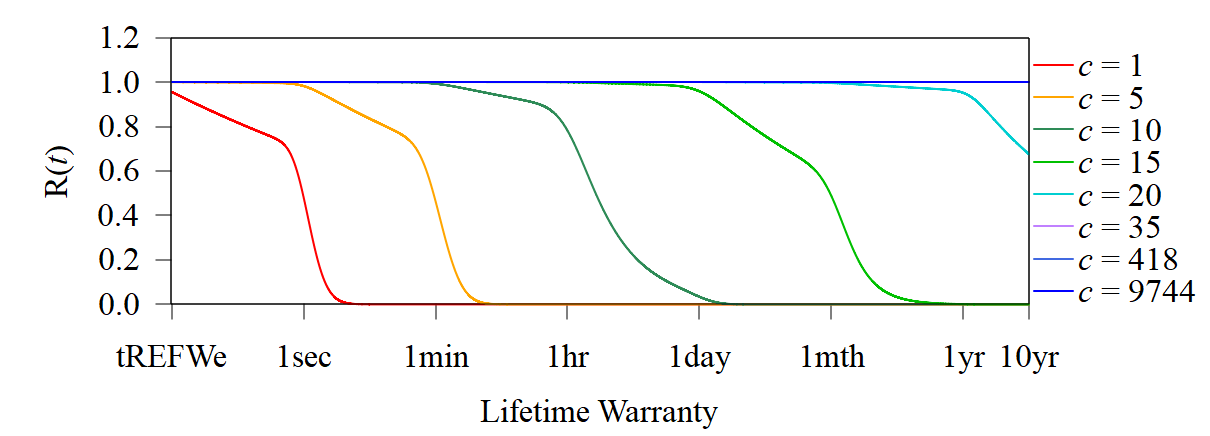
Figure 21: Example of Lifetime Warranty

Figure 21 displays DSAC’s lifetime warranty according to the number of counters. In the case of 20 counters, the required time of R(t) to be 0.999 is 9 days. This implies that DSAC can detect all the aggressor rows of double-sided uniform weight pattern for 9 days with 1,000 parts per million (ppm) error rate.

References

- [1] D. Anderson, P. Bevan, K. Lang, E. Liberty, L. Rhodes, and J. Thaler, “A High-Performance Algorithm for Identifying Frequent Items in Data Streams,” in Proceedings of the 2017 Internet Measurement Conference, 2017, pp. 268–282.
- [2] E. Bosman, K. Razavi, H. Bos, and C. Giuffrida, “Dedup Est Machina: Memory Deduplication as An Advanced Exploitation Vector,” in 2016 IEEE Symposium on Security and Privacy (S&P). IEEE, 2016, pp. 987–1004.
- [3] C. Callegari, S. Giordano, M. Pagano, and T. Pepe, “Detecting Heavy Change in The Heavy Hitter Distribution of Network Traffic,” in 2011 7th International Wireless Communications and Mobile Computing Conference. IEEE, 2011, pp. 1298–1303.
- [4] Y. Chen, G. Dong, J. Han, B. W. Wah, and J. Wang, “Multi-Dimensional Regression Analysis of Time-Series Data Streams,” in VLDB’02: Proceedings of the 28th International Conference on Very Large Databases. Elsevier, 2002, pp. 323–334.
- [5] L. Cojocar, K. Razavi, C. Giuffrida, and H. Bos, “Exploiting Correcting Codes: On The Effectiveness of ECC Memory against Rowhammer Attacks,” in 2019 IEEE Symposium on Security and Privacy (S&P). IEEE, 2019, pp. 55–71.
- [6] G. Cormode and M. Hadjieleftheriou, “Finding Frequent Items in Data Streams,” Proceedings of the VLDB Endowment, vol. 1, no. 2, pp. 1530–1541, 2008.
- [7] G. Cormode and M. Hadjieleftheriou, “Methods for Finding Frequent Items in Data Streams,” The VLDB Journal, vol. 19, no. 1, pp. 3–20, 2010.
- [8] G. Cormode and S. Muthukrishnan, “An Improved Data Stream Summary: The Count-min Sketch and Its Applications,” Journal of Algorithms, vol. 55, no. 1, pp. 58–75, 2005.
- [9] G. Cormode and S. Muthukrishnan, “What’s New: Finding Significant Differences in Network Data Streams,” IEEE/ACM Transactions on Networking, vol. 13, no. 6, pp. 1219–1232, 2005.
- [10] A. Das, “Hynix DRAM Layout, Process Integration Adapt to Change,” 2012.
- [11] P. Frigo, E. Vannacc, H. Hassan, V. Van Der Veen, O. Mutlu, C. Giuffrida, H. Bos, and K. Razavi, “TRRespass: Exploiting The Many Sides of Target Row Refresh,” in 2020 IEEE Symposium on Security and Privacy (S&P). IEEE, 2020, pp. 747–762.
- [12] C. Giannella, J. Han, J. Pei, X. Yan, and P. S. Yu, “Mining Frequent Patterns in Data Streams at Multiple Time Granularities,” Next generation data mining, vol. 212, pp. 191–212, 2003.
- [13] D. Gruss, M. Lipp, M. Schwarz, D. Genkin, J. Juffinger, S. O’Connell, W. Schoechl, and Y. Yarom, “Another Flip in The Wall of Rowhammer Defenses,” in 2018 IEEE Symposium on Security and Privacy (S&P). IEEE, 2018, pp. 245–261.
- [14] D. Gruss, C. Maurice, and S. Mangard, “Rowhammer. js: A Remote Software-Induced Fault Attack in JavaScript,” in International Conference on Detection of Intrusions and Malware, and Vulnerability Assessment. Springer, 2016, pp. 300–321.
- [15] N. Hua, B. Lin, J. Xu, and H. Zhao, “Brick: A Novel Exact Active Statistics Counter Architecture,” in Proceedings of the 4th ACM/IEEE Symposium on Architectures for Networking and Communications Systems, 2008, pp. 89–98.
- [16] JEDEC, “Double Data Rate 4 (DDR4) SDRAM Specification,” 2014.
- [17] JEDEC, “Low Power Double Data Rate 4 (LPDDR4) SDRAM Specification,” 2014.
- [18] JEDEC, “Low Power Double Data Rate 5 (LPDDR5) SDRAM Specification,” 2019.
- [19] JEDEC, “Double Data Rate 5 (DDR5) SDRAM Specification,” 2020.
- [20] JEDEC, “Graphics Double Data Rate 6 (GDDR6) SGRAM Specification,” 2021.
- [21] JEDEC, “High Bandwidth Memory (HBM) DRAM Specification,” 2021.
- [22] JEDEC, “JEP301-1: System Level Rowhammer Mitigation,” 2021.
- [23] S. Jeon, J. Choi, H.-c. Jung, S. Kim, and T. Lee, “Investigation on The Local Variation in BCAT Process for DRAM Technology,” in 2017 IEEE International Reliability Physics Symposium (IRPS). IEEE, 2017, pp. FA–4.
- [24] I. Kang, E. Lee, and J. H. Ahn, “CAT-TWO: Counter-Based Adaptive Tree, Time Window Optimized for DRAM Row-Hammer Prevention,” IEEE Access, vol. 8, pp. 17 366–17 377, 2020.
- [25] D.-H. Kim, P. J. Nair, and M. K. Qureshi, “Architectural Support for Mitigating Row Hammering in DRAM Memories,” IEEE Computer Architecture Letters, vol. 14, no. 1, pp. 9–12, 2014.
- [26] K. Kim, “Technology for Sub-50nm DRAM and NAND Flash Manufacturing,” in IEEE InternationalElectron Devices Meeting, 2005. IEDM Technical Digest. IEEE, 2005, pp. 323–326.
- [27] Y. Kim, R. Daly, J. Kim, C. Fallin, J. H. Lee, D. Lee, C. Wilkerson, K. Lai, and O. Mutlu, “Flipping Bits in Memory without Accessing Them: An Experimental Study of DRAM Disturbance Errors,” ACM SIGARCH Computer Architecture News, vol. 42, no. 3, pp. 361–372, 2014.
- [28] B. Krishnamurthy, S. Sen, Y. Zhang, and Y. Chen, “Sketch-based Change Detection: Methods, Evaluation, and Applications,” in Proceedings of the 3rd ACM SIGCOMM Conference on Internet Measurement, 2003, pp. 234–247.
- [29] A. Kurmus, N. Ioannou, M. Neugschwandtner, N. Papandreou, and T. Parnell, “From Random Block Corruption to Privilege Escalation: A Filesystem Attack Vector for Rowhammer-like Attacks,” in 11th USENIX Workshop on Offensive Technologies (WOOT) 17, 2017.
- [30] E. Lee, I. Kang, S. Lee, G. E. Suh, and J. H. Ahn, “TWiCe: Preventing Row-Hammering by Exploiting Time Window Counters,” in Proceedings of the 46th International Symposium on Computer Architecture, 2019, pp. 385–396.
- [31] Y. Lim and U. Kang, “Time-Weighted Counting for Recently Frequent Pattern Mining in Data Streams,” Knowledge and Information Systems, vol. 53, no. 2, pp. 391–422, 2017.
- [32] M. Lipp, M. Schwarz, L. Raab, L. Lamster, M. T. Aga, C. Maurice, and D. Gruss, “Nethammer: Inducing Rowhammer Faults through Network Requests,” in 2020 IEEE European Symposium on Security and Privacy Workshops (EuroS&PW). IEEE, 2020, pp. 710–719.
- [33] Y. Liu, “Data Streaming Algorithms for Rapid Cyber Attack Detection,” 2013.
- [34] N. Manerikar and T. Palpanas, “Frequent Items in Streaming Data: An Experimental Evaluation of The State-of-the-art,” Data & Knowledge Engineering, vol. 68, no. 4, pp. 415–430, 2009.
- [35] G. S. Manku and R. Motwani, “Approximate Frequency Counts Over Data Streams,” in VLDB’02: Proceedings of the 28th International Conference on Very Large Databases. Elsevier, 2002, pp. 346–357.
- [36] A. Metwally, D. Agrawal, and A. E. Abbadi, “An Integrated Efficient Solution for Computing Frequent and Top-k Elements in Data Streams,” ACM Transactions on Database Systems (TODS), vol. 31, no. 3, pp. 1095–1133, 2006.
- [37] J. Misra and D. Gries, “Finding Repeated Elements,” Science of Computer Programming, vol. 2, no. 2, pp. 143–152, 1982.
- [38] N. Muralimanohar, R. Balasubramonian, and N. P. Jouppi, “CACTI 6.0: A Tool to Model Large Caches,” HP laboratories, vol. 27, p. 28, 2009.
- [39] S.-W. Park, S.-J. Hong, J.-W. Kim, J.-G. Jeong, K.-D. Yoo, S.-C. Moon, H.-C. Sohn, N.-J. Kwak, Y.-S. Cho, S.-J. Baek, H.-S. Park, H. G. Yoon, B.-H. Lee, J.-S. Kim, S.-H. Hwang, L.-H. Lee, H.-J. Cho, S. Y. Cho, C.-O. Chung, K.-O. Kim, M.-S. Yoo, S.-A. Jang, S.-D. Lee, and S.-W. Chung, “Highly Scalable Saddle-Fin (S-Fin) Transistor for Sub-50nm DRAM Technology,” in 2006 Symposium on VLSI Technology, 2006. Digest of Technical Papers. IEEE, 2006, pp. 32–33.
- [40] Y. Park, W. Kwon, E. Lee, T. J. Ham, J. H. Ahn, and J. W. Lee, “Graphene: Strong yet Lightweight Row hammer Protection,” in 2020 53rd Annual IEEE/ACM International Symposium on Microarchitecture (MICRO). IEEE, 2020, pp. 1–13.
- [41] M. K. Qureshi, A. Jaleel, Y. N. Patt, S. C. Steely, and J. Emer, “Adaptive Insertion Policies for High Performance Caching,” ACM SIGARCH Computer Architecture News, vol. 35, no. 2, pp. 381–391, 2007.
- [42] K. Razavi, B. Gras, E. Bosman, B. Preneel, C. Giuffrida, and H. Bos, “Flip Feng Shui: Hammering A Needle in The Software Stack,” in 25th USENIX Security Symposium USENIX Security 16, 2016, pp. 1–18.
- [43] T. Schloesser, F. Jakubowski, J. v. Kluge, A. Graham, S. Slesazeck, M. Popp, P. Baars, K. Muemmler, P. Moll, K. Wilson, A. Buerke, D. Koehler, J. Radecker, E. Erben, U. Zimmermann, T. Vorrath, B. Fischer, G. Aichmayr, R. Agaiby, W. Pamler, T. Schuster, W. Bergner, and W. Mueller, “6F2 Buried Wordline DRAM Cell for 40nm and Beyond,” in 2008 IEEE International Electron Devices Meeting. IEEE, 2008, pp. 1–4.
- [44] R. Schweller, Y. Chen, E. Parsons, A. Gupta, G. Memik, and Y. Zhang, “Reverse Hashing for Sketch-Based Change Detection on High-Speed Networks,” in Proceedings of ACM/USENIX Internet Measurement Conference’04, 2004.
- [45] M. Seaborn and T. Dullien, “Exploiting The DRAM Rowhammer Bug to Gain Kernel Privileges,” Black Hat, vol. 15, p. 71, 2015.
- [46] S. M. Seyedzadeh, A. K. Jones, and R. Melhem, “Counter-Based Tree Structure for Row Hammering Mitigation in DRAM,” IEEE Computer Architecture Letters, vol. 16, no. 1, pp. 18–21, 2016.
- [47] M. Son, H. Park, J. Ahn, and S. Yoo, “Making DRAM Stronger against Row Hammering,” in Proceedings of the 54th Annual Design Automation Conference 2017, 2017, pp. 1–6.
- [48] A. Tatar, R. K. Konoth, E. Athanasopoulos, C. Giuffrida, H. Bos, and K. Razavi, “Throwhammer: Rowhammer Attacks over The Network and Defenses,” in 2018 USENIX Annual Technical Conference (ATC) 18, 2018, pp. 213–226.
- [49] M. Technology, “Micron Product Lifecycle Solutions,” 2018.
- [50] D. Tong and V. Prasanna, “High Throughput Sketch Based Online Heavy Change Detection on FPGA,” in 2015 International Conference on ReConFigurable Computing and FPGAs (ReConFig). IEEE, 2015, pp. 1–8.
- [51] V. Van Der Veen, Y. Fratantonio, M. Lindorfer, D. Gruss, C. Maurice, G. Vigna, H. Bos, K. Razavi, and C. Giuffrida, “Drammer: Deterministic Rowhammer Attacks on Mobile Platforms,” in Proceedings of the 2016 ACM SIGSAC Conference on Computer and Communications Security, 2016, pp. 1675–1689.
- [52] V. Van der Veen, M. Lindorfer, Y. Fratantonio, H. P. Pillai, G. Vigna, C. Kruegel, H. Bos, and K. Razavi, “GuardION: Practical Mitigation of DMA-based Rowhammer Attacks on ARM,” in International Conference on Detection of Intrusions and Malware, and Vulnerability Assessment. Springer, 2018, pp. 92–113.
- [53] A. J. Walker, S. Lee, and D. Beery, “On DRAM Rowhammer and The Physics of Insecurity,” IEEE Transactions on Electron Devices, vol. 68, no. 4, pp. 1400–1410, 2021.
- [54] WikiChip, “Intel Cascade Lake SP.”
- [55] Y. Xiao, X. Zhang, Y. Zhang, and R. Teodorescu, “One Bit Flips, One Cloud Flops: Cross-VM Row Hammer Attacks and Privilege Escalation,” in 25th USENIX Security Symposium USENIX Security 16, 2016, pp. 19–35.
- [56] A. G. Yağlıkçı, M. Patel, J. S. Kim, R. Azizi, A. Olgun, L. Orosa, H. Hassan, J. Park, K. Kanellopoulos, T. Shahroodi, S. Ghose, and O. Mutlu, “BlockHammer: Preventing RowHammer at Low Cost by Blacklisting Rapidly-Accessed DRAM Rows,” arXiv preprint arXiv:2102.05981, 2021.
- [57] C.-M. Yang, C.-K. Wei, Y. J. Chang, T.-C. Wu, H.-P. Chen, and C.-S. Lai, “Suppression of Row Hammer Effect by Doping Profile Modification in Saddle-fin Array Devices for Sub-30-nm DRAM Technology,” IEEE Transactions on Device and Materials Reliability, vol. 16, no. 4, pp. 685–687, 2016.
- [58] M. S. Yoo, K. S. Choi, and W. K. Sun, “Saddle-fin Cell Transistors with Oxide Etch Rate Control by Using Tilted Ion Implantation (TIS-Fin) for Sub-50-nm DRAMs,” Journal of the Korean Physical Society, vol. 56, no. 2, pp. 643–647, 2010.
- [59] J. M. You and J.-S. Yang, “MRLoc: Mitigating Row-Hammering Based on Memory Locality,” in 2019 56th ACM/IEEE Design Automation Conference (DAC). IEEE, 2019, pp. 1–6.
- [60] M. Zadnik and M. Canini, “Evolution of Cache Replacement Policies to Track [h]eavy-hitter Flows,” in International Conference on Passive and Active Network Measurement. Springer, 2011, pp. 21–31.
- [61] T. Zhang, K. Chen, C. Xu, G. Sun, T. Wang, and Y. Xie, “Half-DRAM: A High-bandwidth and Low-power DRAM Architecture from The Rethinking of Fine-grained Activation,” in 2014 ACM/IEEE 41st International Symposium on Computer Architecture (ISCA). IEEE, 2014, pp. 349–360.