Strictly Frequentist Imprecise Probability
Abstract
Strict frequentism defines probability as the limiting relative frequency in an infinite sequence. What if the limit does not exist? We present a broader theory, which is applicable also to random phenomena that exhibit diverging relative frequencies. In doing so, we develop a close connection with the theory of imprecise probability: the cluster points of relative frequencies yield a coherent upper prevision. We show that a natural frequentist definition of conditional probability recovers the generalized Bayes rule. This also suggests an independence concept, which is related to epistemic irrelevance in the imprecise probability literature. Finally, we prove constructively that, for a finite set of elementary events, there exists a sequence for which the cluster points of relative frequencies coincide with a prespecified set which demonstrates the naturalness, and arguably completeness, of our theory.
1 Introduction
Do other statistical properties, that can not be reduced
to stochasticness, exist? This question did not attract
any attention until the applications of the probability
theory concerned only natural sciences. The situation is
definitely [changing], when one studies social phenomena:
the stochasticness gets broken as soon as we [deal] with
deliberate activity of people.
— Victor Ivanenko and Valery Labkovsky (1993)
It is now almost universally acknowledged that probability theory ought to be based on Kolmogorov’s (1933) mathematical axiomatization (translated in (Kolmogorov, 1956)).111An important exception is quantum probability (Gudder, 1979; Khrennikov, 2016). However, if probability is defined in this purely measure-theoretic fashion, what warrants its application to real-world problems of decision making under uncertainty? To those in the so-called frequentist camp, the justification is essentially due to the law of large numbers, which comes in both an empirical and a theoretical flavour. Our motivation for the present paper comes from questioning both of these.
By the empirical version of the law of large numbers (LLN), we mean not a “law” which can be proven to hold, but the following hypothesis, which seems to guide many scientific endeavours. Assume we have obtained data as the outcomes of some experiment, which has been performed times under “statistically identical” conditions. Of course, conditions in the real-world can never truly be identical — otherwise the outcomes would be constant, at least under the assumption of a deterministic universe. Thus, “identical” in this context must be a weaker notion, that all factors which we have judged as relevant to the problem at hand have been kept constant over the repetitions.222In fact, we do not need that conditions stay exactly constant, but that they change merely in a way which is so benign that the relative frequencies converge. That is, in the limit we should obtain a stable statistical aggregate. The empirical “law” of large numbers, which Gorban (2017) calls the hypothesis of (perfect) statistical stability then asserts that in the long-run, relative frequencies of events and sample averages converge. These limits are then conceived of as the probability of an event and the expectation, respectively. Thus, even if relative frequencies can fluctuate in the finite data setting, we expect that they stabilize as more and more data is acquired. Crucially, this hypothesis of perfect statistical stability is not amenable to falsification, since we can never refute it in the finite data setting. It is a matter of faith to assume convergence of relative frequencies. On the other hand, there is now ample experimental evidence that relative frequencies can fail to stabilize even under very long observation intervals (Gorban, 2017, Part II). We say that such phenomena display unstable (diverging) relative frequencies. Rather than refuting the stability hypothesis, which is impossible, we question its adequateness as an idealized modeling assumption: we view convergence as the idealization of approximate stability in the finite case, whereas divergence idealizes instability. Thus, if probability is understood as limiting relative frequency, then the applicability of Kolmogorov’s theory to empirical phenomena is limited to those which are statistically stable; the founder himself remarked:
Generally speaking there is no ground to believe that a random phenomenon should possess any definite probability (Kolmogorov, 1983).
Building on the works of von Mises & Geiringer (1964), Walley & Fine (1982) and Ivanenko (2010), our goal is to establish a broader theory, which is also applicable to “random” phenomena which are outside of the scope of Kolmogorov’s theory by exhibiting unstable relative frequencies.
One attempt to “prove” (or justify) the empirical law of large numbers, which in our view is doomed to fail, is to invoke the theoretical law of large numbers, which is a purely formal, mathematical statement. The strong law of large numbers states that if is a sequence of independent and identically distributed (i.i.d.) random variables with finite expectation , then the sample average converges almost surely to the expectation:
where is the underlying probability measure in the sense of Kolmogorov. To interpret this statement correctly, some care is needed. It asserts that assigns measure to the set of sequences for which the sample mean converges, but not that this happens for all sequences. Thus one would need justification for identifying “set of measure 0“ with “is negligible” (“certainly does not happen”), which in particular requires a justification for . With respect to a different measure, this set might not be negligible at all (Schnorr, 2007, p. 8); see also (Calude & Zamfirescu, 1999; Seidenfeld et al., 2017) for critical arguments. Moreover, the examples in (Gorban, 2017, Part II) show that sequences with seemingly non-converging relative frequencies (fluctuating substantially even for long observation intervals) are not “rare” in practice. In Appendix E we examine the question of how pathological or normal such sequences are in more depth.
Conceptually, the underlying problem is that the probability measure , which is used to measure the event has no clear meaning. Of course, in the subjectivist spirit, one could interpret it as assigning a belief in the statement that convergence takes place. But it is unclear what a frequentist interpretation of would look like. As La Caze (2016) observed:
Importantly, “almost sure convergence” is also given a frequentist interpretation. Almost sure convergence is taken to provide a justification for assuming that the relative frequency of an attribute would converge to the probability in actual experiments were the experiment to be repeated indefinitely [emphasis in original].
But again, it is unclear on what ground can be given this interpretation and according to Hájek (2009) this leads to a regress to mysterious “meta-probabilities”. Furthermore, the theoretical LLN requires that be countably additive, which is problematic under a frequency interpretation (Hájek, 2009, pp. 229–230).
Given these complications, we opt for a different approach, namely a strictly frequentist one. Reaching back to Richard von Mises’ (1919) foundational work, a strictly frequentist theory explicitly defines probability in terms of limiting relative frequencies in a sequence. Importantly, we here do not assume that the elements of the sequence are random variables with respect to an abstract, countably additive probability measure. Instead, like von Mises, we actually take the notion of a sequence as the primitive entity in the theory. As a consequence, countable additivity does not naturally arise in this setting, and hence we do not subscribe to the frequentist interpretation of the classical strong LLN.
The core motivation for our work is to drop the assumption of perfect statistical stability and instead to explicitly model the possibility of unstable (diverging) relative frequencies. Rather than merely conceding that the “probability” might vary over time (Borel, 1963, pp. 27ff.) (which begs the question what such “probabilities” mean) we follow the approach of Ivanenko (2010), reformulate his construction of a statistical regularity of a sequence, and discover that it is closely connected to the subjectivist theory of imprecise probability. In essence, to each sequence we can naturally associate a set of probability measures, which constitute the statistical regularity that describes the cluster points of relative frequencies and consequently also those of sample averages. Since this works for any sequence and any event, we have thus countered a typical argument against frequentism, namely that the limit may not exist and hence probability is undefined (Hájek, 2009). The relative frequencies induce a coherent upper probability and the sample averages induce a coherent upper prevision in the sense of Walley (1991). In the convergent case, this reduces to a precise, finitely additive probability and a linear prevision, respectively. Furthermore, we derive in a natural way a conditional upper prevision; remarkably, this approach recovers the generalized Bayes rule, the arguably most important updating principle in imprecise probability.
Furthermore, we demonstrate that the reverse direction works, too: given a set of probability measures, we can explicitly construct a sequence, which corresponds to this set in the sense that its relative frequencies have this set of cluster points. Thereby we establish strictly frequentist semantics for imprecise probability: a subjective decision maker who uses a set of probability measures to represent their belief can also be understood as assuming an implicit underlying sequence and reasoning in a frequentist way thereon.
1.1 Von Mises - The Frequentist Perspective
Our approach is inspired by Richard von Mises (1919) (refined and summarized in (von Mises & Geiringer, 1964)) axiomatization of probability theory. In contrast to the subjectivist camp, von Mises concern was to develop a theory for repetitive events; which gives rise to a theory of probability that is mathematical, but which can also be used to reason about the physical world.
The calculus of probability, i.e. the theory of probabilities, in so far as they are numerically representable, is the theory of definite observable phenomena, repetitive or mass events. Examples are found in games of chance, population statistics, Brownian motion etc. (von Mises, 1981, p. 102).
Hence, von Mises is not concerned with the probability of single events, which he deems meaningless, but instead always views an event as part of a larger reference class. Such a reference class is captured by what he terms a collective, a disorderly sequence which exhibits both global regularity and local irregularity.
Definition 1.1.
Consider a tuple with the following data:
-
1.
a sequence ;
-
2.
a set of selection rules , where for each in a countable index set , and for infinitely many ;
-
3.
a non-empty set system , where for simplicity we assume .333In fact, does not necessarily has to be finite. Since an infinite domain of probabilities does not contribute a lot to a better understanding of the frequentist definition at this point, we restrict ourselves to the finite case here. The reader can find details in (von Mises & Geiringer, 1964).
This tuple forms a collective if the following two axioms hold.
-
vM1.
The limiting relative frequency for exists:
We call this limit the probability of .
-
vM2.
For each , the selection rule does not change limiting relative frequencies:555To be precise, a selection rule in the sense of von Mises is a map from the set of finite -valued strings to , i.e. a selection rule is able to “see” all previous elements when deciding whether or not to select the next one. Our formulation is more restrictive to avoid notational overhead, but when a sequence is fixed, the two formulations are equivalent.
Here, we view as a sequence of elementary outcomes , for some possibility space on which we have a set system of events . Axiom vM1 explicitly defines the probability of an event in terms of the limit of its relative frequency. Demanding that this limit exists is non-trivial, since this need not be the case for an arbitrary sequence. Intuitively, vM1 expresses the hypothesis of statistical stability, which captures a global regularity of the sequence.
In contrast, vM2 captures a sense of randomness or local irregularity. Note it actually comprises two claims: 1) the limit exists and 2) it is the same as the limit in vM1. It is best understood by viewing a selection rule as selecting a subsequence of the original sequence and then demanding that the limiting relative frequencies thereof coincide with those of the original sequence. Such a selection rule is called admissible, whereas a selection rule which would give rise to different limiting relative frequencies for at least one would be inadmissible. Why do we need axiom vM2? Von Mises calls this the “law of the excluded gambling system” and it is the key to capture the notion of randomness in his framework. Intuitively, if a selection rule is inadmissible, an adversary could use this knowledge to strategically offer a bet on the next outcome and thereby make long-run profit, at the expense of our fictional decision maker. A random sequence, however, is one for which there does not exist such a betting strategy. It turns out, that this statement cannot hold in its totality. A sequence cannot be random with respect to all selection rules except in trivial cases (cf. Kamke’s critique of von Mises’ notion of randomness, nicely summarized in (van Lambalgen, 1987)). Thus, von Mises explicitly relativizes randomness with respect to a problem-specific set of selection rules (von Mises & Geiringer, 1964, p. 12).666This class of selection rules necessarily must be specified in advance; confer (Shen, 2009). A prominent line of work aspires to fix the set of selection rules as all partially computable selection rules (Church, 1940), but there is no compelling reason to elevate this to a universal choice; cf. (Derr & Williamson, 2022) for an elaborated critique. A sequence which forms a collective (“is random with respect to”) one set of selection rules, might not form a collective with respect to another set.
In our view, the role of the randomness axiom vM2 is similar to the role of more familiar randomness assumptions like the standard i.i.d. assumption: to empower inference from finite data. In this work, however, we will be exclusively concerned with the idealized case of infinite data, since our focus is the axiom (or hypothesis) of statistical stability.
We are motivated by the following question. What happens to von Mises approach when axiom vM1 breaks down? That is, when relative frequencies of at least some events do not converge. Our answer leads to a confluence with a theory that is thoroughly grounded in the subjectivist camp: the theory of imprecise probability. In summary, we establish a strictly frequentist theory of imprecise probability.
1.2 Imprecise Probability - The Subjectivist Perspective
We briefly introduce the prima facie unrelated, subjectivist theory of imprecise probability, or more specifically, the theory of lower and upper previsions as put forward by Walley (1991). Orthodox Bayesianism models belief via the assignment of precise probabilities to propositions, or equivalently, via a linear expectation functional. In contrast, in Walley’s theory, belief is interval-valued and the linear expectation is replaced by a pair of a lower and upper expectation. Hence, the theory is strictly more expressive than orthodox Bayesianism, which can be recovered as a special case.
We assume an underlying possibility set , where is an elementary event, which includes all relevant information. We call a function , which is bounded, i.e. , a gamble and collect all such functions in the set . The set of gambles carries a vector space structure with scalar multiplication , , and addition . For a constant gamble we write simply . Note that Walley’s theory in the general case does not require that a vector space of gambles is given, but definitions and results simplify significantly in this case.
We interpret a gamble as assigning an uncertain loss to each elementary event, that is, in line with the convention in insurance and machine learning, we take positive values to represent loss and negative values to represent reward.777Unfortunately, this introduces tedious sign flips when comparing results to Walley (1991). We imagine a decision maker who is faced with the question of how to value a gamble ; the orthodox answer would be the expectation with respect to a subjective probability measure.
Walley (1991) proposed a betting interpretation of imprecise probability, which is inspired by de Finetti (1974/2017), who identifies probability with fair betting rates. The goal is to axiomatize a functional , which assigns to a gamble the smallest number so that is a desirable transaction to our decision maker, where she incurs the loss but in exchange gets the reward . Formally:
where is a set of desirable gambles. Walley (1991, Section 2.5) argued for a criterion of coherence, which any reasonable functional should satisfy, and consequently obtained the following characterization (Walley, 1991, Theorem 2.5.5), which we shall take here as an axiomatic definition instead.888Here, we need the vector space assumption on the set of gambles. We also note that Walley (1991, pp. 64–65) himself made a similar definition, but then proposed the more general coherence concept.
Definition 1.2.
A functional is a coherent upper prevision if it satisfies :
-
UP1.
(bounds)
-
UP2.
(positive homogeneity)
-
UP3.
(subadditivity)
Together, these properties also imply (Walley, 1991, p. 76):
-
UP4.
(translation equivariance)
-
UP5.
(monotonicity)
To a coherent upper prevision, we can define its conjugate lower prevision by:
which specifies the highest certain loss that the decision maker is willing to shoulder in exchange for giving away the loss , i.e. receiving the reward . Due to the conjugacy, it suffices to focus on the upper prevision throughout. In general, we have that for any . If , we say that is a linear prevision, a definition which aligns with de Finetti (1974/2017).
By applying an upper prevision to indicator gambles, we obtain an upper probability , where . Correspondingly, the lower probability is . In the precise case, there is a unique relationship between (finitely) additive probabilities and linear previsions; however, upper previsions are more expressive than upper probabilities. Finally, we remark that via the so-called natural extension, a coherent upper probability which is defined on some subsets of events can be extended to a coherent upper prevision on , which is compatible with in the sense that (cf. (Walley, 1991, Section 3.1)).
2 Unstable Relative Frequencies
Assume that we have some fixed sequence on a possibility set of elementary events, but that for some events , where , the limiting relative frequencies do not exist. What can we do then? In a series of papers (Ivanenko & Labkovskii, 1986a; b; 1990; 1993; Ivanenko & Munier, 2000; Ivanenko & Labkovskii, 2015; Ivanenko & Pasichnichenko, 2017) and a monograph (Ivanenko, 2010), Ivanenko and collaborators have developed a strictly frequentist theory of “hyper-random phenomena” based on “statistical regularities”. In essence, they tackle mass decision making in the context of sequences with possibly divergent relative frequencies. Like von Mises, they take the notion of a sequence as the primitive, that is, without assuming an a priori probability and then invoking the law of large numbers. They explicitly recognize that “stochasticness gets broken as soon as we deal with deliberate activity of people” (Ivanenko & Labkovskii, 1993)999This not only occurs because of non-equilibrium effects, but also from feedback loops, what has become known as “performativity” (MacKenzie et al., 2007) or “reflexivity” (Soros, 2009). See the epigraph at the beginning of the present paper.. The presentation of Ivanenko’s theory is obscured somewhat by the great generality with which it is presented (they work with general nets, rather than just sequences). We build heavily upon their work but entirely restrict ourselves to working with sequences. While in some sense this is a weakening, our converse result (see Section 3 is actually stronger as we show that one can achieve any “statistical regularity” by taking relative frequencies of only sequences. For simplicity, we will dispense with integrals with respect to finitely additive measures in our presentation, so that there are less mathematical dependencies involved;101010The two well-known accounts of the theory of integrals with finitely additive measures are (Rao & Rao, 1983) and (Dunford & Schwartz, 1988). The theory of linear previsions as laid out in (Walley, 1991) appears to be an easier approach for our purposes. instead, we work with linear previsions. Moreover, we establish111111Ivanenko & Labkovskii (2015) mention in passing that sets of probabilities also appear in (Walley, 1991). the connection to imprecise probability and give a different justification for the construction.
2.1 Ivanenko’s Argument — Informally
We begin by providing an informal summary of Ivanenko’s construction of statistical regularities on sequences. Assume we are given a fixed sequence of elementary events , where we may intuitively think of as representing time. In contrast to von Mises, who demands the existence of relative frequency limits to define probabilities, we ask for something like a probability for all events , even when the relative frequencies have no limit. To this end, we exploit that sequences of relative frequencies always have a non-empty set of cluster points, each of which is a finitely additive probability. Hence, a decision maker can use this set of probabilities to represent the global statistical properties of the sequence. In fact, we will see that this induces a coherent upper probability. Also, our decision maker is interested in assessing a value for each gamble , which is evaluated infinitely often over time. Here, the sequence of averages is the object of interest. In the case of convergent relative frequencies, a decision maker would use the expectation to assess the risk in the limit, whereas in the general case of possible non-convergence, a different object is needed. This object turns out to be a coherent upper prevision. We provide a justification for using this upper prevision to assess the value of a gamble, which links it to imprecise probability.
2.2 Ivanenko’s Argument — Formally
Let be an arbitrary (finite, countably infinite or uncountably infinite) set of outcomes and fix , an -valued sequence. We define a gamble as a bounded function from to , i.e. and collect all such gambles in the set . We assume the vector space structure on as in Section 1.2.
The set becomes a Banach space, i.e. a complete normed vector space, under the supremum norm . We denote the topological dual space of by . Recall that it consists exactly of the continuous linear functionals . We endow with the weak*-topology, which is the weakest topology (i.e. with the fewest open sets) that makes all evaluation functionals of the form , for any and continuous. Consider the following subset of :
Due to the Alaoglu-Bourbaki theorem, this set is compact under the weak* topology, see Appendix A.1.
A finitely additive probability on some set system , where , is a function such that:
-
PF1.
.
-
PF2.
whenever and .
We induce a sequence of finitely additive probabilities where for each . It is easy to check that indeed is a finitely additive probability on the whole powerset for any . We shall call the sequence of empirical probabilities. Due to (Walley, 1991, Corollary 3.2.3), a finitely additive probability defined on can be uniquely extended (via natural extension) to a linear prevision , so that . Furthermore, we know from (Walley, 1991, Corollary 2.8.5), that there is a one-to-one correspondence between elements of and linear previsions . Hence, we associate to each empirical probability an empirical linear prevision , where and we denote the natural extension by . We thus obtain a sequence .
On the other hand, each gamble induces a sequence of evaluations as , where . For , we define the sequence of averages of the gamble over time as , where . For each finite , we can also view the average as a function in , i.e. . Observe that this is a coherent linear prevision and by applying it to indicator gambles , we obtain . Hence, we know from (Walley, 1991, Corollary 3.2.3) that this linear prevision is in fact the natural extension of , i.e. . This concludes the technical setup; we now begin reproducing Ivanenko’s argument.
Since is a compact topological space under the subspace topology induced by the weak*-topology on , we know that any sequence has a non-empty closed set of cluster points. Recall that a point is a cluster point of a sequence , where is any topological space, if:
We remark that this does not imply that those cluster points are limits of convergent subsequences.121212This would hold under sequential compactness, which is not fulfilled here in general, but it is for finite . We denote the set of cluster points as . Equivalently, by applying these linear previsions to indicator gambles, we obtain the set of finitely additive probabilities . Due to the one-to-one relationship, we might work with either or . Following Ivanenko, we call the statistical regularity of the sequence ; in the language of imprecise probability, it is a credal set.
We further define
where , and
Observe that is defined on all and is defined on all subsets of , even if is uncountably infinite, since each is a finitely additive probability on . We further observe that is a coherent upper prevision on or equivalently, a coherent risk measure in the sense of Artzner et al. (1999).131313For the close connection of coherent upper previsions and coherent risk measures we refer to (Fröhlich & Williamson, 2022). Correspondingly, is a coherent upper probability on , which is obtained by applying to indicator functions. This follows directly from the envelope theorem in (Walley, 1991, Theorem 3.3.3).
So far, the definition of and may seem unmotivated. Yet they play a special role, as we now show.
Proposition 2.1.
The sequence of averages has the set of cluster points
and therefore
Proof.
First observe that
We use the following result from (Ivanenko & Pasichnichenko, 2017, Lemma 3).141414A subtle point in the argument, which Ivanenko & Pasichnichenko (2017) do not make visible, is the sequential compactness of , which means that for any cluster point of an -valued sequence we can find a subsequence converging to it.
Lemma 2.2.
Let be a continuous function on a compact space and a -valued sequence. Then .
On the right side, the application of is to be understood as applying to each element in the set . Consider now the evaluation functional , , which is continuous under the weak*-topology. The application of the lemma with , , hence gives:
But since , we obtain that . ∎
A similar statement holds for the coherent upper probability.
Corollary 2.3.
For any , .
Proof.
Just observe that and apply the previous result. ∎
Thus the limes superior of the sequence of relative frequencies induces a coherent upper probability on ; similarly, the limes superior of the sequence of a gamble’s averages induces a coherent upper prevision on . By conjugacy, we have that the lower prevision and lower probability are :
which are obtained in a similar way using the limes inferior. Finally, when an event is precise in the sense that (and thus the equals the and hence the limit exists), we denote the upper (lower) probability as and say that the precise probability of exists.
2.3 The Induced Upper Prevision
We have seen that the upper prevision , as we have just defined it, has the property that it is induced by the statistical regularity of the sequence, and at the same time corresponds to taking the supremum over the cluster points of the sequence of averages of a gamble over time. The set of cluster points is in general a complicated object, hence it is unclear why one should take the supremum to reduce it to a single number in a decision making context. Our goal in this section is to provide some intuition why it is reasonable to use , as we defined it, to assess the risk inherent in a sequence. Ivanenko & Munier (2000) argued that is the unique object which satisfies a certain list of axioms, which are similar to those for an upper prevision, but including a so-called “principle of guaranteed result”, which appears rather mysterious to us.
Our setup is as follows. We imagine an individual decision maker, who is faced with a fixed sequence and various gambles . The question to the decision maker is how to value this gamble in light of the sequence, i.e. imagining that the gamble is evaluated at each , infinitely often. Here, represents a loss for positive values, and a gain for negative values. We can think of the as the states of nature, and the sequence determines which are realized and how often. Importantly, we view our decision maker as facing a mass decision, i.e. the gamble will not only be evaluated once, but instead infinitely often.
Which gambles are desirable to our decision maker? Desirable gambles151515We remark that throughout the paper we always mean almost desirability, cf. (Walley, 1991, Section 3.7). are those which the decision maker would accept even without any reward for it. We argue that an appropriate set of desirable gambles is given by:
Consider what means. If the limes superior of the gamble’s average sequence, i.e. the growth rate of the accumulated loss, is negative or zero, then we are guaranteed that there is no strictly positive accumulated loss which we will face infinitely often. The choice of the average as the aggregation functional is justified from the mass decision character of the setting, since we assume that our decision maker does not care about individual outcomes, but only about long-run capital. Now, given this set of desirable gambles, we seek a functional , so that when at each time step , the transaction takes place, this results in a desirable gamble for our decision maker. Our decision maker shoulders the loss , while at the same time asking for in advance. Intuitively, is supposed to be the certainty equivalent of the “uncertain” loss , in the sense that will vary over time. Therefore we define, in correspondence with , the upper and lower previsions ():
| (1) | ||||
When a set of desirable gambles and an upper (lower) prevision are in this correspondence, it holds that and furthermore is the least (smallest) functional for which this holds. We can now observe that in fact , since
is the general correspondence for a set of desirable gambles and a coherent upper prevision. Hence, we have motivated the definition of in Section 2.2. It is easy to see explicitly (cf. Appendix A.2) that and that is in fact the smallest number such that the relation in Equation 1 holds.
3 From Cluster Points to Sequence
In the previous section, we have shown how from a given sequence we can construct a coherent upper prevision from the set of cluster points . In this section, we show the converse, thus “closing the loop”: given an arbitrary coherent upper prevision, we construct a sequence such that the induced upper prevision is just the specified one. We take this to be an argument for the well-groundedness of our approach. For simplicity, we assume a finite possibility space .
Theorem 3.1.
Let . Let be a coherent upper prevision on . There exists a sequence such that we can write as:
where we now make the dependence on the sequence explicit in the notation, i.e. .
The significance of this result is that it establishes strictly frequentist semantics for imprecise probability. It shows that to any decision maker who, in the subjectivist fashion, uses a coherent upper prevision, we can associate a sequence, which would yield the same upper prevision in a strictly frequentist way. We interpret this result as evidence for the naturalness, and arguably completeness, of our theory.
The key to prove this is Theorem 3.3, for which we introduce some convenient notation. For , let and define the -simplex as
It is also helpful to have a dual notation for sequences , whereby we write either or to mean the same thing.
Definition 3.2.
Suppose and . For any define the relative frequency of with respect to at , via
and the relative frequency of at , as
| (2) |
Theorem 3.3.
Suppose and is a rectifiable closed curve in . There exists such that .
The proof (which is constructive) is in Appendix C along with an example. From this, we obtain the following Corollary (proven in Appendix C.10). Denote the topological boundary of a set as .
Corollary 3.4.
Suppose and is a non-empty convex set. There exists such that .
Since we have a finite possibility space , we can identify each linear prevision with a point in the simplex, by assigning coordinates to its underlying finitely additive probability; in the case of , this is the relative frequency . This is formalized in the following.
Proposition 3.5.
Let be a sequence of linear previsions with underlying probabilities . Then with respect to the weak* topology if and only if the sequence , has as cluster point with respect to the topology induced by the Euclidean norm on .
For the proof, see Appendix C.1. Combining Corollary 3.4 and Proposition 3.5 allows us to now prove Theorem 3.1.
Proof of Theorem 3.1.
Let . If is a coherent upper prevision on , we can write it as (Walley, 1991, Theorem 3.6.1):
for some weak* compact and convex set . From (Walley, 1991, Theorem 3.6.2) we further know that
where denotes the set of extreme points of .161616A point is an extreme point of if it cannot be written as a convex combination of any other elements in . Then:
since and ; note that is closed. In summary, .
Ivanenko (2010) offers a somewhat similar result to Theorem 3.1 by generalizing from sequences to sampling nets. Ivanenko’s (2010) main result states that “any sampling directedness has a regularity, and any regularity is the regularity of some sampling directedness.” (Ivanenko, 2010, Theorem 4.2). We provide a brief introduction to Ivanenko’s setup in Appendix D. Our result is more parsimonious in the sense that it relies only on sequences, which are arguably more intuitive objects than such sampling nets.
Our result should also be compared to Theorem 4.2 in (Walley & Fine, 1982) and Theorem 2.2 in (Papamarcou & Fine, 1991b). On the one hand, our result is stronger since it holds for upper previsions, whereas Theorem 4.2 in (Walley & Fine, 1982) and Theorem 2.2 in (Papamarcou & Fine, 1991b) hold for upper probabilities only; note that upper previsions are more expressive than upper probabilities.171717Indeed, the proof of Theorem 4.2 in (Walley & Fine, 1982) exploits this simplification by assuming that the credal set has a finite number of extreme points. On the other hand, Theorem 2.2 in (Papamarcou & Fine, 1991b) is stronger in the sense that it guarantees that the same upper probability is induced when applying selection rules.
We observe that two sequences , , might have different sets of cluster points , , but when their convex hull coincides, the same upper probability and prevision is induced.181818Assume . Then indeed , where denotes the weak* closure of the convex hull; cf. (Walley, 1991, Section 3.6). Thus, in light of the argument in Section 2.3, for the purpose of mass decision making, we may consider these sequences equivalent. While in the classical case, relative frequencies are the relevant description of a sequence, the statistical regularity provides an analogous description in the general case; moreover, we differentiate only “up to the same convex hull” for decision making.
4 Unstable Conditional Probability
An interesting aspect of the strictly frequentist approach is that there is a natural way of introducing conditional probability for events , which is the same for the case of converging or diverging relative frequencies. Furthermore, this approach generalizes directly to gambles. We will observe that this, perhaps surprisingly, yields the generalized Bayes rule. In the precise case, the standard Bayes rule is recovered.
Recall that for a countably or finitely additive probability , we can define conditional probability as:
| (3) |
Important here is the condition that . Conditioning on events of measure zero may create trouble. Kolmogorov then allows the conditional probability to be arbitrary. This is rather unfortunate, as there arguably are settings where one would like to condition on events of measure zero.
As a prerequisite, given a linear prevision , we define the conditional linear prevision as:
| (4) |
The application to indicator gambles then recovers conditional probability. As long as , it is insignificant whether we condition the linear prevision, or instead condition on the level of its underlying probability and then naturally extend it; confer (Walley, 1991, Corollary 3.2.3).
Nearly in line with Kolmogorov’s conditional probability, von Mises started from the following intuitive, frequentist view: the probability of an event conditioned on an event is the frequency of the occurence of the event given that happens. In what follows, we build upon this idea, which von Mises called “partition operation” (von Mises & Geiringer, 1964, p. 22). Walley & Fine (1982, Section 4.3) have extended this definition to the divergent case of conditional probability on a finite possibility space; we further extend it to conditional upper previsions on arbitrary possibility spaces and link them to the generalized Bayes rule. As a technical preliminary, we define a wrapper function as:
where is an arbitrary finitely additive probability on .
4.1 Conditional Probability
Recall our sequence of unconditional finitely additive probabilities . We want to define a similar sequence of conditional finitely additive probabilities. A very natural approach is the following: let be such that for at least one . We write for the set of such events, i.e. events which occur at least once in the sequence. Define a sequence of conditional probabilities by
| (5) |
where we consider only those which lie in , and hence we adapt the relative frequencies to the occurrence of . Informally, this is simply counting . Until occurs for the first time, the denominator will be and thus the mapping undefined (returning the falsum ). Throughout, we demand that the event on which we condition is in , i.e. occurs at least once in the sequence. Note that this is a much weaker condition than demanding that , if is precise. Denote by the smallest index so that . Note that for .
Proposition 4.1.
is a sequence of finitely additive probabilities.
Proof.
For , this is clear due to . Now let .
PF1: : obvious.
PF2: If , , then we show that .
Noting that since and are disjoint, cannot lie in both at the same time for any . ∎
Even though the probability is conditional, we deal with a sequence of finitely additive probabilities again. Hence, we can now essentially repeat the argument from Section 2.2. To each , associate its uniquely corresponding linear prevision , which is of course given by (, ):
It is easy to check that is coherent. For , set . From the weak* compactness of , we obtain a non-empty closed set of cluster points .
Definition 4.2.
If , we define the conditional upper prevision and the conditional upper probability as:
Since they are expressed via an envelope representation,191919An envelope representation expresses a coherent upper prevision as a supremum over a set of linear previsions. and are automatically coherent (Walley, 1991, Theorem 3.3.3). By similar reasoning as in Section 2.2, we get the following representation.
Proposition 4.3.
The conditional upper prevision (probability) can be represented as:
Also, we obtain the corresponding lower quantities and . Note that these definitions also have reasonable frequentist semantics even when occurs only finitely often; then the sequence is eventually constant and we have . For instance, if and occur just once, but simultaneously, then . This is an advantage over Kolmogorov’s approach, where conditioning on events of measure zero is not meaningfully defined.
We now further analyze the conditional upper probability and the conditional upper prevision. As a warm-up, we consider the case of precise probabilities. If for some event , we have , we write .
Proposition 4.4.
Assume exist for some and . Then it holds that , where is the conditional probability in the sense of Equation 3.
Proof.
Thus, when the relative frequencies of and converge, we reproduce the classical definition of conditional probability. Now what happens under non-convergence?
4.2 The Generalized Bayes Rule
We now relax the assumptions of Proposition 4.4 and only demand that .202020This condition is indispensable in order to make the connection to the generalized Bayes rule. Then we observe that the conditional upper prevision coincides with the generalized Bayes rule, which is an important updating principle in imprecise probability (see e.g. (Miranda & Cooman, 2014)). The unconditional set of desirable gambles is:
Definition 4.5.
For , we define the conditional set of desirable gambles as:
and a corresponding upper prevision, which we call the generalized Bayes rule, as:
| (6) | ||||
Remark 4.6.
In fact, Walley (1991, Section 6.4) defines the generalized Bayes rule as the solution of for . It can be checked that this solution coincides with Definition 4.5,212121The conditional set of desirable gambles is considered for instance in (Augustin et al., 2014) and (Wheeler, 2021), but there the link to the generalized Bayes rule is not made technically clear. see Appendix A.3.
Proposition 4.7.
Let . It holds that .
Proof.
It is not hard to check that is a coherent upper prevision on , hence we can represent it as (Walley, 1991, Theorem 3.8.1):
We show that by showing that .
Let . On the one hand, we know
| (7) |
On the other hand,
| (8) |
It remains to show that the two limit statements (Equation 7 and Equation 8) are equivalent. Due to the limit operation we can neglect the terms . Furthermore, we know that , , and also . Thus, defining and , we can leverage Lemma A.2,222222To rigorously apply the Lemma, we would again introduce a wrapper for the sequence to ensure strict positivity, since finitely many terms might be zero. included in Appendix A.4 to show:
∎
Remark 4.8.
As a consequence, we can apply the classical representation result for the generalized Bayes rule.
Corollary 4.9.
If , the conditional upper prevision can be obtained by updating each linear prevision in the set of cluster points, that is:
where conditioning of the linear previsions is in the sense of Definition 4.
This follows from (Walley, 1991, Theorem 6.4.2). Intuitively, it makes no difference whether we consider the cluster points of the sequence of conditional probabilities or whether we condition all probabilities in the set of cluster points in the classical sense.
5 Unstable Independence
Closely related to conditional probability is the concept of statistical independence. Independence plays a central role not only in Kolmogorov’s (Durrett, 2019, p. 37), but more generally in most probability theories (Levin (1980); Fine (1973, Section IIF, IIIG and VH)). Already de Moivre (1738/1967, Introduction, p. 6) nicely summarized a pre-theoretical, probabilistic notion of real-world independence:
Two events are independent, when they have no connexion one with the other, and that the happening of one neither forwards nor obstructs the happening of the other.
This intuitive conception was then formalized by Kolmogorov (1933) (translated in (Kolmogorov, 1956)) in the following classical definition.
Definition 5.1.
Let be a probability space.232323Here, is the possibility space, is a -algebra and is a countably additive probability measure. We call events and classically independent if .
If , then we can equivalently express this condition as by using the definition of conditional probability.
Kolmogorov’s definition is formal and it has been questioned whether it is an adequate expression of what we mean by independence in a statistical context (Von Collani, 2006). As it is stated in purely measure-theoretic terms, it is unclear whether it has reasonable frequentist semantics. In our framework, we construct an intuitive definition of independence, where the independence of events is based on an independence notion of processes (cf. (von Mises & Geiringer, 1964, p. 35-39)). Therefore, our definition is thoroughly grounded in the frequentist setting. Furthermore, we shall generalize the independence concept to the case of possible divergence, where new subtleties come into play. We will then consider how our definitions relate to the classical case when relative frequencies converge. Assume that a sequence is given and we have constructed an upper probability as in Section 2.2.
Definition 5.2.
We call an event irrelevant to another event if:
This definition captures the concept of epistemic irrelevance in the imprecise probability literature (Miranda, 2008). Why does this definition possess reasonable frequentist semantics? Consider what means (see Section 4.1): we are considering a subsequence, induced by the indicator gamble , that is, we condition (in an intuitive sense) on the occurence of ; and on this subsequence, we then consider an unconditional upper probability. If this then coincides with the orginal upper probability, our decision maker values just the same whether occurs or not. Thus is irrelevant for putting a value on . In contrast to the classical, precise case, irrelevance is not necessarily symmetric. Hence, we define independence as follows.
Definition 5.3.
Let . We call and independent if and .
Thus, we have obtained a grounded concept of independence for events. We note that Definition 5.3 is similar to a condition proposed by Walley & Fine (1982) for independence of joint experiments242424Walley & Fine (1982) considered outcomes of “joint experiments” in . They furthermore demanded that lower limits of relative frequencies factorize; to us it is not clear from a strictly frequentist perspective why this condition should be introduced.; they did not propose an independence concept for gambles.
How can we extend this to an irrelevance and independence concept for gambles? First, we briefly recall how this is done in the classical case.
Definition 5.4.
Let be a probability space and fix the Borel -algebra on . Given two gambles , we say that they are classically independent if:
where the -algebra generated from a gamble , , is defined as the smallest -algebra which is measurable with respect to:
and is the smallest -algebra containing all sets , .
Thus independence of gambles is reduced to independence of events. But note that this definition inherently depends on the choice of the Borel -algebra on . In our case, this is similar: to define irrelevance and independence on gambles, we need to fix a set system on , but we leave the choice open in general.
Definition 5.5.
Assume a set system and two gambles are given. We call irrelevant to with respect to if
Similarly, we call them independent when both directions hold.
Observe that if and was actually a precise on and , this definition would be equivalent to Definition 5.4 (modulo the subtlety regarding conditioning on measure zero events), due to the following.
Lemma 5.6.
Given set systems , in the precise case, the following statements are equivalent.
-
PI1.
and .
-
PI2.
.
Proof.
Example 5.7.
Choose in Definition 5.5. Such an is called a -system, which is a non-empty set system that is closed under finite intersections. This particular -system can in fact be used to define independence in the classical case, which is done in terms of the joint cumulative distribution function. In Appendix B, we investigate this approach to defining independence and discuss subtle differences to the classical, countably additive case.
6 Related Work
We examine previous research at the intersection of frequentism and imprecise probability. While divergence of relative frequencies has been linked to imprecise probability before, this has almost exclusively been done in settings which are not strictly frequentist. Fine (1970) was one of the first authors to critically evaluate the hypothesis of statistical stability. Fine (1970) observed that this widespread hypothesis is regarded as a “striking instance of order in chaos” in the statistics community, and sought to challenge its nature as an empirical “fact”. In contrast to our approach, Fine (1970) was concerned with finite sequences and the question what it means for such a sequence to be random. While Fine did mention von Mises, Fine (1970) opted for a randomness definition based on computational complexity. Intuitively, one can consider a sequence random if it cannot be generated by a short computer program (i.e. universal Turing machine). Fine then showed that statistical stability (“apparent convergence”) occurs because of, and not in spite of, high randomness of the sequence. In contrast, a sequence for which relative frequencies diverge has low computational complexity. We consider these findings surprising, and believe that an interesting avenue for future research with respect to statistical stability lies in the comparison of the computational complexity approach to von Mises randomness notion based on selection rules. We agree with Fine (1970) that apparent convergence is not some law of nature, but rather a consequence of data handling.
The previously mentioned paper may be seen as a predecessor to a long line of work by Terrence Fine and collaborators, (Fine, 1976; Walley & Fine, 1982; Kumar & Fine, 1985; Grize & Fine, 1987; Fine, 1988; Papamarcou & Fine, 1991a; b; Sadrolhefazi & Fine, 1994; Fierens et al., 2009); see also (Fine, 2016) for an introduction. A central motivation behind this work was to develop a frequentist model for the puzzling case of stationary, unstable phenomena with bounded time averages. What differentiates this work from ours is that we take a strictly frequentist approach: we explicitly define the upper probability and upper prevision from a given sequence. In contrast, the above works (with the exceptions of Section 4.3 in (Walley & Fine, 1982), (Papamarcou & Fine, 1991b) and (Fierens et al., 2009)) use an imprecise probability to represent a single trial in a sequence of unlinked repetitions of an experiment, and then induce an imprecise probability via an infinite product space. This is in the spirit of, and can be understood as a generalization of, the standard frequentist approach, where one would assume that form an i.i.d. sequence of random variables; here, there is both an “individual ,” as well as an induced “aggregate ” on the infinite product space, which can be used to measure an event such as convergence or divergence of relative frequencies.
When a single trial is assumed to be governed by an imprecise probability, how can this be interpreted? And what is the interpretation of the mysterious “aggregate imprecise probability”? This model falls prey to similar criticisms as we outlined in the Introduction (Section 1) concerning the theoretical law of large numbers. In fact, Walley & Fine (1982) subscribed to a frequency-propensity interpretation (specifically, they were inspired by Giere (1973)), where the imprecise probability of a single trial represents its propensity, that is, its tendency or disposition to produce a certain outcome. Consequently, one obtains a propensity for compound trials in terms of an imprecise probability and thus one can ascribe a lower and upper probability to events such as divergence of relative frequencies. To us, the meaning of such a propensity is unclear. While we are not against a propensity interpretation as such, our motivation was to work with a parsimonious set of assumptions. To this end, we took the sequence as the primitive entity, without relying on an underlying “individual” (imprecise) probability.
Closely related to our work is (Papamarcou & Fine, 1991b), who were also inspired by von Mises. The authors proved that, for any set of probability measures on , , and any countable set of place selection rules ,252525See (Papamarcou & Fine, 1991b) for the definition. Intuitively, a place selection rule is causal, i.e. depends only on past values. the existence of a sequence with the following property can be guaranteed (Papamarcou & Fine, 1991b, Theorem 2.2):
That is, the sequence has the specified upper probability (take ) and this property is stable under subselection. Note that this claim is in one sense weaker than our Proposition 3.1, where we construct a sequence for which the set of cluster points is exactly a prespecified one - coherent upper previsions are more expressive than coherent upper probabilities; on the other hand it is stronger, since the property holds also when applying selection rules.
Within the setup of (Walley & Fine, 1982), Cozman & Chrisman (1997, Theorem 1, Theorem 2) proposed an estimator for the underlying imprecise probability of the sequence. Specifically, they computed relative frequencies along a set of selection rules (however without referring to von Mises) and then took their minimum to obtain a lower probability; in a specific technical sense, this estimation succeeds. What motivated the authors to do this is an assumption on the data-generating process: at each trial, “nature” may select a different distribution from a set of probability measures; the trials are then independent but not identically distributed. This viewpoint also motivated Fierens et al. (2009), who restricted themselves to finite sequences. They offered the metaphor of an analytical microscope. With more and more complex selection rules (“powerful lenses”), along which relative frequencies are computed, more and more structure of the set of probabilities comes to light. The authors also proposed a way to simulate data from a set of probability measures.
Cattaneo (2017) investigated an empirical, frequentist interpretation of imprecise probability in a similar setting, where is a sequence of precise Bernoulli random variables, but is chosen by nature and may differ from trial to trial, hence . The author drew the sobering conclusion that “imprecise probabilities do not have a generally valid, clear empirical meaning, in the sense discussed in this paper”.
Works which proposed extensions (modifications) of the law of large numbers to imprecise probabilities include (Marinacci, 1999; Maccheroni & Marinacci, 2005; De Cooman & Miranda, 2008; Chen et al., 2013; Peng, 2019).
Separate from the imprecise probability literature, Gorban (2017) studied the phenomenon of statistical stability and its violations in depth, including theory and experimental studies. Similarly, the work of Ivanenko (2010), a major motivation for our work, does not appear to be known in the imprecise probability literature.
7 Conclusion
In this work, we have extended strict frequentism to the case of possibly divergent relative frequencies and sample averages, tying together threads from (von Mises, 1919), (Ivanenko, 2010) and (Walley, 1991). In particular, we have recovered the generalized Bayes rule from a strictly frequentist perspective. Furthermore, we have established strictly frequentist semantics for imprecise probability, by demonstrating that (under the mild assumption that ) we can explicitly construct a sequence for which the relative frequencies have a prespecified set of cluster points, corresponding to the coherent upper prevision.
The hypothesis of perfect statistical stability is typically taken for granted by practitioners of statistics, without recognizing that it is just that — a hypothesis; see Appendix E for an elaboration of this point. Importantly, when one blindly assumes convergence of relative frequencies, one will not notice when it is violated — in the practical case, when only a finite sequence is given, such a violation amounts to instability of relative frequencies even for long observation intervals (Gorban, 2017). In this work, we have rejected the assumption of stability; furthermore, in contrast to other related work, we have aimed to weaken the set of assumptions by taking the concept of a sequence as the primitive. However, this gives rise to the critique that no finite part of a sequence has any bearing on what the limit is, as has been pointed out by other authors whose studies attempted a frequentist understanding of imprecise probability (e.g. (Cattaneo, 2017)). So what is the empirical content of our theory, what are its practical implications?
The reader may wonder why we have introduced von Mises frequentist account but not further used selection rules afterwards. In von Mises’ framework, the set of selection rules expresses randomness assumptions about the sequence, similar to what the i.i.d. assumption achieves in the standard picture. In our view, randomness assumptions are the key to empower generalization in the finite data setting. Hence, to supplement our theory with empirical content, the introduction of selection rules is needed. However, multiple directions can be pursued here. For instance, Papamarcou & Fine (1991b) have defined the concept of an unstable collective, where divergence remains unchanged when applying selection rules. By contrast, we could introduce a set of selection rules and assume that relative frequencies converge within each selection rule, but to potentially different limits across selection rules.262626As demonstrated by Examples 2 and 3 in (Cozman & Chrisman, 1997), converging relative frequencies within selection rules can lead to both overall convergence or divergence (on the whole sequence). Hence, we view this paper as only the first step of a larger research agenda. The next step is to incorporate randomness assumptions into the picture and explore the connections between various possible approaches, specifically how different ways of relaxing vM1 and vM2 are related.
Finally, we remark that an interesting avenue for future research may investigate the use of nets, which generalize the concept of a sequence. Indeed, fraction-of-time probability (Gardner, 1986; Leśkow & Napolitano, 2006; Napolitano & Gardner, 2022; Gardner, 2022) is a theory of probability with remarkable parallels to von Mises’ (1919). Instead of sequences, this theory is based on continuous time, hence a net .272727We remark that the notion of a sampling net in (Ivanenko, 2010) is a different one, that is, fraction-of-time probability does not fit this concept, although it is based on the usage of a net. Sample averages are then given by integration instead of summation. In essence, this amounts to using a different relative measure than the counting measure, which is implicit in the work of von Mises (1919). However, fraction-of-time probability was so far developed only for the convergent case; we expect that a similar construction as in Section 2.2 could be used to extend it to the case of divergence.
Acknowledgments
This work was funded by the Deutsche Forschungsgemeinschaft (DFG, German Research Foundation) under Germany’s Excellence Strategy –- EXC number 2064/1 –- Project number 390727645. The authors thank the International Max Planck Research School for Intelligent Systems (IMPRS-IS) for supporting Christian Fröhlich and Rabanus Derr. Robert Williamson thanks Jingni Yang for a series of discussions over several years about Ivanenko’s work which provided much inspiration for the present work.
References
- Albeverio et al. (2005) Sergio Albeverio, Mykola Pratsiovytyi, and Grygoriy Torbin. Topological and fractal properties of real numbers which are not normal. Bulletin des Sciences Mathématiques, 129(8):615–630, 2005.
- Albeverio et al. (2017) Sergio Albeverio, Iryna Garko, Muslem Ibragim, and Grygoriy Torbin. Non-normal numbers: Full Hausdorff dimensionality vs zero dimensionality. Bulletin des Sciences Mathématiques, 141(2):1–19, 2017.
- Artzner et al. (1999) Philippe Artzner, Freddy Delbaen, Jean-Marc Eber, and David Heath. Coherent measures of risk. Mathematical Finance, 9(3):203–228, 1999.
- Ašić & Adamović (1970) M.D. Ašić and D.D. Adamović. Limit points of sequences in metric spaces. The American Mathematical Monthly, 77(6):613–616, 1970.
- Augustin et al. (2014) Thomas Augustin, Frank P.A. Coolen, Gert De Cooman, and Matthias C.M. Troffaes. Introduction to imprecise probabilities. John Wiley & Sons, 2014.
- Aveni & Leonetti (2022) Andrea Aveni and Paolo Leonetti. Most numbers are not normal. In Mathematical Proceedings of the Cambridge Philosophical Society, pp. 1–11. Cambridge University Press, 2022.
- Bagnold (1983) Ralph Alger Bagnold. The nature and correlation of random distributions. Proceedings of the Royal Society of London. A. Mathematical and Physical Sciences, 388(1795):273–291, 1983.
- Bauschke et al. (2015) Heinz H. Bauschke, Minh N. Dao, and Walaa M. Moursi. On Fejér monotone sequences and nonexpansive mappings. Linear and Nonlinear Analysis, 1(2):287–295, 2015.
- Bishop & Peres (2017) Christopher J. Bishop and Yuval Peres. Fractals in probability and analysis. Cambridge University Press, 2017.
- Borel (1963) Émile Borel. Probability and Certainty. Walker and Company, 1963. Translation of Probabilité et Certitude, Presses Universitaires de France, 1950.
- Bronshteyn & Ivanov (1975) Efim M. Bronshteyn and L.D. Ivanov. The approximation of convex sets by polyhedra. Siberian Mathematical Journal, 16(5):852–853, 1975.
- Calude & Zamfirescu (1999) Cristian Calude and Tudor Zamfirescu. Most numbers obey no probability laws. Publicationes Mathematicae Debrecen, 54(Supplement):619–623, 1999.
- Calude (2002) Cristian S. Calude. Information and randomness: an algorithmic perspective. Springer Science & Business Media, 2002.
- Calude et al. (2003) Cristian S. Calude, Solomon Marcus, and Ludwig Staiger. A topological characterization of random sequences. Information Processing Letters, 88(5):245–250, 2003.
- Canguilhem (1978) Georges Canguilhem. On the Normal and the Pathological. D. Riedel, 1978.
- Cattaneo (2017) Marco E. G. V. Cattaneo. Empirical interpretation of imprecise probabilities. In Alessandro Antonucci, Giorgio Corani, Inés Couso, and Sébastien Destercke (eds.), Proceedings of the Tenth International Symposium on Imprecise Probability: Theories and Applications, volume 62 of Proceedings of Machine Learning Research, pp. 61–72. PMLR, 2017.
- Chen (1991) Ping Chen. Nonequilibrium and nonlinearity — a bridge between the two cultures. In George P. Scott (ed.), Time, rhythms, and chaos in the new dialogue with nature, pp. 67–85. Iowa State University Press, 1991.
- Chen et al. (2013) Zengjing Chen, Panyu Wu, and Baoming Li. A strong law of large numbers for non-additive probabilities. International Journal of Approximate Reasoning, 54(3):365–377, 2013.
- Chow & Teicher (1988) Yuan Shih Chow and Henry Teicher. Probability theory: independence, interchangeability, martingales. Springer, 2nd edition, 1988.
- Church (1940) Alonzo Church. On the concept of a random sequence. Bulletin of the American Mathematical Society, 46(2):130–135, 1940.
- Cisewski et al. (2018) Jessi Cisewski, Joseph B. Kadane, Mark J. Schervish, Teddy Seidenfeld, and Rafael Stern. Standards for modest Bayesian credences. Philosophy of Science, 85(1):53–78, 2018.
- Cozman & Chrisman (1997) Fabio Cozman and Lonnie Chrisman. Learning convex sets of probability from data. Technical report, Carnegie Mellon University, 1997. CMU-RI-TR 97-25.
- De Cooman & Miranda (2008) Gert De Cooman and Enrique Miranda. Weak and strong laws of large numbers for coherent lower previsions. Journal of Statistical Planning and Inference, 138(8):2409–2432, 2008.
- de Finetti (1974/2017) Bruno de Finetti. Theory of probability: A critical introductory treatment. John Wiley & Sons, 1974/2017.
- de Moivre (1738/1967) Abraham de Moivre. The Doctrine of Chances: A Method of Calculating the Probabilities of Events in Play. Frank Cass and Company Limited, 2nd edition, 1738/1967.
- Deitmar (2016) Anton Deitmar. Analysis. Springer, 2016.
- Derr & Williamson (2022) Rabanus Derr and Robert C. Williamson. Fairness and randomness in machine learning: Statistical independence and relativization. arXiv preprint arXiv:2207.13596, 2022.
- Desrosières (1998) Alain Desrosières. The politics of large numbers: A history of statistical reasoning. Harvard University Press, 1998.
- Dunford & Schwartz (1988) Nelson Dunford and Jacob T. Schwartz. Linear operators, part 1: general theory. John Wiley & Sons, 1988.
- Dürr (2001) Detlef Dürr. Bohmian mechanics. In Jean Bricmont, Detlef Dürr, Maria Carla Galavotti, Giancarlo Ghirardi, Francesco Petruccione, and Nino Zanghi (eds.), Chance in Physics: Foundations and Perspectives, pp. 115–131. Springer, 2001.
- Dürr & Struyve (2021) Detlef Dürr and Ward Struyve. Typicality in the foundations of statistical physics and Born’s rule. Do Wave Functions Jump? Perspectives of the Work of GianCarlo Ghirardi, pp. 35–43, 2021.
- Dürr & Teufel (2009) Detlef Dürr and Stefan Teufel. Bohmian Mechanics: The Physics and Mathematics of Quantum Theory. Springer, 2009.
- Dürr et al. (1992) Detlef Dürr, Sheldon Goldstein, and Nino Zanghi. Quantum equilibrium and the origin of absolute uncertainty. Journal of Statistical Physics, 67:843–907, 1992.
- Durrett (2019) Rick Durrett. Probability: Theory and Examples. Cambridge University Press, 5th edition, 2019.
- Eggleston (1949) Harold Gordon Eggleston. The fractional dimension of a set defined by decimal properties. The Quarterly Journal of Mathematics, 20:31–36, 1949.
- Fierens et al. (2009) Pablo Ignacio Fierens, Leonardo Chaves Rêgo, and Terrence L. Fine. A frequentist understanding of sets of measures. Journal of Statistical Planning and Inference, 139(6):1879–1892, 2009.
- Fine (1970) Terrence L. Fine. On the apparent convergence of relative frequency and its implications. IEEE Transactions on Information Theory, 16(3):251–257, 1970.
- Fine (1973) Terrence L. Fine. Theories of probability: An examination of foundations. Academic Press, 1973.
- Fine (1976) Terrence L. Fine. A computational complexity viewpoint on the stability of relative frequency and on stochastic independence. In William L. Harper and Clifford Alan Hooker (eds.), Foundations of Probability Theory, Statistical Inference, and Statistical Theories of Science, Volume 1, pp. 29–40. Springer, 1976.
- Fine (1988) Terrence L. Fine. Lower probability models for uncertainty and nondeterministic processes. Journal of Statistical Planning and Inference, 20(3):389–411, 1988.
- Fine (2016) Terrence L. Fine. Mathematical alternatives to standard probability that provide selectable degrees of precision. In Alan Hájek and Christopher Hitchcock (eds.), The Oxford Handbook of Probability and Philosophy. Oxford University Press, 2016.
- Fröhlich & Williamson (2022) Christian Fröhlich and Robert C. Williamson. Risk measures and upper probabilities: Coherence and stratification. arXiv preprint arXiv:2206.03183, 2022.
- Galton (1889) Francis Galton. Natural inheritance. Macmillan and Company, 1889.
- Galvan (2006) Bruno Galvan. Bohmian mechanics and typicality without probability. arXiv preprint quant-ph/0605162, 2006.
- Galvan (2007) Bruno Galvan. Typicality vs. probability in trajectory-based formulations of quantum mechanics. Foundations of Physics, 37(11):1540–1562, 2007.
- Galvan (2022) Bruno Galvan. Non-probabilistic typicality, with application to quantum mechanics. arXiv preprint arXiv:2209.14985, 2022.
- Gardner (1986) William A. Gardner. Statistical Spectral Analysis: A Nonprobabilistic Theory. Prentice-Hall, Inc., USA, 1986.
- Gardner (2022) William A. Gardner. Transitioning away from stochastic process models, 2022. URL https://cyclostationarity.com/wp-content/uploads/2022/07/Transitioning-Away-from-Stochastic-Process-Models.pdf. Accessed: 2023-01-27.
- Giere (1973) Ronald N. Giere. Objective single-case probabilities and the foundations of statistics. In Studies in Logic and the Foundations of Mathematics, volume 74, pp. 467–483. Elsevier, 1973.
- Goldstein (2012) Sheldon Goldstein. Typicality and notions of probability in physics. In Probability in physics, pp. 59–71. Springer, 2012.
- Gorban (2011) Igor I. Gorban. Statistical instability of physical processes. Radioelectronics and Communications Systems, 54(9):499, 2011.
- Gorban (2017) Igor I. Gorban. The Statistical Stability Phenomenon. Springer, 2017.
- Gorban (2018) Igor I. Gorban. Randomness and Hyper-randomness. Springer, 2018.
- Grize & Fine (1987) Yves L. Grize and Terrence L. Fine. Continuous lower probability-based models for stationary processes with bounded and divergent time averages. The Annals of Probability, 15(2):783–803, 1987.
- Gu & Lutz (2011) Xiaoyang Gu and Jack H. Lutz. Effective dimensions and relative frequencies. Theoretical computer science, 412(48):6696–6711, 2011.
- Gudder (1979) Stanley P. Gudder. Stochastic methods in quantum mechanics. North Holland, 1979.
- Guttmann (1999) Yair M. Guttmann. The concept of probability in statistical physics. Cambridge University Press, 1999.
- Hájek (2009) Alan Hájek. Fifteen arguments against hypothetical frequentism. Erkenntnis, 70(2):211–235, 2009.
- Holmes (1975) Richard Holmes. Geometric functional analysis and its applications. Springer, 1975.
- Ivanenko (2010) Victor I. Ivanenko. Decision Systems and Nonstochastic Randomness. Springer, 2010.
- Ivanenko & Labkovskii (1986a) Victor I. Ivanenko and Valery A. Labkovskii. On the functional dependence between the available information and the chosen optimality principle. In Vadim I. Arkin, A. Shiraev, and R. Wets (eds.), Stochastic Optimization, pp. 388–392. Springer, 1986a.
- Ivanenko & Labkovskii (1986b) Victor I. Ivanenko and Valery A. Labkovskii. A class of criterion-choosing rules. Doklady Akademii Nauk SSSR, 31(3):204–205, 1986b.
- Ivanenko & Labkovskii (1990) Victor I. Ivanenko and Valery A. Labkovskii. A model of nonstochastic randomness. Doklady Akademii Nauk SSSR, 310(5):1059–1062, 1990.
- Ivanenko & Labkovskii (1993) Victor I. Ivanenko and Valery A. Labkovskii. On the studying of mass phenonmena. In Proceedings of the 12th IFAC Triennial World Congress, Sydney, Australia, pp. 693–696, 1993.
- Ivanenko & Labkovskii (2015) Victor I. Ivanenko and Valery A. Labkovskii. On regularities of mass phenomena. Sankhya A, 77:237–248, 2015.
- Ivanenko & Munier (2000) Victor I. Ivanenko and Bertrand Munier. Decision making in ‘random in a broad sense’ environments. Theory and Decision, 49:127–150, 2000.
- Ivanenko & Pasichnichenko (2017) Victor I. Ivanenko and Illia Pasichnichenko. Expected utility for nonstochastic risk. Mathematical Social Sciences, 86:18–22, 2017.
- Katsikopoulos et al. (2021) Konstantinos V. Katsikopoulos, Özgür Şimşek, Marcus Buckmann, and Gerd Gigerenzer. Classification in the wild: The science and art of transparent decision making. MIT Press, 2021.
- Khrennikov (2009) Andrei Y. Khrennikov. Interpretations of Probability – Second revised and extended edition. Walter de Gruyter, 2009.
- Khrennikov (2013) Andrei Y. Khrennikov. -Adic valued distributions in mathematical physics. Springer, 2013.
- Khrennikov (2016) Andrei Y. Khrennikov. Probability and randomness: quantum versus classical. Imperial College Press, 2016.
- Kolmogorov (1933) Andreĭ Nikolaevich Kolmogorov. Grundbegriffe der Wahrscheinlichkeitsrechnung. Springer, 1933.
- Kolmogorov (1956) Andreĭ Nikolaevich Kolmogorov. Foundations of the theory of probability: Second English Edition. Chelsea Publishing Company, 1956.
- Kolmogorov (1983) Andreĭ Nikolaevich Kolmogorov. On logical foundations of probability theory. In K. Ito and J.V. Prokhorov (eds.), Probability theory and mathematical statistics: Proceedings of the Fourth USSR – Japan Symposium, held at Tbilisi, USSR, August 23-29, 1982, pp. 1–5. Springer, 1983.
- Kumar & Fine (1985) Anurag Kumar and Terrence L. Fine. Stationary lower probabilities and unstable averages. Zeitschrift für Wahrscheinlichkeitstheorie und verwandte Gebiete, 69(1):1–17, 1985.
- La Caze (2016) Adam La Caze. Frequentism. In Alan Hájek and Christopher Hitchcock (eds.), The Oxford Handbook of Probability and Philosophy. Oxford University Press, 2016.
- Lawrence (1972) J. Dennis Lawrence. A Catalog of Special Plane Curves. Dover, 1972.
- Leśkow & Napolitano (2006) Jacek Leśkow and Antonio Napolitano. Foundations of the functional approach for signal analysis. Signal processing, 86(12):3796–3825, 2006.
- Levin (1980) Leonid A. Levin. A concept of independence with applications in various fields of mathematics. Technical Report MIT/LCS/TR-235, MIT, Laboratory for Computer Science, 1980.
- Lockwood (1961) Edward H. Lockwood. A Book of Curves. Cambridge University Press, 1961.
- Maccheroni & Marinacci (2005) Fabio Maccheroni and Massimo Marinacci. A strong law of large numbers for capacities. The Annals of Probability, 33(3):1171–1178, 2005.
- MacKenzie et al. (2007) Donald A. MacKenzie, Fabian Muniesa, and Lucia Siu (eds.). Do economists make markets?: On the performativity of economics. Princeton University Press, 2007.
- Marinacci (1999) Massimo Marinacci. Limit laws for non-additive probabilities and their frequentist interpretation. Journal of Economic Theory, 84(2):145–195, 1999.
- Méndez (1981) C.G. Méndez. On the law of large numbers, infinite games, and category. The American Mathematical Monthly, 88(1):40–42, 1981.
- Midgley (2013) Mary Midgley. Science as salvation: A modern myth and its meaning. Routledge, 2013.
- Milton (1981) John R. Milton. The origin and development of the concept of the ‘laws of nature’. European Journal of Sociology/Archives Européennes de Sociologie, 22(2):173–195, 1981.
- Miranda (2008) Enrique Miranda. A survey of the theory of coherent lower previsions. International Journal of Approximate Reasoning, 48(2):628–658, 2008.
- Miranda & Cooman (2014) Enrique Miranda and Gert de Cooman. Lower previsions. In Introduction to Imprecise Probabilities, chapter 2, pp. 28–55. John Wiley & Sons, Ltd, 2014.
- Nagy (2007) Gabriel Nagy. Topological vector spaces III: Finite dimensional spaces – Notes from the Functional Analysis Course (Fall 07 - Spring 08), 2007. URL https://www.math.ksu.edu/~nagy/func-an-2007-2008/top-vs-3.pdf. Accessed: 2023-01-13.
- Napolitano & Gardner (2022) Antonio Napolitano and William A. Gardner. Fraction-of-time probability: Advancing beyond the need for stationarity and ergodicity assumptions. IEEE Access, 10:34591–34612, 2022.
- Nicolis & Prigogine (1977) G. Nicolis and Ilya Prigogine. Self-organizaiton in nonequilibrium systems. John Wiley & Sons, 1977.
- Olsen (2004) L. Olsen. Extremely non-normal numbers. Mathematical Proceedings of the Cambridge Philosophical Society, 137(1):43–53, 2004.
- Oxtoby (1980) John C. Oxtoby. Measure and category: A survey of the analogies between topological and measure spaces (2nd edition). Springer, 1980.
- Papamarcou & Fine (1991a) Adrian Papamarcou and Terrence L. Fine. Stationarity and almost sure divergence of time averages in interval-valued probability. Journal of Theoretical Probability, 4(2):239–260, 1991a.
- Papamarcou & Fine (1991b) Adrian Papamarcou and Terrence L. Fine. Unstable collectives and envelopes of probability measures. The Annals of Probability, 19(2):893–906, 1991b.
- Peng (2019) Shige Peng. Nonlinear expectations and stochastic calculus under uncertainty: with robust CLT and G-Brownian motion. Springer Nature, 2019.
- Philip & Watson (1987) G.M. Philip and D.F. Watson. Some speculations on the randomness of nature. Mathematical Geology, 19(6):571–573, 1987.
- Pichler (2013) Alois Pichler. The natural Banach space for version independent risk measures. Insurance: Mathematics and Economics, 53(2):405–415, 2013.
- Pitowsky (2012) Itamar Pitowsky. Typicality and the role of the lebesgue measure in statistical mechanics. In Probability in physics, pp. 41–58. Springer, 2012.
- Prigogine (1978) Ilya Prigogine. Time, structure, and fluctuations (Nobel prize lecture). Science, 201(4358):777–785, 1978.
- Prigogine (1980) Ilya Prigogine. From Being to Becoming: Time and Complexity in the Physical Sciences. W.H. Freeman and Company, 1980.
- Prigogine & Stengers (1985) Ilya Prigogine and Isabelle Stengers. Order out of chaos: Man’s new dialogue with nature. Bantam Books, 1985.
- Rao & Rao (1983) K.P.S. Bhaskara Rao and M. Bhaskara Rao. Theory of charges: a study of finitely additive measures. Academic Press, 1983.
- Rivas (2019) Ángel Rivas. On the role of joint probability distributions of incompatible observables in Bell and Kochen–Specker theorems. Annals of Physics, 411:167939, 2019.
- Rose (2016) Todd Rose. The end of average: How to succeed in a world that values sameness. Penguin UK, 2016.
- Ruby (1986) Jane E. Ruby. The origins of scientific“law”. Journal of the History of Ideas, 47(3):341–359, 1986.
- Sadrolhefazi & Fine (1994) Amir Sadrolhefazi and Terrence L. Fine. Finite-dimensional distributions and tail behavior in stationary interval-valued probability models. The Annals of Statistics, 22(4):1840–1870, 1994.
- Schechter (1997) Eric Schechter. Handbook of Analysis and its Foundations. Academic Press, 1997.
- Schnorr (2007) Claus P. Schnorr. Zufälligkeit und Wahrscheinlichkeit: eine algorithmische Begründung der Wahrscheinlichkeitstheorie. Springer, 2007.
- Seidenfeld et al. (2017) Teddy Seidenfeld, Jessica Cisewski, Jay Kadane, Mark Schervish, and Rafael Stern. When large also is small conflicts between measure theoretic and topological senses of a negligible set. In Presented at Pitt Workshop 3/17, 2017.
- Shen (2009) Alexander Shen. Algorithmic information theory and foundations of probability. arXiv preprint arXiv:0906.4411v1, 2009.
- Sklar (1995) Lawrence Sklar. Physics and chance: Philosophical issues in the foundations of statistical mechanics. Cambridge University Press, 1995.
- Sklar (2000) Lawrence Sklar. Topology versus measure in statistical mechanics. The Monist, 83(2):258–273, 2000.
- Soros (2009) George Soros. General theory of reflexivity. The Financial Times, 27 October 2009.
- Spreij (2022) Peter Spreij. Measure theoretic probability, 2022. URL https://staff.fnwi.uva.nl/p.j.c.spreij/onderwijs/master/mtp.pdf. Lecture notes.
- Stylianou (2020) Anastasios Stylianou. A typical number is extremely non-normal. arXiv preprint arXiv:2006.02202, 2020.
- Tao (2009) Terence Tao. 245B, notes 11: The strong and weak topologies. https://terrytao.wordpress.com/2009/02/21/245b-notes-11-the-strong-and-weak-topologies/, 2009. Accessed: 2023-01-13.
- van Lambalgen (1987) Michiel van Lambalgen. Von Mises’ definition of random sequences reconsidered. The Journal of Symbolic Logic, 52(3):725–755, 1987.
- Von Collani (2006) Elart Von Collani. A note on the concept of independence. Economic Quality Control, 21(1):155–164, 2006.
- von Mises (1919) Richard von Mises. Grundlagen der Wahrscheinlichkeitsrechnung. Mathematische Zeitschrift, 5(1):52–99, 1919.
- von Mises (1981) Richard von Mises. Probability, Statistics, and Truth. Dover, 1981.
- von Mises & Geiringer (1964) Richard von Mises and Hilda Geiringer. Mathematical theory of probability and statistics. Academic press, 1964.
- Walley (1991) Peter Walley. Statistical reasoning with imprecise probabilities. Chapman-Hall, 1991.
- Walley & Fine (1982) Peter Walley and Terrence L. Fine. Towards a frequentist theory of upper and lower probability. The Annals of Statistics, 10(3):741–761, 1982.
- Weinert (1995) Friedel Weinert (ed.). Laws of nature: Essays on the philosophical, scientific and historical dimensions, volume 8. Walter de Gruyter, 1995.
- Wheeler (2021) Gregory Wheeler. A gentle approach to imprecise probability. In Thomas Augustin, Fabio Cozman, and Gregory Wheeler (eds.), Reflections on the Foundations of Statistics: Essays in Honor of Teddy Seidenfeld. Springer, 2021.
- Williams (1991) David Williams. Probability with martingales. Cambridge University Press, 1991.
- Zilsel (1942) Edgar Zilsel. The genesis of the concept of physical law. The Philosophical Review, 51(3):245–279, 1942.
Appendix A Proofs
A.1 Weak* compactness of
Walley (1991, Appendix D4) states that the set of linear previsions, , is compact due to the Alaoglu-Bourbaki theorem, but does not explain how this follows. For completeness, we provide an argument. First, we can observe, like Walley (1991), that the set is weak* closed. We use the following well known Lemma, see e.g. (Deitmar, 2016, Lemma 12.3.4.).
Lemma A.1.
Let be a topological space, be compact and be closed. Then is compact.
Thus we will show that is a subset of some weak* compact set in , hence it is in fact weak* compact. From the Alaoglu-Bourbaki theorem (see e.g. (Holmes, 1975, p. 70)), we know that the unit ball of the dual norm is weak* compact in . By definition of the dual norm of the norm , this is the following set:
Thus, to show that is weak* compact, it suffices to show that . That is, given some , we show that if is such that , then , since then the supremum over all such is also . Thus it suffices to show that . We know that , since is a coherent upper prevision, cf. Walley (1991, 2.6.1a). But we also have that from monotonicity and , see e.g. Pichler (2013, Proposition 5), and thus , which concludes the proof.
A.2 Properties of the Induced Upper Prevision
To see that :
Now, show that is in fact the smallest number such that the relation in Equation 1 holds. Suppose there exists such that (with defined as before) makes desirable, that is
which is a contradiction due to our choice of .
A.3 Proof of Remark 4.6
In the literature, the generalized Bayes rule is defined as the solution of . We show that . Of course, we get for that equality holds . We just have to exclude the possibility that there exists so that .
Assume such an exists, so . Write for some . Since , it follows from monotonicity that . But from subadditivity, and since due to coherence and , we have . Taking this together, we obtain , a contradiction to the assumption.
Thus we have shown that . The other expressions in Definition 4.5 follow by simple manipulations.
A.4 Supplement for Proof of Proposition 4.7
Lemma A.2.
Let be a sequence and be a nonnegative sequence such that . Then:
Proof.
For brevity we simply write and for the sequences and .
where we know that and furthermore . If the sequence would actually converge, then the statement is clearly true, since we can then pull out the limit of (this is allowed).
We begin by showing that . Our assumption is that
| (9) |
Our aim is to show that
So let some be given and fixed. We have to exhibit some such that the above statement holds. Choose , for an arbitrary . Then by our assumption that , i.e. that . Note that . Then, we know that such that .
Also, we know that :
| (10) |
Since the numerator is the limit of the denominator (which exists) and furthermore is monotone increasing in , that is, : . Thus, the ratio approaches from above for large .
Now choose and . That is, we know that then both Equation 10 and Equation 9 hold. Then we want to show:
which is a legitimate decomposition of the supremum into the “negative” and “nonnegative” subsequences. But look at the second term () and observe that since , clearly . Thus we only have to consider the first term. Further observe that
due to nonnegativity of the and a general rule for the supremum/infimum, which applies since is strictly positive. Now by assumption,
Noting that and therefore
Altogether, we have shown that
and therefore .
It remains to show that . Our assumption is that
| (11) |
and our aim is to show that then
So let be fixed. Choose and set . Then we want to show that :
As to the second term, it is obviously negative, in particular . For the first term, where the are nonnegative, observe that then since , consequently we have :
by our assumption Equation 11. And thus we have shown that . ∎
A.5 Proof of Remark 4.8
Take for example for a where . Then , but
and , hence UP1 does not hold. Thus is not a coherent upper prevision on in general (it is of course for ).
Appendix B Independence via -Systems
In this section we discuss a useful special case of defining independence via -systems. This is particularly insightful as it illuminates subtle differences between the definition of irrelevance (independence) in the precise, countable additive and the precise, finitely additive case.
Consider the choice of in Definition 5.5. It seems like this naturally achieves the goal of expressing independence, but we would like to leave this choice open in general. Then irrelevance of to means:
Compare this to the classical, precise setting where independence can also be defined as:
| (12) | ||||
That is, in the classical, precise case it suffices to have the joint distribution function factorize. This is formalized in the following.
Proposition B.1.
Let be a probability space. Assume classical independence as in Equation 12 holds. Then they are also independent in the following sense:
where is the Borel -algebra on , thereby constituting a precise special case of Definition 5.5282828Modulo the issue of conditioning on measure zero sets.. Furthermore, they are independent in the sense of Definition 5.4.
Essentially, it suffices to define independence based on the set systems and , which are the pre-images of , to get independence on the whole generated -algebras. This is based on the famous Theorem.
To investigate this result in our framework, where slight differences will arise due to finite additivity, we need to talk about set systems. First, we consider the system of precision, on which we have precise probabilities.
We define the system of precision as the induced subset of on which the relative frequencies converge:
We show that always constitutes a pre-Dynkin system, but not in general a Dynkin system.
Definition B.2.
A set system is called a pre-Dynkin system if the following conditions hold:
-
PD1.
.
-
PD2.
.
-
PD3.
If and , then .
Thus a pre-Dynkin system is closed under complements and (by induction) under finite union of disjoint sets. If condition PD3 holds also for a countable collection of disjoint sets, i.e. if and for all implies , then we speak of a Dynkin system.
We write for the intersection of all pre-Dynkin systems containing a set system .
Proposition B.3.
The system of precision is a pre-Dynkin system, but not in general a Dynkin system.
Proof.
That condition PD1 holds is obvious. Suppose , i.e. exists. Then also exists, and hence , i.e. PD2 holds. Now suppose and are in and . Then since both limits exist by assumption, hence .
It remains to give a counterexample to show that closure under countable disjoint union can fail. For this we simply set . Then, we construct a sequence such that there exist a countable set of pairwise disjoint elements in the corresponding system of precision such that their union is not an element of . Let , for , where forms a sequence from its inputs. The notation here means repetitions of .
For every even natural number we have . Thus, for every . The disjoint union of all such sets, namely , however, is not in . To see this, we consider the sequence . As noticed by von Mises & Geiringer (1964, p. 11), this sequence has no unique frequency limit, i.e. does not exist. This concludes the proof that the system of precision is a pre-Dynkin-system, but not generally a Dynkin-system. ∎
Note that the system of precision need not be closed under intersection (Rivas, 2019).
A pre-Dynkin system is closed under finite disjoint union, but as opposed to a Dynkin system not in general under countable disjoint union. A similar relation holds between a field (also called algebra) and a -algebra. To avoid confusion, we stick to the name field.
Definition B.4.
A set system is a field if the following conditions hold.
-
FLD1.
.
-
FLD2.
.
-
FLD3.
If , then .
Then it it is also closed under finite intersections. We write for the intersection of all fields containing the set system .
As opposed to a -algebra, a field is in general closed only under finite union. Finally, we need the concept of a -system, which is closed under finite intersections.
Definition B.5.
A set system is called a -system if it is non-empty and .
Example B.6.
A prominent -system is given by .
We now begin (with slight modifications) reproducing a series of results which are stated in the literature for the interplay of Dynkin systems and -algebras. In our case, we will restate them for the interplay of pre-Dynkin system with fields.
Proposition B.7.
A set system is a field if and only if it is both a pre-Dynkin system and a -system.
Proof.
First, we show “only if”. This is clear, since the field-condition “closed under finite union” is equivalent to “closed under binary intersections” (using closure under complement and ). Hence it is necessary that is a -system. Also, it is necessary that it be a pre-Dynkin system, since a field is closed under arbitrary finite union, so it also must be closed under finite disjoint union; also it is closed under complement.
Next, we show the “if”, i.e. that being a pre-Dynkin and a -system imply that is a field. We only have to check that it is closed under arbitrary finite union. Consider:
which is in due to it being a pre-Dynkin and -system. ∎
Proposition B.8.
Pre-Dynkin--Theorem: Let be a system. Then the generated field coincides with the generated pre-Dynkin system.
Proof.
Just use the proof in (Williams, 1991, p. 193) and replace the one occurence of “countable union” with “finite union”; consequently, we must replace “Dynkin” with “pre-Dynkin” everywhere. ∎
Proposition B.9.
Assume precise probabilities exist on some -system . Then the generated pre-Dynkin system is contained in the whole precise pre-Dynkin system . In particular, contains a field.
Proof.
Obvious. ∎
Proposition B.10.
Uniqueness Lemma: Let be a -system on , of which the generated field (or equivalently, pre-Dynkin system) is the field , and assume we have two finitely additive measures , on the field , so that and . Then actually .
Proof.
We show that is a pre-Dynkin system. Clearly, and we have closure under complement. We have to show that if and , then , i.e. . But this follows obviously by assumption that , and are finitely additive measures on .
Also, the -system is contained in by assumption. Then we get from the Pre-Dynkin--Theorem that actually the field generated by is in , which concludes the proof. ∎
Example B.11.
Let . Consider the induced pre-Dynkin system . We call this the Borel field by analogy, since the induced Dynkin system is the Borel -algebra.
Perhaps the name “Borel field” is unfortunate, as there is no connection to topology anymore, unlike for the Borel -algebra. However, the name serves to emphasize the close relation to the latter.
Proposition B.12.
Assume we have precise probabilities on and and assume that the irrelevance condition 5.5 holds on :
Then the independence condition also holds for the Borel field, i.e.
Proof.
Define and . With similar reasoning as in Spreij (2022, Proposition 3.12), we get that:
To obtain the statement, it remains to show:
We can follow similar reasoning as in (Chow & Teicher, 1988, p. 12, Lemma 1), since nothing in the argument depends on the -algebra vs. field distinction. This concludes the argument. ∎
This gives a good justification for the precise case to define independence via the -system . But for imprecise probabilities, we have no such justification and thus should better directly use the whole Borel field to define independence on.
Appendix C Existence of Sequences with Prespecified Relative Frequency Cluster Points
In this section we prove Theorem 3.3 and thus demonstate the existence of sequences whose corresponding relative frequencies have the property that their set of cluster points , where is an arbitrary closed rectifiable curve in . We do so constructively by providing an explicit procedure which takes a chosen and constructs a suitable . we illustrate our method with some examples.
von Mises & Geiringer (1964, p. 11) considered a binary sequence given by
for . (The notation here means repetitions of .) It is a straightforward calculation to show that the induced relative frequencies have all elements of as cluster points. When with a much richer set of behaviors of is possible. The question of how common sequences with non-convergent relative frequencies are is addressed in Section E.
C.1 Sufficient to Work With Topology Induced by Euclidean Norm on the Simplex
Let . A linear prevision on is in a one-to-one correspondence with a finitely additive probability , which we can represent as a point in the -simplex (see Lemma C.2 below). It is convenient to then consider the cluster points of a sequence of such probabilities in the -simplex, with respect to the topology induced by the Euclidean norm on . We show that the notion of such a cluster point coincides with a cluster point in with respect to the weak* topology. This is the goal of this section; in particular, we prove Proposition 3.5.
Since , we can represent any as:
where .
Similarly, any can be represented as:
since the are linear functionals and the coefficients depend on . Intuitively, if . Define and consequently define
For a given , call the coordinate representation of .
Lemma C.1.
is a norm on .
Proof.
Point-separating property: if and only if , where is given by , . But this is easily observed, due to the similar property holding for the Euclidean norm: if and only if . Since , this is the case exactly if .
Subadditivity: . For the input we get and then subadditivity follows from the similar property for the Euclidean norm.
Absolute homogeneity: , . This follows easily.
With these properties, is a valid norm on . ∎
We now show that the -simplex is in a one-to-one correspondence with the set of linear previsions via the coordinate representation.
Lemma C.2.
Let . Then . Conversely, let . Then the corresponding .
Proof.
Let and . Since we have immediately that , noting that . Also, if , i.e. , , then since . Thus, .
Conversely, let be a linear prevision, i.e. and if . From we can deduce that . If , we know that , hence can only be true if all . Thus . ∎
We here restate Proposition 3.5 for convenience.
Proposition C.3.
Let be a sequence of linear previsions with underlying probabilities . Then with respect to the weak* topology if and only if the sequence , has as cluster point with respect to the topology induced by the Euclidean norm on .
First note that if , then , where is the underlying probability of , and hence . To complete the proof, we need some further statements first.
Definition C.4.
A vector space is called topological vector space if the topology on is such that is continuous with respect to the product topology on and is continuous with respect to the product topology on . We call a topology which makes a topological vector space a linear topology.
Remark C.5.
The weak* topology makes a topological vector space with a Hausdorff topology,292929See for instance Exercise 13 and 14 in Tao (2009). where vector addition and scalar product are defined pointwise: , .
Remark C.6 (well-known).
A vector space whose topology is induced by a norm is a topological vector space.
Proposition C.7.
On every finite dimensional vector space X there is a unique topological vector space structure. In other words, any two Hausdorff linear topologies on X coincide (Nagy, 2007).
Now Proposition C.3 directly follows.
Proof of Proposition C.3.
Our norm makes a topological vector space due to Remark C.6, and any topology induced by a norm is Hausdorff; but the weak* topology also makes a topological vector space, and the weak* topology is Hausdorff. Hence we can conclude from Proposition C.7 that they coincide. But then the two notions of what a cluster point is of course also coincide, since this depends just on the topology. ∎
Thus, for the proof of Theorem 3.1, we will work exclusively with the topology induced by the Euclidean metric restricted to . For and define the -neighbourhood (ball)
where is the Euclidean norm (restricted to the simplex). Then from (Schechter, 1997, p. 430) we have an equivalent definition of a cluster point:
Definition C.8.
Say that is a cluster point of a sequence (and denote by the set of all cluster points of ) if for all , , where is the cardinality of the natural numbers.
C.2 Further Notation
We will work solely with the topology on induced by the Euclidean metric; by the argument in the previous subsection the cluster points w.r.t. this topology coincide with those w.r.t. the weak* topology.
We introduce further notation to assist in stating our algorithm. The th canonical unit vector in is denoted , where the 1 is in the th position. The boundary of the simplex is
If then is the line segment connecting and . If is a rectifiable closed curve parametrised by , its length is . For , is the nearest integer to : . We apply certain operations elementwise. For example, if and , then and for , is simply . If the “interval” .
To avoid confusion, we will reserve “sequence” for the infinitely long and use “ segment” to denote finite length strings which we will write explicitly as . We construct the sequence attaining the desired behavior of by iteratively appending a series of segments. We denote the empty segment as . If and are two finite segments of lengths and then is their concatenation is the length segment . We extend the notation to segments: if , then is the length segment formed by concatenating copies of . Given and a sequence , the shifted sequence is defined via for .
C.3 Properties of Relative Frequency Sequences
Our construction of relies upon the following elementary property of relative frequency sequences.
Lemma C.9.
Suppose , . Then
| (13) |
Proof.
Observe that (13) also holds when is a segment, in which case . Furthermore note that (13) is a convex combination of the two points and in since and both coefficients are positive. These two points are (respectively) the relative frequency of at , and the relative frequency of at . This latter sequence will be the piece “added on” at each stage of our construction and forms the basis of our piecewise linear construction of such that its cluster points are a given .
The set of cluster points of any sequence is closed. In addition, we have
Lemma C.10.
For any and , is a connected set.
C.4 Logic of the Construction
The idea of our construction is as follows (see Figure 1 below for a visual aid). In order to satisfy the definition of cluster points, we need to return to each neighbourhood of each point in infinitely often. To that end we iterate through an infinite sequence of generations indexed by . For each , we approximate by a polygonal approximation comprising seperate segments. We choose the sequence so that approaches in an appropriate sense. Then for generation we append elements to to ensure the sequence of relative frequencies makes another cycle approximately following . We control the approximation error of this process and ensure its error is of a size that also decreases with increasing .
We now describe the construction of a single generation. Thus suppose is now fixed and suppose the current partial sequence (segment) has length . We suppose (and will argue this is ok later) that is close to one of the vertices of . We then choose a finer approximation of (since ).
For each vertex , we append elements to resulting in a segment of length . We do this in a manner such that we move the relative frequency from to . We do so by appending multiple copies of a vector to where points in the same direction as the direction one needs to go from to . This can only be done approximately because with a finite length segment, the set of directions one can move the relative frequencies is quantized. We choose the fineness of the quantization to be fine enough to achieve the accuracy we need. That is governed by the parameter . We then append copies of to where is the integer closest to the real number that would be the ideal number of steps needed to get to the desired point . We also control the error incurred by approximating by . The upshot of this is that with the resulting extension to we have is sufficiently close to . We then repeat this operation for all the vertices for . This completes generation . We show below that for each generation , all the points in the relative frequency sequence are adequately close to , where “adequately close” is quantified and increases in accuracy as increases.
We consistently use the following terminology in describing our algorithm:
- generation
-
These are indexed by and entail an entire pass around the curve , or more precisely its polygonal approximation
- segment
-
Corresponds to a single line segment of the th polygonal approximation.
- piece
-
Corresponds to appending to , which results in moving in the direction .
- step
-
The appending of a single element of , which will always move towards one of the vertices of the simplex ().
The end result is that we have constructed a procedure (Algorithm 1) which runs indefinitely ( increases without bound), and which has the property that for any choice of , if one waits long enough, there will be a sufficiently large such that all the relative frequencies associated with generated are within of , and is a null sequence. We will thus conclude that . We will also argue that completing the proof.
C.5 Construction of and its Approximation
The basic idea of the construction is to exploit Lemma C.9. Suppose (and suppose it is “large”) and fix in (13) to obtain
| (14) |
Now and so . When is large and is small, and so this says that appending to the length segment moves the relative frequency from in the direction of by a small amount. Observe that the only directions which the point can be moved is towards one of the vertices of the -simplex, . Thus if we had, for a fixed that and we wished to append additional elements to to produce such that , we need to figure out a way of heading in the direction when at each step we are constrained to move a small amount to one of the vertices. The solution is to approximate the direction by a quantized choice that can be obtained by an integer number of elements of .
Given arbitrary , we define to be the intercept by of the line segment starting at and passing through . (If set .) The intercept on the boundary of is denoted and is given by
| (15) |
for some . We can determine as follows. The choice of can not take outside the simplex. Thus let () satisfy . Thus . Any points in the wrong direction and so we choose
| (16) |
Such a choice of guarantees that . Observe that the requirement that means the denominator in the definition of is positive and less than the numerator, and thus all which are positive exceed , and consequently .
We can now take to be the direction we would like to move towards. However our only control action is to choose a sequence . To that end we suppose we quantize the vector so that it has rational components with denominator (which will be strategically chosen henceforth). As we will shortly show, this will allow us to move (approximately) towards . Thus let for and set
| (17) |
Observe that is not guaranteed to be in because there is no guarantee that .
We have
Proof.
by definition of the rounding operator . ∎
C.6 Determining the Number of Steps to Take
Observe that (13) can be written as
| (18) |
where and thus . This suggests that we can engineer the construction of by requiring a suitable such that
Recall we want the sequence to move from to which can be achieved by a taking a suitable comvex combination of and , which corresponds to appending a suitable number of copies of to , where is chosen to move in the direction of . If we substitute the definition of from (15) we obtain the problem:
which is only true when either (which is a trivial case) or when and thus , which we take as a definition. Since this implies , which is consistent with our original motivation for taking convex combinations.
We will append the segment to , where and . Now if each is of length and we notionally made repetitions, we would have From the definition of this means
| (19) |
We presume is given (at a particular stage of construction) and is a fixed design parameter. We can thus solve for to obtain
Observe that is not guaranteed to be an integer, a complication we will deal with later. If it was an integer, we would create by concatenating copies of which is of length . The vector moves towards . By appending copies we should move to as desired.
However we do not head exactly in the direction of , since we worked with a quantized version instead, and we can not always take copies because is not guaranteed to be an integer; instead we will take
copies of which will move towards instead of . We now proceed to analyse the effect of these approximations on our construction.
C.7 Analyzing the Effect of Approximations
The parameter is a design variable. Our construction will utilize
| (20) |
where for . Then , a claim which we quantify below.
Lemma C.12.
Suppose , and is defined as above. Then .
Proof.
By definition of the rounding operator , we have that
Thus
∎
Ideally we move to
| (21) |
by appending (i.e. we hope that ). But in fact the segment which we will append to will move from instead to
| (22) |
where
| (23) |
and
| (24) |
We now determine the error incurred from these approximations. We first need the following Lemma
Proof.
By definition of we have
| Since and , we have | ||||
| and since , | ||||
∎
Our construction does not move towards but an approximation of it, namely defined in (24). We exploit the fact that repeating a segment does not change its relative frequencies, which we state formally as
Lemma C.14.
Let . Then .
Proof.
For any we have . The first equality is immediate. For the second, similarly we have by definition of . ∎
Since we have that . This allows us to show:
Lemma C.15.
Suppose and is defined via (24). Then .
Proof.
We have Suppose , then and by Lemma C.12. Similarly if , then and completing the proof. ∎
Lemma C.16.
Suppose and and are defined as above. Then
| (25) |
Proof.
The above arguments control the errors at the end of a piece (and thus in a segment). But for later purposes we need control at each step. This follows immediately by the fact that we make small steps:
Lemma C.17.
For and and any ,
C.8 Completing the Proof of Theorem 3.3
The remaining piece of the argument concerns the piecewise linear approximation of by . For and define and the Hausdorff distance
| (28) |
Let us write (the number of vertices in the piecewise linear approximation at generation ) in functional form as . Let denote the length of the segment of that has been constructed at the beginning of generation , and let denote its quasi-inverse. Clearly is strictly increasing in and is increasing, but often constant. With these definitions, we have .
Denote by the best piecewise linear approximation of with vertices, in the sense of minimizing . Since every rectifiable curve has a Lipschitz continuous parametrisation, we have that is decreasing in and . Thus and , although the convergence could be very slow (in ) and its speed will depend on the choice of . Denote by the sequence of best possible piecewise linear approximations of indexed by , and let . We have thus shown:
Lemma C.18.
Let be a rectifiable curve. Then
We summarize what we know so far.
-
1.
For all generations , , where for (Lemma C.16). This means the following. Suppose at the beginning of segment in generation we have . By definition, we have and . Furthermore, for , we have .
-
2.
Furthermore, (by Lemma C.17) for all , — the relative frequencies for all points in the segment are close to the line segment .
Combining these facts, and appealing to the triangle inequality, we conclude that the sequence constructed by Algorithm 1 satisfies
| (29) |
We now choose and appropriately. One choice is to choose . Equation 29 then implies
which implies that for all with ,
and thus Lemma C.18 implies . Furthermore, by the generational nature of our construction, repeatedly approximately follows the curve . In each generation it gets closer and closer. Thus for any , for any point , the sequence enters an -ball of infinitely often. Thus .
Finally, since in each generation the bounds above constrain more and more tightly, there cannot exist cluster points that are not in ; that is, . We have thus proved Theorem 3.3.
C.9 Remarks on the Construction
We make a few remarks on the construction.
-
1.
By the definition of we are guaranteed that for each segment and each generation. For the construction to approximate well, we need , which it will inevitably be when gets large enough.
-
2.
Recall is the length of at the beginning of generation . Let . Since each step which moves is of size less than (see Equation 14), we require at least steps for to traverse the whole of in generation . Thus at the end of generation and the beginning of generation we have
Furthermore, is increasing in and approaches . Thus for all , (and is in fact increasing in ). Hence grows exponentially with .
-
3.
The growth of the length of is controlled in a complex manner by the nature of the curve . In particular if is very complex, then must decay slowly. Furthermore, if has parts close to , in particular if some vertices of the piecewise linear approximation are close to , then can end up very large for that segment, meaning that the length of the sequence grows more rapidly. See Lemma C.19 for an illustration of this observation.
Finally note that since (by Lemma C.10) ) must always be connected, we have in Theorem 3.3 what appears to be the most general result possible (under the restriction that takes values only in a finite set ). We do not know what the appropriate generalization is to sequences that can take values in an infinite (or uncountable) set303030 Although we do not pursue this in any detail, we remark that one could design an algorithm to construct such that is any subset by using our algorithm as a subroutine. The idea would be to construct a space filling curve that fills , each generation of which is a rectifiable curve. One would appeal to our algorithm for each generation, and then once within a suitable tolerance, change the target to be the next generation of the space filling curve. A suitable method would be to simply intersect an extant families of closed space filling curves for dimensional cubes with the -simplex (e.g. generalisations of the Moore curve), attaching joins on where necessary. Since (see the main body of the paper) it ends up being only the convex hull of that matters, such an exotic construction is of little direct interest..
C.10 From Boundary to Curves
Proof of Corollary 3.4.
Bronshteyn & Ivanov (1975) show that if is a convex set contained in the unit ball (w.r.t. the Euclidean norm) in and , then there exists a set of at most points whose convex hull is at most away from . Thus for any convex , and any there is a polyhedron comprising the convex hull of points such that , where is the Hausdorff distance (28). Hence for any there exists a closed rectifiable curve (constructed by linearly connecting successive points in ) such that . One can then construct a sequence such that as follows. Start with . Pick and construct as above. Construct according to the previous procedure (Appendix C.4 - C.9) to get an entire generation of within of . Then let and repeat the procedure, appending the constructed sequence. Continue iterating (dividing the in half each phase) and one achieves that in the limit . ∎
C.11 Illustration
We illustrate our construction for for a two (identical) generations and thus a single piecewise linear (in fact polygonal) approximation of . We take for (a scaled version of) the lemniscate of Bernoulli (Lockwood, 1961, Chapter 12), (Lawrence, 1972, Section 5.3) mapped onto the 2-simplex as the space curve , where
We set and (number of nodes in the polygonal approximation for both to make the figure less cluttered) and we iterated long enough to go around the lemniscate twice, which resulted in a sequence of length 85677. As the construction proceeded, went from 9 up to 164 and went from 1 or 2 for the first few segments up to 69 for the last (with the largest value being 104). The results can be seen in Figure 2 which plots the achieved relative frequencies at different zoom levels. The small red squares are the vertices of .
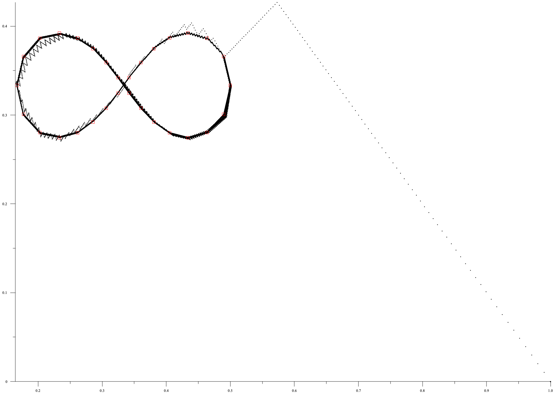
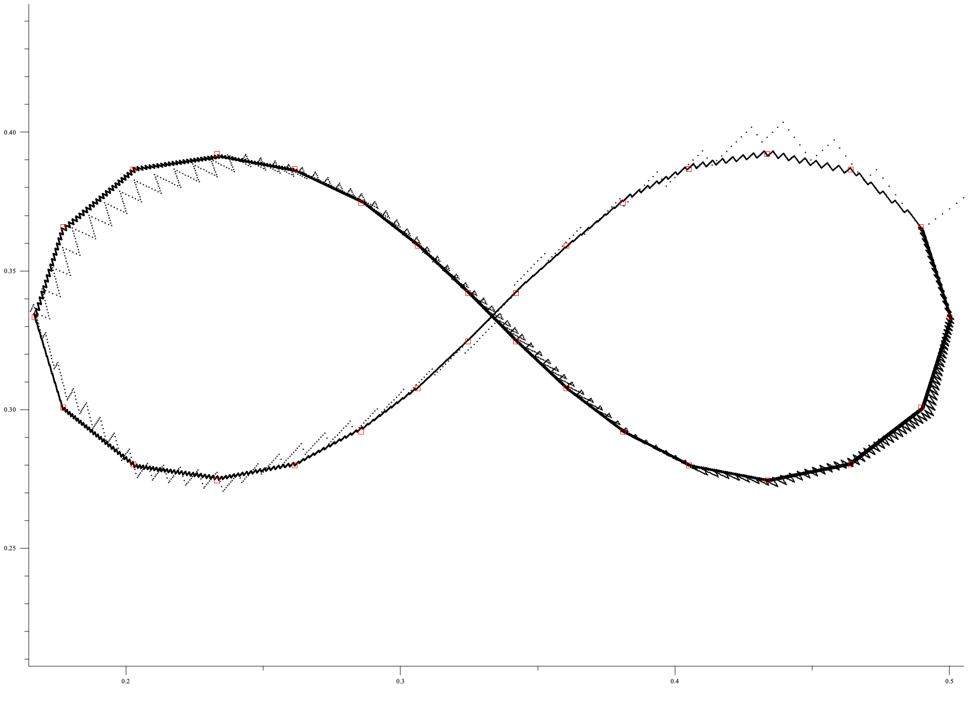
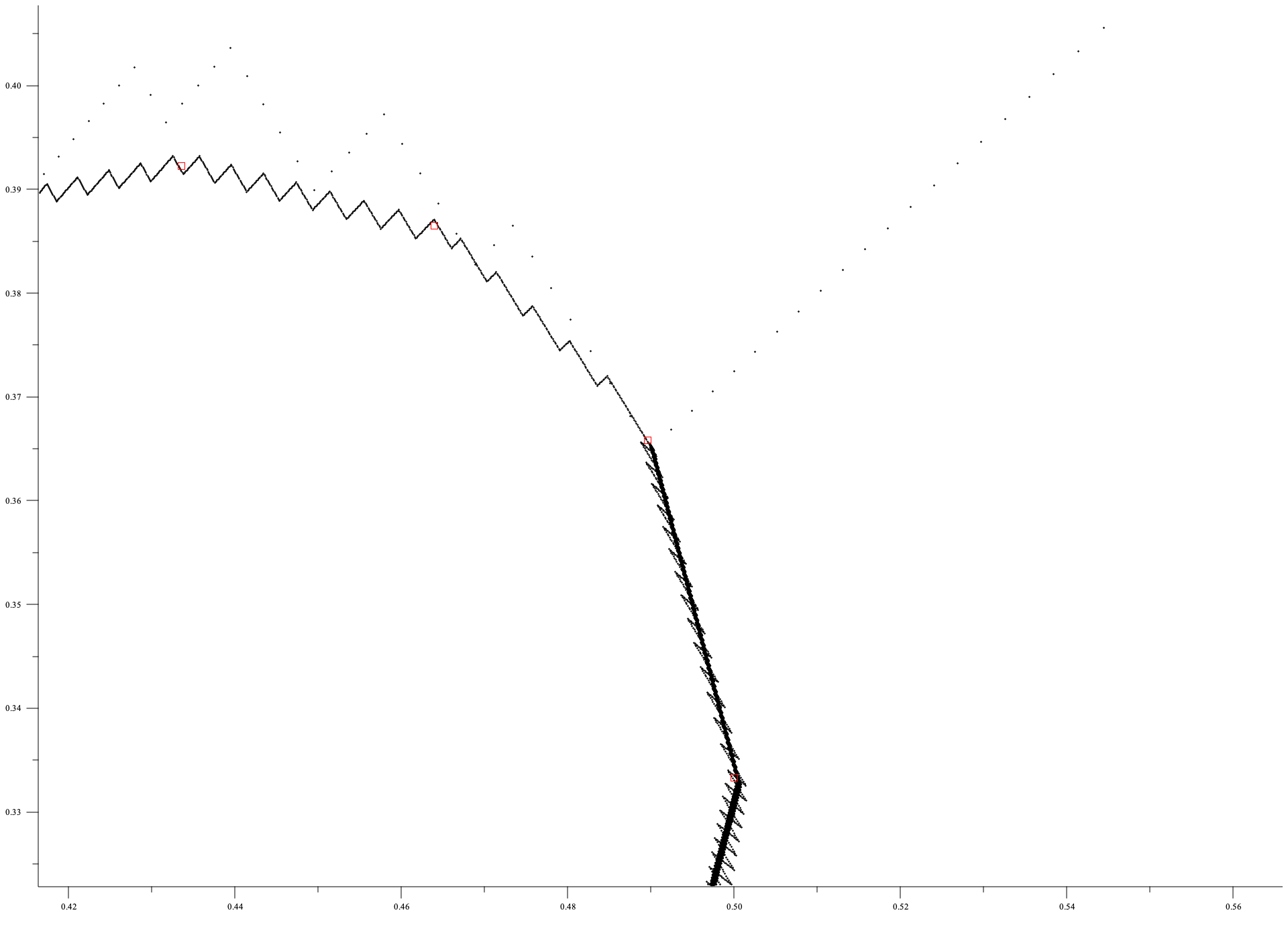
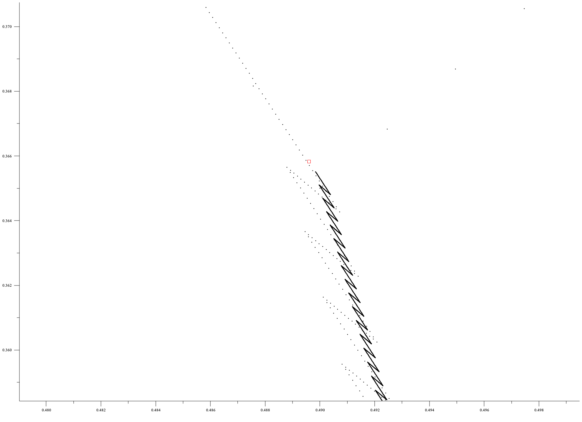
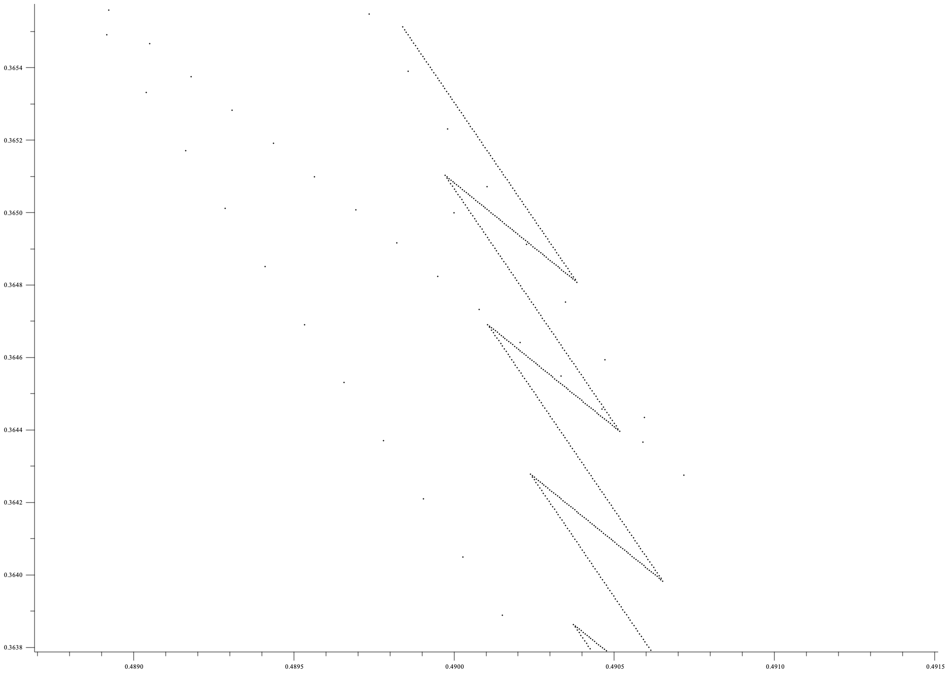
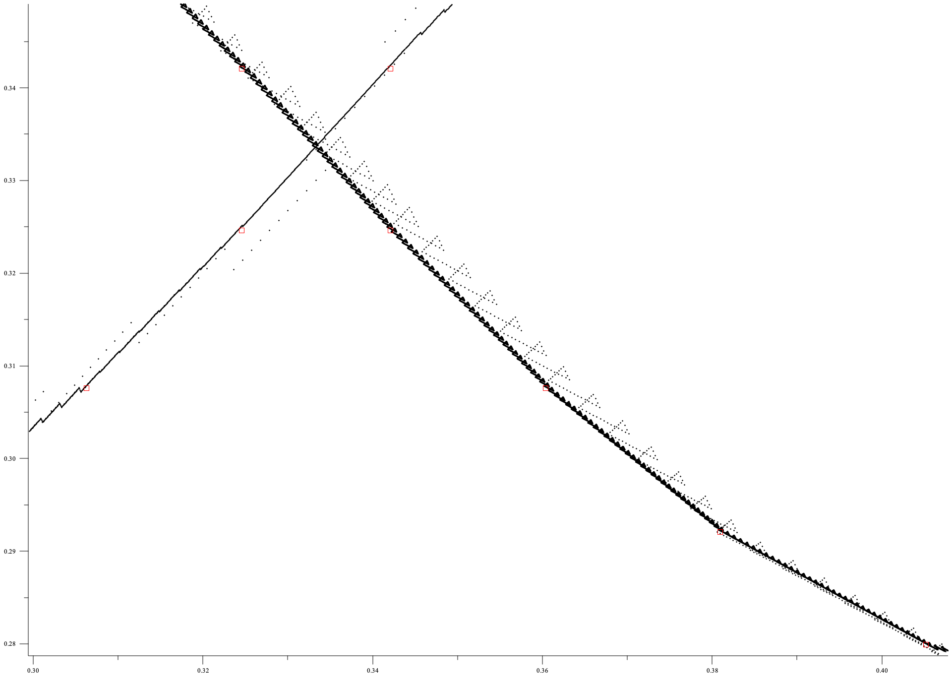
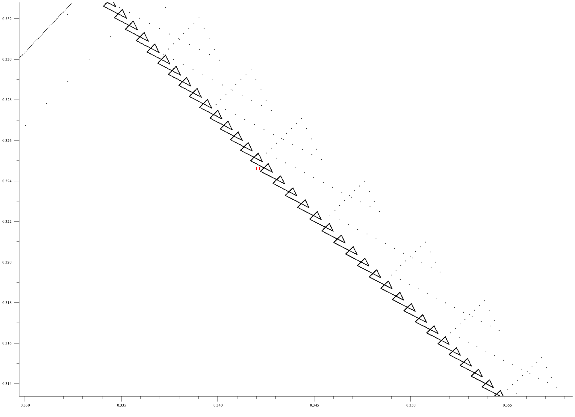
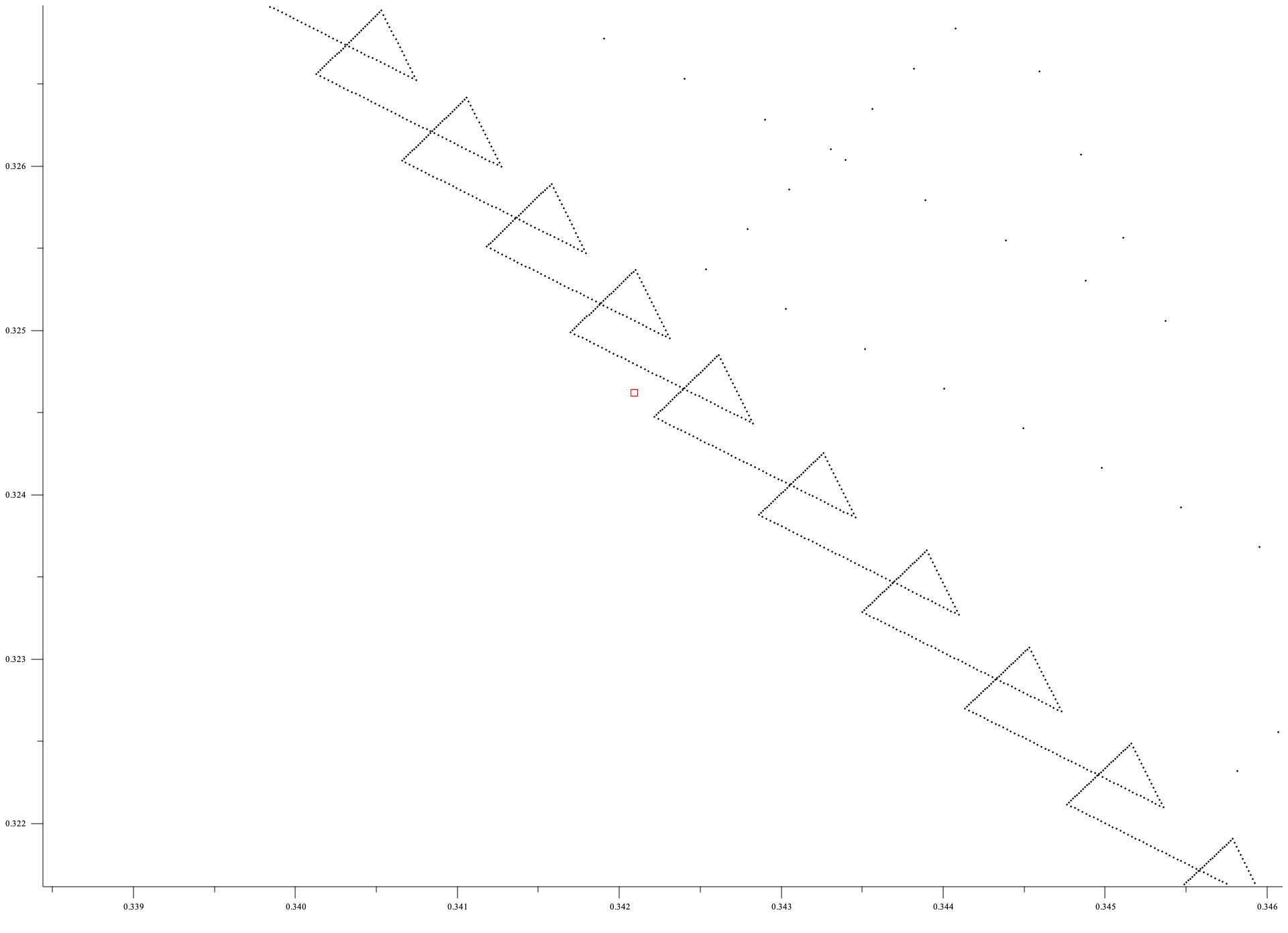
C.12 Construction of such that
How much of the simplex can we cover with ? This question is poorly posed as (it seems) we can only ever construct one dimensional sets that are the set of cluster points of . However, for inducing an upper prevision, all that matters is the convex hull of . We now show the convex hull of can be made as large as conceivable with simpler and more explicit construction:
Lemma C.19.
Suppose . There exists a sequence such that .
Proof.
As before, our proof is constructive. Recall are the vertices (and extreme points) of the -simplex, and . We will construct a sequence such that for all , and all , visits infinitely often. Since we will have achieved the desired result.
We again make use of (13). We will construct a sequence by adding segments () such that for each successive we drive closer and closer towards one of the vertices (). In order to do this, at each we append copies of to the current . Specifically, we construct as follows:
We need to make large enough so that the convex combination coefficient approaches . To that end, consider an increasing function which will further restrict later. The role of is to control as a function of segment number ; that is and thus . With this choice, we have
and thus for all
| (30) |
We demand that so that as increases, the second term in (30) dominates. For any , and thus
where the second line follows from the fact that we constructed such that . But by assumption, and hence for any there exists such that for all ,
That is, for each , each -neighbourhood of is visited infinitely often by the sequence and hence . But since for all we conclude that indeed as required. ∎
A suitable choice of is for some , in which case . An argument as in the proof of Theorem 3.3 would show that . Observe that when , , but for , that is not true, even though .
Appendix D Ivanenko’s Sampling Nets
Ivanenko seeks to abstract away from sequences and hence defines a the notion of a sampling net.
First, we recall the standard definition of a net in topology, which generalizes sequences in an important way. A directed set consists of an arbitrary set and a direction on it, which satisfies the following properties:
-
DIR1.
If , then (reflexivity).
-
DIR2.
If and and , then (transitivity).
-
DIR3.
If , then such that and (upper bound).
That is, is a pre-order and two any two elements there exists a common upper bound.
A net313131Ivanenko calls this “directedness”. is a function , where the domain is a directed set .
Fix a topology on . We say that a point is a cluster point of the net , , if:
As an example, a sequence is a net, where and is the familiar order on the natural numbers.
Define the space of samples from as:
Ivanenko (2010) then calls a net , which takes values in the space of samples from a sampling directedness or sampling net (e.g. in Ivanenko & Labkovskii (2015)). To such a net, Ivanenko associates a net of “frequency counts”:
Furthermore, a corresponding net of relative frequencies can be defined as follows:
where and .
The non-empty closed set of limit points of Ivanenko calls the statistical regularity of the sampling net . The main result in (Ivanenko, 2010) is then the following. Call any non-empty weak* closed subset a regularity.
Proposition D.1 (Ivanenko (2010, Theorem 4.2)).
Any sampling net has a regularity, and any regularity is the regularity of some sampling net [..].
Thus, the concept of a sampling net is in a satisfying one-to-one correspondence to that of a weak* closed set of linear previsions (in (Ivanenko, 2010), finitely additive probabilities). Nonetheless, we remain skeptical about the utility of this concept and raise the question: what is the meaning of a sampling net? Ivanenko & Pasichnichenko (2017) give an intuition: take for example with the familiar order . Then, we could interpret as the frequency of the number of hits in of the observations that are performed at time . Importantly, at any time we could record a totally different number of observations, since that number is itself given by the net . And to obtain the “relative frequencies” at time , we consider only data which was observed at time and completely neglect the past. Contrast this with the case of a sequence: at each time step, we make exactly one observation, and to compute the relative frequencies at time , we use the complete past.
Moreover, in the above example, the directed set with the familiar order was easily intuited. However, Ivanenko’s proof for the direction “to any regularity there exists a corresponding sampling net” is non-constructive in the sense that he uses the exotic directed set
where is the regularity in question and
It is not clear to us what a realistic interpretation for such a sampling net would look like.
Appendix E Pathological or Normal?
Much of the confusion about probability arises because the true depth of the law of large numbers as an extremely hard analytical assertion is not appreciated at all. — Detlef Dürr and Stefan Teufel (2009, p. 62)
When one looks at finite sequences , there is a simple counting argument using the binomial theorem that illustrates that the vast majority of the possible sequences have roughly equal numbers of elements with values of 1 and 2. If one assumes that an infinite sequence is generated i.i.d. then this argument can be used to prove the law of large numbers, which ensures “most” sequences have relative frequencies which converge.
Hence the construction, as illustrated in the present paper, of sequences with divergent relative frequencies naturally raises the question of how contrived they are. That is, are we examining a rare pathology, or something “normal” that we might actually encounter in the world? We will refer to sequences whose relative frequencies converge as “ stochastic sequences” and sequences whose relative frequencies do not converge as “ non-stochastic sequences”323232 This dichotomy would appear clear-cut, but there is a subtlety: there exist sequences such that and are both stochastic, but the joint sequence is non-stochastic (Rivas, 2019); that is, the marginal relative frequencies converge, but the joint relative frequencies do not! .
The classical law of large numbers suggests that indeed “almost all” sequences are stochastic, and therefore, by such reasoning, the non-stochastic sequences with which we have concerned ourselves in the present paper are indeed pathological exceptions. In this appendix we will argue:
-
1.
This very much depends upon what one means by “rare” or “almost all” and there are many choices, and the only real argument in favour of the usual ones (which declare non-stochastic sequences rare) is familiarity — different notions of “typicality” (for that is what is at issue) lead to very different conclusions. Specifically, there are choices (arguably just as “natural” as the familiar ones) which imply that rather than non-stochastic sequences being rare, they are in fact the norm in a very strong sense.
-
2.
Nevertheless, none of the mathematical nuances of the previous point allow one to conclude anything about the empirical prevalence of stochastic or non-stochastic sequences in the world. Indeed, no purely mathematical reasoning allows one to draw such conclusions, unless one wishes to appeal to some conception of a Kantian “synthetic a priori.”
We will first explore what can said from a purely mathematical perspective, illustrating that there is a surprising amount of freedom of choice in precisely posing the problem, and that the choices are consequential. Then in Subsection E.3 we examine the question of prevalence of non-stochastic sequences actually in the world.
E.1 The Mathematical Argument — The Choices to be Made
The classical Law of Large Numbers says “almost all sequences” are stochastic. But the “almost all” claim comes from the mapping of sequences to real numbers in and then making a claim that “almost all” numbers correspond to stochastic sequences. Thus there are at least three choices being made here:
- Mapping from Sequences to Real Numbers
-
The choice of mapping from sequences to real numbers, to enable to use of some notion of typicality on to gauge how common stochastic sequences are.
- Notion of Typicality
-
The notion of typicality to be used (e.g. Cardinality, Hausdorff dimension, Category or Measure).
- Specific Index of Typicality
-
Within the above choice of notion of typicality, the particular choice of typicality index, e.g. the measure or topology that underpins the notion of typicality.
The choices for the classical law of large numbers are 1) -ary positional representation; 2) a -additive measure on ; 3) The Lebesgue measure. As we shall summarize below, each of these three choices substantially affects the theoretical preponderance of non-stochastic sequences.
That there are alternate choices that lead to the unusual conclusion that non-stochastic sequences are “typical” has been known for some time: “This result may be interpreted to mean that the category analogue of the strong law of large numbers is false” (Oxtoby, 1980, p. 85); see also (Méndez, 1981). The significance of this fact has been stressed recently (Seidenfeld et al., 2017; Cisewski et al., 2018). And it has been observed that the introduction of alternate topologies can change whether sequences are stochastic (Khrennikov, 2013). However, the strongest results arise in number theory, motivated by the notion of a “normal number.”
E.2 Notions of Typicality — Cardinality, Dimension, Comeagreness, and Measure
Let (resp. ) denote the set of stochastic (resp. non-stochastic) sequences . That is, and . (For simplicity, and alignment with Appendix C, we restrict ourselves to sequences whose domain is .)
In order to make a claim regarding the relative preponderance of stochastic versus non-stochastic sequences, they are often mapped onto the unit interval.333333The only attempts to judge the relative sizes of and which do not rely on such a mapping are described in the first and third of the cases listed below, and rely upon imposing a topology directly on the set of sequences . In such cases, the question of relative preponderance of classes of sequences is reduced to that of a question concerning the relative preponderance of classes of subsets of . The question then arises of how to measure the size of such subsets. Unlike in the finite case mentioned above, merely counting (i.e. determining the cardinality of the respective subsets) is hardly adequate, as it is easy to argue that . There are three notions that have been used to compare the size of and :
- Measure
-
A countably additive measure, usually the Lebesgue measure on .
- Meagre / Comeagre
-
A subset of a topological space is meagre if it is a countable union of nowehre dense sets (i.e. sets whose closure has empty interior). A set is comeagre (residual) if is meagre.
- Dimension
-
A variety of fractal dimensions, such as the Hausdorff dimension, have also been used to judge the size of non-stochastic sequences (and the numbers they induce); however for space considerations we omit discussion of these results343434 See for example (Eggleston, 1949; Olsen, 2004; Gu & Lutz, 2011; Bishop & Peres, 2017; Albeverio et al., 2017). .
Some of the results obtained in the literature are summarized below. The object is not to state them in an entirely formal manner, or even to describe them in their full generality. Rather we simply wish to show the diversity of conclusions available by tweaking the three choices enumerated above. If no representation is mentioned, the usual -ary positional representation is used, whereby is constructed from via (the term is required because our sequences map to ). Obviously every maps to some ; and every corresponds to at least one (recalling we have to handle the situation that, when for example, , where means that is repeated infinitely, and thus there are two sequences such that ). 353535This non-uniqueness of the representation will not affect the results below because and is of cardinality , whereas . Let and .
- Most (Lebesgue measure) sequences are stochastic
-
This is the classical strong law of large numbers. If denotes the Lebesgue measure on , then the claim is that .
- Most (comeagre) sequences are non-stochastic
-
Let and equipped with the product topology. As a set . Then is comeagre (Oxtoby, 1980).
- Most (comeagre) sequences are stochastic
-
With different choices of topology, the opposite conclusion holds — there are topologies such that is comeagre (Calude et al., 2003).
- Most (comeagre) sequences are extremely non-stochastic
-
Let denote the subset of of corresponding to which satisfy These sequences are (justifiably) called extremely non-stochastic; the sequence constructed in Subsection C.12 is an example. Then the set is comeagre in the usual topology of real numbers (Calude & Zamfirescu, 1999); confer (Calude, 2002, section 7.3).
- Most (comeagre) sequences are perversely non-stochastic
-
Denote the set of perversely nonstochastic sequences . Observe . Let (what Olsen (2004) calls “extremely non-normal numbers”, but we use “extremely” for the larger set ). Then is comeagre (in the usual topology of real numbers) (Aveni & Leonetti, 2022; Olsen, 2004). An even stronger result holds. Let denote a (not necessarily uniform) finite averaging operator and let and . Observe and . Then is also comeagre (Stylianou, 2020)!
- Most (Lebesgue measure) sequences are non-stochastic
-
There exist a range of representations of real numbers called -representations ( is a matrix valued parameter of the representation); see (Albeverio et al., 2005, Section 4) for details. Let denote the -representation of a sequence , and and . Then there exist such that . (Albeverio et al., 2005, p. 627). Thus if the size of is judged via certain representations, Lebesgue almost all sequences are non-stochastic!
An obvious conclusion to draw from the above examples is that in answering the question of the preponderance of non-stochastic sequences, one can get essentially whatever answer one wants by choosing a range of different precise formulations of the question. At the very least, this should make us skeptical of any purely mathematical attempts to reason whether one might expect to encounter non-stochastic sequences in practice — the topic to which we now turn.
E.3 Typical Real Sequences
The laws of large numbers cannot be applied for describing the statistical stabilization of frequencies in sampling experiments. — Andrei Khrennikov (2009, p. 20)
What do the above points imply about the likelihood one will encounter stochastic or non-stochastic sequences when performing real measurements?
Nothing.
This is not to say that in actuality we will often encounter non-stochastic sequences. Rather our point is that no amount of purely theoretical reasoning will be able to tell us in advance how “likely” it is to do so. What is at issue is whether stochastic sequences are in fact “typical” in our world.
Perhaps the most surprising thing about the mathematical results summarized above is the extent to which different notions of typicality affect the conclusions. This raises the question of whether some notions of typicality are more justified when wishing to consider real sequences that have been measured in the world. In the study of physics (especially aspects of physics that are apparently intrinsically statistical) such questions have been raised, and below we briefly summarize what is known.
Traditionally, “probability” is considered as a primitive, and notions of typicality are derived from that in terms of their “probability” of occurring. And the above examples illustrate that attempts to argue for the Lebesgue measure having a privileged role as the “right” notion of typicality are barking up the wrong tree; confer (Pitowsky, 2012). But this will not do for our question. Typicality is a more fundamental notion (Galvan, 2006; 2007) — arguably the “mother of all” notions of probability (Goldstein, 2012). Typicality is at the core of questions of non-stochastic randomness in physics, thus (consistent with the perspective of the present paper) leading to non-additive measures of typicality (Galvan, 2022) (essentially defining a measure of typicality inspired by a coherent upper probability) which allows the extension to notions of mutual typicality necessary to reason about situations such as that referred to in footnote 32.
In fact, typicality plays an even stronger role than answering questions regarding the preponderance of non-stochastic sequences. As Dürr & Struyve (2021, p. 36) observe “the notion of typicality is necessary to understand what the statistical predictions of a physical theory really mean.” They note that the usual appeal to the law of large numbers misses the point because while its conclusion is true (convergence of relative frequencies) if one sees typical sequences, but “What needs to be explained is why we only see typical sequences! That’s actually the deep question underlying the meaning of probability theory from its very beginning …” (Dürr & Struyve, 2021, p. 37). In classical mechanics, appeal to Liouville’s theorem suggests an “invariant measure” as being a natural choice; in the quantum realm, there is an analogous choice (invariant to Bohmian flow) (Dürr & Struyve, 2021, p. 41). But these situations are rather special from the perspective of a statistician. The situation is well summarized by Dürr (2001, p. 130): “What is typicality? It is a notion for defining the smallness of sets of (mathematically inevitable) exceptions and thus permitting the formulation of law of large numbers type statements. Smallness is usually defined in terms of a measure. What determines the measure? In physics, the physical theory.” Confer (Dürr & Teufel, 2009, Chapter 4) who observe that from a scientific perspective (where one wants to make claims about the world) establishing the pre-conditions for the law of large numbers to hold is “exceedingly difficult”363636The example they give is for the Galton board, or quincunx, a device often appealed to in order to teach the reality of the central limit theorem — an even stronger claim than the law of large numbers. The irony is that it is rarely checked empirically. And when it has been, it has been found to be untrue! (Bagnold, 1983, Figure 8)..
Very well one might say, but the arguments in favor of typicality of non-stochastic sequences given above all rely on topological arguments, or unusual encodings of sequences to numbers. What is the justification for topological notions of typicality when considering sequences of measurements obtained from the world? Sklar (2000, p. 270) has actually argued that the topological perspective might offer a foundational perspective with fewer opportunities for claims of arbitrariness than measure theoretical approaches. See also (Sklar, 1995, p. 185) and the discussion in (Guttmann, 1999, Chapter 4) which reframes the problem away from typicality to viewing the whole question from an approximation perspective where the notion of smallness of sets is naturally one of meagreness. Our point is that even within the restricted realm of physics, there are compelling arguments at least not to take the measure-based notion of typicality for granted. Once that is accepted, non-stochastic sequences seem less unusual.
E.4 Violations of the Law of Large Numbers
A typical universe is in equilibrium; but “our universe is atypical or in non-equilibrium” (Dürr & Teufel, 2009, p. 81) and “what renders knowledge at all possible is nonequilibrium” (Dürr et al., 1992, p. 886) so we should not be surprised if it is not “typical”. And indeed that is what we see as long as we look: “The so-called law of large numbers is also invalid for social systems with finite elements during transition” (Chen, 1991). Gorban (2011; 2017; 2018) has documented many examples of real phenomena failing to be statistically stable. Such failures are held to explain departures from “normal” distributions (Philip & Watson, 1987). But more importantly, they mean we should not expect even convergence of relative frequencies in non-equilibrium situations.
Such was the conclusion of Prigogine in his ground-breaking studies of non-equilibrium thermodynamics where he spoke of a “breakdown of the ‘law of large numbers”’ (Nicolis & Prigogine, 1977, p. 9 and 228); see also (Prigogine, 1978, p. 781), (Prigogine & Stengers, 1985, p. 180) and (Prigogine, 1980, p. 131). And more recently, studies of the use of machine learning systems “in the wild” have recognized that non-stochasticity is not so exotic after all (Katsikopoulos et al., 2021). Thus perhaps its time to downgrade this “law” of nature.
E.5 Repeal of the Law of Large Numbers
A typical universe shows statistical regularities as we perceive them in a long run of coin tosses. It looks as if objective chance is at work, while in truth it is not. There is no chance. That is the basis of mathematical probability theory. — Detlef Dürr and Stefan Teufel (2009, p. 64).
Desrosières (1998) in his history of statistical reasoning has observed the awe with which stable frequencies were viewed when they were first encountered; the effect been interpreted as a hidden divine order373737“I know of scarcely anything so apt to impress the imagination as the wonderful form of cosmic order expressed by the ‘Law of Frequency of Error.’ The law would have been personified by the Greeks and deified, if they had known of it. It reigns with serenity and in complete self-effacement amidst the wildest confusion. The huger the mob, and the greater the apparent anarchy, the more perfect is its sway. It is the supreme law of Unreason. Whenever a large sample of chaotic elements are taken in hand and marshalled in the order of their magnitude, an unsuspected and most beautiful form of regularity proves to have been latent all along.” (Galton, 1889, p. 66). See also (Rose, 2016) for a recent discussion on statistical normality. . And indeed in many practical situations, stable frequencies do arise. But that does not mean we should take such situations as the only ones that can occur. We may well legitimately call them “normal.” But we can better understand the normal by studying the pathological (Canguilhem, 1978, p. 19–20). Ironically in his attempt to clarify the notion of “normal” Canguilhem (1978, p. 103) considered whether “normal” was simply “average” and concluded “the concepts of norm and average must be considered as two different concepts”. As we have seen, averages can indeed be far from normal, and potentially quite often.
Perhaps we have been misled by the strange name given to the famous theorem we are considering: by calling it a “law” we are inheriting a lot of baggage as to what we mean by that, baggage that has been traced to notions of divine origin (Zilsel, 1942)383838The contrary views regarding the historical origin of the notion of a scientific law (Milton, 1981; Ruby, 1986; Weinert, 1995) do not contradict our point. of lawfulness. And we hanker after lawfulness:
We …naturally hope that the world is orderly. We like it that way… All of us …find this idea sustaining. It controls confusion, it makes the world seem more intelligible. But suppose the world should happen in fact to be not very intelligible? Or suppose merely that we do not know it to be so? Might it not then be our duty to admit these distressing facts? (Midgley, 2013, p. 199)
Perhaps the theory of imprecise probabilities presented in this paper which we have grounded in the instability of relative frequencies may help us to admit this “distressing fact.” It does suggest to us that the law of large numbers, while a fine and true theorem, as a “law” might be in need of repealing.