Differential Privacy with Higher Utility through Non-identical Additive Noise

Abstract

Differential privacy is typically ensured by perturbation with additive noise that is sampled from a known distribution. Conventionally, independent and identically distributed (i.i.d.) noise samples are added to each coordinate. In this work, propose to add noise which is independent, but not identically distributed (i.n.i.d.) across the coordinates. In particular, we study the i.n.i.d. Gaussian and Laplace mechanisms and obtain the conditions under which these mechanisms guarantee privacy. The optimal choice of parameters that ensure these conditions are derived theoretically. Theoretical analyses and numerical simulations show that the i.n.i.d. mechanisms achieve higher utility for the given privacy requirements compared to their i.i.d. counterparts.

I Introduction

Differential privacy (DP) is a mathematical formulation that safeguards an individual’s privacy while releasing query responses on databases [1]. It facilitates the learning of the patterns in the population while ensuring the privacy of an individual. The parameters $\epsilon$ and $\delta\hskip 0.50003pt$, respectively the privacy budget and privacy leakage capture the privacy constraints. The formal definitions of DP and its mechanisms are deferred to Section II. Differential privacy has wide-ranging applications; it is used to provide privacy guarantees on learning problems such as empirical risk minimization [2], data mining [3], low-rank matrix completion [4], clustering [5] etc.

Additive noise mechanism randomizes the result of a real-valued query on the dataset by adding noise sampled from a known distribution and ensures privacy. When the query response is $K$-dimensional, the convention is to add independent and identically distributed (i.i.d.) noise samples to each of the coordinates; hence, the accuracy translates to the variance of this i.i.d. noise. Note that there is always a trade-off between privacy and utility. Stronger privacy guarantee can be achieved by adding noise of larger variance; however, this will affect the accuracy of the outcome.

Over the years, several noise distributions have been considered for differential privacy and the privacy guarantees of such mechanisms have been documented. Gaussian mechanism that adds i.i.d. noise from $\mathcal{N}(0,\sigma^{2})$ is a popular mechanism that has been studied extensively. Various sufficient conditions that directly provide the scale parameter $\sigma$ satisfying the given privacy constraints, are available [6, 1, 7]. However, the necessary and sufficient condition in [8] has been shown to provide the smallest variance $\sigma^{2}$ that ensures $(\epsilon,\delta)$-DP, though not in closed form.

Laplace mechanism is another popular mechanism that, unlike Gaussian, is capable of ensuring the stronger notion of DP with $\delta=0$. However, Gaussian mechanism typically adds noise of smaller variance compared to the Laplace mechanism when employed for high dimensional queries [9]. This is because the $\ell_{1}$-sensitivity, which determines the variance of Laplace noise, increases faster with the dimension than the $\ell_{2}$-sensitivity associated with Gaussian noise.

Similar to Laplace, logistic mechanism [10, 11] can also ensure the stronger $\epsilon$-DP. Subbotin density has also been considered for sampling the additive noise [12]. Recently proposed Offset Symmetric Gaussian Tails (OSGT) mechanism [13] and Flipped Huber mechanism [14] add noise sampled from sub-Gaussian distributions and are shown to provide better accuracy than the Gaussian mechanism for the given privacy constraints. However, determination of noise parameters in these mechanisms is complex, especially when the dimension of the query response is very large. Thus, Gaussian and Laplace mechanisms still remain the popular choices since the scale parameter for the given privacy constraints can be determined easily.

To our best knowledge, existing works have only considered the addition of i.i.d. noise to the coordinates of the query result. This is not a suitable choice, especially when the individual coordinates of the query are of different sensitivities to the replacement of a single data record in the dataset. In this work, we investigate whether adding independent, but non-identically distributed (i.n.i.d.) noise samples instead of i.i.d. samples provides any gain in terms of utility while guaranteeing privacy. Specifically, we introduce the i.n.i.d. variants of the two popular noise mechanisms, namely the Gaussian and Laplace mechanisms and provide both theoretical and empirical results to illustrate the benefits of i.n.i.d. noise addition.

I-A Contributions

The major contributions are listed below.

1. We propose to add the noise that is i.n.i.d. across the coordinates of the query response so that privacy is ensured with lesser perturbation than i.i.d. noise.

2. In specific, we consider i.n.i.d. Gaussian and Laplace mechanisms and the corresponding $(\epsilon,\delta)$-DP and $\epsilon$-DP guarantees are derived.

3. The optimal choices of coordinate-wise scale parameters for these mechanisms are derived that improve the accuracy/utility compared to the i.i.d. variants, leveraging on the disparity in the coordinate-wise sensitivities.

4. Through theoretical analyses and simulations, we show that the i.n.i.d. noise, with the proposed set of scale parameters, provides high accuracy over the i.i.d. noise.

To the best of our knowledge, ours is the first work to formally introduce the i.n.i.d. mechanisms for differential privacy and show that i.n.i.d. noise can give higher utility than i.i.d. noise for the same privacy requirements with the appropriate choice of the noise parameters.

I-B Basic notations

In this article, $\log(\cdot)$ denotes the natural logarithm. The positive part of a real number ${a}$ is denoted as $[{a}]_{+}=\max({a},0)\hskip 0.50003pt$. $\mathbb{R}_{++}$ indicates the set of positive real numbers, $(0,\infty)\hskip 0.50003pt$, which with the inclusion of 0 is denoted as $\mathbb{R}_{+}\hskip 0.50003pt$. We use bold-face letters to denote the vectors. The operator $\left\lVert\cdot\right\rVert_{p}\hskip 0.50003pt$ provides the $\ell_{p}$-norm of a vector. The vector of all ones in $\mathbb{R}^{K}$ is denoted as $\mathbf{1}_{K}$. The diagonal matrix formed by the elements of vector $\mathbf{{r}}\in\mathbb{R}^{K}$ is written as $\operatorname{diag}(\mathbf{{r}})$ and $\mathbf{{r}}^{\circ p}$ denotes $p$-th Hadamard power, $\mathbf{{r}}^{\circ p}=[\,{r}_{1}^{p}\ {r}_{2}^{p}\ \cdots\ {r}_{K}^{p}\,]^{\top}\hskip 0.50003pt$. The probability measure is denoted by $\mathbb{P}\{\cdot\}$ and $\mathbb{E}[\hskip 0.50003pt\cdot\hskip 0.50003pt]$ indicates the expectation. The probability density function (PDF) and the cumulative distribution function (CDF) of the random variable $T$ are respectively denoted as ${g}_{\hskip 0.35002ptT}(\cdot)$ and ${G}_{\hskip 0.35002ptT}(\cdot)$. The Gaussian (or normal) distribution with variance $\sigma^{2}$ that is centred at ${\theta}$ is denoted by $\mathcal{N}({\theta},\sigma^{2})$ and $\mathcal{L}({\theta},\beta)$ denotes Laplace (or bilateral exponential) distribution with mean ${\theta}$ and scale parameter $\beta\hskip 0.50003pt$. Let ${Q}(\cdot)$ denote the complementary CDF of the standard Gaussian distribution $\mathcal{N}(0,1)$.

II Background and i.i.d. noise mechanisms

We now provide some definitions pertaining to differential privacy and also introduce a few notations that we will be using in this article. Let $\mathcal{X}$ be the space of datasets. The query function ${f}:\mathcal{X}\to\mathcal{Y}$ acts on dataset $\mathcal{D}\in\mathcal{X}$ and provides the query response ${f}(\mathcal{D})\hskip 0.50003pt$. If a pair of datasets differ by only a single data record, we call them neighbouring datasets; when $\mathcal{D}$ and $\widecheck{\mathcal{D}}$ are neighbouring datasets in $\mathcal{X}\hskip 0.50003pt$, we write $\mathcal{D}\hskip 1.00006pt{\rotatebox[origin={c}]{90.0}{\footnotesize{$\rangle\langle\!$}}}_{{}_{\mathcal{X}}}\widecheck{\mathcal{D}}$.

Definition 1.

​[1] The randomized mechanism $\mathcal{M}:\mathcal{X}\to\mathcal{Y}$ is said to guarantee $(\epsilon,\delta)$-differential privacy ($(\epsilon,\delta)$-DP in short) if for every measurable set $\mathcal{E}$ in $\mathcal{Y}\hskip 0.50003pt$ and every pair of neighbouring datasets $\mathcal{D}\hskip 1.00006pt{\rotatebox[origin={c}]{90.0}{\footnotesize{$\rangle\langle\!$}}}_{{}_{\mathcal{X}}}\widecheck{\mathcal{D}}$,

$$\mathbb{P}\{\mathcal{M}(\mathcal{D})\in\mathcal{E}\}\leq e^{\epsilon}\hskip 1.00006pt\mathbb{P}\{\mathcal{M}(\widecheck{\mathcal{D}})\in\mathcal{E}\}+\delta$$ (1)

where $\epsilon\geq 0$ and $\delta\in[0,1]$ are respectively the privacy budget and privacy leakage parameters. When $\delta=0\hskip 0.50003pt$, the mechanism is said to guarantee pure DP or $\epsilon$-DP.

The notion of privacy loss [15] encapsulates the divergence between the mechanism’s outputs on the neighbouring datasets as a univariate random variable. Let us denote the probability measures associated with $\mathcal{M}(\mathcal{D})$ and $\mathcal{M}(\widecheck{\mathcal{D}})$ respectively as ${\mu}$ and $\widecheck{{\mu}}$ and assume that ${\mu}$ is absolutely continuous with respect to $\widecheck{{\mu}}\hskip 0.50003pt$, i.e., ${\mu}\ll\widecheck{{\mu}}$ (for generalization, see [16]).

Definition 2.

The random variable $\mathfrak{L}^{\mathcal{D},\widecheck{\mathcal{D}}}_{{}_{\mathcal{M}}}=\log\frac{\mathrm{d}{\mu}}{\mathrm{d}\widecheck{{\mu}}}(\mathbf{{V}})\hskip 0.50003pt$, where $\mathbf{{V}}\sim{\mu}\hskip 0.50003pt$, is known as the privacy loss random variable of the mechanism $\mathcal{M}$ on the neighbouring datasets $\mathcal{D}\hskip 1.00006pt{\rotatebox[origin={c}]{90.0}{\footnotesize{$\rangle\langle\!$}}}_{{}_{\mathcal{X}}}\widecheck{\mathcal{D}}$. The corresponding privacy loss function is given by $\log\frac{\mathrm{d}{\mu}}{\mathrm{d}\widecheck{{\mu}}}\hskip 0.50003pt$.

Whenever the density functions of $\mathcal{M}(\mathcal{D})$ and $\mathcal{M}(\widecheck{\mathcal{D}})$ are defined, the privacy loss function reduces to the logarithm of their ratio. The following expression from [8] is an equivalent condition for $(\epsilon,\delta)$-DP in terms of the privacy loss random variables.

$$\begin{array}[]{c}\sup\\[-12.50002pt] {}_{\mathcal{D}\hskip 0.70004pt{\rotatebox[origin={c}]{90.0}{\scriptsize{$\rangle\langle\!$}}}_{{}_{\mathcal{X}}}\widecheck{\mathcal{D}}}\end{array}\!\,\mathbb{P}\big{\{}\mathfrak{L}^{\mathcal{D},\widecheck{\mathcal{D}}}_{{}_{\mathcal{M}}}>\epsilon\big{\}}-e^{\epsilon}\hskip 1.00006pt\mathbb{P}\big{\{}\mathfrak{L}^{\widecheck{\mathcal{D}},\mathcal{D}}_{{}_{\mathcal{M}}}<-\epsilon\big{\}}\leq\delta\hskip 1.00006pt.$$ (2)

This characterization of DP through privacy losses makes the analysis easier whenever the privacy losses are sufficiently simple. We observe one such scenario in the following subsection for the case of additive noise mechanisms, where the privacy loss can be redefined simply in terms of noise density.

II-A Additive noise mechanism

A direct way to randomize the query response that is a numeric vector is to add noise to it.

Definition 3 (Additive noise mechanism).

Let ${f}:\mathcal{X}\rightarrow\mathbb{R}^{K}$ be the $K$-dimensional, real-valued query function. The additive noise mechanism imparts differential privacy by perturbing the query output for the dataset $\mathcal{D}$ as $\mathcal{M}(\mathcal{D})={f}(\mathcal{D})+\mathbf{t}\hskip 0.50003pt$, where $\mathbf{t}=[{t}_{1}\ {t}_{2}\ \cdots\ {t}_{K}]^{\top}\in\mathbb{R}^{K}$ is the noise that is sampled from a known distribution with CDF ${G}_{\hskip 0.35002pt\mathbf{T}}$ and PDF ${g}_{\hskip 0.35002pt\mathbf{T}}\hskip 0.50003pt$.

Conventionally, ${t}_{i},\ i=1,\,2,\,\ldots,\,K$ are i.i.d. noise samples drawn from some univariate distribution. The amount of noise added is determined by the privacy parameters $\epsilon$ and $\delta\hskip 0.50003pt$. Along with these, the sensitivity of the query function also impacts the variance of added noise.

Definition 4 (Sensitivity).

For the real-valued, $K$-dimensional query function ${f}:\mathcal{X}\rightarrow\mathbb{R}^{K}$, the $\ell_{p}$-sensitivity is defined as

$$\Delta_{p}=\begin{array}[]{c}\sup\\[-12.50002pt] {}_{\mathcal{D}\hskip 0.70004pt{\rotatebox[origin={c}]{90.0}{\scriptsize{$\rangle\langle\!$}}}_{{}_{\mathcal{X}}}\widecheck{\mathcal{D}}}\end{array}\!\,\big{\|}{f}(\mathcal{D})-{f}(\widecheck{\mathcal{D}})\big{\|}_{p}\,,\quad p\in[1,\infty]\hskip 1.00006pt.$$ (3)

The sensitivity profile is the vector of coordinate-wise sensitivities, $\boldsymbol{{\lambda}}=[\,{\lambda}_{1}\ {\lambda}_{2}\ \cdots\ {\lambda}_{K}\,]^{\top}$, where

$${\lambda}_{i}=\begin{array}[]{c}\sup\\[-12.50002pt] {}_{\mathcal{D}\hskip 0.70004pt{\rotatebox[origin={c}]{90.0}{\scriptsize{$\rangle\langle\!$}}}_{{}_{\mathcal{X}}}\widecheck{\mathcal{D}}}\end{array}\!\big{|}[{f}(\mathcal{D})-{f}(\widecheck{\mathcal{D}})]_{i}\big{|}$$

is the sensitivity of the $i$-th coordinate. Hence, $\Delta_{p}=\left\lVert\boldsymbol{{\lambda}}\right\rVert_{p}\hskip 0.50003pt$.

Thus, sensitivity indicates the maximum magnitude of change that the true response incurs when a single entry of the dataset is replaced. Using the equivalence of norms [17], we have

$$\Delta_{{q}}\leq{K}^{{\left[\hskip 0.35002pt1/{q}\hskip 0.35002pt-\hskip 0.35002pt1/{r}\hskip 0.35002pt\right]_{+}}}_{\stackrel{{\scriptstyle}}{{}}}\!\times\Delta_{{r}}\,,\quad\,\ \forall\,{q},\,{r}\in[1,\infty]\hskip 1.00006pt.$$ (4)

We observe that $\Delta_{{q}}\leq\Delta_{{r}}\,\ \forall\,{r}\geq{q}\hskip 0.50003pt$, and hence, $\Delta_{p}$ is monotonic decreasing in ${p}\hskip 0.50003pt$.

Next, we define the equivalent privacy loss for the additive noise mechanism. Let $\mathbf{{z}}={f}(\mathcal{D})$ and $\widecheck{\mathbf{{z}}}={f}(\widecheck{\mathcal{D}})$ denote the true responses to the query on the neighbouring datasets $\mathcal{D}\hskip 1.00006pt{\rotatebox[origin={c}]{90.0}{\footnotesize{$\rangle\langle\!$}}}_{{}_{\mathcal{X}}}\widecheck{\mathcal{D}}\hskip 0.50003pt$ and let $\mathbf{d}=\mathbf{{z}}-\widecheck{\mathbf{{z}}}\hskip 0.50003pt$. Also, let $\mathbf{T}$ be the random vector that models the additive noise. Thus, the random vectors corresponding to the mechanism’s outputs for $\mathcal{D}$ and $\widecheck{\mathcal{D}}$ are respectively $\mathbf{{V}}=\mathbf{{z}}+\mathbf{T}$ and $\widecheck{\mathbf{{V}}}=\widecheck{\mathbf{{z}}}+\mathbf{T}\hskip 0.50003pt$.

Hence, we have the output densities as ${g}_{\hskip 0.35002pt\mathbf{{V}}}(\mathbf{{v}})={g}_{\hskip 0.35002pt\mathbf{T}}(\mathbf{t})$ and ${g}_{\hskip 0.35002pt\widecheck{\mathbf{{V}}}}(\mathbf{{v}})={{g}_{\hskip 0.35002pt\mathbf{T}}(\mathbf{t}+\mathbf{d})}\hskip 0.50003pt$, where $\mathbf{t}=\mathbf{{v}}-\mathbf{{z}}\hskip 0.50003pt$. The equivalent privacy loss function is given by ${\zeta}_{\hskip 0.35002pt\mathbf{d}}(\mathbf{t})=\log\frac{{g}_{\hskip 0.25002pt\mathbf{T}}(\mathbf{t})}{{g}_{\hskip 0.25002pt\mathbf{T}}(\mathbf{t}+\mathbf{d})}\hskip 0.50003pt$. It is evident that the random variable ${\zeta}_{\hskip 0.35002pt\mathbf{d}}(\mathbf{T})\hskip 0.50003pt$, where $\mathbf{T}\sim{G}_{\hskip 0.35002pt\mathbf{T}}$ is probabilistically equivalent to $\mathfrak{L}^{\mathcal{D},\widecheck{\mathcal{D}}}_{{}_{\mathcal{M}}}\hskip 0.50003pt$. Therefore, we can express the necessary and sufficient condition for the additive noise mechanism to guarantee $(\epsilon,\delta)$-DP using the equivalent privacy losses as

$$\begin{array}[]{c}\sup\\[-12.50002pt] {}_{\mathcal{D}\hskip 0.70004pt{\rotatebox[origin={c}]{90.0}{\scriptsize{$\rangle\langle\!$}}}_{{}_{\mathcal{X}}}\widecheck{\mathcal{D}}}\end{array}\!\mathbb{P}\{{\zeta}_{\hskip 0.35002pt\mathbf{d}}(\mathbf{T})\geq\epsilon\}-e^{\epsilon}\hskip 1.00006pt\mathbb{P}\{{\zeta}_{\hskip 0.35002pt-\mathbf{d}}(\mathbf{T})\leq-\epsilon\}\leq\delta\hskip 1.00006pt,$$ (5)

which resembles (2).

II-A1 Classical Gaussian mechanism

The following lemma provides the privacy guarantees of the i.i.d. Gaussian mechanism.

Lemma 1.

​[8] The Gaussian mechanism that adds i.i.d. noise sampled from $\mathcal{N}(0,\sigma^{2})$ to each of the $K$ coordinates of the query response is $(\epsilon,\delta)$-differentially private if and only if

$${Q}\!\left(\tfrac{\sigma\epsilon}{\Delta_{2}}-\tfrac{\Delta_{2}}{2\sigma}\right)\!-e^{\epsilon}{Q}\!\left(\tfrac{\sigma\epsilon}{\Delta_{2}}+\tfrac{\Delta_{2}}{2\sigma}\right)\!\hskip 1.00006pt\leq\delta\hskip 1.00006pt,$$

where $\Delta_{2}$ is the $\ell_{2}$-sensitivity of the query.

The smallest $\sigma$ that satisfies the condition in the above theorem corresponds to the optimal i.i.d. Gaussian noise that results in the smallest perturbation of query output. Such a scale parameter cannot be determined in closed form but can be obtained numerically [8].

II-A2 Classical Laplace mechanism

The necessary and sufficient condition for the i.i.d. Laplace mechanism that adds noise samples from $\mathcal{L}(0,\beta)\hskip 0.50003pt$ to guarantee $(\epsilon,\delta)$-DP [16, 11] is $\!\left[1-\exp\!\left(\tfrac{1}{2}(\epsilon-\Delta_{1}/\beta)\right)\right]_{+}\!\hskip 0.50003pt\leq\delta\hskip 0.50003pt$. Because of the exponential tails of the noise distribution, the Laplace mechanism, unlike the Gaussian mechanism, is also capable of ensuring pure DP [18] as stated in the following Lemma.

Lemma 2.

​[19] The i.i.d. Laplace mechanism that adds $K$ independent noise samples from $\mathcal{L}(0,\beta)$ to each coordinate of the query response guarantees $\epsilon$-differentially private for $\epsilon\geq\tfrac{\Delta_{1}}{\beta}\hskip 0.50003pt$, where $\Delta_{1}$ is the $\ell_{1}$-sensitivity of the query.

Hence, the Laplace noise of scale $\tfrac{\Delta_{1}}{\epsilon}$ corresponds to the minimum level of i.i.d. noise that is needed for $\epsilon$-DP. Note that the classical Gaussian and Laplace mechanisms add noise based on a single measure of sensitivity without taking into account the fact that the sensitivity of each coordinate of the query response can be different. In the following sections, we propose to add i.n.i.d. noise that leverages on the disparity in ${\lambda}_{i}\hskip 0.50003pt$, $i=1,\,2,\,\ldots,\,K$ to improve the accuracy for the same privacy guarantees.

III Non-identical Gaussian noise mechanism

Let us consider the DP mechanism that perturbs the query response with the noise vector whose coordinates are i.n.i.d. Gaussian random variables. Let $\boldsymbol{\sigma}=[\,\sigma_{1}\ \sigma_{2}\ \cdots\ \sigma_{K}\,]^{\top}\hskip 0.50003pt$ denote the vector of scale parameters. Hence, the random vector $\mathbf{T}=[\,T_{1}\ T_{2}\ \cdots\ T_{K}\,]^{\top}$ modelling the noise is multivariate Gaussian $\mathcal{N}(\mathbf{0},\operatorname{diag}(\boldsymbol{\sigma})^{2})\hskip 0.50003pt$ and its coordinates $T_{i}\sim\mathcal{N}(0,\sigma_{i}^{2})\hskip 0.50003pt$, $i=1,\,2,\,\ldots,\,K$ are independent. We now derive privacy guarantees for the proposed i.n.i.d. Gaussian mechanism. We first provide a lemma that is useful throughout our analysis.

Lemma 3.

The function ${\phi}_{\epsilon}:\mathbb{R}_{++}\to\mathbb{R}\hskip 0.50003pt$, defined by

$${\phi}_{\epsilon}({a})={Q}\!\left(\tfrac{\epsilon}{{a}}-\tfrac{{a}}{2}\right)\!-e^{\epsilon}{Q}\!\left(\tfrac{\epsilon}{{a}}+\tfrac{{a}}{2}\right)\!\hskip 1.00006pt,$$ (6)

is a monotonic increasing function for any $\epsilon\geq 0\hskip 0.50003pt$.

Proof.

The lemma is proved by showing $\tfrac{\mathrm{d}{\phi}_{\epsilon}}{\mathrm{d}{a}}\geq 0\,\ \forall\,{a}>0\hskip 0.50003pt$. Using the Leibniz integral rule, $\tfrac{\mathrm{d}}{\mathrm{d}{b}}{Q}({b})=-\tfrac{e^{-{b}^{2}/2}}{\sqrt{2\pi}}\hskip 0.50003pt$. Hence,

$$\tfrac{\mathrm{d}}{\mathrm{d}{a}}{\phi}_{\epsilon}({a}) =\tfrac{\mathrm{d}}{\mathrm{d}{a}}\!\left[{Q}\!\left(\tfrac{\epsilon}{{a}}-\tfrac{{a}}{2}\right)\!-e^{\epsilon}{Q}\!\left(\tfrac{\epsilon}{{a}}+\tfrac{{a}}{2}\right)\!\hskip 1.00006pt\right]$$

$$=\tfrac{1}{\sqrt{2\pi}}\exp\!\left(-\tfrac{1}{2}\big{(}\tfrac{\epsilon}{{a}}-\tfrac{{a}}{2}\big{)}^{2}\right)\!\left[\tfrac{\epsilon}{{a}^{2}}+\tfrac{1}{2}\right]$$

$$\qquad-\tfrac{1}{\sqrt{2\pi}}\exp\!\left(\epsilon-\tfrac{1}{2}\big{(}\tfrac{\epsilon}{{a}}+\tfrac{{a}}{2}\big{)}^{2}\right)\!\left[\tfrac{\epsilon}{{a}^{2}}-\tfrac{1}{2}\right]$$

$$=\tfrac{1}{\sqrt{2\pi}}\exp\!\left(-\tfrac{1}{2}\big{(}\tfrac{\epsilon}{{a}}-\tfrac{{a}}{2}\big{)}^{2}\right)\!\hskip 1.00006pt\geq 0\,\ \ \forall\,\,{a}>0\hskip 1.00006pt,$$

which proves the lemma. ∎

We now provide the necessary and sufficient condition for the i.n.i.d. Gaussian mechanism to be $(\epsilon,\delta)$-DP.

Theorem 4.

The i.n.i.d. Gaussian mechanism that adds noise sampled from $\mathcal{N}(0,\sigma_{i}^{2})$ to the $i$-th coordinate of the $K$-dimensional query response is $(\epsilon,\delta)$-differentially private if and only if

$${Q}\!\left(\tfrac{\epsilon}{{M}}-\tfrac{{M}}{2}\right)\!-e^{\epsilon}{Q}\!\left(\tfrac{\epsilon}{{M}}+\tfrac{{M}}{2}\right)\!\hskip 1.00006pt\leq\delta\hskip 1.00006pt,$$

where ${M}^{2}={\sum_{i=1}^{K}\tfrac{{\lambda}_{i}^{2}}{\sigma_{i}^{2}}}$ and ${\lambda}_{i}$ is the sensitivity of the $i$-th coordinate of the query.

Proof.

The equivalent privacy loss function for the i.n.i.d. Gaussian mechanism is given as ${\zeta}_{\hskip 0.35002pt\mathbf{d}}(\mathbf{t})=\sum_{i=1}^{K}{\zeta}_{\hskip 0.35002ptd_{i}}(t_{i})\hskip 0.50003pt$, where ${\zeta}_{\hskip 0.35002ptd_{i}}(t_{i})=\log\frac{{g}_{\hskip 0.25002ptT_{i}}(t_{i})}{{g}_{\hskip 0.25002ptT_{i}}(t_{i}+d_{i})}\hskip 0.50003pt$. Since the noise density is given as ${g}_{\hskip 0.35002ptT_{i}}(t_{i})=\frac{1}{\sqrt{2\pi\sigma_{i}^{2}}}\exp\!\left(-\tfrac{t_{i}^{2}}{2\sigma_{i}^{2}}\right)\!\hskip 0.50003pt\hskip 0.50003pt$, we can deduce that ${\zeta}_{\hskip 0.35002pt\mathbf{d}}(\mathbf{t})=\sum_{i=1}^{K}\tfrac{t_{i}d_{i}}{\sigma_{i}^{2}}+\tfrac{d_{i}^{2}}{2\sigma_{i}^{2}}\hskip 0.50003pt$. We know that $\sum_{i=1}^{K}\tfrac{T_{i}d_{i}}{\sigma_{i}^{2}}\sim\mathcal{N}\!\left(0,\|{\mathbf{m}}\|_{2}^{2}\right)\!\hskip 1.00006pt\hskip 0.50003pt$, where $\mathbf{m}=\operatorname{diag}(\boldsymbol{\sigma})^{-1}\mathbf{d}\hskip 0.50003pt$. Therefore, the privacy loss random variable ${\zeta}_{\hskip 0.35002pt\mathbf{d}}(\mathbf{T})$ is also Gaussian and hence, $\mathbb{P}\{{\zeta}_{\hskip 0.35002pt\mathbf{d}}(\mathbf{T})\geq\epsilon\}={Q}\!\left(\tfrac{\epsilon}{\|{\mathbf{m}}\|_{2}}-\tfrac{\|{\mathbf{m}}\|_{2}}{2}\right)\!$ and $\mathbb{P}\{{\zeta}_{\hskip 0.35002pt-\mathbf{d}}(\mathbf{T})\leq-\epsilon\}={Q}\!\left(\tfrac{\epsilon}{\|{\mathbf{m}}\|_{2}}+\tfrac{\|{\mathbf{m}}\|_{2}}{2}\right)\!\hskip 1.00006pt$. Hence, using (5), the necessary and sufficient condition for $(\epsilon,\delta)$-DP is

$${Q}\!\left(\tfrac{\epsilon}{\|{\mathbf{m}}\|_{2}}-\tfrac{\|{\mathbf{m}}\|_{2}}{2}\right)\!-e^{\epsilon}{Q}\!\left(\tfrac{\epsilon}{\|{\mathbf{m}}\|_{2}}+\tfrac{\|{\mathbf{m}}\|_{2}}{2}\right)\!\leq\delta\hskip 1.00006pt,$$ (7)

which must hold for every pair of neighbouring datasets. From Lemma 3, we know that the function at the left is a monotonic increasing function in $\|{\mathbf{m}}\|_{2}\hskip 0.50003pt$, which in turn is a monotonic increasing function in each of $|d_{i}|\hskip 0.50003pt$. Thus, by taking the supremum of (7) over every pair of neighbouring datasets $\mathcal{D}\hskip 1.00006pt{\rotatebox[origin={c}]{90.0}{\footnotesize{$\rangle\langle\!$}}}_{{}_{\mathcal{X}}}\widecheck{\mathcal{D}}$, we obtain the condition

$${Q}\!\left(\tfrac{\epsilon}{{M}}-\tfrac{{M}}{2}\right)\!-e^{\epsilon}{Q}\!\left(\tfrac{\epsilon}{{M}}+\tfrac{{M}}{2}\right)\!\leq\delta\hskip 1.00006pt,$$

where ${M}=\begin{array}[]{c}\sup\\[-12.50002pt] {}_{\mathcal{D}\hskip 0.70004pt{\rotatebox[origin={c}]{90.0}{\scriptsize{$\rangle\langle\!$}}}_{{}_{\mathcal{X}}}\widecheck{\mathcal{D}}}\end{array}\!\left\lVert\mathbf{{m}}\right\rVert_{2}=\sqrt{\sum_{i=1}^{K}\tfrac{{\lambda}_{i}^{2}}{\sigma_{i}^{2}}}\hskip 0.50003pt$. ∎

In the following subsection, we derive the appropriate choice of the scale parameters from the known sensitivity vector $\boldsymbol{{\lambda}}\hskip 0.50003pt$, so that the mechanism ensures $(\epsilon,\delta)$-DP.

III-A Determination of scale parameters

We formulate the selection of the scale parameters as an optimization problem. The mean squared error (MSE) between perturbed and unperturbed query responses is related to the scale parameters as $\mathbb{E}\big{[}\left\lVert\mathcal{M}(\mathcal{D})-{f}(\mathcal{D})\right\rVert_{2}^{2}\big{]}=\mathbb{E}\big{[}\left\lVert\mathbf{T}\right\rVert_{2}^{2}\big{]}=\left\lVert\boldsymbol{\sigma}\right\rVert_{2}^{2}\hskip 0.50003pt$ [20]. The objective is to minimize the MSE while ensuring privacy. Therefore, we can obtain suitable scale parameters by solving the following optimization problem.

$$\text{(P1)}\quad\ \ \begin{array}[]{r l}\min\limits_{\boldsymbol{{\sigma}}\hskip 0.35002pt\in\hskip 0.35002pt\mathbb{R}^{K}_{++}}&\left\lVert\boldsymbol{{\sigma}}\right\rVert_{2}^{2}\\ \text{subject to}&{Q}\!\left(\tfrac{\epsilon}{{M}}-\tfrac{{M}}{2}\right)\!-e^{\epsilon}{Q}\!\left(\tfrac{\epsilon}{{M}}+\tfrac{{M}}{2}\right)\!\leq\delta\\[6.45831pt] &{M}^{2}={\sum\limits_{i=1}^{K}\tfrac{{\lambda}_{i}^{2}}{\sigma_{i}^{2}}}\end{array}\!.$$

However, this cannot be solved easily because it is not a convex optimization problem; it has to be solved using optimization algorithms which, despite being complex, are not guaranteed to give the optimum solution. Further, any numerical procedure that searches for the optimum would be complex as there are $K$ parameters to be determined.

Therefore, we propose to decouple the optimization into two problems. The first one deals exclusively with the privacy constraint. Let ${M}_{0}$ be the maximum ${M}$ for which the privacy constraint holds, i.e., ${M}_{0}$ is the solution to

$$\text{(P2)}\quad\ \ \begin{array}[]{r l}\max\limits_{M>0}&M\\ \text{subject to}&{Q}\!\left(\tfrac{\epsilon}{{M}}-\tfrac{{M}}{2}\right)\!-e^{\epsilon}{Q}\!\left(\tfrac{\epsilon}{{M}}+\tfrac{{M}}{2}\right)\!\leq\delta\end{array}\!.$$

Using Lemma 3, we know that the constraint function is monotonically increasing in ${M}\hskip 0.50003pt$. Therefore, ${M}_{0}$ solves ${Q}\!\left(\tfrac{\epsilon}{{M}_{0}}-\tfrac{{M}_{0}}{2}\right)\!-e^{\epsilon}{Q}\!\left(\tfrac{\epsilon}{{M}_{0}}+\tfrac{{M}_{0}}{2}\right)\!=\delta$ and also, the privacy constraint is met by all ${M}\leq{M}_{0}\hskip 0.50003pt$.

Remark 1.

Though the optimization problem (P2) is non-convex, it is one-dimensional and hence, the solution can be obtained using simple numerical methods like Newton’s method. However, from Lemma 3, we know that the constraint function is monotonic. We can exploit this property to efficiently obtain the solution using the bisection method. The algorithm, along with the details, has been provided in Appendix A.

Once ${M}_{0}$ is obtained, the optimal scale parameters can be obtained by solving the problem

$$\text{(P3)}\quad\ \ \begin{array}[]{r l}\min\limits_{\boldsymbol{{\sigma}}\hskip 0.35002pt\in\hskip 0.35002pt\mathbb{R}^{K}_{++}}&\left\lVert\boldsymbol{{\sigma}}\right\rVert_{2}^{2}\\ \text{subject to}&{\sum\limits_{i=1}^{K}\tfrac{{\lambda}_{i}^{2}}{\sigma_{i}^{2}}}\leq{M}_{0}^{2}\end{array}\!.$$

Let us consider the function ${\nu}:\mathbb{R}^{K}_{++}\to\mathbb{R}$ defined by ${\nu}(\boldsymbol{\sigma})=\sum_{i=1}^{K}\tfrac{{\lambda}_{i}^{2}}{\sigma_{i}^{2}}-M_{0}\hskip 0.50003pt\hskip 0.50003pt$. Since the Hessian matrix $\nabla^{2}_{\boldsymbol{\sigma}}\,{\nu}(\boldsymbol{\sigma})$ is positive definite, ${\nu}$ is a convex function and hence the equivalent optimization problem (P3) is a convex program.

Thus, the optimal scale parameters of the problem (P1) can be obtained by solving the convex problem (P3) which in turn makes use of the solution $M_{0}$ to the one-dimensional problem (P2). The following theorem provides the optimal i.n.i.d. noise power allocation.

Theorem 5.

The optimal assignment of variances of the i.n.i.d. Gaussian noise that results in minimum MSE while ensuring $(\epsilon,\delta)$-DP is given by

$${\sigma}_{i}^{2}=\tfrac{\Delta_{1}}{{M}_{0}^{2}}\hskip 0.50003pt{\lambda}_{i}\hskip 1.00006pt,\ \ i=1,\,2,\,\ldots,\,K\hskip 1.00006pt,$$

where ${M}_{0}$ satisfies ${Q}\!\left(\tfrac{\epsilon}{{M}_{0}}-\tfrac{{M}_{0}}{2}\right)\!-e^{\epsilon}{Q}\!\left(\tfrac{\epsilon}{{M}_{0}}+\tfrac{{M}_{0}}{2}\right)\!=\delta\hskip 0.50003pt$.

Proof.

The objective function of the optimization problem (P3) has its lowest value at $\boldsymbol{{\sigma}}=\mathbf{0}$, where its gradient is zero. But, this point does not meet the constraint. Thus, the constraint is active (i.e., the optimal solution is at the boundary of the constraint set) since the optimization is convex. Hence, the solution satisfies

$$\sum\limits_{i=1}^{K}\tfrac{{\lambda}_{i}^{2}}{{\sigma}_{i}^{2}}={M}_{0}^{2}\hskip 1.00006pt.$$ (8)

Also, since $\boldsymbol{{\sigma}}=\mathbf{0}$ is not in the constraint set, the positivity constraints ${\sigma}_{i}>0$ can be relaxed to ${\sigma}_{i}\geq 0$. The problem (P3) can be written in the standard form with explicit positivity constraint as

$$\begin{array}[]{r l}\min\limits_{\boldsymbol{{\sigma}}\hskip 0.35002pt\in\hskip 0.35002pt\mathbb{R}^{K}}&\left\lVert\boldsymbol{{\sigma}}\right\rVert_{2}^{2}\\ \text{subject to}&\sum\limits_{i=1}^{K}\tfrac{{\lambda}_{i}^{2}}{{\sigma}_{i}^{2}}\leq{M}_{0}^{2}\hskip 0.50003pt,\\[8.61108pt] &-{\sigma}_{i}\leq 0\,\ \ \forall\,\hskip 1.00006pti=1,\,2,\,\ldots,\,K\end{array}.$$

As this is a convex problem, the optimal solution can be obtained through KKT conditions [21]. The Lagrangian associated with this problem is

$$\mathscr{L}(\boldsymbol{{\sigma}},{\tau}_{0},\boldsymbol{{\tau}})=\left\lVert\boldsymbol{\sigma}\right\rVert_{2}^{2}+{\tau}_{0}\!\left(\sum\limits_{i=1}^{K}\tfrac{{\lambda}_{i}^{2}}{{\sigma}_{i}^{2}}-{M}_{0}^{2}\right)\!-\boldsymbol{{\tau}}^{\top}\boldsymbol{{\sigma}}\hskip 1.00006pt,$$

where ${\tau}_{i}\geq 0\hskip 0.50003pt$, $i=0,\,1,\,\ldots,\,K$ are the Lagrange multipliers. The KKT conditions are as follows.

1. $\nabla_{\boldsymbol{{\sigma}}}\,\mathscr{L}=\mathbf{0}\,\implies\,2{\sigma}_{i}-2{\tau}_{0}\tfrac{{\lambda}_{i}^{2}}{{\sigma}_{i}^{3}}-{\tau}_{i}=0\hskip 0.50003pt$. Thus,

   $${\tau}_{i}=2\!\left({\sigma}_{i}-\tfrac{{\tau}_{0}{\lambda}_{i}^{2}}{{\sigma}_{i}^{3}}\right)\!\hskip 1.00006pt,\ \ i=1,\,2,\,\ldots,\,K\hskip 1.00006pt.$$ (9)

2. Due to complementary slackness, we have ${\tau}_{0}\!\left(\sum_{i=1}^{K}\tfrac{{\lambda}_{i}^{2}}{{\sigma}_{i}^{2}}-{M}_{0}^{2}\right)\!=0\hskip 0.50003pt$. This holds trivially due to (8). Also, we have the complementary slackness conditions ${\tau}_{i}\hskip 0.50003pt{\sigma}_{i}=0\hskip 0.50003pt$, $i=1,\,2,\,\ldots,\,K\hskip 0.50003pt$. Using (9), we obtain $2\!\left({\sigma}_{i}^{2}-\tfrac{{\tau}_{0}{\lambda}_{i}^{2}}{{\sigma}_{i}^{2}}\right)\!=0\hskip 0.50003pt$ and therefore,

   $${\sigma}_{i}^{2}=\sqrt{{\tau}_{0}}\hskip 1.00006pt{\lambda}_{i}\hskip 1.00006pt,\ \ i=1,\,2,\,\ldots,\,K\hskip 1.00006pt.$$ (10)

Substituting (10) in (8) will result in $\sqrt{{\tau}_{0}}=\tfrac{\Delta_{1}}{{M}_{0}^{2}}$ and hence, ${\sigma}_{i}^{2}=\tfrac{\Delta_{1}}{{M}_{0}^{2}}\hskip 0.50003pt{\lambda}_{i}\hskip 1.00006pt,\ \ i=1,\,2,\,\ldots,\,K$ is the optimal noise power distribution for the of i.n.i.d. Gaussian mechanism. ∎

Thus, the optimal noise variance for the $i$-th coordinate is proportional to the sensitivity of the same coordinate, $\sigma_{i}^{2}\propto{\lambda}_{i}\hskip 0.50003pt$. It also depends on the $\ell_{1}$-sensitivity unlike the i.i.d. case, where the scale depends only on $\Delta_{2}\hskip 0.50003pt$. Next, we theoretically analyze the performance of the i.n.i.d. Gaussian mechanism under this optimal choice of scale parameters and its gains over the i.i.d. counterpart.

III-B Guarantees on MSE reduction

Let $\boldsymbol{\sigma}_{0}=\sigma_{0}\mathbf{1}_{K}$ be the vector of scale parameters corresponding to i.i.d. Gaussian noise. Hence, the optimal $\sigma_{0}\hskip 0.50003pt$ that satisfies the $(\epsilon,\delta)$-DP condition in Lemma 1, is given by $\sigma_{0}=\tfrac{\Delta_{2}}{{M}_{0}}\hskip 0.50003pt$, where ${M}_{0}$ is the solution to (P2) and the corresponding MSE is $\left\lVert\boldsymbol{\sigma}_{0}\right\rVert_{2}^{2}=\tfrac{K\Delta_{2}^{2}}{{M}_{0}^{2}}\hskip 0.50003pt$. For the optimal noise power allocation as in Theorem 5, the i.n.i.d. Gaussian noise offers the MSE $\left\lVert\boldsymbol{\sigma}\right\rVert_{2}^{2}=\tfrac{\Delta_{1}^{2}}{{M}_{0}^{2}}\hskip 0.50003pt$. Hence, the reduction in MSE compared to the i.i.d. case is ${\kappa}=\tfrac{\|\boldsymbol{\sigma}_{0}\|_{2}^{2}}{\|\boldsymbol{\sigma}\|_{2}^{2}}=\tfrac{K\Delta_{2}^{2}}{\Delta_{1}^{2}}\hskip 0.50003pt$. Using the norm equivalence (4), we have $\Delta_{2}\leq\Delta_{1}\leq\sqrt{K}\Delta_{2}\hskip 0.50003pt$, therefore, $1\leq{\kappa}\leq{K}$.

Thus, the i.n.i.d. Gaussian noise always provides lesser MSE compared to the i.i.d. noise. It can give up to $K$-fold improvement when $\boldsymbol{{\lambda}}$ is one-hot, i.e., $\lambda_{l}=\Delta_{2}$ for some $l\in\{1,\,2,\,\ldots,\,K\}$ and $\lambda_{i}=0\,\ \forall\,i\neq l\hskip 0.50003pt$. Also, the performance of i.n.i.d. noise is equivalent to that of i.i.d. noise when all the coordinates are equi-sensitive, i.e., $\boldsymbol{{\lambda}}$ is uniform, ${\lambda}_{i}=\tfrac{\Delta_{2}}{\sqrt{K}}\,\ \forall\,i=1,\,2,\,\ldots,\,K$. This suggests that the MSE reduces with the increase in disparity of the coordinate-wise sensitivities $\lambda_{i}\hskip 0.50003pt$, $i=1,\,2,\,\ldots,\,K$. We formally prove this conception in the sequel. Before proceeding, we introduce the notion of majorization [22], which is a quasi-order on the vectors based on the relative ‘spread’ of their entries.

Definition 5 (Majorization).

Consider the vectors $\mathbf{{a}}\hskip 0.50003pt$, $\mathbf{{b}}\in\mathbb{R}^{K}$ and let ${a}_{(i)}$ denote the $i$-th largest entry of $\mathbf{{a}}\hskip 0.50003pt$. Then $\mathbf{{b}}$ is said to majorize $\mathbf{{a}}\hskip 0.50003pt$, denoted as $\mathbf{{b}}\succ\mathbf{{a}}$ (or $\mathbf{{a}}$ is majorized by $\mathbf{{b}}\hskip 0.50003pt$, $\mathbf{{a}}\prec\mathbf{{b}}$), if $\sum_{i=1}^{l}{b}_{(i)}\geq\sum_{i=1}^{l}a_{(i)}\,\ \forall\,l=1,\,2,\,\ldots,\,K$ with equality when $l=K$. Intuitively, $\mathbf{{b}}\succ\mathbf{{a}}$ means that the entries of $\mathbf{{b}}$ are more dispersed than those of $\mathbf{{a}}\hskip 0.50003pt$.

We will utilize the following key result from [23] to prove our theorem.

Lemma 6.

Consider the real-valued function ${h}_{0}:\Omega\to\mathbb{R}\hskip 0.50003pt$ (where $\Omega\subseteq\mathbb{R}$) and the function ${h}:\Omega^{K}\to\mathbb{R}\hskip 0.50003pt$, expressed as ${h}(\mathbf{{b}})=\sum_{i=1}^{K}{h}_{0}(b_{i})$, $\mathbf{{b}}\in\Omega^{K}$. If ${h}_{0}$ is a strictly convex function on $\Omega\hskip 0.50003pt$, then ${h}$ is a strictly Schur-convex function on $\Omega^{K}$, that is, if $\mathbf{{b}}\succ\mathbf{{a}}\hskip 0.50003pt$ on $\Omega^{K}$ and $\mathbf{b}$ is not a permutation of $\mathbf{a}\hskip 0.50003pt$, then ${h}(\mathbf{{b}})>{h}(\mathbf{{a}})\hskip 0.50003pt$.

The following theorem formally states that for two sets of coordinate-wise sensitivities, the i.n.i.d. Gaussian noise results in lesser MSE and higher utility for the one which is more spread out.

Theorem 7.

Let $\boldsymbol{{\lambda}}$ and $\widetilde{\boldsymbol{{\lambda}}}$ be two sets of coordinate-wise sensitivities that are not permutations of each other. If $\boldsymbol{{\lambda}}^{\circ 2}\succ\widetilde{\boldsymbol{{\lambda}}}{}^{\circ 2}\hskip 0.50003pt$, then the mean squared error of the i.n.i.d. Gaussian mechanism corresponding to $\boldsymbol{{\lambda}}$ is lesser than that corresponding to $\widetilde{\boldsymbol{{\lambda}}}\hskip 0.50003pt$, i.e., $\left\lVert\boldsymbol{\sigma}\right\rVert_{2}^{2}<\left\lVert\widetilde{\boldsymbol{\sigma}}\right\rVert_{2}^{2}\hskip 0.50003pt$.

Proof.

To prove the result, we need to show that the $\ell_{1}$-sensitivities corresponding to $\boldsymbol{{\lambda}}$ and $\widetilde{\boldsymbol{{\lambda}}}$ are ordered as $\Delta_{1}<\widetilde{\Delta}_{1}\hskip 0.50003pt$, since the MSE $\left\lVert\boldsymbol{\sigma}\right\rVert_{2}=\tfrac{\Delta_{1}^{2}}{{M}_{0}^{2}}$ depends on $\boldsymbol{{\lambda}}$ only through $\Delta_{1}\hskip 0.50003pt$. When $\boldsymbol{{\lambda}}^{\circ 2}\succ\widetilde{\boldsymbol{{\lambda}}}{}^{\circ 2}$, from Definition 5, we have $\sum_{i=1}^{K}{\lambda}_{i}^{2}=\sum_{i=1}^{K}\widetilde{\lambda}_{i}^{2}\hskip 0.50003pt$, i.e., both $\boldsymbol{{\lambda}}$ and $\widetilde{\boldsymbol{{\lambda}}}$ correspond to the same $\ell_{2}$-sensitivity, $\Delta_{2}=\widetilde{\Delta}_{2}\hskip 0.50003pt$. We observe that the function ${h}_{0}:\mathbb{R}_{+}\to\mathbb{R}\hskip 0.50003pt$, defined by ${h}_{0}({r})=-\sqrt{{r}}$ for ${r}\in\mathbb{R}_{+}\hskip 0.50003pt$, is strictly convex on $\mathbb{R}_{+}\hskip 0.50003pt$. Thus, using Lemma 6, ${h}(\mathbf{{b}})=-\sum_{i=1}^{K}\sqrt{{b}_{i}}$ is a strictly Schur-convex function on $\mathbb{R}^{K}_{+}$. We proceed further by taking $\mathbf{{a}}=\widetilde{\boldsymbol{{\lambda}}}{}^{\circ 2}$ and $\mathbf{{b}}=\boldsymbol{{\lambda}}^{\circ 2}$; when $\boldsymbol{{\lambda}}^{\circ 2}\succ\widetilde{\boldsymbol{{\lambda}}}{}^{\circ 2}$ and $\boldsymbol{{\lambda}}$ is not a permutation of $\widetilde{\boldsymbol{{\lambda}}}\hskip 0.50003pt$, ${h}\big{(}\boldsymbol{{\lambda}}^{\circ 2}\big{)}>{h}\big{(}\widetilde{\boldsymbol{{\lambda}}}{}^{\circ 2}\big{)}\implies\sum_{i=1}^{K}{\lambda}_{i}<\sum_{i=1}^{K}\widetilde{\lambda}_{i}\implies\Delta_{1}<\widetilde{\Delta}_{1}\hskip 0.50003pt$. Hence, $\left\lVert\boldsymbol{\sigma}\right\rVert_{2}=\tfrac{\Delta_{1}^{2}}{{M}_{0}^{2}}<\tfrac{\widetilde{\Delta}_{1}^{2}}{{M}_{0}^{2}}=\left\lVert\widetilde{\boldsymbol{\sigma}}\right\rVert_{2}\hskip 0.50003pt$. ∎

We know that $\widetilde{\boldsymbol{{\lambda}}}{}^{\circ 2}=\tfrac{\Delta_{2}^{2}}{K}\mathbf{1}_{K}$ is majorized by all other $\boldsymbol{{\lambda}}^{\circ 2}$ such that $\mathbf{1}_{K}^{\top}\big{(}\boldsymbol{{\lambda}}^{\circ 2}\big{)}=\Delta_{2}^{2}\hskip 0.50003pt$; this is a direct consequence of the fact that $\tfrac{\mathbf{1}_{K}}{K}$ is majorized by every other vector in the probability simplex $\big{\{}\mathbf{{b}}\in\mathbb{R}^{K}_{+}\,|\,\sum_{i=1}^{K}b_{i}=1\big{\}}$ [22]. Hence, uniform sensitivity profile, ${\lambda}_{i}=\tfrac{\Delta_{2}}{\sqrt{K}}\,\ \forall\,1,\,2,\,\ldots,\,K$, results in the maximum MSE among the profiles which correspond to the same $\ell_{2}$-sensitivity. We empirically study the performance of the i.n.i.d. Gaussian mechanism in Section V.

IV Non-identical Laplace noise mechanism

In this section, we introduce the i.n.i.d. Laplace mechanism that ensures $\epsilon$-DP with improved accuracy compared to the i.i.d. mechanism. Consider the random vector $\mathbf{T}=[\,T_{1}\ T_{2}\ \cdots\ T_{K}\,]^{\top}$ whose coordinates are independent Laplace variables, $T_{i}\sim\mathcal{L}(0,\beta_{i})\hskip 0.50003pt$, $i=1,\,2,\,\ldots,\,K$. The variance of $T_{i}$ is $\sigma_{i}^{2}=2\beta_{i}^{2}$ and hence, the MSE resulting from the addition of i.n.i.d. Laplace noise to query output is $\left\lVert\boldsymbol{\sigma}\right\rVert^{2}_{2}=2\left\lVert\boldsymbol{\beta}\right\rVert^{2}_{2}$. Similar to the Gaussian mechanism, the vector of scale parameters $\boldsymbol{\beta}=[\,\beta_{1}\ \beta_{2}\ \cdots\ \beta_{K}\,]^{\top}\hskip 0.50003pt$ has to be determined from the given $\epsilon$ and the coordinate-wise sensitivities ${\lambda}_{i},i=1,\,2,\,\ldots,\,K$. The following theorem provides the optimal choice of $\boldsymbol{\beta}$ that minimizes the MSE.

Theorem 8.

The i.n.i.d. Laplace mechanism that adds noise sampled from $\mathcal{L}(0,\beta_{i})$ to the $i$-th coordinate of the $K$-dimensional query response is $\epsilon$-differentially private for

$${\beta}_{i}=\tfrac{{\lambda}_{i}^{1/3}}{\epsilon}\sum\limits_{j=1}^{K}{\lambda}_{j}^{2/3}\hskip 0.50003pt,\ \ i=1,\,2,\,\ldots,\,K\hskip 0.50003pt,$$

where ${\lambda}_{i}$ is the sensitivity of the $i$-th coordinate of the query. The corresponding MSE is at most the MSE resulting from the i.i.d. Laplace noise with the scale parameter $\beta_{0}=\tfrac{\Delta_{1}}{\epsilon}\hskip 0.50003pt$.

Proof.

The necessary and sufficient condition for the noise mechanism to guarantee $\epsilon$-DP [1] is

$${\zeta}_{\hskip 0.35002pt\mathbf{d}}(\mathbf{t})=\sum\limits_{i=1}^{K}{\zeta}_{\hskip 0.35002ptd_{i}}(t_{i})\leq\epsilon\ \,\ \forall\ \mathbf{t}\in\mathbb{R}^{K}\hskip 1.00006pt.$$ (11)

For the mechanism that adds i.n.i.d. Laplace noise, we have ${g}_{\hskip 0.35002ptT_{i}}(t_{i})=\frac{1}{2\beta_{i}}e^{-{|t_{i}|}/{\beta_{i}}}$ and hence, ${\zeta}_{\hskip 0.35002ptd_{i}}(t_{i})=\log\tfrac{{g}_{\hskip 0.25002ptT_{i}}(t_{i})}{{g}_{\hskip 0.25002ptT_{i}}(t_{i}+d_{i})}=\tfrac{|t_{i}+d_{i}|-|t_{i}|}{\beta_{i}}\hskip 0.50003pt$. Therefore,

$${\zeta}_{\hskip 0.35002pt\mathbf{d}}(\mathbf{t})\hskip 1.00006pt=\hskip 1.00006pt\sum\limits_{i=1}^{K}\tfrac{|t_{i}+d_{i}|-|t_{i}|}{\beta_{i}}\hskip 1.00006pt\leq\hskip 1.00006pt\sum\limits_{i=1}^{K}\tfrac{|d_{i}|}{\beta_{i}}\hskip 1.00006pt\leq\hskip 1.00006pt\sum\limits_{i=1}^{K}\tfrac{{\lambda}_{i}}{\beta_{i}}\hskip 1.00006pt,$$

where the first inequality is the application of reverse triangle inequality, $|a-b|\geq|a|-|b|\,\ \forall\,a,\,b\in\mathbb{R}\hskip 0.50003pt$, and the second inequality follows from the definition of ${\lambda}_{i}\hskip 0.50003pt$. Hence, from (11), the condition of $\epsilon$-DP is $\sum_{i=1}^{K}\tfrac{{\lambda}_{i}}{\beta_{i}}\leq\epsilon\hskip 0.50003pt$. The MSE is $\left\lVert\boldsymbol{\sigma}\right\rVert^{2}_{2}=2\left\lVert\boldsymbol{\beta}\right\rVert^{2}_{2}$ and the choice of scale parameters that minimize MSE while satisfying the $\epsilon$-DP constraint can be obtained by solving the optimization problem,

$$\min\limits_{\boldsymbol{{\beta}}\hskip 0.35002pt\in\hskip 0.35002pt\mathbb{R}^{K}_{++}}\,\left\lVert\boldsymbol{{\beta}}\right\rVert_{2}^{2}\ \hskip 0.50003pt\text{ subject to }\ \hskip 0.50003pt\sum\limits_{i=1}^{K}\tfrac{{\lambda}_{i}}{\beta_{i}}\leq\epsilon\hskip 1.00006pt.$$

This is a convex problem outright and we need not do any relaxation as we have done for the Gaussian case. After expressing the problem with explicit positivity constraints, the associated Lagrangian can be written as

$$\mathscr{L}(\boldsymbol{{\beta}},{\tau}_{0},\boldsymbol{{\tau}})=\left\lVert\boldsymbol{\beta}\right\rVert_{2}^{2}+{\tau}_{0}\!\left(\sum\limits_{i=1}^{K}\tfrac{{\lambda}_{i}}{{\beta}_{i}}-\epsilon\right)\!-\boldsymbol{{\tau}}^{\top}\boldsymbol{{\beta}}\hskip 1.00006pt,$$

where ${\tau}_{i}\geq 0\hskip 0.50003pt$, $i=0,\,1,\,\ldots,\,K$ are the Lagrange multipliers. By using the KKT condition that $\nabla_{\boldsymbol{{\beta}}}\,\mathscr{L}=\mathbf{0}\hskip 0.50003pt$, we obtain the optimal Lagrange multipliers as

$${\tau}_{i}=2{\beta}_{i}-\tfrac{{\tau}_{0}{\lambda}_{i}}{{\beta}_{i}^{2}}\hskip 1.00006pt,\ \ i=1,\,2,\,\ldots,\,K\hskip 1.00006pt.$$ (12)

Also, from the complementary slackness associated with the positivity constraint, ${\tau}_{i}\hskip 0.50003pt{\beta}_{i}=0\hskip 0.50003pt$, $i=1,\,2,\,\ldots,\,K\hskip 0.50003pt$, we get

$${\beta}_{i}^{3}=\tfrac{{\tau}_{0}\hskip 0.70004pt{\lambda}_{i}}{2}\hskip 1.00006pt,\ \ i=1,\,2,\,\ldots,\,K\hskip 1.00006pt$$ (13)

using (12). Like the Gaussian case, the privacy constraint associated with the problem is active, i.e., $\sum_{i=1}^{K}\tfrac{{\lambda}_{i}}{{\beta}_{i}}=\epsilon\hskip 0.50003pt$, and using (13), the optimal scale parameters are obtained as

$${\beta}_{i}=\tfrac{{\lambda}_{i}^{1/3}}{\epsilon}\sum\limits_{j=1}^{K}{\lambda}_{j}^{2/3}\hskip 0.50003pt,\ \ i=1,\,2,\,\ldots,\,K\hskip 0.50003pt.$$

We observe that for $\boldsymbol{\beta}_{0}=\beta_{0}\mathbf{1}_{K}=\tfrac{\Delta_{1}}{\epsilon}\mathbf{1}_{K}\hskip 0.50003pt$, $\sum_{i=1}^{K}\tfrac{{\lambda}_{i}}{\beta_{0}}=\tfrac{\Delta_{1}}{\beta_{0}}=\epsilon\hskip 0.50003pt$. Since the constraint is met for $\boldsymbol{{\beta}}_{0}\hskip 0.50003pt$, it is a feasible point for the optimization problem. As the value of the objective function at the optimum point cannot exceed the value at any feasible point, the MSE corresponding to the i.n.i.d. noise with optimal scales is at most that of the i.i.d. mechanism. ∎

Hence, the optimal choices of scale parameters are proportional to the cube root of the respective sensitivities, $\beta_{i}\propto{\lambda}_{i}^{1/3}\hskip 0.50003pt$, and the corresponding MSE is given by $\left\lVert\boldsymbol{\sigma}\right\rVert_{2}^{2}=2\left\lVert\boldsymbol{\beta}\right\rVert_{2}^{2}=\tfrac{2}{\epsilon^{2}}\!\left(\sum_{i=1}^{K}{\lambda}_{i}^{2/3}\right)^{3}\!\hskip 0.50003pt$. We illustrate the reduction in MSE achieved by the i.n.i.d. Laplace mechanism for various cases of $\boldsymbol{{\lambda}}$ through simulations in the following section.

V Empirical validation

In this section, through numerical simulations, we illustrate the performance gains of i.n.i.d. Gaussian and Laplace noise over their i.i.d. counterparts. The mean squared error, $\text{MSE}=\|\boldsymbol{{\sigma}}\|_{2}^{2}\hskip 0.50003pt$, is used as the benchmark metric for comparison. Apart from the edge cases of uniform and one-hot $\boldsymbol{{\lambda}}\hskip 0.50003pt$, we consider three different cases of disparity of coordinate-wise sensitivities, ${\lambda}_{i}\propto i\hskip 0.50003pt$, ${\lambda}_{i}\propto i^{2}$ and ${\lambda}_{i}\propto e^{i}\hskip 0.50003pt$ (we call these respectively linear, quadratic and exponential profiles). For all the cases, $\boldsymbol{{\lambda}}$ is normalized to have the same $\ell_{2}$-sensitivity of $\Delta_{2}=1$ for the Gaussian mechanism, and for Laplace, $\boldsymbol{{\lambda}}$ is scaled such that $\Delta_{1}=1\hskip 0.50003pt$. We quantify the level of dispersion in $\boldsymbol{{\lambda}}\hskip 0.50003pt$ using the Gini coefficient [22], computed as $\frac{1}{2K\Delta_{1}}\sum_{i=1}^{K}\sum_{j=1}^{K}|{\lambda}_{i}-{\lambda}_{j}|\hskip 0.50003pt$.

V-A Gaussian mechanism

First, we analyse the MSE corresponding to i.n.i.d. and i.i.d. Gaussian mechanisms with varying privacy budget $\epsilon$ in 20 dimensions when $\delta=10^{-6}\hskip 0.50003pt$. The corresponding results are provided in Figure 2. As the i.i.d. mechanism does not account for individual sensitivities ${\lambda}_{i}\hskip 0.50003pt$, the MSE remains the same irrespective of how the elements of $\boldsymbol{{\lambda}}$ are spread. However, the i.n.i.d. noise always results in lesser MSE than the i.i.d. case. In particular, the reduction in MSE over the i.i.d. mechanism is $1.145\hskip 1.00006pt\mathrm{dB}\hskip 0.50003pt$, $2.442\hskip 1.00006pt\mathrm{dB}$ and $9.658\hskip 1.00006pt\mathrm{dB}$ (i.e., by a factor of $1.3016\hskip 0.50003pt$, $1.7547$ and $9.2423$) respectively for the cases of linear, quadratic and exponential profiles and the maximum possible reduction, achievable when $\boldsymbol{{\lambda}}$ is one-hot, is $10\log_{10}(K)=13.01\hskip 1.00006pt\mathrm{dB}\hskip 0.50003pt$.

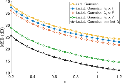
Figure 1: Gaussian mechanism - MSE vs. $\epsilon$ for $K=20$ and $\delta=10^{-6}$.

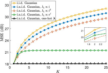
Figure 2: Gaussian mechanism - MSE vs. $K$ for $\epsilon=0.5$ and $\delta=10^{-6}$.

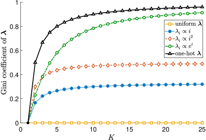
Figure 3: Gini coefficients of the sensitivity profiles.

Figure 4: Laplace mechanism - MSE vs. $\epsilon$ for $K=20\hskip 0.45003pt$.

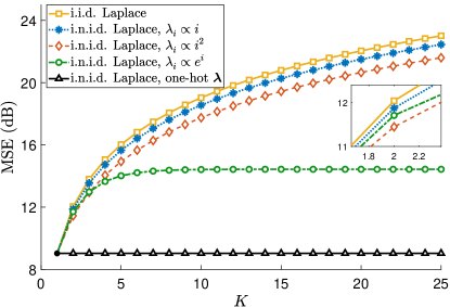
Figure 5: Laplace mechanism - MSE vs. $K$ for $\epsilon=0.5\hskip 0.45003pt$.

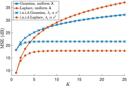
Figure 6: Comparison of Gaussian and Laplace mechanisms with varying $K$.

The performance of i.n.i.d. Gaussian mechanism with varying dimension $K$ is studied next. The MSE curves for different $K$ are given in Figure 2 for the privacy parameters $\epsilon=0.5$ and $\delta=10^{-6}\hskip 0.50003pt$. Figure 3 shows the Gini coefficients with varying $K$ for various sensitivity profiles. From Figure 2, we can observe that the MSE of i.n.i.d. mechanism pertaining to quadratic profile is better than that corresponding to linear profile, which in turn offers lesser MSE than uniform profile (which coincides with the MSE of i.i.d. mechanism). The exponential profile results in lesser MSE than the quadratic one for $K\geq 3$; for $K=2$ quadratic profile is better (please see the inset plot in Figure 2) because the quadratic profile is more spread out than the exponential one when $K=2\hskip 0.50003pt$, which is evident from the larger Gini coefficient of the quadratic profile in Figure 3. These results are in accordance with Theorem 7, that the most dispersed $\boldsymbol{{\lambda}}$ is associated with the least MSE.

It can also be observed that the reduction in MSE of the i.n.i.d. mechanism over i.i.d. one improves with $K$. However, for large $K$, the incremental reduction in MSE is smaller for the linear and quadratic profiles; for instance, both these profiles give only $0.02\hskip 1.00006pt\mathrm{dB}$ improvement for $K=25$ compared to $K=20\hskip 0.50003pt$. However, the exponential profile provides a substantial reduction in MSE with increasing $K$ compared to the i.i.d. mechanism. This is because the MSE for the i.i.d. case increases linearly with $K$, $\left\lVert\boldsymbol{\sigma}_{0}\right\rVert_{2}^{2}=\tfrac{K\Delta_{2}^{2}}{{M}_{0}^{2}}\hskip 0.50003pt$, whereas the MSE curve for the exponential profile saturates for large $K$ at $21.477\hskip 1.00006pt\mathrm{dB}\hskip 0.50003pt$.

V-B Laplace mechanism

The MSE curves of the i.n.i.d. Laplace mechanism that guarantees $\epsilon$-DP with varying $\epsilon$ is plotted in Figure 5 and Figure 5 shows the MSE with varying $K$. As with the Gaussian case, i.n.i.d. noise always provides improvement over the i.i.d. noise, and the reduction in MSE improves with the increase in the dispersion of $\boldsymbol{{\lambda}}\hskip 0.50003pt$. Particularly, in Figure 5, we can see that the i.n.i.d. Laplace noise reduces the MSE by $0.546\hskip 1.00006pt\mathrm{dB}\hskip 0.50003pt$, $1.39\hskip 1.00006pt\mathrm{dB}$ and $7.609\hskip 1.00006pt\mathrm{dB}$ consistently over all $\epsilon\hskip 0.50003pt$, for the linear, quadratic and exponential sensitivity profiles, respectively. Figure 5 also depicts a similar trend as that of our simulations for the Gaussian mechanism in Figure 2. The i.n.i.d. mechanism for the exponential profile offers lesser MSE than that pertaining to quadratic and linear profiles for larger $K$ and the reduction in MSE improves with $K$ since the MSE saturates at $14.243\hskip 1.00006pt\mathrm{dB}\hskip 0.50003pt$, which is $5.4\hskip 1.00006pt\mathrm{dB}$ above the MSE for one-hot $\boldsymbol{{\lambda}}\hskip 0.50003pt$.

V-C Comparison of Gaussian and Laplace mechanisms

Finally, in Figure 6, we compare the MSE pertaining to i.n.i.d. Laplace mechanism for $\epsilon=0.5$ with i.n.i.d. Gaussian mechanism for $\epsilon=0.5$ and $\delta=10^{-6}$ for different dimensions $K$. For this simulation, $\boldsymbol{{\lambda}}$ is normalized to have $\Delta_{2}=1\hskip 0.50003pt$. Although the Gaussian mechanism is unable to provide the stronger $\epsilon$-DP guarantee with $\delta=0\hskip 0.50003pt$, one of the reasons it is widely used is that it offers lesser MSE in higher dimensions than Laplace. This is the case for the uniform $\boldsymbol{\lambda}$ and we observe that the Laplace noise results in higher MSE than the Gaussian for $K\geq 9$ in Figure 6. However, when ${\lambda}_{i}\propto e^{i}$, the i.n.i.d. Laplace mechanism offers lesser MSE than the Gaussian for all dimensions, despite ensuring the stronger $\epsilon$-DP condition. Hence, the choice of noise distribution should not only be based on the dimension but also take into account the individual sensitivities.

VI Conclusions

We have introduced i.n.i.d. noise addition to perturb the query results on databases to guarantee privacy. In particular, Gaussian and Laplace i.n.i.d. mechanisms are studied in detail. The use of i.n.i.d. noise offers more degrees-of-freedom with one scale parameter per coordinate and the MSE can be minimized by exploiting the disparity in the sensitivities across the coordinates.

The appropriate choices for the scale parameters for the i.n.i.d. Gaussian and Laplace mechanisms that result in the lowest possible MSE for the required privacy guarantees have been derived. It has been shown theoretically and empirically that this choice of parameters improves the utility over the i.i.d. noise for a wide range of scenarios. We have also observed that the Laplace mechanism can result in lesser perturbation than Gaussian even in higher dimensions for certain cases when i.n.i.d. noise is added.

Appendix A Solving the optimization problem (P2)

To solve the problem (P2) efficiently, we make use of the monotonicity of the constraint function. Let us consider the function

$$J_{\epsilon,\delta}(w)={Q}\!\left({w\epsilon}-\tfrac{1}{2w}\right)\!\hskip 0.50003pt-e^{\epsilon}{Q}\!\left({w\epsilon}+\tfrac{1}{2w}\right)\!-\delta={\phi}_{\epsilon}\big{(}\tfrac{1}{w}\big{)}-\delta\hskip 0.50003pt.$$

Also, let $w_{0}$ be its (positive) root, $J_{\epsilon,\delta}(w_{0})=0$. we know that $\phi_{\epsilon}$ is a monotonic increasing function on $\mathbb{R}_{++}$ from Lemma 3, therefore, $J_{\epsilon,\delta}$ is a monotonic decreasing function on $\mathbb{R}_{++}\hskip 0.50003pt$. Hence, $w_{0}$ corresponds to the smallest $w$ so that ${\phi}_{\epsilon}\big{(}\tfrac{1}{w}\big{)}\leq\delta$ and the solution to the problem (P2) is given as $M_{0}=1/w_{0}\hskip 0.50003pt$; thus, we focus on obtaining the root $w_{0}$ of the function $J_{\epsilon,\delta}$ in the sequel.

Algorithm 1 Bisection method to solve (P2)

Input: privacy parameters $\epsilon\geq 0$ and $\delta\in[0,1]\hskip 0.50003pt$, tolerance level $w_{\texttt{tol}}$.

$[w_{l},w_{u}]\leftarrow\big{[}0\hskip 0.50003pt,\tfrac{1}{2\epsilon}\big{(}Q^{-1}(\delta)+\sqrt{(Q^{-1}(\delta))^{2}+2\epsilon}\big{)}\big{]}$.

repeat

     $w_{m}\leftarrow(w_{l}+w_{u})/2\hskip 0.50003pt$.

     if  $J_{\epsilon,\delta}(w_{m})>0$  then

         $w_{l}\leftarrow w_{m}$.

     else

         $w_{u}\leftarrow w_{m}$.

     end if

until $w_{u}-w_{l}\leq w_{\texttt{tol}}$.

$w_{0}=w_{u}$.

Output: $M_{0}=1/w_{0}$.

Since $J_{\epsilon,\delta}$ is monotonic decreasing, it is also quasi-concave and the root $w_{0}$ can be obtained using the bisection method [21], which is exponentially faster than other numerical methods. Bisection method is iterative. It begins with an interval in which the function $J_{\epsilon,\delta}$ changes its sign and in each iteration, it shrinks the interval to half its current length so that the function still changes the sign in the new interval. The procedure can be terminated once the length of the interval gets smaller than the required level of accuracy in the root.

We know that the function $J_{\epsilon,\delta}$ is bounded above by $J_{\epsilon,\delta}^{{}_{(u)}}$ given by

$$J_{\epsilon,\delta}^{{}_{(u)}}(w)={Q}\!\left({w\epsilon}-\tfrac{1}{2w}\right)\!-\delta\hskip 1.00006pt.$$

Note that $J_{\epsilon,\delta}^{{}_{(u)}}(w)$ is also monotonic decreasing; therefore, its root [7]

$$w_{0}^{{}_{(u)}}=\tfrac{1}{2\epsilon}\big{(}Q^{-1}(\delta)+\sqrt{(Q^{-1}(\delta))^{2}+2\epsilon}\hskip 0.50003pt\big{)}$$

is also above $w_{0}$ and we have $J_{\epsilon,\delta}(w_{0}^{{}_{(u)}})<0$. Also, we have $\lim\limits_{w\to 0}\,J_{\epsilon,\delta}(w)=1-\delta\geq 0\hskip 0.50003pt$. Thus, $J_{\epsilon,\delta}(w)$ changes its sign over $w\in[0,w_{0}^{{}_{(u)}}]\hskip 0.50003pt$. We can chose this interval as the initial interval for the bisection method for obtaining the root $w_{0}\hskip 0.50003pt$. Once the interval gets shorter than the tolerance level in the bisection method, we take $w_{0}$ as the upper limit of that interval since it holds that ${\phi}_{\epsilon}\big{(}\tfrac{1}{w_{u}}\big{)}\leq\delta\hskip 0.50003pt$, and the optimum of (P2) is computed as $M_{0}=1/w_{0}\hskip 0.50003pt$. The procedure is outlined in Algorithm 1.

References

• [1] C. Dwork, A. Roth et al., “The algorithmic foundations of differential privacy.” Foundations and Trends in Theoretical Computer Science, vol. 9, no. 3-4, pp. 211–407, 2014.
• [2] K. Chaudhuri, C. Monteleoni, and A. D. Sarwate, “Differentially private empirical risk minimization.” Journal of Machine Learning Research, vol. 12, no. 3, 2011.
• [3] N. Mohammed, R. Chen, B. C. Fung, and P. S. Yu, “Differentially private data release for data mining,” in Proceedings of the ACM SIGKDD international conference on Knowledge discovery and data mining, 2011, pp. 493–501.
• [4] S. Chien, P. Jain, W. Krichene, S. Rendle, S. Song, A. Thakurta, and L. Zhang, “Private alternating least squares: Practical private matrix completion with tighter rates,” in International Conference on Machine Learning.   PMLR, 2021, pp. 1877–1887.
• [5] M. Shechner, O. Sheffet, and U. Stemmer, “Private k-means clustering with stability assumptions,” in International Conference on Artificial Intelligence and Statistics.   PMLR, 2020, pp. 2518–2528.
• [6] C. Dwork, K. Kenthapadi, F. McSherry, I. Mironov, and M. Naor, “Our data, ourselves: Privacy via distributed noise generation,” in Annual international conference on the theory and applications of cryptographic techniques.   Springer, 2006, pp. 486–503.
• [7] J. Le Ny and G. J. Pappas, “Differentially private filtering,” IEEE Transactions on Automatic Control, vol. 59, no. 2, pp. 341–354, 2013.
• [8] B. Balle and Y.-X. Wang, “Improving the Gaussian mechanism for differential privacy: Analytical calibration and optimal denoising,” in International Conference on Machine Learning.   PMLR, 2018, pp. 394–403.
• [9] D. Desfontaines. (2020) The magic of Gaussian noise. [Online]. Available: https://desfontain.es/privacy/gaussian-noise.html
• [10] Y. Yang, P. Gohari, and U. Topcu, “Additive logistic mechanism for privacy-preserving self-supervised learning,” arXiv preprint arXiv:2205.12430, 2022.
• [11] S. A. Vinterbo, “Differential privacy for symmetric log-concave mechanisms,” in International Conference on Artificial Intelligence and Statistics.   PMLR, 2022, pp. 6270–6291.
• [12] F. Liu, “Generalized gaussian mechanism for differential privacy,” IEEE Transactions on Knowledge and Data Engineering, vol. 31, no. 4, pp. 747–756, 2018.
• [13] P. Sadeghi and M. Korki, “Offset-symmetric gaussians for differential privacy,” IEEE Transactions on Information Forensics and Security, vol. 17, pp. 2394–2409, 2022.
• [14] G. Muthukrishnan and S. Kalyani, “Grafting Laplace and Gaussian distributions: A new noise mechanism for differential privacy,” arXiv preprint arXiv:2212.09657, 2022.
• [15] I. Dinur and K. Nissim, “Revealing information while preserving privacy,” in Proceedings of the ACM SIGMOD-SIGACT-SIGART symposium on Principles of database systems, 2003, pp. 202–210.
• [16] B. Balle, G. Barthe, and M. Gaboardi, “Privacy profiles and amplification by subsampling,” Journal of Privacy and Confidentiality, vol. 10, no. 1, 2020.
• [17] M. Goldberg, “Equivalence constants for $l_{p}$ norms of matrices,” Linear and Multilinear Algebra, vol. 21, no. 2, pp. 173–179, 1987.
• [18] X. Tian and J. Taylor, “Selective inference with a randomized response,” The Annals of Statistics, vol. 46, no. 2, pp. 679–710, 2018.
• [19] C. Dwork, F. McSherry, K. Nissim, and A. Smith, “Calibrating noise to sensitivity in private data analysis,” in Theory of cryptography conference.   Springer, 2006, pp. 265–284.
• [20] R. V. Hogg and A. T. Craig, Introduction to Mathematical Statistics, 8th ed.   Pearson Education, Inc., 2019.
• [21] S. Boyd and L. Vandenberghe, Convex optimization.   Cambridge university press, 2004.
• [22] A. W. Marshall, I. Olkin, and B. C. Arnold, Inequalities: theory of majorization and its applications.   Springer, 2011.
• [23] G. H. Hardy, J. E. Littlewood, and G. Pólya, “Some simple inequalities satisfied by convex functions,” Messenger Math., vol. 58, pp. 145–152, 1929.