OPORP: One Permutation + One Random Projection

Abstract

OPORP is an improved variant of the count-sketch data structure by using a fixed-length binning scheme and a normalization step for the estimation. In our experience, we find engineers like the name “one permutation + one random projection” as it tells the exact steps.

Consider two data vectors (e.g., embeddings): $u,v\in\mathbb{R}^{D}$. In many embedding-based applications where vectors are generated from trained models, $D=256\sim 1024$ are common and $D>1024$ is not rare (e.g., GPT models). $D$ can be much larger in applications where the vectors are generated without training. With OPORP, we first apply a permutation on the data vectors. A random vector $r\in\mathbb{R}^{D}$ is generated with moments: $E(r_{i})=0,E(r_{i}^{2})=1,E(r_{i}^{3})=0,E(r_{i}^{4})=s$. Note that $s=3$ if $r_{i}$ follows the standard Gaussian distribution. We multiply $r$ (element-wise) with all permuted data vectors. Then we break the $D$ columns into $k$ equal-length bins and aggregate (i.e., sum) the values in each bin to obtain $k$ samples from each data vector. One key step is to normalize the $k$ samples to the unit $l_{2}$ norm. In this way, for the two original data vectors $u,v\in\mathbb{R}^{D}$, we obtain two new vectors $x,y\in\mathbb{R}^{D}$ with unit $l_{2}$ norms. The inner product of $x,y$ approximates the original correlation $\rho$ (i.e., the cosine) between $u$ and $v$. Our main contribution is to show that the estimation variance has essentially the following expression:

$$(s-1)A+\frac{D-k}{D-1}\frac{1}{k}\left[(1-\rho^{2})^{2}-2A\right],\hskip 14.45377pt\text{where }\ s\geq 1\ ,\ A\geq 0.$$

This variance formula reveals several key properties of the proposed scheme and estimator:

• We need $s=1$, otherwise the variance has a term which does not decrease with increasing sample size $k$. There is only one such distribution: $r_{i}\in\{-1,+1\}$ with equal probabilities.

• The factor $\frac{D-k}{D-1}$ can be quite beneficial in reducing variances. When $k=D$, the variance is zero. When $k=D/2$ (and $s=1$), the variance is reduced by $50\%$. When $k=D/4$ (which is also a common practical situation), the variance is reduced by $25\%$.

• The term $(1-\rho^{2})^{2}$ represents another (drastic) variance reduction due to normalization, compared to $(1+\rho^{2})$, which is the corresponding term without normalization. Interestingly, $(1-\rho^{2})^{2}$ also matches the classical asymptotic variance of the classical correlation estimator.

The OPORP procedure can be repeated $m$ times to improve the estimate. We illustrate that, by letting the $k$ in OPORP to be $k=1$ and repeat the procedure $m$ times, we exactly recover the work of “very sparse random projections” (VSRP) (Li et al., 2006b). This immediately leads to a normalized estimator for VSRP which substantially improves the original estimator of VSRP.

In summary, the two key steps in OPORP: (i) normalization and (ii) fixed-length binning, have considerably improved the accuracy in estimating the cosine similarity, which is a routine (and crucial) task in modern embedding-based retrieval (EBR) applications. Count-sketch type of data structures have been widely used in feature hashing for AI model compression, heavy-hitter detection, efficient communication in federated learning, and privacy (Li and Li, 2023).

1 Introduction

Given two $D$-dimensional vectors, $u,v\in\mathbb{R}^{D}$, a common task is to compute the “cosine” similarity:

$$\rho=\frac{\sum_{i=1}^{D}u_{i}v_{i}}{\sqrt{\sum_{i=1}^{D}u_{i}^{2}}\sqrt{\sum_{i=1}^{D}v_{i}^{2}}}.$$ (1)

Some applications also need to compute the inner product $a$ and the $l_{2}$ distance $d$:

$$a=\sum_{i=1}^{D}u_{i}v_{i},\hskip 28.90755ptd=\sum_{i=1}^{D}|u_{i}-v_{i}|^{2}.$$ (2)

The data vectors can be the “embeddings” learned from deep learning models such as the celebrated “two-tower” model (Huang et al., 2013). They can also be data vectors processed without training, for example, the $n$-grams (shingles), which can be extremely high-dimensional, e.g., $D$ is million or billion or even higher depending on the choice of “$n$” in $n$-grams (Broder, 1997; Broder et al., 1997; Li and Church, 2005; Das et al., 2007; Chierichetti et al., 2009; Li et al., 2008, 2012; Tamersoy et al., 2014; Nargesian et al., 2018; Wang et al., 2019; Li and Li, 2022).

It is often the case that the embedding vectors generated from deep learning models are relatively short (e.g., $D=256$ or $D=1024$), often dense, and typically normalized, i.e., $\sum_{i=1}^{D}u_{i}^{2}=\sum_{i=1}^{D}v_{i}^{2}=1$. (In this study, we will not assume the original data vectors are normalized.) For example, for BERT-type of embeddings (Devlin et al., 2019), the embedding size $D$ is typically 768 or 1024; and Applications with BERT models may also use higher embedding dimensions, e.g., $D=4096$ (Giorgi et al., 2021). For GLOVE word embeddings (Pennington et al., 2014), $D=300$ is often the default choice. In recent EBR (embedding based retrieval) applications (Chang et al., 2020; Yu et al., 2022b, a), using $D=256$ or $D=512$ appears common. For knowledge graph embeddings, we see the use of embedding size $D=256\sim 768$ (Huang et al., 2019; Spillo et al., 2022). In many computer vision applications, the embedding sizes are often larger, e.g., 4096, 8192 or even larger (Karpathy et al., 2014; Yu et al., 2018; Lanchantin et al., 2021). The recent advances in GPT-3 models (Brown et al., 2020) for NLP tasks (text classification, semantic search, etc.) learn word embeddings with $D=1024\sim 12288$ (Neelakantan et al., 2022).

In practical scenarios, the cost for storing the embeddings is usually expensive. In fact, even with merely $D=256$, the storage cost for the embeddings can be prohibitive in industrial applications. For example, suppose an app has 100 million (active) users and each user is represented by a $D=256$ embedding vector. Then storing the embeddings (assuming each dimension is a 4-byte real number) would cost 100GB. It will make the deployment much easier if the storage can be reduced to, say 25GB (a 4-fold reduction) or 12.5GB (a 8-fold reduction). Reducing the embedding size will, of course, also translate into the reductions in the computational and communication costs.

In this paper, we study a compression scheme based on the idea of “one permutation + one random projection”, or OPORP for short. It basically uses the (variant of) count-sketch data structure (Charikar et al., 2004), with several differences: (i) we focus on one permutation and one random projection (while it is straightforward to extend the analysis to multiple projections); (ii) we use a fixed-length binning scheme; (iii) we adopt a normalization step in the estimation stage. Compared with the previous works (Weinberger et al., 2009; Li et al., 2011) which used count-sketch type data structures for building large-scale machine learning models, the normalization step very significantly reduces the estimation variance, as shown by our theoretical analysis. In addition, the fixed-binning scheme brings in a multiplicative term $\frac{D-k}{D-1}$ in the variance which also substantially reduces the estimation error when $k=D/2$ (i.e., a 50% variance reduction) or even just $k=D/4$.

1.1 Count-Sketch and Variants

We briefly review the count-sketch data structure (Charikar et al., 2004). Count-sketch first uses a hash function $h:[D]\mapsto[k]$ to uniformly map each data coordinate to one of $k$ bins, and then aggregates the coordinate values within the bin. Here, each coordinate $i\in[1,D]$ is further multiplied by a Rademacher variable $r_{i}$ with $P(r_{i}=-1)=P(r_{i}=1)=1/2$. The binning procedure of count-sketch can be interpreted, in a probabilistically equivalent manner, as the “variable-length binning scheme”. That is, we first apply a random permutation on the data vector and splits the coordinates into $k$ bins whose lengths follow a multinomial distribution. Also, in the original count-sketch, the above procedure is repeated $m$ times (for identifying heavy hitters, another term for “compressed sensing”). The count-sketch data structure and variants have been widely used in applications. Recent examples include graph embedding (Wu et al., 2019), word & image embedding (Chen et al., 2017; Zhang et al., 2020; AlOmar et al., 2021; Singhal et al., 2021; Zhang et al., 2022), model & communication compression (Weinberger et al., 2009; Li et al., 2011; Chen et al., 2015; Rothchild et al., 2020; Haddadpour et al., 2020), etc. Note that in many applications, only $m=1$ repetition is used. Our study will focus on $m=1$ and the analysis can be extended to $m>1$. In fact, we can recover “very sparse random projections” (VSRP) (Li et al., 2006b) if we let $m>1$ (and $k=1$, i.e., using just one bin for each repetition). This is an interesting insight/connection.

1.2 Random Projections (RP) and Very Sparse Random Projections (VSRP)

To a large extent, the work of OPORP is also closely related to random projections (RP), especially the “sparse” or “very sparse” random projections (Achlioptas, 2003; Li et al., 2006b). The basic idea of random projections is to multiply the original data vectors, e.g., $u\in\mathbb{R}^{D}$ with a random matrix $R\in\mathbb{R}^{D\times k}$ to generate new vectors, e.g., $x\in\mathbb{R}^{k}$, as samples from which we can recover the original similarities (e.g., the inner products or cosines). The entries of the random matrix $R$ are typically sampled i.i.d. from the standard Gaussian distribution or the Rademacher distribution. The projection matrix can also be made (very) sparse to facilitate the computation. For instance, the entries in $R$ take values in $\{-1,0,1\}$ with probabilities $\{1/(2s),1-1/s,1/(2s)\}$, and we can control the sparsity by altering $s$. In many cases, $R$ can be considerably sparse while maintaining good learning capacity/utility. For example, in our experiments (Section 4), the learning performance does not drop much when the projection matrix contains around 90% zeros (i.e., $s=10$) on average.

As an effective tool for dimensionality reduction and geometry preservation, the methods of (very sparse) random projections have been widely adopted by numerous applications in data mining, machine learning, computational biology, databases, compressed sensing, etc. (Johnson and Lindenstrauss, 1984; Goemans and Williamson, 1995; Dasgupta, 2000; Bingham and Mannila, 2001; Buhler, 2001; Charikar, 2002; Fern and Brodley, 2003; Achlioptas, 2003; Datar et al., 2004; Candès et al., 2006; Donoho, 2006; Li et al., 2006b; Rahimi and Recht, 2007; Dasgupta and Freund, 2008; Li et al., 2014; Li and Li, 2019b, a; Rabanser et al., 2019; Tomita et al., 2020; Li and Li, 2021).

1.3 OPORP versus VSRP

We will demonstrate that we can utilize OPORP to recover “very sparser random projections” (VSRP) (Li et al., 2006b). Basically, we have the option of repeating the OPORP procedure $m$ times, which will reduce the variance while increasing the sample size. Interestingly, by using $m$ repetitions and letting the $k$ (number of bins) in OPORP to be $k=1$, we exactly recover VSRP with $m$ projections. This means that the theory we develop for OPORP also applies to VSRP. In particular, we immediately obtain the normalized estimator for VSRP and its theoretical variance. Therefore, OPORP and VSRP are the two extreme examples of the family of (sparse) random projections. In this paper, we show that with merely $m=1$ repetition, OPORP has already achieved smaller variances than the standard random projections and very sparse random projections. If we hope to achieve the same level of sparsity of the projection matrix, OPORP could be substantially more accurate than VSRP (depending on data distributions).

2 The Proposed Algorithm of OPORP

As the name “OPORP” suggests, the proposed algorithm mainly consists of applying “one permutation” then “one random projection” on the data vectors $\in\mathbb{R}^{D}$, for the purpose of reducing the dimensionality, the memory/disk space, and the computational cost. The dimensionality $D$ varies significantly, depending on applications. As discussed in the Introduction, for embedding vectors generated from learning models, using $D=256\sim 1024$ is fairly common although some applications use $D=8192$ or even larger. As long as the embedding size $D$ is not too large, it is affordable (and convenient) to simply generate and store the permutation vector and the random projection vector. In fact, even when $D$ is as large as a billion ($D=10^{9}$), storing two $10^{9}$-dimensional dense vectors is often affordable. On the other hand, for applications which need $D\gg 10^{9}$, we might have to resort to various approximations to generate the permutation/projection vectors such as the standard “universal hashing” (Carter and Wegman, 1977). In particular, in the literature of ($b$-bit) minwise hashing and related techniques (Broder, 1997; Broder et al., 1997, 1998; Indyk, 1999; Charikar, 2002; Li et al., 2008, 2012; Shrivastava, 2016; Li and Li, 2022), there are abundance of discussions about generating (high quality) permutations in extremely high-dimensional space. In this paper, we will simplify the discussion by assuming a random permutation vector and a random projection vector.

2.1 The Procedure of OPORP

In summary, the procedure of OPORP has the following steps:

• Generate a permutation $\pi:[D]\longrightarrow[D]$.

• Apply the same permutation to all data vectors, e.g., $u,v\in\mathbb{R}^{D}$.

• Generate a random vector $r$ of size $D$, with i.i.d. entries $r_{i}$ of the following first four moments:

  $$E(r_{i})=0,\hskip 21.68121ptE(r_{i}^{2})=1,\hskip 21.68121ptE(r_{i}^{3})=0,\hskip 21.68121ptE(r_{i}^{4})=s.$$ (3)

  Our calculation will show that $s=1$ leads to the smallest variance of OPORP. There exists only one such distribution if we let $s=1$, that is, $r_{i}\in\{-1,1\}$ with equal probabilities, i.e., the Rademacher distribution. We carry out the calculations for general $s$, for the convenience of comparing with “very sparse random projections” (VSRP) (Li et al., 2006b). In fact, this will also develop the new theory and estimator for VSRP.

• Divide the $D$ columns into $k$ bins. There are two binning strategies:

  1. Fixed-length binning scheme: every bin has a length of $D/k$. We assume $D$ is divisible by $k$; if not, we can always pad zeros. In the practice of embedding-based retrieval (EBR), as it is often to let $D=2^{8}=256$ or $D=2^{10}=1024$, we can conveniently choose (e.g.,) $k=2^{6}=64$. Our analysis will show that using this fixed-length scheme will result in a variance reduction by a factor of $\frac{D-k}{D-1}$, which is quite significant for typical EBR applications, compared to the commonly analyzed variable-length binning scheme.

  2. Variable-length binning scheme: the bin lengths follow a multinomial distribution
     $multinomial(D,1/k,1/k,....,1/k)$ with $k$ bins. Note that $k$ can be larger than $D$, i.e., some bins will be empty. When $k\rightarrow\infty$, it essentially recovers the fixed-length binning scheme with $k=D$. The variable-length binning scheme is the strategy in the previous literature (Charikar et al., 2004; Weinberger et al., 2009; Li et al., 2011).

• For each bin and each data vector, we generate a sample as follows:

  $$x_{j}=\sum_{i=1}^{D}u_{i}r_{i}I_{ij},\hskip 21.68121pty_{j}=\sum_{i=1}^{D}v_{i}r_{i}I_{ij},\hskip 14.45377ptj=1,2,...,k$$ (4)

  where $I_{ij}$ is an indicator: $I_{ij}=1$ if the original coordinate $i$ is mapped to bin $j$, and $I_{ij}=0$ otherwise. Because there are two binning schemes, wherever necessary, we will use $I_{1,ij}$ (fixed-length) and $I_{2,ij}$ (variable-length) to differentiate these two binning schemes.

After we have obtained the samples (e.g., $x_{j}$, $y_{j}$), we can estimate the inner product $a$, the $l_{2}$ distance $d$, and the cosine $\rho$ of the original data vectors, as follows:

$$\hat{a}=\sum_{j=1}^{k}x_{j}y_{j},\hskip 14.45377pt\hat{d}=\sum_{j=1}^{k}|x_{j}-y_{j}|^{2},\hskip 14.45377pt\hat{\rho}=\frac{\sum_{j=1}^{k}x_{j}y_{j}}{\sqrt{\sum_{j=1}^{k}x_{j}^{2}}\sqrt{\sum_{j=1}^{k}y_{j}^{2}}}.$$ (5)

Note that, for the estimator $\hat{\rho}$, the normalization step is not needed at the estimation time if we pre-normalize and store the data, e.g., $x_{j}^{\prime}=\frac{x_{j}^{\prime}}{\sqrt{\sum_{t=1}^{k}x_{t}^{2}}}$. This is a notable advantage. Also, wherever necessary, we will again use $\hat{a}_{1}$, $\hat{a}_{2}$, $\hat{d}_{1}$, $\hat{d}_{2}$, $\hat{\rho}_{1}$, $\hat{\rho}_{2}$, to differentiate the two binning schemes. We should mention that we will not assume the original data vectors are normalized to the unit $l_{2}$ norms, although in the practice of embedding-based retrieval (EBR), the embedding vectors are typically normalized.

If the original data vectors ($u$, $v$) are normalized, then $\hat{a}$ also provides an estimate of the original cosine because the original inner product is identical to the cosine in normalized data. One of the main contributions in this paper is to show that using $\hat{\rho}$ would be substantially more accurate than using $\hat{a}$ even when the original data are already normalized. Basically, the estimation variance of $\hat{\rho}$ is proportional to $(1-\rho^{2})^{2}$ while the estimation of $\hat{a}$ (in normalized data) is proportional to $1+\rho^{2}$. The difference between $(1-\rho^{2})^{2}$ and $1+\rho^{2}$ can be highly substantial, especially for $|\rho|$ close to 1.

2.2 The Choice of $r$

For the random projection vector $r\in\mathbb{R}^{D}$, we have only specified that its entries are i.i.d. and obey the following moment conditions:

$$E(r_{i})=0,\hskip 21.68121ptE(r_{i}^{2})=1,\hskip 21.68121ptE(r_{i}^{3})=0,\hskip 21.68121ptE(r_{i}^{4})=s,\hskip 7.22743pts\geq 1.$$

Note that $s\geq 1$ is needed because $E(r_{i}^{4})\geq E^{2}(r_{i}^{2})=1$ (the Cauchy-Schwarz Inequality). Typically, users who are familiar with random projections might attempt to sample $r$ from the Gaussian distribution. Our analysis, however, will show that the Gaussian distribution should not be used for OPORP. This is quite different from the standard random projections for which using either the Gaussian distribution or the Rademacher distribution (i.e., $r_{i}\in\{-1,+1\}$ with equal probabilities) would not make an essential difference. For OPORP, our analysis will show that we should use $s=1$ (i.e., the Rademacher distribution), by carrying out the calculations for general $s\geq 1$.

Here, we list some common distributions, which satisfy the moment conditions, as follows:

• The standard Gaussian distribution $N(0,1)$. This is the popular choice in the literature of random projections. The fourth moment of the standard Gaussian is 3, i.e., $s=3$.

• The uniform distribution, $\sqrt{3}\times unif[-1,1]$. We need the $\sqrt{3}$ factor in order to have $E(r_{i}^{2})=1$. For this choice of distribution, we have $E(r_{i}^{4})=s=9/5$.

• The “very sparse” distribution, as used in Li et al. (2006b):

  $$r_{i}=\sqrt{s}\times\left\{\begin{array}[]{rrl}-1&\text{with prob.}&1/(2s)\\ 0&\text{with prob.}&1-1/s\\ +1&\text{with prob.}&1/(2s)\end{array}\right.$$ (9)

  which generalizes Achlioptas (2003) (for $s=1$ and $s=3$).

2.3 Comparison with Very Sparse Random Projections (VSRP)

Note that for OPORP, even though it only effectively uses just one random projection, we can still view that as a random projection “matrix” $\in\mathbb{R}^{D\times k}$ with exactly one 1 on each row. In comparison, the “very sparse random projections” (VSRP) (Li et al., 2006b) uses a random projection matrix $\in\mathbb{R}^{D\times k}$ with entries sampled i.i.d. from the “very sparse” distribution (9). Interestingly, for VSRP, if we let its “$s$” parameter to be $s=k$, then OPORP (with its $s=1$) and VSRP will have the same sparsity on average in the projection “matrix”. In terms of the implementation, suppose we store the projection matrix, then it would be much more convenient to store the one projection vector for OPORP because it is really just a vector of length $D$. In comparison, storing the sparse random projection matrix would incur an additional overhead because we will have to store the locations (coordinates) of each non-zero entries. Thus, OPORP would be much more convenient to use.

In terms of the estimation variance, OPORP (with $s=1$) would be more accurate than VSRP, for several reasons. Firstly, OPORP with the fixed-length binning scheme has the $\frac{D-k}{D-1}$ variance reduction term, as will be shown in our theoretical analysis. Secondly, if we do not consider the $\frac{D-k}{D-1}$ term and we choose $s=1$ for both OPORP and VSRP, then their theoretical variances are identical for the un-normalized estimators. As long as $s>1$ for VSRP, the theoretical variance is larger than that of OPORP (for $s=1$). If we choose $s=k$ for VSRP (to achieve the same average sparsity as OPORP), then its variance might be significantly much larger, depending on the original data (e.g., $u$ and $v$). In addition, in this paper, we derive the variance formula for the normalized estimator of OPORP, which substantially improves the un-normalized estimator.

Finally, we should mention that we can actually recover VSRP if we just use one bin for OPORP and repeat the procedure $k$ times. This means that theory and estimators we develop for OPORP can be directly utilized to develop new theory and new estimator for VSRP. In particular, the normalized estimator for VSRP is developed whose variance can be directly inferred from OPORP.

In summary, OPORP and VSRP can be viewed as the two extreme examples of a family of sparse random projections. OPORP is more convenient to use and can be substantially more accurate than VSRP especially if we hope to maintain the same level of sparsity for the projection matrix.

3 Theoretical Analysis of OPORP and Numerical Verification

In this section, we conduct the theoretical analysis to derive the estimation variances for OPORP. Recall that, we generate $k$ samples as follows

$$x_{j}=\sum_{i=1}^{D}u_{i}r_{i}I_{ij},\hskip 21.68121pty_{j}=\sum_{i=1}^{D}v_{i}r_{i}I_{ij},\hskip 14.45377ptj=1,2,...,k$$

where $I_{ij}$ is a random variable determined by one of the following two binning schemes:

1. (First binning scheme) Fixed-length binning scheme: every bin has a length of $D/k$. We assume that $D$ is divisible by $k$, if not, we can always pad zeros.

2. (Second binning scheme) Variable-length binning scheme: the bin lengths follow a multinomial distribution $multinomial(D,1/k,1/k,....,1/k)$ with $k$ bins.

Specifically, $I_{ij}=1$ if the original coordinate $i\in[1,D]$ is mapped to bin $j\in[1,k]$; $I_{ij}=0$ otherwise. Wherever necessary, we will use $I_{1,ij}$ and $I_{2,ij}$ to differentiate the two binning schemes.

Lemma 1.

$\forall i\in[1,D]$, $j\in[1,k]$, $i\neq i^{\prime}$, $j\neq j^{\prime}$,

$$E(I_{1,ij})=E(I_{1,ij}^{n})=\frac{1}{k},n=1,2,3,...$$

$$E(I_{1,ij}I_{1,ij^{\prime}})=0,$$

$$E(I_{1,ij}I_{1,i^{\prime}j^{\prime}})=\frac{D}{D-1}\frac{1}{k^{2}},$$

$$E(I_{1,ij}I_{1,i^{\prime}j})=\frac{D-k}{D-1}\frac{1}{k^{2}},$$

$$E(I_{2,ij})=E(I_{2,ij}^{n})=\frac{1}{k},n=1,2,3,...$$

$$E(I_{2,ij}I_{2,ij^{\prime}})=0,$$

$$E(I_{2,ij}I_{2,i^{\prime}j^{\prime}})=\frac{1}{k^{2}},$$

$$E(I_{2,ij}I_{2,i^{\prime}j})=\frac{1}{k^{2}},$$

$$kE\left(I_{ij}I_{i^{\prime}j}\right)+k(k-1)E\left(I_{ij}I_{i^{\prime}j^{\prime}}\right)=1,$$

Proof of Lemma 1: Consider the first binning scheme, where all $k$ bins have the same length $D/k$. Thus, $E(I^{n}_{1,ij})=E(I_{1,ij})=\frac{D/k}{D}=\frac{1}{k}$. Each coordinate $i$ can only be mapped to one bin, hence $E(I_{1,ij}I_{1,ij^{\prime}})=0,\forall j\neq j^{\prime}$. To understand $E(I_{1,ij}I_{1,i^{\prime}j^{\prime}})=\frac{1}{k}\frac{D/k}{D-1}=\frac{D}{D-1}\frac{1}{k^{2}}$, we first assign $i$ to $j$ which occurs with probability $1/k$; then assign $i^{\prime}$ to $j^{\prime}$, which occurs with probability $\frac{D/k}{D-1}$ because the bin length is $D/k$ and there are $D-1$ locations left (as one is taken). Finally, to understand $E(I_{1,ij}I_{1,i^{\prime}j})=\frac{1}{k}\frac{D/k-1}{D-1}=\frac{D-k}{D-1}\frac{1}{k^{2}}$, we only have $D/k-1$ (instead of $D/k$) choices because one location in bin $j$ is already taken.

Next, we consider the second binning scheme. As the $k$ bin lengths follow the multinomial distribution, the results follow using properties of multinomial moments after some algebra. $\hfill\qed$

3.1 The Un-normalized Estimators

Once we have samples $x_{j}$, $y_{j}$, we can estimate the original inner product $a$ by $\hat{a}=\sum_{j=1}^{k}x_{j}y_{j}$. The results in Lemma 1 can assist us to derive the variances of the inner product estimators, $\hat{a}_{1}$ and $\hat{a}_{2}$ for two binning schemes, respectively.

Theorem 2.

$$E(\hat{a})=a,$$

$$Var(\hat{a}_{1})=\left(s-1\right)\sum_{i=1}^{D}u_{i}^{2}v_{i}^{2}+\frac{1}{k}\left(a^{2}+\sum_{i=1}^{D}u_{i}^{2}\sum_{i=1}^{D}v_{i}^{2}-2\sum_{i=1}^{D}u_{i}^{2}v_{i}^{2}\right)\frac{D-k}{D-1},$$

$$Var(\hat{a}_{2})=\left(s-1\right)\sum_{i=1}^{D}u_{i}^{2}v_{i}^{2}+\frac{1}{k}\left(a^{2}+\sum_{i=1}^{D}u_{i}^{2}\sum_{i=1}^{D}v_{i}^{2}-2\sum_{i=1}^{D}u_{i}^{2}v_{i}^{2}\right).$$

Proof of Theorem 2: See Appendix A. $\hfill\qed$

Compared to $Var(\hat{a}_{2})$ for the variable-bin-length scheme (which appeared in the prior work (Li et al., 2011)), the additional factor $\frac{D-k}{D-1}$ in $Var(\hat{a}_{1})$ demonstrates the benefit of the proposed fixed-bin-length strategy. Also, it is clear that we should choose $s=1$. What if we only use one bin, i.e., $k=1$? In this case $\frac{D-k}{D-1}=1$, i.e., two binning scheme becomes identical. This is of course expected and also explains why in $\frac{D-k}{D-1}$ we have $D-1$ instead of just $D$.

What will happen if we repeat OPORP $m$ times? In that case, the variances will be reduced by a factor of $\frac{1}{m}$, i.e.,

$$Var(\hat{a}_{1};m\text{ repetitions})=\frac{1}{m}\left[\left(s-1\right)\sum_{i=1}^{D}u_{i}^{2}v_{i}^{2}+\frac{1}{k}\left(a^{2}+\sum_{i=1}^{D}u_{i}^{2}\sum_{i=1}^{D}v_{i}^{2}-2\sum_{i=1}^{D}u_{i}^{2}v_{i}^{2}\right)\frac{D-k}{D-1}\right],$$

$$Var(\hat{a}_{2};m\text{ repetitions})=\frac{1}{m}\left[\left(s-1\right)\sum_{i=1}^{D}u_{i}^{2}v_{i}^{2}+\frac{1}{k}\left(a^{2}+\sum_{i=1}^{D}u_{i}^{2}\sum_{i=1}^{D}v_{i}^{2}-2\sum_{i=1}^{D}u_{i}^{2}v_{i}^{2}\right)\right].$$

Furthermore, if we let $k=1$ and still repeat $m$ times, then the two estimators become the same one and the variance would be

$$Var(\hat{a};m\text{ repetitions and }k=1)=\frac{1}{m}\left(a^{2}+\sum_{i=1}^{D}u_{i}^{2}\sum_{i=1}^{D}v_{i}^{2}+(s-3)\sum_{i=1}^{D}u_{i}^{2}v_{i}^{2}\right),$$

which is exactly the variance formula for the inner product estimator of “very sparse random projections” (VSRP) (Li et al., 2006b). In retrospect, this is expected because with $k=1$ for OPORP and $m$ repetitions, we recover the regular random projections with a projection matrix of size $D\times m$. We can also change the notation from $D\times m$ to $D\times k$ if the latter is more familiar to readers.

Once we have the variances for the inner products, it is straightforward to derive the variances for the distance estimators. To see this,

$$\hat{d}=\sum_{j=1}^{k}|x_{j}-y_{j}|^{2}=\sum_{j=1}^{k}\left|\sum_{i=1}^{D}u_{i}r_{i}I_{ij}-\sum_{i=1}^{D}v_{i}r_{i}I_{ij}\right|^{2}=\sum_{j=1}^{k}\left|\sum_{i=1}^{D}(u_{i}-v_{i})r_{i}I_{ij}\right|^{2}.$$

Clearly, we just need to replace, in Theorem 2, both $u_{i}$ and $v_{i}$ by $u_{i}-v_{i}$, in order to derive Theorem 3.

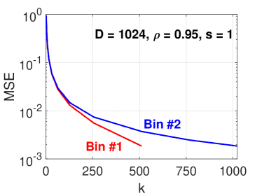
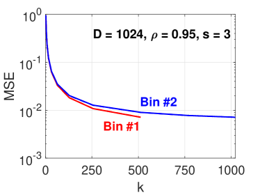
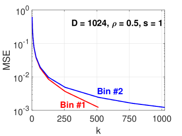
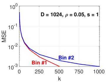
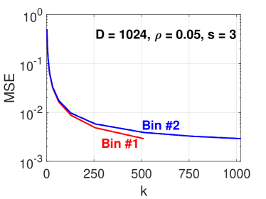
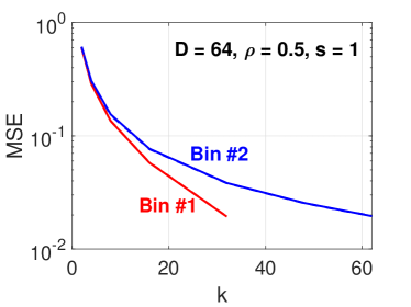
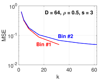
Figure 1: In each panel, we simulated two (normalized) vectors with the target $\rho$ value. Then we conduct OPORP $10^{5}$ times for each $k$, and both binning schemes. In each panel, the two solid curves represent the empirical mean square errors (MSE) and the two dashed curves for the theoretical variances. The dashed curves are not visible because they overlap with the solid curves. Note that for the fixed-length binning scheme (“Bin #1”), we cannot choose a $k$ in between $D/2$ and $D$.

Theorem 3.

$$E(\hat{d})=d,$$

$$Var(\hat{d}_{1})=\left(s-1\right)\sum_{i=1}^{D}|u_{i}-v_{i}|^{4}+\frac{1}{k}\left(2d^{2}-2\sum_{i=1}^{D}|u_{i}-v_{i}|^{4}\right)\frac{D-k}{D-1},$$

$$Var(\hat{d}_{2})=\left(s-1\right)\sum_{i=1}^{D}|u_{i}-v_{i}|^{4}+\frac{1}{k}\left(2d^{2}-2\sum_{i=1}^{D}|u_{i}-v_{i}|^{4}\right).$$

In the variance formulas, the term $\frac{D-k}{D-1}$ of the fixed-length binning scheme, would be very beneficial if $k$ is a considerable fraction of $D$. This is possible in EBR (embedding-based retrieval) applications where $D=256\sim 1024$ is typical. For example, when $D=256$ and $k=64$, we have $\frac{D-k}{D}=0.75$. A variance reduction by $25\%$ would be quite considerable especially as the fixed-length binning scheme is actually easier to implement than the variable-length binning scheme. The “only disadvantage” of the fixed-length scheme is that we cannot choose a $k$ value between $D/2$ and $D$.

Here, we provide a simulation study to verify Theorem 2 and present the simulation results in Figure 1. For each panel (for a specific target $\rho$) of Figure 1, we first generate two vectors from the standard bivariate Gaussian distribution with the target correlation $\rho$. To avoid ambiguity, we generate the vectors many times until we have two vectors whose cosine value is very close to the target $\rho$ before we store the vectors. Otherwise the empirical cosine value can be quite different from the target $\rho$. After we generate the two vectors, we normalize them to simplify the presentation of the results because otherwise the results would be related to the norms too. Then we conduct OPORP $10^{5}$ times for each $k$ in $\{2,4,8,16,32,...,D/2\}$. For convenience, we choose $D$ to be powers of 2. We only present results for $D=1024$ and $D=64$ because the other plots are pretty similar. Note that for the variable-length binning scheme, we also add simulations for $D/2<k<D$.

We report the simulations for both $s=1$ and $s=3$. In each panel, we plot four curves: the empirical mean square errors (MSE = variance + bias²) for both binning schemes, and the theoretical variance curves (in dashed lines) for both binning schemes. The dashed lines are not visible because they overlap with the empirical MSEs, which verify that the correctness of the variance formulas. We can also see that, with the fixed-length binning scheme (Bin#1), the variance is noticeably smaller than the variance of the variable-length scheme at the same $k$, confirming the benefits due to the $\frac{D-k}{D-1}$ term. Note that for $s=3$, the difference between the two binning scheme becomes smaller, because in the formulas the $\frac{D-k}{D-1}$ term does not apply to the term involving $(s-1)$.

3.2 The Normalized Estimators

One can (substantially) improve the estimation accuracy via the “normalization” trick. That is, once we have the samples ($x_{j}$, $y_{j}$), $j=1,2,...,k$, we can use the following normalized estimator:

$$\hat{\rho}=\frac{\sum_{j=1}^{k}x_{j}y_{j}}{\sqrt{\sum_{j=1}^{k}x_{j}^{2}}{\sqrt{\sum_{j=1}^{k}y_{j}^{2}}}}.$$

Again, we use $\hat{\rho}_{1}$ and $\hat{\rho}_{2}$ to denote the estimates for the fixed-length binning and variable-length binning, respectively. As explained earlier, the normalization step will not be needed at the estimation time if we pre-normalize and store the data, e.g., $x_{j}^{\prime}=\frac{x_{j}^{\prime}}{\sqrt{\sum_{t=1}^{k}x_{t}^{2}}}$.

Theorem 4.

For large $k$, $\hat{\rho}$ converges to $\rho$, almost surely, with

$$Var(\hat{\rho}_{1})= (s-1)A+\left\{\frac{1}{k}\left[(1-\rho^{2})^{2}-2A\right]+O\left(\frac{1}{k^{2}}\right)\right\}\frac{D-k}{D-1},$$

$$Var(\hat{\rho}_{2})= (s-1)A+\left\{\frac{1}{k}\left[(1-\rho^{2})^{2}-2A\right]+O\left(\frac{1}{k^{2}}\right)\right\}.$$

where

$$A=\sum_{i=1}^{D}\left(u_{i}^{\prime}v_{i}^{\prime}-\rho/2({u_{i}^{\prime}}^{2}+{v_{i}^{\prime}}^{2})\right)^{2},\hskip 14.45377ptu_{i}^{\prime}=\frac{u_{i}}{\sqrt{\sum_{t=1}^{D}u_{t}^{2}}},\hskip 14.45377ptv_{i}^{\prime}=\frac{v_{i}}{\sqrt{\sum_{t=1}^{D}v_{t}^{2}}}.$$

Proof of Theorem 4: See Appendix B. $\hfill\qed$

The variance expressions in Theorem 4 hold for large $k$ (i.e., $k\rightarrow D$ for the fixed-length binning and $k\rightarrow\infty$ for the variable-length binning). Note that the term $\frac{1}{k}\left(1-\rho^{2}\right)^{2}$ inside the variances of $\hat{\rho}$ is exactly the classical asymptotic variance of the correlation estimator for the bivariate Gaussian distribution (Anderson, 2003). Because $A\geq 0$, we know that OPORP achieves smaller (asymptotic) variance than the classical estimator in statistics, even without considering the $\frac{D-k}{D-1}$ factor.

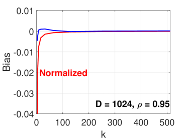
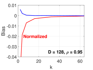
Figure 2: Empirical biases ($E\left(\hat{\rho}\right)-\rho$) of the normalized estimator $\hat{\rho}$ as well as the un-normalized estimator $\hat{a}$, evaluated on the same normalized data vectors in Figure 1, for $s=1$ and the fixed-length binning scheme. The empirical biases are very small (and bias² would be much smaller).

A simulation study presented in Figure 2 and Figure 3 shows that $k$ does not need to be large in order for these variance formulas to be sufficiently accurate.

In Figure 2 and Figure 3, we use the same data vectors as in Figure 1, for $s=1$ and only the fixed-length binning scheme. Recall that those generated vectors are already normalized, and hence the inner product is the same as the cosine. This makes it convenient to present both the un-normalized and normalized estimators in the same plot. Recall MSE = variance + bias². Figure 2 illustrates that the biases are very small (and bias² would be much smaller), as long as $k$ is not too small. The empirical MSE plots in Figure 3 confirms the significant variance reduction of the normalization step. The variance formula in Theorem 4 is accurate, as long as $k$ is not too small.

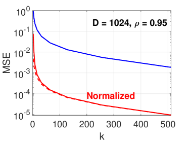
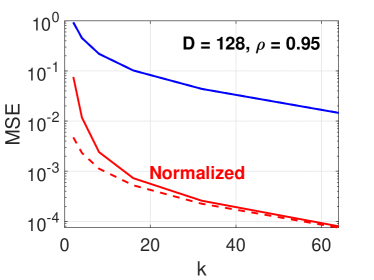
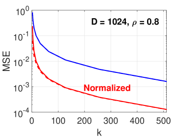
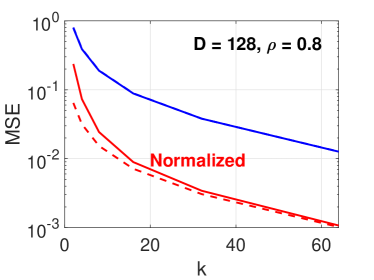
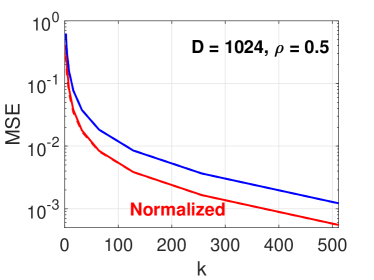
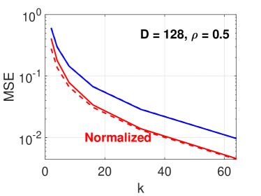
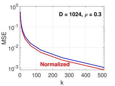
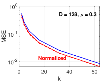
Figure 3: Empirical MSEs for both un-normalized and normalized estimators of OPORP, for $s=1$ and the fixed-length binning scheme, using the same normalized data vectors as in Figure 1. The normalization step reduces the MSEs considerably especially for large $\rho$ (i.e., more similar pairs). The dashed curves for the theoretical (asymptotic) variance of $\hat{\rho}$ in Theorem 4 differ slightly from the empirical MSEs (solid curves) if $k$ is small.

3.3 The Normalized Estimator for VSRP

We have already explained how to recover “very sparse random projections” (VSRP) (Li et al., 2006b) from OPORP by using $k=1$ and repeating OPORP $m$ times. We can therefore also take advantage of this finding to develop the normalized estimator for VSRP and obtain its variance. To present the estimator and its theory for VSRP, instead of introducing new notation, we borrow the existing notation. Also, we still use $k$ for the sample size of VSRP instead of $m$. That is, we have

$$x_{j}=\sum_{i=1}^{D}u_{i}r_{ij},\hskip 21.68121pty_{j}=\sum_{i=1}^{D}v_{i}r_{ij},\hskip 14.45377ptj=1,2,...,k.$$

where $r_{ij}$ follows the following sparse distribution parameterized by $s$:

$$r_{ij}=\sqrt{s}\times\left\{\begin{array}[]{rrl}-1&\text{with prob.}&1/(2s)\\ 0&\text{with prob.}&1-1/s\\ +1&\text{with prob.}&1/(2s)\end{array}\right.$$ (13)

We have the un-normalized estimator for $a$ and the normalized for $\rho$:

$$\hat{a}_{vsrp}=\frac{1}{k}\sum_{j=1}^{k}x_{j}y_{j},\hskip 14.45377pt\hat{\rho}_{vsrp}=\frac{\sum_{j=1}^{k}x_{j}y_{j}}{\sqrt{\sum_{j=1}^{k}x_{j}^{2}}{\sqrt{\sum_{j=1}^{k}y_{j}^{2}}}},$$

We have shown how to use the variance of $\hat{a}$ to recover the variance of $\hat{a}_{vsrp}$, as

$$Var(\hat{a}_{vsrp})=\frac{1}{k}\left(a^{2}+\sum_{i=1}^{D}u_{i}^{2}\sum_{i=1}^{D}v_{i}^{2}+(s-3)\sum_{i=1}^{D}u_{i}^{2}v_{i}^{2}\right).$$

As the normalized estimator and its variance for VSRP are new, we present the result as a theorem.

Theorem 5.

As $k\rightarrow\infty$, $\hat{\rho}_{vsrp}\rightarrow\rho$ almost surely, with

$$Var(\hat{\rho}_{vsrp})= \frac{1}{k}\left((1-\rho^{2})^{2}+(s-3)A\right)+O\left(\frac{1}{k^{2}}\right),$$

where

$$A=\sum_{i=1}^{D}\left(u_{i}^{\prime}v_{i}^{\prime}-\rho/2({u_{i}^{\prime}}^{2}+{v_{i}^{\prime}}^{2})\right)^{2},\hskip 14.45377ptu_{i}^{\prime}=\frac{u_{i}}{\sqrt{\sum_{t=1}^{D}u_{t}^{2}}},\hskip 14.45377ptv_{i}^{\prime}=\frac{v_{i}}{\sqrt{\sum_{t=1}^{D}v_{t}^{2}}}.$$

One way to compare VSRP (for general $s$) with OPORP (for $s=1$ and $m=1$ repetition), is to evaluate the following ratios of variances:

$$\frac{Var(\hat{a}_{vsrp,s})}{Var(\hat{a})}\approx\frac{\sum_{i=1}^{D}u_{i}^{2}\sum_{i=1}^{D}v_{i}^{2}+a^{2}+(s-3)\sum_{i=1}^{D}u_{i}^{2}v_{i}^{2}}{\sum_{i=1}^{D}u_{i}^{2}\sum_{i=1}^{D}v_{i}^{2}+a^{2}-2\sum_{i=1}^{D}u_{i}^{2}v_{i}^{2}},$$ (14)

$$\frac{Var(\hat{\rho}_{vsrp,s})}{Var(\hat{\rho})}\approx\frac{(1-\rho^{2})^{2}+(s-3)A}{(1-\rho^{2})^{2}-2A},$$ (15)

where we use $\approx$ as we neglect the beneficial factor of $\frac{D-k}{D-1}$ so that the comparison would favor VSRP. Obviously, when $s=1$, both ratios equal 1. The ratios increase with increasing $s$ for VSRP. Because the ratio is data-dependent, it is better that we compute it using real data.

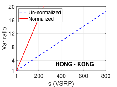
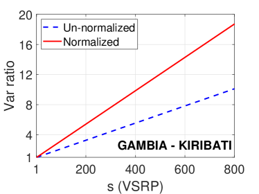
Figure 4: Ratio of variances in (14) and (15) to compare VSRP (parameterized by $s$) with OPORP (for its $s=1$), for both the un-normalized (dashed) and normalized (solid) estimators, on four selected word pairs from the “Words” dataset (see Table 1).

Table 1: Summary statistics of word-pairs from the “Words” dataset (Li and Church, 2005). For example, “HONG” represents a vector of length $2^{16}$ with each entry of the vector recording the number of documents that the “HONG” appears in the collection of $2^{16}$ documents.

word 1	word 2	$\rho$	$a=\sum_{i=1}^{D}u_{i}v_{i}$	$\sum_{i=1}^{D}u_{i}^{2}$	$\sum_{i=1}^{D}v_{i}^{2}$
HONG	KONG	0.9623	12967	13556	13395
WEEK	MONTH	0.8954	281297	323073	305468
OF	AND	0.8788	57219161	69006071	61437886
UNITED	STATES	0.6693	69201	85934	124415
BEFORE	AFTER	0.6633	59136	65541	121284
SAN	FRANCISCO	0.5623	29386	125109	21832
GAMBIA	KIRIBATI	0.5250	228	360	524
RIGHTS	RESERVED	0.3949	14710	79527	17449
HUMAN	NATURE	0.2992	14896	87356	28367

Figure 4 presents the variance ratios in (14) and (15) on four selected word (vector) pairs from the “Words” dataset; see Table 1 for the description of the data. In general, if the $s$ is not too large for VSRP (e.g., $s<10$), then VSRP works pretty well. For larger $s$, then the performance of VSRP largely depends on data. For example, on “SAN-FRANCISCO”, VSRP with the normalized estimator still works well (the variance ratio is smaller than 2) if with $s=200$. On “HONG-KONG”, however, VSRP does not perform well: for the normalized estimator, the variance ratio $>4$ when $s>40$; and for the un-normalized estimator, the variance ratio $>4$ when $s>150$.

The variance ratio = 4 means that we need to increase the sample size of VSRP by a factor of 4 in order to maintain the same accuracy. For VSRP with a the projection matrix size of size $D\times k$, it will need $s=k$ if we hope to achieve the same level of sparsity (on average) as OPORP. Depending on applications, we typically observe that $k=100\sim 500$ might be sufficient for the standard (dense) random projections. Therefore, VSRP using a large $s$ value may lead to poor performance in terms of the required number of projections (which is the also the sample size of VSRP).

In summary, VSRP should work well in general if we use a sparsity parameter $s$ around 10. VSRP may still perform well with a much larger $s$ but then that will be data-dependent. In Section 4, we will report the retrieval experimental results for VSRP, which also confirm the same finding.

3.4 The Inner Product Estimators

The simulations in Figure 1, Figure 2, and Figure 3 have used data vectors which are normalized to the unit $l_{2}$ norm, in part for the convenience of presenting the plots. In many EBR applications, the embedding vectors from learning models are indeed already normalized. On the other hand, there are also numerous applications which use un-normalized data. In fact, the entire literature about “maximum inner product search” (MIPS) (Ram and Gray, 2012; Shrivastava and Li, 2014; Bachrach et al., 2014; Tan et al., 2021) is built on the fact that in many applications the norms are different and the goal is to find the maximum inner products (instead of the cosines). Also see Fan et al. (2019) for the use of MIPS on advertisement retrievals in a commercial search engine.

Recall that, once we have the samples ($x_{j}$, $y_{j}$), $j=1,2,...,k$, we can estimate the inner product $a$ simply by $\hat{a}=\sum_{j=1}^{k}x_{j}y_{j}$. To improve the estimation accuracy, we can also utilize the normalized cosine estimator $\hat{\rho}=\frac{\sum_{j=1}^{k}x_{j}y_{j}}{\sqrt{\sum_{j=1}^{k}x_{j}^{2}}{\sqrt{\sum_{j=1}^{k}y_{j}^{2}}}}$ to have a “normalized inner product” estimator $\hat{a}_{n}$:

$$\hat{a}_{n}=\hat{\rho}\sqrt{\sum_{i=1}^{D}u_{i}^{2}}\sqrt{\sum_{i=1}^{D}v_{i}^{2}},$$

whose variance would be directly the scaled version of the variance of $\hat{\rho}$:

$$Var\left(\hat{a}_{n}\right)=Var\left(\hat{\rho}\right)\sum_{i=1}^{D}u_{i}^{2}\sum_{i=1}^{D}v_{i}^{2}.$$

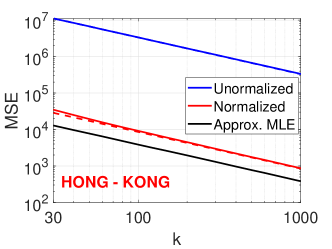
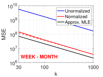
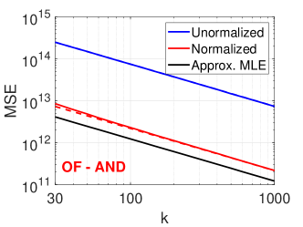
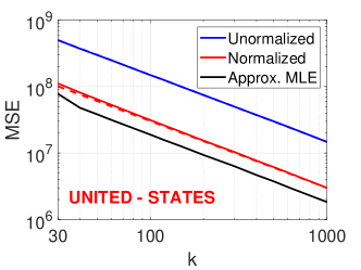
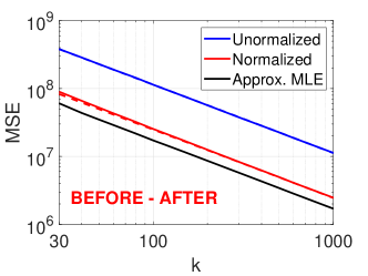
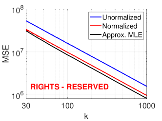
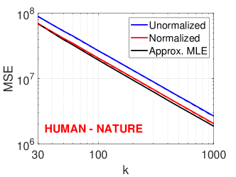
Figure 5: We estimate the inner products of the 9 pairs of words in Table 1, using the un-normalized estimator $\hat{a}$, the normalized estimator $\hat{a}_{n}$, as well as the approximate MLE estimator $\hat{a}_{m}$. We also plot, as dashed curves, the theoretical variances for $\hat{a}$ and $\hat{a}_{n}$. As expected, for $\hat{a}$, the empirical MSEs overlap with the theoretical variances. The normalized estimator $\hat{a}_{n}$ is considerably more accurate than $\hat{a}$, especially for word pairs with higher similarities. Also, for $\hat{a}_{n}$, the empirical MSEs do not differ much from the theoretical asymptotic variances. The “approximate MLE” $\hat{a}_{m}$ is still more accurate than the normalized estimator $\hat{a}_{n}$, although the differences are quite small.

Table 1 lists 9 word-pairs from the “Words” dataset (Li and Church, 2005). Basically, each word represents a vector of length $2^{16}$ and each entry of the vector records the number of documents that word appears in a collection of $2^{16}$ documents. The selected 9 pairs cover a variety of scenarios (high sparsity versus low similarity, high similarity versus low similarity, etc).

Next, we compare the two inner product estimators $\hat{a}$ and $\hat{a}_{n}$ for these 9 pairs of words. In order to provide a more complete picture, we also add another estimator based on the (approximate) maximum likelihood estimation (MLE). Because characterizing the exact joint distribution of $(x_{j},y_{j}),j=1,2,...,k$ would be too complicated, we resort to the MLE for the standard Gaussian random projections, as studied in Li et al. (2006a). Basically, they show that the estimator $\hat{a}_{m}$, which is the solution to the following cubic equation:

$$\hat{a}_{m}^{3}-\hat{a}_{m}^{2}\sum_{j=1}^{k}x_{j}y_{j}+\hat{a}_{m}\left(-\sum_{i=1}^{D}u_{i}^{2}\sum_{i=1}^{D}v_{i}^{2}+\sum_{i=1}^{D}u_{i}^{2}\sum_{j=1}^{k}y_{j}^{2}+\sum_{i=1}^{D}v_{i}^{2}\sum_{j=1}^{k}x_{j}^{2}\right)-\sum_{i=1}^{D}u_{i}^{2}\sum_{i=1}^{D}v_{i}^{2}\sum_{j=1}^{k}x_{j}y_{j}=0.$$

The MLE has the smallest estimation variance if the margins $\sum_{i=1}^{D}u_{i}^{2}$ and $\sum_{i=1}^{D}v_{i}^{2}$ are known. Obviously, the estimator $\hat{a}_{m}$ can no longer be written as an inner product (i.e., $\hat{a}_{m}$ is not a valid kernel for machine learning), unlike our $\hat{a}$ or $\hat{\rho}$ or $\hat{a}_{n}$. Nevertheless, we can still use the MLE to assess the accuracy of estimators to see how close they are to be optimal.

Although we do not know the exact MLE for OPORP, we still use the above cubic equation as the “surrogate” for the MLE equation of OPORP and plot the empirical MSEs together with the MSEs of $\hat{a}$ and $\hat{a}_{n}$ in Figure 5, for estimating the inner products of the 9 pairs of words in Table 1.

In each panel of Figure 5, we present 5 curves: the empirical MSEs for $\hat{a}$, $\hat{a}_{n}$, and $\hat{a}_{m}$, and the theoretical variances for $\hat{a}$ and $\hat{a}_{n}$. As expected, for $\hat{a}$ (the un-normalized estimator), the empirical MSEs overlap with the theoretical variances. The normalized estimator $\hat{a}_{n}$ is considerably more accurate than the un-normalized estimator $\hat{a}$, especially for word pairs with higher similarities. Also, for $\hat{a}_{n}$, the empirical MSEs do not differ much from the theoretical asymptotic variances, although they do not fully overlap. Interestingly, the “approximate MLE” $\hat{a}_{m}$ is still more accurate than the normalized estimator $\hat{a}_{n}$, although the differences are quite small.

Finally, Figure 6 compares VSRP (for its $s\in\{1,10,30,100,200\}$) with OPORP, for both the normalized and un-normalize estimator, using the “HONG-KONG” word pair. The plots confirm the theoretical result in Theorem 5. In this example, VSRP with $s=1$ has essentially the same MSEs as OPORP, as the theory predicts. Note that in this case $\frac{D-k}{D-1}$ is too small to be able to help OPORP to reduce the variance. As we increase $s$ for VSRP, the accuracy degrades quite substantially, again as predicted by the theory. We will observe the similar pattern in the experimental study in Section 4.

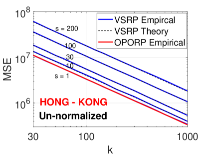
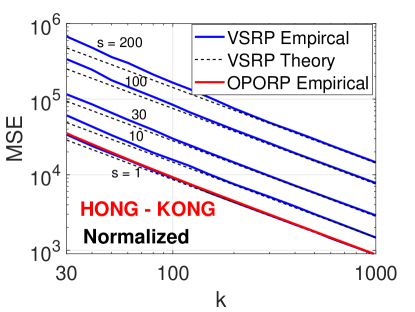
Figure 6: Comparing VSRP (with $s\in\{1,10,30,100,200\}$) with OPORP, in terms of their empirical MSEs, for both the un-normalized (left) and normalized (right) estimators, for the “HONG-KONG” word pair. As predicted by the theory, VSRP with $s=1$ essentially has the same accuracy as OPORP. Clearly, the normalized estimators are substantially more accurate than the un-normalized estimators. For the un-normalized VSRP estimator, the theoretical variance curves (dashed) overlap the solid MSE curves (solid). For the normalized VSRP estimator, the empirical MSEs slightly deviate from the theoretical variances (in Theorem 5) when $k$ is small.

4 Experiments

We conduct experiments on two standard datasets: the MNIST dataset with 60000 training samples and 10000 testing samples, and the ZIP dataset (zipcode) with 7291 training samples and 2007 testing samples. The data vectors are normalized to have the unit $l_{2}$ norm. The MNIST dataset has 784 features and the ZIP dataset has 256 features. These dimensions well correspond with typical EBR embedding vector sizes (i.e., $D=256\sim 1024$).

4.1 Retrieval

In this experiment, we do not use the class labels. We treat the data vectors in the test sets as query vectors. For each query vector, we compute/estimate the cosine similarities with all the data vectors in the training set. For each estimation method, we rank the retrieved data vectors according to the estimated cosine similarities. In other words, there will be two ranked lists, one using the true cosines and the other using estimated cosines. By walking down the lists, we can compute the precision and recall curves. This allows us to compare OPORP with VSRP and their various estimators. Again, since the original data are already normalized, the inner product estimators are also cosine estimators. This makes it convenient to present the comparisons.

Figure 7 presents the precision-recall curves for retrieving the top-50 candidates on MNIST. The curves for top-10 are pretty similar. As expected, the OPORP normalized estimator performs much better than the un-normalized inner product estimator of OPORP, for all $k\in\{32,64,128,256\}$. The comparisons with VSRP (parameterized by $s$) are very interesting. Recall that VSRP with $s=1$ has the same variance as the un-normalized estimator of OPORP except for the $\frac{D-k}{D-1}$ term. In Figure 7, it is clear that the un-normalized OPORP estimator performs better than VSRP, which is due to the $\frac{D-k}{D-1}$ term. This effect is especially obvious for $k=256$ and $k=128$. By increasing $s$ for VSRP, we can observe deteriorating performances. In particular, when $s=100$ (i.e., the projection matrix of VSRP is extremely sparse), the loss of accuracy might be unacceptable.

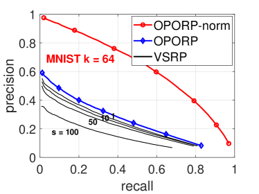
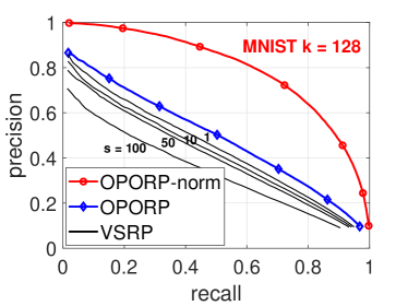
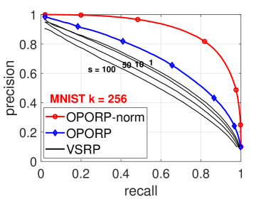
Figure 7: Precision-recall curves for MNIST (top-50) retrieval, using estimated cosines from the OPORP normalized estimator $\hat{\rho}$, the OPORP un-normalized estimator $\hat{a}$ (note that the original data are normalized), and the VSRP (parameterized by $s$) inner product estimator for $s\in\{1,10,50,100\}$.

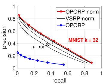
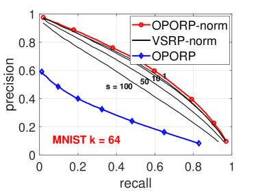
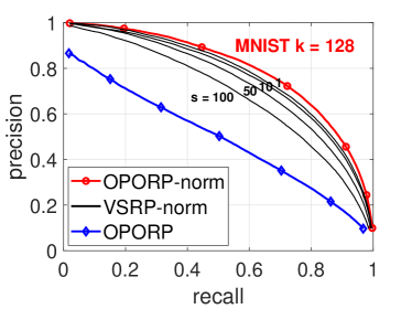
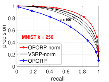
Figure 8: The content is pretty similar to that of Figure 7, but this time we normalize the estimator of VSRP (parameterized by $s\in\{1,10,50,100\}$).

Figure 8 is quite similar to Figure 7 except that Figure 8 presents the normalized inner product estimator of VSRP, again for $s\in\{1,10,50,100\}$. Indeed, as already shown by theory, the normalized estimator of VSRP improves the accuracy considerably. On the other hand, we still observe that, when $s=1$ for VSRP, its accuracy is slightly worse than OPORP (due to the $\frac{D-k}{D-1}$ factor); and when $s=100$, there is a severe deterioration of performance. Figure 8 once again confirms that the normalization trick is an excellent tool, which ought to be taken advantage of.

Figure 9 presents the (top-10) retrieval experiments on the ZIP dataset. The plots are analogous to the plots in Figure 7 and Figure 8, with essentially the same conclusion.

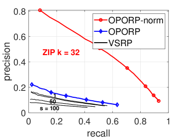
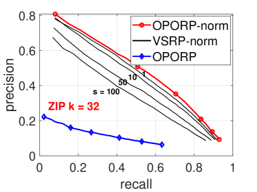
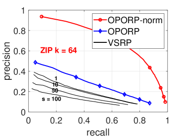
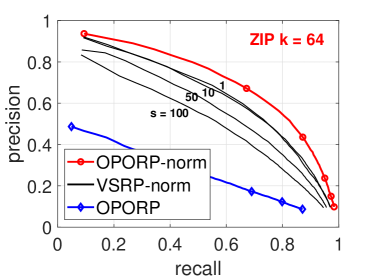
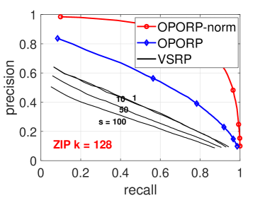
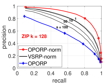
Figure 9: Precision-recall curves for ZIP (top-10) retrieval. The left panels are analogous to Figure 7 and the right panels are analogous to Figure 8 for MNIST retrieval.

4.2 KNN classification

Figure 10 presents the experiments on KNN (K nearest neighbors) classification, in particular 1-NN and 10-NN, for both MNIST and ZIP datasets. We need the class labels for this set of experiments. In each panel, the vertical axis represents the test classification accuracy (in $\%$). The original classification accuracy (the dashed horizontal curve) is pretty high, but we can approach the same accuracy with OPORP using the normalized estimator (with e.g., $k\geq 128$ for MNIST and $k\geq 64$ for ZIP). The performance of the un-normalized estimator of OPORP is considerably worse. Also, OPORP improves VSRP with $s=1$ owing to the $\frac{D-k}{D-1}$ factor. Again, using VSRP with large $s$ values leads to poor performance.

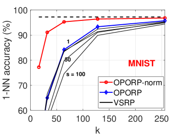
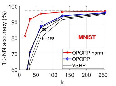
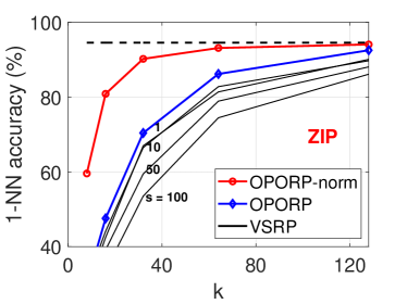
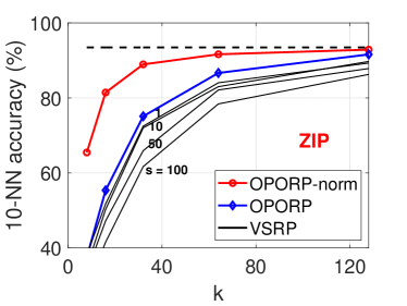
Figure 10: 1-NN and 10-NN classification results using cosines. The horizontal dashed lines represent the results using the true cosines. The general trends are pretty much the same as observed in the retrieval experiments in Figure 7. The vertical axis is the test classification accuracy. OPORP normalized estimator considerably improves OPORP un-normalized estimator. OPORP improves VSRP with $s=1$ (due to $\frac{D-k}{D-1}$). Again, using VSRP with large $s$ values leads to poor performance.

5 Differential Privacy: DP-OPORP and DP-SignOPORP

In a recent work (Li and Li, 2023), OPORP has been used as a basic building block for differential privacy (DP) (Dwork et al., 2006) for RP-type data compression. DP is a standard privacy definition defined as below, whose mathematical intuition is that the distribution of the algorithm output should stay close when the dataset is changed by a little.

Definition 5.1 (Differential Privacy (Dwork et al., 2006)).

For a randomized algorithm $\mathcal{M}:\mathcal{U}\mapsto Range(\mathcal{M})$, if for any two adjacent datasets $U$ and $U^{\prime}$, it holds that

$$Pr[\mathcal{M}(U)\in O]\leq e^{\epsilon}Pr[\mathcal{M}(U^{\prime})\in O]+\delta$$ (16)

for $\forall O\subset Range(\mathcal{M})$ and some $\epsilon,\delta\geq 0$, then algorithm $\mathcal{M}$ is called $(\epsilon,\delta)$-differentially private. If $\delta=0$, $\mathcal{M}$ is called $\epsilon$-differentially private.

The definition of “neighboring” is given as follows.

Definition 5.2 ($\beta$-adjacency).

Let $u\in[-1,1]^{p}$ be a data vector. A vector $u^{\prime}\in[-1,1]^{p}$ is said to be $\beta$-adjacent to $u$ if $u^{\prime}$ and $u$ differ in one dimension $i$, and $|u_{i}-u_{i}^{\prime}|\leq\beta$.

The privacy parameter $\beta$ is flexible depending on the application scenarios. Li and Li (2023) proposed two variants of OPORP under DP: the full-precision DP-OPORP and the 1-bit DP-SignOPORP for even higher data compression rate. We briefly introduce these algorithms as follows.

DP-OPORP.     The DP-OPORP method is summarized in Algorithm 1. We first produce the (non-DP) OPORP samples (in $\mathbb{R}^{k}$), and then add a random Gaussian noise vector to the OPORP. At Line 5, the Gaussian noise magnitude $\sigma$ is computed by solving the equation for $\sigma^{*}$:

$$\Phi\left(\frac{\triangle_{2}}{2\sigma}-\frac{\epsilon\sigma}{\triangle_{2}}\right)-e^{\epsilon}\Phi\left(-\frac{\triangle_{2}}{2\sigma}-\frac{\epsilon\sigma}{\triangle_{2}}\right)=\delta,$$ (17)

which is the “optimal Gaussian mechanism” (Balle and Wang, 2018), where $\triangle_{2}$ is the “$l_{2}$-sensitivity”. Algorithm 1 achieves $(\epsilon,\delta)$-DP, and is superior to the best DP variant for random projections (DP-RP) both theoretically (in terms of inner product estimation variance) and empirically (on similarity search and SVM classification). Figure 11 (from Li and Li (2023)) compares several DP algorithms based on random projections to confirm that DP-OPORP achieves the overall best performance.

1 Input: Data $u\in[-1,1]^{p}$, privacy parameters $\epsilon>0$, $\delta\in(0,1)$, number of projections $k$

2Output: Differentially private OPORP

3Generate the OPORP of $u$ as $x=OPORP(u)$

4Set sensitivity $\triangle_{2}=\beta$

5Generate iid random vector $G\in\mathbb{R}^{k}$ following $N(0,\sigma^{2})$ where $\sigma$ is computed by (17)

Return $\tilde{x}=x+G$

Algorithm 1 DP-OPORP (Li and Li, 2023)

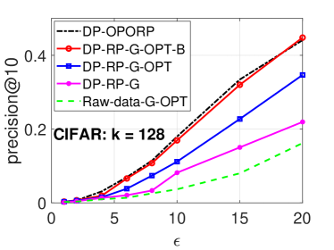
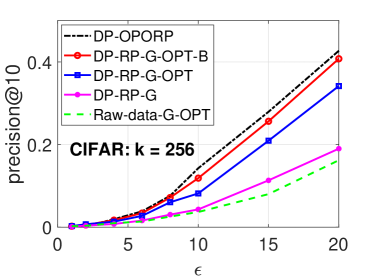
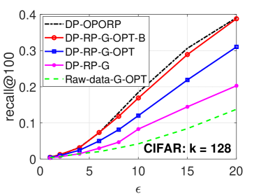
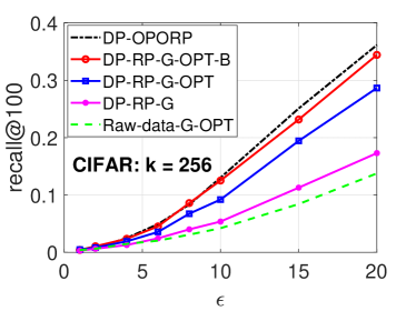
Figure 11: (Li and Li, 2023) Recall and precision on CIFAR, $\beta=1$, $\delta=10^{-6}$.

1 Input: Data $u\in[-1,1]^{p}$; $\epsilon>0$; Number of projections $k$

2

3Output: Differentially private sign OPORP

4

5Generate the OPORP of $u$ as $x=OPORP(u)$

6

DP-SignOPORP-RR:

7Compute $\tilde{s}_{j}=\begin{cases}sign(x_{j}),&\text{with prob.}\ \frac{e^{\epsilon}}{e^{\epsilon}+1}\\ -sign(x_{j}),&\text{with prob.}\ \frac{1}{e^{\epsilon}+1}\end{cases}$ for $j=1,...,k$

DP-SignOPORP-RR-smooth:

8Compute $L_{j}=\lceil\frac{|x_{j}|}{\beta}\rceil$ for $j=1,...,k$

9Compute $\tilde{s}_{j}=\begin{cases}sign(x_{j}),&\text{with prob.}\ \frac{e^{\epsilon_{j}^{\prime}}}{e^{\epsilon_{j}^{\prime}}+1}\\ -sign(x_{j}),&\text{with prob.}\ \frac{1}{e^{\epsilon_{j}^{\prime}}+1}\end{cases}$ for $j=1,...,k$, with $\epsilon_{j}^{\prime}=L_{j}\epsilon$

10For $\tilde{s}_{j}=0$, assign a random coin in $\{-1,1\}$

Return $\tilde{s}$ as the DP-SignRP of $u$

Algorithm 2 DP-SignOPORP-RR and DP-SignOPORP-RR-smooth (Li and Li, 2023)

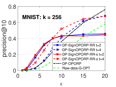
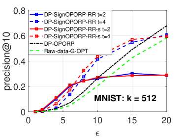
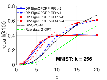
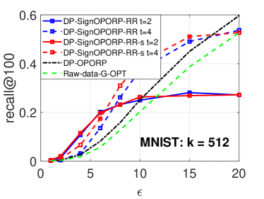
Figure 12: (Li and Li, 2023) Retrieval on MNIST with DP-SignOPORP-RR and DP-SignOPORP-RR-smooth (in the caption, “-s” stands for “-smooth”.

DP-SignOPORP.     The algorithm is summarized in Algorithm 2. We first generate the OPORP $x=OPORP(u)$, then takes the sign of $x$ to get a length-$k$ bit vector. Then, we have two options. The first “DP-SignOPORP-RR” strategy is to apply the standard/classic randomized response (RR) technique to flip each bit with probability $\frac{1}{e^{\epsilon}+1}$ and keep the true sign otherwise. The second (improved) solution, called “DP-SignOPORP-RR-smooth” is based on the concept proposed by Li and Li (2023) called “smooth flipping probability”, inspired by the work of Nissim et al. (2007). That is, the flipping probability for each bit is $\frac{1}{e^{\epsilon_{j}^{\prime}}+1}$ with $\epsilon_{j}^{\prime}=L_{j}\epsilon$ and $L_{j}=\lceil\frac{|x_{j}|}{\beta}\rceil$. The intuitive understanding is that, when the OPORP value is farther from $0$, the flipping probability of the sign of OPORP can be smaller. This is a consequence of the fact that the “aggregate-and-sign” operation of RP-type algorithms brings robustness against small changes in the data. It is proved that both approaches are $\epsilon$-DP. The DP-SignOPORP-RR-smooth has smaller flipping probability than DP-SignOPORP-RR and thus better utility. Li and Li (2023) also shown that applying multiple $t$ repetitions of DP-SignOPORP (each time with $k/t$ projections and privacy budget $\epsilon/t$) may help improve the performance of DP-SignOPORP. Figure 12 (also from Li and Li (2023)) confirms that DP-SignOPORP achieves good better performance than DP-OPORP especially when $\epsilon$ is not large.

Finally, We should mention that Li and Li (2023) also developed algorithms (e.g., iDP-SignRP) for “individual differential privacy” (iDP) (Soria-Comas et al., 2017) which are able to achieve remarkable utility performance even at very small $\epsilon$ (e.g., $\epsilon<0.5$).

6 Conclusion

Computing or estimating the inner products (or cosines) is the routine operation in numerous applications, not limited to machine learning. Reducing the storage/memory cost and speeding up the computations for computing/estimating the inner products or cosines can be crucial especially in many industrial applications such as embedding-based retrieval (EBR) for search and advertising.

The “one permutation + one random projection” (OPORP) is a variant of count-sketch and is closely related to “very sparse random projections” (VSRP). Compared to the standard random projections, OPORP is substantially more efficient (as it involves only one projection) and also more accurate. It differs from the standard count-sketch in that OPORP utilizes (i) the fixed-length binning scheme; (ii) the normalized estimator of cosine and inner product. We have conducted thorough variance analysis for OPORP (as well as VSRP) for both un-normalized and normalized estimators.

Among many applications (e.g., AI model compression), this work can be used as a key component in modern ANN (approximate near neighbor search) systems. For example, Zhao et al. (2020) developed the GPU graph-based ANN algorithm and used random projections to reduce memory cost when data do not in the memory. For large-scale graph-based ANN methods (Zhou et al., 2019; Malkov and Yashunin, 2020), the main cost is to compute similarities on the fly. We can effectively compress the vectors using OPORP to facilitate the distance computations at reduced storage.

As elaborated in the paper, OPORP and VSRP (very sparse random projections) (Li et al., 2006b) can be viewed as two extreme examples of sparse random projections. Our work on OPORP naturally recovers the estimator and theory of VSRP. In fact, as a by-product, we also develop the normalized estimator for VSRP and derive its variance. To compare VSRP with OPORP, the general conclusion is that both have the same variance (neglecting the beneficial $\frac{D-k}{D-1}$ factor for OPORP) if VSRP uses $s=1$ (i.e., a fully dense projection matrix); but VSRP can severely lose the accuracy if VSRP uses a large $s$ value in order to achieve the same level of sparsity as OPORP.

Appendix A Proof of Theorem 2

For two data vectors $u,v\in\mathbb{R}^{D}$, recall the notations of OPORP:

$$\hat{a}=\sum_{j=1}^{k}x_{j}y_{j},\hskip 14.45377ptx_{j}=\sum_{i=1}^{D}u_{i}r_{i}I_{ij},\hskip 14.45377pty_{j}=\sum_{i=1}^{D}v_{i}r_{i}I_{ij}.$$

Assume the random variable $r$ admits

$$E(r_{i})=0,\hskip 21.68121ptE(r_{i}^{2})=1,\hskip 21.68121ptE(r_{i}^{3})=0,\hskip 21.68121ptE(r_{i}^{4})=s.$$

Our goal is to show

$$E(\hat{a})=a,$$

$$Var(\hat{a}_{1})=\left(s-1\right)\sum_{i=1}^{D}u_{i}^{2}v_{i}^{2}+\frac{1}{k}\left[a^{2}+\sum_{i=1}^{D}u_{i}^{2}\sum_{i=1}^{D}v_{i}^{2}-2\sum_{i=1}^{D}u_{i}^{2}v_{i}^{2}\right]\frac{D-k}{D-1},$$

$$Var(\hat{a}_{2})=\left(s-1\right)\sum_{i=1}^{D}u_{i}^{2}v_{i}^{2}+\frac{1}{k}\left[a^{2}+\sum_{i=1}^{D}u_{i}^{2}\sum_{i=1}^{D}v_{i}^{2}-2\sum_{i=1}^{D}u_{i}^{2}v_{i}^{2}\right].$$

Firstly, for the mean, we have

$$E\left(\hat{a}\right)= E\left(\sum_{j=1}^{k}x_{j}y_{j}\right)=E\left(\sum_{j=1}^{k}\sum_{i=1}^{D}u_{i}r_{i}I_{ij}\sum_{i=1}^{D}v_{i}r_{i}I_{ij}\right)$$

$$= E\left(\sum_{j=1}^{k}\sum_{i=1}^{D}u_{i}v_{i}r_{i}^{2}I_{ij}^{2}+\sum_{i\neq i^{\prime}}u_{i}v_{i^{\prime}}r_{i}r_{i^{\prime}}I_{ij}I_{i^{\prime}j}\right)$$

$$= E\left(\sum_{j=1}^{k}\sum_{i=1}^{D}u_{i}v_{i}\frac{1}{k}\right)+0$$

$$= \sum_{i=1}^{D}u_{i}v_{i}=a,$$

which shows that $\hat{a}$ is an unbiased estimator of $a$.

We can compute the second moment of $\hat{a}$ as

$$E\left(\hat{a}^{2}\right)= E\left(\sum_{j=1}^{k}x_{j}y_{j}\right)^{2}=E\left(\sum_{j=1}^{k}\sum_{i=1}^{D}u_{i}r_{i}I_{ij}\sum_{i=1}^{D}v_{i}r_{i}I_{ij}\right)^{2}$$

$$= E\left(\sum_{j=1}^{k}\sum_{i=1}^{D}u_{i}v_{i}r_{i}^{2}I_{ij}^{2}+\sum_{i\neq i^{\prime}}u_{i}v_{i^{\prime}}r_{i}r_{i^{\prime}}I_{ij}I_{i^{\prime}j}\right)^{2}$$

$$= E\left(\sum_{j=1}^{k}\left(\sum_{i=1}^{D}u_{i}v_{i}r_{i}^{2}I_{ij}^{2}+\sum_{i\neq i^{\prime}}u_{i}v_{i^{\prime}}r_{i}r_{i^{\prime}}I_{ij}I_{i^{\prime}j}\right)^{2}\right)$$

$$+ E\left(\sum_{j\neq j^{\prime}}\left(\sum_{i=1}^{D}u_{i}v_{i}r_{i}^{2}I_{ij}^{2}+\sum_{i\neq i^{\prime}}u_{i}v_{i^{\prime}}r_{i}r_{i^{\prime}}I_{ij}I_{i^{\prime}j}\right)\left(\sum_{i=1}^{D}u_{i}v_{i}r_{i}^{2}I_{ij^{\prime}}^{2}+\sum_{i\neq i^{\prime}}u_{i}v_{i^{\prime}}r_{i}r_{i^{\prime}}I_{ij^{\prime}}I_{i^{\prime}j^{\prime}}\right)\right)$$

$$= \sum_{j=1}^{k}E\left(\sum_{i=1}^{D}u_{i}v_{i}r_{i}^{2}I_{ij}^{2}+\sum_{i\neq i^{\prime}}u_{i}v_{i^{\prime}}r_{i}r_{i^{\prime}}I_{ij}I_{i^{\prime}j}\right)^{2}$$

$$+ \sum_{j\neq j^{\prime}}E\left(\sum_{i=1}^{D}u_{i}v_{i}r_{i}^{2}I_{ij}^{2}+\sum_{i\neq i^{\prime}}u_{i}v_{i^{\prime}}r_{i}r_{i^{\prime}}I_{ij}I_{i^{\prime}j}\right)\left(\sum_{i=1}^{D}u_{i}v_{i}r_{i}^{2}I_{ij^{\prime}}^{2}+\sum_{i\neq i^{\prime}}u_{i}v_{i^{\prime}}r_{i}r_{i^{\prime}}I_{ij^{\prime}}I_{i^{\prime}j^{\prime}}\right).$$ (18)

We now compute the two terms separately. For the first term, we have

$$E\left(\sum_{i=1}^{D}u_{i}v_{i}r_{i}^{2}I_{ij}^{2}+\sum_{i\neq i^{\prime}}u_{i}v_{i^{\prime}}r_{i}r_{i^{\prime}}I_{ij}I_{i^{\prime}j}\right)^{2}$$

$$= E\left(\sum_{i=1}^{D}u_{i}v_{i}r_{i}^{2}I_{ij}^{2}\right)^{2}+E\left(\sum_{i\neq i^{\prime}}u_{i}v_{i^{\prime}}r_{i}r_{i^{\prime}}I_{ij}I_{i^{\prime}j}\right)^{2}+2E\left(\sum_{i=1}^{D}u_{i}v_{i}r_{i}^{2}I_{ij}^{2}\right)\left(\sum_{i\neq i^{\prime}}u_{i}v_{i^{\prime}}r_{i}r_{i^{\prime}}I_{ij}I_{i^{\prime}j}\right)$$

$$= s\frac{1}{k}\sum_{i=1}^{D}u_{i}^{2}v_{i}^{2}+\sum_{i\neq i^{\prime}}u_{i}v_{i}u_{i^{\prime}}v_{i^{\prime}}E\left(I_{ij}I_{i^{\prime}j}\right)+\sum_{i\neq i^{\prime}}u_{i}^{2}v_{i^{\prime}}^{2}E(I_{ij}I_{i^{\prime}j})+\sum_{i\neq i^{\prime}}u_{i}v_{i}u_{i^{\prime}}v_{i^{\prime}}E\left(I_{ij}I_{i^{\prime}j}\right)$$

$$= s\frac{1}{k}\sum_{i=1}^{D}u_{i}^{2}v_{i}^{2}+\sum_{i\neq i^{\prime}}\left(u_{i}^{2}v_{i^{\prime}}^{2}+2u_{i}v_{i}u_{i^{\prime}}v_{i^{\prime}}\right)E\left(I_{ij}I_{i^{\prime}j}\right)$$

To see the above calculations, we can calculate the three terms respectively.

$$E\left(\sum_{i=1}^{D}u_{i}v_{i}r_{i}^{2}I_{ij}^{2}\right)^{2}= E\left(\sum_{i=1}^{D}u_{i}^{2}v_{i}^{2}r_{i}^{4}I_{ij}^{4}\right)+E\left(\sum_{i\neq i^{\prime}}u_{i}v_{i}r_{i}^{2}I_{ij}^{2}u_{i^{\prime}}v_{i^{\prime}}r_{i^{\prime}}^{2}I_{i^{\prime}j}^{2}\right)$$

$$= s\frac{1}{k}\sum_{i=1}^{D}u_{i}^{2}v_{i}^{2}+\sum_{i\neq i^{\prime}}u_{i}v_{i}u_{i^{\prime}}v_{i^{\prime}}E\left(I_{ij}I_{i^{\prime}j}\right),$$

$$E\left(\sum_{i\neq i^{\prime}}u_{i}v_{i^{\prime}}r_{i}r_{i^{\prime}}I_{ij}I_{i^{\prime}j}\right)^{2}$$

$$= E\left(\sum_{i<i^{\prime}}u_{i}v_{i^{\prime}}r_{i}r_{i^{\prime}}I_{ij}I_{i^{\prime}j}+\sum_{i>i^{\prime}}u_{i}v_{i^{\prime}}r_{i}r_{i^{\prime}}I_{ij}I_{i^{\prime}j}\right)^{2}$$

$$= E\left(\sum_{i\neq i^{\prime}}u_{i}^{2}v_{i^{\prime}}^{2}r_{i}^{2}r_{i^{\prime}}^{2}I_{ij}^{2}I_{i^{\prime}j}^{2}\right)+2E\left(\sum_{i<i^{\prime}}u_{i}v_{i^{\prime}}r_{i}r_{i^{\prime}}I_{ij}I_{i^{\prime}j}\right)\left(\sum_{i<i^{\prime}}u_{i^{\prime}}v_{i}r_{i}r_{i^{\prime}}I_{ij}I_{i^{\prime}j}\right)$$

$$= \sum_{i\neq i^{\prime}}u_{i}^{2}v_{i^{\prime}}^{2}E(I_{ij}I_{i^{\prime}j})+2\sum_{i<i^{\prime}}u_{i}u_{i^{\prime}}v_{i}v_{i^{\prime}}E\left(I_{ij}I_{i^{\prime}j}\right)$$

$$= \sum_{i\neq i^{\prime}}u_{i}^{2}v_{i^{\prime}}^{2}E(I_{ij}I_{i^{\prime}j})+\sum_{i\neq i^{\prime}}u_{i}u_{i^{\prime}}v_{i}v_{i^{\prime}}E\left(I_{ij}I_{i^{\prime}j}\right),$$

and

$$E\left(\sum_{i=1}^{D}u_{i}v_{i}r_{i}^{2}I_{ij}^{2}\right)\left(\sum_{i\neq i^{\prime}}u_{i}v_{i^{\prime}}r_{i}r_{i^{\prime}}I_{ij}I_{i^{\prime}j}\right)=0.$$

In the calculations, we can simplify the algebra by noting that $r_{i}$’s are i.i.d. and $E(r_{i})=E(r_{i}^{3})=0$. Next, we compute

$$E\left(\sum_{i=1}^{D}u_{i}v_{i}r_{i}^{2}I_{ij}^{2}+\sum_{i\neq i^{\prime}}u_{i}v_{i^{\prime}}r_{i}r_{i^{\prime}}I_{ij}I_{i^{\prime}j}\right)\left(\sum_{i=1}^{D}u_{i}v_{i}r_{i}^{2}I_{ij^{\prime}}^{2}+\sum_{i\neq i^{\prime}}u_{i}v_{i^{\prime}}r_{i}r_{i^{\prime}}I_{ij^{\prime}}I_{i^{\prime}j^{\prime}}\right)$$

$$= E\left(\sum_{i=1}^{D}u_{i}v_{i}r_{i}^{2}I_{ij}^{2}\right)\left(\sum_{i=1}^{D}u_{i}v_{i}r_{i}^{2}I_{ij^{\prime}}^{2}\right)+E\left(\sum_{i\neq i^{\prime}}u_{i}v_{i^{\prime}}r_{i}r_{i^{\prime}}I_{ij}I_{i^{\prime}j}\right)\left(\sum_{i\neq i^{\prime}}u_{i}v_{i^{\prime}}r_{i}r_{i^{\prime}}I_{ij^{\prime}}I_{i^{\prime}j^{\prime}}\right)$$

$$= s\sum_{i=1}^{D}u_{i}^{2}v_{i}^{2}E\left(I_{ij}I_{ij^{\prime}}\right)+\sum_{i\neq i^{\prime}}u_{i}v_{i}u_{i^{\prime}}v_{i^{\prime}}E\left(I_{ij}I_{i^{\prime}j^{\prime}}\right)+\sum_{i\neq i^{\prime}}u_{i}^{2}v_{i^{\prime}}^{2}E\left(I_{ij}I_{i^{\prime}j}I_{ij^{\prime}}I_{i^{\prime}j^{\prime}}\right)+\sum_{i\neq i^{\prime}}u_{i}u_{i^{\prime}}v_{i}v_{i^{\prime}}E\left(I_{ij}I_{i^{\prime}j}I_{ij^{\prime}}I_{i^{\prime}j^{\prime}}\right)$$

$$= \sum_{i\neq i^{\prime}}u_{i}v_{i}u_{i^{\prime}}v_{i^{\prime}}E\left(I_{ij}I_{i^{\prime}j^{\prime}}\right),$$

where we have used the fact that $I_{ij}I_{ij^{\prime}}=0$ always. Now turning back to (18), we obtain

$$E(\hat{a}^{2})= \sum_{j=1}^{k}\left[s\frac{1}{k}\sum_{i=1}^{D}u_{i}^{2}v_{i}^{2}+\sum_{i\neq i^{\prime}}\left(u_{i}^{2}v_{i^{\prime}}^{2}+2u_{i}v_{i}u_{i^{\prime}}v_{i^{\prime}}\right)E\left(I_{ij}I_{i^{\prime}j}\right)\right]+\sum_{j\neq j^{\prime}}\left[\sum_{i\neq i^{\prime}}u_{i}v_{i}u_{i^{\prime}}v_{i^{\prime}}E\left(I_{ij}I_{i^{\prime}j^{\prime}}\right)\right]$$

$$= s\sum_{i=1}^{D}u_{i}^{2}v_{i}^{2}+kE\left(I_{ij}I_{i^{\prime}j}\right)\sum_{i\neq i^{\prime}}\left(u_{i}^{2}v_{i^{\prime}}^{2}+2u_{i}v_{i}u_{i^{\prime}}v_{i^{\prime}}\right)+k(k-1)E\left(I_{ij}I_{i^{\prime}j^{\prime}}\right)\sum_{i\neq i^{\prime}}u_{i}v_{i}u_{i^{\prime}}v_{i^{\prime}}.$$

Therefore, the variance can be expressed as

$$Var(\hat{a})=E(\hat{a}^{2})-a^{2}$$

$$= s\sum_{i=1}^{D}u_{i}^{2}v_{i}^{2}+kE\left(I_{ij}I_{i^{\prime}j}\right)\sum_{i\neq i^{\prime}}\left(u_{i}^{2}v_{i^{\prime}}^{2}+2u_{i}v_{i}u_{i^{\prime}}v_{i^{\prime}}\right)+k(k-1)E\left(I_{ij}I_{i^{\prime}j^{\prime}}\right)\sum_{i\neq i^{\prime}}u_{i}v_{i}u_{i^{\prime}}v_{i^{\prime}}-\left(\sum_{i=1}^{D}u_{i}v_{i}\right)^{2}$$

$$= \left(s-1\right)\sum_{i=1}^{D}u_{i}^{2}v_{i}^{2}+kE\left(I_{ij}I_{i^{\prime}j}\right)\sum_{i\neq i^{\prime}}u_{i}^{2}v_{i^{\prime}}^{2}+\left[2kE\left(I_{ij}I_{i^{\prime}j}\right)+k(k-1)E\left(I_{ij}I_{i^{\prime}j^{\prime}}\right)-1\right]\sum_{i\neq i^{\prime}}u_{i}v_{i}u_{i^{\prime}}v_{i^{\prime}}$$

$$= \left(s-1\right)\sum_{i=1}^{D}u_{i}^{2}v_{i}^{2}+kE\left(I_{ij}I_{i^{\prime}j}\right)\sum_{i\neq i^{\prime}}u_{i}^{2}v_{i^{\prime}}^{2}+kE\left(I_{ij}I_{i^{\prime}j}\right)\sum_{i\neq i^{\prime}}u_{i}v_{i}u_{i^{\prime}}v_{i^{\prime}}$$

$$= \left(s-1\right)\sum_{i=1}^{D}u_{i}^{2}v_{i}^{2}+kE\left(I_{ij}I_{i^{\prime}j}\right)\left[\sum_{i=1}^{D}u_{i}^{2}\sum_{i=1}^{D}v_{i}^{2}-\sum_{i=1}^{D}u_{i}^{2}v_{i}^{2}+\left(\sum_{i=1}^{D}u_{i}v_{i}\right)^{2}-\sum_{i=1}^{D}u_{i}^{2}v_{i}^{2}\right]$$

$$= \left(s-1\right)\sum_{i=1}^{D}u_{i}^{2}v_{i}^{2}+kE\left(I_{ij}I_{i^{\prime}j}\right)\left[a^{2}+\sum_{i=1}^{D}u_{i}^{2}\sum_{i=1}^{D}v_{i}^{2}-2\sum_{i=1}^{D}u_{i}^{2}v_{i}^{2}\right].$$

The remaining part is to compute $E(I_{ij}I_{i^{\prime}j})$ for the two binning schemes respectively, which is finished by leveraging Lemma 1. $\hfill\qed$

Appendix B Proof of Theorem 4

Recall the notation in OPORP:

$$x_{j}=\sum_{i=1}^{D}u_{i}r_{i}I_{ij},\hskip 21.68121pty_{j}=\sum_{i=1}^{D}v_{i}r_{i}I_{ij},\hskip 14.45377ptj=1,2,...,k.$$

To analyze the normalized cosine estimator:

$$\hat{\rho}=\frac{\sum_{j=1}^{k}x_{j}y_{j}}{\sqrt{\sum_{j=1}^{k}x_{j}^{2}}{\sqrt{\sum_{j=1}^{k}y_{j}^{2}}}},$$

it suffices to assume the original data are normalized to unit $l_{2}$ norms, i.e., $\sum_{i=1}^{D}u_{i}^{2}=\sum_{i=1}^{D}v_{i}^{2}=1$. When the data are normalized, the inner product and the cosine are the same, i.e., $a=\rho$. Thus,

$$E\left(\sum_{j=1}^{k}x_{j}y_{j}\right)=\rho,\hskip 14.45377ptE\left(\sum_{j=1}^{k}x_{j}^{2}\right)=E\left(\sum_{j=1}^{k}y_{j}^{2}\right)=1,\hskip 14.45377pt$$

Via the Taylor expansion, we have

$$\hat{\rho}-\rho= \frac{\sum_{j=1}^{k}x_{j}y_{j}-\rho}{\sqrt{\sum_{j=1}^{k}x_{j}^{2}}{\sqrt{\sum_{j=1}^{k}y_{j}^{2}}}}+\rho\frac{1-\sqrt{\sum_{j=1}^{k}x_{j}^{2}}{\sqrt{\sum_{j=1}^{k}y_{j}^{2}}}}{\sqrt{\sum_{j=1}^{k}x_{j}^{2}}{\sqrt{\sum_{j=1}^{k}y_{j}^{2}}}}$$

$$= \sum_{j=1}^{k}x_{j}y_{j}-\rho+\rho\left(1-\sum_{j=1}^{k}x_{j}^{2}\right)/2+\rho\left(1-\sum_{j=1}^{k}y_{j}^{2}\right)/2+O_{P}\left(1/k\right)$$

$$= \sum_{j=1}^{k}x_{j}y_{j}-\rho/2\sum_{j=1}^{k}x_{j}^{2}-\rho/2\sum_{j=1}^{k}y_{j}^{2}+O_{P}\left(1/k\right),$$

where we use the approximation: for $a\approx 1$ and $b\approx 1$, $1-ab=(1-a)+(1-b)-(1-a)(1-b)$. It thus suffices to analyze the following term:

$$\left(\sum_{j=1}^{k}x_{j}y_{j}-\rho/2\sum_{j=1}^{k}x_{j}^{2}-\rho/2\sum_{j=1}^{k}y_{j}^{2}\right)^{2}$$

$$= \left(\sum_{j=1}^{k}x_{j}y_{j}\right)^{2}+\rho^{2}/4\left(\sum_{j=1}^{k}x_{j}^{2}+\sum_{j=1}^{k}y_{j}^{2}\right)^{2}-\rho\left(\sum_{j=1}^{k}x_{j}y_{j}\right)\left(\sum_{j=1}^{k}x_{j}^{2}+\sum_{j=1}^{k}y_{j}^{2}\right).$$ (19)

By Theorem 2, we know that

$$E\left(\sum_{j=1}^{k}x_{j}y_{j}\right)^{2}=\left(s-1\right)\sum_{i=1}^{D}u_{i}^{2}v_{i}^{2}+kE\left(I_{ij}I_{i^{\prime}j}\right)\left[1+\rho^{2}-2\sum_{i=1}^{D}u_{i}^{2}v_{i}^{2}\right]+\rho^{2},$$ (20)

and we can write

$$E\left(\sum_{j=1}^{k}x_{j}^{2}\sum_{j=1}^{k}y_{j}^{2}\right)=E\left(\sum_{j=1}^{k}x_{j}^{2}y_{j}^{2}+\sum_{j\neq j^{\prime}}^{k}x_{j}^{2}y_{j^{\prime}}^{2}\right).$$

We now calculate each term. First, we have for $j=1,...,k$,

$$E\left(x_{j}^{2}y_{j}^{2}\right)=s\frac{1}{k}\sum_{i=1}^{D}u_{i}^{2}v_{i}^{2}+E\left(I_{ij}I_{i^{\prime}j}\right)\sum_{i\neq i^{\prime}}\left(u_{i}^{2}v_{i^{\prime}}^{2}+2u_{i}v_{i}u_{i^{\prime}}v_{i^{\prime}}\right).$$

Also, for $j\neq j^{\prime}$,

$$E(x_{j}^{2}y_{j^{\prime}}^{2})=E\left(\sum_{i=1}^{D}u_{i}r_{i}I_{ij}\right)^{2}\left(\sum_{i=1}^{D}v_{i}r_{i}I_{ij^{\prime}}\right)^{2}$$

$$= E\left(\sum_{i=1}^{D}u_{i}^{2}r_{i}^{2}I_{ij}+\sum_{i\neq i^{\prime}}u_{i}u_{i^{\prime}}r_{i}r_{i^{\prime}}r_{i^{\prime}j}I_{ij}I_{i^{\prime}j}\right)\left(\sum_{i=1}^{D}v_{i}^{2}r_{i}^{2}I_{ij^{\prime}}+\sum_{i\neq i^{\prime}}v_{i}v_{i^{\prime}}r_{i}r_{i^{\prime}}r_{i^{\prime}j}I_{ij^{\prime}}I_{i^{\prime}j^{\prime}}\right)$$

$$= E\left(\sum_{i=1}^{D}u_{i}^{2}r_{i}^{2}I_{ij}\right)\left(\sum_{i=1}^{D}v_{i}^{2}r_{i}^{2}I_{ij^{\prime}}\right)+E\left(\sum_{i\neq i^{\prime}}u_{i}u_{i^{\prime}}r_{i}r_{i^{\prime}}r_{i^{\prime}j}I_{ij}I_{i^{\prime}j}\right)\left(\sum_{i\neq i^{\prime}}v_{i}v_{i^{\prime}}r_{i}r_{i^{\prime}}r_{i^{\prime}j}I_{ij^{\prime}}I_{i^{\prime}j^{\prime}}\right)$$

$$= E\left(I_{ij}I_{i^{\prime}j^{\prime}}\right)\sum_{i\neq i^{\prime}}u_{i}^{2}v_{i^{\prime}}^{2}.$$

Therefore, we obtain that

$$E\left(\sum_{j=1}^{k}x_{j}^{2}\sum_{j=1}^{k}y_{j}^{2}\right)=E\left(\sum_{j=1}^{k}x_{j}^{2}y_{j}^{2}+\sum_{j\neq j}^{k}x_{j}^{2}y_{j^{\prime}}^{2}\right)$$

$$= s\sum_{i=1}^{D}u_{i}^{2}v_{i}^{2}+kE\left(I_{ij}I_{i^{\prime}j}\right)\sum_{i\neq i^{\prime}}\left(u_{i}^{2}v_{i^{\prime}}^{2}+2u_{i}v_{i}u_{i^{\prime}}v_{i^{\prime}}\right)+k(k-1)E\left(I_{ij}I_{i^{\prime}j^{\prime}}\right)\sum_{i\neq i^{\prime}}u_{i}^{2}v_{i^{\prime}}^{2},$$

which leads to

$$E\left(\sum_{j=1}^{k}x_{j}^{2}+\sum_{j=1}^{k}y_{j}^{2}\right)^{2}=\left(s-1\right)\sum_{i=1}^{D}(u_{i}^{4}+v_{i}^{4})+2kE\left(I_{ij}I_{i^{\prime}j}\right)\left[2-\sum_{i=1}^{D}(u_{i}^{4}+v_{i}^{4})\right]+2$$

$$\hskip 14.45377pt+2s\sum_{i=1}^{D}u_{i}^{2}v_{i}^{2}+2kE\left(I_{ij}I_{i^{\prime}j}\right)\sum_{i\neq i^{\prime}}\left(u_{i}^{2}v_{i^{\prime}}^{2}+2u_{i}v_{i}u_{i^{\prime}}v_{i^{\prime}}\right)+2k(k-1)E\left(I_{ij}I_{i^{\prime}j^{\prime}}\right)\sum_{i\neq i^{\prime}}u_{i}^{2}v_{i^{\prime}}^{2}.$$ (21)

We now analyze the third term in (19). It holds that

$$E\left(\sum_{j=1}^{k}x_{j}y_{j}\right)\left(\sum_{j=1}^{k}x_{j}^{2}+\sum_{j=1}^{k}y_{j}^{2}\right)=E\left(\sum_{j=1}^{k}x_{j}^{3}y_{j}+\sum_{j\neq j}x_{j}y_{j}x_{j^{\prime}}^{2}\right)+E\left(\sum_{j=1}^{k}x_{j}y_{j}^{3}+\sum_{j\neq j}x_{j}y_{j}y_{j^{\prime}}^{2}\right).$$

We have

$$E(x_{j}y_{j}^{3})=E\left(\sum_{i=1}^{D}u_{i}r_{i}I_{ij}\right)\left(\sum_{i=1}^{D}v_{i}r_{i}I_{ij}\right)^{3}$$

$$= E\left(\sum_{i=1}^{D}u_{i}v_{i}r_{i}^{2}I_{ij}+\sum_{i\neq i^{\prime}}u_{i}v_{i^{\prime}}r_{i}r_{i^{\prime}}I_{ij}I_{i^{\prime}j}\right)\left(\sum_{i=1}^{D}v_{i}^{2}r_{i}^{2}I_{ij}+\sum_{i\neq i^{\prime}}v_{i}v_{i^{\prime}}r_{i}r_{i^{\prime}}I_{ij}I_{i^{\prime}j}\right)$$

$$= E\left(\sum_{i=1}^{D}u_{i}v_{i}r_{i}^{2}I_{ij}\right)\left(\sum_{i=1}^{D}v_{i}^{2}r_{i}^{2}I_{ij}\right)+E\left(\sum_{i\neq i^{\prime}}u_{i}v_{i^{\prime}}r_{i}r_{i^{\prime}}I_{ij}I_{i^{\prime}j}\right)\left(\sum_{i\neq i^{\prime}}v_{i}v_{i^{\prime}}r_{i}r_{i^{\prime}}I_{ij}I_{i^{\prime}j}\right)$$

$$= E\left(\sum_{i=1}^{D}u_{i}v_{i}^{3}r_{i}^{4}I_{ij}+\sum_{i\neq i^{\prime}}u_{i}v_{i}v_{i^{\prime}}^{2}r_{i}^{2}r_{i^{\prime}}^{2}I_{ij}I_{i^{\prime}j}\right)+E\left(\sum_{i\neq i^{\prime}}u_{i}v_{i^{\prime}}r_{i}r_{i^{\prime}}I_{ij}I_{i^{\prime}j}\right)\left(\sum_{i\neq i^{\prime}}v_{i}v_{i^{\prime}}r_{i}r_{i^{\prime}}I_{ij}I_{i^{\prime}j}\right)$$

$$= \frac{s}{k}\sum_{i=1}^{D}u_{i}v_{i}^{3}+\sum_{i\neq i^{\prime}}u_{i}v_{i}v_{i^{\prime}}^{2}E(I_{ij}I_{i^{\prime}j})+2\sum_{i\neq i^{\prime}}u_{i}v_{i}v_{i^{\prime}}^{2}E(I_{ij}I_{i^{\prime}j})$$

$$= \frac{s}{k}\sum_{i=1}^{D}u_{i}v_{i}^{3}+3E(I_{ij}I_{i^{\prime}j})\sum_{i\neq i^{\prime}}u_{i}v_{i}v_{i^{\prime}}^{2},$$

where we use the following computation:

$$E\left(\sum_{i<i^{\prime}}u_{i}v_{i^{\prime}}r_{i}r_{i^{\prime}}I_{ij}I_{i^{\prime}j}+\sum_{i>i^{\prime}}u_{i}v_{i^{\prime}}r_{i}r_{i^{\prime}}I_{ij}I_{i^{\prime}j}\right)\left(\sum_{i<i^{\prime}}v_{i}v_{i^{\prime}}r_{i}r_{i^{\prime}}I_{ij}I_{i^{\prime}j}+\sum_{i>i^{\prime}}v_{i}v_{i^{\prime}}r_{i}r_{i^{\prime}}I_{ij}I_{i^{\prime}j}\right)$$

$$= \sum_{i\neq i^{\prime}}u_{i}v_{i}v_{i^{\prime}}^{2}E(I_{ij}I_{i^{\prime}j})+E\left(\sum_{i<i^{\prime}}u_{i}v_{i^{\prime}}r_{i}r_{i^{\prime}}I_{ij}I_{i^{\prime}j}\right)\left(\sum_{i>i^{\prime}}v_{i}v_{i^{\prime}}r_{i}r_{i^{\prime}}I_{ij}I_{i^{\prime}j}\right)$$

$$\hskip 108.405pt+E\left(\sum_{i>i^{\prime}}u_{i}v_{i^{\prime}}r_{i}r_{i^{\prime}}I_{ij}I_{i^{\prime}j}\right)\left(\sum_{i<i^{\prime}}v_{i}v_{i^{\prime}}r_{i}r_{i^{\prime}}I_{ij}I_{i^{\prime}j}\right)$$

$$= \sum_{i\neq i^{\prime}}u_{i}v_{i}v_{i^{\prime}}^{2}E(I_{ij}I_{i^{\prime}j})+E\left(\sum_{i<i^{\prime}}u_{i}v_{i^{\prime}}r_{i}r_{i^{\prime}}I_{ij}I_{i^{\prime}j}\right)\left(\sum_{i<i^{\prime}}v_{i}v_{i^{\prime}}r_{i}r_{i^{\prime}}I_{ij}I_{i^{\prime}j}\right)$$

$$\hskip 108.405pt+E\left(\sum_{i<i^{\prime}}u_{i^{\prime}}v_{i}r_{i}r_{i^{\prime}}I_{ij}I_{i^{\prime}j}\right)\left(\sum_{i<i^{\prime}}v_{i}v_{i^{\prime}}r_{i}r_{i^{\prime}}I_{ij}I_{i^{\prime}j}\right)$$

$$= \sum_{i\neq i^{\prime}}u_{i}v_{i}v_{i^{\prime}}^{2}E(I_{ij}I_{i^{\prime}j})+\sum_{i<i^{\prime}}u_{i}v_{i}v_{i^{\prime}}^{2}E(I_{ij}I_{i^{\prime}j})+\sum_{i<i^{\prime}}u_{i^{\prime}}v_{i}^{2}v_{i^{\prime}}E(I_{ij}I_{i^{\prime}j})$$

$$= 2\sum_{i\neq i^{\prime}}u_{i}v_{i}v_{i^{\prime}}^{2}E(I_{ij}I_{i^{\prime}j}).$$

Furthermore, we have

$$E\left(x_{j}y_{j}x_{j^{\prime}}^{2}\right)=E\left(\sum_{i=1}^{D}u_{i}r_{i}I_{ij}\right)\left(\sum_{i=1}^{D}v_{i}r_{i}I_{ij}\right)\left(\sum_{i=1}^{D}u_{i}r_{i}I_{ij^{\prime}}\right)^{2}$$

$$= E\left(\sum_{i=1}^{D}u_{i}v_{i}r_{i}^{2}I_{ij}+\sum_{i\neq i^{\prime}}u_{i}v_{i^{\prime}}r_{i}r_{i^{\prime}}I_{ij}I_{i^{\prime}j}\right)\left(\sum_{i=1}^{D}u_{i}^{2}r_{i}^{2}I_{ij^{\prime}}+\sum_{i\neq i}u_{i}u_{i^{\prime}}r_{i}r_{i^{\prime}}I_{ij^{\prime}}I_{i^{\prime}j^{\prime}}\right)$$

$$= E(I_{ij}I_{i^{\prime}j^{\prime}})\sum_{i\neq i}u_{i}u_{i^{\prime}}^{2}v_{i}.$$

Thus, by symmetry we have

$$E\left(\sum_{j=1}^{k}x_{j}y_{j}\right)\left(\sum_{j=1}^{k}x_{j}^{2}+\sum_{j=1}^{k}y_{j}^{2}\right)=E\left(\sum_{j=1}^{k}x_{j}^{3}y_{j}+\sum_{j\neq j}x_{j}y_{j}x_{j^{\prime}}^{2}\right)+E\left(\sum_{j=1}^{k}x_{j}y_{j}^{3}+\sum_{j\neq j}x_{j}y_{j}y_{j^{\prime}}^{2}\right)$$

$$= s\sum_{i=1}^{D}\left(u_{i}v_{i}^{3}+u_{i}^{3}v_{i}\right)+3kE(I_{ij}I_{i^{\prime}j})\sum_{i\neq i^{\prime}}\left(u_{i}v_{i}v_{i^{\prime}}^{2}+u_{i}v_{i}u_{i^{\prime}}^{2}\right)+k(k-1)E(I_{ij}I_{i^{\prime}j^{\prime}})\sum_{i\neq i}\left(u_{i}u_{i^{\prime}}^{2}v_{i}+u_{i}v_{i^{\prime}}^{2}v_{i}\right).$$ (22)

Now we combine (20), (21) and (22) with (19) to obtain

$$\left(\sum_{j=1}^{k}x_{j}y_{j}-\rho/2\sum_{j=1}^{k}x_{j}^{2}-\rho/2\sum_{j=1}^{k}y_{j}^{2}\right)^{2}$$

$$= (s-1)\sum_{i=1}^{D}\left((1+\rho^{2}/2)u_{i}^{2}v_{i}^{2}+\rho^{2}u_{i}^{4}/4+\rho^{2}v_{i}^{4}/4-\rho u_{i}v_{i}^{3}-\rho u_{i}^{3}v_{i}\right)$$

$$+kE\left(I_{ij}I_{i^{\prime}j}\right)\left[1+\rho^{2}-2\sum_{i=1}^{D}u_{i}^{2}v_{i}^{2}\right]+\rho^{2}kE\left(I_{ij}I_{i^{\prime}j}\right)\left[1-\sum_{i=1}^{D}(u_{i}^{4}+v_{i}^{4})/2\right]$$

$$+\rho^{2}\left[3+\sum_{i=1}^{D}u_{i}^{2}v_{i}^{2}+kE\left(I_{ij}I_{i^{\prime}j}\right)\sum_{i\neq i^{\prime}}\left(u_{i}^{2}v_{i^{\prime}}^{2}+2u_{i}v_{i}u_{i^{\prime}}v_{i^{\prime}}\right)+k(k-1)E\left(I_{ij}I_{i^{\prime}j^{\prime}}\right)\sum_{i\neq i^{\prime}}u_{i}^{2}v_{i^{\prime}}^{2}\right]/2$$

$$-\rho\left[\sum_{i=1}^{D}\left(u_{i}v_{i}^{3}+u_{i}^{3}v_{i}\right)+3kE(I_{ij}I_{i^{\prime}j})\sum_{i\neq i^{\prime}}\left(u_{i}v_{i}v_{i^{\prime}}^{2}+u_{i}v_{i}u_{i^{\prime}}^{2}\right)+k(k-1)E(I_{ij}I_{i^{\prime}j^{\prime}})\sum_{i\neq i}\left(u_{i}u_{i^{\prime}}^{2}v_{i}+u_{i}v_{i^{\prime}}^{2}v_{i}\right)\right]$$

$$= (s-1)\sum_{i=1}^{D}\left((1+\rho^{2}/2)u_{i}^{2}v_{i}^{2}+\rho^{2}u_{i}^{4}/4+\rho^{2}v_{i}^{4}/4-\rho u_{i}v_{i}^{3}-\rho u_{i}^{3}v_{i}\right)$$

$$+kE\left(I_{ij}I_{i^{\prime}j}\right)\left[1+\rho^{2}-2\sum_{i=1}^{D}u_{i}^{2}v_{i}^{2}\right]+\rho^{2}kE\left(I_{ij}I_{i^{\prime}j}\right)\left[1-\sum_{i=1}^{D}(u_{i}^{4}+v_{i}^{4})/2\right]$$

$$+\rho^{2}\left[4+2kE\left(I_{ij}I_{i^{\prime}j}\right)\left(\rho^{2}-\sum_{i=1}^{D}u_{i}^{2}v_{i}^{2}\right)\right]/2-\rho\left[2\rho+2kE\left(I_{ij}I_{i^{\prime}j}\right)\left(2\rho-\sum_{i=1}^{D}\left(u_{i}^{3}v_{i}+u_{i}v_{i}^{3}\right)\right)\right]$$

$$= (s-1)\sum_{i=1}^{D}\left((1+\rho^{2}/2)u_{i}^{2}v_{i}^{2}+\rho^{2}u_{i}^{4}/4+\rho^{2}v_{i}^{4}/4-\rho u_{i}v_{i}^{3}-\rho u_{i}^{3}v_{i}\right)$$

$$+kE\left(I_{ij}I_{i^{\prime}j}\right)\left[1+\rho^{2}-2\sum_{i=1}^{D}u_{i}^{2}v_{i}^{2}+\rho^{2}-\rho^{2}/2\sum_{i=1}^{D}(u_{i}^{4}+v_{i}^{4})+\rho^{4}-\rho^{2}\sum_{i=1}^{D}u_{i}^{2}v_{i}^{2}-4\rho^{2}+2\rho\sum_{i=1}^{D}\left(u_{i}^{3}v_{i}+u_{i}v_{i}^{3}\right)\right]$$

$$= (s-1)\sum_{i=1}^{D}\left((1+\rho^{2}/2)u_{i}^{2}v_{i}^{2}+\rho^{2}u_{i}^{4}/4+\rho^{2}v_{i}^{4}/4-\rho u_{i}v_{i}^{3}-\rho u_{i}^{3}v_{i}\right)$$

$$+kE\left(I_{ij}I_{i^{\prime}j}\right)\left[(1-\rho^{2})^{2}-2\sum_{i=1}^{D}u_{i}^{2}v_{i}^{2}-\rho^{2}/2\sum_{i=1}^{D}(u_{i}^{4}+v_{i}^{4})-\rho^{2}\sum_{i=1}^{D}u_{i}^{2}v_{i}^{2}+2\rho\sum_{i=1}^{D}\left(u_{i}^{3}v_{i}+u_{i}v_{i}^{3}\right)\right]$$

$$:= (s-1)A+kE\left(I_{ij}I_{i^{\prime}j}\right)\left[(1-\rho^{2})^{2}-2A\right],$$

which gives the general expression of the variance term in Theorem 4. Applying Lemma 1 leads to the variance formula for the two binning schemes respectively. In the above calculation, we use the following facts:

$$\sum_{i\neq i^{\prime}}u_{i}^{2}v_{i^{\prime}}^{2}=\sum_{i=1}^{D}u_{i}^{2}\sum_{i=1}^{D}v_{i}^{2}-\sum_{i=1}^{D}u_{i}^{2}v_{i}^{2}=1-\sum_{i=1}^{D}u_{i}^{2}v_{i}^{2},$$

$$\sum_{i\neq i^{\prime}}u_{i}v_{i}u_{i^{\prime}}v_{i^{\prime}}=\left(\sum_{i=1}^{D}u_{i}v_{i}\right)^{2}-\sum_{i=1}^{D}u_{i}^{2}v_{i}^{2}=\rho^{2}-\sum_{i=1}^{D}u_{i}^{2}v_{i}^{2},$$

$$\sum_{i\neq i^{\prime}}u_{i}v_{i}v_{i^{\prime}}^{2}=\sum_{i=1}^{D}u_{i}v_{i}\sum_{i=1}^{D}v_{i}^{2}-\sum_{i=1}^{D}u_{i}v_{i}^{3}=\rho-\sum_{i=1}^{D}u_{i}v_{i}^{3},$$

$$\sum_{i\neq i^{\prime}}u_{i}v_{i}u_{i^{\prime}}^{2}=\rho-\sum_{i=1}^{D}u_{i}^{3}v_{i},$$

and

$$kE\left(I_{ij}I_{i^{\prime}j}\right)\sum_{i\neq i^{\prime}}\left(u_{i}^{2}v_{i^{\prime}}^{2}+2u_{i}v_{i}u_{i^{\prime}}v_{i^{\prime}}\right)+k(k-1)E\left(I_{ij}I_{i^{\prime}j^{\prime}}\right)\sum_{i\neq i^{\prime}}u_{i}^{2}v_{i^{\prime}}^{2}$$

$$= \left(kE\left(I_{ij}I_{i^{\prime}j}\right)+k(k-1)E\left(I_{ij}I_{i^{\prime}j^{\prime}}\right)\right)\left(1-\sum_{i=1}^{D}u_{i}^{2}v_{i}^{2}\right)+2kE\left(I_{ij}I_{i^{\prime}j}\right)\left(\rho^{2}-\sum_{i=1}^{D}u_{i}^{2}v_{i}^{2}\right)$$

$$= 1-\sum_{i=1}^{D}u_{i}^{2}v_{i}^{2}+2kE\left(I_{ij}I_{i^{\prime}j}\right)\left(\rho^{2}-\sum_{i=1}^{D}u_{i}^{2}v_{i}^{2}\right),$$

$$3kE(I_{ij}I_{i^{\prime}j})\sum_{i\neq i^{\prime}}\left(u_{i}v_{i}v_{i^{\prime}}^{2}+u_{i}v_{i}u_{i^{\prime}}^{2}\right)+k(k-1)E(I_{ij}I_{i^{\prime}j^{\prime}})\sum_{i\neq i}\left(u_{i}u_{i^{\prime}}^{2}v_{i}+u_{i}v_{i^{\prime}}^{2}v_{i}\right)$$

$$= \left(1+2kE\left(I_{ij}I_{i^{\prime}j}\right)\right)\left(2\rho-\sum_{i=1}^{D}\left(u_{i}^{3}v_{i}+u_{i}v_{i}^{3}\right)\right),$$

where by Lemma 1 we have

$$kE\left(I_{ij}I_{i^{\prime}j}\right)+k(k-1)E\left(I_{ij}I_{i^{\prime}j^{\prime}}\right)=1.$$

Lastly, we may simplify the expression of $A$ as

$$A= \sum_{i=1}^{D}u_{i}^{2}v_{i}^{2}+\rho^{2}/4\sum_{i=1}^{D}(u_{i}^{4}+v_{i}^{4})+\rho^{2}/2\sum_{i=1}^{D}u_{i}^{2}v_{i}^{2}-\rho\sum_{i=1}^{D}\left(u_{i}^{3}v_{i}+u_{i}v_{i}^{3}\right)$$

$$= \sum_{i=1}^{D}u_{i}^{2}v_{i}^{2}+\rho^{2}/4\sum_{i=1}^{D}(u_{i}^{2}+v_{i}^{2})^{2}-\rho\sum_{i=1}^{D}\left(u_{i}^{3}v_{i}+u_{i}v_{i}^{3}\right)$$

$$= \sum_{i=1}^{D}\left(u_{i}v_{i}-\rho/2(u_{i}^{2}+v_{i}^{2})\right)^{2}+\rho(u_{i}v_{i})(u_{i}^{2}+v_{i}^{2})-\rho\left(u_{i}^{3}v_{i}+u_{i}v_{i}^{3}\right)$$

$$= \sum_{i=1}^{D}\left(u_{i}v_{i}-\rho/2(u_{i}^{2}+v_{i}^{2})\right)^{2}.$$

This essentially completes the proof of Theorem 4, by assuming normalized data. For un-normalized data, we need to replace $u_{i}$ and $v_{i}$ by $u_{i}^{\prime}=\frac{u_{i}}{\sqrt{\sum_{t=1}^{D}u_{t}^{2}}}$, and $v_{i}^{\prime}=\frac{v_{i}}{\sqrt{\sum_{t=1}^{D}v_{t}^{2}}}$, respectively.

References

Achlioptas [2003]
Dimitris Achlioptas.
Database-friendly random projections: Johnson-lindenstrauss with
binary coins.
J. Comput. Syst. Sci., 66(4):671–687,
2003.
AlOmar et al. [2021]
Eman Abdullah AlOmar, Wajdi Aljedaani, Murtaza Tamjeed, Mohamed Wiem Mkaouer,
and Yasmine N. El-Glaly.
Finding the needle in a haystack: On the automatic identification of
accessibility user reviews.
In Proceedings of the Conference on Human Factors in Computing
Systems (CHI), pages 387:1–387:15, Virtual Event / Yokohama, Japan, 2021.
Anderson [2003]
Theodore W. Anderson.
An Introduction to Multivariate Statistical Analysis.
John Wiley & Sons, third edition, 2003.
Bachrach et al. [2014]
Yoram Bachrach, Yehuda Finkelstein, Ran Gilad-Bachrach, Liran Katzir, Noam
Koenigstein, Nir Nice, and Ulrich Paquet.
Speeding up the Xbox recommender system using a euclidean
transformation for inner-product spaces.
In Proceedings of the Eighth ACM Conference on Recommender
Systems (RecSys), pages 257–264, Foster City, CA, 2014.
Balle and Wang [2018]
Borja Balle and Yu-Xiang Wang.
Improving the gaussian mechanism for differential privacy: Analytical
calibration and optimal denoising.
In Proceedings of the 35th International Conference on Machine
Learning (ICML), pages 403–412, Stockholmsmässan, Stockholm, Sweden,
2018.
Bingham and Mannila [2001]
Ella Bingham and Heikki Mannila.
Random projection in dimensionality reduction: Applications to image
and text data.
In Proceedings of the Seventh ACM SIGKDD International
Conference on Knowledge Discovery and Data Mining (KDD), pages 245–250, San
Francisco, CA, 2001.
Broder [1997]
Andrei Z Broder.
On the resemblance and containment of documents.
In Proceedings of the Compression and Complexity of Sequences
(SEQUENCES), pages 21–29, Salerno, Italy, 1997.
Broder et al. [1997]
Andrei Z. Broder, Steven C. Glassman, Mark S. Manasse, and Geoffrey Zweig.
Syntactic clustering of the web.
Comput. Networks, 29(8-13):1157–1166,
1997.
Broder et al. [1998]
Andrei Z. Broder, Moses Charikar, Alan M. Frieze, and Michael Mitzenmacher.
Min-wise independent permutations.
In Proceedings of the Thirtieth Annual ACM Symposium on the
Theory of Computing (STOC), pages 327–336, Dallas, TX, 1998.
Brown et al. [2020]
Tom Brown, Benjamin Mann, Nick Ryder, Melanie Subbiah, Jared D Kaplan, Prafulla
Dhariwal, Arvind Neelakantan, Pranav Shyam, Girish Sastry, Amanda Askell,
Sandhini Agarwal, Ariel Herbert-Voss, Gretchen Krueger, Tom Henighan, Rewon
Child, Aditya Ramesh, Daniel Ziegler, Jeffrey Wu, Clemens Winter, Chris
Hesse, Mark Chen, Eric Sigler, Mateusz Litwin, Scott Gray, Benjamin Chess,
Jack Clark, Christopher Berner, Sam McCandlish, Alec Radford, Ilya Sutskever,
and Dario Amodei.
Language models are few-shot learners.
In Advances in Neural Information Processing Systems
(NeurIPS), pages 1877–1901, virtual, 2020.
Buhler [2001]
Jeremy Buhler.
Efficient large-scale sequence comparison by locality-sensitive
hashing.
Bioinformatics, 17(5):419–428, 2001.
Candès et al. [2006]
Emmanuel J. Candès, Justin K. Romberg, and Terence Tao.
Robust uncertainty principles: exact signal reconstruction from
highly incomplete frequency information.
IEEE Trans. Inf. Theory, 52(2):489–509,
2006.
Carter and Wegman [1977]
Larry Carter and Mark N. Wegman.
Universal classes of hash functions (extended abstract).
In Proceedings of the 9th Annual ACM Symposium on Theory of
Computing (STOC), pages 106–112, Boulder, CO, 1977.
Chang et al. [2020]
Wei-Cheng Chang, Felix X. Yu, Yin-Wen Chang, Yiming Yang, and Sanjiv Kumar.
Pre-training tasks for embedding-based large-scale retrieval.
In Proceedings of the 8th International Conference on Learning
Representations (ICLR), Addis Ababa, Ethiopia, 2020.
Charikar et al. [2004]
Moses Charikar, Kevin Chen, and Martin Farach-Colton.
Finding frequent items in data streams.
Theor. Comput. Sci., 312(1):3–15, 2004.
Charikar [2002]
Moses S Charikar.
Similarity estimation techniques from rounding algorithms.
In Proceedings of the Thiry-Fourth Annual ACM Symposium on
Theory of Computing (STOC), pages 380–388, Montreal, Canada, 2002.
Chen et al. [2017]
Danqi Chen, Adam Fisch, Jason Weston, and Antoine Bordes.
Reading wikipedia to answer open-domain questions.
In Proceedings of the 55th Annual Meeting of the Association
for Computational Linguistics (ACL), pages 1870–1879, Vancouver, Canada,
2017.
Chen et al. [2015]
Wenlin Chen, James Wilson, Stephen Tyree, Kilian Weinberger, and Yixin Chen.
Compressing Neural Networks with the Hashing Trick.
In Proceedings of the 32nd International Conference on Machine
Learning (ICML), pages 2285–2294, Lille, France, 2015.
Chierichetti et al. [2009]
Flavio Chierichetti, Ravi Kumar, Silvio Lattanzi, Michael Mitzenmacher,
Alessandro Panconesi, and Prabhakar Raghavan.
On compressing social networks.
In Proceedings of the 15th ACM SIGKDD International
Conference on Knowledge Discovery and Data Mining (KDD), pages 219–228,
Paris, France, 2009.
Das et al. [2007]
Abhinandan Das, Mayur Datar, Ashutosh Garg, and Shyamsundar Rajaram.
Google news personalization: scalable online collaborative filtering.
In Proceedings of the 16th International Conference on World
Wide Web (WWW), pages 271–280, Banff, Alberta, Canada, 2007.
Dasgupta [2000]
Sanjoy Dasgupta.
Experiments with random projection.
In Proceedings of the 16th Conference in Uncertainty in
Artificial Intelligence (UAI), pages 143–151, Stanford, CA, 2000.
Dasgupta and Freund [2008]
Sanjoy Dasgupta and Yoav Freund.
Random projection trees and low dimensional manifolds.
In Proceedings of the 40th Annual ACM Symposium on Theory of
Computing (STOC), pages 537–546, Victoria, Canada, 2008.
Datar et al. [2004]
Mayur Datar, Nicole Immorlica, Piotr Indyk, and Vahab S Mirrokni.
Locality-sensitive hashing scheme based on p-stable distributions.
In Proceedings of the Twentieth Annual Symposium on
Computational Geometry (SCG), pages 253–262, Brooklyn, NY, 2004.
Devlin et al. [2019]
Jacob Devlin, Ming-Wei Chang, Kenton Lee, and Kristina Toutanova.
BERT: pre-training of deep bidirectional transformers for language
understanding.
In Proceedings of the 2019 Conference of the North American
Chapter of the Association for Computational Linguistics: Human Language
Technologies (NAACL-HLT), pages 4171–4186, Minneapolis, MN, 2019.
Donoho [2006]
David L. Donoho.
Compressed sensing.
IEEE Trans. Inf. Theory, 52(4):1289–1306, 2006.
Dwork et al. [2006]
Cynthia Dwork, Frank McSherry, Kobbi Nissim, and Adam D. Smith.
Calibrating noise to sensitivity in private data analysis.
In Proceedings of the Third Theory of Cryptography Conference
(TCC), pages 265–284, New York, NY, 2006.
Fan et al. [2019]
Miao Fan, Jiacheng Guo, Shuai Zhu, Shuo Miao, Mingming Sun, and Ping Li.
MOBIUS: towards the next generation of query-ad matching in baidu’s
sponsored search.
In Proceedings of the 25th ACM SIGKDD International
Conference on Knowledge Discovery & Data Mining (KDD), pages 2509–2517,
Anchorage, AK, 2019.
Fern and Brodley [2003]
Xiaoli Zhang Fern and Carla E. Brodley.
Random projection for high dimensional data clustering: A cluster
ensemble approach.
In Proceedings of the Twentieth International Conference
(ICML), pages 186–193, Washington, DC, 2003.
Giorgi et al. [2021]
John M. Giorgi, Osvald Nitski, Bo Wang, and Gary D. Bader.
Declutr: Deep contrastive learning for unsupervised textual
representations.
In Proceedings of the 59th Annual Meeting of the Association
for Computational Linguistics and the 11th International Joint Conference on
Natural Language Processing, ACL/IJCNLP, pages 879–895, Virtual Event,
2021.
Goemans and Williamson [1995]
Michel X. Goemans and David P. Williamson.
Improved approximation algorithms for maximum cut and satisfiability
problems using semidefinite programming.
J. ACM, 42(6):1115–1145, 1995.
Haddadpour et al. [2020]
Farzin Haddadpour, Belhal Karimi, Ping Li, and Xiaoyun Li.
Fedsketch: Communication-efficient and private federated learning via
sketching.
arXiv preprint arXiv:2008.04975, 2020.
Huang et al. [2013]
Po-Sen Huang, Xiaodong He, Jianfeng Gao, Li Deng, Alex Acero, and Larry P.
Heck.
Learning deep structured semantic models for web search using
clickthrough data.
In Proceedings of the 22nd ACM International Conference on
Information and Knowledge Management (CIKM), pages 2333–2338, San
Francisco, CA, 2013.
Huang et al. [2019]
Xiao Huang, Jingyuan Zhang, Dingcheng Li, and Ping Li.
Knowledge graph embedding based question answering.
In Proceedings of the Twelfth ACM International Conference on
Web Search and Data Mining (WSDM), pages 105–113, Melbourne, Australia,
2019.
Indyk [1999]
Piotr Indyk.
Sublinear time algorithms for metric space problems.
In Jeffrey Scott Vitter, Lawrence L. Larmore, and Frank Thomson
Leighton, editors, Proceedings of the Thirty-First Annual ACM
Symposium on Theory of Computing (STOC), pages 428–434, Atlanta, GA, 1999.
Johnson and Lindenstrauss [1984]
William B. Johnson and Joram Lindenstrauss.
Extensions of Lipschitz mapping into Hilbert space.
Contemporary Mathematics, 26:189–206, 1984.
Karpathy et al. [2014]
Andrej Karpathy, Armand Joulin, and Li Fei-Fei.
Deep fragment embeddings for bidirectional image sentence mapping.
In Advances in Neural Information Processing Systems (NIPS),
pages 1889–1897, Montreal, Canada, 2014.
Lanchantin et al. [2021]
Jack Lanchantin, Tianlu Wang, Vicente Ordonez, and Yanjun Qi.
General multi-label image classification with transformers.
In Proceedings of the IEEE Conference on Computer Vision and
Pattern Recognition (CVPR), pages 16478–16488, virtual, 2021.
Li and Church [2005]
Ping Li and Kenneth Ward Church.
Using sketches to estimate associations.
In Proceedings of the Human Language Technology Conference and
the Conference on Empirical Methods in Natural Language Processing
(HLT/EMNLP), pages 708–715, Vancouver, Canada,
https://github.com/pltrees/Smallest-K-Sketch, 2005.
Li and Li [2023]
Ping Li and Xiaoyun Li.
Differential privacy with random projections and sign random
projections.
arXiv preprint, 2023.
Li et al. [2006a]
Ping Li, Trevor Hastie, and Kenneth Ward Church.
Improving random projections using marginal information.
In Proceedings of the 19th Annual Conference on Learning Theory
(COLT), pages 635–649, Pittsburgh, PA, 2006a.
Li et al. [2006b]
Ping Li, Trevor J Hastie, and Kenneth W Church.
Very sparse random projections.
In Proceedings of the 12th ACM SIGKDD international conference
on Knowledge discovery and data mining (KDD), pages 287–296, Philadelphia,
PA, 2006b.
Li et al. [2008]
Ping Li, Kenneth Church, and Trevor Hastie.
One sketch for all: Theory and application of conditional random
sampling.
In Advances in Neural Information Processing Systems (NIPS),
pages 953–960, Vancouver, Canada, 2008.
Li et al. [2011]
Ping Li, Anshumali Shrivastava, Joshua L. Moore, and Arnd Christian
König.
Hashing algorithms for large-scale learning.
In Advances in Neural Information Processing Systems (NIPS),
pages 2672–2680, Granada, Spain, 2011.
Li et al. [2012]
Ping Li, Art B Owen, and Cun-Hui Zhang.
One permutation hashing.
In Advances in Neural Information Processing Systems (NIPS),
pages 3122–3130, Lake Tahoe, NV, 2012.
Li et al. [2014]
Ping Li, Michael Mitzenmacher, and Anshumali Shrivastava.
Coding for random projections.
In Proceedings of the 31th International Conference on Machine
Learning (ICML), pages 676–684, Beijing, China, 2014.
Li and Li [2019a]
Xiaoyun Li and Ping Li.
Generalization error analysis of quantized compressive learning.
In Advances in Neural Information Processing Systems
(NeurIPS), pages 15124–15134, Vancouver, Canada, 2019a.
Li and Li [2019b]
Xiaoyun Li and Ping Li.
Random projections with asymmetric quantization.
In Advances in Neural Information Processing Systems
(NeurIPS), pages 10857–10866, Vancouver, Canada, 2019b.
Li and Li [2021]
Xiaoyun Li and Ping Li.
One-sketch-for-all: Non-linear random features from compressed linear
measurements.
In Proceedings of the 24th International Conference on
Artificial Intelligence and Statistics (AISTATS), pages 2647–2655, Virtual
Event, 2021.
Li and Li [2022]
Xiaoyun Li and Ping Li.
C-MinHash: Improving minwise hashing with circulant permutation.
In Proceedings of the International Conference on Machine
Learning (ICML), pages 12857–12887, Baltimore, MD, 2022.
Malkov and Yashunin [2020]
Yury A. Malkov and Dmitry A. Yashunin.
Efficient and robust approximate nearest neighbor search using
hierarchical navigable small world graphs.
IEEE Trans. Pattern Anal. Mach. Intell., 42(4):824–836, 2020.
Nargesian et al. [2018]
Fatemeh Nargesian, Erkang Zhu, Ken Q. Pu, and Renée J. Miller.
Table union search on open data.
Proc. VLDB Endow., 11(7):813–825, 2018.
Neelakantan et al. [2022]
Arvind Neelakantan, Tao Xu, Raul Puri, Alec Radford, Jesse Michael Han, Jerry
Tworek, Qiming Yuan, Nikolas Tezak, Jong Wook Kim, Chris Hallacy, et al.
Text and code embeddings by contrastive pre-training.
arXiv preprint arXiv:2201.10005, 2022.
Nissim et al. [2007]
Kobbi Nissim, Sofya Raskhodnikova, and Adam D. Smith.
Smooth sensitivity and sampling in private data analysis.
In Proceedings of the 39th Annual ACM Symposium on Theory of
Computing (STOC), pages 75–84, San Diego, CA, 2007.
Pennington et al. [2014]
Jeffrey Pennington, Richard Socher, and Christopher D. Manning.
Glove: Global vectors for word representation.
In Proceedings of the 2014 Conference on Empirical Methods in
Natural Language Processing (EMNLP), pages 1532–1543, Doha, Qatar, 2014.
Rabanser et al. [2019]
Stephan Rabanser, Stephan Günnemann, and Zachary C. Lipton.
Failing loudly: An empirical study of methods for detecting dataset
shift.
In Advances in Neural Information Processing Systems
(NeurIPS), pages 1394–1406, Vancouver, Canada, 2019.
Rahimi and Recht [2007]
Ali Rahimi and Benjamin Recht.
Random features for large-scale kernel machines.
In Advances in Neural Information Processing Systems (NIPS),
pages 1177–1184, Vancouver, Canada, 2007.
Ram and Gray [2012]
Parikshit Ram and Alexander G Gray.
Maximum inner-product search using cone trees.
In Proceedings of the 18th ACM SIGKDD International
Conference on Knowledge Discovery and Data Mining (KDD), pages 931–939,
Beijing, China, 2012.
Rothchild et al. [2020]
Daniel Rothchild, Ashwinee Panda, Enayat Ullah, Nikita Ivkin, Ion Stoica,
Vladimir Braverman, Joseph Gonzalez, and Raman Arora.
FetchSGD: Communication-efficient federated learning with
sketching.
In Proceedings of the 37th International Conference on Machine
Learning (ICML), pages 8253–8265, Virtual Event, 2020.
Shrivastava [2016]
Anshumali Shrivastava.
Simple and efficient weighted minwise hashing.
In Neural Information Processing Systems (NIPS), pages
1498–1506, Barcelona, Spain, 2016.
Shrivastava and Li [2014]
Anshumali Shrivastava and Ping Li.
Asymmetric LSH (ALSH) for sublinear time maximum inner product
search (MIPS).
In Advances in Neural Information Processing Systems (NIPS),
pages 2321–2329, Montreal, Canada, 2014.
Singhal et al. [2021]
Karan Singhal, Hakim Sidahmed, Zachary Garrett, Shanshan Wu, John Rush, and
Sushant Prakash.
Federated reconstruction: Partially local federated learning.
In Advances in Neural Information Processing Systems
(NeurIPS), virtual, 2021.
Soria-Comas et al. [2017]
Jordi Soria-Comas, Josep Domingo-Ferrer, David Sánchez, and David
Megías.
Individual differential privacy: A utility-preserving formulation
of differential privacy guarantees.
IEEE Trans. Inf. Forensics Secur., 12(6):1418–1429, 2017.
Spillo et al. [2022]
Giuseppe Spillo, Cataldo Musto, Marco de Gemmis, Pasquale Lops, and Giovanni
Semeraro.
Knowledge-aware recommendations based on neuro-symbolic graph
embeddings and first-order logical rules.
In Proceedings of the Sixteenth ACM Conference on Recommender
Systems (RecSys), pages 616–621, Seattle, WA, 2022.
Tamersoy et al. [2014]
Acar Tamersoy, Kevin A. Roundy, and Duen Horng Chau.
Guilt by association: large scale malware detection by mining
file-relation graphs.
In Proceedings of the 20th ACM SIGKDD International
Conference on Knowledge Discovery and Data Mining (KDD), pages 1524–1533,
New York, NY, 2014.
Tan et al. [2021]
Shulong Tan, Zhaozhuo Xu, Weijie Zhao, Hongliang Fei, Zhixin Zhou, and Ping Li.
Norm adjusted proximity graph for fast inner product retrieval.
In Proceedings of the 27th ACM SIGKDD Conference on
Knowledge Discovery and Data Mining (KDD), pages 1552–1560, Virtual Event,
Singapore, 2021.
Tomita et al. [2020]
Tyler M. Tomita, James Browne, Cencheng Shen, Jaewon Chung, Jesse Patsolic,
Benjamin Falk, Carey E. Priebe, Jason Yim, Randal C. Burns, Mauro Maggioni,
and Joshua T. Vogelstein.
Sparse projection oblique randomer forests.
J. Mach. Learn. Res., 21:104:1–104:39, 2020.
Wang et al. [2019]
Pinghui Wang, Yiyan Qi, Yuanming Zhang, Qiaozhu Zhai, Chenxu Wang, John C. S.
Lui, and Xiaohong Guan.
A memory-efficient sketch method for estimating high similarities in
streaming sets.
In Proceedings of the 25th ACM SIGKDD International
Conference on Knowledge Discovery & Data Mining (KDD), pages 25–33,
Anchorage, AK, 2019.
Weinberger et al. [2009]
Kilian Q. Weinberger, Anirban Dasgupta, John Langford, Alexander J. Smola, and
Josh Attenberg.
Feature hashing for large scale multitask learning.
In Proceedings of the 26th Annual International Conference on
Machine Learning (ICML), pages 1113–1120, Montreal, Canada, 2009.
Wu et al. [2019]
Jun Wu, Jingrui He, and Jiejun Xu.
DEMO-Net: Degree-specific graph neural networks for node and graph
classification.
In Proceedings of the 25th ACM SIGKDD International
Conference on Knowledge Discovery & Data Mining (KDD), pages 406–415,
Anchorage, AK, 2019.
Yu et al. [2018]
Chaojian Yu, Xinyi Zhao, Qi Zheng, Peng Zhang, and Xinge You.
Hierarchical bilinear pooling for fine-grained visual recognition.
In Proceedings of the 15th European Conference on Computer
Vision (ECCV), Part XVI, pages 595–610, Munich, Germany, 2018.
Yu et al. [2022a]
Tan Yu, Zhipeng Jin, Jie Liu, Yi Yang, Hongliang Fei, and Ping Li.
Boost CTR prediction for new advertisements via modeling visual
content.
In Proceedings of the IEEE International Conference on Big
Data (IEEE BigData), Osaka, Japan, 2022a.
Yu et al. [2022b]
Tan Yu, Jie Liu, Yi Yang, Yi Li, Hongliang Fei, and Ping Li.
EGM: enhanced graph-based model for large-scale video advertisement
search.
In Proceedings of the 28th ACM SIGKDD Conference on
Knowledge Discovery and Data Mining (KDD), pages 4443–4451, Washington, DC,
2022b.
Zhang et al. [2022]
Shan Zhang, Lei Wang, Naila Murray, and Piotr Koniusz.
Kernelized few-shot object detection with efficient integral
aggregation.
In Proceedings of the IEEE/CVF Conference on Computer Vision
and Pattern Recognition (CVPR), pages 19185–19194, New Orleans, LA, 2022.
Zhang et al. [2020]
Zhaoqi Zhang, Panpan Qi, and Wei Wang.
Dynamic malware analysis with feature engineering and feature
learning.
In Proceedings of the Thirty-Fourth AAAI Conference on
Artificial Intelligence (AAAI), pages 1210–1217, New York, NY, 2020.
Zhao et al. [2020]
Weijie Zhao, Shulong Tan, and Ping Li.
SONG: approximate nearest neighbor search on GPU.
In Proceedings of the 36th IEEE International Conference on
Data Engineering (ICDE), pages 1033–1044, Dallas, TX, 2020.
Zhou et al. [2019]
Zhixin Zhou, Shulong Tan, Zhaozhuo Xu, and Ping Li.
Möbius transformation for fast inner product search on graph.
In Advances in Neural Information Processing Systems
(NeurIPS), pages 8216–8227, Vancouver, Canada, 2019.