Rotating Lifshitz-like black holes in F(R) gravity

Abstract

One of the alternative theories of gravitation with a possible UV completion of general relativity is Horava-Lifshitz gravity. Regarding a particular class of pure $F(R)$ gravity in three dimensions, we obtain an analytical rotating Lifshitz-like black hole solution. We first investigate some geometrical properties of the obtained solution that reduces to a charged rotating BTZ black hole in a special limit. Then, we study the optical features of such a black hole like the photon orbit and the energy emission rate and discuss how electric charge, angular momentum, and exponents affect them. In order to have an acceptable optical behavior, we should apply some constraints on the exponents. We continue our investigation with the study of the thermodynamic behavior of the solutions in the extended phase space and examine the validity of the first law of thermodynamics besides local thermal stability by using the heat capacity. Evaluating the existence of van der Waals-like phase transition, we obtain critical quantities and show how they change under the variation of black hole parameters. Finally, we construct a holographic heat engine of such a black hole and obtain its efficiency in a cycle. By comparing the obtained efficiency with the Carnot one, we examine the second law of thermodynamics.

I Introduction

$F(R)$ theory of gravity is one of the straightforward generalization of Einstein’s theory of general relativity (GR), where the Ricci scalar of GR Lagrangian is replaced with an arbitrary function of $R$ Akbar:1a ; deSouza:1a ; Cognola:1a . Unlike Einstein’s gravity, $F(R)$ theory can explain the accelerated expansion as well as structure formation of the Universe without considering dark sectors Perlmutter:1a ; Riess:1a ; Riess:1b . Other motivations to consider $F(R)$ gravity are including i) this theory seems to be the only one that can avoid the long-known and fatal Ostrogradski instability Woodard:1b . ii) $F(R)$ theories of gravitation can be compatible with Newtonian and post-Newtonian approximations Capozziello:1a ; Capozziello:1b . iii) some viable $F(R)$ models have no ghosts ( $dF/dR>0$), and the stability condition $d^{2}F/dR^{2}\geq 0$ of essentially amounts to guarantee that the scalaron is not a tachyon Dolgov:1b ; Faraon:1c . iv) although $F(R)$ theory is the simplest modification of the gravitational interaction to higher-order known so far, its action is sufficiently general to encapsulate some of the basic characteristics of higher-order gravity.

From the geometrical point of view, Einstein’s gravity cannot explain the non-relativistic scale-invariant theory. To describe a non-relativistic scale-invariant system that enjoys Galilean symmetry, one can employ Horava-Lifshitz Horava:1a ; Horava:1b approach. In this approach, an anisotropic scale invariant between time and space directions is considered, i.e. $(t,x)\rightarrow(\lambda^{z}t,\lambda x)$, where the degree of anisotropy is measured by the dynamical exponent $z$. Theories with $z\neq 1$ are invariant under non-relativistic transformations Kachru:1ab while for $z=1$, the theory reduces to the relativistic isotropic scale invariance model corresponding to the AdS spacetime. Systems with such a Lifshitz scaling appear frequently in quantum/statistical field theory of condensed matter physics and ultra-cold atomic gases (see Cardy:1ab for more details). Motivated by what was mentioned above, here, we are going to consider a Lifshitz-like geometry in a class of three dimensional $F(R)$ gravity model.

The study of three dimensional black holes known as BTZ (Banados-Teitelboim-Zanelli) solutions Banados:1ab has opened different aspects of physics in low dimensional spacetimes. The geometry of $(2+1)-$dimensional manifold has various interesting properties such as the existence of specific relations between the BTZ black holes and an effective action in string theory Lee:1ab ; Larranaga:1ac , developing our understanding of gravitational interaction in low dimensional manifolds Witten:1abc , improvement in the quantum theory of gravity and gauge field theory Witten:1abd ; Carlip:1abx , the possibility of the existence of gravitational Aharonov Bohm effect in the noncommutative spacetime Anacleto:1mn , and so on. Therefore, the study of three-dimensional black holes has attracted physicists not only in the context of Einstein’s gravity, but also in modified theories such as massive gravity Hendi:1az , dilaton gravity Chan:1az , gravity’s rainbow Hendi:1ax and also massive gravity’s rainbow Hendi:1abx . Besides, the static vacuum solutions of a Lifshitz model in $(2+1)-$dimensions have been investigated in Shu:1abv . In addition, three dimensional Lifshitz-like charged black hole solutions in $F(R)$ gravity have been also studied in Hendi:1abs . In this paper, we introduce a new Lifshitz-like charged rotating black hole solution in three-dimensional $F(R)$ gravity and investigate its optical and thermodynamical properties.

From the theoretical viewpoint, one of the challenging subjects of black hole physics is the thermodynamic behavior of a typical black hole. The possible identification of a black hole as a thermodynamic object was first realized by Bardeen, Carter, and Hawking Bardeen:1973 . They clarified the laws of black hole mechanics and showed that these laws are corresponding to ordinary thermodynamics. Thereafter, various thermodynamic properties of black holes have been widely studied, and we now have a considerable understanding of the microscopic origin of these properties due to a pioneering work by Strominger and Vafa Strominger:1996 . The investigation of black hole thermodynamics in anti-de Sitter (AdS) spacetime provided us with a deep insight into understanding the quantum nature of gravity which has been one of the open problems of physical communities Zeng:2020 ; Caldarelli:2000 ; Hertog:2005 ; Lu:2015 . Besides, the existence of the cosmological constant can change both the geometry and thermodynamic properties of spacetime. Notably, the study in the context of black hole thermodynamics showed that the correspondence between black hole mechanics and ordinary thermodynamic systems is completed by considering the cosmological constant as a variable parameter Kubiznak:2012 . To complete the thermodynamic properties of a system, it is inevitable to investigate the existence of phase transition and thermal stability. The investigation of phase transition has a crucial role in exploring the critical behavior of a system near its critical point. The black hole phase transition was first studied by Hawking and Page who demonstrated the existence of a certain phase transition (so-called Hawking-Page) between thermal AdS and Schwarzschild-AdS BH which corresponds to the confinement/deconfinement phase transition in the dual strongly coupled gauge theory Hawking:1983 . The discovery of the first-order phase transition in the charged AdS black hole spacetime has gained a lot of attention in recent years Chamblin:1999a ; Chamblin:1999b . This transition displays a classical critical behavior and is superficially analogous to a van der Waals liquid-gas phase transition. Especially, considering the cosmological constant as a thermodynamical variable and working in the extended phase space led to finding the additional analogy between the black holes and the behavior of the van der Waals liquid/gas system Gibbons:1996 ; Breton:2005 ; Kastor:2009 ; Hendi:2013 . In this regard, some efforts have been made in the context of $P-V$ criticality of black holes in modified theories of gravitation, such as Horava-Lifshitz gravity Haldar:2018 ; Mo:2015 ; Jafarzade:2017 , Gauss-Bonnet gravity Cai:2013 ; Mo:2014 ; Miao:2018 , Lovelock gravity Mo:2014a ; Hendi:2015 , dilaton gravity Zhao:2013 ; Dehghani:2014 , $F(R)$ gravity Wu:2016 ; Ovgun:2018 , massive gravity Mirza:2014 ; Hendi:2016xz ; Chabab:2019 , gravity’s rainbow Hendi:2016nm ; Feng:2017 , and massive gravity’s rainbow Hendi:2017fs . In addition, from the thermodynamics point of view, one may consider a black hole as a heat engine in the extended phase space. Indeed, the mechanical term PdV in the first law provides the possibility of extracting the mechanical work and consequently calculating the efficiency of a typical heat engine. The concept of the holographic heat engine was first proposed by Johnson in Ref.CVJohnson . He creatively employed the charged AdS black hole as a heat engine working substance to construct a holographic heat engine and calculated the heat engine efficiency. Afterward, holographic heat engines were investigated in different black hole backgrounds, such as the rotating BHs RAHennigar ; Jafarzade1 , Horava-Lifshitz BHs Jafarzade2 , Born-Infeld BHs CVJohnson2 , charged BTZ BHs JXMo , accelerating BHs Zhang1 , black holes in massive gravity Meng and gravity’s rainbow Panah .

This paper is organized in the following manner: In Sec. II, we consider three-dimensional Lifshitz-like background spacetime and obtain charged rotating black hole solutions in a special class of $F(R)$ gravity. We also determine the null geodesics equations as well as the radius of the photon orbit, and explore the conditions to find an acceptable optical behavior. The energy emission rate for these black holes and the influence of the model’s parameters on the emission of particles are investigated. In Sec. III, we study the thermodynamic properties of the corresponding black hole. With thermodynamic quantities in hand, we study the thermal stability of these black holes in the context of the canonical ensemble. We also investigate the critical behavior of the system and discuss how the parameters of the black holes affect critical quantities. The heat engine efficiency is the other interesting quantity that we will evaluate in an independent subsection. Finally, we present our conclusions in the last section.

II Geometrical properties

Our line of work in this paper includes investigating three-dimensional rotating Lifshitz-like black holes in $F(R)$ gravity and studying their geometrical and thermodynamical properties. In this section, we first introduce the action of $3-$dimensional $F(R)$ gravity, and then we obtain the metric function and confirm the existence of black holes. At the end of this section, we investigate optical features of the black hole including the photon orbit and energy emission rate, and examine the effects of electric charge, angular momentum and dynamical exponents on the optical properties.

II.1 Constructing the solutions

Here, we intend to construct three-dimensional rotating Lifshitz-like black holes in $F(R)$ gravity and study their geometrical properties. To do so, we consider the following action

$$S=\int_{\mathcal{M}}d^{2+1}x\sqrt{-g}F(R),$$ (1)

in which $\mathcal{M}$ is a $3-$dimensional spacetime and $F(R)$ is an arbitrary function of Ricci scalar $R$. Variation with respect to metric tensor, $g_{\mu\nu}$, leads to the following field equation

$$G_{\mu\nu}F_{R}-\frac{1}{2}g_{\mu\nu}[F(R)-RF_{R}]-[\nabla_{\mu}\nabla_{\nu}-g_{\mu\nu}\square]F_{R}=0,$$ (2)

where $G_{\mu\nu}$ is the Einstein tensor and $F_{R}\equiv dF(R)/dR$. Now, we want to obtain the rotating Lifshitz-like solutions of Eq. (2). For this purpose, we assume that the metric has the following ansatz

$$ds^{2}=-\left(\frac{r}{r_{0}}\right)^{z}f\left(r\right)dt^{2}+\frac{dr^{2}}{f\left(r\right)}+r^{2}\left(d\varphi-\frac{J\left(\frac{r}{r_{0}}\right)^{w}}{2r^{2}}dt\right)^{2},$$ (3)

where $z$ and $w$ play the role of dynamical exponents and $r_{0}$ is an arbitrary (positive) length scale. Here, we study black hole solutions with constant Ricci scalar with the condition of $F(R_{0})=F_{R}=0$, and therefore, it is easy to show that the equation of motion reduces to the following differential equation

$$R=R_{0}=\frac{J^{2}}{2r^{4}}\left(\frac{r}{r_{0}}\right)^{2w-z}\left(\frac{w^{2}}{4}-w+1\right)-\frac{z^{2}f}{2r^{2}}-\left(2+\frac{3z}{2}\right)\frac{f^{\prime}}{r}-f^{\prime\prime},$$ (4)

with the following metric function as the solution

$$f\left(r\right)=-\Lambda r^{2}-\frac{m}{r^{\gamma}}+\frac{2^{-\frac{1}{4}}q^{\frac{3}{2}}}{r^{\delta}}+\frac{\left(w-2\right)^{2}\left(\frac{r}{r_{0}}\right)^{\left(2w-z\right)}J^{2}}{8r^{2}\left[4w^{2}-(z+6)w+2\right]},$$ (5)

where $m$ and $q$ are two integration constants related to the total mass and electric charge of the black hole, respectively. It is worth mentioning that these two integration constants are set in such a way that for the case of $w=z=0$, the solution reduces to the rotating BTZ black hole solution in the presence of a special model of the Power-Maxwell field. Here, $\Lambda$ is a (positive/negative or zero) constant which depends on the sign/value of $R_{0}$ as

$$\Lambda=\frac{2R_{0}}{z^{2}+6z+12}.$$ (6)

Besides, $\gamma$ and $\delta$ are defined as

$$\gamma = \frac{1}{4}\left(3z+2-\sqrt{z^{2}+12z+4}\right),$$ (7)

$$\delta = \frac{1}{4}\left(3z+2+\sqrt{z^{2}+12z+4}\right).$$

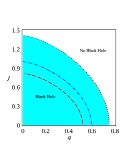
(a) $z=w=0$

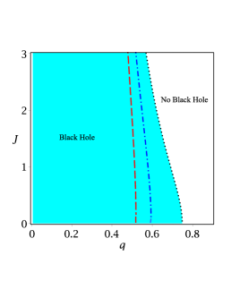
(b) $z=0$ and $w=3$

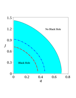
(c) $z=1$ and $w=0$

(d) $z=3$ and $w=0$

Figure 1: The admissible parameter space to have a physical solution for $m=1$, $r_{0}=1$, $\Lambda=-0.5$ (dotted line), $\Lambda=-1$ (dash-dotted line) and $\Lambda=-1.5$ (dashed line).

II.2 Singularity and Event horizon

With the exact solution in hand, we examine whether the obtained solution could be interpreted as a black hole. The interpretation of solution as a (singular) black hole has two criteria: I) Presence of singularity, II) Existence of an event horizon covering the singularity. In order to look for the singularity, we use the Kretschmann scalar as

$$K = f^{\prime\prime^{2}}+\left(\frac{3zf^{\prime}}{r}+\frac{z\left(z-2\right)f}{r^{2}}-\frac{3J^{2}\left(\frac{r}{r_{0}}\right)^{2w-z}\left(w-2\right)^{2}}{4r^{2}}\right)f^{\prime\prime}+$$ (8)

$$\frac{(\frac{9z^{2}}{4}+2)}{r^{2}}f^{\prime^{2}}+\left(\frac{3\left(z^{2}-2z+\frac{4}{3}\right)zf}{2r^{3}}-\frac{J^{2}\left(\frac{r}{r_{0}}\right)^{2w-z}\left(w-2\right)^{2}\left(\frac{9z}{4}-1\right)}{2r^{5}}\right)f^{\prime}+$$

$$\frac{z^{2}\left(\frac{z^{2}}{4}-z+2\right)}{r^{4}}f^{2}-\frac{J^{2}\left(\frac{r}{r_{0}}\right)^{2w-z}\left(w-2\right)^{2}\left[z^{2}-z\left(w+2\right)+w^{2}\right]}{2r^{6}}f+\frac{11J^{2}\left(\frac{r}{r_{0}}\right)^{4w-2z}\left(w-2\right)^{4}}{64r^{8}}.$$

Inserting the metric function $f(r)$ into Eq. (8), one finds

$$K = \Upsilon_{1}r^{2(w-z-4)}+(\Upsilon_{2}r^{\gamma}+\Upsilon_{3}r^{\gamma+\delta+2}+\Upsilon_{4}r^{\delta})r^{2w-2.5z-7}$$

$$+\left[(\Upsilon_{5}r^{\gamma+2}+\Upsilon_{6})r^{\gamma+\delta}+(\Upsilon_{7}r^{2\gamma+4}+\Upsilon_{8}r^{\gamma+2}+\Upsilon_{9})r^{2\delta}+\Upsilon_{10}r^{2\gamma}\right]r^{-3(z+2)},$$

where $\Upsilon_{i}$’s are functions of $z$, $w$, $J$, $r_{0}$, $\Lambda$, $m$ and $q$. According to our analysis, the scalar curvature diverges in the limit of $r\rightarrow 0$ which confirms that there is a curvature singularity at $r=0$.

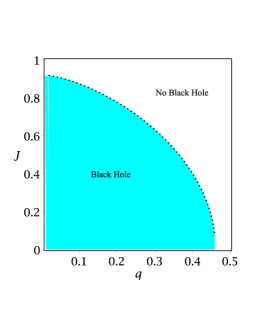
(a) $z=1$ and $w=0$

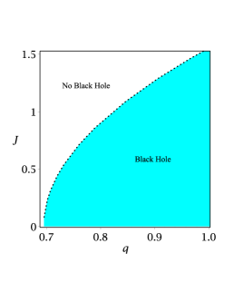
(b) $z=1$ and $w=1$

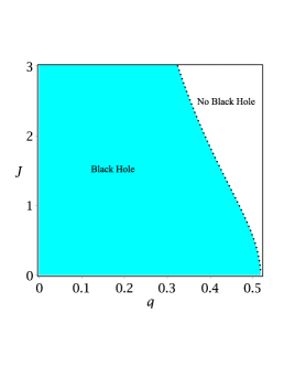
(c) $z=1$ and $w=3$

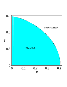
(d) $z=2$ and $w=0$

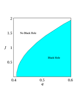
(e) $z=2$ and $w=1$

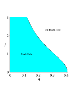
(f) $z=2$ and $w=3$

Figure 2: The admissible parameter space to have a physical solution for $m=1$, $r_{0}=1$ and $\Lambda=-1$.

Now, we require to investigate the second condition (existence of a horizon(s)). Strictly speaking, roots of the metric function, $g^{rr}=f(r)$, are where black hole’s horizons are. The absence of a root for the metric function indicates that the solution is not a black hole but a naked singularity. Due to the fact that the metric function goes to $+\infty$ for spatial infinity and also near the origin, one can find that such a function has a minimum ($r_{min}$). Depending the sign of $f(r_{min})$, one may find a black hole with two horizons ($f(r_{min})<0$), an extreme black hole ($f(r_{min})=0$) or naked singularity ($f(r_{min})>0$). We examine the condition of extreme BH by studying the following criteria

$$f(r_{min})=0=f^{\prime}(r_{min}).$$ (9)

Equation (9) shows that the metric function has one degenerate horizon at $r_{min}$ which corresponds to the radius of extremal black holes (the coincidence of the inner and outer BH horizons). Solving these two equations, simultaneously, leads to

$$q = \left(\frac{\left[(2w-z-4)\Lambda r_{min}^{\gamma+2}+m(\gamma+2w-z-2)\right]r_{min}^{\delta}2^{\frac{1}{4}}}{r_{min}^{\gamma}\left(2w-z-2+\delta\right)}\right)^{\frac{2}{3}},$$ (10)

$$J = \left(\frac{8\left(m(\gamma-\delta)-\Lambda(\delta+2)r_{min}^{\gamma+2}\right)\left(w(z+6)-2-4w^{2}\right)}{r_{min}^{\gamma-2}\left(2w-z-2+\delta\right)\left(w-2\right)^{2}\left(\frac{r_{min}}{r_{0}}\right)^{2w-z}}\right)^{\frac{1}{2}}.$$

The resultant curve provides a lower bound for the existence of the black hole, and is depicted in Fig. 1 see dotted, dash-dotted and dashed lines and Fig. 2 by the dotted line, denoting the extremal limit. Below this line, black holes (with two horizons) are present, whereas no black hole exists above it. As it was observed, the second condition for the existence of roots (horizons) for the metric function can be satisfied. In other words, the curvature singularity can be covered by an event horizon. So, the obtained solution can be interpreted as a black hole solution.

A significant point regarding these figures is that the admissible parameter space is highly affected by values of the exponent $w$. For case of $z=0$, there is no physical solution for values of $w=1$ and $w=2$. For case of $z\neq 0$, a physical solution cannot be observed for small values of the electric charge for $w=1$ (see the middle panels of Fig. 2). For the same $w$, the admissible parameter space decreases with increase of $z$ (compare left panels of these two figures with each other). Also, from Fig. 1, one can find that the cosmological constant has a decreasing effect on admissible parameter space.

II.3 Optical features

Here, we are going to investigate another geometric property of the black hole, photon orbit. To do so, we investigate the photon orbit radius of the black hole and explore the effect of the exponents $z$ and $w$ and parameters $q$ and $J$ on the radii size. At the first step, we employ the Hamilton-Jacobi equation for null curves as Carter1a

$$\frac{\partial S}{\partial\lambda}=-\frac{1}{2}g^{\mu\nu}\frac{\partial S}{\partial x^{\mu}}\frac{\partial S}{\partial x^{\nu}},$$ (11)

where $S$ and $\lambda$ denote, respectively, the Jacobi action of the photon and the affine parameter of the null geodesic. Using known constants of the motion, one can separate the Jacobi function as follows

$$S=-Et+L\phi+S_{r}(r),$$ (12)

where $E$ and $L$ are, respectively, the energy and angular momentum of the photon in the direction of rotation axis. By inserting the Jacobi action (12) into the Hamilton-Jacobi equation (11), and using also the metric components, we acquire

$$r^{2}f(r)\left(\frac{r}{r_{0}}\right)^{z}\left(\frac{dS_{r}}{dr}\right)^{2}-\frac{L^{2}J^{2}}{4r^{2}f(r)}\left(\frac{r}{r_{0}}\right)^{2w}+L^{2}\left(\frac{r}{r_{0}}\right)^{z}-\frac{E^{2}r^{2}}{f(r)}-\frac{ELJ}{f(r)}\left(\frac{r}{r_{0}}\right)^{w}=0.$$ (13)

Considering $S_{r}^{\prime}(r)=\frac{\sqrt{\mathcal{R}(r)}}{f(r)}$ and inserting it into Eq. (13), one finds

$$\mathcal{R}(r)=\frac{f(r)}{r^{2}\left(\frac{r}{r_{0}}\right)^{z}}\left(\frac{L^{2}J^{2}}{4r^{2}f(r)}\left(\frac{r}{r_{0}}\right)^{2w}-L^{2}\left(\frac{r}{r_{0}}\right)^{z}+\frac{E^{2}r^{2}}{f(r)}+\frac{ELJ}{f(r)}\left(\frac{r}{r_{0}}\right)^{w}\right).$$ (14)

Thus, the photon propagation obeys the following three equations of motion, obtained from the variation of the Jacobi action with respect to the affine parameter $\lambda$

$$\frac{dt}{d\lambda}=\frac{E}{f(r)\left(\frac{r}{r_{0}}\right)^{z}}-\frac{LJ}{2r^{2}f(r)}\left(\frac{r}{r_{0}}\right)^{w-z}$$ (15)

$$\frac{dr}{d\lambda}=\sqrt{\mathcal{R}(r)},$$ (16)

$$\frac{d\varphi}{d\lambda}=\frac{L}{r^{2}}-\frac{LJ^{2}}{4r^{4}f(r)}\left(\frac{r}{r_{0}}\right)^{2w-z}-\frac{EJ}{2r^{2}f(r)}\left(\frac{r}{r_{0}}\right)^{w-z}.$$ (17)

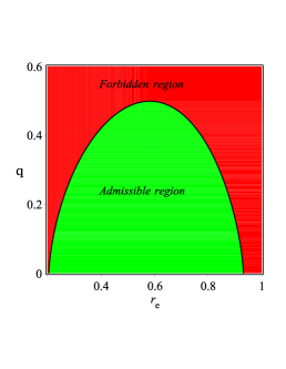
(a) $z=w=0$

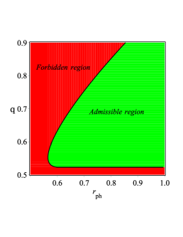
(b) $z=w=0$

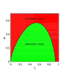
(c) $z=0$ and $w=2$

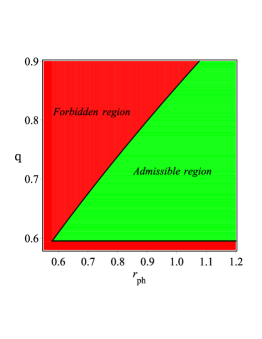
(d) $z=0$ and $w=2$

Figure 3: The admissible parameter space to have a real horizon (left panels) and a real photon sphere (right panels) for $m=1$, $\Lambda=-1$, $r_{0}=1$ and $J=0.4$.

In order to investigate the photon trajectories, one usually expresses the radial geodesics in terms of the effective potential $V_{\text{eff}}$ as

$$\left(\frac{dr}{d\lambda}\right)^{2}+V_{\text{eff}}=0,$$

with

$$V_{\text{eff}}=\frac{f(r)}{r^{2}\left(\frac{r}{r_{0}}\right)^{z}}\left(L^{2}\left(\frac{r}{r_{0}}\right)^{z}-\frac{E^{2}r^{2}}{f(r)}-\frac{ELJ}{f(r)}\left(\frac{r}{r_{0}}\right)^{w}-\frac{L^{2}J^{2}}{4r^{2}f(r)}\left(\frac{r}{r_{0}}\right)^{2w}\right).$$ (18)

Now, we are in a position to obtain the photon critical circular orbit. Therefore, the following unstable conditions should be satisfied, simultaneously

$$V_{\text{eff}}(r_{ph})=0,\quad~{}~{}~{}\frac{dV_{\text{eff}}(r_{ph})}{dr}=0,~{}~{}~{}~{}\frac{d^{2}V_{\text{eff}}(r_{ph})}{dr^{2}}<0.$$ (19)

To have an acceptable optical behavior, we need to examine the condition $r_{e}<r_{ph}$ where $r_{ph}$ and $r_{e}$ are the radius of photon orbit and event horizon radius, respectively. Figures (3) and (4) display the admissible parameter space to have a real horizon and real photon orbit. From these two figures, one can find that an acceptable optical behavior cannot be observed for $w-z<3$. In fact, by comparing the left panels with the right panels of each figure, one can see that the photon orbit radius will be imaginary in the region where the event horizon is real. In other words, in a given region one cannot observe the real horizon and real photon orbit, simultaneously.

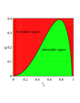
(a) $z=w=2$

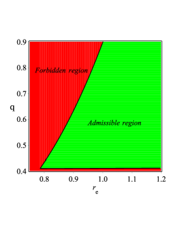
(b) $z=w=2$

(c) $z=2$ and $w=4$

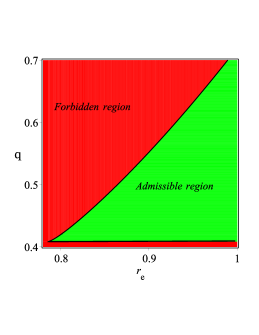
(d) $z=2$ and $w=4$

Figure 4: The admissible parameter space to have a real horizon (left panels) and a real photon sphere (right panels) for $m=1$, $\Lambda=-1$, $r_{0}=1$ and $J=0.5$.

As was already mentioned, in order to have an acceptable optical result, the condition $w-z\geq 3$ should be satisfied which is quite evident in the tables 1-3. Since relation (19) leads to a complicated equation, it is not possible to solve the equation analytically. Thus, we employ numerical methods to obtain the radius of photon orbit. In this regard, several values of the event horizon and the photon orbit radius are listed in tables 1 ($z=0$), 2 ($z=1$), and 3 ($z=2$). According to these tables, only for limited regions of the electric charge and cosmological constant, one can observe acceptable optical results. As one can see, the increase of $q$ and $|\Lambda|$ leads to an imaginary event horizon which is not a physical consequence. From these three tables, it can also be seen that the electric charge, angular momentum and the absolute value of the cosmological constant have decreasing effects on the event horizon and the radius of photon orbit. Taking a close look at the tables, one can notice that the effect of parameter $r_{0}$ is opposite of that of electric charge and angular momentum. Studying the effect of the exponent $w$ shows that increasing this parameter leads to increasing (decreasing) the event horizon (photon orbit). Comparing these three tables to each other, one can examine the effect of exponent $z$. Our analysis shows that as the parameter $z$ increases the size of the event horizon and photon orbit radius increase.

Table 1: The event horizon ($r_{e}$)and photon sphere radius ($r_{ph}$) for the variation of $q$, $J$, $r_{0}$, $w$ and $\Lambda$ for $m=1$ and $z=0$.

$q$	$0.3$	$0.4$	$0.5$	$0.6$
$r_{e}$ ($\Lambda=-1$, $J=0.4$, $r_{0}=1$, $w=3$)	$0.9216$	$0.8684$	$0.7890$	$0.57+0.05I$
$r_{ph}$ ($\Lambda=-1$, $J=0.4$, $r_{0}=1$, $w=3$)	$1.7455$	$1.6989$	$1.6385$	$1.5576$
$r_{ph}>r_{e}$	✓	✓	✓	$\times$
$J$	$0.3$	$0.4$	$0.5$	$0.6$
$r_{e}$ ($\Lambda=-1$, $q=0.3$, $r_{0}=1$, $w=3$)	$0.9217$	$0.9216$	$0.9213$	$0.9210$
$r_{ph}$ ($\Lambda=-1$, $q=0.3$, $r_{0}=1$, $w=3$)	$1.9067$	$1.7455$	$1.6325$	$1.5474$
$r_{ph}>r_{e}$	✓	✓	✓	✓
$r_{0}$	$0.7$	$0.9$	$1$	$1.1$
$r_{e}$ ($\Lambda=-1$, $q=0.3$, $J=0.4$, $w=3$)	$0.9204$	$0.9212$	$0.9216$	$0.9217$
$r_{ph}$ ($\Lambda=-1$, $q=0.3$, $J=0.4$, $w=3$)	$1.4354$	$1.5883$	$1.7455$	$1.9057$
$r_{ph}>r_{e}$	✓	✓	✓	✓
$\Lambda$	$-0.5$	$-0.8$	$-1$	$-1.2$
$r_{e}$ ($r_{0}=1$, $q=0.3$, $J=0.4$, $w=3$)	$1.3367$	$1.0404$	$0.9216$	$0.83+0.06I$
$r_{ph}$ ($r_{0}=1$, $q=0.3$, $J=0.4$, $w=3$)	$2.0506$	$1.8348$	$1.7455$	$1.6777$
$r_{ph}>r_{e}$	✓	✓	✓	$\times$
$w$	$4$	$5$	$6$	$7$
$r_{e}$ ($r_{0}=1$, $q=0.2$, $J=0.4$, $\Lambda=-1.5$)	$0.77572$	$0.77576$	$0.77581$	$0.77584$
$r_{ph}$ ($r_{0}=1$, $q=0.2$, $J=0.4$, $\Lambda=-1.5$)	$1.2488$	$1.1189$	$1.0566$	$1.0213$
$r_{ph}>r_{e}$	✓	✓	✓	✓

Table 2: The event horizon ($r_{e}$) and photon sphere radius ($r_{ph}$) for the variation of $q$, $J$, $r_{0}$, $w$ and $\Lambda$ for $m=1$ and $z=1$.

$q$	$0.3$	$0.35$	$0.4$	$0.45$
$r_{e}$ ($\Lambda=-1$, $J=0.5$, $r_{0}=1$, $w=4$)	$0.9216$	$0.8932$	$0.8588$	$0.72+0.06I$
$r_{ph}$ ($\Lambda=-1$, $J=0.5$, $r_{0}=1$, $w=4$)	$1.5012$	$1.4898$	$1.4768$	$1.4552$
$r_{ph}>r_{e}$	✓	✓	✓	$\times$
$J$	$0.2$	$0.4$	$0.6$	$0.8$
$r_{e}$ ($\Lambda=-1$, $q=0.4$, $r_{0}=1$, $w=4$)	$0.8564$	$0.8540$	$0.8530$	$0.8515$
$r_{ph}$ ($\Lambda=-1$, $q=0.4$, $r_{0}=1$, $w=4$)	$2.2107$	$1.6150$	$1.3783$	$1.2453$
$r_{ph}>r_{e}$	✓	✓	✓	✓
$r_{0}$	$0.8$	$1$	$1.2$	$1.3$
$r_{e}$ ($\Lambda=-1$, $q=0.4$, $J=0.5$, $w=4$)	$0.8487$	$0.8588$	$0.8597$	$0.8599$
$r_{ph}$ ($\Lambda=-1$, $q=0.4$, $J=0.5$, $w=4$)	$1.1135$	$1.4768$	$1.5482$	$2.1824$
$r_{ph}>r_{e}$	✓	✓	✓	✓
$\Lambda$	$-0.5$	$-0.8$	$-1$	$-1.5$
$r_{e}$ ($r_{0}=1$, $q=0.4$, $J=0.5$, $w=4$)	$1.2808$	$0.9879$	$0.8588$	$0.61+0.09I$
$r_{ph}$ ($r_{0}=1$, $q=0.4$, $J=0.5$, $w=4$)	$1.6002$	$1.4973$	$1.4768$	$1.4681$
$r_{ph}>r_{e}$	✓	✓	✓	$\times$
$w$	$5$	$6$	$7$	$8$
$r_{e}$ ($r_{0}=1$, $q=0.2$, $J=0.4$, $\Lambda=-1.5$)	$0.78831$	$0.78844$	$0.78849$	$0.78852$
$r_{ph}$ ($r_{0}=1$, $q=0.2$, $J=0.4$, $\Lambda=-1.5$)	$1.2809$	$1.1480$	$1.0831$	$1.0455$
$r_{ph}>r_{e}$	✓	✓	✓	✓

Table 3: The event horizon ($r_{e}$) and photon sphere radius ($r_{ph}$) for the variation of $q$, $J$, $r_{0}$, $w$ and $\Lambda$ for $m=1$ and $z=2$.

$q$	$0.2$	$0.3$	$0.4$	$0.5$
$r_{e}$ ($\Lambda=-1$, $J=0.5$, $r_{0}=1$, $w=5$)	$0.9640$	$0.9248$	$0.8281$	$0.81+0.15I$
$r_{ph}$ ($\Lambda=-1$, $J=0.5$, $r_{0}=1$, $w=5$)	$1.4011$	$1.3891$	$1.3733$	$1.3525$
$r_{ph}>r_{e}$	✓	✓	✓	$\times$
$J$	$0.2$	$0.4$	$0.6$	$0.8$
$r_{e}$ ($\Lambda=-1$, $q=0.4$, $r_{0}=1$, $w=5$)	$0.8302$	$0.8290$	$0.8270$	$0.8257$
$r_{ph}$ ($\Lambda=-1$, $q=0.4$, $r_{0}=1$, $w=5$)	$1.9762$	$1.4922$	$1.2868$	$1.2202$
$r_{ph}>r_{e}$	✓	✓	✓	✓
$r_{0}$	$0.9$	$1$	$1.1$	$1.2$
$r_{e}$ ($\Lambda=-1$, $q=0.4$, $J=0.5$, $w=5$)	$0.8248$	$0.8281$	$0.8290$	$0.8300$
$r_{ph}$ ($\Lambda=-1$, $q=0.4$, $J=0.5$, $w=5$)	$1.1836$	$1.3733$	$1.5908$	$1.8348$
$r_{ph}>r_{e}$	✓	✓	✓	✓
$\Lambda$	$-0.5$	$-0.8$	$-1$	$-1.1$
$r_{e}$ ($r_{0}=1$, $q=0.4$, $J=0.5$, $w=5$)	$0.9872$	$0.8417$	$0.8281$	$0.76+0.07I$
$r_{ph}$ ($r_{0}=1$, $q=0.4$, $J=0.5$, $w=5$)	$1.4472$	$1.3738$	$1.3733$	$1.3726$
$r_{ph}>r_{e}$	✓	✓	✓	$\times$
$w$	$6$	$7$	$8$	$9$
$r_{e}$ ($r_{0}=1$, $q=0.2$, $J=0.4$, $\Lambda=-1.5$)	$0.81788$	$0.81794$	$0.81799$	$0.81800$
$r_{ph}$ ($r_{0}=1$, $q=0.2$, $J=0.4$, $\Lambda=-1.5$)	$1.2768$	$1.1616$	$1.1013$	$1.0649$
$r_{ph}>r_{e}$	✓	✓	✓	✓

II.4 Energy emission rate

Now, we are interested in studying the effect of the black hole parameters on the emission of particles around the black hole. It has been known that at very high energies, the absorption cross-section for black holes oscillates around a limiting constant value $\sigma_{lim}$ which is defined in the following form for an arbitrary spacetime dimension Wei:2013

$$\sigma_{lim}=\frac{\pi^{\frac{d-2}{2}}b_{c}^{d-2}}{\Gamma(\frac{d}{2})},$$ (20)

where the critical impact parameter $b_{c}$ is given by

$$b_{c}=\frac{r_{ph}}{\sqrt{f(r_{ph})}}.$$ (21)

The energy emission rate for three-dimensional spacetime is obtained as Decanini

$$\frac{d^{2}E(\omega)}{dtd\omega}=\frac{4\pi^{2}\omega^{2}b_{c}}{e^{\frac{\omega}{T}}-1},$$ (22)

where $\omega$ is the emission frequency and $T$ is the Hawking temperature. For the corresponding black hole, the Hawking temperature is given by

$$T=\frac{\kappa}{2\pi}=\frac{f^{\prime}(r)}{4\pi}\left(\frac{r}{r_{0}}\right)^{\frac{z}{2}}\Bigg{|}_{r=r_{e}},$$ (23)

in which $\kappa$ is the surface gravity. Using Eqs. (23) and (5), one can find

$$T=\frac{\left(\frac{r_{e}}{r_{0}}\right)^{\frac{z}{2}}}{4\pi}\left(-\frac{A_{1}\left(w-2\right)^{2}J^{2}\left(\frac{r_{e}}{r_{0}}\right)^{2w-z}}{32A_{2}r_{e}^{3}}-\Lambda\left(\gamma+2\right)r_{e}-\frac{2^{-\frac{1}{4}}q^{\frac{3}{2}}\left(\delta-\gamma\right)}{r_{e}^{\gamma+1}}\right),$$ (24)

where

$$A_{1} = 2\delta-2\gamma-8w+z+6,$$ (25)

$$A_{2} = 2-zw-6w+4w^{2},$$

To study the impact of black hole parameters on the energy emission rate, we have plotted Fig. 5. Figure 5(a) illustrates the influence of the electric charge on the emission rate of a Lifshitz rotating black hole. As it is clear, there exists a peak of the energy emission rate for the black hole which shifts to the low frequency with the increase of $q$. From this figure, one can also find that this parameter has a decreasing contribution to the energy emission rate. This reveals the fact that the evaporation process would be slow for a black hole located in a powerful electric field. The effect of the angular momentum on the emission rate is depicted in Fig. 5(b), indicating that the impact of this parameter is opposite of that of the electric charge. Studying the impact of parameter $r_{0}$ and cosmological constant, we observe that both parameters have a decreasing effect on this optical quantity similar to the electric charge (see Figs. 5(c) and 5(d)). This reveals the fact that as the effect of these two parameters get weak the energy emission rate becomes significant. To study the effects of two exponents, we plot Figs. 5(e) and 5(f). From Fig. 5(e), it is clear that the parameter $w$ has an increasing contribution to the energy emission rate, while the effect of the exponent $z$ is to decrease it (see Fig. 5(f)). From what was expressed, one can find that the black hole has a longer lifetime when it rotates slowly or when it is located in a high curvature background or a powerful electric field.

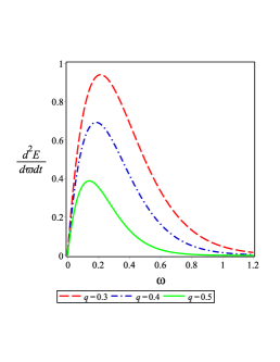
(a) $z=0$, $w=3$, $J=0.4$, $r_{0}=1$, $\Lambda=-1$

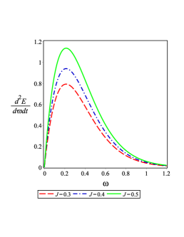
(b) $z=0$, $w=3$, $q=0.3$, $r_{0}=1$, $\Lambda=-1$

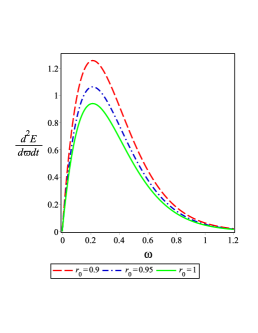
(c) $z=0$, $w=3$, $J=0.4$, $q=0.3$, $\Lambda=-1$

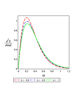
(d) $z=0$, $w=3$, $J=0.4$, $q=0.3$, $r_{0}=1$

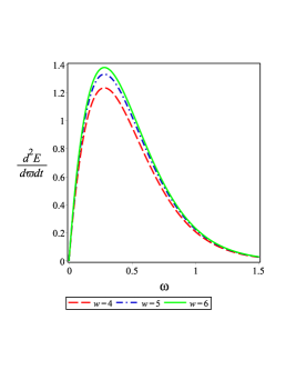
(e) $z=0$, $q=0.3$, $J=0.4$, $r_{0}=1$, $\Lambda=-1$

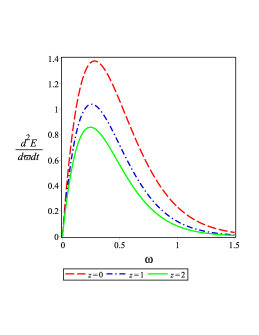
(f) $w=6$, $J=0.4$, $q=0.2$ ,$r_{0}=1$, $\Lambda=-1.5$

Figure 5: Energy emission rate for the corresponding black hole with $m=1$ and different values of black hole parameters.

III Thermodynamic properties

In this section, we would like to study the thermodynamic structure of the system. We first calculate the conserved and thermodynamics quantities of the black hole solution and examine the first law of thermodynamics. Then, we investigate phase transition and thermal stability of the black hole in the context of the canonical ensemble by calculating the heat capacity. We also examine the effects of the black hole parameters on phase transition and stability of the system and show that a certain relation between the exponents $z$ and $w$ should be satisfied in order to have a phase transition. We investigate the possibility of the existence of van der Waals-like phase transition and critical behavior for the solutions, and determine critical values. Finally, we construct a heat engine by taking into account this black hole as the working substance, and obtain the heat engine efficiency. Comparing the engine efficiency with Carnot efficiency, we investigate the criteria of having a consistent thermodynamic second law.

III.1 Thermodynamic quantities and the first law

In this subsection, we obtain the thermodynamical quantities of the solutions and check the validity of the first law of black hole thermodynamics. Before we go on, we introduce a new notion for our solutions. We consider the negative branch of cosmological constant to be a thermodynamical quantity known as pressure. Considering the cosmological constant as a thermodynamical pressure and its conjugate quantity as a thermodynamical volume leads to a new insight into thermodynamical structure of the black holes, called extended phase space thermodynamics. From now on, we replace the cosmological constant with the pressure using the following relation Kubiznak:2012

$$\Lambda = -8\pi P$$

The finite mass is the first quantity that we would like to calculate. In the non-extended phase space (the cosmological constant is not allowed to vary), the total mass of the black holes is depicted as internal energy. Considering the variable cosmological constant, the role of the mass is changed to enthalpy. There are several methods for calculating the mass. Here, to calculate this property, we use ADM (Arnowitt-Deser-Misner) approach which yields

$$M=\frac{m}{16\pi}r_{0}^{-\gamma}.$$ (26)

Evaluating the metric function on horizon $(f(r=r_{e})=0)$ and solving it with respect to geometrical mass result into the following relation for total mass of the black hole

$$M=\left(\frac{\left(w-2\right)^{2}\left(\frac{r_{e}}{r_{0}}\right)^{2w-z}}{128\pi A_{2}r_{e}^{2}}J^{2}+\frac{r_{e}^{2}P}{2}+\frac{2^{-\frac{1}{4}}q^{\frac{3}{2}}}{16\pi r_{e}^{\delta}}\right)\left(\frac{r_{e}}{r_{0}}\right)^{\gamma}.$$ (27)

The temperature of the black hole has already been obtained from Eq. (24). Replacing cosmological constant with pressure, it can be rewritten as

$$T=\frac{\left(\frac{r_{e}}{r_{0}}\right)^{\frac{z}{2}}}{4\pi}\left(-\frac{A_{1}\left(w-2\right)^{2}J^{2}\left(\frac{r_{e}}{r_{0}}\right)^{2w-z}}{32A_{2}r_{e}^{3}}+8\pi P\left(\gamma+2\right)r_{e}-\frac{2^{-\frac{1}{4}}q^{\frac{3}{2}}\left(\delta-\gamma\right)}{r_{e}^{\gamma+1}}\right).$$ (28)

As the next step, we calculate the entropy of the black hole. The method for obtaining the entropy of black holes depends on gravities under consideration and topological structure of the black holes. In Einsteinian black holes, without higher curvature terms, the entropy could be obtained by using the area law. But, since our solutions are obtained in a class of $F(R)$ gravity with $F_{R}=0$, we suppose the validity of the first law of thermodynamics to calculate the entropy as

$$\delta S=\frac{1}{T}\delta M,$$ (29)

yielding

$$S=\frac{\left(4+2\delta-\gamma\right)r_{e}\left(\frac{r_{e}}{r_{0}}\right)^{\gamma-\frac{z}{2}}}{24}.$$ (30)

As we see, entropy depends only on the exponent $z$ and there is no direct contributions of matter field. Besides, using the concept of enthalpy, one can obtain the volume of these black holes as

$$V=\left(\frac{\partial H}{\partial P}\right)\Bigg{|}_{S,Q,J}=\frac{r_{e}^{2}\left(\frac{r_{e}}{r_{0}}\right)^{\gamma}}{2}.$$ (31)

Evidently, there is a direct relationship between the total volume of the black holes and the horizon radius, indicating that one can use the horizon radius instead of using volume in calculations.

The total electric charge of the black hole can be obtained from the power Maxwell nonlinear electrodynamics as

$$Q=\frac{3\sqrt{q}2^{\frac{3}{4}}}{32\pi},$$ (32)

and the electric potential is determined as

$$U=r_{e}^{-\delta}q\left(\frac{r_{e}}{r_{0}}\right)^{\gamma}.$$ (33)

To obtain the angular velocity, we take advantage of the standard equation as

$$\Omega=-\frac{g_{t\varphi}}{g_{\varphi\varphi}}=\frac{J\left(\frac{r_{e}}{r_{0}}\right)^{w}}{2r_{e}^{2}}.$$ (34)

Considering the above equation and the first law, the angular momentum can be obtained as

$$\xi=\frac{\left(\frac{r_{e}}{r_{0}}\right)^{w+\gamma-z}\left(w-2\right)^{2}}{32\pi\left(2-zw-6w+4w^{2}\right)}J.$$ (35)

It is easy to show that the first law of thermodynamics is as follows

$$dM=TdS+UdQ+VdP+\Omega d\xi,$$ (36)

Taking into account the scaling argument for our Lifshitz like solutions in the extended phase space, one can find the following Smarr relation holds

$$\gamma M=\frac{\left(4-\delta+2\gamma\right)}{3}TS+\frac{\delta}{3}QU-2PV-\frac{\left(3w-\delta-\gamma\right)}{3}\Omega\xi.$$ (37)

It is notable that for $z=w=0$, Eq. (37) reduces to that of nonlinearly charged rotating BTZ black holes in which mass term has no scaling.

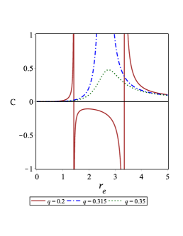
(a) $z=0.5$, $w=1.5$, $J=0.5$, $r_{0}=0.1$, $\Lambda=-0.01$

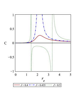
(b) $z=0.5$, $w=1.5$, $q=0.2$, $r_{0}=0.1$, $\Lambda=-0.01$

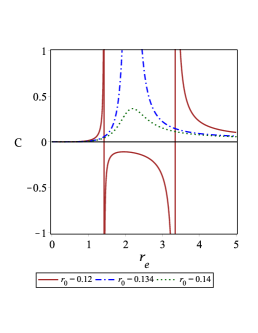
(c) $z=0.5$, $w=1.5$, $q=0.2$, $J=0.5$, $\Lambda=-0.01$

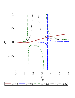
(d) $z=0.5$, $J=0.5$, $q=0.2$, $r_{0}=0.1$, $\Lambda=-0.01$

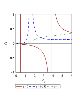
(e) $w=1$, $J=0.3$, $q=0.2$, $r_{0}=0.1$, $\Lambda=-0.01$

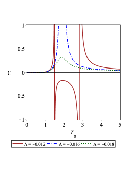
(f) $z=0.5$, $w=1.5$, $J=0.5$, $q=0.2$, $r_{0}=0.1$

Figure 6: Heat capacity versus $r_{e}$ for different values of parameters.

III.2 Thermal stability and phase transition

Heat capacity is one of the interesting thermodynamical quantities which could be used to extract two important properties of the solutions: I) Phase transition points. II) Thermal stability of the solutions. The signature of heat capacity determines the thermal stability/instability of the system. The positivity of heat capacity represents the black hole being in thermally stable state, while the opposite corresponds to thermally unstable case. As was already mentioned, the heat capacity can provide a mechanism to study the phase transition of the system. In fact, this thermodynamic quantity can be employed to investigate two distinctive points, bound and phase transition points. The bound point is where the sign of temperature is changed. In other words, the root of temperature (or heat capacity) indicates a limitation point, which separates physical solutions (positive temperature) from non-physical ones (negative temperature). The phase transition point may be related to the divergence points of $C$. Indeed, the divergencies of the heat capacity are where the system goes under phase transition. The heat capacity is given by

$$C_{P,Q,J} = T\left(\frac{\partial S}{\partial T}\right)_{P,Q,J}.$$ (38)

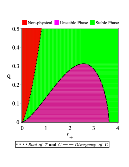
(a) $z=0.5$, $w=1.5$, $J=0.5$, $r_{0}=0.1$, $\Lambda=-0.01$

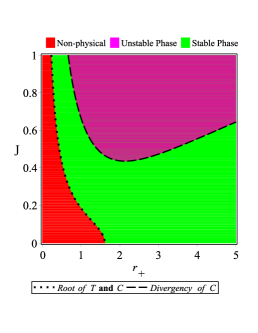
(b) $z=0.5$, $w=1.5$, $q=0.2$, $r_{0}=0.1$, $\Lambda=-0.01$

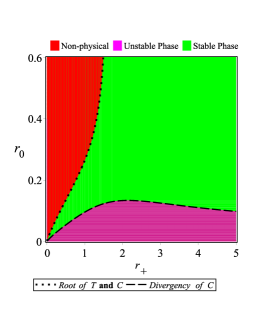
(c) $z=0.5$, $w=1.5$, $q=0.2$, $J=0.5$, $\Lambda=-0.01$

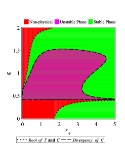
(d) $z=0.5$, $J=0.5$, $q=0.2$, $r_{0}=0.1$, $\Lambda=-0.01$

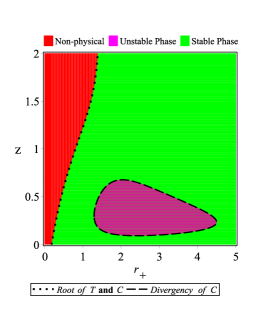
(e) $w=1.5$, $J=0.5$, $q=0.2$, $r_{0}=0.1$, $\Lambda=-0.01$

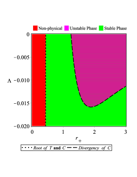
(f) $z=0.5$, $w=1.5$, $J=0.5$, $q=0.2$, $r_{0}=0.1$

Figure 7: Thermally stable and/or unstable regions of the black holes.

Employing Eqs. (30), (28) and (38), one can find

$$C_{P,Q,J} = \frac{\pi r_{e}(\frac{r_{e}}{r_{0}})^{\gamma-\frac{z}{2}}}{B_{1}+B_{2}-B_{3}}((1+\gamma-\frac{z}{2})(\gamma-2\delta-4)B_{4}),$$ (39)

in which

$$B_{1} = -3A_{1}r_{e}^{1+\delta}\left(w-2\right)^{2}(4w-z-6)\left(\frac{r_{e}}{r_{0}}\right)^{2w-z}J^{2}$$

$$B_{2} = 768\pi PA_{2}(2+z)(\gamma+2)r_{e}^{5+\delta}$$

$$B_{3} = -48A_{2}(A_{1}+8w)(\delta-\gamma)2^{-\frac{1}{4}}q^{\frac{3}{2}}r_{+}^{3}$$

$$B_{4} = \frac{A_{1}J^{2}\left(w-2\right)^{2}r_{e}^{1+\delta}}{2}\left(\frac{r_{e}}{r_{0}}\right)^{2w-z}-512r_{e}^{3}\left((\gamma+2)\pi Pr_{e}^{2+\delta}-\frac{2^{-\frac{1}{4}}q^{\frac{3}{2}}A_{2}\left(\gamma+2\right)}{32}\right).$$

The behavior of the heat capacity with respect to the horizon radius is addressed in Fig. 6. According to this figure, there are three possibilities for the heat capacity:

Case I) One root: there are two phases of small and large black holes. The small one is not physical due to the negativity of the temperature. Whereas, the large black hole phase is thermally stable.

Case II) One root and one divergency: in this case, there are three phases small, medium, and large black holes. The small black holes have negative temperatures and therefore, are not physical. The medium and large phases are separated by a divergence point. At this point, two phases of medium and large black holes are in equilibrium and go from one to the other via a critical process.

Case III) One root and two divergencies: In this case, four distinguishable phases can be observed for black holes; very small, small, medium, and large black holes. For the very small black hole phase, the temperature is negative and so this phase is not a physical one. For small and large black hole phases, heat capacity is positive and these two phases are thermally stable. Medium black hole phases which are located between two divergencies have negative heat capacity. Therefore, this phase is not physical and accessible to the black holes.

Figure 6 also displays the effects of different parameters on the heat capacity. In general, we can highlight the following effects of variation of different parameters on the heat capacity.

i) According to Fig. 6(a), there is a critical value for the electric charge where for values smaller than it, two divergencies exist for the heat capacity. These two divergencies coincide with each other for this critical value of the electric charge. For the electric charges larger than this critical value, no divergency appears in the structure of the heat capacity.

ii) Figure 6(b) shows that there is a critical value for the angular momentum as well. The only difference is that for angular momentums smaller than this critical value, no divergence point is observed.

iii) The effect of parameter $r_{0}$ is depicted in Fig. 6(c), indicating that its contribution to the heat capacity is the same as the effect of the electric charge. In other words, for the values of $r_{0}$ smaller than its critical value, two divergence points appear. While, no divergency observe for larger than the critical value.

iv) Figure 6(d) illustrates the effect of the exponent $w$ on the heat capacity. Taking a closer look at this figure, one can find that its effect is similar to the angular momentum. The difference is that for fixed parameters $q$, $J$, $z$, $r_{0}$ and $\Lambda$, there is a specific value of $w$ for which the heat capacity has only one divergency without any root (see the dashed curve of Fig. 6(d)). For this specific value, two phases exist small and large black holes. Small black holes have a negative heat capacity and are thermally unstable. Whereas, large black holes are in a stable state due to the positivity of heat capacity. For values of $w$ between this specific value and the critical value, there are two divergencies for the heat capacity.

v) To study the effect of exponent $z$ and the cosmological constant, we plot Figs. 6(e) and 6(f), indicating that their effects are similar to the electric charge.

To have a more precise picture regarding the effects of different parameters on thermal stability/instability of the solutions, we have plotted Fig. 7. As we see, by decreasing (increasing) of the electric charge, cosmological constant and parameter $r_{0}$ (angular momentum), the stability region of the system decreases. In the case of exponents, the effect of each one on the stability of the system depends on the value of the other. In fact, the value of $w$ for which the system is thermally unstable are quite dependent on the value of $z$ and vice versa.

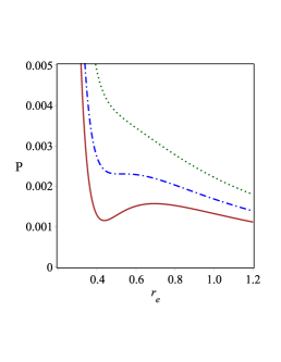
(a) $z=0.5$, $w=1.5$, $J=0.6$, $r_{0}=0.2$

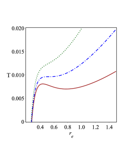
(b) $z=0.5$, $w=1.5$, $J=0.6$, $r_{0}=0.2$

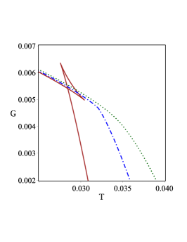
(c) $z=0.5$, $w=1.5$, $J=0.6$, $r_{0}=0.2$

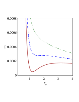
(d) $z=1$, $w=0.5$, $J=0.3$, $r_{0}=1$

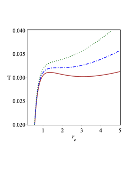
(e) $z=1$, $w=0.5$, $J=0.3$, $r_{0}=1$

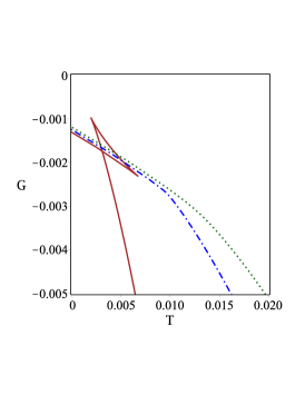
(f) $z=1$, $w=0.5$, $J=0.3$, $r_{0}=1$

Figure 8: van der Waals like phase diagrams for $q=0.1$. Left panels: $P-r_{e}$ diagram for $T<T_{c}$ (continuous line), $T=T_{c}$ (dash-dotted line), and $T>T_{c}$ (dotted line). Middle panels: $T-r_{e}$ diagram for $P<P_{c}$ (continuous line), $P=P_{c}$ (dash-dotted line), and $P>P_{c}$ (dotted line). Right panels: $G-T$ diagram for $P<P_{c}$ (continuous line), $P=P_{c}$ (dash-dotted line) and $P>P_{c}$ (dotted line).

III.3 van der Waals like behavior

Here, we look for the possibility of the existence of van der Waals-like phase transition for the black holes. We also extract critical thermodynamic quantities and analyze the effects of black hole parameters on critical values. To do so, we require to determine the equation of state which is obtained by writing down the pressure as a function of the temperature and thermodynamic volume. Since there is a direct relationship between the thermodynamic volume and the horizon radius, we use the horizon radius instead of using volume in the equation of state. From Eq. (28), the equation of state is obtained as

$$P=\frac{A_{1}J^{2}\left(w-2\right)^{2}\left(\frac{r_{e}}{r_{0}}\right)^{2w-z}}{256A_{2}\pi r_{e}^{4}}+\frac{2^{-\frac{1}{4}}q^{\frac{3}{2}}\left(\delta-\gamma\right)}{8\pi\left(\gamma+2\right)r_{e}^{\delta+2}}+\frac{T}{2r_{e}\left(\frac{r_{e}}{r_{0}}\right)^{\frac{z}{2}}\left(\gamma+2\right)}.$$ (40)

The behaviors of the pressure and temperature under variation of the event horizon radius are depicted in Fig. 8. Evidently, a van der Waals-like phase transition can be observed for these black holes by suitable choices of different parameters. Indeed, the presence of subcritical isobars in $T-r_{e}$ and isothermal diagrams in $P-r_{e}$ confirm the existence of van der Waals-like phase transition. As we know, the van der Waals fluid goes under a first order phase transition for temperatures smaller than the critical temperature $(T<T_{c})$. Whereas, at the critical temperature, its phase transition is a second-order one Kubiznak:2012 . The formation of the swallow-tail shape in the $G-T$ diagram is another evidence of the first-order (small-large) phase transition. Figures 8(c) and 8(f), confirm the first-order phase transition for our black hole solutions.

Our analysis shows that a first-order phase transition occurs for values of the exponents that satisfy the condition $x_{1}<z+w<x_{2}$. It is worth mentioning that the values of $x_{1}$ and $x_{2}$ are highly governed by the parameter $z$. Some values of $x_{1}$ and $x_{2}$ for different values of $z$ are as follows

$$z = 0.5~{}~{}\longrightarrow~{}~{}0.9<z+w<2.1$$ (41)

$$z = 1~{}~{}~{}~{}\longrightarrow~{}~{}~{}1.35<z+w<2.75$$

$$z = 1.5~{}~{}\longrightarrow~{}~{}1.8<z+w<3.35$$

$$z = 2~{}~{}~{}~{}\longrightarrow~{}~{}~{}2.3<z+w<3.85,$$

A significant point here is that if $w>z$ in the mentioned region (see the relation (41)), the Gibbs free energy is positive. Since the Gibbs free energy is obtained as $G=H-ST$, this reveals the fact that the system is energy-dominated. But for $z>w$, the Gibbs free energy is negative, indicating that the system is entropy-dominated (see Fig. 9).

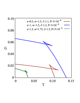
(a)

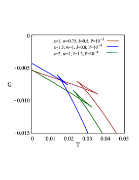
(b)

Figure 9: $G-T$ diagram for $q=0.1$ and $r_{0}=0.2$.

To obtain the critical values of thermodynamic quantities, we use the concept of the inflection point of isothermal $P-V$ diagram given by

$$\left(\frac{\partial P}{\partial r_{e}}\right)_{T}=0,\ \ \ \left(\frac{\partial^{2}P}{\partial r_{e}^{2}}\right)_{T}=0$$ (42)

It is a matter of calculation to show that the critical horizon radius (volume), temperature and pressure are given by

$$r_{c} = \frac{32wA_{2}r_{0}^{2w-z}2^{-\frac{1}{4}}q^{\frac{3}{2}}\left(\delta+2\right)\left(-2\delta+z-2\right)\left(\gamma-\delta\right)}{A_{1}J^{2}\left(w-2\right)^{2}(A_{2}-2)(2w-z-4)},$$

$$T_{c} = \frac{2^{-\frac{1}{4}}q^{\frac{3}{2}}\left(\delta+2\right)\left(\gamma-\delta\right)\left(\frac{r_{c}}{r_{0}}\right)^{\frac{z}{2}}r_{c}^{\delta-2}}{2(2+z)\pi r_{c}^{3}}+\frac{A_{1}\left(2w-z-4\right)\left(w-2\right)^{2}J^{2}\left(\frac{r_{c}}{r_{0}}\right)^{2w-\frac{z}{2}}}{32A_{2}(2+z)\pi r_{c}^{3}},$$

$$P_{c} = \frac{A_{1}J^{2}\left(w-2\right)^{2}(A_{2}-2)\left(\frac{r_{c}}{r_{0}}\right)^{2w-z}}{256\pi wA_{2}r_{c}^{4}\left(\gamma+2\right)(2+z)}-\frac{2^{-\frac{1}{4}}q^{\frac{3}{2}}\left(\gamma-\delta\right)(z-2-2\gamma)}{8(\gamma+2)(2+z)\pi r_{c}^{2+\delta}}.$$ (43)

Table 4: Critical values for the variation of $q$, $J$, $r_{0}$, $w$ and $z$.

$q$	$0.1$	$0.12$	$0.14$	$0.16$
$P_{c}$ ($z=0.5$, $w=1.5$, $J=0.6$, $r_{0}=0.2$)	$27\times 10^{-5}$	$22\times 10^{-5}$	$19\times 10^{-5}$	$17\times 10^{-5}$
$T_{c}$ ($z=0.5$, $w=1.5$, $J=0.6$, $r_{0}=0.2$)	$0.032$	$0.031$	$0.03$	$0.029$
$r_{c}$ ($z=0.5$, $w=1.5$, $J=0.6$, $r_{0}=0.2$)	$1.77$	$2.01$	$2.24$	$2.45$
$P_{c}r_{c}/T_{c}$ ($z=0.5$, $w=1.5$, $J=0.6$, $r_{0}=0.2$)	$0.0153$	$0.0148$	$0.0144$	$0.0141$
$J$	$0.5$	$0.6$	$0.7$	$0.8$
$P_{c}$ ($z=0.5$, $w=1.5$, $q=0.1$, $r_{0}=0.2$)	$14\times 10^{-5}$	$27\times 10^{-5}$	$46\times 10^{-5}$	$73\times 10^{-5}$
$T_{c}$ ($z=0.5$, $w=1.5$, $q=0.1$, $r_{0}=0.2$)	$0.021$	$0.032$	$0.045$	$0.060$
$r_{c}$ ($z=0.5$, $w=1.5$, $q=0.1$, $r_{0}=0.2$)	$2.10$	$1.77$	$1.54$	$2.45$
$P_{c}r_{c}/T_{c}$ ($z=0.5$, $w=1.5$, $q=0.1$, $r_{0}=0.2$)	$0.0147$	$0.0153$	$0.0159$	$0.0163$
$r_{0}$	$0.1$	$0.15$	$0.2$	$0.25$
$P_{c}$ ($z=0.5$, $w=1.5$, $J=0.6$, $q=0.1$)	$51\times 10^{-4}$	$93\times 10^{-5}$	$27\times 10^{-5}$	$11\times 10^{-5}$
$T_{c}$ ($z=0.5$, $w=1.5$, $J=0.6$, $q=0.1$)	$0.263$	$0.076$	$0.032$	$0.016$
$r_{c}$ ($z=0.5$, $w=1.5$, $J=0.6$, $q=0.1$)	$0.801$	$1.27$	$1.77$	$2.29$
$P_{c}r_{c}/T_{c}$ ($z=0.5$, $w=1.5$, $J=0.6$, $q=0.1$)	$0.0157$	$0.0155$	$0.0153$	$0.0152$
$w$	$1$	$1.25$	$1.5$	$1.6$
$P_{c}$ ($z=0.5$, $J=0.6$, $q=0.1$, $r_{0}=0.2$)	$0.038$	$31\times 10^{-4}$	$27\times 10^{-5}$	$19\times 10^{-6}$
$T_{c}$ ($z=0.5$, $J=0.6$, $q=0.1$, $r_{0}=0.2$)	$0.188$	$0.059$	$0.032$	$0.026$
$r_{c}$ ($z=0.5$, $J=0.6$, $q=0.1$, $r_{0}=0.2$)	$0.342$	$0.787$	$1.77$	$3.87$
$P_{c}r_{c}/T_{c}$ ($z=0.5$, $J=0.6$, $q=0.1$, $r_{0}=0.2$)	$0.0695$	$0.0423$	$0.0153$	$0.0029$
$z$	$0.5$	$1$	$1.5$	$2$
$P_{c}$ ($w=1.5$, $J=0.6$, $q=0.1$, $r_{0}=0.2$)	$27\times 10^{-5}$	$91\times 10^{-6}$	$16\times 10^{-6}$	$19\times 10^{-7}$
$T_{c}$ ($w=1.5$, $J=0.6$, $q=0.1$, $r_{0}=0.2$)	$0.032$	$0.016$	$0.007$	$0.002$
$r_{c}$ ($w=1.5$, $J=0.6$, $q=0.1$, $r_{0}=0.2$)	$1.77$	$2.07$	$2.64$	$3.45$
$P_{c}r_{c}/T_{c}$ ($w=1.5$, $J=0.6$, $q=0.1$, $r_{0}=0.2$)	$0.0153$	$0.0113$	$0.0057$	$0.0023$

Table 4 shows how critical quantities and universal critical ratio $\left(\frac{P_{c}r_{c}}{T_{c}}\right)$ change under variation of black hole parameters. From this table, one can find that as the electric charge increases, the critical pressure, temperature, and universal critical ratio decrease, whereas the critical horizon radius (volume) increases. Regarding the effect of angular momentum on the critical quantities, one can see that its effect is opposite of that of the electric charge. Studying the effects of exponents and parameter $r_{0}$ indicates that their contribution to critical values is the same as the electric charge. In other words, the critical volume is an increasing function of these three parameters, whereas the critical pressure, temperature, and universal critical ratio are decreasing functions of them.

III.4 Heat Engine

As the final step, we would like to consider the Lifshitz rotating black hole as a heat engine and discuss its efficiency.

A heat engine is a physical system that works between two hot and cold reservoirs and its main role is transferring heat from the hot reservoir to the cold one. The total mechanical work done, by the First Law, is $W=Q_{H}$ - $Q_{C}$. So, the efficiency of the heat engine is

$$\eta=\frac{W}{Q_{H}}=1-\frac{Q_{C}}{Q_{H}}.$$ (44)

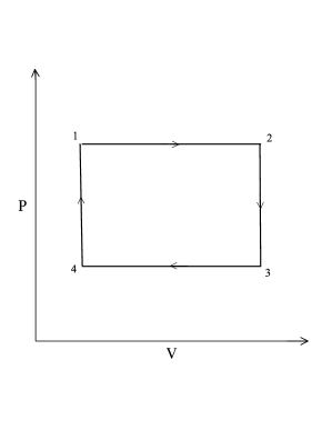
Figure 10: Our engine cycle

In order to calculate the efficiency, one may use the heat capacity. According to Eqs. (30) and (31), the entropy and thermodynamic volume are related to the horizon radius. So, these two quantities are dependent to each other for this kind of solution. This shows that the specific heat at constant volume vanishes $C_{V}=0$ which is the ”isochore equals adiabat” result CVJohnson . In this case, the specific heat at constant pressure is not zero. An explicit expression for $C_{P}$ would suggest that we can consider a rectangular cycle such as Fig. 10, involving two isobars (paths of $1\rightarrow 2$ and $3\rightarrow 4$) and two isochores/adiabats (paths of $2\rightarrow 3$ and $4\rightarrow 1$). Figure 10 shows a schematic of the proposed cycle. We can calculate the work done along the heat cycle as

$$W = \oint PdV=W_{1\longrightarrow 2}+W_{2\longrightarrow 3}+W_{3\longrightarrow 4}+W_{4\longrightarrow 1}$$ (45)

$$= W_{1\longrightarrow 2}+W_{3\longrightarrow 4}=P_{1}\left(V_{2}-V_{1}\right)+P_{4}\left(V_{4}-V_{3}\right).$$

The upper isobar will give the net inflow of heat ($Q_{H}$) as follows

$$Q_{H}=\int_{T_{1}}^{T_{2}}C_{p}\left(P_{1},T\right)dT=\int\limits_{r_{+1}}^{r_{+2}}C_{p}\left(P_{1},T\right)\frac{\partial T}{\partial r}dr=Q_{H2}-Q_{H1}.$$ (46)

Taking advantage of Eqs. (28) and (39), the input heat flow to the cycle is

$$Q_{H} = \frac{A_{1}(w-2)^{2}J^{2}(1+\gamma-\frac{z}{2})\left(2\delta+4-\gamma\right)(\frac{r_{e}}{r_{0}})^{2w-z+\gamma}}{3072\pi A_{2}\left(2w-z+\gamma-2\right)r_{e}^{2}}\Bigg{|}_{r_{e1}}^{r_{e2}}$$ (47)

$$+\frac{\left(1+\gamma-\frac{z}{2}\right)\left(\gamma-4-2\delta\right)(2^{\frac{4}{3}}q^{\frac{3}{2}}+16P_{1}\pi r_{+}^{\delta+2})(\frac{r_{e}}{r_{0}})^{\gamma}}{192r_{e}^{\delta}}\Bigg{|}_{r_{e1}}^{r_{e2}}.$$

Using Eq. (46) and (47), one can obtain the engine efficiency as

$$\eta = \frac{W}{Q_{H}}=\frac{64\pi D_{1}A_{2}r_{e2}^{2}r_{e1}^{2}}{-(D_{2}+D_{3})\left((6+z)^{2}-(2\delta-2\gamma)^{2}\right)},$$ (48)

in which

$$D_{1} = \frac{r_{e1}^{2+\gamma}-r_{e2}^{2+\gamma}}{r_{0}^{\gamma}}$$

$$D_{2} = \left(4A_{2}P_{1}\pi r_{e1}^{\delta+2}+\frac{J^{2}(w-2)^{2}r_{e1}^{2w-z+\gamma-1}}{32r_{0}^{2w-z}}+\frac{1}{4}A_{2}2^{-\frac{1}{4}}q^{\frac{3}{2}}\right)r_{e2}^{\delta}\left(\frac{r_{e1}}{r_{0}}\right)^{\gamma}$$

$$D_{3} = \left(4A_{2}P_{1}\pi r_{e2}^{\delta+2}+\frac{J^{2}(w-2)^{2}r_{e2}^{2w-z+\gamma-1}}{32r_{0}^{2w-z}}+\frac{1}{4}A_{2}2^{-\frac{1}{4}}q^{\frac{3}{2}}\right)r_{e1}^{\delta}\left(\frac{r_{e2}}{r_{0}}\right)^{\gamma}.$$

Among different classical cycles, the Carnot cycle is one of the interesting simplest cycle that can be considered. The efficiency of this cycle is the maximum efficiency of the heat engines in such a way that any higher efficiency would violate the second law of thermodynamics. To calculate the Carnot efficiency, we consider the $T_{H}$ and $T_{C}$ in our cycle to correspond to $T_{2}$ and $T_{4}$, respectively. So, this efficiency is

$$\eta_{c} = 1-\frac{T_{C}}{T_{H}}=1-\frac{X_{1}(\frac{r_{e1}}{r_{0}})^{\frac{z}{2}}}{X_{2}(\frac{r_{e2}}{r_{0}})^{\frac{z}{2}}}$$ (49)

where

$$X_{1} = -\frac{A_{1}J^{2}(w-2)^{2}(\frac{r_{e1}}{r_{0}})^{2w-z}}{32A_{2}r_{e1}^{3}}+8\pi P_{4}r_{e1}\left(\gamma+2\right)-\frac{2^{-\frac{1}{4}}q^{\frac{3}{2}}(\delta-\gamma)}{r_{e1}^{\delta+1}}$$

$$X_{2} = -\frac{A_{1}J^{2}(w-2)^{2}(\frac{r_{e2}}{r_{0}})^{2w-z}}{32A_{2}r_{e2}^{3}}+8\pi P_{4}r_{e2}\left(\gamma+2\right)-\frac{2^{-\frac{1}{4}}q^{\frac{3}{2}}(\delta-\gamma)}{r_{e2}^{\delta+1}},$$

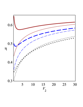
(a)

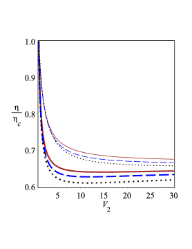
(b)

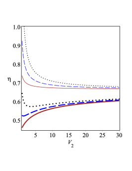
(c)

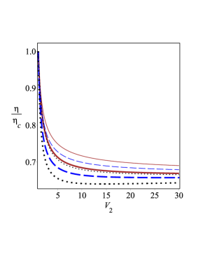
(d)

Figure 11: Variation of $\eta$ and $\frac{\eta}{\eta_{C}}$ versus $V_{2}$ for $z=0.5$, $w=1.5$, $r_{0}=0.2$, $P_{1}=0.003$, $P_{4}=0.001$ and $V_{1}=1$. Up panels: bold lines for $q=0.3$ and thin lines for $q=0$; $J=0.4$ (continues line), $J=0.5$ (dashed line) and $J=0.65$ (dotted line). Down panels: bold lines for $J=0.4$ and thin lines for $J=0$; $q=0.1$ (continues line), $q=0.2$ (dashed line) and $q=0.3$ (dotted line).

The behavior of the heat engine efficiency $\eta$ and the ratio $\frac{\eta}{\eta_{C}}$ under variation of black hole parameters is depicted in Figs. (11)-(13). In Fig. 11, we examine the influence of electric charge and angular momentum on $\eta$ and the ratio $\frac{\eta}{\eta_{C}}$ for the fixed exponents, parameter $r_{0}$ and pressures $P_{1}$, $P_{4}$. As one can check, from the up panels of Fig. 11, both $\eta$ and the ratio $\frac{\eta}{\eta_{C}}$ are decreasing functions of the angular momentum. For large values of $J$, the efficiency monotonically increases as the volume $V_{2}$ grows (see the bold dotted line of Fig. 11(a)). This means that for rapidly charged rotating black holes, the increase of volume difference between the small black hole ($V_{1}$) and larger black hole ($V_{2}$) will make the heat engine more efficient. For small angular momentum, the efficiency curve has a local minimum value, indicating that there exists a specific value of the volume $V_{2}$ at which the black hole heat engine works at the lowest efficiency (see the bold continuous line of Fig. 11(a)). In the absence of the electric charge, for all values of the angular momentum the heat engine efficiency monotonously increases with the growth of $V_{2}$ and then tends to a constant value (see thin lines of Fig. 11(a)). Taking a close look at Fig. 11(a), one can find that charged rotating black holes have a bigger efficiency than their uncharged counterparts (compare bold and thin lines). Just for large volume difference $\Delta V=V_{2}-V_{1}$, their efficiency becomes smaller compared to that of a rapidly rotating black hole (compare bold-dotted and thin-dotted lines in Fig. 11(a)).

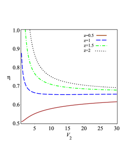
(a) $w=1.5$

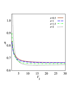
(b) $w=1.5$

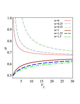
(c) $z=0.5$

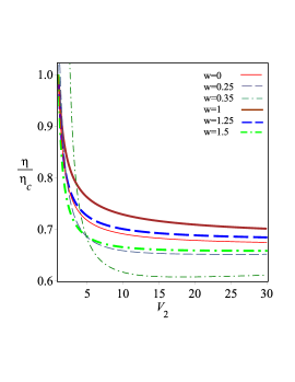
(d) $z=0.5$

Figure 12: Variation of $\eta$ and $\frac{\eta}{\eta_{C}}$ versus $V_{2}$ for $J=0.4$, $q=0.2$, $r_{0}=0.2$, $P_{1}=0.003$, $P_{4}=0.001$ and $V_{1}=1$. Up panels: for different values of $z$ parameter. Down panels: for different values of $w$ parameter.

Down panels of Fig. 11 displays the effect of the electric charge on $\eta$ and the ratio $\frac{\eta}{\eta_{C}}$. As we see, although this parameter has an increasing contribution to the efficiency, its effect is to decrease the ratio $\frac{\eta}{\eta_{C}}$. For non-rotating black holes, all curves monotonic reduce rapidly firstly, then the efficiency reaches a constant value after the certain value of volume $V_{2}$ (see thin lines of Fig. 11(c)). For slowly charged rotating black holes, the efficiency gradually increases as the volume $V_{2}$ increases and then tends to a constant value (see the bold continuous line of Fig. 11(c)). While for rapidly charged rotating black holes, the efficiency decreases to a minimum value with an increase of $V_{2}$ and then gradually grows as the volume increases more, and finally reaches a constant value in the limit of that $V_{2}$ goes to the infinity (see the bold dotted line of Fig. 11(c)). Fig. 11(c) also shows that non-rotating black holes have a bigger efficiency compared to the charged rotating black holes (compare bold lines to thin lines). Comparing Fig. 11(a) to Fig. 11(c), one can find that variation of $J$ has a stronger effect on the efficiency than the electric charge.

Figure 12 shows how $\eta$ and the ratio $\frac{\eta}{\eta_{C}}$ are affected by the exponents. According to the up panels of this figure, the exponent $z$ has an increasing (a decreasing) effect on the efficiency (the ratio $\frac{\eta}{\eta_{C}}$). For small values of $z$, the efficiency monotonically increases as the volume $V_{2}$ grows and then tends to the saturation value (see the continuous line of Fig. 12(a)). While for large values, the opposite behavior will be observed. Figure 12(c) displays the influence of the exponent $w$ on the efficiency. Our findings indicate that for $w<0.5$, the efficiency increases with the increase of $w$. While for $w>0.5$, increasing $w$ leads to the decreasing of the heat engine efficiency. Regarding the effect of this parameter on the ratio $\frac{\eta}{\eta_{C}}$, in both regions ($w<0.5$ or $w>0.5$), one finds that increasing the this parameter makes the increasing of the ratio $\frac{\eta}{\eta_{C}}$ (see Fig. 12(d)). Taking a close look at the right panels of Fig. 12, one can notice that in the region of volume $V_{2}$ near $V_{1}$ and for small (large) values of $w$ ($z$), the efficiency becomes larger than Carnot efficiency which violates the second law of thermodynamics. This shows that small (large) values of $z$ ($w$) should be considered to observe an acceptable efficiency of the system.

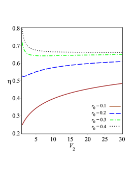
(a) $\Delta P=0.002$

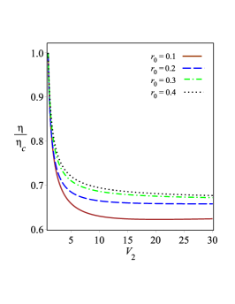
(b) $\Delta P=0.002$

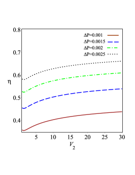
(c) $r_{0}=0.2$

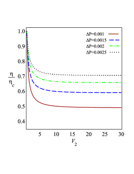
(d) $r_{0}=0.2$

Figure 13: Variation of $\eta$ and $\frac{\eta}{\eta_{C}}$ versus $V_{2}$ for $J=0.4$, $q=0.2$, $z=0.5$, $w=1.5$ and $V_{1}=1$. Up panels: for different values of $r_{0}$ parameter. Down panels: for different values of the pressure difference.

The effects of the parameter $r_{0}$ and pressure on $\eta$ and the ratio $\frac{\eta}{\eta_{C}}$ are reflected in Fig. 13. We find that the parameter $r_{0}$ has an increasing effect on both $\eta$ and $\frac{\eta}{\eta_{C}}$. For small (large) values of $r_{0}$, the efficiency gradually grows (reduces) with the increase of $V_{2}$ (see Fig. 13(a)). Regarding the pressure, down panels of Fig. 13 show that increasing the difference of pressure $\Delta P$ makes the increasing of both $\eta$ and $\frac{\eta}{\eta_{C}}$. Taking a look at right panels of Fig. 13, one can find that the second law of thermodynamics is satisfied for all values of these two parameters.

IV conclusion

In this paper, we have obtained a new Lifshitz-like rotating black hole solution in three dimensional $F(R)$ gravity. Investigating geometrical properties of the solution, we have found that this solution reduces to the charged rotating BTZ-like black hole in special limits. We also studied the optical features of the black hole and noticed that some constraints should be imposed on the exponents to have an acceptable optical behavior. Studying the impact of parameters of the model on the photon orbit radius illustrated that as the electric charge, angular momentum and absolute value of the cosmological constant increase, both event horizon and photon orbit radii decrease. Regarding the effect of exponent $z$, our analysis showed that this parameter has an increasing contribution to the horizon radii and photon orbit.

After that, we continued our analysis by investigating the energy emission rate and examining the influence of parameters on the radiation process. The results indicated that the angular momentum and exponent $z$ have an increasing contribution to the emission rate, namely, the emission of particles around the BH increases by increasing these two parameters. Regarding the role of the electric charge, cosmological constant and exponent $w$, we have found that as the effects of these parameters get stronger, the evaporation process gets slower. In other words, the lifetime of a black hole would be longer under such conditions.

As the next step, we have studied the thermodynamic properties of the system in the extended phase space thermodynamics. We calculated thermodynamic quantities of black holes and showed that these quantities satisfy the first law of thermodynamics. We also obtained the modified Smarr relation and found that regardless of the cosmological constant term, scaling other thermodynamic quantities is modified. Using heat capacity, we investigated the thermal stability of the system and showed how the parameters of the model affect the region of the stability. Moreover, we look for possible phase transitions and found that three-dimensional Lifshitz-like rotating black hole experiences the first-order/second-order phase transitions with a suitable choice of parameters.

Finally, we have considered this kind of black hole as a working substance and studied the holographic heat engine by taking a rectangle heat cycle in the $P-V$ plot. Investigating the black hole heat engine efficiency and comparing obtained results with the Carnot efficiency led to the following interesting results:

I) The angular momentum (electric charge) has a decreasing (an increasing) contribution to the efficiency of the system. For all values of these two parameters, the efficiency is always smaller than the Carnot efficiency which is consistent with the second law of thermodynamics.

II) The charged rotating black hole has a bigger (smaller) efficiency than its uncharged (non-rotating) counterpart. It is worth pointing out that for very large volume difference, the efficiency of rapidly rotating black hole becomes bigger than them.

III) The heat engine efficiency is an increasing function of the exponent $z$. For small values of this parameter, the condition $\frac{\eta}{\eta_{C}}<1$ is satisfied all the time. But for large values of $z$, this condition is violated in the region of volume $V_{2}$ near $V_{1}$. The contribution of the exponent $w$ on the efficiency is a little different. For $w<0.5$, the efficiency increases with the increase of $w$, whereas for $w>0.5$, increasing this parameter leads to the decrease of the heat engine efficiency. For $w<0.5$, the second law of thermodynamics violates for a very small volume difference, whereas for $w>0.5$ it is always preserved.

IV) Increasing the pressure difference makes the increasing the efficiency of the system. For all values of pressure, the efficiency is always smaller than the Carnot efficiency which is consistent with the second law of thermodynamics.

- (1) M. Akbar and R. G. Cai, Phys. Lett. B 635, 7 (2006).
- (2) J. C. C. de Souza and V. Faraoni, Class. Quant. Grav. 24, 3637 (2007).
- (3) G. Cognola, E. Elizalde, S. Nojiri, S. D. Odintsov, L. Sebastiani and S. Zerbini, Phys. Rev. D 77, 046009 (2008).
- (4) S. Perlmutter, et al., Astrophys. 517, 565 (1999).
- (5) A. G. Riess, et al., Astrophys. 116, 1009 (1998).
- (6) A. G. Riess, et al., Astrophys. 607,665 (2004).
- (7) R. Woodard, Lect. Notes Phys. 720, 403 (2007).
- (8) S. Capozziello, A. Troisi, Phys. Rev. D 72, 044022 (2005).
- (9) S. Capozziello, A. Stabile, A. Troisi, Phys. Rev. D 76, 104019 (2007).
- (10) A. D. Dolgov and M. Kawasaki, Phys. Lett. B 573, 1 (2003).
- (11) V. Faraoni, Phys. Rev. D 74, 104017 (2006).
- (12) P. Horava, J. High Energy Phys. 09 020 (2009).
- (13) P. Horava, Phys. Rev. D 79, 084008 (2009).
- (14) S. Kachru, X. Liu and M. Mulligan, Phys. Rev. D 78, 106005 (2008).
- (15) J. Cardy, Scaling and Renormalization in Statistical Physics (Cambridge University Press, Cambridge, 2002).
- (16) M. Banados, C. Teitelboim, J. Zanelli, Phys. Rev. Lett. 69 (1992) 1849
- (17) H. -W. Lee, Y. -S. Myung, and J. -Y. Kim, Phys. Lett. B 466, 211 (1999).
- (18) A. Larranaga, Commun. Theor. Phys. 50, 1341 (2008).
- (19) E. Witten, Three-Dimensional Gravity Revisited, [arXiv:0706.3359].
- (20) E. Witten, Adv. Theor. Math. Phys. 2, 505 (1998).
- (21) S. Carlip, Class. Quantum Gravity 22, 85 (2005).
- (22) M. A. Anacleto, F. A. Brito, and E. Passos, Phys. Lett. B 743, 184 (2015).
- (23) S. H. Hendi, B. Eslam Panah and S. Panahiyan, JHEP 05, 029 (2016).
- (24) K. C. K. Chan and R. B. Mann, Phys. Rev. D 50, 6385 (1994).
- (25) S. H. Hendi, B. Eslam Panah and S. Panahiyan, PTEP 2016, 103A02 (2016).
- (26) S. H. Hendi, S. Panahiyan, S. Upadhyay and B. Eslam Panah, Phys. Rev. D 95, 084036 (2017).
- (27) F. W. Shu, K. Lin, A. Wang, Q. Wu, JHEP 04, 056 (2014).
- (28) S. H. Hendi, R. Ramezani-Arani, E. Rahimi, Phys. Lett. B 805, 135436 (2020).
- (29) J. M. Bardeen, B. Carter, S. Hawking, Commun. Math. Phys. 31, 161 (1973).
- (30) A. Strominger, C. Vafa, Phys. Lett. B 379, 99 (1996).
- (31) X.-X. Zeng, H.-Q. Zhang, Nucl. Phys. B 959, 115162 (2020).
- (32) M. M. Caldarelli, G. Cognola, D. Klemm, Class. Quantum Grav. 17, 399 (2000).
- (33) T. Hertog, K. Maeda, Phys. Rev. D 71, 024001 (2005).
- (34) H. Lu, C. N. Pope, Q. Wen, JHEP 03, 165 (2015).
- (35) D. Kubiznak, R. B. Mann, JHEP 07, 033 (2012).
- (36) S. W. Hawking, D. N. Page, Comm. Math. Phys. 87, 577 (1983).
- (37) A. Chamblin, R. Emparan, C. Johnson, and R. Myers, Phys. Rev. D 60, 064018 (1999).
- (38) A. Chamblin, R. Emparan, C. Johnson, and R. Myers, Phys. Rev. D 60, 104026 (1999).
- (39) A. Haldar, R. Biswas, Gen. Relativ. Gravit. 50, 69 (2018).
- (40) J. X. Mo, Astrophys. Space Sci. 356, 319 (2015).
- (41) Kh. Jafarzade, J. Sadeghi, Internat. J. Modern Phys. D 26, 1750138 (2017).
- (42) R. G. Cai, L. M. Cao, L. Li, R. Q. Yang, JHEP 09, 005 (2013).
- (43) J. X. Mo, W. B. Liu, Phys. Rev. D 89, 084057 (2014).
- (44) Y. G. Miao, Z. M. Xu, Phys. Rev. D 98, 084051 (2018).
- (45) J. X. Mo, W. B. Liu, Eur. Phys. J. C 74, 2836 (2014).
- (46) S. H. Hendi, S. Panahiyan, B. Eslam Panah, Prog. Theor. Exp. Phys. 2015, 103E01 (2015).
- (47) R. Zhao, H. Zhao, M. S. Ma, L. C. Zhang, Eur. Phys. J. C 73, 2645 (2013).
- (48) M. H. Dehghani, S. Kamrani, A. Sheykhi, Phys. Rev. D 90, 104020 (2014).
- (49) J. X. Mo, G. Q. Li, Y. C. Wu, J. Cosmol. Astropart. Phys. 04, 045 (2016).
- (50) A. Ovgun, Adv. High Energy Phys. 2018, 8153721 (2018).
- (51) B. Mirza, Z. Sherkatghanad, Phys. Rev. D 90, 084006 (2014).
- (52) S. H. Hendi, B. Eslam Panah, S. Panahiyan, Class. Quantum Gravit. 33, 235007 (2016).
- (53) M. Chabab, H. El Moumni, S. Iraoui, K. Masmar, Eur. Phys. J. C 79, 342 (2019).
- (54) S. H. Hendi, S. Panahiyan, B. Eslam Panah, M. Faizal, M. Momennia, Phys. Rev. D 94, 024028 (2016).
- (55) Z. W. Feng, S. Z. Yang, Phys. Lett. B 772, 737 (2017).
- (56) S. H. Hendi, B. Eslam Panah, S. Panahiyan, Phys. Lett. B 769, 191 (2017).
- (57) G. Gibbons, R. Kallosh, B. Kol, Phys. Rev. Lett. 77, 4992 (1996).
- (58) N. Breton, Gen. Relativ. Gravit. 37, 643 (2005).
- (59) D. Kastor, S. Ray, J. Traschen, Class. Quantum Gravity 26, 195011 (2009).
- (60) S. H. Hendi, M. H. Vahidinia, Phys. Rev. D 88, 084045 (2013).
- (61) C. V. Johnson, Class. Quantum Grav. 31, 205002 (2014).
- (62) R. A. Hennigar, F. McCarthy, A. Ballon, and R. B. Mann, Class. Quantum Grav. 34, 175005 (2017).
- (63) Kh. Jafarzade, and J. Sadeghi, Int. J. Theor. Phys. 56 , 3387 (2017).
- (64) Kh. Jafarzade, and J. Sadeghi, Int. J. Mod. Phys. D 26, 1750138 (2017).
- (65) C. V. Johnson, Class. Quantum Grav. 33, 135001 (2016).
- (66) J. X. Mo , F. Liang and G. Q. Li, JHEP 03, 010 (2017).
- (67) J. Zhang, Y. Li, and H. Yu, Eur. Phys. J. C 78, 645 (2018).
- (68) S. H. Hendi, B. Eslam Panah, S. Panahiyan, H. Liu, and X. H. Meng, Phys. Lett. B 781, 40 (2018).
- (69) B. Eslam Panah, Phys. Lett. B 787, 45 (2018).
- (70) B. Carter, Phys. Rev. 174, 1559 (1968).
- (71) S. W. Wei, and Y. X. Liu, J. Cosmol. Astropart. Phys. 11, 063 (2013).
- (72) Y. Decanini, G. Esposito-Farèse, A. Folacci, Phys. Rev. D 83, 044032 (2011).