Measuring inflaton couplings via dark radiation as $\Delta N_{\rm eff}$ in CMB

Abstract

We study the production of a beyond the Standard Model (BSM) free-streaming relativistic particles which contribute to $N_{eff}$ and investigate how much the predictions for the inflationary analysis change. We consider inflaton decay as the source of this dark radiation (DR) and use the Cosmic Microwave Background (CMB) data from Planck-2018 to constrain the scenarios and identify the parameter space involving couplings and masses of the inflaton that will be within the reach of next-generation CMB experiments like spt-3g, CMB-S4, CMB-Bh$\overline{a}$rat, PICO, CMB-HD, etc. We find that if the BSM particle is produced only from the interaction with inflaton along with Standard Model (SM) relativistic particles, then its contribution to $N_{\mathrm{eff}}$ is a monotonically increasing function of the branching fraction, $B_{X}$ of the inflaton to the BSM particle $X$; Planck bound on $N_{\mathrm{eff}}$ rules out such $B_{X}\gtrsim 0.09$. Considering two different analyses of Planck+Bicep data together with other cosmological observations, $N_{\mathrm{eff}}$ is treated as a free parameter, which relaxes the constraints on scalar spectral index ($n_{s}$) and tensor-to-scalar ratio ($r$). The first analysis leads to predictions on the inflationary models like Hilltop inflation being consistent with the data. Second analysis rules out the possibility that BSM particle $X$ producing from the inflaton decay in Coleman-Weinberg Inflation or Starobinsky Inflation scenarios. To this end, we assume that SM Higgs is produced along with the BSM particle. We explore the possibilities that $X$ can be either a scalar or a fermion or a gauge boson and consider possible interactions with inflaton and find out the permissible range on the allowed parameter space Planck and those which will be within the reaches of future CMB observations.

I Introduction

For resolving the horizon problem, the flatness problem and lay the seed for structure formation in the late universe cosmic inflation Starobinsky:1980te ; Sato:1980yn ; Guth:1980zm ; Linde:1981mu ; Albrecht:1982wi ; Linde:1983gd is the leading paradigm. This period in the very early universe involves an accelerated expansion epoch during which vacuum quantum fluctuations of the gravitational and matter fields were amplified to large-scale cosmological perturbations Starobinsky:1979ty ; Mukhanov:1981xt ; Hawking:1982cz ; Starobinsky:1982ee ; Guth:1982ec ; Bardeen:1983qw , that later seeded the anisotropies as observed in Cosmic Microwave Background Radiation (CMBR) and lead to the formation of the Large Scale Structure (LSS) of our Universe.

What we observe in CMBR can be accounted for in a minimal setup, where inflation is driven typically by a single scalar field $\phi$ with canonical kinetic term, minimally coupled to gravity, and evolving in a flat potential $V(\phi)$ in the slow-roll regime. Since particle physics beyond the electroweak scale remains elusive and given that inflation can proceed at energy scales as large as $10^{16}\,\text{GeV}$, even within this class of models, hundreds of inflationary scenarios have been proposed to match with the latest sophisticated measurements of CMB Ade:2013sjv ; Adam:2015rua ; Array:2015xqh ; Ade:2015lrj . A systematic Bayesian analysis reveals that one-third of them can now be considered as ruled out Martin:2013tda ; Martin:2013nzq ; Vennin:2015eaa , while the vast majority of the preferred scenarios are of the plateau type, i.e., they are such that the potential $V(\phi)$ is a monotonic function that asymptotes a constant value when $\phi$ goes to infinity.

Cosmic inflation must be succeeded by a period during which the inflaton’s energy must be transferred to relativistic SM particles, resulting in the formation of a hot universe consistent with present observations. The extremely adiabatic reheating epoch is important since it produces all matter in the cosmos as well as the relativistic SM fluid that raises the temperature of the universe. During this epoch, the standard picture is that the inflaton field vibrates coherently around the minimum of its potential, producing SM particles as well as viable BSM particles via gravitational interactions or other couplings that maybe available in the theory. This BSM particle may contribute to the dark matter sector or stay relativistic, contributing to dark radiation (DR). If they contribute to DR, they may influence the expansion rate of the universe (and thus the measured value of Hubble parameter), CMB anisotropy Menegoni:2012tq , and the perturbation for large scale structure-formation in the universe Archidiacono:2011gq . Moreover, DR can also be produced from the decays of massive particles Hasenkamp:2012ii , $U(1)$ gauge field which is singlet under SM Ackerman:2008kmp . There are several proposed particles as viable candidate from DR e.g., light sterile neutrino Archidiacono:2016kkh ; Archidiacono:2014apa , neutralino Bae:2013hma , axions DiValentino:2013qma ; DEramo:2018vss , Goldstone bosons Weinberg:2013kea , early dark energy Calabrese:2011hg .

The predictions of inflationary models, such as $n_{s}$ and $r$, are solely determined by the parameters of the models and are independent of the presence of DR in the universe. However, the presence of extra relativistic species in the standard cosmology does have an impact on the selection of inflationary models. In particular, single-field slow-roll models, which are known to produce high values of the scalar spectral index in standard cosmology may be more favorable in the presence of extra relativistic species. Upcoming CMB experiments e.g. spt-3g, CMB Stage IV (CMB-S4), CMB-Bh$\overline{a}$rat, PICO, and CMB-HD, all of which are highly sensitive to the additional relativistic degrees of freedom, are expected to offer more precise information on the extra relativistic BSM particles present along with CMB photons. Gaining this information is significant for developing a more complete and accurate theory of the physics of the early universe, including inflationary epoch followed by reheating era, and has important impacts on understanding the underlying physics of the thermal history, Hubble expansion rate, and other cosmological phenomena of the later universe.

In this work, we make the assumption that the DR is created during the reheating epoch as a relativistic non-thermal BSM particle together with relativistic SM particles, and that the inflaton is the only source of this radiation. We then apply the bounds on DR from the CMB to the branching fraction for the production of extra relativistic BSM particle. Next, we explore the possibilities of the extra DR particle being a fermion, boson, or gauge boson and consider the possible leading-order interactions. Utilizing the present bound from current CMB observations and prospective sensitivity reaches on DR from future CMB experiments, we proceed to identify the parameter space that involves the inflaton mass, as well as the couplings between the inflaton and both the visible sector and the DR particle.

The paper is organized as follows: we begin with a discussion of $N_{\mathrm{eff}}$ and $\Delta N_{\mathrm{eff}}$ in Section II. In Section III, we consider $n_{s}-r$ predictions from four disparate inflationary models and review whether they can be ruled out as viable inflationary models by the bound from Planck2015+Bicep2 data while $N_{\mathrm{eff}}$ is allowed to vary from its standard value. In Section IV, we consider the production of a BSM particle during the reheating era, which adds an extra relativistic degree to CMB. We also explore the connection between branching fraction for the production of that BSM particle and $\Delta N_{\mathrm{eff}}$. In Section V, we look at probable interactions between the inflaton and the BSM particle, as well as the permitted parameter space for the couplings related to the bound on $N_{\mathrm{eff}}$ from CMB. In Section VI, we summarize the findings.

In this work, we use the natural unit with $\hbar=c=k_{B}=1$, such that the reduced Planck mass is $M_{P}\simeq 2.4\times 10^{18}\,\text{GeV}$. Furthermore, we also assume that the signature of the space-time metric is $(+,-,-,-)$.

II Effective number of relativistic degrees of freedom

Since the temperature of the CMB photons is a well-known quantity, the current total energy density of the relativistic species of the universe, $\rho_{{\rm rad},{\rm tot}}$, can be expressed in terms of the energy density of SM photon, $\rho_{\gamma}$, as Archidiacono:2011gq ; Mangano:2001iu ; ParticleDataGroup:2020ssz ; Boehm:2012gr ; Paul:2018njm ; Hasenkamp:2012ii ; Tram:2016rcw

$$\rho_{{\rm rad},{\rm tot}} =\rho_{\gamma}\quantity[1+\frac{7}{8}\left(\frac{4}{11}\right)^{4/3}N_{\mathrm{eff}}]\,,$$ (1)

where $N_{\mathrm{eff}}$, also known as effective number of relativistic degrees of freedom Archidiacono:2011gq , parameterizes the contribution from non-photon relativistic particles, such as SM cosmic neutrinos. There are three left-handed light cosmic neutrinos, and they were in thermal equilibrium with the SM relativistic particles in the hot early universe. When the temperature of the universe drops to $800\,\text{keV}$, neutrinos decouple from the SM photons just before the electron-positron annihilation. If we assume neutrinos decouple instantly, their contribution to $N_{\mathrm{eff}}$ is expected to be $3$. However, if we consider noninstantaneous decoupling of cosmic neutrinos Husdal:2016haj , QED correction Mangano:2001iu , and three-neutrino flavor oscillations on the neutrino decoupling phase Mangano:2005cc (see also Bennett:2019ewm ), then, neutrinos get partially heated during electron-positron decoupling from photon, resulting in slightly higher temperature of neutrinos. This leads to EscuderoAbenza:2020cmq (see also deSalas:2016ztq )

$${N_{\mathrm{eff}}}_{,\text{SM}}=3.046\,.$$ (2)

Any measured value higher than Eq. (2) suggests the possibility of the existence of any relativistic BSM particle. The contribution of the BSM particle in $N_{\mathrm{eff}}$ is expressed as ParticleDataGroup:2020ssz ; Abazajian:2019eic ; Abazajian:2019oqj ; Luo:2020sho

$$\Delta N_{\mathrm{eff}} =N_{\mathrm{eff}}-{N_{\mathrm{eff}}}_{,\text{SM}}\,.$$ (3)

Current bounds on and prospective future sensitivity reaches on $\Delta N_{\mathrm{eff}}$ from that will be within the reach of future CMB measurements are mentioned in Table 1.

Table 1: Bounds on $N_{\mathrm{eff}}$ (or $\Delta N_{\mathrm{eff}}$) from present CMB observations and prospective future reaches of $N_{\mathrm{eff}}$ (or $\Delta N_{\mathrm{eff}}$) that upcoming CMB experiments may be able to observe Berbig:2023yyy ; Gerbino:2022nvz .

$\Delta{N_{\mathrm{eff}}}_{\textit{Planck}}=0.29\,$	Planck:2018vyg
$\Delta{N_{\mathrm{eff}}}_{\textit{Planck}+BAO}=0.28\,$	Planck:2018vyg
$\Delta{N_{\mathrm{eff}}}_{\textsc{spt-3g}}=0.2$	SPT-3G:2021wgf
$\Delta{N_{\mathrm{eff}}}_{\textit{\negthinspace CORE\/}+BAO}=0.039$	CORE:2017oje
$\Delta{N_{\mathrm{eff}}}_{\text{CMB-Bh$\overline{a}$rat}}=\left(3.05^{+0.05}_{-0.07}-3.046\right)$	CMBBharat:01
$\Delta{N_{\mathrm{eff}}}_{PICO}=0.06$ at $2\sigma$	NASAPICO:2019thw
$\Delta{N_{\mathrm{eff}}}_{{CMB-S4}}=0.06$ at $95\%$ CL	CMB-S4:2022ght ; Abazajian:2019oqj
$\Delta{N_{\mathrm{eff}}}_{CMB-HD}\lesssim 0.027$	Sehgal:2019ewc ; CMB-HD:2022bsz ; Cheek:2022dbx

In this work, we assume that a relativistic non-thermal non-self-interacting BSM particle contributes to $\rho_{\gamma}$ which is produced from the inflaton during reheating era.

III Inflation and Dark Radiation

In this section, we review how the non-zero value of $\Delta N_{\mathrm{eff}}$ influences the selection of single-field slow-roll inflationary models. If $V(\phi)$ is the potential energy of a single real scalar inflaton $\phi$, minimally coupled to gravity, then the action with canonical kinetic energy is Senatore:2016aui

$${\cal S}\supset\frac{M_{P}^{2}}{2}\int\text{d}^{4}x\,\sqrt{-g}\left({\cal R}+\frac{1}{2}\partial_{\mu}\phi\partial^{\nu}\phi-V(\phi)\right)\,.$$ (4)

Here, $g$ is the determinant of the spacetime metric tensor $g_{\mu\nu}$, and ${\cal R}$ is the Ricci scalar. For slow roll inflationary scenario driven by $\phi$, the first two potential-slow-roll parameters are Liddle:1994dx

$$\epsilon_{V}(\phi)=\frac{M_{P}^{2}}{2}\left(\frac{V^{\prime}(\phi)}{V(\phi)}\right)^{2},\qquad \eta_{V}(\phi)=M_{P}^{2}\frac{V^{\prime\prime}(\phi)}{V(\phi)}\,,$$ (5)

where prime symbolizes derivative with respect to $\phi$. The slow-roll inflationary period is continued till $\dot{\phi}^{2}\ll V(\phi)$ and $\ddot{\phi}\ll 3{\cal H}\dot{\phi}$ Ryden:1970vsj ; Riotto:2002yw ; Lyth:1993eu , with over dot implying a derivative with respect to physical time $t$ and ${\cal H}\equiv{\cal H}(t)$ being the Hubble parameter, are maintained. These two conditions lead to $\epsilon_{V}(\phi),\left|\eta_{V}(\phi)\right|\ll 1$. By the time either of these two parameters becomes $\sim 1$ at $\phi=\phi_{\rm end}$, slow roll epoch ends. The duration of the inflationary epoch is parameterized by the number of $e$-folds, ${\cal N}_{\text{CMB}}$, as,

$${\cal N}_{\text{CMB}}\equiv\int_{{a}_{\rm end}}^{{a}^{*}}\text{d}\log({a})={1\over M_{P}^{2}}\int_{\phi_{\rm end}}^{\phi^{*}}{V(\phi)\over V^{\prime}(\phi)}\,\text{d}\phi\,.$$ (6)

Here, $\phi^{*}$ is the value of inflaton corresponding to both cosmological scale factor ${a}^{*}$ and the length-scale of CMB observation, and ${a}_{\rm end}$ is the cosmological scale factor at the end of inflation. When the value of inflaton is $\phi^{*}$, the length scale corresponding to $e$-fold ${\cal N}_{\text{CMB}}$ leaves the causal horizon during inflation Lillepalu:2022knx . The largest length scale of the CMB that can be observed today formed at$\sim 60$ $e$-folds before the end of inflation Baumann:2022mni . As ${\cal N}_{\text{CMB}}\gtrsim 60$ and ${\cal N}_{\text{CMB}}\gtrsim 40$ are required to solve the horizon and the flatness problems, we varied ${\cal N}_{\text{CMB}}$ from $50$ to $60$ in this work. On the other hand, quantum fluctuations can be generated by the inflaton during the inflationary epoch. The statistical nature of these primordial fluctuations is expressed in terms of the power spectrum. The scalar and tensor power spectrums for ’$k$’-th Fourier mode are defined as

$$\mathcal{P}_{s}\left(k\right)=A_{s}\left(\frac{k}{k_{*}}\right)^{n_{s}-1+(1/2)\alpha_{s}\ln(k/k_{*})+(1/6)\beta_{s}(\ln(k/k_{*}))^{2}}\,,$$ (7)

$$\mathcal{P}_{h}\left(k\right)=A_{t}\left(\frac{k}{k_{*}}\right)^{n_{t}+(1/2)dn_{t}/d\ln k\ln(k/k_{*})+\cdots}\,,$$ (8)

where $A_{s}$ and $A_{t}$ are the amplitudes Racioppi:2021jai of the respective power spectrums, $k_{*}$ is the pivot scale corresponding to CMB measurements (also corresponding to $\phi^{*}$ as previously mentioned), $n_{s}$ and $n_{t}$ are scalar and tensor spectral indexes, respectively. $\alpha_{s}$ and $\beta_{s}$ are the running and running of running of scalar spectral index. The relation among $n_{s}$ and potential-slow-roll parameters at leading order is

$$n_{s}=1-6\,\epsilon_{V}(\phi^{*})+2\,\eta_{V}(\phi^{*})\,.$$ (9)

On the other hand, tensor-to-scalar ratio is defined as

$$r=\frac{A_{t}}{A_{s}}\approx 16\,\epsilon_{V}(\phi^{*})\,,$$ (10)

where the last relationship is only applicable in the case of slow-roll inflationary scenario. Now, bounds on the $(n_{s},r)$ plane at $1-\sigma$ and $2-\sigma$ CL from Planck2015 Planck:2015fie , and combined Planck2015+Bicep2-Keck Array2015 data ($\Lambda$CDM$+r$ model) BICEP2:2018kqh are shown in Fig. 1 (shaded contours with green and purple color, with dashed-lines as periphery). In this work, we use deep colored region (inside) for $95\%$ ($1-\sigma$ CL) and light colored region (outside) for $68\%$ ($2-\sigma$ CL) observational contours. In addition, $n_{s}-r$ predictions for four single-field slow-roll inflationary models Planck:2018jri ; Barenboim:2019tux are also shown in that figure. Two of these models have been disfavored at $95\%$ CL due to the smallness of the predicted value of $n_{s}$, while the predictions about the values of $n_{s}$ and $r$ from the other two models are still within the $95\%$ CL contour of Planck2015-Bicep2-Keck Array2015 combined data. The four inflationary models we study in this paper are quite distinct from each other. While the Starobinsky Inflation explains the exponential expansion during inflation based on geometry without resorting to any BSM field, another inflationary model knwon as the Natural Inflation is based on a well-motivated BSM particle physics theory of axion physics which solves the strong CP problem. Furthermore, Hilltop inflationary scenario approximately resembles to any inflationary scenario that occurs near the maximum of the potential. The radiative quantum correction to the self coupling of inflaton is captured within the framework of the Coleman-Weinberg inflation. In the following subsections, we discuss the slow roll inflationary scenario and prediction for $n_{s},r$ for these four models.

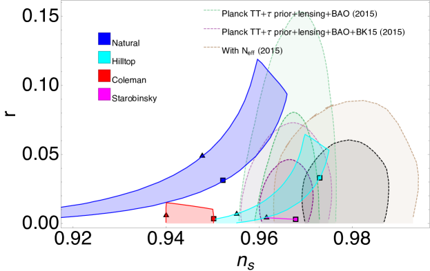
Figure 1: $n_{s}-r$ predictions for four inflationary models (Starobinsky Inflation, Natural Inflation, Hilltop Inflation, and Coleman-Weinberg Inflation) for $50\lesssim N_{\rm CMB}\lesssim 60$. The curves with a triangle on them correspond to $N_{\rm CMB}=50$, while the curves with a square on them correspond to $N_{\rm CMB}=60$. The green-shaded regions indicate the bound on $(n_{s},r)$ plane at $68\%$ and $95\%$ CL from the Planck2015 Planck:2015fie , and the purple-colored regions show bounds from the combined analysis of Planck2015+Bicep2-Keck Array2015 BICEP2:2018kqh for a standard value of $\Delta N_{\mathrm{eff}}$ ($\Delta N_{\mathrm{eff}}=0$). The regions with brown shading show the shifting of the same bounds when $\Delta N_{\mathrm{eff}}$ is varied (using Planck2015+Bicep2-Keck Array2015+baryon acoustic oscillation data + direct measured value of present-day Hubble constant, with $\Lambda$CDM+$r+N_{\mathrm{eff}}$ as parameters lead $\Delta N_{\mathrm{eff}}=0.254$) Guo:2017qjt ; Kannike:2018zwn . Predictions from Hilltop and Starobinsky inflation are within $1-\sigma$ CL from Planck2015+Bicep2-Keck Array2015 bound. However, when $\Delta N_{\mathrm{eff}}$ is used as a free parameter, S-I survives at $2-\sigma$ bound for higher number of ${\cal N}_{\text{CMB}}$ while H-I can satisfy $(n_{s},r)$ values within $1-\sigma$ bound.

III.1 Starobinsky Inflation ${\cal R}^{2}$ (S-I)

Starobinsky Inflationary (abbreviated as S-I) model is one of the simplest examples of plateau potentials with only one parameter, where no fine-tuning is needed for the inception of inflation. This is the inflationary model which depicts inflation by adding a term proportional to the square of Ricci curvature as a modification to Einstein-gravity. The action of S-I in Jordan frame is given by Starobinsky:1980te ; Mazumdar:2019tbm

$${\cal S}=\frac{M_{P}^{2}}{2}\int\text{d}^{4}x\sqrt{-g^{JF}}\left({\cal R}^{JF}+\frac{{{\cal R}^{JF}}^{2}}{6m_{SI}^{2}}\right)\,.$$ (11)

Here, superscript $JF$ implies that the corresponding parameter is defined in Jordan frame and $m_{SI}$ is the mass scale. This action can be converted to Einstein frame by a conformal transformation of the metric DeFelice:2010aj $g_{\mu\nu}=\Omega^{2}g^{JF}_{\mu\nu}$ where $\Omega^{2}=\ln\left(1+\frac{{\cal R}^{JF}}{3m_{SI}^{2}}\right)$. And then the action in $g_{\mu\nu}$ metric space takes a form similar to Eq. (4). Then the potential takes the form

$$V(\phi)=\Lambda^{4}\left(1-e^{-\sqrt{\frac{2}{3}}\frac{\phi}{M_{P}}}\right)^{2},$$ (12)

where the inflaton $\phi$ and $\Lambda^{4}$ are defined as Aldabergenov:2018qhs ; Martin:2013tda

$$\phi=\sqrt{\frac{3}{2}}M_{P}\ln\left(1+\frac{{\cal R}^{JF}}{3m_{SI}^{2}}\right)\,,\quad \Lambda^{4}=\frac{3}{4}M_{P}^{2}\,m_{SI}^{2}\,.$$ (13)

To satisfy CMB data of scalar fluctuations, $m_{SI}/M_{P}\sim{\cal O}(10^{-5})$. Now, the scalar spectral index and tensor-to-scalar ratio for the potential of Eq. (12) are

$$n_{s}=\frac{3\,e^{2\sqrt{\frac{2}{3}}\frac{\phi}{M_{P}}}-14\,e^{\sqrt{\frac{2}{3}}\frac{\phi}{M_{P}}}-5}{3\left(e^{\sqrt{\frac{2}{3}}\frac{\phi}{M_{P}}}-1\right)^{2}}\,,\quad\quad r=\frac{64}{3\left(e^{\sqrt{\frac{2}{3}}\frac{\phi}{M_{P}}}-1\right)^{2}}\,.$$ (14)

The slow-roll inflationary epoch ends when $\epsilon_{V}\sim 1$ happens. Furthermore, this S-I model predicts a very small value of $r$, and thus it is within $1-\sigma$ contour of the Planck2015+Bicep2 CMB bound (see the magenta colored region (line) in Fig. 1 for $50\leq N_{\rm CMB}\leq 60$. Since $n_{s}$ and $r$ do not depend on any parameter, this model cannot be further adjusted for the $n_{s}-r$ contour when $\Delta N_{\mathrm{eff}}$ is treated as a variable.

III.2 Natural Inflation (N-I)

For slow-rolling of the inflaton, the flatness of the potential needs to be maintained against radiative correction arising from self-interaction of the inflaton or its interaction with other fields. When the axion or the axionic field plays the role of inflaton, it provides the requisite mechanisms to protect the flatness of the potential. It also offers a proper explanation from particle physics, for the small values of the self-coupling and, thus, dilutes the issue of fine-tuning. That’s why this inflationary model is called Natural Inflation (abbreviated as N-I). Axion is a pseudo-Nambu-Goldstone boson that arises as a result of the spontaneous breaking of global symmetry followed by additional explicit symmetry breaking Freese:1990rb . The axion potential which arises due to the spontaneous breaking of global shift symmetry or axionic symmetry is given by Freese:1990rb

$$V(\phi)=\Lambda_{N}^{4}\left[1+\cos\left(\frac{\phi}{f_{a}}\right)\right]\,,$$ (15)

where $\Lambda_{N}$ is the $U(1)$ explicit symmetry-breaking energy scale, which determines the inflation scale, $f_{a}$ is the axion decay constant, and $\phi$ is the canonically normalized axion field. The first spontaneous $U(1)$ symmetry breaking happens when $T\simeq f_{a}$ ($T$ represents the temperature of the universe). $f_{a}$ also reduces the value of the self-coupling of the $\phi$ by $1/f_{a}$ Freese:1990rb . On the other hand, the axionic symmetry protects the flatness of the potential of axionic-inflaton Kim:2004rp , at least up to tree level Freese:1990rb .

The potential of Eq. (15) has a number of discrete maxima at $\phi=n\pi f_{a}$, with $n=1,3,\cdots$. At the vicinity of the location of the maximum of the potential, $\left|\eta_{V}\right|\approx 1/2f_{a}^{2}\ll 1$, and this sets the limit of $f_{a}$ Kim:2004rp . This inflationary model, like S-I, comes to an end when $\epsilon_{V}\sim 1$. $n_{s}$ and $r$ can now be calculated as

$$n_{s}=\frac{f_{a}^{2}-2\,M_{P}^{2}\,\sec^{2}\left(\frac{\phi}{2f_{a}}\right)+M_{P}^{2}}{f_{a}^{2}}\,,\qquad\qquad r=\frac{8\,M_{P}^{2}\,\tan^{2}\left(\frac{\phi}{2f_{a}}\right)}{f_{a}^{2}}\,.$$ (16)

The values of $n_{s}$ and $r$ for $10M_{P}\lesssim f_{a}\lesssim 1585M_{P}$ are shown in Fig. 1 as blue colored region. This inflationary model has been ruled out at $1-\sigma$ CL by Planck2015+Bicep2.

III.3 Hilltop Inflation (H-I)

In this inflationary model (abbreviated as H-I) inflaton starts rolling near the maximum of the potential and this automatically makes $\epsilon_{V}\sim 0$ at the onset of inflation. The potential is given by Kohri:2007gq ; Boubekeur:2005zm

$$V(\phi)=\Lambda_{H}^{4}\left[1-\left(\phi\over v\right)^{4}+...\right]\,,$$ (17)

where $\Lambda_{H}$ and $v$ are parameters, and the ellipsis represents the other higher-order terms that make the potential bounded from below, and may be responsible for creating the minimum. The maximum of the potential of Eq. (17) is at $\phi=0$. This inflationary model also ends with $\epsilon_{V}\sim 1$. $n_{s}$ and $r$ are given by

$$n_{s}=1-\frac{24\,M_{P}^{2}\,\phi^{2}\,\left(v^{4}+\phi^{4}\right)}{\left(v^{4}-\phi^{4}\right)^{2}}\,,\qquad r=\frac{128\,M_{P}^{2}\,\phi^{6}}{\left(v^{4}-\phi^{4}\right)^{2}}\,.$$ (18)

The values of $n_{s}$ and $r$ for $0.01M_{P}\lesssim v\lesssim 100M_{P}$ exist well inside the $2-\sigma$ range and are shown as cyan-colored region in Fig. 1.

III.4 Coleman-Weinberg Inflation (C-I)

This potential of Coleman-Weinberg Inflation (abbreviated as C-I) is actually the effective potential of quartic self-interacting scalar field up to 1-loop order, and it is given by Barenboim:2013wra ; Okada:2014lxa ; Kallosh:2019jnl ; Choudhury:2011sq

$$V(\phi)=\frac{Af^{4}}{4}+A\phi^{4}\left[\log\left(\frac{\phi}{f}\right)-\frac{1}{4}\right].$$ (19)

Here $f=\left<\phi\right>$ is the renormalization scale and $V(\phi=f)=V^{\prime}(\phi=f)=0$. $A=A(f)$ is determined by the beta function of the scalar-quartic-coupling with inflaton. Here, we do not go into detailed models of interaction of $\phi$ with other fields, and we take $A$ as a free parameter, and fixed it by the normalization to the amplitude of the CMB anisotropies. The model predicts $n_{s}$ and $r$ as

$$n_{s} = 1+\frac{32\,M_{P}^{2}\,\phi^{2}\left[\left(3f^{4}+12\,\phi^{4}\,\log\left(\frac{f}{\phi}\right)+\phi^{4}\right)\log\left(\frac{\phi}{f}\right)+f^{4}-\phi^{4}\right]}{\left(f^{4}+4\phi^{4}\log\left(\frac{\phi}{f}\right)-\phi^{4}\right)^{2}}\,,$$ (20)

$$r = \frac{2048\,M_{P}^{2}\,\phi^{6}\,\log^{2}\left(\frac{\phi}{f}\right)}{\left(f^{4}+4\,\phi^{4}\,\log\left(\frac{\phi}{f}\right)-\phi^{4}\right)^{2}}\,.$$ (21)

In comparison to previous inflationary models, here we are assuming small-filed inflationary scenario with $\phi^{*}\ll f,\phi_{\rm end}\ll f$ and it ends with $\left|\eta_{V}\right|\sim 1$. $n_{s}-r$ predictions for C-I for different values of $f$ are shown in Fig. 1 as red-colored region. This model is already ruled even out at $2-\sigma$ level by Planck2015 data.

Along with the Planck2015 and Planck2015+Bicep2-Keck Array2015 combined bounds and theoretical predictions for $n_{s}-r$ for the four above-mentioned inflationary models, Fig. 1 also displays $n_{s}-r$ contour (brown-colored region on $(n_{s},r)$ plane) from Ref. Guo:2017qjt at $1-\sigma$ and $2-\sigma$ CL where $\Delta N_{\mathrm{eff}}$ is regarded as an independent variable. To draw this contour, the dataset used are Planck2015 + Bicep2 + Keck Array B-mode CMB data + baryon acoustic oscillation (BAO) data + direct measured present-day-value of Hubble parameter ${\cal H}_{0}$ with $\Lambda$CDM$+r+N_{\mathrm{eff}}$ model. They found the best-fit parameter value $\Delta N_{\mathrm{eff}}=0.254$ and $n_{s}=0.9787$. Fig. 1 also exhibits that H-I can satisfy the $(n_{s},r)$ values, even in $1-\sigma$ range for ${\cal N}_{\text{CMB}}\sim 60$. Predictions from S-I, on the contrary, can fit in $2-\sigma$ region for larger values of ${\cal N}_{\text{CMB}}$ while remaining outside of $2-\sigma$ boundary for ${\cal N}_{\text{CMB}}\sim 50$.

IV Inflaton decay during reheating

Our discussion in the preceding section is independent of the origin of $\Delta N_{\mathrm{eff}}$. In this section, we assume that a BSM particle which contributes to $\Delta N_{\mathrm{eff}}$, is produced from the inflaton during the reheating epoch. As soon as the slow-roll phase ends, the equation of state parameter becomes $w>-(1/3)$, and inflaton quickly descends to the minimum of the potential and initiates damped coherent oscillations of inflaton about this minimum and the reheating era begins. The energy density of this oscillating field is assumed to behave as a non-relativistic fluid with no pressure when averaged over a number of coherent oscillations. Therefore, the averaged equation of state parameter during reheating $\bar{w}_{r}=0$. During this epoch, the energy density of this oscillating inflaton reduces due to Hubble expansion. In addition to that, the energy density of inflaton also decreases owing to interaction with the relativistic SM Higgs and possibly with a relativistic BSM particle, $X$, which eventually contributes to the effective number of neutrinos Ichikawa:2007jv . During the initial phase of this epoch, ${\cal H}>\Gamma_{\phi}$. Here, $\Gamma_{\phi}$ is the effective dissipation rate of inflaton, and the small value of $\Gamma_{\phi}$ is due to the small value of the couplings with inflaton. However, the value of ${\cal H}$ continues to decrease, and soon it becomes ${\cal H}\sim\Gamma_{\phi}$. Approximately at this time, the energy density of oscillating inflaton and the energy density of relativistic species produced from the decay of inflaton become equal. At this moment, the temperature of the universe, $T_{\rm RH}$, is given by Lozanov:2019jxc ; Giudice:2000ex ; Garcia:2020wiy

$$T_{\rm RH}=\left(\frac{90}{g_{\star{,\rm RH}}\,\pi^{2}}\right)^{1/4}\sqrt{\Gamma_{\phi}\,M_{P}}\,,$$ (22)

where $g_{\star{,\rm RH}}$ denotes the effective number of degrees of freedom at the conclusion of the reheating era. We also assume that inflaton decays instantly and completely during the last stage of the reheating era, and the universe thereafter becomes radiation dominated. If ${a}_{\rm RH}$ is the cosmological scale factor at the end of reheating, then, the number of $e$-folds during reheating, ${\cal N}_{\rm RH}$, is given by Drewes:2017fmn

$${\cal N}_{\rm RH}\equiv\log\left(\frac{{a}_{\rm RH}}{{a}_{\rm end}}\right)=\frac{1}{3}\ln\left(\frac{\rho_{\rm end}}{3\,\Gamma_{\phi}^{2}\,M_{P}^{2}}\right)\,,$$ (23)

where $\rho_{\rm end}$ is the energy density at the end of inflation. To derive this, we have used Eq. (22), and the fact that the universe becomes radiation dominated at the end of reheating, and also assumed that equation of state does not vary during reheating epoch. If slow roll inflation ends with $\epsilon_{V}(\phi_{\rm end})=1$ (i.e. with $\dot{\phi}^{2}|_{\phi=\phi_{\rm end}}=V(\phi_{\rm end})$), then

$$\rho_{\rm end}=\left(1+\frac{\epsilon_{V}(\phi_{\rm end})}{3}\right)\,V(\phi_{\rm end})=\frac{4}{3}V(\phi_{\rm end})\,.$$ (24)

Again, rearranging Eq. (23), we get

$$\Gamma_{\phi}=\frac{1}{M_{P}}\left(\frac{\rho_{\rm end}}{3}\right)^{1/2}e^{-3\,{\cal N}_{\rm RH}/2}\,.$$ (25)

Now, if $\Gamma_{\phi\to XX}$ and $\Gamma_{\phi\to hh}$ are the decay width of inflaton to $X$ and SM Higgs particle $h$, then the branching fraction $B_{X}$ for the production of $X$ particle is defined as

$$B_{X}=\frac{\Gamma_{\phi\to XX}}{\Gamma_{\phi\to XX}+\Gamma_{\phi\to hh}}=\frac{\Gamma_{\phi\to XX}}{\Gamma_{\phi}}\,.$$ (26)

Here, $\Gamma_{\phi}=\Gamma_{\phi\to XX}+\Gamma_{\phi\to hh}$. Now, the time evolution of the energy density of inflaton, $\rho_{\phi}$, energy density of relativistic SM particles, $\rho_{\rm rad}$, and energy density of relativistic $X$ particle, $\rho_{X}$, can be computed by solving the following set of differential equations

$$\dot{\rho}_{\phi}+3\,{\cal H}\,\rho_{\phi}=-\Gamma_{\phi}\,\rho_{\phi}\,,$$ (27)

$$\dot{\rho}_{\rm rad}+4\,{\cal H}\,\rho_{\rm rad}=\Gamma_{\phi}\,(1-B_{X})\,\rho_{\phi}\,,$$ (28)

$$\dot{\rho}_{X}+4\,{\cal H}\,\rho_{X}=\Gamma_{\phi}\,B_{X}\,\rho_{\phi}\,.$$ (29)

Here, we assume that $X$ is so feebly interacting with $H$ or other SM particles that we can ignore the interaction term. Besides, we also assume that $X$-particles are not self-interacting. Therefore, $\rho_{X}$ only decreases due to Hubble-expansion of the universe. Furthermore, the Friedmann equation gives

$${\cal H}^{2}=\frac{\rho_{\phi}+\rho_{\rm rad}+\rho_{X}}{3M_{P}^{2}}\,.$$ (30)

This $X$ particle fails to establish thermal equilibrium with the thermal SM relativistic fluid of the universe, and hence does not share the temperature of photons or neutrinos. This BSM article remains relativistic up to today, and thus contributes to the total relativistic energy density of the present universe

$$\rho_{{\rm rad},{\rm tot}} =\rho_{\gamma}+\rho_{\nu}+\rho_{X}\,.$$ (31)

Following Sec. II, we claim that $N_{\mathrm{eff}}$ takes care of the contribution of $X$ to $\rho_{{\rm rad},{\rm tot}}$, and in the absence of $X$ particle, $N_{\mathrm{eff}}={N_{\mathrm{eff}}}_{,\text{SM}}$. The contribution of $X$ in $N_{\mathrm{eff}}$ is expressed as Jinno:2012xb

$$\Delta N_{\mathrm{eff}}=\frac{43}{7}\quantity[\frac{10.75}{g_{\star,s{,\rm RH}}}]^{1/3}\quantity[\frac{\rho_{X}}{\rho_{\rm rad}}]_{{\cal H}\ll\Gamma_{\phi}}\,.$$ (32)

The subscript ${\cal H}\ll\Gamma_{\phi}$ implies that the integration has been done till the reheating process is over. In Eq. (32), $g_{\star,s{,\rm RH}}$ is the effective degrees of freedom contributing to the entropy density of the universe at the time when $\rho_{\phi}$ decays completely. We are assuming that $g_{\star,s{,\rm RH}}\approx 106.75$, and it remains the same throughout the reheating process.

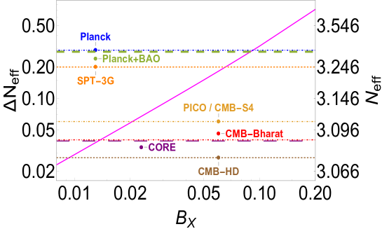
Figure 2: $\Delta N_{\mathrm{eff}}$ against $B_{X}$ following Eq. (32). The parallel horizontal lines indicate present bounds on $\Delta N_{\mathrm{eff}}$ and prospective future reaches that will be within the scope of the sensitivity of the upcoming CMB observations mentioned in Table. 1. If the non-thermal $X$-particle is created only from inflaton decay, then it should be $B_{X}\lesssim 0.09$ (Planck bound). If $B_{X}\gtrsim 0.009$, then it can be tested further by future CMB observations.

Now, using the bounds on $\Delta N_{\mathrm{eff}}$ and prospective future reaches of $\Delta N_{\mathrm{eff}}$ from Table 1, $\Delta N_{\mathrm{eff}}$ as a function of $B_{X}$ from Eq. (32) (and assuming that $B_{X}$ does not depend on cosmological scale factor) is shown in Fig. 2. Because a higher value of $B_{X}$ suggests a higher production of $X$ particles, $\Delta N_{\mathrm{eff}}$ grows monotonically with $B_{X}$. This is true when $\Delta N_{\mathrm{eff}}$ is solely contributed by $X$ particle. On the other hand, the terms on the right-hand-side of Eqs. (28) and (29) are the production rate of radiation and $X$, respectively, and only $B_{X}$ regulates the difference between those two production rates. Since $\Delta N_{\mathrm{eff}}\sim\rho_{X}/\rho_{\rm rad}$, the result shown in Fig. 2 is independent of whether $\Gamma_{\phi}$ is constant or varies with cosmological scale factor and temperature (e.g. Barman:2022tzk ). Additionally, this figure depicts that Planck and Planck+BAO bounds draw an upper limit on the possible values of $B_{X}$. $B_{X}>0.09$ is already eliminated by Planck data. Furthermore, $0.09\gtrsim B_{X}\gtrsim 0.066$ can be tested by spt-3g, and $B_{X}\gtrsim 0.021,B_{X}\gtrsim 0.014,B_{X}\gtrsim 0.013,$ and $B_{X}\gtrsim 0.009$ may be tested from other future CMB experiments such as CMB-S4/PICO, CMB-Bh$\overline{a}$rat, CORE, and CMB-HD.

We use the relation between $\Delta N_{\mathrm{eff}}$ and $B_{X}$ from Fig. 2 in Fig. 3 where allowed ranges of $r$ for the four inflationary models are shown as colored horizontal-stripes on $(r,B_{X}/\Delta N_{\mathrm{eff}})$ plane. On the left panel, the green and yellow colored region exhibits allowed range for $r$ for N-I and H-I models. The cyan and brown colored region on the right panel of Fig. 3 illustrates the allowed range for $r$ for the other two inflationary models – C-I and S-I, respectively. The $68\%$ and $95\%$ CL contours depicted on the background on this $(r,B_{X}/\Delta N_{\mathrm{eff}})$ plane are taken from DiValentino:2016ucb,Refs. Ref. DiValentino:2016ucb . These 2-dimensional contours are from $8$-parameter analysis, including $r$ and $N_{\mathrm{eff}}$, of Planck and Bicep data, assuming $\Lambda$CDM and flat universe. The datasets used here are the combined Planck2015 temperature power spectrum ($2<\ell<2500$, $\ell$ is the multipole number, and indicates an angular scale on the sky of roughly $\pi/\ell$ Bambi:2015mba ) with polarization power spectra for $(2<\ell<29)$ (“PlanckTT + lowTEB”) Planck:2015bpv , high multipoles Planck polarization data with CMB polarization B modes constraints provided by the 2014 common analysis of Planck2015, Bicep2 and Keck Array (“PlanckTTTEEE + lowTEB+BKP”) BICEP2:2015nss , and 2016 dataset from Planck High Frequency Instrument (HFI) (”tau”) Planck:2016kqe . The best fit value of $\Delta N_{\mathrm{eff}}$ at $68\%$ CL are $0.504$ for “PlanckTT + lowTEB”, $0.094$ for “TTTEEE+tau”, $0.464$ for “PlanckTTTEEE + lowTEB+BKP”. Regarding PlanckTT + lowTEB dataset, all of these four inflationary models are ruled out at more than $2-\sigma$. Fig. 3 also shows that four inflationary models will be within $2-\sigma$ contour of ‘TTTEEE+tau’ data if $B_{X}\gtrsim 0.033$ (for N-I), $B_{X}\gtrsim 0.061$ (for H-I), $B_{X}\gtrsim 0.097$ (for C-I), $B_{X}\gtrsim 0.11$ (for S-I). Similarly, to be within $2-\sigma$ contour of ‘TTTEEE+lowTEB+BKP’ it is required that $B_{X}\gtrsim 0.046$ (for N-I), $B_{X}\gtrsim 0.07$ (for H-I), $B_{X}\gtrsim 0.13$ (for C-I), $B_{X}\gtrsim 0.15$ (for S-I). By using this now along with the Fig. 2, it is possible to determine whether any inflationary model is compatible with the assumption that inflaton is the only source of $X$ and this $X$ contributes solely and entirely to $N_{\mathrm{eff}}$. For instance, S-I and C-I inflation are incompatible with the aforementioned assumption regarding the ‘TTTEEE+tau’ and ‘TTTEEE+lowTEB+BKP’ dataset. If $X$ originates from a different source, these inflationary models can still remain inside $1-\sigma$ contour of ‘TTTEEE+tau’ data. In contrary, H-I is compatible with the assumption that inflaton is the sole source of $X$, at least, up to $2-\sigma$ CL interval. It is also worth noting that, the best fit value of $n_{s}$ varies in presence of $N_{\mathrm{eff}}$, just like the best-fit value of $r$. As a result, Fig. 3 cannot be utilized to make the final decision to validate any inflationary models. In Fig. 3, the N-I model, for example, predicts r value within $2-\sigma$ bounds, but this model is already ruled out in Fig. 1 due to the predicted small value of $n_{s}$.

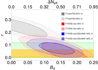
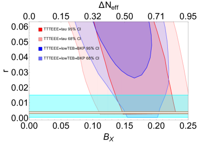
Figure 3: Left panel: Constraints on $(r,B_{X})$ plane at $68\%$ and $95\%$ CL from Ref. DiValentino:2016ucb combining Planck 2015 temperature power spectrum (“PlanckTT + lowTEB”), high multipoles Planck polarization data with CMB polarization B modes constraints provided by the 2014 common analysis of Planck, Bicep2 and Keck Array (“PlanckTTTEEE + lowTEB+BKP”), and 2016 dataset from Planck High Frequency Instrument (HFI) (”tau”). The region covered with light green color indicates the allowed region of $r$ predicted by N-I model, while the yellow-shaded region corresponds to the prediction from H-I inflationary model. Right panel: same bound on $(r,B_{X})$ plane as the left panel, but with predictions of $r$ from C-I (cyan-colored region) and from S-I (brown-colored region). All of these models have been ruled out by ‘PlanckTT + lowTEB’ data on $(r,B_{X}/\Delta N_{\mathrm{eff}})$ plane. Although, N-I and H-I remains within $1-\sigma$ limit of both ‘TTTEEE+tau’ and ‘PlanckTTTEEE + lowTEB+BKP’ data, C-I and S-I are within $1-\sigma$ contour of only ‘PlanckTTTEEE + lowTEB+BKP’ data.

V Inflaton Decaying to Dark Radiation

Following the preceding section, we postulate that during reheating, the inflaton decays to SM Higgs doublet $H$ and BSM particle $X$. The Lagrangian density describing such a process can be expressed as Drewes:2017fmn ; Drewes:2019rxn ; Lozanov:2019jxc ; Allahverdi:2010xz

$${\cal L}\supset-\lambda_{12,H}\,\sigma_{m}\,\phi\,H^{\dagger}H-{\cal L}_{\phi\to X}\,-{\cal L}_{\rm scattering}\,,$$ (33)

where the first term on the right side of Eq. (33) encodes the decay of $\phi$ to the SM Higgs particle $h$, and hence this term is accountable for the generation of thermal relativistic SM plasma of the universe. $\lambda_{12,H}$ is dimensionless in this case, and $\sigma_{m}$, the mass scale, is taken to be equal to $m_{\phi}$. Subsequently, the decay width to SM Higgs particle $h$ is

$$\Gamma_{\phi\to{hh}}\simeq\frac{\lambda_{12,H}^{2}\,\sigma_{m}^{2}}{8\pi\,m_{\phi}}=\frac{\lambda_{12,H}^{2}\,m_{\phi}}{8\pi\,}\,,$$ (34)

In Secs. III.1, III.2, III.3 and III.4, we have discussed four inflationary scenarios. The minimum of the potential of N-I is located at $f\pi$, whereas for S-I, it is at $\phi=0$, and for C-I, it is at $\phi=f$. Then, the masses of inflaton for the aforementioned three inflationary models are

$$m_{\phi}=\begin{cases}\frac{2}{\sqrt{3}}\frac{\Lambda^{2}}{M_{P}}\qquad&\text{(for S-I~{}\cite[cite]{\@@bibref{Authors Phrase1YearPhrase2}{DiValentino:2016nni}{\@@citephrase{(}}{\@@citephrase{)}}})}\,,\\ \frac{\Lambda_{N}^{2}}{f_{a}}\,\qquad&\text{(for N-I~{}\cite[cite]{\@@bibref{Authors Phrase1YearPhrase2}{Freese:2014nla}{\@@citephrase{(}}{\@@citephrase{)}}})}\,,\\ 2\sqrt{A}f\qquad&\text{(for C-I~{}\cite[cite]{\@@bibref{Authors Phrase1YearPhrase2}{Panotopoulos:2021ttt}{\@@citephrase{(}}{\@@citephrase{)}}})}\,.\end{cases}$$ (35)

Since, $\Lambda,\Lambda_{N},f_{a},A$, and $f$ are determined from the best-fit value of $n_{s},r,A_{s}$ obtained from CMB data and the number of $e$-folds ${\cal N}_{\rm CMB}$, $m_{\phi}$ for the aforementioned three inflationary models are determined by the data from CMB observations. However, it should be noted that N-I and C-I are already in discordance with $n_{s}-r$ contour from BICEP data, even at $2-\sigma$ CL (see Figs. 1 and 7). Furthermore, the form of the potential of Hilltop model, as described in Eq. 17, is expected to be bounded from below by other terms without affecting the inflationary predictions. Therefore, it becomes necessary to consider a specific theory to define the mass of the inflaton in this scenario (See Ref. Kallosh:2019jnl , for further details).

To keep the discussion of this section more general, we consider a broader range of inflationary scenarios beyond the four inflationary scenarios discussed above. For example, if we consider quartic inflationary potential, we need to add a bare mass term to study reheating (for example, see. Dimopoulos:2017xox,Refs. Ref. Dimopoulos:2017xox ). This is why, instead of fixing a specific value, we explore variations in the $m_{\phi}$ during our analysis.

Furthermore, ${\cal L}_{\phi\to X}$ in Eq. (33) is the interaction term of $\phi$ with $X$. Let us also assume that $\lambda_{\phi X}$ is the coupling of inflaton-BSM particle interaction. Now, to make the discussion as generic as feasible, we suppose that $X$ can be a light fermion $\chi$, a BSM scalar $\varphi$, or a $U(1)$ gauge boson $\upgamma$. Therefore, possible interaction Lagrangian with $\phi$ includes Drewes:2019rxn ; Drewes:2017fmn

$$+y_{\chi}\,\phi\,\bar{\chi}\chi\,, \left(\phi\to\bar{\chi}\chi\,;\quad\lambda_{\phi X}\equiv y_{\chi}\right)\,,$$ (36)

$$+\lambda_{12,\varphi}\,\sigma^{\prime}_{m}\,\phi\,\varphi\varphi\,, \left(\phi\to\varphi\varphi\,;\quad\lambda_{\phi X}\equiv\lambda_{12,\varphi}\right)\,,$$ (37)

$$+\frac{\lambda_{13,\varphi}}{3!}\,\phi\,\varphi\varphi\varphi\,, \left(\phi\to\varphi\varphi\varphi\,;\quad\lambda_{\phi X}\equiv\lambda_{13,\varphi}\right)\,,$$ (38)

$$+\frac{g_{\phi\upgamma}}{\Lambda_{m}}\,\phi\,F_{\mu\nu}\tilde{F}^{\mu\nu}\,, \left(\phi\to\upgamma\upgamma\,;\quad\lambda_{\phi X}\equiv g_{\phi\upgamma}\right)\,.$$ (39)

Here $y_{\chi},\,\lambda_{12,\varphi},\,\lambda_{13,\varphi},$ and $g_{\phi\upgamma}$ are dimensionless couplings with $\sigma^{\prime}_{m},\Lambda_{m}$ as mass scales. $F_{\mu\nu}$ is the field strength tensor of $\upgamma$, and $\tilde{F}^{\mu\nu}$ is its dual. Additionally, ${\cal L}_{\rm scattering}$ in Eq. 33 represents the scattering terms involving inflaton with both SM and BSM particles, and can be written as follows

$${\cal L}_{\rm scattering} =\lambda_{22}\,\phi\phi\,H^{\dagger}H+{\cal L}_{\phi\phi\to XX}+\text{h.c.}\,,$$ (40)

where $\lambda_{22}$ is dimensionless couplings. We assume that ${\cal L}_{\phi\phi\to XX}$-channel is not effective in contribution to $N_{\mathrm{eff}}$. For instance, for $\phi\phi\to\varphi\varphi$ channel, we can write Drewes:2019rxn

$${\cal L}_{\phi\phi\to XX}=+\frac{\lambda_{22,\varphi}}{4}\,\phi\phi\,\varphi\varphi\,,\qquad \left(\phi\phi\to\varphi\varphi\,;\quad\lambda_{\phi X}\equiv\lambda_{22,\varphi}\right)\,.$$ (41)

In Appendix C, we show that the contribution of $\varphi$ producing via Eq. 41 in $\Delta N_{\mathrm{eff}}$ is negligible compared to $\varphi$ produced via $\phi\to\varphi\varphi$ decay channel, due to the reaction rate in the former case being dependent on the instantaneous value of inflaton energy density. In Appendix D, we explore the range of these couplings to investigate whether DR can achieve thermal equilibrium with SM Higgs via inflaton exchange processes.

Now, the reaction rates for the interactions from Eqs. 37, 36 and 39, in leading order, and related branching fractions are as follows:

$$\Gamma_{\phi\to\chi\chi}\simeq\frac{y_{\chi}^{2}\,m_{\phi}}{8\pi}\,, B_{\chi}=\frac{\left(y_{\chi}/\lambda_{12,H}\right)^{2}}{1+\left(y_{\chi}/\lambda_{12,H}\right)^{2}}\, \left(\text{If}\,X\equiv\chi,\,\text{and}\,\phi\to\bar{\chi}\chi\right),$$ (42)

$$\Gamma_{\phi\to\varphi\varphi}\simeq\frac{\lambda_{12,\varphi}^{2}\,{\sigma^{\prime}_{m}}^{2}}{8\pi\,m_{\phi}}\,, B_{\varphi}=\frac{\left(\lambda_{12,\varphi}/\lambda_{12,H}\right)^{2}}{\left(m_{\phi}/{\sigma^{\prime}_{m}}\right)^{2}+\left(\lambda_{12,\varphi}/\lambda_{12,H}\right)^{2}}\, \left(\text{If}\,X\equiv\varphi,\,\text{and}\,\phi\to\varphi\varphi\right),$$ (43)

$$\Gamma_{\phi\to\varphi\varphi\varphi}=\frac{\lambda_{13,\varphi}^{2}\,m_{\phi}}{3!64(2\pi)^{3}}\,, B_{\varphi}=\frac{\left(\lambda_{13,\varphi}/\lambda_{12,H}\right)^{2}}{384\pi^{2}+\left(\lambda_{13,\varphi}/\lambda_{12,H}\right)^{2}}\, \left(\text{If}\,X\equiv\varphi,\,\text{and}\,\phi\to\varphi\varphi\varphi\right),$$ (44)

$$\Gamma_{\phi\to\upgamma\upgamma}=\frac{g_{\phi\upgamma}^{2}}{4\pi\,\Lambda_{m}^{2}}\,m_{\phi}^{3}\,, B_{\upgamma}=\frac{\left(g_{\phi\upgamma}/\lambda_{12,H}\right)^{2}}{(1/2)\left(\Lambda_{m}/m_{\phi}\right)^{2}\,+\left(g_{\phi\upgamma}/\lambda_{12,H}\right)^{2}}\, \left(\text{If}\,X\equiv\upgamma,\,\text{and}\,\phi\to\upgamma\upgamma\right).$$ (45)

In this work, we assume $\sigma^{\prime}_{m}=\epsilon_{1}\,m_{\phi}$ and $\Lambda_{m}=\epsilon_{2}\,m_{\phi}$ where $\epsilon_{1},\epsilon_{2}$ are dimensionless and $\subset\mathbb{R}_{>0}$. Consequently, $B_{\chi}$, $B_{\varphi}$ (from Eqs. (43) and (44)), and $B_{\upgamma}$ are independent of $m_{\phi}$. Then, in Fig. 4, we explore the allowable area on the 2-dimensional parameter-space of $(\lambda_{\phi X},\lambda_{12,H})$ for the interactions from Eqs. (36)-(39), regarding the present bounds on $\Delta N_{\mathrm{eff}}$ and prospective future reaches of $\Delta N_{\mathrm{eff}}$ that will be within the scope of future exploration by upcoming CMB observations listed in Table 1. Here, we set all the mass scales to $\sigma^{\prime}_{m}=\Lambda_{m}=m_{\phi}$. Furthermore, in order to prevent nonperturbative particle production from becoming significant during reheating, we maintain the values of the couplings below ${\cal O}(10^{-4})$ Ghoshal:2022fud ; Drewes:2019rxn . We observe that for a given value of $\Delta N_{\mathrm{eff}}$, a greater value of $\lambda_{12,H}$ implies a higher value of the coupling of the inflaton with the BSM particle. This is to be expected because a higher value of $\lambda_{12,H}$ implies more generation of SM relativistic particles. To maintain $N_{\mathrm{eff}}$ constant, a greater value of the coupling of the dark sector to inflaton is required. The red solid line stands for $\Delta N_{\mathrm{eff}}=0.28$ implying that Planck+BAO rules out the region above this line. The dashed lines are prospective future reaches that will be within the range of exploration from upcoming CMB experiments with higher sensitivity. We do not present the region plot separately for $\phi\to\varphi\varphi$ since $B_{\varphi}$ for this process on $(\lambda_{12,\varphi},\lambda_{12,H})$ plane has similar form of $B_{\chi}$ on $(y_{\chi},\lambda_{12,H})$ plane. However, following the discussion of Appendix D, we should consider a lower range of $\lambda_{12,\varphi}$ to prevent the scalar DR particles from reaching thermal equilibrium with SM Higgs. To remain within Planck bound, $y_{\chi}/\lambda_{12,H}\lesssim 0.31$. Contrarily, for $\phi\to\varphi\varphi\varphi$, $\lambda_{13,\varphi}/\lambda_{12,H}\lesssim 19.37$ and for $\phi\to\upgamma\upgamma$, $g_{\phi\upgamma}/\lambda_{12,H}\lesssim 0.23$. The presence of $1/2$ and $384\pi^{2}$ in the denominator of the branching fraction in Eqs. (44) and (45) results in these differing upper bounds on the coupling ratios.

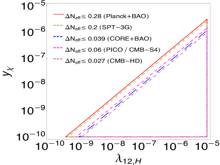
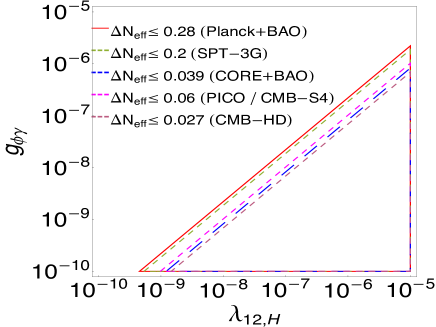
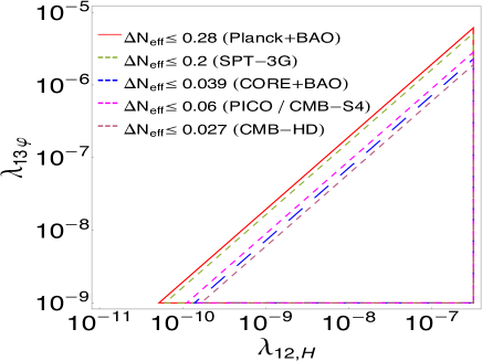
Figure 4: Colored lines delimit regions corresponding to the value of $\Delta N_{\mathrm{eff}}\leq$ current bounds and prospective future reaches that will be within the scope of upcoming CMB experiments, mentioned in Table. 1. The solid line is for Planck+BAO bound, and the region above this line is already ruled out. The dashed-lines are for prospective future reaches that will be within the scope of exploration from upcoming CMB observations and the parameter space above those dashed-lines could potentially be measured by upcoming CMB observations. Different colors have been used to represent different bounds from different CMB observations. Top-left panel displays such regions for $\phi\to\tilde{\chi}\chi$ on $(y_{\chi},\lambda_{12,H})$ plane. Similar regions can be obtained for $(\phi\to\varphi\varphi)$ on $(\lambda_{12,\varphi},\lambda_{12,H})$ plane for $\sigma^{\prime}_{m}=m_{\phi}$ (see the similarity between the branching fraction of Eq. (42) and Eq. (43)). Top-right panel and bottom panel illustrate such regions for $\phi\to\upgamma\upgamma$ on $(g_{\phi\upgamma},\lambda_{12,H})$ plane and for $\phi\to\varphi\varphi\varphi$ on $(\lambda_{13,\varphi},\lambda_{12,H})$ plane, respectively.

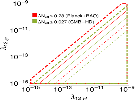
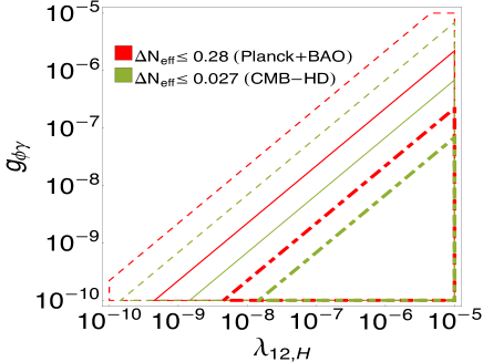
Figure 5: Illustration of the alteration of the permissible area on $(\lambda_{\phi X},\lambda_{12,H})$ plane when $\sigma^{\prime}_{m},\Lambda_{m}\neq m_{\phi}$. Solid lines represent $\sigma^{\prime}_{m}=\Lambda_{m}=m_{\phi}$ whereas dashed and dashed-dot lines indicate $\sigma^{\prime}_{m}=\Lambda_{m}=10\,m_{\phi}$ and $\sigma^{\prime}_{m}=\Lambda_{m}=0.1\,m_{\phi}$, respectively.   Left-panel is for $\phi\to\varphi\varphi$ and   right panel is for $\phi\to\upgamma\upgamma$. Red color lines are corresponded to $\Delta N_{\mathrm{eff}}=0.28$ (current bound from Planck+BAO) and green colored lines belong to $\Delta N_{\mathrm{eff}}=0.027$ (prospective future reach of $\Delta N_{\mathrm{eff}}$ of upcoming observation – CMB-HD). The area above the lines are excluded (within the future reach) by Planck (CMB-HD).

In Fig. 5, we consider current bound on $\Delta N_{\mathrm{eff}}$ - bounds from Planck and only one prospective future reach of $\Delta N_{\mathrm{eff}}$ that could be observed by CMB-HD, to demonstrate the shift in the allowable region on the respective $(\lambda_{\phi X},\lambda_{12,H})$ space for the choice of respective mass scales either greater or smaller than $m_{\phi}$ for $\phi\to\varphi\varphi$ and $\phi\to\upgamma\upgamma$. Similar to Fig. 4, here also the area above the lines are excluded or to be identified by present or future CMB observations. If we choose $\sigma^{\prime}_{m}>m_{\phi}$ and $\sigma^{\prime}_{m}<m_{\phi}$, the allowed area decreases and increases for $\phi\to\varphi\varphi$ and it is displayed on the left panel of Fig. 5. Contrarily, the right panel of this figure exhibits that increment or reduction of the permissible area for the choice of $\Lambda_{m}$ less or larger than $m_{\phi}$. This conclusion is in congruence with the expression of $B_{\varphi}$ and $B_{\upgamma}$ from Eqs. (43) and (45).

Lines with fixed values of the coupling of inflaton-BSM particle interaction (inclined lines) on $(\Delta N_{\mathrm{eff}},\lambda_{12,H})$ plane are shown in Fig. 6. This figure shows that for a certain value of $\lambda_{\phi X}$, $\Delta N_{\mathrm{eff}}$ grows as the value of $\lambda_{12,H}$ decreases. A lower value of $\lambda_{12,H}$ suggests less production of SM relativistic particle, and thus the ration in Eq. (32) increases. Fig. 6 also gives a comparative view how the range of $\lambda_{\phi X}$ varies for a given $\lambda_{12,H}$ $(10^{-5}\geq\lambda_{12,H}\geq 10^{-10})$ and for the same range of $\Delta N_{\mathrm{eff}}$ $(0.29>\Delta N_{\mathrm{eff}}\geq 0.027)$ for different possible interactions of $X$ with $\phi$. For example, the required ranges for $\lambda_{\phi X}$ for different interaction channels are - $10^{-11}\lesssim y_{\chi}\lesssim 10^{-6}$, $10^{-9}\lesssim\lambda_{13,\varphi}\lesssim 10^{-4}$. Additionally, this figure illustrates the allowed range of the value of the coupling $\lambda_{12,H}$ regarding the Planck bound on $\Delta N_{\mathrm{eff}}$ for a given value of $\lambda_{\phi X}$. Moreover, for a given value of $\lambda_{\phi X}$, this figure shows the value of $\lambda_{12,H}$ that are in compliance with Planck bound on $\Delta N_{\mathrm{eff}}$. For instance, the value $\lambda_{12,H}$ should be $<3.26\times 10^{-9}$ for $y_{\chi}=10^{-9}$. Furthermore, the dashed-magenta colored line correspond to $\Delta N_{\mathrm{eff}}=0.254$, the best fit value predicted by Ref. Guo:2017qjt . The point where this line intersects with the inclined lines in that figure, gives the values of the coupling-pairs $(\lambda_{12,H},\lambda_{\phi X})$ correspond to the bound on $(n_{s},r)$ plane when $N_{\mathrm{eff}}$ used as a free parameter in Fig. 1.

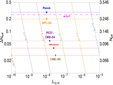
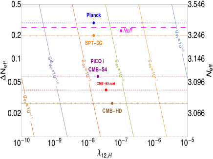
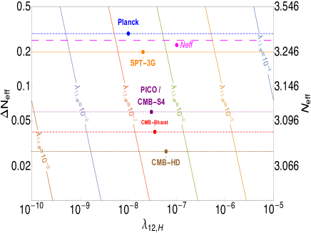
Figure 6: Inclined lines correspond to fixed values of the inflaton-BSM particle couplings on $(\Delta N_{\mathrm{eff}},\lambda_{12,H})$ plane. For this figure, we set all mass scales $\sim m_{\phi}$. The CMB experimental reaches on $\Delta N_{\mathrm{eff}}$ from Table 1 are shown by discontinuous-horizontal lines. The dashed line in magenta color indicates $\Delta N_{\mathrm{eff}}=0.254$, the value predicted by Ref. Guo:2017qjt .   Top-left panel,   top-right panel and   bottom panel are for $\phi\to\tilde{\chi}\chi$, $\phi\to\upgamma\upgamma$, and for $\phi\to\varphi\varphi\varphi$, respectively.

V.1 Reheat temperature

For the values of couplings shown in Fig. 6, the order of $T_{\rm RH}/\sqrt{M_{P}\,m_{\phi}}\sim 7.60\times 10^{-10}$ (for $\phi\to\tilde{\chi}\chi$ with $B_{\chi}\sim 0.02,\,y_{\chi}\sim 10^{-9},\,\lambda_{12,H}\sim 6.97\times 10^{-9}$), $T_{\rm RH}/\sqrt{M_{P}\,m_{\phi}}\sim 10.64\times 10^{-10}$ (for $\phi\to\upgamma\upgamma$ with $B_{\upgamma}\sim 0.021,\,g_{\varphi\upgamma}\sim 10^{-9},\,\lambda_{12,H}\sim 9.76\times 10^{-9}$), $T_{\rm RH}/\sqrt{M_{P}\,m_{\phi}}\sim 12.22\times 10^{-10}$ (for $\phi\to\varphi\varphi\varphi$ with $B_{\varphi}\sim 0.021,\,\lambda_{13,\varphi}\sim 10^{-7},\,\lambda_{12,H}\sim 1.12\times 10^{-7}$). All these values correspond to $\Delta N_{\mathrm{eff}}=0.06$ which can be measured by CMB-S4. For the values of couplings shown in Fig. 6, the order of $T_{\rm RH}/\sqrt{M_{P}\,m_{\phi}}$ and ${\cal N}_{\rm RH}$ are shown in Table. 3 and it shows that $T_{\rm RH}$ is well above Big Bang Nucleosynthesis (BBN) temperature ($\sim 1\,\text{MeV}$) for our chosen range of coupling values.

Table 2: Benchmark value for inflationary models (using $\ln(10^{10}A_{s})=3.047\pm 0.014$ from $68\%$ TT,TE,EE+lowE+lensing+BAO Planck:2018vyg ).

Inflation		$\frac{\phi^{*}}{M_{P}}$	$\frac{\phi_{\rm end}}{M_{P}}$	${\cal N}_{\text{CMB}}$	$n_{s}$	$r$		$V(\phi_{\rm end})/M_{P}^{4}$
Model
S-I	-	$5.45$	$0.94$	$60$	$0.9678$	$0.00296$	$\frac{\Lambda}{M_{P}}=3.1\times 10^{-3}$	$2.7\times 10^{-11}$
N-I	$\frac{f_{a}}{M_{P}}=4$	$1.21$	$11.17$	$60$	$0.9346$	$0.012$	$\frac{\Lambda_{N}}{M_{P}}=3.7\times 10^{-3}$	$1.13\times 10^{-11}$
H-I	$\frac{v}{M_{P}}=10$	$3.88$	$9.7$	$60$	$0.961$	$0.0045$	$\frac{\Lambda_{H}}{M_{P}}=3.5\times 10^{-3}$	$1.64\times 10^{-11}$
C-I	$\frac{f}{M_{P}}=0.9$	$0.009$	$0.08$	$60$	$0.948$	$5.7\times 10^{-8}$	$A=1.1\times 10^{-14}$	$1.79\times 10^{-15}$

Table 3: Estimation of $T_{\rm RH}$ and ${\cal N}_{\rm RH}$ for different interaction with $\phi$ and for four inflationary models with benchmark value shown in Table 2. For estimation of ${\cal N}_{\rm RH}$, we use $m_{\phi}=10^{15}\,\text{GeV}$. ($\Delta N_{\mathrm{eff}}=0.06$ correspond to future reach from PICO/CMB-S4).

$\Delta N_{\mathrm{eff}}$	$\phi\to X$	$\lambda_{\phi X}$	$\lambda_{12,H}$	$B_{X}$	$\left(T_{\rm RH}/\sqrt{M_{P}}\right)10^{10}$	${\cal N}_{\rm RH}$ (Eq. (23))
				(42),(45)-(44)	(Eq. (22))	S-I	N-I	H-I	C-I
$0.12$	$\phi\to\tilde{\chi}\chi$	$y_{\chi}=10^{-9}$	$6.97\times 10^{-9}$	$0.02$	$7.60\,\sqrt{m_{\phi}}$	$23.98$	$23.69$	$23.82$	$20.78$
	$\phi\to\upgamma\upgamma$	$g_{\phi\upgamma}=10^{-9}$	$9.76\times 10^{-9}$	$0.021$	$10.64\,\sqrt{m_{\phi}}$	$23.54$	$23.25$	$23.37$	$20.33$
	$\phi\to\varphi\varphi\varphi$	$\lambda_{13,\varphi}=10^{-7}$	$1.12\times 10^{-8}$	$0.021$	$12.22\,\sqrt{m_{\phi}}$	$23.35$	$23.06$	$23.18$	$20.14$

VI Discussion and Conclusion

We assumed that the decay of inflaton during reheating epoch was the sole source of the production of an additional relativistic, free-streaming, non-self-interacting BSM particle contributing solely to $N_{\mathrm{eff}}$ in the form of DR and used the CMB data to constrain the branching fraction for its production. This gives us novel constraints (from Planck) on the parameter space involving couplings and masses of the inflaton. Moreover we explore the detectable prospects that will be within the reach of next-generation CMB experiments. We summarize our main findings below:

• Fig. 1 depicts that the best-fit values of $n_{s}$ and $r$, obtained from the numerical simulation of Planck2015+Bicep2 CMB data, alter depending on whether $N_{\mathrm{eff}}$ is fixed to its standard value or it is regarded as a variable, which thus also affects the selection of preferred inflationary models. While predictions regarding the values of $n_{s}$ and $r$ from three inflationary models - N-I, H-I, S-I are within $2\sigma$ contour from Planck2015-Bicep2 data with $\Delta N_{\mathrm{eff}}=0$, as depicted in Fig. 1, only predictions from H-I and S-I are within $2-\sigma$ bound when $\Delta N_{\mathrm{eff}}$ is allowed to vary to $0.254$.

• We studied the simplest scenario in which a relativistic non-thermal BSM particle, $X$, acts as the only source contributing to $\Delta N_{\mathrm{eff}}$. If $X$, together with SM relativistic particles, is produced from the decay of inflaton $\phi$, with branching fraction for the production of $X$ be given by $B_{X}$, as defined in Eq. (26), then the contribution of $X$ to $\Delta N_{\mathrm{eff}}$, as defined in Eq. (32), is solely determined by $B_{X}$ and independent of $\Gamma_{\phi}$. Additionally, as shown in Fig. 2, $\Delta N_{\mathrm{eff}}$ is a monotonically increasing linear function of $B_{X}$. This is because a greater value of $B_{X}$ implies a larger generation of $X$ particles. Furthermore, Planck+BAO bound on $N_{\mathrm{eff}}$ has already eliminated the possibility of $B_{X}>0.09$, and $B_{X}$ within the range $0.09\gtrsim B_{X}\gtrsim 0.009$ can be testified by future CMB observations (e.g. CMB-HD) with better sensitivity for $N_{\mathrm{eff}}$.

• Using the combination of $(r,B_{X})$ best-fit contour (transformed from $(r,\Delta N_{\mathrm{eff}})$ best-fit contour from CMB data), the predicted value of $r$ from inflationary models, and CMB bounds on $N_{\mathrm{eff}}$, we showed in Fig. 3 that we can conclude whether $X$ can be completely produced from the decay of inflaton or whether that inflationary model remains a preferred one if $X$ is entirely produced from inflaton decay. When inflaton acts the source of $X$, then Fig. 3 illustrates that four inflationary models will be within $2\sigma$ contour of ‘TTTEEE+tau’ data if $B_{X}\gtrsim 0.033$ (for N-I), $B_{X}\gtrsim 0.061$ (for H-I), $B_{X}\gtrsim 0.097$ (for C-I), $0.11$ (for S-I). Similarly, to be within $2\sigma$ contour of ‘TTTEEE+lowTEB+BKP’ it is required that $B_{X}\gtrsim 0.046$ (for N-I), $B_{X}\gtrsim 0.07$ (for H-I), $B_{X}\gtrsim 0.13$ (for C-I), $B_{X}\gtrsim 0.15$ (for S-I). This conclusion, along with the Fig. 2, indicates that the assumption that inflaton as the sole source of $X$ which is the only particle that is contributing completely to $\Delta N_{\mathrm{eff}}$, is not compatible for S-I and C-I (regarding ‘TTTEEE+tau’ data). However, for large field C-I, it is possible for the inflaton to be the sole source of $X$ which is the only particle that is contributing completely to $\Delta N_{\mathrm{eff}}$, is compatible. For the regularized form of H-I, the conclusion remains the same as for H-I, albeit the lower limit of $B_{X}$ is $\gtrsim 0.02$.

• We identified the permissible region on two-dimensional $(\lambda_{\phi X},\lambda_{12,H})$ plane in Figs. 4 for all the interaction channels mentioned in Eqs. (36)-(39), surviving bounds on $N_{\mathrm{eff}}$ from the current CMB observations and also the parameter-space accessible to the future CMB observations listed in Table 1. The permissible region on $(y_{\chi},\lambda_{12,H})$ plane for $\phi\to\tilde{\chi}\chi$ is identical to that on $(\lambda_{12,\varphi},\lambda_{12,H})$ plane for $\phi\to\varphi\varphi$ when $\sigma^{\prime}_{m}=m_{\phi}$, although a lower range for $(\lambda_{12,\varphi},\lambda_{12,H})$ is required for non-thermal DR scenario. To remain within Planck bound, $y_{\chi}/\lambda_{12,H}\lesssim 0.32$, $\lambda_{12,\varphi}/\lambda_{12,H}\lesssim 3.18\,(\text{when }\sigma^{\prime}_{m}=0.1m_{\phi})$, $\lambda_{12,\varphi}/\lambda_{12,H}\lesssim 0.032\,(\text{when }\sigma^{\prime}_{m}=10m_{\phi})$, $\lambda_{13,\varphi}/\lambda_{12,H}\lesssim 19.37$, $g_{\phi\upgamma}/\lambda_{12,H}\lesssim 0.022\,(\text{when }\Lambda_{m}=0.1m_{\phi}),\,\lesssim 0.23\,(\text{when }\Lambda_{m}=m_{\phi}),\lesssim 2.28\,(\text{when }\Lambda_{m}=10m_{\phi})$. When $\sigma^{\prime}_{m}$ is raised, the allowable area on the $(\lambda_{12,\varphi},\lambda_{12,H})$ plane shrinks. In contrast, as $\Lambda_{m}$ grows, so does the permissible area on the $(g_{\phi\upgamma},\lambda_{12,H})$ plane (see Fig. 5).

• Fig. 6 depicts the variation of the range of $\lambda_{\phi X}$ for the same range of $\lambda_{12,H}$ ($10^{-10}\lesssim\lambda_{12,H}\lesssim 10^{-5}$) and same range of $\Delta N_{\mathrm{eff}}$ ($0.29\gtrsim\Delta N_{\mathrm{eff}}\gtrsim 0.027$): $10^{-6}\gtrsim y_{\chi}\gtrsim 10^{-11}$ (the range of $g_{\phi\upgamma}$ is nearly identical to the range of $y_{\chi}$ ), $10^{-4}\gtrsim\lambda_{13,\varphi}\gtrsim 10^{-9})$. Forbye, Fig. 6 shows for a given value of $\lambda_{\phi X}$, the lower limit of $\lambda_{12,H}$ that is already eliminated by Planck+BAO and the order of the value of $\lambda_{12,H}$ that can be tested by CMB-HD or other CMB observations. For instance, when $\chi$ is the BSM, for $y_{\chi}\sim 10^{-8}$, $\lambda_{12,H}>3\times 10^{-8}$ is already excluded by Planck, and $\lambda_{12,H}\gtrsim 10^{-7}$ can be examined by future CMB observations.

• Fig. 6 gives the values of the pairings $(\lambda_{\phi X},\lambda_{12,H})$ for which $\Delta N_{\mathrm{eff}}=0.254$. For these values of the pairings $(\lambda_{\phi X},\lambda_{12,H})$, S-I model will be within $2\sigma$ contour and H-I will be within $1\sigma$ contour-bound on the $(n_{s},r)$ plane when $\Delta N_{\mathrm{eff}}$ is treated as a variable rather than being forced to be $0$, as shown in Fig. 1.

• For the values of couplings shown in Fig. 6, the order of $T_{\rm RH}/\sqrt{m_{\phi}}\sim 1.18{\sqrt{\,\text{GeV}}}$ (for $\phi\to\tilde{\chi}\chi$ with $y_{\chi}\sim 10^{-9},\,\lambda_{12,H}\sim 6.97\times 10^{-9}$), $T_{\rm RH}/\sqrt{m_{\phi}}\sim 1.65{\sqrt{GeV}}$ (for $\phi\to\upgamma\upgamma$ with $g_{\varphi\upgamma}\sim 10^{-9},\,\lambda_{12,H}\sim 9.76\times 10^{-9}$), and $T_{\rm RH}/\sqrt{m_{\phi}}\sim 1.89{\sqrt{GeV}}$ (for $\phi\to\varphi\varphi\varphi$ with $\lambda_{13,\varphi}\sim 10^{-7},\,\lambda_{12,H}\sim 1.12\times 10^{-8}$). All these values correspond to $B_{X}\sim 0.02$ or $\Delta N_{\mathrm{eff}}=0.06$ which can be measured by the upcoming CMB-S4/PICO experiment.

In future, we may be able to extend our analysis to scenarios in which the DR from inflaton decay may alleviate the $H_{0}$ tension caused by the presence of extra DR, and how this may have profound implications for inflation model selection, but this is beyond the scope of the current manuscript and will be pursued in a subsequent publication.

Appendix A

Older version of Planck, Bicep data (Planck2015, Bicep2) have been used in Fig. 1 to draw 2D posterior constraints with standard value of $N_{\mathrm{eff}}$, in the $(n_{s},r)$ plane with the $95\%$ and $68\%$ CL contour bounds. In Fig. 7, the most recent bounds from different CMB observations (Planck2018+Bicep3+Keck Array2018) along with bounds from future CMB observation The Simons Observatory (SO) are put on view. The black dashed vertical line corresponds to $n_{s}=0.9647$ Aghanim:2018eyx . Along with that, $n_{s}-r$ prediction from four single-field slow roll inflationary models (which have been already presented in Fig. 1) are also shown in Fig. 7. Among the four considered models, two of them have been disfavored even by $2-\sigma$ contour, while both S-I and H-I predict values of $n_{s},r$ that still fall within $1-\sigma$ best-fit contour of Planck2018+Bicep3+Keck Array2018. However, only S-I is favored by the analysis of the SO observation, but limited to ${\cal N}_{\text{CMB}}\sim 60$.

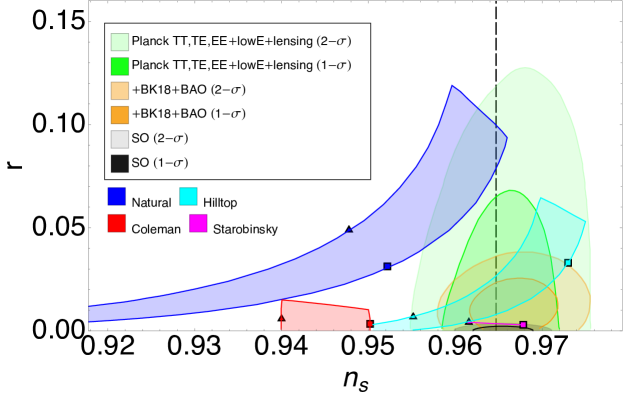
Figure 7: Illustration of $n_{s}-r$ predictions for four inflationary models together with current $1-\sigma$ and $2-\sigma$ best-fit contour from Planck2018 (green shaded region), Planck2018+Bicep3+Keck Array2018 (yellow shaded region) and future CMB observation (SO) with black shaded region.

Appendix B

As mentioned previously, the potential for H-I (Eq. (17)) is not bounded from below. Introducing other term to the potential to stabilize the potential of Eq. (17) affects the $n_{s},r$ predictions of H-I except for the scenario where $v<M_{P}$, where additional term $\propto\phi/v$ can be introduced in the potential . Nevertheless, for such scenario, predicted value of $n_{s}$ even for ${\cal N}_{\text{CMB}}=60$ is less ($n_{s}=0.95$) compared to best-fit $1-\sigma$ contour from CMB data Kallosh:2019jnl ; Kallosh:2019hzo ; Kallosh:2021mnu . To resolve these issues, the regularized form of the H-I (although this form of hilltop potential lacks significant theoretical motivation in contrast to the form of Eq. (17)) has been suggested for $v\gtrsim M_{P}$ as Kallosh:2019jnl

$$V(\phi)=\Lambda_{H}^{4}\quantity[1-\quantity(\frac{\phi}{v})^{4}]^{2}\,.$$ (46)

We have considered $n_{s},r$ predictions of Regularized Hilltop inflation and also C-I for $m\gtrsim M_{P}$ for the completeness of our discussion, and displayed it in the left panel of Fig. 8 as cyan-colored and red-colored regions for ${\cal N}_{\text{CMB}}=50-60$ (line with a triangle and line with a square correspond to ${\cal N}_{\text{CMB}}=50$ and ${\cal N}_{\text{CMB}}=60$). Both of these inflationary models (regularized Hilltop and CW for $f>M_{P}$) predicts $n_{s},r$ values even within $1-\sigma$ best-fit contour from the analysis of Planck2015+Bicep2-Keck Array2015. Interestingly, these two inflationary models also predict $n_{s},r$ values that fall inside $2-\sigma$ CL of the best-fit contour from Guo:2017qjt with best-fit value of $\Delta N_{\mathrm{eff}}=0.254$. The maximum value of $r$ predicted by regularized Hilltop inflationary model used on the left panel is $r=0.158$ (for ${\cal N}_{\text{CMB}}=50$) which is also the same as the maximum value of $r$ considered for CW inflation. The horizontal olive-colored stripe on the right panel of Fig. 8 indicates the range of the value of $r\lesssim 0.158$. The $r-B_{X}$ best-fit contours on the background of the right panel of Fig. 8 are from Ref. DiValentino:2016ucb , as depicted already in Fig. 3. Since $B_{X}\gtrsim 0.02$ and $B_{X}\gtrsim 0.05$ is needed for both regularized Hilltop and C-I inflation to be within at least $68\%$ of CL‘TTTEEE+tau’ and ‘TTTEEE+lowTEB+BKP’ datasets, we conclude that $X$ produced from the decay of inflaton during reheating and contributing solely and completely to $\Delta N_{\mathrm{eff}}$ are simultaneously compatible for these two inflationary scenarios.

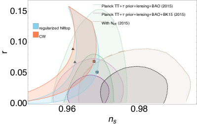
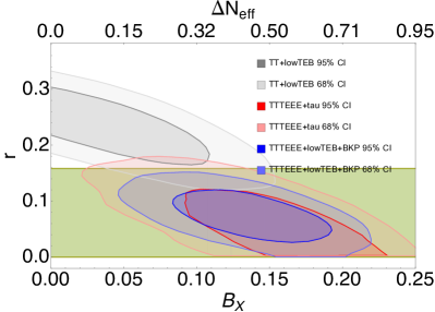
Figure 8: Left panel: illustration of $n_{s}-r$ predictions for regularized Hilltop inflation (Eq. (46)) and C-I inflationary model (Eq. (19)) but for $f\gtrsim M_{P}$ together with $1-\sigma$ and $2-\sigma$ contour from Planck2015, and Planck2015+Bicep2-Keck Array2015 and bound from analysis where $\Delta N_{\mathrm{eff}}$ is treated as a variable from Guo:2017qjt ; Kannike:2018zwn , as described in Fig. 1. Right panel: olive-green shaded region shows the allowed region of $r$ for regularized Hilltop/ C-I (with $f\gtrsim M_{P}$) inflationary models. Additionally, the best fit contour on $(r,B_{X})$ plane in the background is also depicted from Ref. DiValentino:2016ucb , as mentioned in Fig. 3.

Appendix C

Here, we consider that $X$ is a scalar particle $\varphi$ which is produced through $\phi\phi\to\varphi\varphi$ interaction channel. Accordingly, based on Eq. 41, the reaction rate between $\phi$ and $X$-particles can be written as Drewes:2019rxn ; Garcia:2020wiy

$$\Gamma_{\phi\phi\to\varphi\varphi}=\frac{\lambda_{22,\varphi}^{2}\,\left<\phi\right>^{2}}{256\pi\,m_{\phi}}=\frac{\lambda_{22,\varphi}^{2}\,\rho_{\phi}}{128\pi\,m_{\phi}^{3}}\,,\qquad \left(\text{If}\,X\equiv\varphi,\,\text{and}\,\phi\phi\to\varphi\varphi\right)\,.$$ (47)

Then $\Gamma_{\phi}=\Gamma_{\phi\to hh}+\Gamma_{\phi\phi\to\varphi\varphi}$. Since we consider the scenario where the potential of inflaton about the minimum is quadratic during reheating, $m_{\phi}$ is independent of time. However, $\rho_{\phi}$ and, consequently, $\Gamma_{\phi\phi\to\varphi\varphi}$, both evolve with time Garcia:2020wiy . The Boltzmann equations (Eqs. 27, 28 and 29) and Friedman equation (Eq. 30) can be expressed using rescaled dimensionless variables as follows

$$\frac{\differential P}{\differential\tau}+3\,\overline{H}\,P=-\gamma\left(1+r_{\lambda}\,R\right)\,P\,,$$ (48)

$$\frac{\differential R}{\differential\tau}+4\,\overline{H}\,R=\gamma\,P\,,$$ (49)

$$\frac{\differential{\cal X}}{\differential\tau}+4\,\overline{H}\,{\cal X}=\gamma\,r_{\lambda}\,R\,P\,,$$ (50)

$$\overline{H}^{2}=P+R+{\cal X}\,,$$ (51)

where $\tau=t\,{\cal H}_{I}\,,\overline{H}={\cal H}/{{\cal H}_{I}}\,,{\cal H}_{I}^{2}=\quantity({1}/{3M_{P}^{2}})\Phi_{I}\,,P={\rho_{\phi}}/{\Phi_{I}}\,,R={\rho_{\rm rad}}/{\Phi_{I}}\,,{\cal X}={\rho_{X}}/{\Phi_{I}}\,,\gamma={\Gamma_{\phi\to{hh}}}/{{\cal H}_{I}}$. Here, we assume that ${\rho_{\rm rad}}=\rho_{X}=0$ at the onset of the reheating era, with $\Phi_{I}$ denoting the energy density of inflation and ${{\cal H}_{I}}$ representing the value of Hubble parameter at the beginning of reheating. The dimensionless parameter $r_{\lambda}$ is defined as

$$r_{\lambda}=\frac{1}{16\,m_{\phi}^{4}}\frac{\lambda_{22,\varphi}^{2}}{\lambda_{12,H}^{2}}\,\Phi_{I}\,.$$ (52)

In this work, we assume $r_{\lambda}<1$ to avoid the universe being dominated by dark sector particles. By solving Eqs. 48, 49, 50 and 51 and substituting the results into Eq. 32 we obtain the variation of $\Delta N_{\mathrm{eff}}$ with respect to $r_{\lambda}$, considering three different values of $\gamma/\overline{H}$, as depicted in Fig. Fig. 9. From Fig. 9, we conclude that the contribution of scalar BSM particles in $\Delta N_{\mathrm{eff}}$ is very small when $\varphi$ is produced via Eq. 41 rather than Eq. 37. This is because, as the reheating phase progresses, the reaction rate, and therefore $\Gamma_{\phi\phi\to\varphi\varphi}/\Gamma_{\phi\to hh}$, decreases with $\rho_{\phi}$. Due to the same reason, contribution to $\Delta N_{\mathrm{eff}}$ in this scenario ($\phi\phi\to\varphi\varphi$) depends on $\gamma/\overline{H}$ in contrary to $\phi\to\varphi\varphi$ or other interaction channels mentioned earlier (LABEL:{Eq:DecayToFermion}, 38 and 39). The decrease of $\Delta N_{\mathrm{eff}}$ for smaller values of $r_{\lambda}$ is attributed to the same reason observed in the decrease of $\Delta N_{\mathrm{eff}}$ with $B_{X}$ in Fig. 2, which is smaller fraction of $\rho_{\phi}$ being converted to $\rho_{X}$ with smaller values of $r_{\lambda}$.

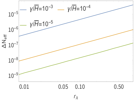
Figure 9: Variation of $\Delta N_{\mathrm{eff}}$ versus $r_{\lambda}$ for three different values of $\gamma/\overline{H}$ for a scalar BSM particle ($\varphi$) contributing to $\Delta N_{\mathrm{eff}}$ and produced via Eq. 41. Contribution to $\Delta N_{\mathrm{eff}}$ decreases with smaller values of both $\gamma/\overline{H}$ and $r_{\lambda}$.

Appendix D

Here, we discuss the conditions, e.g. ranges of the couplings mentioned in Eq. 33, for which our assumption that DR particles are not thermalized with the radiation bath, remains valid. More precisely, we explore the conditions wherein these particles cannot attain kinetic equilibrium with SM Higgs via inflaton exchange diagrams. Let us begin by considering 2-to-2 scattering of DR particles with inflaton as the mediator. The reaction rate (per Higgs particle) is given by

$$\Gamma_{SC}=\expectationvalue{\sigma\,\absolutevalue{v_{\rm rel}}}\,n_{\text{DR}}=\sigma\,\absolutevalue{v_{\rm rel}}\,n_{\text{DR}}\,,$$ (53)

where $n_{\text{DR}}$ is the number density of DR particles, $\absolutevalue{v_{\rm rel}}$ represents the absolute value of the relative velocity between projectile and target particles, and the brackets denote averaging over the phase space. The rightmost equality holds based on our assumption that cross-section $\sigma$ is independent of $v_{\rm rel}$. During the reheating era, we can assume $T\gg M_{H}$, where $M_{H}$ is the mass ($\approx 125\,\text{GeV}$) of SM Higgs particles. Therefore, thermal Higgs particles are relativistic at that time with energy $\approx T$. Furthermore, DR particles are expected to possess considerably low masses to contribute to $\Delta N_{\mathrm{eff}}$. We can also assume that DR particles produced from the decay of inflaton, are also relativistic during the epoch we are interested. Since, DR particles are non-thermal, their temperature need not necessarily align with that of SM Higgs i.e. $T$. Nevertheless, we can approximate that energy of DR particles $\sim{\cal O}\quantity(T)$. Therefore, $\absolutevalue{v_{\rm rel}}\sim 1$ and $n_{\text{DR}}\sim T^{3}$ Dolgov:2009zj . For 2-to-2 scattering process, the total cross-section in center-of-mass frame

$$\sigma\sim\int\frac{\overline{\absolutevalue{{\cal M}}^{2}}}{(E_{1}+E_{2})^{2}}\frac{\absolutevalue{{\bf p}_{f}}}{\absolutevalue{{\bf p}_{i}}}\,\differential\Omega\,,$$ (54)

where $\quantity(E_{1}+E_{2})$ is the sum of the energies of the incoming particles, $\absolutevalue{{\bf p}_{f}}$ is the magnitude of the 3-momentum for either of the outgoing particles, and $\absolutevalue{{\bf p}_{i}}$ is the magnitude of 3-momentum for either of the incoming particles, ${\cal M}$ stands for the Feynman amplitude with the over-line indicating an average taken over unmeasured spins or polarization states of the involved particles, and the integration is performed over solid angle $\Omega$. Following the aforementioned discussion, we assume $E_{1},E_{2}\sim T$ and $\absolutevalue{{\bf p}_{f}}\sim\absolutevalue{{\bf p}_{i}}$. For the scenario, when DR particles are scalar, and interact with SM Higgs particles with inflaton as the mediator, we get at tree-level

$$\overline{\absolutevalue{{\cal M}}^{2}}\sim\frac{1}{m_{\phi}^{4}}\left(\lambda_{12,H}\,\sigma_{m}\,\lambda_{12,\varphi}\,\sigma^{\prime}_{m}\right)^{2}\,.$$ (55)

For $\sigma_{m}\,,\sigma^{\prime}_{m}\sim m_{\phi}$, and utilizing Eq. 54, we get reaction rate

$$\Gamma_{SC}\sim\left(\lambda_{12,H}\,\lambda_{12,\varphi}\right)^{2}\,T\,.$$ (56)

During reheating era, Hubble parameter can be defined as (such that at $T=T_{\rm RH}$, $\rho_{\phi}=\rho_{\rm rad}$) Garcia:2020eof ; Mambrini:2021zpp

$${\cal H}\sim\frac{T^{4}}{M_{P}T_{\rm RH}^{2}}\,.$$ (57)

Therefore, if $\Gamma_{SC}<{\cal H}$ during reheating, DR cannot achieve thermal equilibrium with SM Higgs via inflaton exchange process. The values of $(\lambda_{12,H},\lambda_{12,\varphi})$ for which $\Gamma_{SC}<{\cal H}$ is maintained, is shown in Fig. 10. The solid lines in Fig. 10 represent ${\cal H}$ calculated from Eq. 57 for two different values of $T_{\rm RH}$: $T_{\rm RH}\sim 10^{4}\,\text{GeV}$ and $T_{\rm RH}\sim 10^{7}\,\text{GeV}$, and the dashed lines correspond to $\Gamma_{SC}$ for different values of $(\lambda_{12,H},\lambda_{12,\varphi})$. From Fig. 10 we conclude that even for $T_{\rm RH}\sim 10^{7}\,\text{GeV}$, along with $(\lambda_{12,H}\lesssim 10^{-9},\lambda_{12,,\varphi}\lesssim 10^{-9})$ thermal equilibrium between scalar DR and SM Higgs particles (via inflaton exchange process) is not feasible. This justifies the range of $(\lambda_{12,H},\lambda_{12,\varphi})$ we have considered (for instance, see Fig. 5). Reheating scenarios where $T_{\rm RH}\gtrsim{\cal O}(10^{7})\,\text{GeV}$ may lead to an excessive production of gravitino Kolb:2003ke . Additionally, several proposed scenarios suggest the plausibility of $T_{\rm RH}$ being $\sim 10^{4}\,\text{GeV}$ or even lower (for example, see Ellis:2021kad,Hannestad:2004px,Refs. Ref. Ellis:2021kad ; Hannestad:2004px ). For higher values of $T_{\rm RH}$, we need to consider smaller values of $(\lambda_{12,H},\lambda_{12,\varphi})$ to ensure that scalar DR particles cannot reach thermal equilibrium with SM Higgs.

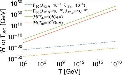
Figure 10: Presentation of representative sets of values for the couplings $(\lambda_{12,H},\lambda_{12,\varphi})$ mentioned in Eqs. 34 and 37, such that scalar DR particles cannot achieve thermal equilibrium with the SM Higgs via inflaton exchange diagram at the tree level. The solid lines correspond to ${\cal H}$ from Eq. 57 for two different values of $T_{\rm RH}$, while the dashed lines correspond to $\Gamma_{SC}$ from Eq. 56, for different values of $(\lambda_{12,H},\lambda_{12,\varphi})$.

For fermionic DR particles (see Eq. 36) and $T\gg M_{H}$, the square of Feynman amplitude of the 2-to-2 scattering process between DR and SM Higgs particles via inflaton exchange diagram is

$$\overline{\absolutevalue{{\cal M}}^{2}}\sim\frac{1}{m_{\phi}^{4}}\left(\lambda_{12,H}\,\sigma_{m}\,y_{\chi}\right)^{2}\,\mathbb{f}_{\chi}\,,$$ (58)

where $\mathbb{f}_{\chi}\sim\sum_{\text{spins}}\left[\bar{u}_{\chi}v_{\bar{\chi}}\right]\left[\bar{u}_{\chi}v_{\bar{\chi}}\right]^{*}\sim 4(p_{\chi}\cdot p_{\bar{\chi}}-m_{\chi}^{2})\sim T^{2}$. Here, $u_{\chi}$, and $v_{\bar{\chi}}$ are Dirac spinors, and $p_{\chi},p_{\bar{\chi}}$ are 4-momenta of fermionic particles. This along with $\sigma_{m}\sim m_{\phi}$, leads to

$$\Gamma_{SC}\sim\frac{1}{m_{\phi}^{2}}\left(\lambda_{12,H}\,y_{\chi}\right)^{2}\,T^{3}\,.$$ (59)

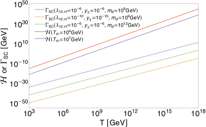
Figure 11: Presentation of representative sets of values for the couplings $(\lambda_{12,H},y_{\chi})$ mentioned in Eqs. 34 and 36, such that fermionic DR particles cannot achieve thermal equilibrium with the SM Higgs via inflaton exchange diagram at the tree level. The solid lines correspond to ${\cal H}$ from Eq. 57 for two different values of $T_{\rm RH}$, while the dashed lines correspond to $\Gamma_{SC}$ from Eq. 59, for different values of $(\lambda_{12,H},y_{\chi})$ and $m_{\phi}$.

Fig. 11 illustrates sample values of $(\lambda_{12,H},y_{\chi})$ for which the condition $\Gamma_{SC}<{\cal H}$ holds. From Fig. 11, we find that achieving thermal equilibrium between DR and SM Higgs particles is not possible for $T_{\rm RH}\sim 10^{7}\,\text{GeV}$, considering values of couplings $(\lambda_{12,H}\lesssim 10^{-6},y_{\chi}\lesssim 10^{-6})$, and $m_{\phi}\sim 10^{9}\,\text{GeV}$. However, higher values of $T_{\rm RH}$ necessitate either smaller values of $(\lambda_{12,H},y_{\chi})$, or a larger value $m_{\phi}$, or both, to ensure that fermionic DR particles cannot reach in thermal equilibrium with SM Higgs via inflaton exchange process.

When DR particles are $U(1)$ gauge boson, and produced for the interaction in Eq. 39, the square of Feynman amplitude of 2-to-2 scattering process between DR and SM Higgs particles via inflaton mediation, is given by

$$\overline{\absolutevalue{{\cal M}}^{2}}\sim\frac{1}{T^{2}}\left(\frac{\lambda_{12,H}\,\sigma_{m}}{m_{\phi}^{2}}\,\frac{g_{\phi\upgamma}}{\Lambda_{m}}\right)^{2}\,\mathbb{f}_{\upgamma}\,,$$ (60)

where $\mathbb{f}_{\upgamma}$ is $\sim(\text{momentum of DR particle})^{4}$. This can be explained as follows: If $A^{\mu}$ is the vector potential of $\upgamma$, and we write it in terms of annihilation ($a_{\lambda_{p}}(\mathbf{k})$) and creation operator $(a_{\lambda_{p}}^{\dagger}(\mathbf{k}))$, then $A^{\mu}$ contains a term $a_{\lambda_{p}}^{\dagger}(\mathbf{k})\,\epsilon_{\lambda_{p}}^{\mu*}\,e^{ikx}$, where the bold symbol denotes 3-vectors, $\epsilon_{\lambda_{p}}^{\mu}$ is the polarization vector, and $\lambda_{p}$ in the subscript is polarization index. Hence, $\partial_{\mu}A^{\nu}$ contains a term $k_{\mu}\,a_{\lambda_{p}}^{\dagger}(\mathbf{k})\,\epsilon_{\lambda_{p}}^{\nu*}\,e^{ikx}$. When we define $F_{\mu\nu}F^{\mu\nu}$ and then, calculate $\absolutevalue{\cal M}^{2}$ we get for our scenario $\mathbb{f}_{\upgamma}\sim T^{4}$. Considering $\Lambda_{m},\sigma_{m}\sim m_{\phi}$, we get

$$\Gamma_{SC}\sim\frac{1}{m_{\phi}^{4}}\left(\lambda_{12,H}\,g_{\phi\upgamma}\right)\,T^{5}\,.$$ (61)

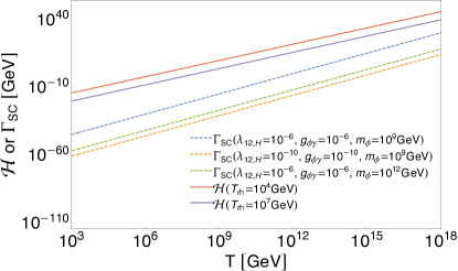
Figure 12: Presentation of representative sets of values for the couplings $(\lambda_{12,H},g_{\phi\upgamma})$ mentioned in Eqs. 34 and 39, such that DR particles, which are $U(1)$ gauge bosons, cannot achieve thermal equilibrium with the SM Higgs via inflaton exchange diagram at the tree level. The solid lines correspond to ${\cal H}$ from Eq. 57 for two different values of $T_{\rm RH}$, while the dashed lines correspond to $\Gamma_{SC}$ from Eq. 61, for different values of $(\lambda_{12,H},y_{\chi})$ and $m_{\phi}$.

Fig. 12 depicts sample values of $(\lambda_{12,H},g_{\phi\upgamma})$ for which the condition $\Gamma_{SC}<{\cal H}$ is upheld. Solid lines in Fig. 12 are used to represent ${\cal H}$ parameter derived from Eq. 57 for two different values of $T_{\rm RH}$: $T_{\rm RH}=10^{4}\,\text{GeV}$ and $T_{\rm RH}\sim 10^{7}\,\text{GeV}$. Moreover, the dashed lines correspond to $\Gamma_{SC}$ for various combinations of values of $(\lambda_{12,H},g_{\phi\upgamma})$ and $m_{\phi}$. Fig. 12 shows that even with $T_{\rm RH}\sim 10^{7}\,\text{GeV}$, and considering $(\lambda_{12,H}\lesssim 10^{-6},g_{\phi\upgamma}\lesssim 10^{-6})$, and $m_{\phi}\sim 10^{9}\,\text{GeV}$, BSM DR particles which are $U(1)$ gauge bosons, cannot establish thermal equilibrium with SM Higgs via 2-to-2 scattering processes with inflaton as the mediator. Reheating scenarios with higher values of $T_{\rm RH}$, requires smaller values of non-thermal condition for DR particles necessitates smaller values of $(\lambda_{12,H},g_{\phi\upgamma})$, or larger $m_{\phi}$, or possibly both, to prevent DR particles from achieving thermal equilibrium with SM Higgs through inflaton mediation scattering processes.

References

- (1)
- (2) A. A. Starobinsky, Phys. Lett. B 91, 99-102 (1980) doi:10.1016/0370-2693(80)90670-X
- (3) K. Sato, Mon. Not. Roy. Astron. Soc. 195, 467-479 (1981) NORDITA-80-29.
- (4) A. H. Guth, Phys. Rev. D 23, 347-356 (1981) doi:10.1103/PhysRevD.23.347
- (5) A. D. Linde, Phys. Lett. B 108, 389-393 (1982) doi:10.1016/0370-2693(82)91219-9
- (6) A. Albrecht and P. J. Steinhardt, Phys. Rev. Lett. 48, 1220-1223 (1982) doi:10.1103/PhysRevLett.48.1220
- (7) A. D. Linde, Phys. Lett. B 129, 177-181 (1983) doi:10.1016/0370-2693(83)90837-7
- (8) A. A. Starobinsky, JETP Lett. 30, 682-685 (1979)
- (9) V. F. Mukhanov and G. V. Chibisov, JETP Lett. 33, 532-535 (1981)
- (10) S. W. Hawking, Phys. Lett. B 115, 295 (1982) doi:10.1016/0370-2693(82)90373-2
- (11) A. A. Starobinsky, Phys. Lett. B 117, 175-178 (1982) doi:10.1016/0370-2693(82)90541-X
- (12) A. H. Guth and S. Y. Pi, Phys. Rev. Lett. 49, 1110-1113 (1982) doi:10.1103/PhysRevLett.49.1110
- (13) J. M. Bardeen, P. J. Steinhardt and M. S. Turner, Phys. Rev. D 28, 679 (1983) doi:10.1103/PhysRevD.28.679
- (14) P. A. R. Ade et al. [Planck], Astron. Astrophys. 571, A1 (2014) doi:10.1051/0004-6361/201321529 [arXiv:1303.5062 [astro-ph.CO]].
- (15) R. Adam et al. [Planck], Astron. Astrophys. 594, A1 (2016) doi:10.1051/0004-6361/201527101 [arXiv:1502.01582 [astro-ph.CO]].
- (16) P. A. R. Ade et al. [BICEP2 and Keck Array], Phys. Rev. Lett. 116, 031302 (2016) doi:10.1103/PhysRevLett.116.031302 [arXiv:1510.09217 [astro-ph.CO]].
- (17) P. A. R. Ade et al. [Planck], Astron. Astrophys. 594, A20 (2016) doi:10.1051/0004-6361/201525898 [arXiv:1502.02114 [astro-ph.CO]].
- (18) J. Martin, C. Ringeval and V. Vennin, Phys. Dark Univ. 5-6, 75-235 (2014) doi:10.1016/j.dark.2014.01.003 [arXiv:1303.3787 [astro-ph.CO]].
- (19) J. Martin, C. Ringeval, R. Trotta and V. Vennin, JCAP 03, 039 (2014) doi:10.1088/1475-7516/2014/03/039 [arXiv:1312.3529 [astro-ph.CO]].
- (20) V. Vennin, J. Martin and C. Ringeval, Comptes Rendus Physique 16, no.10, 960-968 (2015) doi:10.1016/j.crhy.2015.07.007
- (21) E. Menegoni, M. Archidiacono, E. Calabrese, S. Galli, C. J. A. P. Martins and A. Melchiorri, Phys. Rev. D 85, 107301 (2012) doi:10.1103/PhysRevD.85.107301 [arXiv:1202.1476 [astro-ph.CO]].
- (22) M. Archidiacono, E. Calabrese and A. Melchiorri, Phys. Rev. D 84, 123008 (2011) doi:10.1103/PhysRevD.84.123008 [arXiv:1109.2767 [astro-ph.CO]].
- (23) J. Hasenkamp and J. Kersten, JCAP 08, 024 (2013) doi:10.1088/1475-7516/2013/08/024 [arXiv:1212.4160 [hep-ph]].
- (24) L. Ackerman, M. R. Buckley, S. M. Carroll and M. Kamionkowski, Phys. Rev. D 79, 023519 (2009) doi:10.1103/PhysRevD.79.023519 [arXiv:0810.5126 [hep-ph]].
- (25) M. Archidiacono, S. Gariazzo, C. Giunti, S. Hannestad, R. Hansen, M. Laveder and T. Tram, JCAP 08, 067 (2016) doi:10.1088/1475-7516/2016/08/067 [arXiv:1606.07673 [astro-ph.CO]].
- (26) M. Archidiacono, N. Fornengo, S. Gariazzo, C. Giunti, S. Hannestad and M. Laveder, JCAP 06, 031 (2014) doi:10.1088/1475-7516/2014/06/031 [arXiv:1404.1794 [astro-ph.CO]].
- (27) K. J. Bae, H. Baer and E. J. Chun, JCAP 12, 028 (2013) doi:10.1088/1475-7516/2013/12/028 [arXiv:1309.5365 [hep-ph]].
- (28) E. Di Valentino, A. Melchiorri and O. Mena, JCAP 11, 018 (2013) doi:10.1088/1475-7516/2013/11/018 [arXiv:1304.5981 [astro-ph.CO]].
- (29) F. D’Eramo, R. Z. Ferreira, A. Notari and J. L. Bernal, JCAP 11, 014 (2018) doi:10.1088/1475-7516/2018/11/014 [arXiv:1808.07430 [hep-ph]].
- (30) S. Weinberg, Phys. Rev. Lett. 110, no.24, 241301 (2013) doi:10.1103/PhysRevLett.110.241301 [arXiv:1305.1971 [astro-ph.CO]].
- (31) E. Calabrese, D. Huterer, E. V. Linder, A. Melchiorri and L. Pagano, Phys. Rev. D 83, 123504 (2011) doi:10.1103/PhysRevD.83.123504 [arXiv:1103.4132 [astro-ph.CO]].
- (32) G. Mangano, G. Miele, S. Pastor and M. Peloso, Phys. Lett. B 534, 8-16 (2002) doi:10.1016/S0370-2693(02)01622-2 [arXiv:astro-ph/0111408 [astro-ph]].
- (33) P. A. Zyla et al. [Particle Data Group], PTEP 2020, no.8, 083C01 (2020) doi:10.1093/ptep/ptaa104
- (34) C. Boehm, M. J. Dolan and C. McCabe, JCAP 12, 027 (2012) doi:10.1088/1475-7516/2012/12/027 [arXiv:1207.0497 [astro-ph.CO]].
- (35) A. Paul, A. Ghoshal, A. Chatterjee and S. Pal, Eur. Phys. J. C 79, no.10, 818 (2019) doi:10.1140/epjc/s10052-019-7348-5 [arXiv:1808.09706 [astro-ph.CO]].
- (36) T. Tram, R. Vallance and V. Vennin, JCAP 01, 046 (2017) doi:10.1088/1475-7516/2017/01/046 [arXiv:1606.09199 [astro-ph.CO]].
- (37) L. Husdal, Galaxies 4, no.4, 78 (2016) doi:10.3390/galaxies4040078 [arXiv:1609.04979 [astro-ph.CO]].
- (38) G. Mangano, G. Miele, S. Pastor, T. Pinto, O. Pisanti and P. D. Serpico, Nucl. Phys. B 729, 221-234 (2005) doi:10.1016/j.nuclphysb.2005.09.041 [arXiv:hep-ph/0506164 [hep-ph]].
- (39) J. J. Bennett, G. Buldgen, M. Drewes and Y. Y. Y. Wong, JCAP 03, 003 (2020) doi:10.1088/1475-7516/2020/03/003 [arXiv:1911.04504 [hep-ph]].
- (40) M. Escudero Abenza, JCAP 05, 048 (2020) doi:10.1088/1475-7516/2020/05/048 [arXiv:2001.04466 [hep-ph]].
- (41) P. F. de Salas and S. Pastor, JCAP 07, 051 (2016) doi:10.1088/1475-7516/2016/07/051 [arXiv:1606.06986 [hep-ph]].
- (42) A. D. Dolgov and M. Fukugita, JETP Lett. 56, 123-126 (1992)
- (43) A. D. Dolgov and M. Fukugita, Phys. Rev. D 46, 5378-5382 (1992) doi:10.1103/PhysRevD.46.5378
- (44) A. D. Dolgov, Phys. Rept. 370, 333-535 (2002) doi:10.1016/S0370-1573(02)00139-4 [arXiv:hep-ph/0202122 [hep-ph]].
- (45) C. Bambi and A. D. Dolgov, Springer, 2015, ISBN 978-3-662-48077-9 doi:10.1007/978-3-662-48078-6
- (46) C. M. Ho and R. J. Scherrer, Phys. Rev. D 87, no.2, 023505 (2013) doi:10.1103/PhysRevD.87.023505 [arXiv:1208.4347 [astro-ph.CO]].
- (47) S. Roy Choudhury, S. Hannestad and T. Tram, JCAP 10, 018 (2022) doi:10.1088/1475-7516/2022/10/018 [arXiv:2207.07142 [astro-ph.CO]].
- (48) K. Abazajian, G. Addison, P. Adshead, Z. Ahmed, S. W. Allen, D. Alonso, M. Alvarez, A. Anderson, K. S. Arnold and C. Baccigalupi, et al. [arXiv:1907.04473 [astro-ph.IM]].
- (49) K. N. Abazajian and J. Heeck, Phys. Rev. D 100, 075027 (2019) doi:10.1103/PhysRevD.100.075027 [arXiv:1908.03286 [hep-ph]].
- (50) X. Luo, W. Rodejohann and X. J. Xu, JCAP 06, 058 (2020) doi:10.1088/1475-7516/2020/06/058 [arXiv:2005.01629 [hep-ph]].
- (51) M. Berbig and A. Ghoshal, JHEP 05, 172 (2023) doi:10.1007/JHEP05(2023)172 [arXiv:2301.05672 [hep-ph]].
- (52) M. Gerbino, E. Grohs, M. Lattanzi, K. N. Abazajian, N. Blinov, T. Brinckmann, M. C. Chen, Z. Djurcic, P. Du and M. Escudero, et al. [arXiv:2203.07377 [hep-ph]].
- (53) N. Aghanim et al. [Planck], Astron. Astrophys. 641, A6 (2020) [erratum: Astron. Astrophys. 652, C4 (2021)] doi:10.1051/0004-6361/201833910 [arXiv:1807.06209 [astro-ph.CO]].
- (54) L. Balkenhol et al. [SPT-3G], Phys. Rev. D 104, no.8, 083509 (2021) doi:10.1103/PhysRevD.104.083509 [arXiv:2103.13618 [astro-ph.CO]].
- (55) J. Delabrouille et al. [CORE], JCAP 04, 014 (2018) doi:10.1088/1475-7516/2018/04/014 [arXiv:1706.04516 [astro-ph.IM]].
- (56) CMB-Bharat Collaboration, http://cmb-bharat.in.
- (57) S. Hanany et al. [NASA PICO], [arXiv:1902.10541 [astro-ph.IM]].
- (58) K. Abazajian et al. [CMB-S4], [arXiv:2203.08024 [astro-ph.CO]].
- (59) N. Sehgal, S. Aiola, Y. Akrami, K. Basu, M. Boylan-Kolchin, S. Bryan, S. Clesse, F. Y. Cyr-Racine, L. Di Mascolo and S. Dicker, et al. [arXiv:1906.10134 [astro-ph.CO]].
- (60) S. Aiola et al. [CMB-HD], [arXiv:2203.05728 [astro-ph.CO]].
- (61) A. Cheek, L. Heurtier, Y. F. Perez-Gonzalez and J. Turner, Phys. Rev. D 106, no.10, 103012 (2022) doi:10.1103/PhysRevD.106.103012 [arXiv:2207.09462 [astro-ph.CO]].
- (62) L. Senatore, doi:10.1142/9789813149441_0008 [arXiv:1609.00716 [hep-th]].
- (63) A. R. Liddle, P. Parsons and J. D. Barrow, Phys. Rev. D 50, 7222-7232 (1994) doi:10.1103/PhysRevD.50.7222 [arXiv:astro-ph/9408015 [astro-ph]].
- (64) B. Ryden, Cambridge University Press, 1970, ISBN 978-1-107-15483-4, 978-1-316-88984-8, 978-1-316-65108-7 doi:10.1017/9781316651087
- (65) A. Riotto, ICTP Lect. Notes Ser. 14, 317-413 (2003) [arXiv:hep-ph/0210162 [hep-ph]].
- (66) D. H. Lyth, [arXiv:astro-ph/9312022 [astro-ph]].
- (67) H. G. Lillepalu and A. Racioppi, [arXiv:2211.02426 [astro-ph.CO]].
- (68) D. Baumann, Cambridge University Press, 2022, ISBN 978-1-108-93709-2, 978-1-108-83807-8 doi:10.1017/9781108937092
- (69) A. Racioppi and M. Vasar, Eur. Phys. J. Plus 137, no.5, 637 (2022) doi:10.1140/epjp/s13360-022-02853-x [arXiv:2111.09677 [gr-qc]].
- (70) P. A. R. Ade et al. [Planck], Astron. Astrophys. 594, A13 (2016) doi:10.1051/0004-6361/201525830 [arXiv:1502.01589 [astro-ph.CO]].
- (71) P. A. R. Ade et al. [BICEP2 and Keck Array], Phys. Rev. Lett. 121, 221301 (2018) doi:10.1103/PhysRevLett.121.221301 [arXiv:1810.05216 [astro-ph.CO]].
- (72) Y. Akrami et al. [Planck], Astron. Astrophys. 641, A10 (2020) doi:10.1051/0004-6361/201833887 [arXiv:1807.06211 [astro-ph.CO]].
- (73) G. Barenboim, P. B. Denton and I. M. Oldengott, Phys. Rev. D 99, no.8, 083515 (2019) doi:10.1103/PhysRevD.99.083515 [arXiv:1903.02036 [astro-ph.CO]].
- (74) R. Y. Guo and X. Zhang, Eur. Phys. J. C 77, no.12, 882 (2017) doi:10.1140/epjc/s10052-017-5454-9 [arXiv:1704.04784 [astro-ph.CO]].
- (75) K. Kannike, A. Kubarski, L. Marzola and A. Racioppi, Phys. Lett. B 792, 74-80 (2019) doi:10.1016/j.physletb.2019.03.025 [arXiv:1810.12689 [hep-ph]].
- (76) N. Aghanim et al. [Planck], Astron. Astrophys. 594, A11 (2016) doi:10.1051/0004-6361/201526926 [arXiv:1507.02704 [astro-ph.CO]].
- (77) P. A. R. Ade et al. [BICEP2 and Planck], Phys. Rev. Lett. 114, 101301 (2015) doi:10.1103/PhysRevLett.114.101301 [arXiv:1502.00612 [astro-ph.CO]].
- (78) N. Aghanim et al. [Planck], Astron. Astrophys. 596, A107 (2016) doi:10.1051/0004-6361/201628890 [arXiv:1605.02985 [astro-ph.CO]].
- (79) K. Freese, J. A. Frieman and A. V. Olinto, Phys. Rev. Lett. 65, 3233-3236 (1990) doi:10.1103/PhysRevLett.65.3233
- (80) N. K. Stein and W. H. Kinney, JCAP 01, no.01, 022 (2022) doi:10.1088/1475-7516/2022/01/022 [arXiv:2106.02089 [astro-ph.CO]].
- (81) A. Mazumdar, S. Mohanty and P. Parashari, Phys. Rev. D 101, no.8, 083521 (2020) doi:10.1103/PhysRevD.101.083521 [arXiv:1911.08512 [astro-ph.CO]].
- (82) A. De Felice and S. Tsujikawa, Living Rev. Rel. 13, 3 (2010) doi:10.12942/lrr-2010-3 [arXiv:1002.4928 [gr-qc]].
- (83) Y. Aldabergenov, R. Ishikawa, S. V. Ketov and S. I. Kruglov, Phys. Rev. D 98, no.8, 083511 (2018) doi:10.1103/PhysRevD.98.083511 [arXiv:1807.08394 [hep-th]].
- (84) J. E. Kim, H. P. Nilles and M. Peloso, JCAP 01, 005 (2005) doi:10.1088/1475-7516/2005/01/005 [arXiv:hep-ph/0409138 [hep-ph]].
- (85) K. Kohri, C. M. Lin and D. H. Lyth, JCAP 12, 004 (2007) doi:10.1088/1475-7516/2007/12/004 [arXiv:0707.3826 [hep-ph]].
- (86) L. Boubekeur and D. H. Lyth, JCAP 07, 010 (2005) doi:10.1088/1475-7516/2005/07/010 [arXiv:hep-ph/0502047 [hep-ph]].
- (87) G. Barenboim, E. J. Chun and H. M. Lee, Phys. Lett. B 730, 81-88 (2014) doi:10.1016/j.physletb.2014.01.039 [arXiv:1309.1695 [hep-ph]].
- (88) N. Okada, V. N. Şenoğuz and Q. Shafi, Turk. J. Phys. 40, no.2, 150-162 (2016) doi:10.3906/fiz-1505-7 [arXiv:1403.6403 [hep-ph]].
- (89) R. Kallosh and A. Linde, JCAP 09, 030 (2019) doi:10.1088/1475-7516/2019/09/030 [arXiv:1906.02156 [hep-th]].
- (90) S. Choudhury and S. Pal, Phys. Rev. D 85, 043529 (2012) doi:10.1103/PhysRevD.85.043529 [arXiv:1102.4206 [hep-th]].
- (91) V. F. Shvartsman, Pisma Zh. Eksp. Teor. Fiz. 9, 315-317 (1969)
- (92) AG Doroshkevich and M Yu Khlopov. Physical nature of the hidden mass of the universe. Sov. J. Nucl. Phys.(Engl. Transl.);(United States), 39(4), 1984.
- (93) AG Doroshkevich and M Yu Khlopov. Formation of structure in a universe with unstable neutrinos. Monthly Notices of the Royal Astronomical Society, 211(2):277–282, 1984.
- (94) AG Doroshkevich and M Yu Khlopov. Fluctuations of the cosmic background temperature in unstable-particle cosmologies. Soviet Astronomy Letters, 11:236–238, 1985.
- (95) AG Doroshkevich, AA Klypin, and M Yu Khlopov. Cosmological models with unstable neutrinos. Soviet Astronomy, 32:127, 1988.
- (96) AG Doroshkevich, AA Klypin, and MU Khlopov. Large-scale structure of the universe in unstable dark matter models. Monthly Notices of the Royal Astronomical Society, 239(3):923–938, 1989.
- (97) ZG Berezhiani and M Yu Khlopov. Physics of cosmological dark matter in the theory of broken family symmetry. Sov. J. Nucl. Phys, 52:60, 1990.
- (98) ZG Berezhiani and M Yu Khlopov. Cosmology of spontaneously broken gauge family symmetry with axion solution of strong cp-problem. Zeitschrift für Physik C Particles and Fields, 49:73–78, 1991.
- (99) AS Sakharov and M Yu Khlopov. Horizontal unification as the phenomenology of the theory of’everything’. Yadernaya Fizika, 57(4):690–697, 1994.
- (100) Maxim Khlopov. Fundamental particle structure in the cosmological dark matter. International Journal of Modern Physics A, 28(29):1330042, 2013.
- (101) Z. Sakr, Universe 8, no.5, 284 (2022) doi:10.3390/universe8050284
- (102) D. Aloni, M. Joseph, M. Schmaltz and N. Weiner, [arXiv:2301.10792 [astro-ph.CO]].
- (103) K. Ichikawa, M. Kawasaki, K. Nakayama, M. Senami and F. Takahashi, JCAP 05, 008 (2007) doi:10.1088/1475-7516/2007/05/008 [arXiv:hep-ph/0703034 [hep-ph]].
- (104) K. D. Lozanov, [arXiv:1907.04402 [astro-ph.CO]].
- (105) G. F. Giudice, E. W. Kolb and A. Riotto, Phys. Rev. D 64, 023508 (2001) doi:10.1103/PhysRevD.64.023508 [arXiv:hep-ph/0005123 [hep-ph]].
- (106) M. A. G. Garcia, K. Kaneta, Y. Mambrini and K. A. Olive, JCAP 04, 012 (2021) doi:10.1088/1475-7516/2021/04/012 [arXiv:2012.10756 [hep-ph]].
- (107) M. Drewes, J. U. Kang and U. R. Mun, JHEP 11, 072 (2017) doi:10.1007/JHEP11(2017)072 [arXiv:1708.01197 [astro-ph.CO]].
- (108) R. Jinno, T. Moroi and K. Nakayama, Phys. Rev. D 86, 123502 (2012) doi:10.1103/PhysRevD.86.123502 [arXiv:1208.0184 [astro-ph.CO]].
- (109) B. Barman, N. Bernal, Y. Xu and Ó. Zapata, JCAP 07, no.07, 019 (2022) doi:10.1088/1475-7516/2022/07/019 [arXiv:2202.12906 [hep-ph]].
- (110) E. Di Valentino and F. R. Bouchet, JCAP 10, 011 (2016) doi:10.1088/1475-7516/2016/10/011 [arXiv:1609.00328 [astro-ph.CO]].
- (111) M. Drewes, JCAP 09, 069 (2022) doi:10.1088/1475-7516/2022/09/069 [arXiv:1903.09599 [astro-ph.CO]].
- (112) R. Allahverdi, R. Brandenberger, F. Y. Cyr-Racine and A. Mazumdar, Ann. Rev. Nucl. Part. Sci. 60, 27-51 (2010) doi:10.1146/annurev.nucl.012809.104511 [arXiv:1001.2600 [hep-th]].
- (113) E. Di Valentino and L. Mersini-Houghton, JCAP 03, 002 (2017) doi:10.1088/1475-7516/2017/03/002 [arXiv:1612.09588 [astro-ph.CO]].
- (114) K. Freese and W. H. Kinney, JCAP 03, 044 (2015) doi:10.1088/1475-7516/2015/03/044 [arXiv:1403.5277 [astro-ph.CO]].
- (115) G. Panotopoulos, Astropart. Phys. 128, 102559 (2021) doi:10.1016/j.astropartphys.2021.102559
- (116) K. Dimopoulos, C. Owen and A. Racioppi, Astropart. Phys. 103, 16-20 (2018) doi:10.1016/j.astropartphys.2018.06.002 [arXiv:1706.09735 [hep-ph]].
- (117) A. Ghoshal, D. Nanda and A. K. Saha, [arXiv:2210.14176 [hep-ph]].
- (118) N. Aghanim et al. [Planck], Astron. Astrophys. 641, A6 (2020) [erratum: Astron. Astrophys. 652, C4 (2021)] doi:10.1051/0004-6361/201833910 [arXiv:1807.06209 [astro-ph.CO]].
- (119) R. Kallosh and A. Linde, Phys. Rev. D 100, no.12, 123523 (2019) doi:10.1103/PhysRevD.100.123523 [arXiv:1909.04687 [hep-th]].
- (120) A. D. Dolgov, Phys. Atom. Nucl. 73, 815-847 (2010) doi:10.1134/S1063778810050091 [arXiv:0907.0668 [hep-ph]].
- (121) R. Kallosh and A. Linde, JCAP 12, no.12, 008 (2021) doi:10.1088/1475-7516/2021/12/008 [arXiv:2110.10902 [astro-ph.CO]].
- (122) M. A. G. Garcia, K. Kaneta, Y. Mambrini and K. A. Olive, Phys. Rev. D 101, no.12, 123507 (2020) doi:10.1103/PhysRevD.101.123507 [arXiv:2004.08404 [hep-ph]].
- (123) Y. Mambrini and K. A. Olive, Phys. Rev. D 103, no.11, 115009 (2021) doi:10.1103/PhysRevD.103.115009 [arXiv:2102.06214 [hep-ph]].
- (124) E. W. Kolb, A. Notari and A. Riotto, Phys. Rev. D 68, 123505 (2003) doi:10.1103/PhysRevD.68.123505 [arXiv:hep-ph/0307241 [hep-ph]].
- (125) J. Ellis, M. A. G. Garcia, D. V. Nanopoulos, K. A. Olive and S. Verner, Phys. Rev. D 105, no.4, 043504 (2022) doi:10.1103/PhysRevD.105.043504 [arXiv:2112.04466 [hep-ph]].
- (126) S. Hannestad, Phys. Rev. D 70, 043506 (2004) doi:10.1103/PhysRevD.70.043506 [arXiv:astro-ph/0403291 [astro-ph]].