Relativity and decoherence of spacetime superpositions

Abstract

It is univocally anticipated that in a theory of quantum gravity, there exist quantum superpositions of semiclassical states of spacetime geometry. Such states could arise for example, from a source mass in a superposition of spatial configurations. In this paper we introduce a framework for describing such “quantum superpositions of spacetime states.” We introduce the notion of the relativity of spacetime superpositions, demonstrating that for states in which the superposed amplitudes differ by a coordinate transformation, it is always possible to re-express the scenario in terms of dynamics on a single, fixed background. Our result unveils an inherent ambiguity in labelling such superpositions as genuinely quantum-gravitational, which has been done extensively in the literature, most notably with reference to recent proposals to test gravitationally-induced entanglement. We apply our framework to the the above mentioned scenarios looking at gravitationally-induced entanglement, the problem of decoherence of gravitational sources, and clarify commonly overlooked assumptions. In the context of decoherence of gravitational sources, our result implies that the resulting decoherence is not fundamental, but depends on the existence of external systems that define a relative set of coordinates through which the notion of spatial superposition obtains physical meaning.

I Introduction

The twin discoveries of quantum theory and Einstein’s theory of general relativity revolutionized our understanding of physical reality. Perhaps the most distinctive features of these respective theories are the notions of quantum superposition and spacetime. The former postulates that a quantum system with a distinct set of possible configurations may also exist in a general state featuring many of these configurations “at once.” The latter was Einstein’s geometric interpretation of gravity as the curvature of a pseudo-Riemannian manifold, generated by the presence of mass and energy [1].

The most significant challenge for modern physicists is finding a consistent unification of quantum theory with general relativity. It is univocally anticipated that any theory combining relativistic gravitation with quantum mechanics must be able to describe spacetime as possessing quantum-mechanical degrees of freedom, whose states reside in a complex Hilbert space and may be placed in quantum superpositions of different configurations. Various formal approaches such as the Wheeler-deWitt equation [2, 3] and loop quantum gravity [4, 5, 6] have been developed, which (in principle) allow for such environments to be constructed [7, 8, 9, 10, 11, 12].

In this article, we focus on the fundamental issue underlying many recent studies, namely the physical meaning of “superpositions of spacetime metrics” arising from the spatial superposition of a source mass. Such superposition states are considered in the proposals for possible observations of gravitationally-mediated entanglement  [13, 14], in the context of decoherence that they may induce on quantum systems [15, 16, 17, 18, 19, 20], and the indefinite causal structures they give rise to [21, 22, 23, 24, 25]. Here we demonstrate that any effects emerging due to a spatial superposition of a massive object can be formally reproduced using a single spacetime metric, due to two basic tenets of quantum mechanics and relativity: linearity of quantum theory and invariance of dynamics under general coordinate transformations in general relativity [26]. We show how these basic principles combined lead to the notion of “relativity” of quantum superpositions and to invariance of probabilities in quantum mechanics under quantum transformations between coordinates, i.e. between sets of coordinates associated with the system originally described as in a superposition. This is related to but is conceptually simpler than and distinct from the approach of quantum reference frames [27, 28, 29, 30, 31, 32, 33, 34].

Although many claims have been made that such scenarios represent genuine examples of a quantum-gravitational metric [35, 36, 37, 38, 39, 40] (quantum-gravitational insofar as such solutions cannot be described using the frameworks provided by quantum theory and general relativity, minimally requiring a weak-field formulation of quantum gravity), our result shows that this is not unambiguously true. Just as for classical configurations, where only relative distances between objects are of physical significance, the same is also true for gravitational sources in a superposition of different configurations, where the configuration states are related by a coordinate transformation [41].

To understand the impact of the above result, we apply it in three distinct contexts of recent interest: gravitationally-induced entanglement [35], decoherence of spatial superpositions of black holes [16, 17], and of dark matter [18]. We discuss the implications of our findings for the conclusions that can be drawn from such scenarios and possibilities for lifting the inherent ambiguities by considering superpositions of non-diffeomorphic metrics.

II Results

II.1 Relativity of Quantum Superpositions

Before discussing superpositions of mass configurations sourcing gravity, it is important to clarify the key concepts relevant to that discussion in the general context of superpositions of quantum states, without including any interactions.

General covariance demands that absolute position has no physical meaning [42]. For example, we may consider a scenario with two particles, one localized at some position $x_{1}$ and another at some translated position labeled as $x_{1}+\delta x$. In any translationally invariant theory, this scenario is equivalent to the scenario in which the first particle is assigned a position $x_{1}-\delta x$ and the second one is assigned position $x_{1}$. Any difference between the two scenarios is merely apparent, attributed to a choice of a coordinate system, which emphasises that only relative distances are physically meaningful, with coordinate systems playing a subordinate, rather than fundamental role.

We now outline why this idea, despite intuition, does extend to quantum theory, which we then present rigorously in the next section in the context of superpositions of semiclassical states of spacetime.

Consider a scenario with two particles, where the first is assigned a state $|x\rangle$ corresponding to a position $x$, while the second is in a superposition of positions $(|x+\delta x_{1}\rangle+|x+\delta x_{2}\rangle)/\sqrt{2}$. If indeed only relative distances are physically meaningful in describing the configuration of the particles, then the composite state above, $|x\rangle_{1}(|x+\delta x_{1}\rangle_{2}+|x+\delta x_{2}\rangle_{2})/\sqrt{2}$, would be equivalent to a seemingly different state where the second particle is localized at a position $x$ while the first is in a superposition of translations, so that the two-particle state is $(|x-\delta x_{1}\rangle_{1}+|x-\delta x_{2}\rangle_{1})|x\rangle_{2}$. For each individual amplitude, the two states can be related by a passive translation, represented as a unitary operator $\hat{U}(\delta x_{i})$ that enacts a change of classical coordinates labelling the positions, and thus relabelling the basis states of the particles: $|x\rangle_{1}|x+\delta x_{i}\rangle_{2}=\hat{U}(\delta x_{i})|x-\delta x_{i}\rangle_{1}|x\rangle_{2}$. Crucially, a mapping between the superposition states, denoted simply by $\hat{U}$, also exists:

$$\frac{1}{\sqrt{2}}|x_{1}\rangle_{1}(|x_{1}+\delta x_{1}\rangle_{2}+|x_{1}+\delta x_{2}\rangle_{2})$$

$$\qquad=\frac{\hat{U}}{\sqrt{2}}(|x_{2}-\delta x_{1}\rangle_{1}+|x_{2}-\delta x_{2}\rangle_{1})|x_{2}\rangle_{2},$$ (1)

where $\hat{U}$ is now an operator acting jointly on both particles. While it is uncontroversial such an operator $\hat{U}$ exists and can be seen as change of basis in the two-particle Hilbert space, we argue in the next section that it can also be seen as a quantum change of coordinates–to coordinates that are “in a superposition” of different translations relative to the original coordinate system.

Such an interpretation is consistent with the formal framework provided by quantum reference frames (QRFs), which establishes transformations between reference frames defined by physical degrees of freedom (DoFs); however in the above case we do not need to invoke such additional DoFs. We stress that what Eq. (II.1) represents is that the choice and labelling of basis states for a quantum system is conventional, and we recognise that this freedom to relabel the basis is true for any unitary mapping between different bases, even if no classical coordinate transformation exists that such a unitary represents. We sketch the above discussed interpretation of the unitary implied by Eq. (II.1) as a transformation to coordinates in a “superposition” of translations in Fig. 1.

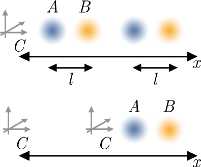
Figure 1: Schematic diagram of an example of a relative state from two different perspectives. In the top subplot, $A$ and $B$ are in a maximally entangled state of their relative distance, with $C$ some “fixed” reference coordinate system through which such distances acquire physical meaning. The bottom subplot is physically equivalent to the top one, where the reference coordinate system $C$ is now in quantum superposition.

II.2 Relativity of Spacetime Superpositions

Here we extend the ideas of the previous section to the case where the masses in question are general relativistic sources of gravity. The results presented here depend only on the linearity of quantum theory and the invariance of physical laws under ordinary coordinate transformations. We first consider a mass in some classical configuration that gives rise to a classical manifold $g$ with coordinates parameterised by $x$. We can assign a semiclassical state to this configuration and the manifold, which can be labelled by $|g(x)\rangle$. Let us now generalise this to a mass in a superposition of two classically distinct configurations $|g_{1}(x_{1})\rangle$, $|g_{2}(x_{2})\rangle$, each of which sources a manifold:

$$|\psi\rangle =\frac{1}{\sqrt{2}}\left(|g_{1}(x_{1})\rangle+|g_{2}(x_{2})\rangle\right),$$ (2)

where $x_{1}$, $x_{2}$ are coordinates associated with the configurations, for example coordinates centered at the position of the mass (we generalise this to arbitrary superposition states in Methods). It is helpful here to conceptualise the mass configuration as being quantum-controlled by an ancillary system that can be prepared and measured in appropriate states. That is, for each state of the control there is an associated mass configuration with a classical manifold and gravitational field, relative to the other quantum DoFs. This is a key assumption that underpins numerous recent investigations in the area of spacetime superpositions, including analyses of gravitationally-induced entanglement proposals [13, 14], spacetime quantum reference frames [28, 29, 30], and decoherence [16, 17, 18].

As discussed, of increasing recent interest are scenarios in which source masses are in a simple superposition of two configurations that differ by a translation and are thus diffeomorphic (related by a coordinate transformation). Formally, a (global) diffeomorphism between the manifolds $M$, $M^{\prime}$ is a smooth map $\varphi:M\to M^{\prime}$ with smooth inverse map $\varphi^{-1}$. Under this definition, the manifolds $M$, $M^{\prime}$ represent the same geometry and are therefore physically indistinguishable. In this section we predominantly focus on superpositions of spacetimes related by a diffeomorphism, returning to general scenarios in the Discussion.

Returning to Eq. (2), it follows that for the manifolds $g_{1}(x_{1})$, $g_{2}(x_{2})$ related by a diffeomorphism, the semiclassical states $|g_{1}(x_{1})\rangle$, $|g_{2}(x_{2})\rangle$ are related by some passive unitary $|g_{1}(x_{1})\rangle=\hat{U}(\delta x)|g_{2}(x_{2})\rangle$ that enacts this diffeomorphism, where $\delta x$ could be some potentially complicated function of the spacetime parameters that characterises the distance between every point between the two coordinate systems $x$, $x^{\prime}$. It is possible to rewrite the state as the unitary $\hat{U}(\delta x)$ that connects the two amplitudes in Eq. (2):

$$|\tilde{\psi}\rangle =\frac{1}{\sqrt{2}}\big{(}\hat{I}+\hat{U}(\delta x)\big{)}|g_{1}(x_{1})\rangle,$$ (3)

where we have utilised the notation $|\tilde{\psi}\rangle\equiv|\psi\rangle$ to distinguish the representation of the state of the spacetime from that of Eq. (2), though as emphasised, the two states are equivalent. This relationship follows from classical general relativity and the basic tenets of quantum theory, namely that symmetries can be represented with unitary operators [43]. We emphasise that the spacetimes are related by a simple relabelling of, for example, the origin of coordinates, and not an active translation of the mass through some pre-existing curved spacetime. Such relabelling of quantum coordinates is consistent with existing frameworks for quantum reference frames and their more recent extensions to curved spacetime [31, 32].

Let us now consider some additional quantum degree of freedom (DoF), $\phi$ in some state $|\phi\rangle$, and a joint initial state of the form,

$$|\psi\rangle =\frac{1}{\sqrt{2}}\left(|g_{1}(x_{1})\rangle+|g_{2}(x_{2})\rangle\right)|\phi\rangle.$$ (4)

The physical system represented by the state $|\phi\rangle$ could be, for example, a quantum field or a particle in first-quantization, or both these interacting with each other–we will consider all of these in the applications of our approach in the next sections and the Methods. The only assumption behind Eq. (4) is that the state of the matter DoFs is uncorrelated with that of the source mass (and thus of the spacetime), but apart from this, is arbitrary. Again, the assumption of an uncorrelated initial state is not necessary, and indeed we will also consider correlated initial states in the Sec. II.4.

Now, in quantum theory, the physically meaningful quantities are probability amplitudes between the states of the system. Let us denote some arbitrary final state $|\Omega\rangle$ and consider their evolution–including free dynamics as well as interactions between the systems–denoted by $\hat{U}$. In general, the time-evolution of the matter DoFs can depend on the state of the source mass which formally can be represented as $\hat{U}_{\mathrm{int.}}=\hat{U}_{1}\otimes|g_{1}\rangle\langle g_{1}|+\hat{U}_{2}\otimes|g_{2}\rangle\langle g_{2}|$, where $\hat{U}_{1}$ and $\hat{U}_{2}$ individually govern the time-evolution of all the DoFs on the respective spacetime and we suppress the symbols $x_{1},x_{2}$ denoting the coordinates associated with a given mass configuration and manifold henceforth as it does not lead to any ambiguity. This gives the general form of the probability amplitude,

$$\langle\Omega|\hat{U}|\psi\rangle =\frac{1}{\sqrt{2}}\big{(}\langle\Omega|\hat{U}_{1}|g_{1}\rangle+\langle\Omega|\hat{U}_{2}|g_{2}\rangle\big{)}|\phi\rangle.$$ (5)

Recall that we can re-express $|g_{2}\rangle$ in terms of the coordinate transformation applied to $|g_{1}\rangle$ enacted by the passive unitary $\hat{U}(\delta x)$. This unitary necessarily acts on the coordinates of all DoFs, and Eq. (5) can be written as

$$\langle\Omega|\hat{U}|\psi\rangle =\frac{1}{\sqrt{2}}\big{(}\langle\Omega|\hat{U}_{1}|g_{1}\rangle|\phi\rangle$$

$$+\langle\Omega|\hat{U}_{2}\hat{U}(\delta x)|g_{1}\rangle|\delta x^{-1}\phi\rangle\big{)},$$ (6)

where the notation $|\delta x^{-1}\phi\rangle$ is understood as the inverse transformation of the coordinates applied to $|\phi\rangle$. Inserting the identity operator expressed as $\hat{I}=\hat{U}(\delta x)\hat{U}^{\dagger}(\delta x)$ in the second term gives,

$$\langle\Omega|\hat{U}|\psi\rangle =\frac{1}{\sqrt{2}}\big{(}\langle\Omega|\hat{U}_{1}|g_{1}\rangle|\phi\rangle$$

$$+\langle\delta x^{-1}\Omega|\hat{U}^{\dagger}(\delta x)\hat{U}_{2}\hat{U}(\delta x)|g_{1}\rangle|\delta x^{-1}\phi\rangle\big{)}.$$ (7)

Importantly, as long as $\hat{U}(\delta x)$ encodes a diffeomorphism, $\hat{U}^{\dagger}(\delta x)\hat{U}_{2}\hat{U}(\delta x)\equiv\hat{U}_{1}$ (enacting a coordinate relabelling of the unitary) and thus

$$\langle\Omega|\hat{U}|\psi\rangle =\frac{1}{\sqrt{2}}\big{(}\langle\Omega|\hat{U}_{1}|g_{1}\rangle|\phi\rangle$$

$$+\langle\delta x^{-1}\Omega|\hat{U}_{1}|g_{1}\rangle|\delta x^{-1}\phi\rangle\big{)}.$$ (8)

Equations (5) and (II.2) describe the same scenario–they demonstrate that in this case, the same dynamics can be interpreted as taking place in space-time that is in superposition, Eq. (5), or in a “single” spacetime where the matter DoFs represented by $\phi$ and the measurements encoded by $|\Omega\rangle$ are correlated accordingly, Eq. (II.2).

This is a key point of this article, and one that is commonly overlooked. So-called “quantum superpositions” of spacetimes can be ambiguous–as in the example given here–and can be re-expressed in terms of modified initial states and measurements of the remaining DoFs, but where the state associated with the source mass, and thus with the spacetime, can be treated as classical. This equivalence between representations is especially important given the recent interest in identifying purportedly quantum-gravitational effects produced by spatial superpositions of a source mass.

As an illustration of this idea, take $\hat{U}(\delta x)$ to be a a simple translation of the coordinates by some distance $\delta x$. Equation (II.2) can thus be written as

$$\langle\Omega|\hat{U}|\psi\rangle =\frac{1}{\sqrt{2}}\big{(}\langle\Omega|\hat{U}_{1}|g_{1}\rangle|\phi\rangle$$

$$\qquad+\langle\Omega-\delta x|\hat{U}_{1}|g_{1}\rangle|\phi-\delta x\rangle\big{)}.$$ (9)

Again, we have here a situation in which all the dynamics and measurements between the considered DoFs occur on a single “fixed” spacetime background described by $|g_{1}\rangle$, compared with Eq. (5) which for this case describes the source mass in a spatial superposition with the distance $\delta x$ in some coordinates; we have sketched this schematically in Fig. 2.

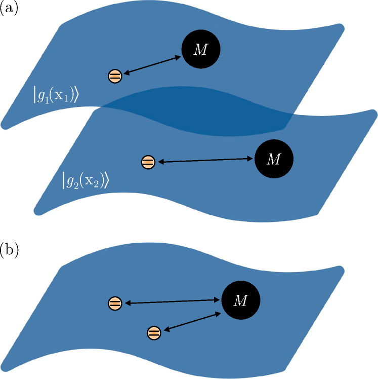
Figure 2: Illustration of how the same scenario viewed from different coordinates acquires the interpretation of (a) superposition of spacetimes, (b) superposition of locations of matter DoFs (e.g. a test particle) with respect to one mass configuration.

The above discussed notion of the relativity of spacetime superpositions should be understood as a statement about the invariance of physical predictions on the choice of coordinates and the related fact that only relative quantities have physical meaning and relevance (e.g. for the strength of an interaction)–in the present context this will mostly refer to relative distances. Recall that a superposition of diffeomorphically related spacetimes can equivalently be represented via suitably adapted states and measurements via dynamics occurring on a single spacetime background.

One can think, however, that once a complete (e.g. interferometric) scenario is considered such a change of representation can no longer be achieved. By the above arguments, this can be done. If in addition the matter DoFs only evolve by a phase like in many recently considered scenarios, even further identifications between apparently different scenarios can be made as follows.

Consider the representation given by Eq. (2), with some additional quantum DoFs coupled to the spacetime i.e. Eq. (4). Time-evolving the system and measuring the source mass in the superposition basis $|\eta\rangle=(|g_{1}\rangle+|g_{2}\rangle)/\sqrt{2}$ gives the final conditional state of the remaining DoFs:

$$\langle\eta|\hat{U}|\psi\rangle =\frac{1}{2}\big{(}\hat{U}_{1}+\hat{U}_{2}\big{)}|\phi\rangle.$$ (10)

Note that the state on which we condition is chosen to be the same as the initial state just for simplicity. However this can be arbitrary, for example imprinted with some relative phase $\varphi$ as in typical interferometric setups. The DoFs described by the state $|\phi\rangle$ evolve in a coherent superposition of “paths” parametrised by the coordinates $x_{1},x_{2}$, associated with the different amplitudes of the spacetime superposition. Probability amplitudes for the remaining DoFs can be obtained by calculating the overlap with some final state $|\Omega\rangle$, giving the probability amplitude $\langle\Omega|\langle\eta|\hat{U}|\psi\rangle$, which explicitly reads

$$\frac{1}{2}\langle\Omega|\big{(}\hat{U}_{1}+\hat{U}_{2}\big{)}|\phi\rangle.$$ (11)

On the other hand, if we adopt the representation given by Eq. (II.2) (for the specific example of a superposition of translations), the amplitude equivalently reads

$$\frac{1}{{2}}\big{(}\langle\Omega|\hat{U}_{1}|\phi\rangle+\langle\Omega-\delta x|\hat{U}_{1}|\phi-\delta x\rangle\big{)},$$ (12)

where we used the fact that the two mass configurations and metrics are macroscopically distinct, meaning $\langle g_{1}(x)|\hat{U}^{\dagger}(\delta x)|g_{1}(x)\rangle=\langle g_{1}(x)|\hat{U}(\delta x)|g_{1}(x)\rangle=0$, and that $\hat{U}^{\dagger}(\delta x)\hat{U}_{1}\hat{U}(\delta x)=\hat{U}_{2}$ by virtue of the fact that $\hat{U}(\delta x)$ encodes a diffeomorphism.

Equation (12) is a formal statement of the fact that a scenario involving quantum systems in a spacetime sourced by a spatial superposition of mass configurations is fully equivalent to a scenario where the particle follows superposed trajectories in one spacetime. The equivalence between the two scenarios can be interpreted as describing the same physical situation simply using two sets of coordinates related by a “superposition” of classical transformations [41], similar to scenarios arising in the context of quantum reference frames [27] operationally established using quantum systems. This general equivalence further implies that probability amplitudes of matter DoFs will be identical in both scenarios (e.g. the transition probability of quantum matter coupled to a quantum field).

The crux of the argument is that only relative configurations between the interacting systems are physically relevant, such as a superposition of two distances between a pair of particles; a global (joint) coordinate transformation enacted on all degrees of freedom is irrelevant. Scenarios where quantum probes are situated on a classical background while the time-evolution occurs in a superposition of trajectories were recently considered in Refs. [44, 45, 46, 47, 48].

Let us take an approximation that two amplitudes of the matter remain orthogonal (e.g. only evolve by a phase as in Refs [13, 14]) which here means that $\langle\Omega-\delta x|\hat{U}_{1}|\phi\rangle=\langle\Omega|\hat{U}_{1}|\phi-\delta x\rangle=0$, so that the above can be equivalently written as

$$\frac{1}{{2}}\big{(}\langle\Omega|+\langle\Omega-\delta x|\big{)}\hat{U}_{1}\big{(}|\phi\rangle+|\phi-\delta x\rangle\big{)}.$$ (13)

This reflects that the scenario (a) in which the source mass is prepared and measured in superposition while the other DoFs evolve in the resulting superposition of metrics is equivalent to the scenario (b) in which the other DoFs are prepared and measured in superposition while the source mass remains in some fixed state sourcing a classical metric.

We conclude this section by mentioning that the formalism presented here has a well-defined non-relativistic limit, in which it can describe matter that sources a Newtonian potential and through this potential interacts with other massive particles. This is of course also true for general relativistic descriptions of a classical metric that reduce to the non-relativistic Newtonian description in such a limit. Such “superpositions of Newtonian potentials,” which have garnered just as much interest as their general relativistic counterparts (see for example Refs [49, 50, 51, 52, 53] and the following section on gravitationally-induced entanglement proposals), are fully characterised by the present framework. We now turn to specific scenarios of practical interest as applications of our results.

II.3 Superposition of Geometries in the Gravitationally-Induced Entanglement Proposals

The previous analysis demonstrated how in general, spacetime superpositions in which the respective amplitudes are related by a diffeomorphism can be re-expressed in terms of a single background spacetime with the states and measurements of the remaining DoFs suitably adapted. This motivates us to revisit the conclusions one can draw concerning quantum gravity from such scenarios.

In this section, we apply our approach and construction to recent proposals by Bose et. al. [13] and Marletto and Vedral [14], which have attracted significant recent interest as presenting possibilities for witnessing the quantization of the gravitational field. These “gravitationally-induced entanglement” (GIE) setups suggest that observing entanglement between two spatially superposed source masses, interacting through the Newtonian potential, is not equivalent to matter interferometry on a fixed background and would provide evidence of the quantum nature of gravity (for example, that entanglement is mediated via gravitons). Here, we focus on a recent interpretation of this argument by Christodolou and Rovelli [35] who argue that such a setup represents a superposition of genuinely distinct spacetime metrics [35].

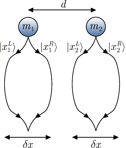
Figure 3: Schematic diagram of the GIE proposal. Each of the states $|x_{i}^{L,R}\rangle$ is assumed to be in a highly localised Gaussian wavepacket such that their overlap is zero.

The GIE proposal is depicted in Fig. 3. Two masses, $m_{1}$ and $m_{2}$, are each prepared and measured in spatial superpostion of freely falling trajectories in the uniform gravitational field of Earth (for example via Stern-Gerlach interferometry techniques). Thus initially, each particle is in a state of the form

$$|\psi_{i}\rangle =\frac{1}{\sqrt{2}}\big{(}|x_{i}^{L}\rangle+|x_{i}^{R}\rangle\big{)},$$ (14)

where $i=1,2$ labels the particles, while the labels $L$, $R$ denote mutually orthogonal eigenstates of the $x$-component of the spin-1/2 particle, controlling the path that each particle takes. For simplicity, we have chosen the separation between the paths, $\delta x$, to be equal for each particle, though the analysis applies for arbitrary separations between any of the branches of the state. Evolution under mutual gravitational interaction for a time $\tau$ entangles the test masses by imparting distance-dependent phases to the components of the superposition.

Christodolou and Rovelli note that immediately after the superpositions are created, we have a product state of the particles and some external metric $|g\rangle$ that has not had time to change appreciably,

$$|\psi\rangle =\frac{1}{2}\big{(}|x_{1}^{L}\rangle+|x_{1}^{R}\rangle\big{)}\big{(}|x_{2}^{L}\rangle+|x_{2}^{R}\rangle\big{)}\otimes|g\rangle,$$

$$=\frac{1}{2}\big{(}|x_{1}^{L},x_{2}^{L}\rangle+|x_{1}^{L},x_{2}^{R}\rangle$$

$$\qquad+|x_{1}^{R},x_{2}^{L}\rangle+|x_{1}^{R},x_{2}^{R}\rangle\big{)}\otimes|g\rangle.$$ (15)

However, once the gravitational disturbance has had time to propagate, each branch of the two-particle state will source, in general, a different metric depending on the relative distance between the particles in that branch:

$$|\psi\rangle \to\frac{1}{2}\big{(}|x_{1}^{L},x_{2}^{L},g_{LL}\rangle+|x_{1}^{L},x_{2}^{R},g_{LR}\rangle$$

$$\qquad+|x_{1}^{R},x_{2}^{L},g_{RL}\rangle+|x_{1}^{R},x_{2}^{R},g_{RR}\rangle\big{)}$$ (16)

where $g_{ij}$, $i,j=R,L$ denote the respective metrics. They further argue that such a scenario no longer represents a semiclassical spacetime but a genuine superposition of metrics. This is true when referring to the metric generated by both particles, each in superposition.

However the GIE proposal does not depend on a geometry that is sourced by both particles. The result of the proposed interferometric measurements depend on the gravitational interaction between the two particles. Thus, the metric involved can be interpreted as that sourced by, say, particle $i=1$ (this choice being arbitrary), and despite the point made by Christodolou and Rovelli, the proposed setup of Fig. 3 can be reinterpreted as an interference experiment on classical space-time, where a ‘source’ particle follows a fixed trajectory while the other undergoes a suitably adapted interference experiment, using our framework developed in the earlier section.

To see this explicitly, note that the states $|\psi_{i}^{L}\rangle$, $|\psi_{i}^{R}\rangle$ can be related by a unitary operator $\hat{U}(\delta x)$ implementing a translation by the distance $\delta x$, so that we can express Eq. (II.3) as

$$|\psi\rangle =\frac{1}{2}\big{(}|x_{1}^{L},x_{2}^{L}\rangle+|x_{1}^{L},x_{2}^{R}\rangle+\hat{U}(\delta x)|x_{1}^{L},x_{2}^{L}-\delta x\rangle\vphantom{\frac{1}{2}}$$

$$\qquad+\hat{U}(\delta x)|x_{1}^{L},x_{2}^{R}-\delta x\rangle\big{)}.\vphantom{\frac{1}{2}}$$ (17)

In the GIE proposal, after some interval of time-evolution each mass is measured in a superposition, and so the relevant amplitude is $\langle\eta|\hat{U}|\psi\rangle$ where $|\eta\rangle=|\eta_{1}\rangle\otimes|\eta_{2}\rangle$.

Using our general result, leading to Eq. (12), we obtain

$$\langle\eta|\hat{U}|\psi\rangle =\frac{1}{2}\big{(}\langle\eta_{1}|\langle\eta_{2}|\hat{U}|x_{1}^{L},x_{2}^{L}\rangle\vphantom{\frac{1}{2}}$$

$$+\langle\eta_{1}|\langle\eta_{2}|\hat{U}|x_{1}^{L},x_{2}^{R}\rangle\vphantom{\frac{1}{2}}$$

$$+\langle\eta_{1}-\delta x|\langle\eta_{2}-\delta x|\hat{U}|x_{1}^{L},x_{2}^{L}-\delta x\rangle\vphantom{\frac{1}{2}}$$

$$+\langle\eta_{1}-\delta x|\langle\eta_{2}-\delta x|\hat{U}|x_{1}^{L},x_{2}^{R}-\delta x\rangle\big{)}\vphantom{\frac{1}{2}}$$ (18)

where we have used the fact that GIE assumes an interaction given by $\hat{U}=\int\mathrm{d}x_{1}\mathrm{d}x_{2}\exp(-it\frac{Gm_{1}m_{2}}{|\hat{x}_{1}-\hat{x}_{2}|})|x_{1}\rangle\langle x_{1}|\otimes|x_{2}\rangle\langle x_{2}|$, i.e. the Newtonian potential depending on the distance $x_{1}-x_{2}$ between each of the respective branches of the superposition, which is explicitly invariant under passive translations (i.e. translations of both coordinates).

To finalise our argument, note that this interaction allows us to consider either of the particles as the source mass of the potential at the location of the other particle (if there were a third system considered, e.g. a small test mass, then the metric in the vicinity of that mass would be sourced by both particles $i=1,2$. However in the present scenario, only two particles are involved). Considering the particle $i=1$ as the source, the associated metric in the above is fixed (defined by the position of that particle) and thus allows us to interpret the scenario as the evolution of the second particle, which is in a superposition of four amplitudes, taking place on a single spacetime. This becomes particularly clear when including the assumption made in this scenario, that the states only evolve by a phase while the distance between the particles remains unchanged, and that the measurements are performed in a superposition of the paths, i.e. $|\eta_{i}\rangle=(|x_{i}^{L}\rangle+|x_{i}^{R}\rangle)/\sqrt{2}$. These two together mean that in the original formulation, the relevant amplitude is

$$\langle\eta|\hat{U}|\psi\rangle=\frac{1}{4}\sum_{n,m}\langle x_{1}^{n},x_{2}^{m}|\hat{U}|x_{1}^{n},x_{2}^{m}\rangle,$$ (19)

where $n,m=L,R$ implies a sum over the four amplitudes, while using our result in Eq. (II.3), the same amplitude reads

$$\langle\eta|\hat{U}|\psi\rangle=\langle\tilde{x}_{2}|\langle x_{1}^{L}|\hat{U}|x_{1}^{L}\rangle|\tilde{x}_{2}\rangle,$$ (20)

where $|\tilde{x}_{2}\rangle:=(|x_{2}^{L}\rangle+|x_{2}^{L}-\delta x\rangle+|x_{2}^{R}\rangle+|x_{2}^{R}-\delta x\rangle)/\sqrt{4}$. Clearly we can write this as $\langle\tilde{x}_{2}|\hat{U}_{L}|\tilde{x}_{2}\rangle$ where $\hat{U}_{L}=\int\mathrm{d}x_{2}\exp(-it\frac{Gm_{1}m_{1}}{|x_{1}^{L}-\hat{x}_{2}|})|x_{2}\rangle\langle x_{2}|$ is the gravitational potential sourced by particle $1$ positioned at $x_{1}^{L}$ and experienced by particle $2$.

The calculation above shows that GIE, originally explained as due to a quantum superposition of gravitating source masses, can be explained in terms of a test mass in a classical potential sourced by the other mass. Thus, independently of any other considerations, there is an inherent ambiguity in the interpretation of such experiments as testing quantum features of gravitational degrees of freedom. Indeed, using linearity of quantum theory the same amplitude is obtained from the expression Eq. (20) in which the gravitational field only features as an external (classical) potential. We stress that this ambiguity is present because in the considered scenario only relative distances between the particles play a role in determining the final probability, and not their absolute locations relative to, say, the laboratory reference frame.

Consequently, the interpretation that the initial state Eq. (II.3) evolves into Eq. (II.3) describing an entangled state of semiclassical spacetime metrics, while correct, is not required to predict the amplitude of interest in this proposal. Instead, the result of the experiment can be adequately described in terms of a superposition of distances between masses where the one designated as the source is fixed, and consequently the spacetime is fixed. This highlights again the inherent ambiguity in the notion of “spacetime superposition” if the superposed amplitudes differ by a diffeomorphism (or any symmetry of the dynamics).

Removing the above ambiguity requires superpositions of non-diffeomorphic metrics. By definition such metrics are not related by any change of coordinates, since they effectively give rise to unique solutions to the Einstein field equations. It then follows that the prior analysis, in which various amplitudes in superposition could be related by unitaries representing a general coordinate transformation, is no longer applicable. In such cases, the superposition of geometries that arises is unambiguously quantum-gravitational, insofar as the resulting metrics associated with different amplitdues cannot be re-expressed as a single classical metric with suitably transformed dynamics and measurement bases for the remaining DoFs. Applied to the GIE proposals, this could involve atoms that are prepared in a superposition of energy eigenstates [54], with each eigenstate generating a different curvature. Related examples that have been studied in the literature include a black hole [55, 56] or dark matter clump [18] in a superposition of masses, and an expanding universe in a superposition of expansion rates [47].

II.4 Apparent Decoherence of Spacetime Superpositions

In the previous section, we showed how the linearity of quantum theory and the fact that the notion of position is a relative one (only relative distances between systems are physically meaningful) leads to the relativity of spacetime superpositions, and we demonstrated that this has significant implications for the interpretation of scenarios that appear to give rise to quantum superpositions of geometries. In this section, we apply our approach to scenarios exploring the phenomenon of decoherence. We show how following a common approach may lead to different conclusions about the decoherence of a mass configuration, depending on how one defines the coordinate system to describe the configuration.

Let us consider for example, the case of a black hole at some position and its Hawking radiation, described by the state $|\chi_{i}\rangle\equiv|\chi_{i}(x_{i})\rangle$ with $x_{i}$ being the position of the black hole. A black hole in superposition of different positions $x_{1}$ and $x_{2}$ would evolve into an entangled state

$$|\psi\rangle =\frac{1}{\sqrt{2}}\left(|x_{1},\chi_{1}\rangle+|x_{2},\chi_{2}\rangle\right),$$ (21)

since a black hole cannot be ultimately isolated from its Hawking radiation, and we have assumed the shorthand $|x_{i},\chi_{i}\rangle\equiv|x_{i}\rangle\otimes|\chi_{i}\rangle$. Upon tracing out the radiation degrees of freedom from the state in Eq. (21), one finds

$$\mathrm{Tr}_{\chi}|\psi\rangle\langle\psi| =\frac{1}{2}\begin{pmatrix}1&|\nu|^{2}\\ |\nu|^{2}&1\end{pmatrix}\to\frac{1}{2}\begin{pmatrix}1&0\\ 0&1\end{pmatrix},$$ (22)

where $\nu=\langle\chi_{1}|\chi_{2}\rangle$ is the overlap between the radiation states associated with the different positions of the black hole. For distinguishable states of the radiation, over time the off-diagonal elements of the reduced density matrix will become suppressed, leaving a classical mixture of the two locations of the black hole. This has been argued to lead to fundamental decoherence [16, 17, 20] , due to the above mentioned fact that a black hole cannot be isolated from its Hawking radiation.

However based on the framework introduced thus far, the relevant question is, with respect to what physical system is the black hole superposed? As we have discussed, the use of physical systems that can interact with the source mass and measurements of final probability amplitudes is crucial for understanding the physical implications of scenarios involving superpositions of spacetime metrics. For example, choosing coordinates whose origin is defined as the location of the black hole, Eq. (21) by construction becomes a product state of the black hole and its radiation,

$$|\psi\rangle =|x_{1},\chi_{1}\rangle,$$ (23)

from which one would not deduce decoherence. Based on our framework for the relativity of superpositions, the transformation between Eq. (21) and Eq. (23) involves or acts on all DoFs. The tacit assumption behind Eq. (22) is that in computing the overlap $\nu$, one necessarily has access to an uncorrelated measuring device (for example a first-quantised particle) that can probe different spacetime points of the radiation field $\chi(x)$ [57, 58].

To see this, it is instructive to consider probability amplitudes that are obtained by coupling a measuring device (or devices) that are perfectly correlated with the position of the black hole. The measuring device may function as a proxy for arbitrary matter DoFs that are correlated with the black hole-radiation system. We can take the state of this device to be

$$|\Omega\rangle =\frac{1}{\sqrt{2}}\left(|x_{1},\Omega_{1}\rangle+|x_{2},\Omega_{2}\rangle\right).$$ (24)

In this scenario the relative distance between the measuring device and the black hole is identical in each branch of the superposition. For ease of comparison, let us consider the approach of Ref. [16], which models the black hole as a dielectric sphere that interacts with (isotropically) scattered and emitted (Hawking) photons. Time-evolving the state with the quantum-controlled unitary $\hat{U}=\sum_{i}\hat{U}_{i}|x_{i},\chi_{i}\rangle\langle x_{i},\chi_{i}|$ gives

$$\hat{U}\hat{\rho}\hat{U}^{\dagger} =\frac{1}{2}\sum_{i,j}\hat{U}_{i}|x_{i},\chi_{i}\rangle\langle\chi_{j},x_{j}|\hat{U}_{j}^{\dagger},$$ (25)

where the sum runs over $i,j=1,2$. Crucially, the radiation states are here correlated with the black hole position, and hence the relative distance between these subsystems is fixed in either branch of the superposition. Measuring the system in the correlated state given by Eq. (24) yields

$$\langle\Omega|\hat{U}\hat{\rho}\hat{U}^{\dagger}|\Omega\rangle\vphantom{\frac{1}{2}}$$

$$\>\>\>=\frac{1}{4}\big{(}\langle\Omega_{1},x_{1}|\hat{U}_{1}|x_{1},\chi_{1}\rangle\langle\chi_{1},x_{1}|\hat{U}_{1}^{\dagger}|x_{1},\Omega_{1}\rangle\vphantom{\frac{1}{2}}$$

$$\>\>\>\qquad+\langle\Omega_{1},x_{1}|\hat{U}_{1}|x_{1},\chi_{1}\rangle\langle\chi_{2},x_{2}|\hat{U}_{2}^{\dagger}|x_{2},\Omega_{2}\rangle\vphantom{\frac{1}{2}}$$

$$\>\>\>\qquad+\langle\Omega_{2},x_{2}|\hat{U}_{2}|x_{2},\chi_{2}\rangle\langle\chi_{1},x_{1}|\hat{U}_{1}^{\dagger}|x_{1},\Omega_{1}\rangle\vphantom{\frac{1}{2}}$$

$$\>\>\>\qquad+\langle\Omega_{2},x_{2}|\hat{U}_{2}|x_{2},\chi_{2}\rangle\langle\chi_{2},x_{2}|\hat{U}_{2}^{\dagger}|x_{2},\Omega_{2}\rangle\vphantom{\frac{1}{2}}\big{)}$$

$$\>\>\>\qquad+\mathrm{orthogonal\>terms}.\vphantom{\frac{1}{2}}$$ (26)

where in the momentum basis, the density matrix for the radiation (correlated with the black hole position) is given by $|\chi_{i}\rangle\langle\chi_{j}|=\int\mathrm{d}^{3}k\frac{p(k)}{4\pi k^{2}}\exp(-i\hat{k}\cdot\hat{x}_{i})|k\rangle\langle k|\exp(i\hat{k}\cdot\hat{x}_{j})$, and $p(k)$ is the probability of emitting a particle with momentum $k$ [16]. The “orthogonal terms” are those that vanish under the assumption that the spacetimes are macroscopically distinct. Utilising the fact that the black hole states (including all additional coupled DoFs, $\phi=\chi,\Omega$) are related via the unitary translation $|x_{2},\phi(x_{2})\rangle=\hat{U}(\delta x)|x_{1},\phi(x_{1})\rangle$, and that $\hat{U}^{\dagger}(\delta x)\hat{U}_{2}\hat{U}(\delta x)\equiv\hat{U}_{1}$, we find that

$$\langle\Omega|\hat{U}\hat{\rho}\hat{U}^{\dagger}|\Omega\rangle =\left|\langle\Omega_{1},x_{1}|\hat{U}_{1}|x_{1},\chi_{1}\rangle\right|^{2}.$$ (27)

This of course, is the standard probability amplitude between the initial and final states $|\chi_{1}\rangle$, $|\Omega_{1}\rangle$, computed on the classical spacetime metric $|x\rangle$ produced by the black hole. The black hole is in a “classical position state” with respect to the correlated measuring device; in principle, this could be extended to all other matter DoFs in the universe. In this scenario, there does not exist an absolute set of relative coordinates with which decoherence can be meaningfully computed, and thus one concludes that there is no decoherence at all.

The alternative scenario is to consider a measuring device that is not initially correlated with the position of the black hole, for example described by the state $|\Omega\rangle=|\Omega_{1}\rangle(|x_{1}\rangle+|x_{2}\rangle)/\sqrt{2}$. In this case,

$$\langle\Omega|\hat{U}\hat{\rho}\hat{U}^{\dagger}|\Omega\rangle\vphantom{\frac{1}{2}}$$

$$\>\>\>=\frac{1}{2}\big{(}\langle\Omega_{1},x_{1}|\hat{U}_{1}|x_{1},\chi_{1}\rangle\langle\chi_{1},x_{1}|\hat{U}_{1}^{\dagger}|x_{1},\Omega_{1}\rangle\vphantom{\frac{1}{2}}$$

$$\qquad+\langle\Omega_{1},x_{2}|\hat{U}_{2}|x_{2},\chi_{2}\rangle\langle\chi_{2},x_{2}|\hat{U}_{2}^{\dagger}|x_{2},\Omega_{1}\rangle\big{)}.\vphantom{\frac{1}{2}}$$ (28)

The conditional state Eq. (II.4) will in general lead to off-diagonal terms given by the overlap between the state of the measurement device and the radiation state $\chi_{2}$, $\langle\Omega_{1}|\chi_{2}\rangle$. It follows that the black hole will decohere over time as information about its position is exchanged through its radiation to the measurement device.

In order to obtain decoherence then, one must necessarily account for the fact that the black hole is not perfectly isolated from external DoFs through which its state is defined. In this sense, decoherence of black holes due to Hawking radiation is not fundamental. Unruh pointed out such examples as demonstrating a “false loss of coherence” [59]. The basic idea is that decoherence is often inferred by virtue of the coupling between a system and its environment, which in this case is represented by the position of the black hole $|x\rangle$ with its radiation field $|\chi(x)\rangle$. However, so long as any changes to the system are made adiabatically, the radiation field is effectively enslaved to the position of the black hole, and hence correlated with the black hole position. If the black hole states are brought back together adiabatically, interference will be observed and coherence is recovered.

II.5 Coherence of Spacetime Superpositions

To conclude, we now demonstrate using our framework how spacetime superpositions do not fully decohere even in circumstances where the presence of additional matter DoFs reveals which-way information about the quantum spacetime. Let us consider for concreteness the case where a probe particle resides outside a black hole in a superposition of relative distances from the horizon. For simplicity we can model the particle as a qubit with internal states $\{|0\rangle,|1\rangle\}$, which interacts with the spacetime superposition through the quantum field $\hat{\phi}$, whose initial state is denoted by $|\phi\rangle$. The evolution of the black hole, quantum field, and matter system takes the form $\hat{U}|\psi\rangle=(\hat{U}_{1}|g_{1}\rangle+\hat{U}_{2}|g_{2}\rangle)|\phi\rangle|0\rangle/\sqrt{2}$. As usual, the interaction takes place in a quantum-controlled superposition of coordinate parametrisations, wherein the individual evolutions depend on the field operator $\hat{\phi}\equiv\hat{\phi}(x_{1}),\hat{\phi}(x_{2})$ on the different manifolds in superposition. We have written the state of the field $|\phi\rangle$ as separable from the control degree of freedom. This is a particular choice following a recent investigation that showed this to be convenient in the case of the (2+1)-dimensional Banados-Zanelli-Teitelboim black hole, where the ground state of the field can be taken to be the anti-de Sitter vacuum state [55]. However we are not constrained by this choice; one could in principle assume the field state to be correlated with the black hole (or the control system correlated with the black hole) as well.

To compute the decoherence of the black hole, we can consider an interferometric setup in which the black hole (or the control system correlated with the black hole) undergoes a Mach-Zehnder-type trajectory with a controllable phase $\varphi$ on one of the arms [21]. Measuring the control in the superposition basis $|\eta\rangle=(|g_{1}\rangle+|g_{2}\rangle)/\sqrt{2}$ and tracing out the field and matter DoFs leaves,

$$\mathrm{Tr}_{\mathrm{FM}}\langle\eta|\hat{U}|\psi\rangle =\frac{1}{2}\big{(}1+V\cos(\varphi)\big{)},$$ (29)

where $V=\langle 0|\langle\phi|\hat{U}_{1}^{\dagger}\hat{U}_{2}|\phi\rangle|0\rangle$. Decoherence here is quantified by the visibility $V$ of the interference pattern produced as the relative phase $\varphi$ is varied. $V$ quantifies the contrast in the maxima and minima of the interference fringes observed in such an interferometric setup. If $V=0$, the black hole state has fully decohered, while if $V=1$, coherence is maximally retained. Now in general, the visibility will take the form (see Methods) $V=1+L_{12}-\frac{1}{2}(P_{1}+P_{2})$. Here, $L_{12}$ is a contribution originating as an “interference” term between the spacetime amplitudes in superposition, while $P_{1}$ and $P_{2}$ are contributions from the individual spacetime amplitudes themselves. In Methods, we give an explicit example of the form of these terms assuming a particular interaction known as the Unruh-deWitt model [60, 61, 62], which well approximates the light-matter interaction [63]. In general, $P_{1,2}>L_{12}$ and thus $V<1$: some amount of coherence is lost. However in the regime of weak coupling between the qubit, field, and spacetime, the decrease in coherence will be very small, $\sim\mathcal{O}(\lambda^{2})$ where $\lambda\ll 1$. This is consistent with Unruh’s observation concerning rapid or strong interactions leading to decoherence, while weak coupling or adiabatic evolution leads to false loss of coherence [64, 65, 66, 67]. Moreover, it aligns with the intuition that decoherence results from an irretrievable or irreversible loss of information (coherence) from the system to the environment [59]. This may occur for example when this information is carried off to infinity; however here, the weak coupling to the probe particle allows for coherence to be retained.

As more and more particles are introduced into the system, the decrease in visibility becomes more significant. The visibility for a system of $N$ particles coupled to the black hole is given by

$$V =1+\frac{1}{2}\sum_{i,j=1}^{N}L_{ij}-\frac{1}{2}\sum_{i=1}^{N}P_{i}.$$ (30)

Here, $L_{ij}$ is the interference term between the $i$th and $j$th components of the superposition, while $P_{i}$ are the “local” contributions from the $i$th amplitude of the superposition. The factor of $(1/2)$ in front of the first summation is to avoid double counting the $L_{ij}=L_{ji}$ terms. Since $P_{i}>L_{ij}$ for all $(i,j)$ in general, (58) says that as one adds more and more matter to the system, the visibility steadily decreases.

III Discussion

In this article, we have introduced the notion of “relativity of spacetime superpositions” for quantum superpositions of mass configurations whose amplitudes differ by a coordinate transformation. Such superposition states have garnered significant interest for their direct relevance in low-energy tests of quantum gravity, and for understanding emergent quantum-gravitational phenomena from the “bottom-up” (i.e. investigations of quantum-gravitational effects that do not rely upon a formal theory of quantum gravity). Our framework only depends upon the basic tenets of linearity in quantum theory and the invariance of dynamics under coordinate transformations in general relativity. We have drawn attention to the fact that the physical configuration of a particular system and the way one labels such a configuration, even when that system exhibits quantum-mechanical properties like superposition and the subsystems involved are sources of the gravitational field, is not fundamental but merely conventional. So long as relative distances between the considered amplitudes remain invariant, one can perform arbitrary transformations of quantum coordinates that map superposition states of the semiclassical metric to a scenario in which the metric is fixed and classical, while the dynamics of remaining DoFs undergo a modified time-evolution. Our approach is complementary to recent work in the field of QRFs, though it relies upon a noticeably simpler and distinct mathematical framework. Moreover, it is generally applicable to arbitrary quantum systems coupled to the spacetime, such as quantum fields.

The relativity of spacetime superpositions has significant implications for both conceptual and practical proposals for witnessing quantum-gravitational effects arising from so-called quantum superpositions of geometries. The main point emerging from our framework is that quantum superpositions of gravitational sources whose states are related by a coordinate transformation (which includes all spatial and even temporal superpositions) are not unambiguously quantum-gravitational. This is particularly important in ongoing discussions and proposals for deriving and observing phenomena not describable within the current paradigms of quantum mechanics and general relativity.

A pertinent example of where our framework is particularly important is the phenomenon of decoherence. It is often tacitly assumed but not explicitly stated that measurements can be performed on environmental degrees of freedom. It is not usually recognised that such measurements are not only required to see decoherence, but only through such measurements can superpositions of mass configurations acquire physical meaning. Without them, and assuming complete isolation from all externally coupled systems, superpositions of spatial states of spacetime are operationally indistinguishable from dynamics occurring on a single classical background. This highlights the necessity of including matter degrees of freedom coupling to the mass configuration that define coordinates via relative distances to the respective spatial amplitudes. However as we have demonstrated, the inclusion of such matter does not make the superposition more fundamentally “quantum-gravitational,” for it is again always possible to re-express the spacetime as a single, fixed background and the matter in a superposition of configurations.

As a final point, and as alluded to above, the symmetry between representations of scenarios involving superpositions of spatial configurations is broken once one considers superpositions of metrics that cannot be related by a simple diffeomorphism. Such scenarios, characterised for example by a source in a superposition of masses do not admit a simple unitary transformation between the superposed amplitudes; these amplitudes represent unique solutions to Einstein’s field equations and thus are physically distinguishable. This point motivates an important extension to the current GIE proposals, namely the feasibility of experimental schemes involving the interaction of test particles in superpositions of energy eigenstates, and the possibility of witnessing genuinely quantum-gravitational effects induced thereby.

IV Methods

IV.1 Coupling a Quantum Field and Matter DoF to a Spacetime Superposition

In this section, we apply the relativity of spacetime superpositions to the specific interaction between a quantum field and a first-quantized particle with the background sourced by a mass in superposition of configurations.

Consider as usual a classical mass configuration $|g\rangle$ with a corresponding classical manifold. Consider also the quantum field $\hat{\phi}$ on this manifold in the state $|\phi\rangle$ and a first-quantised particle (this need not be an elementary particle), modelled as a qubit with internal states $\{|0\rangle,|1\rangle\}$, which is a proxy for some additional matter degrees of freedom that can interact with the field and background superposition. We take the initial state to be $|\psi\rangle=|g\rangle|\phi\rangle|0\rangle$, which describes the tensor product of the spacetime, field, and matter degrees of freedom.

Generalizing our classical mass configuration to include quantum superpositions of different relative configurations between the source and matter, consider the initial state to be $|\psi\rangle=|\phi\rangle|0\rangle(|g_{1}(x_{1})\rangle+|g_{2}(x_{2})\rangle)/\sqrt{2}$. We reiterate that the mass configuration can be conceptualised as being quantum-controlled by an ancillary system that can be prepared and measured in appropriate states. We assume that the qubit can be held static at a fixed distance from the mass configuration in each amplitude of the superposition. Moreover, the wavefunctions associated with the different branches of the superposition can be understood to be effectively indistinguishable–that is, the qubit can be held static outside the mass configuration without obtaining which-way information about its position relative to the mass. The total Hilbert space of the relevant systems is given by $\mathcal{H}=\mathcal{H}_{\mathrm{S}}\otimes\mathcal{H}_{\mathrm{F}}\otimes\mathcal{H}_{\mathrm{M}}$ where $\mathcal{H}_{\mathrm{S}}$, $\mathcal{H}_{\mathrm{M}}$, and $\mathcal{H}_{\mathrm{F}}$ are respectively associated with the spacetime, field, and matter DoFs.

Let us assume the following simple form of the interaction Hamiltonian, which couples all degrees of freedom in the interaction:

$$\hat{H}_{\mathrm{int.}} =\hat{H}_{1}(x_{1})\otimes|g_{1}(x_{1})\rangle\langle g_{1}(x_{1})|\vphantom{\frac{1}{2}}$$

$$+\hat{H}_{2}(x_{2})\otimes|g_{2}(x_{2})\rangle\langle g_{2}(x_{2})|.$$ (31)

The Hamiltonian Eq. (IV.1) couples the field and qubit with the respective spacetime amplitudes $|g_{i}\rangle$. For distinguishable mass configurations when the assigned states $|g_{1}\rangle$, $|g_{2}\rangle$ are mutually orthogonal, the time evolution operator

$$\hat{U} =\exp\left(-i\int\mathrm{d}t\frac{\mathrm{d}\tau}{\mathrm{d}t}\hat{H}_{\mathrm{int.}}\right),$$ (32)

can be written generally as

$$\hat{U} =\hat{U}_{1}(x_{1})\otimes|g_{1}(x_{1})\rangle\langle g_{1}(x_{1})|\vphantom{\frac{1}{2}}$$

$$+\hat{U}_{2}(x_{2})\otimes|g_{2}(x_{2})\rangle\langle g_{2}(x_{2})|,$$ (33)

where $\hat{U}_{1}(x_{1})$ ($\hat{U}_{2}(x_{2})$) is the respective unitary describing the interaction for a given state $|g_{1}(x_{1})\rangle$ ($|g_{2}(x_{2})\rangle$) of the mass configuration (serving here as a control).

After the interaction and upon measuring the control in the state $|\eta\rangle=(|g_{1}\rangle+|g_{2}\rangle)/\sqrt{2}$, the final state of the remaining DoFs (here, the field and the internal state of the qubit) is given by

$$\langle\eta|\hat{U}|\psi\rangle =\frac{1}{2}\big{(}\hat{U}_{1}+\hat{U}_{2}\big{)}|\phi\rangle|0\rangle,$$ (34)

i.e. Eq. (10) with $|\phi\rangle$ now specifically describing the product state of the field and particle. Again, we emphasise that the interpretation of this interaction is that of quantum matter interacting with a field quantized on a background in a superposition of geometries $g_{1}$, $g_{2}$.

An alternative interpretation is to consider the scenario from the “quantum coordinates” of the mass configuration, in which there will only be a single, fixed background with the detector interacting with the field in a superposition of coordinate parametrizations. As argued above, the coordinates assigned to the joint state of the control states with the field $|g_{1}\rangle|\phi\rangle$, $|g_{2}\rangle|\phi\rangle$ can be related using an operator $\hat{U}(\delta x)$ that connect the coordinates parametrizing the two relative configurations of the mass with respect to the matter DoFs. In general, we can rewrite the relative position states in terms of the coordinate relabelling $|g_{2}\rangle|\phi\rangle=\hat{U}(\delta x)|g_{1}\rangle|\phi\rangle=\hat{U}^{g}(\delta x)|g_{1}\rangle\otimes\hat{U}^{\phi}(\delta x)|\phi\rangle$. The $\hat{U}(\delta x)$ operator can be considered as enacting a coordinate transformation on the entire system. For clarity, we have distinguished $\hat{U}^{g}(\delta x)$, which acts on the level of the metric while $\hat{U}^{\phi}(\delta x)$ acts on the coordinates of the field operator. That is, $\hat{\phi}(x_{2})=\hat{U}^{\phi\dagger}(\delta x)\hat{\phi}(x_{1})\hat{U}^{\phi}(\delta x)$, or at the level of the unitary, $\hat{U}^{\phi}(x_{2})=\hat{U}^{\phi\dagger}(\delta x)\hat{U}^{\phi}(x_{1})\hat{U}^{\phi}(\delta x)$. The state of the system is now

$$\hat{U}|\tilde{\psi}\rangle =\frac{1}{\sqrt{2}}\hat{U}\big{(}\hat{I}+\hat{U}(\delta x)\big{)}|g_{1}\rangle|\phi\rangle|0\rangle,$$ (35)

where again, we have used the label $|\tilde{\psi}\rangle\equiv|\psi\rangle$ to clarify that though this is an equivalent physical situation to that described by Eq. (34), the change of the representation of the state from $|\psi\rangle$ to $|\tilde{\psi}\rangle$ gives this situation a different interpretation. There is now a single classical background $g_{1}(x_{1})$ upon which the field and quantum matter evolve in some modified “superposition” of coordinate parametrizations. After projecting onto the control in the basis $|\tilde{\eta}\rangle=(\hat{I}+\hat{U}(\delta x))|g_{1}\rangle/\sqrt{2}$,

$$\langle\tilde{\eta}|\hat{U}|\tilde{\psi}\rangle$$

$$\>\>\>=\frac{1}{2}\langle g_{1}|\big{(}\hat{I}+\hat{U}^{\dagger}(\delta x)\big{)}\hat{U}_{1}\big{(}\hat{I}+\hat{U}(\delta x)\big{)}|g_{1}\rangle|0\rangle|\phi\rangle.$$ (36)

The right-hand side simply expresses that the dynamics occur on a single, fixed background with a relative configuration state described by $|g_{1}(x)\rangle$. The unitary $\hat{U}$ now acts only on this configuration and thus reduces to $\hat{U}_{1}$ (since $\hat{U}|g_{1}\rangle\equiv\hat{U}_{1}|g_{1}\rangle$). Recognising that $\langle g_{1}|\hat{U}^{\dagger}(\delta x)\hat{U}|g_{1}\rangle=\langle g_{1}|\hat{U}\hat{U}(\delta x)|g_{1}\rangle=0$, this simplifies to

$$\langle\tilde{\eta}|\hat{U}|\tilde{\psi}\rangle$$

$$\>\>\>=\frac{1}{2}\langle g_{1}|\big{(}\hat{U}_{1}+\hat{U}^{\dagger}(\delta x)\hat{U}_{1}\hat{U}(\delta x)\big{)}|g_{1}\rangle|0\rangle|\phi\rangle.$$ (37)

Using the fact that $\hat{U}^{\dagger}(\delta x)\hat{U}_{1}\hat{U}(\delta x)\equiv\hat{U}_{2}$ we obtain

$$\langle\tilde{\eta}|\hat{U}|\tilde{\psi}\rangle \equiv\langle\eta|\hat{U}|\psi\rangle.$$ (38)

This states that physical observables–which could be the transition amplitude between different initial states of the field, or qubit–is invariant between the two representations, $|\psi\rangle$, $|\tilde{\psi}\rangle$.

IV.2 General Superposition States

In this section, we generalise the results shown in Sec. II.2 to generic superposition states of the metric:

$$|\psi\rangle =\beta|g_{1}(x_{1})\rangle+\sum_{i\neq 1}\alpha_{i}|g_{i}(x_{i})\rangle,$$ (39)

where $|\beta|^{2}+\sum_{i}|\alpha_{i}|^{2}=1$ and $x_{i}$ parametrise the coordinate system of the $i$th spacetime amplitude. Again, we assume that the spacetimes are related by some diffeomorphism allowing for the states $|g_{i}(x_{i})\rangle$ to be related to our chosen fixed background metric state $|g_{1}(x_{1})\rangle$, via the unitary $|g_{i}(x_{i})\rangle=\hat{U}(\delta x_{i})|g_{1}(x_{1})\rangle$. As before, we describe some quantum DoFs in the state $|\phi\rangle$ interacting with the spacetime superposition through the time-evolution governed by $\hat{U}$, before performing a general measurement of the system in the state $|\Omega\rangle$:

$$\langle\Omega|\hat{U}|\psi\rangle =\beta\langle\Omega|\hat{U}|g_{1}(x_{1})\rangle+\sum_{i}\alpha_{i}\langle\Omega|\hat{U}|g_{i}(x_{i})\rangle|\phi\rangle.$$ (40)

Following the same procedure as before, we find that the dynamics can be expressed in such a way as to occur on a single spacetime metric $|g_{1}(x_{1})\rangle$ while the other DoFs are in a superposition of coordinate transformations and the measurement is performed in some modified basis:

$$\langle\Omega|\hat{U}|\psi\rangle=$$

$$\>\>\>\beta\langle\Omega|\hat{U}|g_{1}(x)\rangle+\sum_{i}\alpha_{i}\langle\delta x^{-1}\Omega|\hat{U}|g_{i}(x_{i})\rangle|\delta x^{-1}\phi\rangle.$$ (41)

Let us now generalise the argument to the scenario where the state undergoes a complete evolution through an “interferometric” setup (i.e. where the state of the control or spacetime is measured in an appropriate basis where interference can be witnessed). For an initial state of the spacetime and matter DoFs (in the state $|\phi\rangle$) given by

$$|\psi\rangle =\left(\beta|g_{1}(x_{1})\rangle+\sum_{i\neq 1}\alpha_{i}|g_{i}(x_{i})\rangle\right)|\phi\rangle,$$ (42)

one can always express the time-evolved state as some modified dynamics on a classical background metric $g_{1}(x_{1})$:

$$\hat{U}|\tilde{\psi}\rangle =\hat{U}\left(\beta+\sum_{i\neq 1}\alpha_{i}\hat{U}(\delta x_{i})\right)|g_{1}(x_{1})\rangle|\phi\rangle,$$ (43)

where $\hat{U}(\delta x_{i})|g_{1}(x_{1})\rangle|\phi\rangle=\hat{U}^{g}(\delta x_{i})|g_{1}(x_{1})\rangle\otimes\hat{U}^{\phi}(\delta x)|\phi\rangle$ and we have used the notation $|\psi\rangle\equiv|\tilde{\psi}\rangle$ as usual to distinguish the different representations of the same physical situation. “Measuring” the spacetime (i.e. the control) state in the modified basis given by

$$|\tilde{\eta}\rangle =\left(\beta+\sum_{i}\alpha_{i}\hat{U}(\delta x_{i})\right)|g_{1}(x_{1})\rangle$$ (44)

yields,

$$\langle\tilde{\eta}|\hat{U}|\psi\rangle$$

$$=\langle g(x)|\left(|\beta|^{2}\hat{U}+\sum_{i,j\neq 1}\alpha_{i}^{\star}\alpha_{j}\hat{U}^{\dagger}(x_{i})\hat{U}\hat{U}(x_{j})\right)|g_{1}(x_{1})\rangle|\phi\rangle,$$

$$\equiv\left(|\beta|^{2}\hat{U}_{1}(x)+\sum_{i\neq 1}|\alpha_{i}|^{2}\hat{U}_{i}(x_{i})\right)|\phi\rangle.$$ (45)

This is of course the same result one would obtain if preparing and measuring the spacetime in a superposition of states that are mutually related to each other via some diffeomorphism encoded within $\hat{U}_{ij}$. The diffeomorphism invariance of the two scenarios shows that one can always map such a superposition of geometries–something that is not currently encompassed within the paradigms of general relativity and quantum theory–onto a single spacetime metric with modified dynamics.

IV.3 Unruh-deWitt Model

In this section, we apply a specific interaction model to calculate the coherence of a generic spacetime superposition coupled to a quantum field and matter DoF modelled as a qubit. We utilise the Unruh-deWitt model (UdW) used widely in relativistic quantum information and analogue gravity settings.

For simplicity, let us consider a superposition of two spacetime states $|g_{1}\rangle$, $|g_{2}\rangle$, such that the initial (product) state of all DoFs is given by $|\psi\rangle=(|g_{1}\rangle+|g_{2}\rangle|\phi\rangle|0\rangle/\sqrt{2}$ as utilised throughout Results. We work in the interaction picture, with the interaction between all DoFs described by the Hamiltonian,

$$\hat{H}_{\mathrm{int.}} =\lambda\hat{\sigma}(\tau)\eta(\tau)\big{(}\hat{\phi}(x_{1})\otimes|g_{1}\rangle\langle g_{1}|$$

$$\qquad+\hat{\phi}(x_{2})\otimes|g_{2}\rangle\langle g_{2}|\big{)}.$$ (46)

Here, $\lambda\ll 1$ is a weak coupling constant, $\hat{\sigma}=|1\rangle\langle 0|e^{iE\tau}+\mathrm{H.c}$ is the SU(2) ladder operator between the internal states of the qubit $\{|0\rangle,|1\rangle\}$, $x_{1}$ and $x_{2}$ describe the coordinates parametrising the field operator on the different branches of the superposition, and $\eta(\tau)$ is a time-dependent switching function. Note that we have chosen to factor $\hat{\sigma}(\tau)$, $\eta(\tau)$ from the control, which assumes that there exists a common coordinate system describing the two spacetimes. One could, however, describe the two spacetimes using different coordinate systems. The time-evolution operator can be expanded in the Dyson series,

$$\hat{U} =\hat{I}+\hat{U}^{(1)}+\hat{U}^{(2)}+\mathcal{O}(\lambda^{3}),$$ (47)

up to second-order in the weak coupling $\lambda$, where

$$\hat{U}^{(1)} =-i\int_{-\infty}^{+\infty}\mathrm{d}\tau\>\hat{H}_{\mathrm{int.}}(\tau),$$

$$\hat{U}^{(2)} =\int_{-\infty}^{+\infty}\mathrm{d}\tau\int_{-\infty}^{\tau}\mathrm{d}\tau^{\prime}\>\hat{H}_{\mathrm{int.}}(\tau)\hat{H}_{\mathrm{int.}}(\tau^{\prime}),$$ (48)

are the first- and second-order terms. Now,

$$\hat{U} =\hat{U}_{1}\otimes|g_{1}\rangle\langle g_{1}|+\hat{U}_{2}\otimes|g_{2}\rangle\langle g_{2}|,$$ (49)

where

$$\hat{U}_{1} =\hat{I}+\hat{U}_{1}^{(1)}+\hat{U}_{1}^{(2)}+\mathcal{O}(\lambda^{3}),\vphantom{\frac{1}{2}}$$

$$\hat{U}_{2} =\hat{I}+\hat{U}_{2}^{(1)}+\hat{U}_{2}^{(2)}+\mathcal{O}(\lambda^{3}),\vphantom{\frac{1}{2}}$$ (50)

are the components of the time-evolution that occur on $|g_{1}\rangle$, $|g_{2}\rangle$ respectively. The time-evolved state is

$$\hat{\rho} =\hat{U}|\psi\rangle\langle\psi|\hat{U}^{\dagger},\vphantom{\frac{1}{2}}$$

$$=\frac{1}{2}\Big{(}\hat{U}_{1}|g_{1}\rangle\langle g_{1}|\otimes\hat{\rho}_{\mathrm{FD}}\hat{U}_{1}^{\dagger}+\hat{U}_{1}|g_{1}\rangle\langle g_{2}|\otimes\hat{\rho}_{\mathrm{FD}}\hat{U}_{2}^{\dagger}\vphantom{\frac{1}{2}}$$

$$+\hat{U}_{2}|g_{2}\rangle\langle g_{1}|\otimes\hat{\rho}_{\mathrm{FD}}\hat{U}_{1}^{\dagger}\vphantom{\frac{1}{2}}+\hat{U}_{2}|g_{2}\rangle\langle g_{2}|\otimes\hat{\rho}_{\mathrm{FD}}\hat{U}_{2}^{\dagger}\Big{)}\vphantom{\frac{1}{2}}$$ (51)

where $\hat{\rho}_{\mathrm{FD}}$ is the density matrix of the field-detector subsystem. The state of the spacetime after the interaction, and upon tracing out the field and qubit DoFs is:

$$\mathrm{Tr}_{\mathrm{FD}}\hat{\rho} =\frac{|g_{1}\rangle\langle g_{1}|}{2}+\frac{|g_{1}\rangle\langle g_{2}|}{2}$$

$$+\frac{|g_{2}\rangle\langle g_{1}|}{2}\left(1+L_{12}-\frac{P_{1}+P_{2}}{2}\right)$$

$$+\frac{|g_{2}\rangle\langle g_{2}|}{2}\left(1+L_{12}-\frac{P_{1}+P_{2}}{2}\right).$$ (52)

Closing the superposition in the basis $|\eta\rangle=(|g_{1}\rangle+\exp(i\phi)|g_{2}\rangle)/\sqrt{2}$ where $\phi$ is some controllable phase, we obtain

$$\langle\eta|\mathrm{Tr}_{\mathrm{FM}}\hat{\rho}|\eta\rangle$$

$$\>\>\>=\frac{1}{2}\left(1+\left(1+L_{12}-\frac{P_{1}+P_{2}}{2}\right)\cos(\delta\phi)\right).$$ (53)

The visibility is the coefficient of the $\cos(\delta\phi)$ term, namely

$$V =1+L_{12}-\frac{1}{2}\left(P_{1}+P_{2}\right)$$ (54)

as stated in the main text. The integral forms of $P_{x}$ and $L_{12}$ are given by

$$P_{i} =\lambda^{2}\int_{-\infty}^{+\infty}\mathrm{d}\tau\mathrm{d}\tau^{\prime}\chi(\tau)\bar{\chi}(\tau^{\prime})W(x_{i}(\tau),x_{i}^{\prime}(\tau^{\prime})),$$ (55)

$$L_{ij} =\lambda^{2}\int_{-\infty}^{+\infty}\mathrm{d}\tau\mathrm{d}\tau^{\prime}\>\chi(\tau)\bar{\chi}(\tau^{\prime})W(x_{i}(\tau),x_{j}(\tau^{\prime})),$$ (56)

where $\chi(\tau)=\eta(\tau)\exp(-i\Omega\tau)$, and the Wightman functions are two-point field correlation functions,

$$W(x_{i}(\tau),x_{j}(\tau^{\prime})) =\langle\phi|\hat{\phi}(x_{i})\hat{\phi}(x_{j}^{\prime})|\phi\rangle.$$ (57)

The field operators in Eq. (57) are pulled back to the worldline of the qubit as parametrised by the coordinates $x_{i}$, $x_{j}^{\prime}$, which in the case $i\neq j$, describe the different spacetime metrics in superposition, $|g_{i}\rangle$, $|g_{j}\rangle$.

IV.4 Dark Matter Scattering

In this section, we highlight the utility of our framework by applying it to another case of decoherence, namely of general relativistic sources of gravity (such as a dark matter clump) by scattering particles. This scenario has been considered recently in the context of dark matter detection [18, 19]. The authors of [18, 19] consider, in analogy with Eq. (21), a dark matter (DM) “Schrödinger-cat state” that interacts with its environment $|\chi\rangle$, leading to an entangled state of the DM and environment:

$$|\psi\rangle =\frac{1}{\sqrt{2}}\left(|\mathrm{DM}_{1}\rangle|\chi_{1}\rangle+|\mathrm{DM}_{2}\rangle|\chi_{2}\rangle\right).$$ (58)

The superposition of DM configurations is tacitly defined with respect to some coordinate system through which relative distances between the involved systems may be understood. We have demonstrated that the choice of relative quantum coordinates affects whether decoherence appears to manifest or not. Here, we emphasise that decoherence can be attributed to either of the subsystems involved in the scattering process, implying that it cannot be fundamentally associated with either subsystem. Instead, only physically relevant DoF that decoheres in such a scenario is the relative distance between (in this case) the dark matter and the scattering particles.

The rate of decoherence can be computed through the overlap of the scattering particle states, $\langle\psi_{1}|\psi_{2}\rangle$ after interaction with the DM states, $|\mathrm{DM}_{1}\rangle$, $|\mathrm{DM}_{2}\rangle$. The computation of the overlap will in general, depend on the convolution of the wavefunctions of the scattered states, given by [18],

$$S_{12} =\int\mathrm{d}^{2}b\int\mathrm{d}^{3}x\>\psi_{s1}^{\star}(t,x)\psi_{s2}(t,x),$$ (59)

where $b$ is the impact parameter of the scattering process, while $\psi_{s1,2}$ denotes the scattered part of the respective wavefunctions. Importantly, Eq. (59) only depends on the wavepacket parameters and the relative distance between the two branches of the DM superposition, which we denote $\delta x_{12}$. Taking into consideration the relativity of the subsystems (the DM distribution and the spacetime generated by it, and the wavefunction of the scattered particle), this means that such a scenario is physically equivalent to that of a single “fixed” DM source from which a particle, in a superposition of relative distances from the source, is scattered. The decoherence in this case is not fundamental to either the scattering particle or the DM; both are equivalent situations that depend only on one’s choice of coordinates.

References

- Synge [1960] J. L. Synge, Relativity: The General Theory (New York: Interscience Publishers, 1960).
- Wheeler [1968] J. A. Wheeler, Superspace and the nature of quantum geometrodynamics. (1968).
- DeWitt [1967] B. S. DeWitt, Quantum theory of gravity. i. the canonical theory, Phys. Rev. 160, 1113 (1967).
- Rovelli [1998] C. Rovelli, Loop quantum gravity, Living Rev. Rel. 1, 1 (1998).
- Rovelli and Vidotto [2014] C. Rovelli and F. Vidotto, Covariant loop quantum gravity: an elementary introduction to quantum gravity and spinfoam theory (Cambridge University Press, 2014).
- Thiemann [2003] T. Thiemann, Lectures on loop quantum gravity, in Quantum gravity (Springer, 2003) pp. 41–135.
- Rovelli [2004] C. Rovelli, Quantum gravity (Cambridge university press, 2004).
- Kastrup and Thiemann [1994] H. Kastrup and T. Thiemann, Spherically symmetric gravity as a completely integrable system, Nuclear Physics B 425, 665 (1994).
- Campiglia et al. [2007] M. Campiglia, R. Gambini, and J. Pullin, Loop quantization of spherically symmetric midi-superspaces, Classical and Quantum Gravity 24, 3649 (2007).
- Gambini et al. [2014] R. Gambini, J. Olmedo, and J. Pullin, Quantum black holes in loop quantum gravity, Classical and Quantum Gravity 31, 095009 (2014).
- Gambini and Pullin [2013] R. Gambini and J. Pullin, Loop quantization of the schwarzschild black hole, Phys. Rev. Lett. 110, 211301 (2013).
- Kiefer [2013] C. Kiefer, Conceptual problems in quantum gravity and quantum cosmology, ISRN Mathematical Physics 2013, 1–17 (2013).
- Bose et al. [2017] S. Bose, A. Mazumdar, G. W. Morley, H. Ulbricht, M. Toroš, M. Paternostro, A. A. Geraci, P. F. Barker, M. S. Kim, and G. Milburn, Spin entanglement witness for quantum gravity, Phys. Rev. Lett. 119, 240401 (2017).
- Marletto and Vedral [2017] C. Marletto and V. Vedral, Gravitationally induced entanglement between two massive particles is sufficient evidence of quantum effects in gravity, Phys. Rev. Lett. 119, 240402 (2017).
- Danielson et al. [2022a] D. L. Danielson, G. Satishchandran, and R. M. Wald, Black holes decohere quantum superpositions, arXiv preprint arXiv:2205.06279 (2022a).
- Arrasmith et al. [2019] A. Arrasmith, A. Albrecht, and W. H. Zurek, Decoherence of black hole superpositions by Hawking radiation , Nat Commun 10, https://doi.org/10.1038/s41467-019-08426-4 (2019).
- Demers and Kiefer [1996] J.-G. Demers and C. Kiefer, Decoherence of black holes by hawking radiation, Physical Review D 53, 7050 (1996).
- Allali and Hertzberg [2021] I. J. Allali and M. P. Hertzberg, General relativistic decoherence with applications to dark matter detection, Phys. Rev. Lett. 127, 031301 (2021).
- Allali and Hertzberg [2020] I. Allali and M. P. Hertzberg, Gravitational decoherence of dark matter, Journal of Cosmology and Astroparticle Physics 2020 (07), 056.
- Gambini et al. [2007] R. Gambini, R. A. Porto, and J. Pullin, Fundamental decoherence from quantum gravity: a pedagogical review, General Relativity and Gravitation 39, 1143 (2007).
- Zych et al. [2019] M. Zych, F. Costa, I. Pikovski, and v. C. Brukner, Bell’s theorem for temporal order, Nature Commun. 10, 3772 (2019), arXiv:1708.00248 [quant-ph] .
- Castro-Ruiz et al. [2018] E. Castro-Ruiz, F. Giacomini, and i. c. v. Brukner, Dynamics of quantum causal structures, Phys. Rev. X 8, 011047 (2018).
- Paunković and Vojinović [2020] N. Paunković and M. Vojinović, Causal orders, quantum circuits and spacetime: distinguishing between definite and superposed causal orders, Quantum 4, 275 (2020).
- Howl et al. [2022] R. Howl, A. Akil, H. Kristjánsson, X. Zhao, and G. Chiribella, Quantum gravity as a communication resource (2022).
- Brukner [2014] Č. Brukner, Quantum causality, Nature Physics 10, 259 (2014).
- Loll et al. [2022] R. Loll, G. Fabiano, D. Frattulillo, and F. Wagner, Quantum gravity in 30 questions (2022).
- Giacomini et al. [2019] F. Giacomini, E. Castro-Ruiz, and C. Brukner, Quantum mechanics and the covariance of physical laws in quantum reference frames, Nat Commun 10, https://doi.org/10.1038/s41467-018-08155-0 (2019).
- Giacomini and Brukner [2021a] F. Giacomini and C. Brukner, Einstein’s equivalence principle for superpositions of gravitational fields (2021a), arXiv:2012.13754 [quant-ph] .
- Giacomini and Brukner [2021b] F. Giacomini and C. Brukner, Quantum superposition of spacetimes obeys einstein’s equivalence principle (2021b), arXiv:2109.01405 [quant-ph] .
- Giacomini [2021] F. Giacomini, Spacetime Quantum Reference Frames and superpositions of proper times, Quantum 5, 508 (2021).
- Kabel et al. [2022] V. Kabel, A.-C. de la Hamette, E. Castro-Ruiz, and C. Brukner, Quantum conformal symmetries for spacetimes in superposition (2022).
- de la Hamette et al. [2021] A.-C. de la Hamette, V. Kabel, E. Castro-Ruiz, and C. Brukner, Falling through masses in superposition: quantum reference frames for indefinite metrics (2021).
- Castro-Ruiz et al. [2020] E. Castro-Ruiz, F. Giacomini, A. Belenchia, and C. Brukner, Quantum clocks and the temporal localisability of events in the presence of gravitating quantum systems, Nature Communications 11, 2672 (2020).
- de la Hamette and Galley [2020] A.-C. de la Hamette and T. D. Galley, Quantum reference frames for general symmetry groups, Quantum 4, 367 (2020).
- Christodoulou and Rovelli [2019] M. Christodoulou and C. Rovelli, On the possibility of laboratory evidence for quantum superposition of geometries, Physics Letters B 792, 64–68 (2019).
- Christodoulou et al. [2022] M. Christodoulou, A. Di Biagio, M. Aspelmeyer, C. Brukner, C. Rovelli, and R. Howl, Locally mediated entanglement through gravity from first principles (2022).
- Fragkos et al. [2022] V. Fragkos, M. Kopp, and I. Pikovski, On inference of quantization from gravitationally induced entanglement (2022).
- Belenchia et al. [2018] A. Belenchia, R. M. Wald, F. Giacomini, E. Castro-Ruiz, i. c. v. Brukner, and M. Aspelmeyer, Quantum superposition of massive objects and the quantization of gravity, Phys. Rev. D 98, 126009 (2018).
- Carlesso et al. [2019] M. Carlesso, A. Bassi, M. Paternostro, and H. Ulbricht, Testing the gravitational field generated by a quantum superposition, New Journal of Physics 21, 093052 (2019).
- Danielson et al. [2022b] D. L. Danielson, G. Satishchandran, and R. M. Wald, Gravitationally mediated entanglement: Newtonian field versus gravitons, Phys. Rev. D 105, 086001 (2022b).
- Zych et al. [2018] M. Zych, F. Costa, and T. C. Ralph, Relativity of quantum superpositions (2018), arXiv:1809.04999 [quant-ph] .
- Weinberg [1972] S. Weinberg, Gravitation and Cosmology: Principles and Applications of the General Theory of Relativity (New York: Wiley, 1972).
- Loveridge et al. [2018] L. Loveridge, T. Miyadera, and P. Busch, Symmetry, reference frames, and relational quantities in quantum mechanics, Foundations of Physics 48, 135 (2018).
- Foo et al. [2020] J. Foo, S. Onoe, and M. Zych, Unruh-dewitt detectors in quantum superpositions of trajectories, Phys. Rev. D 102, 085013 (2020).
- Foo et al. [2021a] J. Foo, S. Onoe, R. B. Mann, and M. Zych, Thermality, causality, and the quantum-controlled unruh–dewitt detector, Phys. Rev. Research 3, 043056 (2021a).
- Foo et al. [2021b] J. Foo, R. B. Mann, and M. Zych, Entanglement amplification between superposed detectors in flat and curved spacetimes, Phys. Rev. D 103, 065013 (2021b).
- Foo et al. [2021c] J. Foo, R. B. Mann, and M. Zych, Schrödinger’s cat for de sitter spacetime, Classical and Quantum Gravity 38, 115010 (2021c).
- Barbado et al. [2020] L. C. Barbado, E. Castro-Ruiz, L. Apadula, and C. Brukner, Unruh effect for detectors in superposition of accelerations, Phys. Rev. D 102, 045002 (2020).
- Anastopoulos and Hu [2015] C. Anastopoulos and B. L. Hu, Probing a gravitational cat state, Classical and Quantum Gravity 32, 165022 (2015).
- Anastopoulos and Hu [2020] C. Anastopoulos and B. L. Hu, Quantum superposition of two gravitational cat states, Classical and Quantum Gravity 37, 235012 (2020).
- Carney [2022] D. Carney, Newton, entanglement, and the graviton, Phys. Rev. D 105, 024029 (2022).
- Miki et al. [2021] D. Miki, A. Matsumura, and K. Yamamoto, Entanglement and decoherence of massive particles due to gravity, Phys. Rev. D 103, 026017 (2021).
- Matsumura et al. [2022] A. Matsumura, Y. Nambu, and K. Yamamoto, Leggett-garg inequalities for testing quantumness of gravity, Phys. Rev. A 106, 012214 (2022).
- Zych et al. [2011] M. Zych, F. Costa, I. Pikovski, and Č. Brukner, Quantum interferometric visibility as a witness of general relativistic proper time, Nature Communications 2, 505 (2011).
- Foo et al. [2022a] J. Foo, C. S. Arabaci, M. Zych, and R. B. Mann, Quantum signatures of black hole mass superpositions, Phys. Rev. Lett. 129, 181301 (2022a).
- Foo et al. [2022b] J. Foo, R. B. Mann, and M. Zych, Schrödinger’s black hole cat, International Journal of Modern Physics D 31, 2242016 (2022b), https://doi.org/10.1142/S0218271822420160 .
- Zurek [2003] W. H. Zurek, Decoherence, einselection, and the quantum origins of the classical, Rev. Mod. Phys. 75, 715 (2003).
- Schlosshauer [2005] M. Schlosshauer, Decoherence, the measurement problem, and interpretations of quantum mechanics, Rev. Mod. Phys. 76, 1267 (2005).
- Unruh [2000] W. G. Unruh, False loss of coherence, in Relativistic quantum measurement and decoherence (Springer, 2000) pp. 125–140.
- Pozas-Kerstjens and Martín-Martínez [2015] A. Pozas-Kerstjens and E. Martín-Martínez, Harvesting correlations from the quantum vacuum, Phys. Rev. D 92, 064042 (2015).
- Martín-Martínez et al. [2016] E. Martín-Martínez, A. R. H. Smith, and D. R. Terno, Spacetime structure and vacuum entanglement, Phys. Rev. D 93, 044001 (2016).
- Louko and Satz [2008] J. Louko and A. Satz, Transition rate of the unruh–dewitt detector in curved spacetime, Classical and Quantum Gravity 25, 055012 (2008).
- Pozas-Kerstjens and Martín-Martínez [2016] A. Pozas-Kerstjens and E. Martín-Martínez, Entanglement harvesting from the electromagnetic vacuum with hydrogenlike atoms, Phys. Rev. D 94, 064074 (2016).
- Simidzija and Martín-Martínez [2017] P. Simidzija and E. Martín-Martínez, Nonperturbative analysis of entanglement harvesting from coherent field states, Phys. Rev. D 96, 065008 (2017).
- Simidzija et al. [2020] P. Simidzija, A. Ahmadzadegan, A. Kempf, and E. Martín-Martínez, Transmission of quantum information through quantum fields, Phys. Rev. D 101, 036014 (2020).
- Gallock-Yoshimura and Mann [2021] K. Gallock-Yoshimura and R. B. Mann, Entangled detectors nonperturbatively harvest mutual information, Phys. Rev. D 104, 125017 (2021).
- Tjoa and Gallock-Yoshimura [2022] E. Tjoa and K. Gallock-Yoshimura, Channel capacity of relativistic quantum communication with rapid interaction, Phys. Rev. D 105, 085011 (2022).