Qualitative quantum simulation of resonant tunneling and localization with the shallow quantum circuits

Abstract

In a circuit-based quantum computer, the computing is performed via the discrete-time evolution driven by quantum gates. Accurate simulation of continuous-time evolution requires a large number of quantum gates and therefore suffers from more noise. In this paper, we find that shallow quantum circuits are sufficient to qualitatively observe some typical quantum phenomena in the continuous-time evolution limit, such as resonant tunneling and localization phenomena. We study the propagation of a spin excitation in Trotter circuits with a large step size. The circuits are formed of two types of two-qubit gates, i.e. XY gates and controlled-$R_{x}$ gates, and single-qubit $R_{z}$ gates. The configuration of the $R_{z}$ gates determines the distribution of the spin excitation at the end of evolution. We demonstrate the resonant tunneling with up to four steps and the localization phenomenon with dozens of steps in Trotter circuits. Our results show that the circuit depth required for qualitative observation of some significant quantum phenomena is much smaller than that required for quantitative computation, suggesting that it is feasible to apply qualitative observations to near-term quantum computers. We also provide a way to use the physics laws to understand the error propagation in quantum circuits.

Keywords: Qualitative quantum simulation, shallow quantum circuits, resonant tunneling, localization, error propagation

1 Introduction

Quantum computing can be used to investigate quantum systems as a universal simulator [1, 2, 3]. In quantum mechanics, the time evolution of quantum states is driven by a Hamiltonian and described by a unitary operator. In a digital quantum computer, the computing is carried out by using a set of basic quantum gates, and usually each gate is a single-qubit or two-qubit unitary operator. The combination of these basic gates allows us to implement the evolution operator of a multi-qubit system. A specific approach is Trotter-Suzuki decomposition [4, 5, 6, 7], in which we approximate the continuous-time evolution with a discrete-time evolution. For a general local-interaction Hamiltonian, we can explicitly construct the evolution operator for a short time, i.e. one time step, from quantum gates. By repetitive gates of one time step for $N_{T}$ times, we realize the target time evolution. With a smaller step size, the discrete-time evolution is closer to continuous-time evolution, however, this requires a larger $N_{T}$, i.e. more quantum gates. Considering a practical device [8], quantum computing is inaccurate due to decoherence and imperfect control, and usually the error increases with the gate number [9, 10, 11]. Fault-tolerant quantum computing using quantum error correction is able to remove the error but impractical using today’s technologies, because of the large qubit overhand for encoding [12, 13, 14, 15, 16, 17, 18, 19, 20, 21, 22, 23, 24, 25]. A family of practical methods have been developed to mitigate errors, however the gate number is usually limited due to the finite error rate on the physical level [26, 27, 35, 29, 30, 31, 32, 33, 34, 35, 36]. Therefore we can only realize the discrete-time Trotter evolution with a small number of Trotter steps. This motivates researches on the effect of large step size, i.e. few Trotter steps. Trotter errors induced by large step sizes in digital quantum simulation have received extensive attention[37, 38, 39, 40, 41]. Some studies show that the Trotter step sizes can separate quantum chaotic phase from localized phase and comparatively large Trotter steps can retain controlled errors for local observables[42, 43].

In this paper, we are interested in, when the step size is large (or equivalently the steps are few), whether some typical physical effects in the limit of continuous-time can still be observed. The physical effects that we focus on are the resonant tunneling phenomenon and the localization in disordered systems [44, 45]. We find that, in a large-step-size Trotter circuit, the resonant tunneling with $n$ resonant peaks can be observed in circuits with $n+1$ Trotter steps. Experiments on an IBM quantum computer are implemented to demonstrate the resonant tunneling with up to three peaks. We also study the spin transport with the disordered configurations of the $R_{z}$ gates (we will specify these gates later) using the large step size. The numerical simulation of circuits with $15$ qubits and tens of Trotter steps exhibits the localization in the disordered configuration. The results indicate that shallow quantum circuits on near-term quantum computers are sufficient to qualitatively simulate some significant physical phenomena. The localization phenomenon of the spin excitation distribution implies that the bit-flip error does not affect the measurement on distant qubits if the configuration of the $R_{z}$ gates is disordered. These conclusions can be generalized if we replace XY gates with controlled-$R_{x}$ gates, which can transform one spin excitation into multiple spin excitations.

This paper is organized as follows. In Sec. 2, we discuss the quantum transverse-field XY model and corresponding quantum circuits, the map between the Hamiltonian of model and corresponding circuit is established in the limit of small Trotter step size. In Sec. 3, we discuss the propagation of the spin excitation, and compare resonant tunneling effects in circuits in the small-step-size limit and the large-step-size limit. In Sec. 4, we investigate the transport of the spin excitation in the ordered and disordered configurations of single-qubit $R_{z}$ gates. Conclusion is given at the end of the paper.

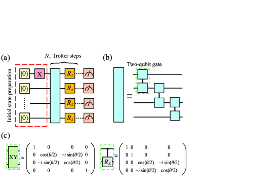
Figure 1: (Color online) (a) The schematic diagram of quantum circuit, which includes the initialization, $N_{T}$ Trotter steps, and measurements. The preparation for the initial state is in the red dashed box including a NOT gate (i.e. the X gate). The blue rectangle represents a layer of two-qubit gates. The orange rectangles represent single-qubit $R_{z}$ gates. (b) The schematic diagram of a layer of two-qubit gates. (c) The matrix representations for two types of 2-qubit gates: XY gates and controlled-$R_{x}$ gates.

2 Model

In this paper, we study the particle transport in the discrete-time evolution in the quantum transverse-field XY model. The purpose of this study is to investigate whether some typical quantum phenomena occurring in the continuous-time limit can be qualitatively observed in discrete-time evolution when the step size is large. The typical quantum phenomena we concerned here including resonant tunneling and localization effect, which caused by interference during the particle transport. Generally, the quantum transverse-field XY model can be used to describe the propagation of spin excitations, or particle transport when spin excitations can be treated as particles [46]. Additionally, in the quantum transverse-field XY model, the corresponding discrete-time evolution operator can be mapped into a quantum circuit according to the Trotter-Suzuki decomposition. Therefore, we investigate the particle transport with the quantum transverse-field XY model

$$H=\sum_{j}^{N-1}J_{j}H_{j,j+1}^{XY}+\sum_{j}^{N}V_{j}H_{j}^{Z},$$ (1)

where $j$ is the lattice site, $N$ is the system size, $J_{j}$ is the interaction strength and $V_{j}$ is the transverse-field strength. $H_{j,j+1}^{XY}=(\sigma_{j}^{x}\sigma_{j+1}^{x}+\sigma_{j}^{y}\sigma_{j+1}^{y})/4$ and $H_{j}^{Z}=\sigma_{j}^{z}/2$, where $\sigma_{j}^{i}$ $(i=x,y,z)$ represents the Pauli matrix at the $j$th site. In the case of $J_{j}<0$ and $V_{j}<0$, the ground state of the transverse-field XY chain is $\left|00...0\right\rangle$. In this work, we consider the time evolution of the initial state $\left|\psi(0)\right\rangle=\left|10...0\right\rangle$ which represents a spin excitation on the first site. The time evolution is in the subspace of single spin excitation.

The time evolution operator $U(t)$ of quantum transverse-field XY model can be approximated with a quantum circuit. According to Trotter-Suzuki decomposition, $U(t)$ can be expanded approximately

$$U(t)=e^{-iHt}\approx\left(\prod_{j=1}^{N-1}U_{j,j+1}^{XY}(J_{j}\tau)\prod_{j=1}^{N}U_{j}^{Z}(V_{j}\tau)\right)^{N_{T}},$$ (2)

where $N_{T}$ is the number of Trotter steps, $\tau=t/N_{T}$ is the size of each Trotter step. $U_{j,j+1}^{XY}(\theta_{j})=e^{-iH_{j,j+1}^{XY}\theta_{j}}$ and $U_{j}^{Z}\left(\phi_{j}\right)=e^{-iH_{j}^{Z}\phi_{j}}$, where $\theta_{j}=J_{j}\tau$ and $\phi_{j}=V_{j}\tau$.

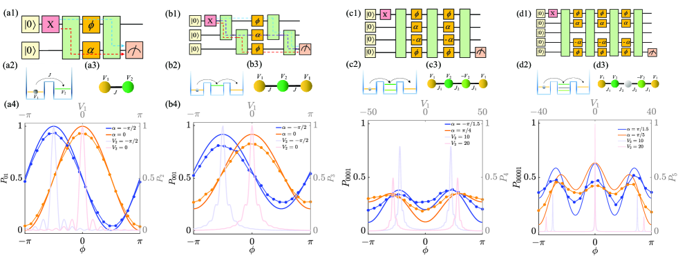
Figure 2: (Color online) (a1)-(d1) The circuit systems. The parameters of $R_{z}$ gates are marked on the orange squares. For convenience, in (c1) and (d1) we use single green rectangle to denote a layer of two-qubit gates. (a2)-(d2) The quantum wells. The energy levels of the wells are denoted by the horizontal lines in the wells. (a3)-(d3) The tight-binding chain. (a4)-(d4) Numerical result of the discrete-time evolution. The solid curves represent the probability of observing the spin excitation on the last qubit after the time evolution. The curves with circles are the results obtaining on a IBM quantum computer. The curves with light colors are the numerical result of the continuous-time evolution.

The corresponding discrete-time evolution is realized with the quantum circuit as shown in Fig. 1(a). The time evolution of each term, i.e. $U^{XY}$ and $U^{Z}$, are two-qubit XY gate and single-qubit $R_{z}$ gate, respectively. The circuit has $N$ qubits $\{q_{1},q_{2},...,q_{N}\}$ and $N_{T}$ Trotter steps, and every Trotter step contains one layer of two-qubit XY gates and one layer of single-qubit $R_{z}$ gates (We neglect $R_{z}$ gates in the last Trotter step, because these gates does not have any effect on the distribution of the spin excitation). In a quantum circuit, a NOT gate (i.e. the Pauli $\sigma_{x}$ matrix) can flip the qubit $\left|0\right\rangle$ to $\left|1\right\rangle$, therefore we prepare the initial state $\left|\psi(0)\right\rangle$ by applying a NOT gate on the first qubit, i.e. $\left|\psi(0)\right\rangle=\sigma_{1}^{x}\left|0\right\rangle^{N}=\left|10...0\right\rangle$ [see the dashed rectangle in Fig. 1(a)]. The matrix representation of XY gate is shown in Fig. 1(c).

The behavior of a spin excitation under discrete-time evolution depends on step size. When the Trotter step size is sufficiently small, the propagation of a spin excitation in quantum circuit is equivalent to the particle transport in continuous-time evolution. In this case, the propagation of spin excitation can exhibit some typical physical phenomena in particle transport. A natural question to ask is, in shallow quantum circuits with a large Trotter step size, whether some physical phenomena during continuous-time evolution nevertheless remains, so that we can observe these phenomena using fewer quantum gates. In the following text, we show that we observe the resonant tunneling and localization effect in shallow circuits even if the Trotter step size is large.

3 Resonant tunneling for large Trotter step size

In this section, we study the resonance phenomenon related to the transport of the spin excitation during the discrete-time evolution with a large step size. We study the situation where the size of the circuit system is $N=2,3,4,5$ respectively, where the spin excitation is created by a NOT gate and transmitted through the XY gate. In each one case, we qualitatively find the resonance tunneling in the limit of continuous-time evolution and give the corresponding minimum number of Trotter steps.

We also study the transport of a spin excitation through the controlled-$R_{x}$ gate. In quantum computing, computational errors occur due to the imperfect control and decoherence always error. The typical one is bit-flip error corresponding to an unwanted NOT gate. So studying the transmission of the spin excitation can help us understand the propagating of bit-flip errors. In actual quantum circuits, errors are not only transmitted, but also replicated. For example, a single-qubit error will become a multi-qubit error after passing through the controlled-$R_{x}$ gate. This effect potentially has a greater impact in quantum computing, because multi-qubit errors can lead to the failure of quantum error correction. So in this section, we also study the behavior of a spin excitation propagating through the controlled-$R_{x}$ gate and find the resonance phenomenon similar to that propagating through the XY gate.

3.1 Resonant tunneling in two-qubit circuit

We first discuss the case of $N=2$. The Hamiltonian of the transverse-field XY model with 2 sites is

$$H=J(\sigma_{1}^{x}\sigma_{2}^{x}+\sigma_{1}^{y}\sigma_{2}^{y})/4+V_{1}\sigma_{1}^{z}/2+V_{2}\sigma_{2}^{z}/2.$$ (3)

According to the Trotter-Suzuki decomposition, the time evolution operator can be approximated using a sequence of quantum gates

$$U(t)=e^{-iHt}\approx[U_{1,2}^{XY}(J\tau)U_{1}^{Z}(V_{1}\tau)U_{2}^{Z}(V_{2}\tau)]^{N_{T}},$$ (4)

where $U_{j,j+1}^{XY}(J_{j}\tau)=e^{-i(\sigma_{j}^{x}\sigma_{j+1}^{x}+\sigma_{j}^{y}\sigma_{j+1}^{y})J_{j}\tau}$, $U_{j}^{Z}\left(V_{j}\tau\right)=e^{-i\sigma_{1}^{z}V_{j}\tau/2}$, and $\tau=t/N_{T}$. The right side of ”$\approx$” in Eq. (4) represents the discrete-time evolution. The accuracy of the approximation increases with $N_{T}$. In Fig. 2(a1), we show the schematic diagram of the quantum circuit corresponding to discrete-time evolution when $N_{T}=2$ (the last two $R_{z}$ gates have been ignored, and so do the other systems). As we can see, the yellow squares represent that the qubits are initialized to $\left|00\right\rangle,$ which is the ground state of $H$ in the case of $V_{1},V_{2}<0$ and $J\ll V_{1}+V_{2}$. Following the initialization, a NOT gate on the first qubit flips $\left|00\right\rangle$ into $\left|10\right\rangle$, which represents that there is a spin excitation on the first qubit. $\left|10\right\rangle$ is the initial state that we want to prepare. Due to the symmetry of Hamiltonian, the spin excitation lies in the subspace spanned by {$\left|10\right\rangle$, $\left|01\right\rangle$}. In this single-spin-excitation subspace, we can regard a spin excitation as a particle moving in a $2$-site tight-binding chain [see Fig. 2(a3)], and the corresponding Hamiltonian is

$$H=J\left(\left|10\right\rangle\left\langle 01\right|+\left|01\right\rangle\left\langle 10\right|\right)+V_{1}\left|10\right\rangle\left\langle 10\right|+V_{2}\left|01\right\rangle\left\langle 01\right|,$$ (5)

where $\left|10\right\rangle$ or $\left|01\right\rangle$ represents a particle in the first or second site respectively, $J$ is the tunneling strength, $V_{1}$ and $V_{2}$ are the on-site potentials. In this chain system with fixed parameters $J$, $V_{2}$ and variable $V_{1}$, resonance phenomenon can be observed [47, 48, 49, 50, 51]: Assuming that a particle is on the first site at $t=0$, the probability, which is denoted by $P_{2}(V_{1},t)$, of observing the particle on the second site at any time $t$ reaches maximum when $V_{1}=V_{2}$. We numerically simulate this phenomenon in a discrete-time evolution with a large $N_{T}$ in Fig. 2(a4). We exhibit $P_{2}$ at $t=15$ (units of $1/J$, $J=0.1$) with the transparent lines for $V_{2}=0,-\pi/2$. As expected, $P_{2}$ has one resonance peak at $V_{1}=V_{2}$. We can understand this phenomenon more visually with the help of double-well system as shown in Fig. 2(a2). Supposing that a particle is bounded in the left well at the initial time, and then it will tunnel to the right well with a certain probability. When the potential energies on both sides are equivalent (i.e. $V_{1}=V_{2}$), the tunneling probability reaches maximization.

We wonder, when $N_{T}$ is small, whether we can qualitatively observe a similar resonant effect as the large $N_{T}$ limit. Motivated by this, we discuss the case of $N_{T}=2$. The parameters are redefined as $\theta=J\tau,\phi=V_{1}\tau,$ and $\alpha=V_{2}\tau$ for convenience. Our concern is the probability of finding spin excitation on the $2$nd qubit. Figure 2(a1) shows two propagation paths of the spin excitation from the $1$st to the $2$nd qubit. The blue path contributes $-i\sin\theta\cos\theta e^{i(\alpha-\phi)/2}$ to the amplitude, the purple path contributes $-i\sin\theta\cos\theta e^{-i(\alpha-\phi)/2}$ to the amplitude, so the final state of the quantum circuit reads

$$U_{1,2}^{XY}\left(\theta\right)U_{2}^{Z}\left(\alpha\right)U_{1}^{Z}\left(\phi\right)U_{1,2}^{XY}(\theta)\left|10\right\rangle=A_{10}\left|10\right\rangle+A_{01}\left|01\right\rangle,$$

where $A_{01}=-i\sin\theta\cos\theta(e^{-i(\alpha-\phi)/2}+e^{i(\alpha-\phi)/2})$. The probability of spin excitation measured on the second qubit is

$$P_{01}(\theta,\phi)=2\sin^{2}\theta\cos^{2}\theta\left(1+\cos(\alpha-\phi)\right).$$ (6)

In Fig. 2(a4), we plot $P_{01}$ as function of $\phi$ with $\theta=\pi/2$ and $\alpha=0,-\pi/2$. The accurate results (solid lines) computed using QuESTlink coincide with the experimental outcomes (solid lines with point symbols) computed using the IBM quantum device ”ibmq_rome”. The resonance peak is seen near $\phi=\alpha$, which is related to the interference term $2\sin^{2}\theta\cos^{2}\theta\cos(\alpha-\phi)$ in Eq. (6). $P_{2}$ coincides well with $P_{01}$, both of them have only one peak and the position of the peak is $\alpha=\phi$ (i.e. $V_{1}=V_{2}$). The above analysis indicates that only two Trotter steps are required for the circuit to exhibit resonant tunneling similar to the continuous-time evolution (i.e. $N_{T}$ is enough large).

3.2 Multi-qubit system

In this section we discuss the multi-qubit quantum circuits with the system sizes $N=3,4,5$ respectively.

We first discuss three-qubit system. The Hamiltonian of the transverse-field XY chain with $3$ sites reads

$$H = J\sum_{j}^{2}(\sigma_{j}^{x}\sigma_{j+1}^{x}+\sigma_{j}^{y}\sigma_{j+1}^{y})/4$$ (7)

$$+V_{1}\sigma_{1}^{z}/2+V_{2}\sigma_{2}^{z}/2+V_{1}\sigma_{3}^{z}/2.$$

The corresponding time evolution can be approximated,

$$U(t) = e^{-iHt}\approx[U_{1,2}^{XY}(J\tau)U_{2,3}^{XY}(J\tau)U_{1}^{Z}(V_{1}\tau)\times$$ (8)

$$U_{2}^{Z}(V_{2}\tau)U_{3}^{Z}(V_{1}\tau)]^{N_{T}},$$

where $U_{j,j+1}^{XY}(J_{j}\tau)=e^{-i(\sigma_{j}^{x}\sigma_{j+1}^{x}+\sigma_{j}^{y}\sigma_{j+1}^{y})J_{j}\tau}$, $U_{j}^{Z}\left(V_{j}\tau\right)=e^{-i\sigma_{1}^{z}V_{j}\tau/2}$, $\tau=t/N_{T}$. The right side of above equation represents the discrete-time evolution. The quantum circuit implementing the discrete-time evolution is shown in Fig. 2(b1). We concern the time evolution of single spin excitation. When the single spin excitation can be treated as a particle, the transverse-field XY chain is equal to a $3$-site tight-binding chain [see Fig. 2(b3)],

$$H = J\left(\left|100\right\rangle\left\langle 010\right|+\left|010\right\rangle\left\langle 100\right|+\mathrm{h.c.}\right)+V_{1}\left|100\right\rangle\left\langle 100\right|$$ (9)

$$+V_{2}\left|010\right\rangle\left\langle 010\right|+V_{1}\left|001\right\rangle\left\langle 001\right|.$$

where $J$ is the coupling strength, the potentials on three sites are $V_{1},V_{2}$ and $V_{1}$ respectively. In the case that $V_{1}$ is the only variable parameter, the resonance phenomenon means that the probability, $P_{3}(t,V_{1})$, of finding particle on the $3$th site reaches maximum at $V_{1}=V_{2}$. We numerically simulate the discrete-time evolution with a large $N_{T}$ and show the resonance phenomenon. The initial state is $\left|100\right\rangle$. In Fig. 2(b4), we plot $P_{3}$ as the function of $V_{1}$ at $t=22$ (units of $1/J$, $J=0.1$) with the transparent lines. $P_{3}$ has one resonance peak at $V_{1}=V_{2}$. Similarly, we can consider the resonance phenomenon with a triple-well system [see Fig. 2(b2)], whose Hamiltonian can be written as Eq. (9). In the triple-well system, the probability of the particle tunneling from the left well to the right well reaches maximization at $V_{1}=V_{2},$ when the resonance occurs.

As for the small $N_{T}$, we find that only two Trotter steps are required for the $3$-qubit circuit to exhibit resonant tunneling. The parameters of the $3$-qubit circuit are redefined as $J\tau=\theta,V_{1}\tau=\phi,V_{2}\tau=\alpha$. As shown the blue, red and purple dashed lines in Fig. 2(b1), the spin excitation goes through three paths. The blue and red paths contribute $\cos\theta(-i\sin\theta)(-i\sin\theta)e^{-i\alpha/2}$ to the amplitude, and the purple path contributes $-i\sin\theta\cos\theta e^{i\left(\alpha/2-\phi\right)}\cos\theta(-i\sin\theta)$ to the amplitude. The amplitude of the final state on the third qubit is

$$A_{001}=-\sin^{2}\theta\cos\theta\left(2e^{-i\alpha/2}+\cos\theta e^{i\left(\alpha/2-\phi\right)}\right).$$ (10)

Accordingly, the probability of finding the spin excitation on the $3$rd qubit is

$$P_{001}(\theta,\phi)=\sin^{4}\theta\cos^{2}\theta(4+\cos^{2}\theta+4\cos\theta\cos\left(\alpha-\phi\right)).$$ (11)

The interference term $4\sin^{4}\theta\cos^{3}\theta\cos\left(\alpha-\phi\right)$ dominates the resonant tunneling effect. In Fig. 2(b4), we plot $P_{001}$ as function of $\phi$ with $\theta=\pi/2$ and $\alpha=0,-\pi/2$. The accurate results (solid lines) computed using QuESTlink coincide with the experimental outcomes (solid lines with point symbols) computed using the IBM quantum device ”ibmq_rome”. As we can see, $P_{3}$ coincides well with $P_{001}$, both of them have only one peak and the position of the peak is $\alpha=\phi$ (i.e. $V_{1}=V_{2}$). The above analysis indicates that only two Trotter steps are required for the $3$-qubit circuit to exhibit similar resonant tunneling in the continuous-time limit.

We also study the four-qubit system. The Hamiltonian of the $4$-site transverse-field XY chain we studied is

$$H = J_{1}\sum_{j=1,3}(\sigma_{j}^{x}\sigma_{j+1}^{x}+\sigma_{j}^{y}\sigma_{j+1}^{y})/4+J_{2}(\sigma_{2}^{x}\sigma_{3}^{x}+\sigma_{2}^{y}\sigma_{3}^{y})/4$$ (12)

$$+V_{1}\sigma_{1}^{z}/2+V_{2}\sigma_{2}^{z}/2-V_{2}\sigma_{3}^{z}/2+V_{1}\sigma_{4}^{z}/2.$$

The corresponding discrete-time evolution is in the form

$$U(t) = e^{-iHt}\approx[U_{1,2}^{XY}(J_{1}\tau)U_{2,3}^{XY}(J_{2}\tau)U_{3,4}^{XY}(J_{1}\tau)\times$$ (13)

$$U_{1}^{Z}(V_{1}\tau)U_{2}^{Z}(V_{2}\tau)U_{3}^{Z}(-V_{2}\tau)U_{3}^{Z}(V_{1}\tau)]^{N_{T}},$$

where $U_{j,j+1}^{XY}(J_{j}\tau)=e^{-i(\sigma_{j}^{x}\sigma_{j+1}^{x}+\sigma_{j}^{y}\sigma_{j+1}^{y})J_{j}\tau}$, $U_{j}^{Z}\left(V_{j}\tau\right)=e^{-i\sigma_{1}^{z}V_{j}\tau/2}$, $\tau=t/N_{T}$. We plot the quantum circuit implementing the discrete-time evolution in Fig. 2(c1). In the single-particle subspace, the equivalent $4$-site tight-binding chain is

$$H = J_{1}\left(\left|1000\right\rangle\left\langle 0100\right|+\left|0010\right\rangle\left\langle 0001\right|\right)+J_{2}(\left|0100\right\rangle\left\langle 0010\right|$$ (14)

$$+\left|0010\right\rangle\left\langle 0100\right|)+V_{1}\left|1000\right\rangle\left\langle 1000\right|+V_{2}\left|0100\right\rangle\left\langle 0100\right|$$

$$-V_{2}\left|0010\right\rangle\left\langle 0010\right|+V_{1}\left|0001\right\rangle\left\langle 0001\right|.$$

As we marked in Fig. 2(c4), the coupling strengths between neighboring sites are $J_{1},J_{2}$, and $J_{1}$ respectively, and the on-site potentials on the four sites are $V_{1},V_{2},-V_{2},V_{1}$ respectively. In the condition of $J_{1}\ll J_{2},V_{2}$, we numerically simulate the discrete-time evolution of one particle with a large $N_{T}$. In Fig. 2(c4), $P_{4}(V_{1},t)$, which is the probability of finding the particle on the $4$th site, is plotted as function of $V_{1}$ with the transparent lines. The cases of $V_{2}=10$ and $V_{2}=20$ are studied when $J_{1}=1$, $t=3$ (units of $1/J_{1}$), $J_{2}=20$. As we can see, the resonant peaks can be observed near $\sqrt{J_{2}^{2}+V_{2}^{2}}$ and $-\sqrt{J_{2}^{2}+V_{2}^{2}}$, and the distance between the resonance peaks varies when $V_{2},-V_{2}$ change. One can observe the same resonance phenomenon in a triple-well system [see Fig. 2(c2)]. The energy levels of the left and right wells are $V_{1}$, the middle well has two energy levels: $\sqrt{J_{2}^{2}+V_{2}^{2}}$ and $-\sqrt{J_{2}^{2}+V_{2}^{2}}$. If there is a particle in the left well at the initial moment, then we can detect this particle in the right well with a certain probability. When $V_{1}$ is close to $\sqrt{J_{2}^{2}+V_{2}^{2}}$ or $-\sqrt{J_{2}^{2}+V_{2}^{2}}$, the probability of finding particle in right well reaches the maximum. The distance of the two peaks varies with $V_{2}$.

When $N_{T}$ is small, we find that only three Trotter steps are required for the $4$-qubit circuit to qualitatively exhibit resonant tunneling. We investigate the propagation of the spin excitation in the circuit. $P_{0001}$, which is the probability of finding spin excitation on the $4$th qubit, is shown (the solid lines) in Fig. 2(c1). The parameters are redefined as $J_{1}\tau=\theta_{1},J_{2}\tau=\theta_{2},V_{1}\tau=\phi,V_{2}\tau=\alpha$. With $\theta_{1}=\theta_{2}=\pi/1.5$, we plot two cases of $\alpha=\pi/4$ and $\alpha=-\pi/1.5$. Compare Fig. 2(c4) with (a4) or (b4), we find that the peaks are not at $\alpha$ and $-\alpha$. However, the distance between every two peaks is changed when $\alpha$ is adjusted, which is the major characteristic of the resonant tunneling effect.

Finally, we discuss the five-qubit system. The Hamiltonian of the $5$-site transverse field XY chain we studied is

$$H = J_{1}\sum_{j=1,4}(\sigma_{j}^{x}\sigma_{j+1}^{x}+\sigma_{j}^{y}\sigma_{j+1}^{y})/4$$ (15)

$$+J_{2}\sum_{j=2,3}(\sigma_{j}^{x}\sigma_{j+1}^{x}+\sigma_{j}^{y}\sigma_{j+1}^{y})/4$$

$$+V_{1}\sigma_{1}^{z}/2+V_{2}\sigma_{2}^{z}/2-V_{2}\sigma_{4}^{z}/2+V_{1}\sigma_{5}^{z}/2.$$

The quantum circuit implementing the discrete-time evolution is shown in Fig. 2(d1). In the single-particle subspace, the equivalent $5$-site tight-binding chain is

$$H = [J_{1}\left(\left|10000\right\rangle\left\langle 01000\right|+\left|00010\right\rangle\left\langle 00001\right|\right)$$

$$+J_{2}(\left|01000\right\rangle\left\langle 00100\right|+\left|00100\right\rangle\left\langle 00010\right|)+\mathrm{h.c.}]$$

$$+V_{1}\left|10000\right\rangle\left\langle 10000\right|+V_{2}\left|01000\right\rangle\left\langle 01000\right|$$

$$-V_{2}\left|00010\right\rangle\left\langle 00010\right|+V_{1}\left|00001\right\rangle\left\langle 0001\right|.$$

The schematic diagram of Hamiltonian Eq. (3.2) is shown in Fig. 2(c4). We numerically simulate the continuous-time evolution (implemented with the large $N_{T}$). The system parameters are $J_{1}=0.1$, $t=40$ (units of $1/J_{1}$), $J_{2}=20$, $V_{2}=10,20$. We focus on the probability $P_{5}(V_{1},t)$ (see the transparent lines in Fig. 2(d4)) of finding particle on the $5$th site. As we can see, $P_{5}(V_{1},t)$ will reach the maximum when $V_{1}\approx 0,\pm\sqrt{2J_{2}^{2}+V_{2}^{2}}$, and the distance of the peaks is affected by $V_{2}$. The same resonance phenomenon can be observed in a triple-well system (see Fig. 2(d2)). The energy levels on the left and right wells are $V_{1}$, the middle well has three energy levels: $\sqrt{2J_{2}^{2}+V_{2}^{2}}$, $0$, and $-\sqrt{2J_{2}^{2}+V_{2}^{2}}$. When $V_{1}=\sqrt{J_{2}^{2}+V_{2}^{2}}$, $0$, or $-\sqrt{J_{2}^{2}+V_{2}^{2}}$, the probability of finding particles in right well reaches the maximum. The distances between three peaks vary with $V_{2}$.

When $N_{T}$ is small, we find that only four Trotter steps are required for the circuit to qualitatively exhibit resonant tunneling. We investigate the propagation of the spin excitation in the circuit shown in Fig. 2(d1). We redefine parameters as $J_{1}\tau=\theta_{1},J_{2}\tau=\theta_{2},V_{1}\tau=\phi,V_{2}\tau=\alpha,$ and denote the probability of finding spin excitation on the $5$th qubit as $P_{00001}$. Figure 2(d4) exhibits $P_{00001}$ (the solid lines) as function of $\phi$ by fixing $\alpha,\theta_{1}=\pi/3$ and $\theta_{2}=\pi/1.2$. We compare two cases that $\alpha$ is $\pi/1.5,\pi/5$ respectively. The distance between the peaks is changed when $\alpha$ is adjusted, which is the major characteristic of the resonant tunneling effect.

3.3 CR model

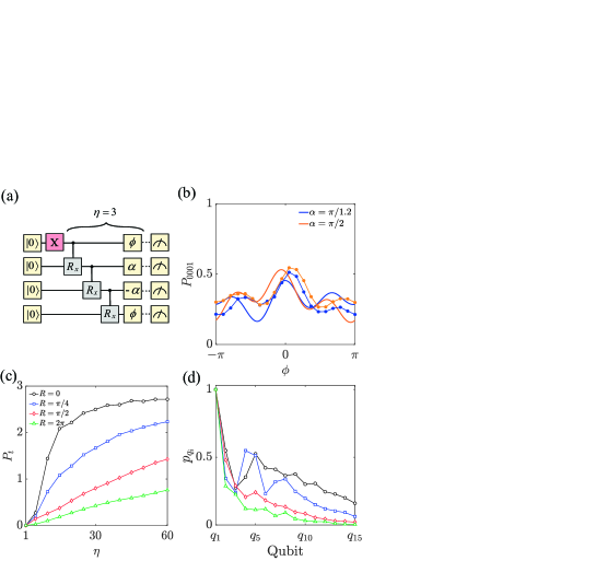
Figure 3: (Color online) (a) 4-qubit circuit. The two-qubit XY gates are replaced by controlled-$R_{x}$ gates. (b) The probability of finding the spin excitation on the last qubit as function of $\phi$. (c) The probability of observing the spin excitation on the last third of the qubits varies with Trotter step $\eta$. (d) The probability distribution of spin excitation at $\eta=10$. (c) and (d) use the same legend and drawing parameter $\theta=\phi=\pi/2$.

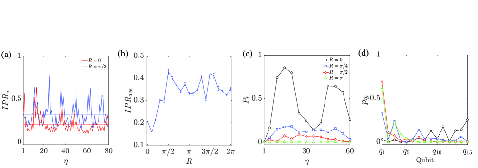
Figure 4: (Color online) (a) The IPR_η varies with Trotter number $\eta$, the drawing parameters are $N=15,N_{T}=80,\theta=\phi=\pi/2$. The red and blue lines represent the ordered and disordered case respectively. The horizontal lines are the average value of IPR_η, i.e. IPR_ave. (b) IPR_ave as function of the degree of randomness. For a fixed $R$, we have $20$ data. The blue line is the average value of the $20$ data, and error bar is the variance. (c) The physical quantity $P_{t}$ is plotted in disordered configuration. (d) The probability distribution of spin excitation when $\eta=10$. (c) and (d) share the same legend.

In this section, the propagation of the spin excitation through controlled-$R_{x}$ gates is investigated. In the previous section, the spin excitation is created by a NOT gate and propagated through the XY gate. Here, we study the behavior of the spin excitation propagating through the controlled-$R_{x}$ gates. The controlled-$R_{x}$ gate is expressed as

$$U^{CR_{x}}=\left|0\right\rangle\left\langle 0\right|\otimes I+\left|1\right\rangle\left\langle 1\right|\otimes e^{-i\theta\sigma_{x}/2},$$ (17)

the matrix representation of $U^{CR_{x}}$ is shown in Fig. 1(c). Consider the situation that a spin excitation on the first qubit passes through a controlled-$R_{x}$ gate, we get the following equation

$$U^{CR_{x}}\left|10\right\rangle=\cos\frac{\theta}{2}\left|10\right\rangle-i\sin\frac{\theta}{2}\left|11\right\rangle.$$ (18)

The above equation indicates that after passing through a controlled-$R_{x}$ gate, the spin excitation becomes a two-qubit entangled state. From the view point of propagation of the bit-flip error, this indicates that the controlled-$R_{x}$ gate can transform a single-qubit error to a multi-qubit error. We take the four-qubit circuit in Fig. 3(a) as a example to study the behavior of spin excitation propagating through controlled-$R_{x}$ gates under the discrete-time evolution with a large step size. We observed the probability of finding the spin excitation on the $4$th qubit and denote the probability as $P_{0001}$. In Fig. 3(b), $P_{0001}$ shows two resonant peaks, the distance between the two resonant peaks is changed as the $\phi$ varies. This indicates that even if the spin excitations are propagated by the controlled-$R_{x}$ gate, when the step size is large we can qualitatively observe the resonance phenomenon that occurs in the continuous-time limit.

4 Localization for large Trotter step size

In this section, we study whether the localization can be observed in the discrete-time evolution when the Trotter step size is large. We still study the transverse field XY model, but the parameters of a layer of $U^{Z}$ (i.e. a layer of single-qubit $R_{z}$ gates) are random. We compare the probability distribution of the spin excitation in different configurations of the parameters of a layer of $R_{z}$ gates. The stronger the randomness of the parameters, the higher the localization of the distribution of the spin excitation, which means higher the probability of observing the spin excitation near a specific qubit. In this study, the propagation of the bit-flip error (i.e. an unwanted NOT gate) is similar to the transport of the spin excitation. Therefore, the localization indicates that the bit-flip error may be localized near a specific qubit and may not affect the measurement on distant qubits.

The localization phenomenon is studied[52, 53, 54, 55, 56] during the discrete-time evolution with a large step size. We begin with the Hamiltonian in Eq. (1) with $J_{j}=J$. For convenience the parameters are defined as $J\tau=\theta,V_{j}\tau=\phi_{j}.$ For the purpose of investigating localization, one layer of parameters for $U^{Z}$ in Eq. (2) is {$\phi_{j}$}$\equiv${$\phi_{1},-\phi_{2},\phi_{3},-\phi_{4},\cdots$}, where $\phi_{j}=\phi+r_{j}$, $r_{j}\in[-R$, $R]$ is a random number. {$\phi_{j}$} is the same for each layer of $U^{Z}$. {$\phi_{j}$} is ordered (periodic) configuration when $R=0$ and disordered configuration when $R>0$. The inverse participation ratio [57] (IPR) is a measure of localization and defined as

$$IPR_{\eta}=\sum_{i=1}^{N}|P_{i}(\eta)|^{4},$$ (19)

where

$$P_{i}(\eta) = \left\langle i\right.\left|\psi(\eta)\right\rangle,$$

$$\left|\psi(\eta)\right\rangle = (\prod_{j=1}^{N-1}U_{j,j+1}^{XY}(\theta_{j})\prod_{j=1}^{N}U_{j}^{Z}(\phi_{j}))^{\eta}\left|\psi(0)\right\rangle.$$ (20)

$\left|\psi(\eta)\right\rangle$ represents the quantum state at the $\eta$th Trotter step, $P_{i}(\eta)$ represents the corresponding amplitude at the $i$th qubit. In general, IPR_η varies from $1/N$ (system size) to $1$ and a large value of IPR_η means a stronger localization effect. The localization of $\left|\psi(\eta)\right\rangle$ changes with $\eta$, thus the average IPR is introduced to character the average level of localization during the whole discrete-time evolution[42],

$$IPR_{ave}=\frac{1}{N_{T}}\sum_{\eta=1}^{N_{T}}IPR_{\eta}.$$ (21)

In Fig. 4(a), we plot $IPR_{\eta}$ (the solid lines) as function of $\eta$ for the ordered ($R=0$) and disordered ($R=\pi/2$) configuration respectively. The drawing parameters are $N=N_{T}=80,\theta=\phi=\pi/2$. $IPR_{\eta}$ for both the ordered (the red lines) and disordered (the red lines) configuration show a periodic-like behavior and is larger than $1/N$, which means $\left|\psi(\eta)\right\rangle$ exhibits localization effect in both cases. However, the average value (the horizontal line), i.e. $IPR_{ave}$, of the blue line is larger than the red line, and the peaks of the blue line are closer to $1$. This indicates stronger localization in the disordered case. Furthermore, in Fig. 4(b), we show the $IPR_{ave}$ varying with the degree $R$ of the randomness. With the increase of disorder, the localization becomes stronger.

In this study, the propagation of the bit-flip error (i.e. an unwanted NOT gate) is similar to the transport of the spin excitation, thus the localization implies that single bit-flip error propagated by disordered {$U_{j}^{Z}(\phi_{j})$} does not affect the measurement on a distant qubit. To illustrate this point, we propose a physical quantity $P_{\mathrm{t}}\equiv\sum_{q_{i}=2N/3}^{N}p_{q_{i}}$ which is the average probability of finding the spin excitation on the last third of the qubits, where $p_{q_{i}}$ denotes the probability of finding the error on the $i$th qubit. The smaller the $P_{\mathrm{t}}$, the shorter the distance the spin excitation travels. As shown in Fig. 4(c), $P_{\mathrm{t}}$ is lower when $r_{i}\neq 0$, which demonstrates that only a little probability is propagated to the last several qubits. $P_{\mathrm{t}}$ is almost vanishing as the degree of randomness keeps increasing. In Fig 4(d), we plot $p_{q_{i}}$ at $\eta=10$. As we can see, more probabilities are propagated to the last few qubits for $r_{i}=0$ and are localized at the first few qubits for $r_{i}\neq 0$. Figure 4(d) also show that the greater the degree of randomness, the stronger the localization phenomenon. Above results indicates that the measurement is almost unaffected by the bit-flip error on the first qubit for $r_{i}\neq 0$.

The above conclusion still holds if XY gates in the circuit are replaced by controlled-$R_{x}$. As shown in Fig. 3(c), $P_{t}$ grows with the increasing Trotter steps. However, $P_{\mathrm{t}}$ becomes lower when the random perturbation is applied to a layer of $R_{z}$ gates, which means less probabilities are propagated to the end of the circuit. With the increasing degree of disorder, the inhibiting effect is more significant. In Fig. 3(d), we plot the probability distribution of spin excitation when $\eta=10,\theta=\phi=\pi/2$. These results show that, with a strong randomness of {$\phi_{j}$}, the spin excitation will not be propagated to the farther qubits. At the same time, this also shows that the randomness of the parameters will inhibit the propagation of the bit-flip error and protect the measurement on the distant qubits is not affected.

5 Conclusions

We study the transport of the spin excitation in the discrete-time evolution using Trotter circuits with a large step size, and qualitatively observe the quantum phenomena in the continuous-time limit, i.e. the resonant tunneling and localization. We observe the resonance phenomenon during the transport of the spin excitation in systems of sizes $N=2,3,4,5$ respectively. The probability distribution of spin excitations propagating through several Trotter steps agree qualitatively with that in the continuous-time limit. The corresponding minimum number of Trotter steps is given for each system size. In a Trotter circuit with random parameters of $R_{z}$ gates, we can observe the localization phenomenon of the spin excitation distribution even with a large step size. We study the spin excitation propagating through the XY gates and also through the controlled-$R_{x}$ gates. Our research indicates that a discrete-time quantum simulator with a large step size can qualitatively demonstrate some physical phenomena in the continuous-time limit. Qualitative observations require fewer quantum gates than quantitative calculations and therefore are a promising application on near-term quantum computers. In quantum computing, some errors, such as bit-flip errors, behave like spin excitations, thus, our finding can be used to understand the propagating of these errors in the quantum circuits.

References

References

- [1] R. P. Feynman, Simulating physics with computers, Int J Theor Phys 21, 467–488 (1982)
- [2] M. A. Nielsen and I. L. Chuang, Quantum Computation and Quantum Information, Cambridge University Press, Cambridge, (2010)
- [3] F. Arute et al., Quantum supremacy using a programmable superconducting processor, Nature 574, 505 (2019)
- [4] S. Lloyd, Universal quantum simulators, Science 273, 1073 (1996)
- [5] A. M. Childs, D. Maslov, Y. Nam, N. J. Ross, and Y. Su, Toward the first quantum simulation with quantum speedup, Proceedings of the National Academy of Sciences 115, 9456 (2018)
- [6] A. M. Childs, Y. Su, M. C. Tran, N. Wiebe, and S. Zhu, Theory of trotter error with commutator scaling, Phys. Rev. X 11, 011020 (2021)
- [7] C. Yi, Robustness of discretization in digital adiabatic simulation, arXiv:2107.06404 (2021)
- [8] J. Preskill, Quantum computing in the NISQ era and beyond, Quantum 2, 79 (2018)
- [9] R. Landauer, Is quantum mechanics useful? Phil. Tran. R. Soc. Lond. 353, 367 (1995); R. Landauer, The physical nature of information, Phys. Lett. A 217, 188 (1996)
- [10] W. G. Unruh, Maintaining coherence in quantum computers, Phys. Rev. A 51, 992 (1995)
- [11] S. Haroche and J. M. Raimond, Quantum computing: dream or nightmare? Phys. Today 49, 51 (1996)
- [12] P. W. Shor, Scheme for reducing decoherence in quantum computer memory. Phys. Rev. A 52, R2493 (1995)
- [13] A. M. Steane, Error Correcting Codes in Quantum Theory. Phys. Rev. Lett. 77, 793 (1996)
- [14] A. R. Calderbank and P. W. Shor, Good Quantum Error Correcting codes exist, Phys. Rev. A 54, 1098 (1996)
- [15] R. Laamme, C. Miquel, J. P. Paz, and W. H. Zurek, Perfect Quantum Error Correcting Code. Phys. Rev. Lett. 77, 198 (1996)
- [16] C. H. Bennett, D. P. DiVincenzo J. A. Smolin, and W. K. Wooters, Mixed State Entanglement and Quantum Error Correction, Phys. Rev. A 54, 3824, (1996)
- [17] A. M. Steane, Multiple particle interference and quantum error correction, Proc. Royal Society of London A 452, 2551 (1996)
- [18] A. M. Steane, Simple quantum error correcting codes, Phys. Rev. A 54, 4741 (1996)
- [19] E. Knill and R. Laamme, A Theory of Quantum Error Correcting Codes. Phys. Rev. Lett. 84, 2525 (2000)
- [20] P. W. Shor, Fault-Tolerant quantum computation, Proc. 37th IEEE Symp. on Foundations of Computer Science, 56-65 (1996)
- [21] D. Gottesman, Fault-Tolerant Quantum Computation with Local Gates, J. Mod. Opt 47, 333 (2000)
- [22] E. Knill, R. Laamme, and W. H. Zurek, Accuracy threshold for Quantum Computation (1996)
- [23] A. Holmes, M. R. Jokar, G. Pasandi, Y. Ding, M. Pedram, and F. T. Chong, Nisq+: Boosting quantum computing power by approximating quantum error correction, arXiv:2004.04794 (2020)
- [24] Y. Ueno, M. Kondo, M. Tanaka, Y. Suzuki, and Y. Tabuchi, Qecool: On-line quantum error correction with a superconducting decoder for surface code, arXiv:2103.07526 (2021)
- [25] P. Das, A. Locharla, and C. Jones, Lilliput: A lightweight low-latency lookup-table based decoder for near-term quantum error correction, arXiv:2108.06569 (2021)
- [26] Y. Li and S. Benjamin, Practical Quantum Error Mitigation for Near-Future Applications, Phys. Rev. X 8, 031027 (2018)
- [27] S. Endo, Z. Cai, S. C. Benjamin, and X. Yuan, Hybrid quantum-classical algorithms and quantum error mitigation, J. Phys. Soc. Jpn 90. 032001 (2021)
- [28] A. Kandala, K. Temme, A. D. Córcoles, A. Mezzacapo, J. M. Chow, and J. M. Gambetta, Error mitigation extends the computational reach of a noisy quantum processor, Nature 567, 209–212 (2019)
- [29] J. J. Wallman and J. Emerson, Randomized compiling with twirling gates, Phys. Rev. A 94, 052325 (2016)
- [30] A. Strikis, D. Y. Qin, Y. Z. Chen, S. C. Benjamin, and Y. Li, Learning-based quantum error mitigation, PRX Quantum 2, 040330 (2021)
- [31] Z. Wang , Y. Z. Chen , Z. X. Song, D. Qin, H. K. Li, Q. J. Guo, H. Wang, C. Song, and Ying Li, Scalable evaluation of quantum-circuit error loss using Clifford sampling, Phys. Rev. Lett. 126, 080501 (2021)
- [32] V. N. Premakumar and R. Joynt, Error mitigation in quantum computers subject to spatially correlated noise, arXiv:1812.07076 (2018)
- [33] K. Temme, S. Bravyi, and J. M. Gambetta, Error mitigation for short-depth quantum circuits, Phys. Rev. Lett. 119, 180509 (2017)
- [34] C. Song, J. Cui, H. Wang, J. Hao, H. Feng, and Ying Li, Quantum computation with universal error mitigation on a superconducting quantum processor, Sci. Adv 5, eaaw5686 (2019)
- [35] A. Kandala, K. Temme, A. D. C orcoles, A. Mezzacapo, J. M. Chow, and J. M. Gambetta, Error mitigation extends the computational reach of a noisy quantum processor, Nature 567, 491-495 (2019)
- [36] M. Otten and S. K. Gray, Recovering noise-free quantum observables, Phys. Rev. A 99, 012338 (2019)
- [37] A. Tranter, P. J. Love, F. Mintert, N. Wiebe, and P. V. Coveney, Ordering of Trotterization: Impact on Errors in Quantum Simulation of Electronic Structure, Entropy 21, 1218 (2019)
- [38] C. Yi, Success of digital adiabatic simulation with large Trotter step, Phys. Rev. A 104, 052603 (2021)
- [39] P. J. J. O’Malley et al., Scalable Quantum Simulation of Molecular Energies, Phys. Rev. X 6, 031007 (2016)
- [40] A. M. Childs, Y. Su, M. C. Tran, N. Wiebe, and S. Zhu, Theory of Trotter Error with Commutator Scaling, Phys. Rev. X 11, 011020 (2021)
- [41] D. Poulin, M. B. Hastings, D. Wecker, N. Wiebe, A. C. Doherty, and M. Troyer, The trotter step size required for accurate quantum simulation of quantum Chemistry, Quantum Information & Computation 15, 361 (2015)
- [42] M. Heyl, P. Hauke, P. Zoller, Quantum localization bounds Trotter errors in digital quantum simulation, Sci Adv 5, eaau8342 (2019)
- [43] L. M. Sieberer, T. Olsacher, A. Elben, M. Hey, P. Hauke, F. Haake and P. Zoller, Digital quantum simulation, Trotter errors, and quantum chaos of the kicked top, NPJ quantum iniformation 5, 1-11 (2019)
- [44] J. T. Edwards and D. J. Thouless, Numerical studies of localization in disordered systems, J. Phys. C: Solid State Phys. 5 807 (1972)
- [45] M. Segev, Y. Silberberg, and D. N. Christodoulides, Anderson localization of light, Nature Photon 7, 197–204 (2013)
- [46] P. Jordan and E. Wigner, Über das Paulische Äquivalenzverbot, Z. Phys. 47, 631 (1928)
- [47] J. G. Wang, S. J. Yang, Ultracold bosons in a one-dimensional optical lattice chain: Newton’s cradle and Bose enhancement effect, Phys. Lett. A 381, 1665 (2017)
- [48] A. S. Buyskikh , L. Tagliacozzo, D. Schuricht, C. A. Hooley, D. Pekker, and A. J. Daley, Resonant two-site tunneling dynamics of bosons in a tilted optical superlattice, Phys. Rev. A 100, 023627 (2019)
- [49] S. Scherg, T. Kohlert, P. Sala, F. Pollmann, B. H. Madhusudhana, I. Bloch, and M. Aidelsburger, Observing non-ergodicity due to kinetic constraints in tilted Fermi-Hubbard chains, Nat. Commun 12, 4490 (2021)
- [50] R. Tsu and L. Esaki, Tunneling in a finite superlattice, Appl. Phys. Lett. 22, 562 (1973)
- [51] T. C. L. G. Sollner, W. D. Goodhue, P. E. Tannenwald, C. D. Parker, and D. D. Peck, Resonant tunneling through quantum wells at frequencies up to 2.5 THz, Appl. Phys. Lett. 43, 588 (1983)
- [52] P. W. Anderson, Absence of Diffusion in Certain Random Lattices, Phys. Rev. 109, 1492 (1957)
- [53] D. S. Wiersma, P. Bartolini, A. Lagendijk, and R. Righini, Localization of light in a disordered medium, Nature 390, 671–673 (1997)
- [54] B. L. Altshuler, D. Khmel’nitzkii, A. I. Larkin, and P. A. Lee, Magnetoresistance and Hall effect in a disordered two-dimensional electron gas, Phys. Rev. B 22, 5142 (1980)
- [55] D. Vollhardt, P. Wölfle, Scaling Equations from a Self-Consistent Theory of Anderson Localization, Phys. Rev. Lett. 48, 699 (1982)
- [56] A. N. Poddubny, M. V. Rybin, M. F. Limonov, and Y. S. Kivshar, Fano interference governs wave transport in disordered systems, Nat. Commun 3, 914 (2012)
- [57] F. Haake, Quantum Signatures of Chaos (Springer, 2010)