Analytical Galerkin boundary integrals of Laplace kernel layer potentials in $\mathbb{R}^{3}$

Abstract

A method for analytical computation of the double surface integrals for all layer potential kernels associated with the Laplace Green’s function, in the Galerkin boundary element method (BEM) in $\mathbb{R}^{3}$ using piecewise constant flat elements is presented. The method uses recursive dimensionality reduction from 4D ($\mathbb{R}^{2}\times\mathbb{R}^{2}$) based on Gauss’ divergence theorem. Computable analytical expressions for all cases of relative location of the source and receiver triangles are covered for the single and double layer potentials and their gradients with analytical treatment of the singular cases are presented. A trick that enables reduction of the case of gradient of the single layer to the same integrals as for the single layer is introduced using symmetry properties. The method was confirmed using analytical benchmark cases, comparisons with error-controlled computations of regular multidimensional integrals, and a convergence study for singular cases.

65R20, 65N30, 65N38

1 Introduction

The Galerkin BEM is a commonly used variant of general method of moments (MoM), where the basis and test functions are the same [7], and is often preferred as it yields symmetric matrices. A challenge with the method is efficient and accurate evaluation of double surface ($\mathbb{R}^{2}\times\mathbb{R}^{2}$) integrals. When the source and receiver triangles are well separated (regular integrals) efficient numerical procedures using exact analytical expressions for the potentials over the source triangles [8, 19, 5] and Gaussian quadrature over the receiver triangle can be employed. Moreover, the Galerkin integrals can be computed using multipole expansions [1, 6]. When the triangles have one or more common points all integrals are singular, and treated using special methods (e.g., [1, 2]). With two common vertices between source and receiver triangles the integrals are hypersingular and do not exist even in the Cauchy principal value sense, and requires a special treatment [19, 4, 15]. Depending on triangle proximity we also have the case of nearly singular integrals.

While the literature provides numerical methods for the Galerkin integrals, full analytical expressions were derived and analyzed only recently. Previously analytical results were only available for the self-action Galerkin integrals [3, 20]. The “modern” history of analytical expressions for the Galerkin integrals probably starts with [16], who used Gauss’ divergence theorem to reduce the volume integrals to surface integrals for homogeneous functions and introduced the concept of the primitive boundary function (PBF), though not in the context of the Galerkin method. The PBF is the integrand of the boundary integral that is related to the original integrand of the volume integral.

Lenoir [11] realized then that the PBF can be computed recursively for $d=4,3,2,1$ to reduce the 4D integrals for the single layer potential to a final form, which contains only elementary functions. This was restricted to the case when the planes of the source and receiver triangles are not parallel. Next Lenoir and Salles [12] considered the special case when source and receiver triangles are located in the same plane or parallel planes. The gradient of single layer is calculated for this special case. The same authors combined these two results and added the case of linear basis functions in [13, 18]. In [21] the expressions were further simplified and the number of cases needed to be considered reduced. An expression for the hypersingular integral was also presented, though no treatment of the singularity was provided. A related recent study is [14], where the focus is on single and double layer integrals. Analytical expressions for the double layer were obtained only when the source and receiver triangles have a common vertex or edge.

In comparison to previous work, we follow an independent approach to recursive dimensionality reduction, and a different triangle parametrization and treatment of the integrand. In our work this appears generally as a 4-parametric non-homogeneous function with 5 three dimensional vector coefficients. Homogenization of the PBF occurs via projections which can be efficiently generally handled using Gram-Schmidt orthogonalization. Further, we provide explicit expressions for the PBF in all dimensions and we found substantial simplifications related to the interplay of the 3D real space and 4D space in which integration occurs. We consider all cases of relative locations of the source and receiver triangles, and all layer potentials - including single and double layer potentials, the gradient of single layer potential, and the hypersingular case with analytical treatment of the singularity. This provides analytical expressions for the cases which were not considered before. We were able to reduce the gradient of the single layer to the same integrals as for the single layer using symmetry properties, allowing amortization of the cost of computation of the gradient and also the double layer potential. We confirmed our expressions via analytical benchmark cases, comparisons with error-controlled computations of regular multidimensional integrals and a convergence study for singular cases. For reasons of space, example illustrations for self-action integral case are provided in the supplemental material.

2 Problem Statement

We seek analytical expressions for:

(1) $$L = \int_{S_{y}}\int_{S_{x}}G\left(\mathbf{x,y}\right)dS\left(\mathbf{x}\right)dS\left(\mathbf{y}\right),$$

(2) $$\text{ }M = \int_{S_{y}}\int_{S_{x}}\mathbf{n}_{x}\cdot\nabla_{\mathbf{x}}G\left(\mathbf{x,y}\right)dS\left(\mathbf{x}\right)dS\left(\mathbf{y}\right),$$

(3) $$\mathbf{L}^{\prime} = \int_{S_{y}}\nabla_{\mathbf{y}}\int_{S_{x}}G\left(\mathbf{x,y}\right)dS\left(\mathbf{x}\right)dS\left(\mathbf{y}\right),$$

(4) $$M^{\prime} = \int_{S_{y}}\mathbf{n}_{y}\cdot\nabla_{\mathbf{y}}\int_{S_{x}}\mathbf{n}_{x}\cdot\nabla_{\mathbf{x}}G\left(\mathbf{x,y}\right)dS\left(\mathbf{x}\right)dS\left(\mathbf{y}\right),$$

where $S_{x}$ and $S_{y}$ are arbitrary positively oriented flat triangles in $\mathbb{R}^{3}$ with normals $\mathbf{n}_{x}$ and $\mathbf{n}_{y}$, and vertices $\left(\mathbf{x}_{1},\mathbf{x}_{2},\mathbf{x}_{3}\right)$ and $\left(\mathbf{y}_{1},\mathbf{y}_{2},\mathbf{y}_{3}\right)$; while $\nabla_{x}$ and $\nabla_{y}$ are the gradient operators with respect to $\mathbf{x}$ and $\mathbf{y}$; and $G\left(\mathbf{x,y}\right)$ the free-space Green’s function for the Laplace equation is given by

(5) $$G\left(\mathbf{x,y}\right)=\frac{1}{\left|\mathbf{x}-\mathbf{y}\right|}.$$

Integrals (1) and (2) are the single and double layer potentials, (3) the gradient of single layer used sometimes for reduction of hypersingularity or in boundary integral formulations involving surface gradients or curls (electromagnetism), and (4) the integral of the normal derivative of the double layer potential. All integrals are singular. In case the singularity is not integrable, the integral is understood in terms of the principal value. There are special cases when integral $M^{\prime}$ diverges even in the sense of principal value (when $S_{x}$ and $S_{y}$ have a common edge), for which we provide a special consideration.

3 Single layer potential

3.1 Standard triangle

Using a simple linear transformation, integrals over arbitrary triangles $S_{x}$ and $S_{y}$ can be transformed to integration over standard triangles $T_{x}$ and $T_{y}$, with vertices $\left(0,0\right),\left(1,0\right),$ and $\left(0,1\right)$. Integrals over the source and target triangles respectively have the (independent) parametrizations,

(6) $$\mathbf{x=X}\left(s,t\right),\quad\mathbf{y=Y}\left(u,v\right).$$

(7) $$\mathbf{X}\left(s,t\right)=\mathbf{X}_{s}s+\mathbf{X}_{t}t+\mathbf{X}_{0},\quad\mathbf{Y}\left(u,v\right)=\mathbf{Y}_{u}u+\mathbf{Y}_{v}v+\mathbf{Y}_{0}.$$

The vector constants are uniquely determined by the vertices. Using the correspondence of the vertices with indices 1, 2, and 3 to $\left(0,0\right),\left(1,0\right),$ and $\left(0,1\right)$, we obtain

(8) $$\mathbf{x}_{1} =\mathbf{X}_{0},\quad\mathbf{x}_{2}=\mathbf{X}_{s}+\mathbf{X}_{0},\quad\mathbf{x}_{3}=\mathbf{X}_{t}+\mathbf{X}_{0},$$

$$\quad\mathbf{y}_{1} =\mathbf{Y}_{0},\quad\mathbf{y}_{2}=\mathbf{Y}_{u}+\mathbf{Y}_{0},\quad\mathbf{y}_{3}=\mathbf{Y}_{v}+\mathbf{Y}_{0}.$$

This can be resolved as

(9) $$\mathbf{X}_{0} =\mathbf{x}_{1},\quad\mathbf{X}_{s}=\mathbf{x}_{2}-\mathbf{x}_{1},\quad\mathbf{X}_{t}=\mathbf{x}_{3}-\mathbf{x}_{1},$$

$$\quad\mathbf{Y}_{0} =\mathbf{y}_{1},\quad\mathbf{Y}_{u}=\mathbf{y}_{2}-\mathbf{y}_{1},\quad\mathbf{Y}_{v}=\mathbf{y}_{3}-\mathbf{y}_{1}.$$

The Jacobians of the two transforms to standard triangles are respectively

(10) $$J_{x}=\left|\mathbf{X}_{s}\times\mathbf{X}_{t}\right|=2A_{x},\quad J_{y}=\left|\mathbf{Y}_{u}\times\mathbf{Y}_{v}\right|=2A_{y},$$

where $A_{x}$ and $A_{y}$ are the areas of $S_{x}$ and $S_{y}$. This transform shows that

(11) $$L=\int_{S_{y}}\int_{S_{x}}G\left(\mathbf{x,y}\right)dS\left(\mathbf{x}\right)dS\left(\mathbf{y}\right)=4A_{x}A_{y}U,\quad g\left(s,t,u,v\right)=G\left(\mathbf{X}\left(s,t\right)\mathbf{,Y}\left(u,v\right)\right),$$

$$U=\int_{T_{y}}\int_{T_{x}}g\left(s,t,u,v\right)dS\left(s,t\right)dS\left(u,v\right)=\int_{0}^{1}\int_{0}^{1-u}\int_{0}^{1}\int_{0}^{1-s}g\left(s,t,u,v\right)dtdsdvdu.$$

As needed, we will also use the following notation for triangle $S_{x}$

(12) $$\mathbf{l}_{x1}=\mathbf{x}_{2}-\mathbf{x}_{1},\quad\mathbf{l}_{x2}=\mathbf{x}_{3}-\mathbf{x}_{2},\quad\mathbf{l}_{x3}=\mathbf{x}_{1}-\mathbf{x}_{3},\quad l_{xj}=\left|\mathbf{l}_{xj}\right|,\quad j=1,2,3,$$

and with subscript $y$ for triangle $S_{y}$. Comparing with (9), we find

(13) $$\mathbf{X}_{s} =\mathbf{l}_{x1},\quad\mathbf{X}_{t}=-\mathbf{l}_{x3},\quad\mathbf{l}_{x2}=\mathbf{X}_{t}-\mathbf{X}_{s},$$

$$\mathbf{Y}_{u} =\mathbf{l}_{y1},\quad\mathbf{Y}_{v}=-\mathbf{l}_{y3},\quad\mathbf{l}_{y2}=\mathbf{Y}_{v}-\mathbf{Y}_{u}.$$

3.2 Multidimensional parametrization and integrals

We introduce a recursive technique, which reduces integrals over $d$-dimensional manifolds to sums of integrals over $\left(d-1\right)$-dimensional manifolds. The method applies to any function $G\left(\left|\mathbf{x-y}\right|\right)$ dependent on the distance between the source and evaluation points, such as a Green’s function. Let points in $\mathbb{R}^{d}$ be characterized by coordinates $\left(s_{1},...,s_{d}\right)$ corresponding to $d$-dimensional basis vectors $\mathbf{i}_{1},...,\mathbf{i}_{d}$. Let now $\mathbf{a}_{1}\mathbf{,...,a}_{d}\mathbf{,e}_{d}\in\mathbb{R}^{3}$ be some constant 3D vectors (parameters), which define a linear function

(14) $$\mathbf{R}_{d}\left(s_{1},...,s_{d}\right)=\mathbf{a}_{1}s_{1}+\mathbf{...}+\mathbf{a}_{d}s_{d}+\mathbf{e}_{d},$$

which is a 3D vector of length $R_{d}$ (the scalar product here is taken in $\mathbb{R}^{3}$),

(15) $$R_{d}\left(s_{1},...,s_{d}\right)=\left|\mathbf{R}_{d}\left(s_{1},...,s_{d}\right)\right|=\sqrt{\mathbf{R}_{d}\left(s_{1},...,s_{d}\right)\cdot\mathbf{R}_{d}\left(s_{1},...,s_{d}\right)}.$$

Vector $\mathbf{e}_{d}$ can be decomposed into components parallel ($\mathbf{e}_{d\mathbf{\|}}$) and perpendicular ($\mathbf{e}_{d\mathbf{\perp}}$) to the vector space defined by vectors $\mathbf{a}_{1},\mathbf{...},\mathbf{a}_{d}$,

(16) $$\mathbf{e}_{d}=\mathbf{e}_{d\mathbf{\|}}+\mathbf{e}_{d\mathbf{\perp}},\quad\mathbf{e}_{d\mathbf{\|}}\cdot\mathbf{e}_{d\mathbf{\perp}}=0,\quad\mathbf{e}_{d\mathbf{\|}}\in span\left(\mathbf{a}_{1},\mathbf{...},\mathbf{a}_{d}\right).$$

The latter statement means,

(17) $$\mathbf{e}_{d\mathbf{\|}}=s_{10}\mathbf{a}_{1}+...+s_{d0}\mathbf{a}_{d},$$

where $s_{10},...,s_{d0}$ are some coefficients. Note that $\mathbf{e}_{d\mathbf{\perp}}=\mathbf{0}$ for $d\geqslant 3$ if $\mathbf{a}_{1}\mathbf{,...,a}_{d}$ are not coplanar. Depending on $d$ and $\mathbf{a}_{1}\mathbf{,...,a}_{d}$, the $s_{10},...,s_{d0}$ may not be unique (Appendix gives details how to construct projections of vectors for a given $\left\{\mathbf{a}_{1},\mathbf{...},\mathbf{a}_{d}\right\}$). Both these facts do not prevent representation of $\mathbf{R}$ from (14) in the form

(18) $$\mathbf{R}_{d}\left(s_{1},...,s_{d}\right) = \mathbf{P}_{d}\left(s_{1},...,s_{d}\right)+\mathbf{e}_{d\bot},\quad\mathbf{P}_{d}\cdot\mathbf{e}_{d\bot}=0,\quad i=1,...,d,$$

$$\mathbf{P}_{d}\left(s_{1},...,s_{d}\right) = \mathbf{a}_{1}\left(s_{1}+s_{10}\right)+\mathbf{...}+\mathbf{a}_{d}\left(s_{d}+s_{d0}\right),$$

$$R_{d}^{2} = P_{d}^{2}+h_{d}^{2},\quad P_{d}=\left|\mathbf{P}_{d}\left(s_{1},...,s_{d}\right)\right|,\quad h_{d}=\left|\mathbf{e}_{d\bot}\right|.$$

Consider the integral $I_{d}$ of an arbitrary integrable function $G_{d}$ over a d-dimensional polyhedron $D_{d}$ with $\left(d-1\right)$-dimensional boundary $B_{d-1}$:

(19) $$I_{d}=\int_{D_{d}}G_{d}\left(R_{d}\left(s_{1},...,s_{d}\right)\right)dD_{d}=\int_{D_{d}}G_{d}\left(R_{d}\left(s_{1},...,s_{d}\right)\right)ds_{1}...ds_{d}.$$

We reduce this to a sum of ($d-1$) dimensional integrals using the divergence theorem,

(20) $$I_{d}=\sum_{j}I_{\left(d-1\right)j},\quad I_{(d-1)j}=\int_{B_{(d-1)j}}\mathbf{N}_{dj}\odot\mathbf{V}_{d}dB_{d-1},\quad G_{d}\left(R_{d}\right)=\nabla_{d}\odot\mathbf{V}_{d}.$$

Here $\odot$ is used for the dot product in $d$ dimensional space defined by $\mathbf{i}_{1},...,\mathbf{i}_{d}$ (to avoid confusion with the dot product in $\mathbb{R}^{3}$ defined by vectors $\mathbf{i}_{x},\mathbf{i}_{y},\mathbf{i}_{z}$). We assume that boundary $B_{d-1}$ consists of $\left(d-1\right)$ dimensional “faces” $B_{\left(d-1\right)j}$, which have external $d$-dimensional normal $\mathbf{N}_{dj}$, and $\mathbf{V}_{d}$ is a $d$-dimensional vector field which should be constructed. Certainly, $\mathbf{V}_{d}$  is not unique. The following procedure is applicable for any dimension and can be repeated recursively as the dimensionality reduces. It is based on the Euler theorem on homogeneous functions [10]. Since $P_{d}^{2}$ is a homogeneous function of degree 2 of $s_{1}+s_{10},...,s_{d}+s_{d0}$, we have

(21) $$P_{d}^{2}=\frac{1}{2}\left[\left(s_{1}+s_{10}\right)\frac{\partial P_{d}^{2}}{\partial s_{1}}+...+\left(s_{d}+s_{d0}\right)\frac{\partial P_{d}^{2}}{\partial s_{d}}\right].$$

This relation can be checked directly. Thus, if $\mathbf{V}_{d}$ is sought in the form

(22) $$\mathbf{V}_{d}=\left[\mathbf{i}_{1}\left(s_{1}+s_{10}\right)+...+\mathbf{i}_{d}\left(s_{d}+s_{d0}\right)\right]F_{d}\left(P_{d}\right),$$

where we call $F_{d}\left(P_{d}\right)$ as the primitive boundary function (PBF), we have

(23) $$\nabla_{d}\odot\mathbf{V}_{d}= \left[\mathbf{i}_{1}\left(s_{1}+s_{10}\right)+...+\mathbf{i}_{d}\left(s_{d}+s_{d0}\right)\right]\odot\nabla_{d}F_{d}\left(P_{d}\right)$$

$$+F_{d}\left(P_{d}\right)\nabla_{d}\odot\left[\mathbf{i}_{1}\left(s_{1}+s_{10}\right)+...+\mathbf{i}_{d}\left(s_{d}+s_{d0}\right)\right]$$

$$= \left[\left(s_{1}+s_{10}\right)\frac{\partial P_{d}}{\partial s_{1}}+...+\left(s_{d}+s_{d0}\right)\frac{\partial P_{d}}{\partial s_{d}}\right]\frac{dF_{d}\left(P_{d}\right)}{dP_{d}}+F_{d}\left(P_{d}\right)d$$

$$= P_{d}\frac{dF_{d}\left(P_{d}\right)}{dP_{d}}+F_{d}\left(P_{d}\right)d.$$

Due to the last of (20) and (18) between $R_{d}$ and $P_{d}$, $F_{d}$ satisfies

(24) $$P_{d}\frac{dF_{d}\left(P_{d}\right)}{dP_{d}}+F_{d}\left(P_{d}\right)d=G_{d}\left(\sqrt{P_{d}^{2}+h_{d}^{2}}\right).$$

Multiplying both sides of this differential equation by $P_{d}^{d-1}$ the left hand side can be expressed as the derivative of function $P_{d}^{d}F_{d}\left(P_{d}\right)$. Integrating, we get

(25) $$F_{d}\left(P_{d}\right)=\frac{1}{P_{d}^{d}}\int P_{d}^{d-1}G_{d}\left(\sqrt{P_{d}^{2}+h_{d}^{2}}\right)dP_{d}+C_{d}.$$

The constant $C_{d}$ can be selected to avoid singularity of $F_{d}$ at $h_{d}\neq 0$ and $P_{d}=0$:

(26) $$F_{d}\left(P_{d}\right)=\frac{1}{P_{d}^{d}}\int_{0}^{P_{d}}P^{d-1}G_{d}\left(\sqrt{P^{2}+h_{d}^{2}}\right)dP,$$

which fixes the constant of the PBF. A special case $h_{d}=0$ ($P_{d}=R_{d}$), $G_{d}(R_{d})=R_{d}^{-\alpha}$ is of interest. We have the solution of (24) as

(27) $$F_{d}\left(P_{d}\right)=\left\{\begin{array}[]{c}\frac{1}{d-\alpha}P_{d}^{-\alpha}=\frac{1}{d-\alpha}G_{d}(P_{d})=\frac{1}{d-\alpha}G_{d}(R_{d}),\quad d\neq\alpha.\\ P_{d}^{-\alpha}\ln P_{d}=R_{d}^{-\alpha}\ln R_{d},\quad d=\alpha.\end{array}\right.$$

The $\left(d-1\right)$-dimensional “faces” $B_{\left(d-1\right)j}$ considered are simple: points ($d=1$), line segments ($d=2$), rectangular triangles or rectangles ($d=3$), and right triangular prisms ($d=4$). In $d$-dimensional space these objects may correspond only to hyperplanes $s_{i}=0$, $s_{i}=1$ ($\mathbf{N}_{d_{j}}=\mp\mathbf{i}_{i}$) and $s_{i}+s_{k}=1$ ($\mathbf{N}_{d_{j}}=\left(\mathbf{i}_{i}+\mathbf{i}_{k}\right)/\sqrt{2}$), $i,k=1,...,d$ (for pairs $i,k$ describing parametrization of the same triangle). Using (22) we obtain for (20)

(28) $$I_{(d-1)j}= \left\{\begin{array}[]{c}\!\!\!\!-s_{i0}\int_{B_{(d-1)j}}F_{d}\left(\left.P_{d}\right|_{s_{i}=0}\right)ds_{1}..ds_{i-1}ds_{i+1}..ds_{d},\quad s_{i}=0,\\ \left(1+s_{i0}\right)\int_{B_{(d-1)j}}F_{d}\left(\left.P_{d}\right|_{s_{i}=1}\right)ds_{1}..ds_{i-1}ds_{i+1}..ds_{d},\quad s_{i}=1,\\ \!\!\!\!\left(1\!+\!s_{i0}\!+\!s_{k0}\right)\int_{B_{(d-1)j}}\!\!F_{d}\left(\left.P_{d}\right|_{s_{i}+s_{k}=1}\right)ds_{1}..ds_{i-1}ds_{i+1}..ds_{d},\quad\!\!\!\!s_{i}+s_{k}=1.\end{array}\right.$$

Here we used integration over $s_{i}$ instead of the triangle hypotenuse $s_{i}+s_{k}=1$. This can be done for any of the integrals in $\left(d-1\right)$-dimensional space with coordinates

(29) $$s_{1}^{\prime}=s_{1},...,s_{i-1}^{\prime}=s_{i-1},s_{i}^{\prime}=s_{i+1},...,s_{d-1}^{\prime}=s_{d}.$$

The $P_{d}$ in the integrals (28) can be denoted as $R_{d-1}$ and $F_{d}$ as $G_{d-1}$. The latter can be brought to standard form (14), e.g., for the last integral in (28) we have

(30) $$\left.P_{d}\right|_{s_{i}+s_{k}=1}\!=\!\left|\sum_{l\neq i,k}\mathbf{a}_{l}s_{l}+\mathbf{a}_{i}\left(1-s_{k}\right)+\mathbf{a}_{k}s_{k}+\mathbf{e}_{d\mathbf{\|}}\right|\!=\!\left|\sum_{l=1}^{d-1}\mathbf{a}_{l}^{\prime}s_{l}^{\prime}+\mathbf{e}_{d-1}\right|\!=\!R_{d-1}\!$$

(34) $$\mathbf{a}_{l}^{\prime}=\left\{\begin{array}[]{c}\mathbf{a}_{l},\text{ }l<i,\quad l\neq k\\ \mathbf{a}_{l+1},\text{ }l>i,\quad l\neq k\\ \mathbf{a}_{k}-\mathbf{a}_{i},\quad l=k\end{array}\right.,\quad\mathbf{e}_{d-1}=\mathbf{e}_{d\mathbf{\|}}+\mathbf{a}_{i}.$$

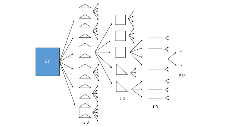
Figure 1: A scheme of recursive reduction of 4D integrals to sums of lower dimensional integrals.

Fig. 1 shows the scheme, where the Gauss’ divergence theorem is applied at each dimension reduction step. Note that while $h_{4}$ is common to all domains, $h_{d}$ for $d<4$ (as well as $\mathbf{a}_{i}$ and $\mathbf{e}_{d}$) are specific to each domain. “Child” domains of dimension $d$ inherit the values of parameters $h_{d+1},h_{d+2},...$ from “parents” and add domain specific $h_{d}$ to the list, which they pass to “children.” We use permutation of variables $s_{1},...,s_{d}$ to reduce the number of integrals over faces $B_{\left(d-1\right)j}$ to a minimum. Integrand transformations on dimensionality reduction can be described as

(35) $$G_{d-1}\left(R_{d-1}\right)=F_{d}\left(P_{d}\right),\quad R_{d-1}^{2}=P_{d}^{2}=R_{d}^{2}-h_{d}^{2},\quad d=4,3,2,1.$$

With (18) and (26) a recursive process is created, and the final PBF is

(36) $$F_{1}\left(P_{1};h_{1},h_{2},h_{3},h_{4}\right)=$$

$$\frac{1}{P_{1}}\int_{0}^{P_{1}}\!\!\!\!\!\!\frac{1}{p_{1}^{2}+h_{1}^{2}}\int_{0}^{\sqrt{p_{1}^{2}+h_{1}^{2}}}\!\!\!\!\!\!\!\!\!\!\!\!\frac{p_{2}}{\left(p_{2}^{2}+h_{2}^{2}\right)^{\frac{3}{2}}}\int_{0}^{\sqrt{p_{2}^{2}+h_{2}^{2}}}\!\!\!\!\!\!\!\!\!\!\frac{p_{3}^{2}}{\left(p_{3}^{2}+h_{3}^{2}\right)^{2}}\int_{0}^{\sqrt{p_{3}^{2}+h_{3}^{2}}}\!\!\!\!p_{4}^{3}G_{4}\left(\sqrt{p_{4}^{2}+h_{4}^{2}}\right)dp_{4}...dp_{1}.$$

All integrals for the free space Green’s function of the Laplace equation can be calculated analytically. At the end of the reduction process the 1D domains are nothing but unit segments $s_{1}\in\left[0,1\right]$. From (20) and (28) we have

$$I_{1}\left(h_{1},h_{2},h_{3},h_{4}\right)=\left(1+s_{10}\right)F_{1}\left(P_{1}\left(1\right);h_{1},h_{2},h_{3},h_{4}\right)-s_{10}F_{1}\left(P_{1}\left(0\right);h_{1},h_{2},h_{3},h_{4}\right),$$

(37) $$P_{1}\left(s_{1}\right)=\left|s_{1}+s_{10}\right|\left|\mathbf{a}_{1}\right|.$$

The recursive process and analytical expressions for (26) or (36) are described next.

3.3 Primitive boundary functions

We provide analytical expressions for PBF $F_{d}\left(P_{d};h_{d},...,h_{4}\right)$. Besides $P_{d}$ these functions depend on $h_{d},...,h_{4}$ only. Some of the parameters are zero, which leads to a substantial simplification of the expressions. We first prove several simple lemmas and specify all possible cases, and then provide expressions for PBFs for each case.

3.3.1 Parameters $h_{d}$

Lemma 3.1.

In the set of parameters $\left\{h_{1},...,h_{4}\right\}$ at least two parameters are zero.

Proof 3.2.

The method the projections are constructed (see (14) and (16)) shows

(38) $$\mathbf{R}_{4}=\mathbf{e}_{4\mathbf{\perp}}+\mathbf{R}_{3}=\mathbf{e}_{4\mathbf{\perp}}+\mathbf{e}_{3\bot}+\mathbf{R}_{2}=...=\mathbf{e}_{4\mathbf{\perp}}+\mathbf{e}_{3\bot}+\mathbf{e}_{2\perp}+\mathbf{e}_{1\bot}+\mathbf{P}_{1},$$

with $h_{d}=\left\|\mathbf{e}_{d\bot}\right\|,\quad d=1,...,4$. By construction all $\mathbf{e}_{d\bot}$ are perpendicular to each other and also to $\mathbf{P}_{1}$. Since these five vectors lie in 3D space, two of them should be zero. However, $P_{1}=\left\|\mathbf{P}_{1}\right\|\neq 0$ (as the final integration is taken over some edge - a segment of finite length), so, at least two of vectors $\mathbf{e}_{d\bot}$ are zero.

Lemma 3.3.

In the set $\left\{h_{1},h_{2},h_{3}\right\}$ at least one is nonzero. So, $h_{1}+h_{2}+h_{3}\neq 0.$

Proof 3.4.

Independent of $h_{4}$, $\mathbf{R}_{3}$ has at least two non-zero components belonging to $span\left(\mathbf{X}_{s},\mathbf{X}_{t}\right)$ or to $span\left(\mathbf{Y}_{u},\mathbf{Y}_{v}\right)$. As $\mathbf{R}_{3}$ can be expanded over 4 vectors and $\mathbf{P}_{1}$ in (38) is not zero, at least one of $\mathbf{e}_{d\bot}$, $d=1,...,3$ is not zero.

Remark 3.5.

As follows from these two lemmas either two or three parameters $\left\{h_{1},...,h_{4}\right\}$ are zero.

Lemma 3.6.

$h_{3}h_{4}=0$.

Proof 3.7.

Indeed, if $h_{4}\neq 0$ then the planes $P_{x}$ and $P_{y}$ containing triangles $S_{x}$ and $S_{y}$ are parallel. In this case, $\mathbf{e}_{3}=$ $\mathbf{e}_{4\mathbf{\|}}\in span\left(\mathbf{X}_{s},\mathbf{X}_{t}\right)=span\left(\mathbf{Y}_{u},\mathbf{Y}_{v}\right)$. Since any three out of four vectors $\mathbf{X}_{s},\mathbf{X}_{t}$,$\mathbf{Y}_{u},\mathbf{Y}_{v}$ generate exactly $span\left(\mathbf{X}_{s},\mathbf{X}_{t}\right)$, then $\mathbf{e}_{3||}$ belongs to the same subspace as $\mathbf{e}_{3}$ and $\mathbf{e}_{3\bot}=\mathbf{0}$.

Lemma 3.8.

$h_{1}+h_{2}\neq 0.$

Proof 3.9.

If $h_{3}=0$ then Lemma (2) provides $h_{1}+h_{2}\neq 0$. If $h_{3}\neq 0$ then according to Lemma (3) we have $h_{4}=0$. The latter shows that planes $P_{x}$ and $P_{y}$ containing triangles $S_{x}$ and $S_{y}$ are not parallel and $span\left(\mathbf{X}_{s},\mathbf{X}_{t},\mathbf{Y}_{u},\mathbf{Y}_{v}\right)$ $=\mathbb{R}^{3}$. So, in representation (38) of $\mathbf{R}_{4}$ at least three out of five $\left\{\mathbf{e}_{4\bot},\mathbf{e}_{3\bot},\mathbf{e}_{2\bot},\mathbf{e}_{1\bot},\mathbf{P}_{1}\right\}$ are nonzero. As $\mathbf{e}_{4\bot}=\mathbf{0},\mathbf{e}_{3\bot}\neq\mathbf{0}$, and $\mathbf{P}_{1}\neq\mathbf{0}$ one of the vectors $\left\{\mathbf{e}_{2\bot},\mathbf{e}_{1\bot}\right\}$ should be nonzero.

As a result only the following cases of parameters $\left\{h_{1},...,h_{4}\right\}$ are possible:

(39) $$\#1\quad h_{4} =h_{3}=h_{2}=0,\quad h_{1}\neq 0,\quad\quad\quad\#2\quad h_{4}=h_{3}=h_{1}=0,\quad h_{2}\neq 0,$$

$$\quad\#3\quad h_{4} =h_{3}=0,\quad h_{2}\neq 0,\quad h_{1}\neq 0,\quad\#4\quad h_{4}=h_{2}=0,\quad h_{3}\neq 0,\quad h_{1}\neq 0,$$

$$\#5\quad h_{4} =h_{1}=0,\quad h_{3}\neq 0,\quad h_{2}\neq 0,\quad\#6\quad h_{3}=h_{2}=0,\quad h_{4}\neq 0,\quad h_{1}\neq 0,$$

$$\#7\quad h_{3} =h_{1}=0,\quad h_{4}\neq 0,\quad h_{2}\neq 0.\quad\quad$$

Some of the typical situations are illustrated in Fig. 2.

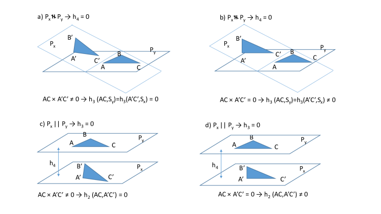
Figure 2: Illustration of typical cases determined by the location of the source ($S_{x}$) and receiver ($S_{y}$) triangles residing in planes $P_{x}$ and $P_{y}$, respectively.

3.3.2 PBF for 4D integral

For the single layer potential we have

(40) $$G_{4}\left(R_{4}\right)=R_{4}^{-1}.$$

General expression for the PBF for $d=4$ is (see (26))

(41) $$F_{4}\left(P_{4};h_{4}\right)=\frac{1}{3P_{4}^{4}}\left[\left(P_{4}^{2}-2h_{4}^{2}\right)R_{4}+2h_{4}^{3}\right],\quad R_{4}=\sqrt{P_{4}^{2}+h_{4}^{2}}.$$

We do not provide derivation of formulae like this, as all obtained expressions can be reduced to tabulated integrals of elementary functions. A simple way to check the validity of the expressions is to differentiate them and check that (24) is satisfied (or differentiate $P_{d}^{d}F_{d}$ and check that the result is $G_{d}\left(R_{d}\right)$). An important case is $h_{4}=0.$ It can be obtained by setting $h_{4}=0$ in (41), or by using (27),

(42) $$F_{4}\left(P_{4};0\right)=\frac{1}{3P_{4}}=\frac{1}{3}G_{4}(R_{4}),\quad R_{4}=P_{4}.$$

So (42) can be used for cases 1-5, while (41) for cases 6-7 in (39).

3.3.3 PBF for 3D integrals

Here, at least one of the parameters $h_{3}$ and $h_{4}$ is zero. Using (26) and (27) for $G_{3}\left(R_{3}\right)=F_{4}\left(P_{4}\right)$ and $d=3$, we obtain for the cases listed in (39)

(43) $$\#1,\#2,\#3:\quad F_{3}\left(P_{3};0,0\right) =\frac{1}{6P_{3}},$$

$$\#4,\#5:\quad F_{3}\left(P_{3};h_{3},0\right) =\frac{1}{6P_{3}^{3}}\left(P_{3}R_{3}-h_{3}^{2}\ln\frac{P_{3}+R_{3}}{h_{3}}\right),\quad R_{3}=\sqrt{P_{3}^{2}+h_{3}^{2}},$$

$$\#6,\#7:\quad F_{3}\left(P_{3};0,h_{4}\right) =\frac{1}{6P_{3}^{3}}\left(P_{3}R_{4}-3h_{4}^{2}\ln\frac{P_{3}+R_{4}}{h_{4}}+4h_{4}^{2}\frac{R_{4}-h_{4}}{P_{3}}\right),$$

$$R_{4} =\sqrt{P_{3}^{2}+h_{4}^{2}}.$$

3.3.4 PBF for 2D integrals

Now in (43) we substitute $G_{2}\left(R_{2}\right)=F_{3}\left(P_{3}\right)$ and use (26) and (27) at $d=2$ to obtain the following expressions for the cases listed in (39)

(44) $$\#1:\quad F_{2}\left(P_{2};0,0,0\right)=\frac{1}{6P_{2}},\quad\#2,\#3:\quad F_{2}\left(P_{2};h_{2},0,0\right)=\frac{R_{2}-h_{2}}{6P_{2}^{2}},$$

$$\#4:\quad F_{2}\left(P_{2};0,h_{3},0\right)=\frac{1}{6P_{2}^{2}}\left[R_{3}-2h_{3}+\frac{h_{3}^{2}}{P_{2}}\ln\frac{P_{2}+R_{3}}{h_{3}}\right],\quad$$

$$\#5:\quad F_{2}\left(P_{2};h_{2},h_{3},0\right)=\frac{1}{6P_{2}^{2}}\left[R_{3}-C_{5}+\frac{h_{3}^{2}}{R_{2}}\ln\frac{R_{2}+R_{3}}{h_{3}}\right],$$

$$\#6:\quad F_{2}\left(P_{2};0,0,h_{4}\right)=\frac{1}{6P_{2}^{2}}\left[R_{4}-3h_{4}+h_{4}^{2}\left(\frac{3}{P_{2}}\ln\frac{P_{2}+R_{4}}{h_{4}}-2\frac{R_{4}-h_{4}}{P_{2}^{2}}\right)\right],\quad$$

$$\#7:\quad F_{2}\left(P_{2};h_{2},0,h_{4}\right)=\frac{1}{6P_{2}^{2}}\left[R_{4}-C_{7}+h_{4}^{2}\left(\frac{3}{R_{2}}\ln\frac{R_{2}+R_{4}}{h_{4}}-2\frac{R_{4}-h_{4}}{R_{2}^{2}}\right)\right],$$

$$h=\sqrt{h_{2}^{2}+h_{3}^{2}+h_{4}^{2}},\quad R_{3}=\sqrt{P_{2}^{2}+h_{2}^{2}+h_{3}^{2}},\quad R_{4}=\sqrt{P_{2}^{2}+h_{2}^{2}+h_{3}^{2}+h_{4}^{2}},$$

$$R_{2}=\sqrt{P_{2}^{2}+h_{2}^{2}},\quad C_{5}=h+\frac{h_{3}^{2}}{h_{2}}\ln\frac{h_{2}+h}{h_{3}},\quad\!\!\!C_{7}=h+h_{4}^{2}\left(\frac{3}{h_{2}}\ln\frac{h_{2}+h}{h_{4}}-2\frac{h-h_{4}}{h_{2}^{2}}\right).$$

3.3.5 PBF for 1D integrals

Similarly, by setting $G_{1}\left(R_{1}\right)=F_{2}\left(P_{2}\right)$ and using (26) at $d=1$ we obtain

(45) $$\#1:\quad F_{1}\left(P_{1};h_{1},0,0,0\right)=\frac{1}{6}\Phi_{1}\left(P_{1}\right),$$

$$\#2:\quad F_{1}\left(P_{1};0,h_{2},0,0\right)=\frac{1}{6}\left(\Phi_{1}\left(P_{1}\right)-\frac{1}{R_{2}+h_{2}}\right),$$

$$\#3:\quad F_{1}\left(P_{1};h_{1},h_{2},0,0\right)=\frac{1}{6}\left[\Phi_{1}\left(P_{1}\right)-\frac{h_{2}}{h_{1}}\Phi_{2}\left(P_{1};h_{1}\right)\right],$$

$$\#4:\quad F_{1}\left(P_{1};h_{1},0,h_{3},0\right)=\frac{1}{6}\left[\left(1-\frac{h_{3}^{2}}{h_{1}^{2}}\right)\Phi_{1}\left(P_{1}\right)-\frac{2h_{3}}{h_{1}}\Phi_{2}\left(P_{1};h_{1}\right)+\frac{h_{3}^{2}}{h_{1}^{2}}\Phi_{3}\left(P_{1}\right)\right],\quad$$

$$\#5:\quad F_{1}\left(P_{1};0,h_{2},h_{3},0\right)=\frac{1}{6}\left[\frac{h^{2}}{h_{2}^{2}}\Phi_{1}\left(P_{1}\right)-\frac{1}{R_{4}+h}-\Phi_{4}\left(P_{1};h_{3}\right)\right],\quad$$

$$\#6:\quad F_{1}\left(P_{1};h_{1},0,0,h_{4}\right)=$$

$$\quad\frac{1}{6}\left[\left(1-\frac{3h_{4}^{2}}{h_{1}^{2}}\right)\Phi_{1}\left(P_{1}\right)-\left(3-\frac{h_{4}^{2}}{h_{1}^{2}}\right)\frac{h_{4}}{h_{1}}\Phi_{2}\left(P_{1};h_{1}\right)+3\frac{h_{4}^{2}}{h_{1}^{2}}\Phi_{3}\left(P_{1}\right)-\frac{h_{4}^{2}}{h_{1}^{2}\left(R_{4}+h_{4}\right)}\right],$$

$$\#7:\quad F_{1}\left(P_{1};0,h_{2},0,h_{4}\right)$$

$$\quad\quad\quad=\frac{1}{6}\left[\left(1+\frac{3h_{4}^{2}}{h_{2}^{2}}\right)\Phi_{1}\left(P_{1}\right)-\frac{2h_{4}^{3}}{h_{2}^{3}}\Phi_{2}\left(P_{1};h_{2}\right)-3\Phi_{4}\left(P_{1};h_{4}\right)+\frac{2h_{4}^{2}-h_{2}^{2}}{h_{2}^{2}\left(R_{4}+h\right)}\right],$$

$$R_{4}=\sqrt{P_{1}^{2}+h^{2}},\quad R_{1}=\sqrt{P_{1}^{2}+h_{1}^{2}},\quad R_{2}=\sqrt{P_{1}^{2}+h_{2}^{2}},\quad h^{2}=h_{1}^{2}+h_{2}^{2}+h_{3}^{2}+h_{4}^{2},$$

$$\Phi_{1}\left(P_{1}\right)=\frac{1}{P_{1}}\ln\frac{P_{1}+R_{4}}{h},\quad\Phi_{2}\left(P_{1};\eta\right)=\frac{1}{P_{1}}\arctan\frac{\eta P_{1}}{h^{2}+R_{4}\sqrt{h^{2}-\eta^{2}}},$$

$$\Phi_{3}\left(P_{1}\right)=\frac{1}{R_{1}}\ln\frac{R_{1}+R_{4}}{\sqrt{h^{2}-h_{1}^{2}}},\quad\Phi_{4}\left(P_{1};\eta\right)=\frac{\eta^{2}}{P_{1}^{2}h_{2}}\left(\frac{R_{2}}{h_{2}}\ln\frac{R_{2}+R_{4}}{\eta}-\ln\frac{h_{2}+h}{\eta}\right).$$

3.4 Domains and parameters

In this section we specify the domains of integration and parameters, which enable determination of projections and parameters $h_{1},...,h_{4}$. Before doing that we provide a proof of a lemma, which allows us obtain substantial simplifications of analytical expressions.

3.4.1 4D domain and 4D integral

From the parametrization of triangles and (14) and (15) we have for $d=4$

(46) $$s_{1}= s,\quad s_{2}=t,\quad s_{3}=u,\quad s_{4}=v,$$

$$\mathbf{a}_{1}= \mathbf{X}_{s},\text{\quad}\mathbf{a}_{2}=\mathbf{X}_{t},\quad\mathbf{a}_{3}=-\mathbf{Y}_{u},\quad\mathbf{a}_{4}=-\mathbf{Y}_{v},\quad\mathbf{e}_{4}=\mathbf{X}_{0}-\mathbf{Y}_{0}.$$

We are interested in evaluation of integral

(47) $$U=I_{4}\left(\mathbf{a}_{1},\mathbf{a}_{2},\mathbf{a}_{3},\mathbf{a}_{4},\mathbf{e}_{4}\right)=\int_{D_{4}}...$$

$$=\int_{0}^{1}\int_{0}^{1-s_{1}}\int_{0}^{1}\int_{0}^{1-s_{3}}G_{4}\left(R_{4}\left(s_{1},s_{2},s_{3},s_{4};\mathbf{a}_{1},\mathbf{a}_{2},\mathbf{a}_{3},\mathbf{a}_{4},\mathbf{e}_{4}\right)\right)ds_{4}ds_{3}ds_{2}ds_{1}$$

The integration domain $D_{4}$ is the Cartesian product of standard triangles, $T_{x}\otimes$ $T_{y}$.

3.4.2 4D domain boundaries and 3D integrals

The boundaries of domain $D_{4}$ consist of 6 right prisms:

(48) $$B_{31} =T_{x}\otimes C_{y1},\quad B_{32}=T_{x}\otimes C_{y2},\quad B_{33}=T_{x}\otimes C_{y3},$$

$$B_{34} =C_{x1}\otimes T_{y},\quad B_{35}=C_{x2}\otimes T_{y},\quad B_{36}=C_{x3}\otimes T_{y},$$

where $C_{xj}$ and $C_{yj}$, $j=1,2,3$ are the edges of triangles $T_{x}$ and $T_{y}$, respectively. (20) and (28) then provide

(49) $$U= I_{4}\left(\mathbf{a}_{1},\mathbf{a}_{2},\mathbf{a}_{3},\mathbf{a}_{4},\mathbf{e}_{4}\right)=\sum_{j=1}^{6}I_{3j},$$

$$I_{31}= -s_{40}\int_{B_{31}}F_{4}\left(P_{4}\left(s_{1},s_{2},s_{3},0\right)\right)ds_{1}ds_{2}ds_{3}=-s_{40}I_{3}\left(\mathbf{a}_{11},\mathbf{a}_{21},\mathbf{a}_{31},\mathbf{e}_{31}\right),$$

$$I_{32}= \left(1+s_{30}+s_{40}\right)\int_{B_{32}}F_{4}\left(P_{4}\left(s_{1},s_{2},1-s_{4},s_{4}\right)\right)ds_{1}ds_{2}ds_{4}$$

$$= \left(1+s_{30}+s_{40}\right)I_{3}\left(\mathbf{a}_{12},\mathbf{a}_{22},\mathbf{a}_{32},\mathbf{e}_{32}\right),$$

$$I_{33}= -s_{30}\int_{B_{33}}F_{4}\left(P_{4}\left(s_{1},s_{2},0,s_{4}\right)\right)ds_{1}ds_{2}ds_{4}=-s_{30}I_{3}\left(\mathbf{a}_{13},\mathbf{a}_{23},\mathbf{a}_{33},\mathbf{e}_{33}\right),$$

$$I_{34}= -s_{20}\int_{B_{34}}F_{4}\left(P_{4}\left(s_{1},0,s_{3},s_{4}\right)\right)ds_{1}ds_{3}ds_{4}=-s_{20}I_{3}\left(\mathbf{a}_{14},\mathbf{a}_{24},\mathbf{a}_{34},\mathbf{e}_{34}\right),$$

$$I_{35}= \left(1+s_{10}+s_{20}\right)\int_{B_{35}}F_{4}\left(P_{4}\left(1-s_{2},s_{2},s_{3},s_{4}\right)\right)ds_{2}ds_{3}ds_{4}$$

$$= \left(1+s_{10}+s_{20}\right)I_{3}\left(\mathbf{a}_{15},\mathbf{a}_{25},\mathbf{a}_{35},\mathbf{e}_{35}\right),$$

$$I_{36}= -s_{10}\int_{B_{36}}F_{4}\left(P_{4}\left(0,s_{2},s_{3},s_{4}\right)\right)ds_{2}ds_{3}ds_{4}=-s_{10}I_{3}\left(\mathbf{a}_{16},\mathbf{a}_{26},\mathbf{a}_{36},\mathbf{e}_{36}\right).$$

Here $D_{3}$ is a right prism in 3D space (the same as $B_{31}$), so

(50) $$I_{3}\left(\mathbf{a}_{1j},\mathbf{a}_{2j},\mathbf{a}_{3j},\mathbf{e}_{3j}\right)=\!\!\int_{D_{3}}\!\!\!\!\!...=\!\!\int_{0}^{1}\!\!\!\int_{0}^{1-s_{1}}\!\!\!\!\int_{0}^{1}\!\!\!G_{3}\left(R_{3}\left(s_{1},s_{2},s_{3};\mathbf{a}_{1j},\mathbf{a}_{2j},\mathbf{a}_{3j},\mathbf{e}_{3j}\right)\right)ds_{3}ds_{2}ds_{1}.$$

Parameters of the 3D integral follow from the integration domain (to avoid confusion we extend the subscript of parameters of these integrals to add the index $j=1,...,6$ of the integral at the end),

(51) $$\mathbf{a}_{11} =\mathbf{a}_{1}\mathbf{,\quad a}_{21}=\mathbf{a}_{2}\mathbf{,\quad a}_{31}=\mathbf{a}_{3}\mathbf{,\quad a}_{12}=\mathbf{a}_{1}\mathbf{,\quad a}_{22}=\mathbf{a}_{2}\mathbf{,\quad a}_{32}=\mathbf{a}_{4}-\mathbf{a}_{3}\mathbf{,}$$

$$\mathbf{a}_{13} =\mathbf{a}_{1}\mathbf{,\quad a}_{23}=\mathbf{a}_{2}\mathbf{,\quad a}_{33}=\mathbf{a}_{4}\mathbf{,\quad a}_{14}=\mathbf{a}_{3}\mathbf{,\quad a}_{24}=\mathbf{a}_{4}\mathbf{,\quad a}_{34}=\mathbf{a}_{1}\mathbf{,}$$

$$\mathbf{a}_{15} =\mathbf{a}_{3}\mathbf{,\quad a}_{25}=\mathbf{a}_{4}\mathbf{,\quad a}_{35}=\mathbf{a}_{2}-\mathbf{a}_{1}\mathbf{,\quad a}_{16}=\mathbf{a}_{3}\mathbf{,\quad a}_{26}=\mathbf{a}_{4}\mathbf{,\quad a}_{36}=\mathbf{a}_{2}\mathbf{,}$$

$$\mathbf{e}_{31} =\mathbf{e}_{33}=\mathbf{e}_{34}=\mathbf{e}_{36}=\sum_{d=1}^{4}\mathbf{a}_{d}s_{d0},\quad\mathbf{e}_{32}=\mathbf{e}_{31}+\mathbf{a}_{3},\quad\mathbf{e}_{35}=\mathbf{e}_{31}+\mathbf{a}_{1},\quad$$

where the values for parameters $\mathbf{a}_{1},\mathbf{a}_{2},\mathbf{a}_{3},\mathbf{a}_{4}$ of the 4D integrals are provided by (46) and coordinates of projections $s_{10},...,s_{40}$ and $h_{4}$ can be found from these parameters and $\mathbf{e}_{4}$ (see Appendix).

3.4.3 3D domain boundaries and 2D integrals

The prism $D_{3}$ has 3 rectangular faces and 2 triangular faces. Rectangles are located in planes $s_{1}+s_{2}=1$, $s_{1}=0$,  and $s_{2}=0$, and triangles are located in planes $s_{3}=1$ and $s_{3}=0$ (see (50)). So, we have

(52) $$I_{3}\left(\mathbf{a}_{1},\mathbf{a}_{2},\mathbf{a}_{3},\mathbf{e}_{3}\right)=\sum_{j=1}^{5}I_{2j},$$

$$I_{21}=\left(1+s_{10}+s_{20}\right)\int_{0}^{1}\int_{0}^{1}F_{3}\left(P_{3}\left(s_{1},1-s_{1},s_{3}\right)\right)ds_{1}ds_{3}=\left(1+s_{10}+s_{20}\right)I_{2}^{(s)}\left(\mathbf{a}_{11},\mathbf{a}_{21},\mathbf{e}_{21}\right),$$

$$I_{22}=-s_{10}\int_{0}^{1}\int_{0}^{1}F_{3}\left(P_{3}\left(0,s_{2},s_{3}\right)\right)ds_{2}ds_{3}=-s_{10}I_{2}^{(s)}\left(\mathbf{a}_{12},\mathbf{a}_{22},\mathbf{e}_{22}\right),$$

$$I_{23}=-s_{20}\int_{0}^{1}\int_{0}^{1}F_{3}\left(P_{3}\left(s_{1},0,s_{3}\right)\right)ds_{1}ds_{3}=-s_{20}I_{2}^{(s)}\left(\mathbf{a}_{13},\mathbf{a}_{23},\mathbf{e}_{23}\right),$$

$$I_{24}=\left(1+s_{30}\right)\int_{0}^{1}\int_{0}^{1-s_{1}}F_{3}\left(P_{3}\left(s_{1},s_{2},1\right)\right)ds_{2}ds_{1}=\left(1+s_{30}\right)I_{2}^{(t)}\left(\mathbf{a}_{14},\mathbf{a}_{24},\mathbf{e}_{24}\right),$$

$$I_{25}=-s_{30}\int_{0}^{1}\int_{0}^{1-s_{1}}F_{3}\left(P_{3}\left(s_{1},s_{2},0\right)\right)ds_{2}ds_{1}=-s_{30}I_{2}^{(t)}\left(\mathbf{a}_{15},\mathbf{a}_{25},\mathbf{e}_{25}\right).$$

We use standardization of 2D domains, which are square (superscript “$s$”) and triangle (superscript “$t$”),

(53) $$I_{2}^{(s)}\left(\mathbf{a}_{1j},\mathbf{a}_{2j},\mathbf{e}_{2j}\right) =\int_{D_{2}^{(s)}}...=\int_{0}^{1}\int_{0}^{1}G_{2}\left(R_{2}\left(s_{1},s_{2};\mathbf{a}_{1j},\mathbf{a}_{2j},\mathbf{e}_{2j}\right)\right)ds_{2}ds_{1},$$

$$I_{2}^{(t)}\left(\mathbf{a}_{1j},\mathbf{a}_{2j},\mathbf{e}_{2j}\right) =\int_{D_{2}^{(t)}}...=\int_{0}^{1}\int_{0}^{1-s_{1}}G_{2}\left(R_{2}\left(s_{1},s_{2};\mathbf{a}_{1j},\mathbf{a}_{2j},\mathbf{e}_{2j}\right)\right)ds_{2}ds_{1}.$$

Note that $s_{10},s_{20},s_{30}$, and $h_{3}$ can be found from parameters of $I_{3}$ in (52) (see Appendix), while parameters of the 2D integrals are related to these parameters as

(54) $$\mathbf{a}_{11} =\mathbf{a}_{1}-\mathbf{a}_{2},\quad\mathbf{a}_{21}=\mathbf{a}_{3},\quad\mathbf{a}_{12}=\mathbf{a}_{2},\quad\mathbf{a}_{22}=\mathbf{a}_{3},\quad\mathbf{a}_{13}=\mathbf{a}_{1},\quad\mathbf{a}_{23}=\mathbf{a}_{3},$$

$$\mathbf{a}_{14} =\mathbf{a}_{1},\quad\mathbf{a}_{24}=\mathbf{a}_{2},\quad\mathbf{a}_{15}=\mathbf{a}_{1},\quad\mathbf{a}_{25}=\mathbf{a}_{2},\quad\mathbf{e}_{21}=\mathbf{e}_{22}+\mathbf{a}_{2},$$

$$\mathbf{e}_{22} =\mathbf{e}_{23}=\mathbf{e}_{25}=\mathbf{a}_{1}s_{10}+\mathbf{a}_{2}s_{20}+\mathbf{a}_{3}s_{30},\quad\mathbf{e}_{24}=\mathbf{e}_{22}+\mathbf{a}_{3}.\quad$$

3.4.4 2D domain boundaries and 1D integrals

Following the scheme of the previous subsections we can reduce integration over the square and triangle to contour integration consisting of 4 and 3 line integrals, respectively. We have then

(55) $$I_{2}^{(s)}\left(\mathbf{a}_{1},\mathbf{a}_{2},\mathbf{e}_{2}\right)=\sum_{j=1}^{4}I_{1j}^{(s)},\quad I_{2}^{(t)}\left(\mathbf{a}_{1},\mathbf{a}_{2},\mathbf{e}_{2}\right)=\sum_{j=1}^{3}I_{1j}^{(t)},$$

$$I_{11}^{(s)}=\left(1+s_{10}\right)\int_{0}^{1}F_{2}\left(P_{2}\left(1,s_{2}\right)\right)ds_{2}=\left(1+s_{10}\right)I_{1}\left(\mathbf{a}_{11},\mathbf{e}_{11}\right),$$

$$I_{12}^{(s)}=I_{11}^{(t)}=-s_{10}\int_{0}^{1}F_{2}\left(P_{2}\left(0,s_{2}\right)\right)ds_{2}=-s_{10}I_{1}\left(\mathbf{a}_{12},\mathbf{e}_{12}\right),$$

$$I_{13}^{(s)}=\left(1+s_{20}\right)\int_{0}^{1}F_{2}\left(P_{2}\left(s_{1},1\right)\right)ds_{1}=\left(1+s_{20}\right)I_{1}\left(\mathbf{a}_{13},\mathbf{e}_{13}\right),$$

$$I_{14}^{(s)}=I_{12}^{(t)}=-s_{20}\int_{0}^{1}F_{2}\left(P_{2}\left(s_{1},0\right)\right)ds_{1}=-s_{20}I_{1}\left(\mathbf{a}_{14},\mathbf{e}_{14}\right),$$

$$I_{13}^{(t)}=\left(1+s_{10}+s_{20}\right)\int_{0}^{1}F_{2}\left(P_{2}\left(s_{1},1-s_{1}\right)\right)ds_{1}=\left(1+s_{10}+s_{20}\right)I_{1}\left(\mathbf{a}_{15},\mathbf{e}_{15}\right),$$

$$I_{1}\left(\mathbf{a}_{1j},\mathbf{e}_{1j}\right)=\int_{D_{1}}...=\int_{0}^{1}G_{1}\left(R_{1}\left(s_{1};\mathbf{a}_{1j},\mathbf{e}_{1j}\right)\right)ds_{1}.$$

Also, $s_{10},s_{20},$ and $h_{2}$ can be found from parameters of $I_{2}$ in (55) (see Appendix), while parameters of the 1D integrals are related to these parameters as

(56) $$\mathbf{a}_{11} = \mathbf{a}_{12}=\mathbf{a}_{2}\mathbf{,\quad a}_{13}=\mathbf{a}_{14}=\mathbf{a}_{1},\quad\mathbf{a}_{15}=\mathbf{a}_{1}-\mathbf{a}_{2}\mathbf{,}$$

$$\mathbf{e}_{12} = \mathbf{e}_{14}=\mathbf{a}_{1}s_{10}+\mathbf{a}_{2}s_{20},\quad\mathbf{e}_{11}=\mathbf{e}_{12}+\mathbf{a}_{1},\quad\mathbf{e}_{13}=\mathbf{e}_{15}=\mathbf{e}_{12}+\mathbf{a}_{2}.\quad$$

3.4.5 Evaluation of 1D integrals

The integration process ends with evaluation of the 1D integral (also, see (37))

(57) $$I_{1}\left(\mathbf{a}_{1},\mathbf{e}_{1}\right)=\left(1+s_{10}\right)F_{1}\left(P_{1}\left(1\right)\right)-s_{10}F_{1}\left(P_{1}\left(0\right)\right),\quad P_{1}\left(s_{1}\right)=\left|s_{1}+s_{10}\right|\left|\mathbf{a}_{1}\right|,$$

where $F_{1}\left(P_{1}\right)$ is provided by expressions (45) and parameters $s_{10}$ and $h_{1}$ can be found from $\mathbf{a}_{1}$ and $\mathbf{e}_{1}$ as provided in the Appendix.

4 Gradient of single layer and double layer potential

We next consider integrals (2) and (3). We start with the case when $S_{x}$ and $S_{y}$ do not have common points, $S_{x}\cap S_{y}=\emptyset$. In this case integral $M$ does not require a special treatment, since $M=$ $-\mathbf{n}_{x}\cdot\mathbf{L}^{\prime}$. Indeed, due to the symmetry property of $G\left(\mathbf{x,y}\right)$ (5), we have

(58) $$\mathbf{L}^{\prime}=\int_{S_{y}}\int_{S_{x}}\nabla_{\mathbf{y}}G\left(\mathbf{x,y}\right)dS\left(\mathbf{x}\right)dS\left(\mathbf{y}\right)=-\int_{S_{y}}\int_{S_{x}}\nabla_{\mathbf{x}}G\left(\mathbf{x,y}\right)dS\left(\mathbf{x}\right)dS\left(\mathbf{y}\right).$$

Note that the gradient can be decomposed into the surface gradient and normal derivative operators:

(59) $$\nabla_{\mathbf{x}}=\nabla_{s\mathbf{x}}+\mathbf{n}_{x}\left(\mathbf{n}_{x}\cdot\nabla_{\mathbf{x}}\right),\quad\nabla_{\mathbf{y}}=\nabla_{s\mathbf{y}}+\mathbf{n}_{y}\left(\mathbf{n}_{y}\cdot\nabla_{\mathbf{y}}\right).$$

This shows that two forms of the integral in (58) can be written as

(60) $$\mathbf{L}^{\prime} = \mathbf{F}_{y}+\mathbf{n}_{y}L_{y}^{\prime},\quad\mathbf{L}^{\prime}=-\mathbf{F}_{x}+\mathbf{n}_{x}L_{x}^{\prime},\quad$$

$$L_{y}^{\prime} = \mathbf{n}_{y}\cdot\mathbf{L}^{\prime},\quad\mathbf{F}_{y}=\int_{S_{x}}\int_{S_{y}}\nabla_{s\mathbf{y}}G\left(\mathbf{x,y}\right)dS\left(\mathbf{y}\right)dS\left(\mathbf{x}\right),$$

$$L_{x}^{\prime} = \mathbf{n}_{x}\cdot\mathbf{L}^{\prime},\quad\mathbf{F}_{x}=\int_{S_{y}}\int_{S_{x}}\nabla_{s\mathbf{x}}G\left(\mathbf{x,y}\right)dS\left(\mathbf{x}\right)dS\left(\mathbf{y}\right).$$

Taking the scalar product of the first equation with $\mathbf{n}_{x}$ and the second equation with $\mathbf{n}_{y}$, we obtain simultaneous equations with respect to $L_{x}^{\prime}$ and $L_{y}^{\prime},$

(61) $$L_{x}^{\prime}=\mathbf{n}_{x}\cdot\mathbf{F}_{y}+\left(\mathbf{n}_{x}\cdot\mathbf{n}_{y}\right)L_{y}^{\prime},\quad L_{y}^{\prime}=-\mathbf{n}_{y}\cdot\mathbf{F}_{x}+\left(\mathbf{n}_{x}\cdot\mathbf{n}_{y}\right)L_{x}^{\prime}.\\$$

This system is non-degenerate unless the planes $P_{x}$ and $P_{y}$ containing triangles $S_{x}$ and $S_{y}$ are parallel ($\left|\mathbf{n}_{x}\cdot\mathbf{n}_{y}\right|=1$). Below we consider both, the non-degenerate and degenerate cases. Before that we note that integrals $\mathbf{F}_{x}$ and $\mathbf{F}_{y}$ can be reduced to 3D integrals using the Gauss’ theorem,

(62) $$\mathbf{F}_{x}= \int_{S_{y}}\int_{C_{x}}\mathbf{n}_{cx}G\left(\mathbf{x,y}\right)dC\left(\mathbf{x}\right)dS\left(\mathbf{y}\right)=\sum_{i=1}^{3}\mathbf{n}_{cxi}F_{xi},$$

$$F_{xi}= \int_{S_{y}}\int_{C_{xi}}G\left(\mathbf{x,y}\right)dC\left(\mathbf{x}\right)dS\left(\mathbf{y}\right),\quad\mathbf{n}_{cxi}=\frac{\left(\mathbf{l}_{xi}\times\mathbf{n}_{x}\right)}{l_{xi}},\quad\mathbf{n}_{x}=-\frac{\mathbf{l}_{x1}\times\mathbf{l}_{x3}}{2A_{x}},$$

$$\mathbf{F}_{y}= \int_{S_{x}}\int_{C_{y}}\mathbf{n}_{cy}G\left(\mathbf{x,y}\right)dC\left(\mathbf{y}\right)dS\left(\mathbf{x}\right)=\sum_{i=1}^{3}\mathbf{n}_{cyi}F_{yi},$$

$$F_{yi}= \int_{S_{x}}\int_{C_{yi}}G\left(\mathbf{x,y}\right)dC\left(\mathbf{y}\right)dS\left(\mathbf{x}\right),\quad\mathbf{n}_{cyi}=\frac{\mathbf{l}_{yi}\times\mathbf{n}_{y}}{l_{yi}},\quad\mathbf{n}_{y}=-\frac{\mathbf{l}_{y1}\times\mathbf{l}_{y3}}{2A_{y}}.$$

Here $\mathbf{n}_{cx}$ and $\mathbf{n}_{cy}$ are the outer normals to contours $C_{x}$ and $C_{y}$ bounding triangles $S_{x}$ and $S_{y}$, respectively. These contours consist of segments $C_{xi}$ and $C_{yi}$ with normals $\mathbf{n}_{cxi}$ and $\mathbf{n}_{cyi}$, $i=1,2,3.$

So, we have six scalar integrals (62), which are nothing, but integrals over prismatic domains (48) where

(63) $$F_{yi}=2l_{yi}A_{x}\widetilde{I}_{3}\left(\mathbf{a}_{1i},\mathbf{a}_{2i},\mathbf{a}_{3i},\mathbf{e}_{3i}\right),\quad F_{xi}=2l_{xi}A_{y}\widetilde{I}_{3}\left(\mathbf{a}_{1j},\mathbf{a}_{2j},\mathbf{a}_{3j},\mathbf{e}_{3j}\right),$$

for $i=1,2,3$, $j=i+3$, and $\widetilde{I}_{3}$ is defined as

(64) $$\widetilde{I}_{3}\left(\mathbf{a}_{1j},\mathbf{a}_{2j},\mathbf{a}_{3j},\mathbf{e}_{3j}\right)=\int_{D_{3}}...=\int_{0}^{1}\int_{0}^{1-s_{1}}\int_{0}^{1}\widetilde{G}_{3}\left(R_{3}\left(s_{1},s_{2},s_{3};\mathbf{a}_{1j},\mathbf{a}_{2j},\mathbf{a}_{3j},\mathbf{e}_{3j}\right)\right)ds_{3}ds_{2}ds_{1},$$

$$\widetilde{G}_{3}\left(R_{3}\right)=\left(R_{3}^{2}+h_{4}^{2}\right)^{-1/2}=G_{4}\left(R_{4}\right)=R_{4}^{-1},$$

and parameters $\mathbf{a}_{1j},\mathbf{a}_{2j},\mathbf{a}_{3j},\mathbf{e}_{3j}$, $j=1,...,6$ are provided by (51), where the values for parameters $\mathbf{a}_{1},\mathbf{a}_{2},\mathbf{a}_{3},\mathbf{a}_{4}$ of the 4D integrals are provided by (46) and coordinates of projections $s_{10},...,s_{40}$ and $h_{4}$ can be found from these parameters and $\mathbf{e}_{4}$ in the same way as for the single layer potential. So, the integrals $I_{3}$ and $\widetilde{I}_{3}$ depend on the same parameter set, but have different integrands.

4.1 Non-degenerate case

Solving the system for the non-degenerate case we get

(65) $$-M=L_{x}^{\prime}=\frac{\mathbf{n}_{x}\cdot\mathbf{F}_{y}-\left(\mathbf{n}_{x}\cdot\mathbf{n}_{y}\right)\mathbf{n}_{y}\cdot\mathbf{F}_{x}}{1-\left(\mathbf{n}_{x}\cdot\mathbf{n}_{y}\right)^{2}},\quad\mathbf{L}^{\prime}=-\mathbf{F}_{x}+\mathbf{n}_{x}L_{x}^{\prime}=-\mathbf{F}_{x}-\mathbf{n}_{x}M.$$

This shows that it is sufficient to compute integrals $\mathbf{F}_{x}$ and $\mathbf{F}_{y}$ to obtain the values of integrals (2) - (3) in the non-degenerate case. The non-degenerate case corresponds to $\left|\mathbf{n}_{x}\cdot\mathbf{n}_{y}\right|\neq 1$, so $P_{x}$ and $P_{y}$ are not parallel and $h_{4}=0$. Note that in this case we have (see (42) and (50))

(66) $$\widetilde{G}_{3}\left(R_{3}\right)=3G_{3}\left(R_{3}\right),\quad\widetilde{I}_{3}\left(\mathbf{a}_{1j},\mathbf{a}_{2j},\mathbf{a}_{3j},\mathbf{e}_{3j}\right)=3I_{3}\left(\mathbf{a}_{1j},\mathbf{a}_{2j},\mathbf{a}_{3j},\mathbf{e}_{3j}\right).$$

Hence, if one needs to compute integrals (1) - (3) for the most common situation $h_{4}=0$, integrals (2) - (3) come for almost no additional cost.

4.2 Degenerate case

Note that after $M$ is computed $\mathbf{L}^{\prime}$ can be found from the last equation (65. There are two problems that need to be resolved for the degenerate case. First, how to compute $M$ as the method presented by (65) does not work in this case. Second, how to evaluate integrals (64) at $h_{4}\neq 0$.

4.2.1 Evaluation of $M$

In case when planes $P_{x}$ and $P_{y}$ are parallel we can consider the function

(67) $$G^{\prime}\left(\mathbf{x,y}\right)=\mathbf{n}_{x}\cdot\nabla_{\mathbf{x}}G\left(\mathbf{x},\mathbf{y}\right)=\frac{\mathbf{n}_{x}\cdot\left(\mathbf{y}-\mathbf{x}\right)}{\left|\mathbf{x}-\mathbf{y}\right|^{3}}=\frac{\delta}{\left|\mathbf{x}-\mathbf{y}\right|^{3}},\quad h_{4}=\left|\delta\right|$$

where constant $\delta$ is a signed distance between the planes of $P_{x}$ and $P_{y}$. So,

(68) $$M=\int_{S_{y}}\int_{S_{x}}G^{\prime}\left(\mathbf{x,y}\right)dS\left(\mathbf{x}\right)dS\left(\mathbf{y}\right)=4A_{x}A_{y}\delta U^{\prime},$$

$$U^{\prime}=\int_{0}^{1}\!\!\int_{0}^{1-u}\!\!\!\int_{0}^{1}\!\!\int_{0}^{1-s}\!\!\!\!\!g^{\prime}\left(s,t,u,v\right)dtdsdvdu,\quad g^{\prime}=\frac{G^{\prime}\left(\mathbf{X}\left(s,t\right)\mathbf{,Y}\left(u,v\right)\right)}{\delta}=\frac{1}{\left|\mathbf{X}-\mathbf{Y}\right|^{3}}.$$

Here and below we use the prime for the integrals related to $M$. It is also clear that at $\delta=0$ we have $G^{\prime}=0$ ($S_{x}$ and $S_{y}$ in the same plane). In fact, this corresponds to the principal value of integral (2) when $\mathbf{y}\in S_{x}$. So, we should set $M=0$ for $\delta=0$.

Now computations of $U^{\prime}$ are similar to computations of $U$ given by (11) with the only difference that instead of (40) we should use PBF

(69) $$G_{4}^{\prime}\left(R_{4}\right)=R_{4}^{-3}$$

and consider only cases #6 and #7 listed in (39). The results of integration for $d=4,3,$ and $2$ are:

(70) $$\#6,7 :\quad F_{4}^{\prime}\left(P_{4};h_{4}\right)=\frac{1}{P_{4}^{4}}\left(\frac{P_{4}^{2}+2h_{4}^{2}}{R_{4}}-2h_{4}\right),\quad R_{4}=\sqrt{P_{4}^{2}+h_{4}^{2}},$$

$$\#6,7 :\quad F_{3}^{\prime}(P_{3};0,h_{4})=\frac{1}{P_{3}^{3}}\left[-\frac{2P_{3}}{R_{4}+h_{4}}+\ln\frac{P_{3}+R_{4}}{h_{4}}\right],\quad R_{4}=\sqrt{P_{3}^{2}+h_{4}^{2}},$$

$$\#6 :\quad\!F_{2}^{\prime}\!\left(P_{2};0,0,h_{4}\right)=\frac{1}{P_{2}^{2}}\!\left[\frac{1}{R_{4}+h_{4}}-\frac{1}{P_{2}}\ln\frac{P_{2}+R_{4}}{h_{4}}+\frac{1}{2h_{4}}\right],\quad\!R_{4}=\sqrt{P_{2}^{2}+h_{4}^{2}},$$

$$\#7 :\quad\!F_{2}^{\prime}\!\left(P_{2};h_{2},0,h_{4}\right)=$$

$$\!\!\frac{1}{P_{2}^{2}}\!\left(\frac{1}{R_{4}+h_{4}}-\frac{1}{h+h_{4}}-\frac{1}{R_{2}}\ln\frac{R_{2}+R_{4}}{h_{4}}+\frac{1}{h_{2}}\ln\frac{h_{2}+h}{h_{4}}\right),\quad R_{4}=\sqrt{P_{2}^{2}+h^{2}},$$

with $h=\sqrt{h_{2}^{2}+h_{4}^{2}}$. For $d=1$ we have

(71) $$\#6: \quad\!\!\!F_{1}^{\prime}\!\left(P_{1};h_{1},0,0,h_{4}\right)=\frac{1}{h_{1}^{2}}\!\!\left[\Phi_{1}\!\left(P_{1}\right)+\frac{h_{1}^{2}-h_{4}^{2}}{2h_{1}h_{4}}\Phi_{2}\!\left(P_{1};h_{1}\right)-\Phi_{3}\!\left(P_{1}\right)+\frac{1}{2\left(R_{4}+h_{4}\right)}\right],$$

$$\#7: \quad\!\!\!F_{1}^{\prime}\!\left(P_{1};0,h_{2},0,h_{4}\right)=\frac{-1}{h_{2}^{2}}\left[\Phi_{1}\left(P_{1}\right)-\frac{h_{4}}{h_{2}}\Phi_{2}\left(P_{1};h_{2}\right)-\frac{h_{2}^{2}}{h_{4}^{2}}\Phi_{4}\left(P_{1};h_{4}\right)+\frac{1}{P_{1}^{2}}\left(\frac{R_{2}^{2}}{R_{4}+h_{4}}-\frac{h_{2}^{2}}{h+h_{4}}\right)\right],$$

where $R_{2},R_{4},\Phi_{1},\Phi_{2},\Phi_{3},$ and $\Phi_{4}$ are provided by (45).

4.2.2 Evaluation of $\mathbf{F}_{x}$

Again, we consider only cases #6 and #7 from (39) for the PBFs generated by $\widetilde{G}_{3}\left(R_{3}\right)$, which we mark with tilde. With $R_{4}=\sqrt{P_{3}^{2}+h_{4}^{2}}$, we have by definition

(72) $$\#6,7:\quad\!\!\!\widetilde{F}_{3}\left(P_{3};0,h_{4}\right)= \frac{1}{P_{3}^{3}}\int_{0}^{P_{3}}\!\!\!\!P^{2}\widetilde{G}_{3}\left(\sqrt{P^{2}+h_{4}^{2}}\right)dP=\frac{R_{4}}{2P_{3}^{2}}-\frac{h_{4}^{2}}{2P_{3}^{3}}\ln\frac{P_{3}+R_{4}}{h_{4}}.$$

Comparing this with (43) we can see that this function coincides with $F_{3}\left(P_{3};h_{3},0\right)$ multiplied by 3, but with parameter $h_{4}$ instead of $h_{3}$, which means

(73) $$\widetilde{F}_{3}\left(P_{3};0,h_{4}\right)=3F_{3}\left(P_{3};h_{4},0\right).$$

Consequently, at $d=2$ and $d=1$ cases #6 and #7 for $\widetilde{F}_{d}$ can be mapped to cases #4 and #5 for $F_{d}$. So,

(74) $$\#6\quad\!\widetilde{F}_{2}\left(P_{2};0,0,h_{4}\right)=3F_{2}\left(P_{2};0,h_{4},0\right),\quad\!\widetilde{F}_{1}\left(P_{1};h_{1},0,0,h_{4}\right)=3F_{1}\left(P_{1};h_{1},0,h_{4},0\right),$$

$$\#7\quad\!\widetilde{F}_{2}\!\left(P_{2};h_{2},0,h_{4}\right)=3F_{2}\!\left(P_{2};h_{2},h_{4},0\right),\quad\!\widetilde{F}_{1}\!\left(P_{1};0,h_{2},0,h_{4}\right)=3F_{1}\!\left(P_{1};0,h_{2},h_{4},0\right).$$

5 Normal derivative of double layer

Consider now integrals (4) in a non-singular case, $S_{x}\cap S_{y}=\emptyset$. Let us introduce vector function

(75) $$\mathbf{u}\left(\mathbf{y}\right)=\mathbf{n}_{x}\int_{S_{x}}G\left(\mathbf{x,y}\right)dS\left(\mathbf{x}\right).$$

We have then

(76) $$\nabla_{\mathbf{y}}\cdot\mathbf{u}\left(\mathbf{y}\right)=\mathbf{n}_{x}\cdot\nabla_{\mathbf{y}}\int_{S_{x}}G\left(\mathbf{x,y}\right)dS\left(\mathbf{x}\right)=-\int_{S_{x}}\mathbf{n}_{x}\cdot\nabla_{\mathbf{x}}G\left(\mathbf{x,y}\right)dS\left(\mathbf{x}\right).$$

Furthermore, as follows from definition (75) $\mathbf{u}\left(\mathbf{y}\right)$ is a harmonic function ($\nabla_{\mathbf{y}}^{2}\mathbf{u}=\mathbf{0}$). So, we have

(77) $$\nabla_{\mathbf{y}}\left[\nabla_{\mathbf{y}}\cdot\mathbf{u}\left(\mathbf{y}\right)\right]=\nabla_{\mathbf{y}}^{2}\mathbf{u}+\nabla_{\mathbf{y}}\times\nabla_{\mathbf{y}}\times\mathbf{u}\left(\mathbf{y}\right)=\nabla_{\mathbf{y}}\times\nabla_{\mathbf{y}}\times\mathbf{u}\left(\mathbf{y}\right).$$

Relations (76) and (77) show then that integral (4) can be represented in the form

(78) $$M^{\prime}= -\int_{S_{y}}\mathbf{n}_{y}\cdot\nabla_{\mathbf{y}}\times\int_{S_{x}}\mathbf{n}_{x}\times\nabla_{\mathbf{x}}G\left(\mathbf{x,y}\right)dS\left(\mathbf{x}\right)dS\left(\mathbf{y}\right),\quad M^{\prime}=\mathbf{n}_{y}\cdot\mathbf{M}^{\prime},$$

$$\mathbf{M}^{\prime}= \int_{S_{y}}\nabla_{\mathbf{y}}\int_{S_{x}}\mathbf{n}_{x}\cdot\nabla_{\mathbf{x}}G\left(\mathbf{x,y}\right)dS\left(\mathbf{x}\right)dS\left(\mathbf{y}\right).$$

Here, we put $\nabla_{\mathbf{y}}\times$ under integral over $S_{x}$ and used identity

(79) $$\nabla_{\mathbf{y}}\times\left[\mathbf{n}_{x}G\left(\mathbf{x,y}\right)\right]=-\mathbf{n}_{x}\times\nabla_{\mathbf{y}}G\left(\mathbf{x,y}\right)=\mathbf{n}_{x}\times\nabla_{\mathbf{x}}G\left(\mathbf{x,y}\right).$$

The surface integral over $S_{x}$ in (78) can be reduced to the contour integral,

(80) $$\int_{S_{x}}\mathbf{n}_{x}\times\nabla_{\mathbf{x}}G\left(\mathbf{x,y}\right)dS\left(\mathbf{x}\right)=\int_{C_{x}}G\left(\mathbf{x,y}\right)d\mathbf{x.}$$

Integral $M^{\prime}$ then can be calculated using the Stokes’ theorem,

$$M^{\prime} = -\int_{S_{y}}\mathbf{n}_{y}\cdot\nabla_{\mathbf{y}}\times\int_{C_{x}}G\left(\mathbf{x,y}\right)d\mathbf{x}dS(\mathbf{y})=-\int_{C_{y}}\int_{C_{x}}G\left(\mathbf{x,y}\right)d\mathbf{x}\cdot d\mathbf{y}$$

$$= -\sum_{i=1}^{3}\sum_{j=1}^{3}\frac{\mathbf{l}_{xi}\cdot\mathbf{l}_{yj}}{l_{xi}l_{yj}}H_{ij},\text{\quad}H_{ij}=\int_{C_{xi}}\int_{C_{yj}}G\left(\mathbf{x,y}\right)dC\left(\mathbf{y}\right)dC\left(\mathbf{x}\right).$$

Here we decomposed the integration into integration along the edges $C_{xj}$ and $C_{yi}$ of triangles $S_{x}$ and $S_{y}$ which have lengths $l_{xj}$ and $l_{yi}$ are directed along unit vectors $\mathbf{l}_{xj}$/ $l_{xj}$ and $\mathbf{l}_{yi}/l_{yi}$ , respectively.

Obviously, integrals $H_{ij}$ can be expressed as integrals over a square,

(82) $$H_{ij}=l_{xi}l_{yj}\int_{0}^{1}\int_{0}^{1}\frac{ds_{2}ds_{1}}{\left|\mathbf{l}_{xi}s_{1}-\mathbf{l}_{yj}s_{2}+\mathbf{x}_{i}-\mathbf{y}_{j}\right|}=l_{xi}l_{yj}\widehat{I}_{2}^{(s)}\left(\mathbf{l}_{xi},-\mathbf{l}_{yj},\mathbf{x}_{i}-\mathbf{y}_{j}\right),$$

$$\widehat{I}_{2}^{(s)}\left(\mathbf{a}_{1},\mathbf{a}_{2},\mathbf{e}_{2}\right)=\int_{0}^{1}\int_{0}^{1}\widehat{G}_{2}\left(\widehat{R}_{2}\left(s_{1},s_{2};\mathbf{a}_{1},\mathbf{a}_{2},\mathbf{e}_{2}\right)\right)ds_{2}ds_{1},$$

$$\widehat{G}_{2}\left(\widehat{R}_{2}\right)=\widehat{R}_{2}^{-1},\quad\widehat{R}_{2}=\left|\mathbf{a}_{1}s_{1}+\mathbf{a}_{2}s_{2}+\mathbf{e}_{2}\right|,\quad i,j=1,2,3.$$

Here and below the hat is used to mark integrals with integrand produced by $\widehat{G}_{2}\left(\widehat{R}_{2}\right)$. Using (26) we find

(83) $$\widehat{F}_{2}\left(P_{2};h_{2},0,0\right)= \frac{1}{P_{2}^{2}}\int_{0}^{\widehat{P}_{2}}\frac{PdP}{\sqrt{P^{2}+h_{2}^{2}}}=\frac{1}{P_{2}^{2}}\left(R_{2}-h_{2}\right)=6F_{2}\left(P_{2};h_{2},0,0\right),$$

$$\widehat{F}_{1}\left(P_{1};h_{1},h_{2},0,0\right)= 6F_{1}\left(P_{2};h_{1},h_{2},0,0\right),\quad R_{2}=\sqrt{P_{2}^{2}+h_{2}^{2}},$$

where $F_{2}$ and $F_{1}$ should be taken from (44) and (45) for cases #1, #2, and #3. From the relation between (83) and (44) it is clear that at $h_{4}=h_{3}=0$ the integrand in 2D integrals is simply $G(R_{2})/6.$ The only remark here is that $h_{1}$ and $h_{2}$ in (83) should be obtained based on decomposition of $\mathbf{e}_{2}$ appearing in (82) and related to the difference of the coordinates of vertices of triangles $S_{x}$ and $S_{y}$.

Note that a special case $h_{1}=h_{2}$ $=0$ (case #8) appears for integrals (82). This happens when $\mathbf{l}_{xi},\mathbf{l}_{yj}$, and $\mathbf{e}_{2}=\mathbf{x}_{i}-\mathbf{y}_{j}$ are all collinear vectors. Indeed, since $\mathbf{e}_{2}\in span\left(\mathbf{l}_{xi},\mathbf{l}_{yj}\right)$ we have $h_{2}=0$. Furthermore, since $\mathbf{l}_{xi}\times\mathbf{l}_{yj}=0$,  we have $\mathbf{e}_{2}=\mathbf{e}_{2\bot}=\mu\mathbf{l}_{xi}$. According (55)-(56) we have then

(84) $$\widehat{I}_{2}^{(s)}\!\left(\mathbf{l}_{xi},-\mathbf{l}_{yj},\mu\mathbf{l}_{xi}\right)=\left(1+\mu\right)\widehat{I}_{1}\!\left(-\mathbf{l}_{yj},\left(1+\mu\right)\mathbf{l}_{xi}\right)-\mu\widehat{I}_{1}\!\left(-\mathbf{l}_{yj},\mu\mathbf{l}_{xi}\right)+\widehat{I}_{1}\left(\mathbf{l}_{xi},\mu\mathbf{l}_{xi}-\mathbf{l}_{yj}\right).$$

Here again $\mathbf{e}_{1}$ is collinear to $\mathbf{a}_{1}$ for each 1D integral. This means $h_{1}=0$.  Integrals for case #8 can have removable singularities or diverge. Indeed, in this case form (82) shows that if the denominator turns to zero at some internal point $0<s_{1}<1$ and $0<s_{2}<1$ the integral diverges, while if the denominator is not zero at $0<s_{1}<1$ and $0<s_{2}<1$ the integrals exist.

6 Treatment of singularities

All integrals (1)-(4) are singular when $S_{x}\cap S_{y}\neq\emptyset$ with various degree of singularity and, therefore, some comments should be made concerning the analytical computation. The singularity of (1) is weak and integration does not have any problems. The singularity of (2) is strong, but is easily treatable as for any $\mathbf{y}\in S_{x}$ the principal value of the inner integral is zero, while this integral is finite for any $\mathbf{y}\in S_{x}^{\pm}$. So, the integration over $S_{y}$ can be performed in a regular way by ignoring contributions of points $\mathbf{y}\in S_{x}$. The same situation holds with (3). Despite the inner integral exists at any $\mathbf{y}$ the normal to $S_{x}$ component of the gradient is discontinuous at $\mathbf{y}\in S_{x}$, while the components tangential to $S_{x}$ are continuous. That means that (3) can be computed according to the last equation in (65), where the tangential component $\mathbf{F}_{x}$ can be computed as the contour integral without any problems. An integrable singularity takes place when computing (4) for the case when $S_{x}$ and $S_{y}$ have a common vertex. This corresponds to $\mathbf{x}_{i}=\mathbf{y}_{j}$, while the other vertices of $S_{x}$ and $S_{y}$ are different. This is discussed in a subsection below. A non-integrable singularity (“hypersingularity”) manifests itself when computing (4) for the case when $S_{x}$ and $S_{y}$ have a common edge. This corresponds to $\mathbf{l}_{xi}=\mathbf{l}_{yj}$, $\mathbf{x}_{i}=\mathbf{y}_{j}$, or $\mathbf{l}_{xi}=-\mathbf{l}_{yj}$, $\mathbf{x}_{i}=\mathbf{y}_{j}+\mathbf{l}_{yj}$ in (82), at which $H_{ij}$ diverges. Two issues should be considered here. First, the validity of construction leading to (5) for the case $S_{x}\cap S_{y}\neq\emptyset$, and, second, how this singularity should be handled in practical computations. We dedicate a subsection below for this discussion.

6.1 Hypersingular integral

There exist a number of papers related to the Galerkin hypersingular integrals [19], [4]-[15]. We consider an approach close to that developed in [4], where the singularity is studied based on the results for a non-singular case $S_{x}\cap S_{y}=\emptyset$, but the vertex of $S_{y}$, its edge or the entire triangle $S_{y}$ are located at a small distance from the respective counterparts of $S_{x}$ and that distance tends to zero. The fact that $S_{x}\cap S_{y}=\emptyset$ allows us to use the formalism (5) and focus on investigation of double integrals $H_{ij}$ (82). Three basic cases can then be considered for the case when $S_{y}$ approaches $S_{x}$. First, that in the limit $S_{y}$ and $S_{x}$ have a common vertex (one-touch case), second, that in the limit $S_{y}$ and $S_{x}$ have a common edge (two-touch case), and, third, that in the limit $S_{y}$ and $S_{x}$ coincide (three-touch, or self-action case).

6.1.1 One-touch case

Without any loss of generality we can index the vertices in the way that the common vertex in the limit is $\mathbf{x}_{1}=\mathbf{y}_{1}$. To make $S_{x}\cap S_{y}=\emptyset$ we place $\mathbf{y}_{1}$at position

(85) $$\mathbf{y}_{1}=\mathbf{x}_{1}-\epsilon\mathbf{n}_{11}\notin S_{x},\quad\mathbf{n}_{11}\cdot\mathbf{l}_{x1}=0,\quad\mathbf{n}_{11}\cdot\mathbf{l}_{y1}=0,\quad\epsilon>0,$$

We have then for integral (82)

(86) $$\widehat{I}_{2}^{(s)}\left(\mathbf{l}_{x1},-\mathbf{l}_{y1},\mathbf{x}_{1}-\mathbf{y}_{1}\right)=\widehat{I}_{2}^{(s)}\left(\mathbf{l}_{x1},-\mathbf{l}_{y1},\epsilon\mathbf{n}_{11}\right),\quad s_{10}=0,\quad s_{20}=0,\quad h_{2}=\epsilon.$$

Using (55) and (56) we can reduce this to a sum of 1D integrals,

(87) $$\widehat{I}_{2}^{(s)}\left(\mathbf{l}_{x1},-\mathbf{l}_{y1},\epsilon\mathbf{n}_{11}\right)=\widehat{I}_{1}\left(-\mathbf{l}_{y1},\mathbf{l}_{x1}\right)+\widehat{I}_{1}\left(\mathbf{l}_{x1},-\mathbf{l}_{y1}\right).$$

If $\mathbf{l}_{x1}$ and $\mathbf{l}_{y1}$ are not collinear, for both integrals $h_{1}\neq 0$. The PBF (83) then has a finite limit, (45) case #3:

(88) $$\lim_{h_{2}\rightarrow 0}\widehat{F}_{1}\left(P_{1};h_{1},h_{2},0,0\right)=\widehat{F}_{1}\left(P_{1};h_{1},0,0,0\right)=6F_{1}\left(P_{1};h_{1},0,0,0\right).$$

Detailed steps to evaluate integrals in (87) are illustrated in the appendix, and shows that the one-touch case is integrable in a regular way.

It may happen that $\mathbf{l}_{x1}$ and $\mathbf{l}_{y1}$ are collinear. In this case $h_{1}=0$ and in the limit $h_{2}\rightarrow 0$ a new limiting case #8 corresponding to $h_{1}=h_{2}=h_{3}=h_{4}=0$ appears only for hypersingular integrals,

(89) $$\widehat{F}_{1}\left(P_{1};0,h_{2},0,0\right)=6F_{1}\left(P_{1};0,h_{2},0,0\right)=\frac{1}{P_{1}}\ln\frac{P_{1}+R_{2}}{h_{2}}-\frac{1}{R_{2}+h_{2}}.$$

However, for the one-touch case the finite limit exists. Indeed, for collinear $\mathbf{l}_{x1}$ and $\mathbf{l}_{y1}$ we have $\mathbf{l}_{y1}=\lambda\mathbf{l}_{x1}$, where $\lambda<0$ for the one-touch case (otherwise $S_{x}$ and $S_{y}$ should have more than one common points). We have then at $h_{2}\rightarrow 0$ (see (57)).

(90) $$\widehat{I}_{1}\left(-\mathbf{l}_{y1},\mathbf{l}_{x1}\right) = \frac{1}{l_{y1}}\lim_{h_{2}\rightarrow 0}\left(\ln\frac{2\left|1-\frac{1}{\lambda}\right|l_{y1}}{h_{2}}-\ln\frac{2\left|\frac{1}{\lambda}\right|l_{y1}}{h_{2}}\right)=\frac{1}{l_{y1}}\ln\left(1-\lambda\right),$$

$$\widehat{I}_{1}\left(\mathbf{l}_{x1},-\mathbf{l}_{y1}\right) = \frac{1}{l_{x1}}\lim_{h_{2}\rightarrow 0}\left(\ln\frac{2\left|1-\lambda\right|l_{xi}}{h_{2}}-\ln\frac{2\left|\lambda\right|l_{xi}}{h_{2}}\right)=\frac{1}{l_{x1}}\ln\frac{1-\lambda}{\left|\lambda\right|}.$$

These forms show that a practical way to handle this singularity is to define the PBF for case #8 as

(91) $$\#8:\quad F_{1}\left(P_{1};0,0,0,0\right)=\frac{1}{6P_{1}}\ln P_{1},\quad\widehat{F}_{1}\left(P_{1};0,0,0,0\right)=6F_{1}\left(P_{1};0,0,0,0\right).\quad$$

Note that this definition is valid only in case $\mathbf{l}_{y1}=\lambda\mathbf{l}_{x1}$, $\lambda<0.$

6.1.2 Two-touch case

In this case we index the vertices the same way as in the one-touch case, while having the common edge $\mathbf{l}_{x1}=\mathbf{l}_{y1}$. The $\epsilon$ shift of $\mathbf{y}_{1}$ can be performed in the direction normal to the plane of triangle $S_{x}$. In this case we have the same equations as (85)-(89). The difference is that now in (87) the arguments of $\widehat{I}_{1}$ are collinear, $\mathbf{l}_{y1}=\lambda\mathbf{l}_{x1},$ $\lambda=1>0$. From (82), (87) and (57) we have at $\epsilon\rightarrow 0$

(92) $$H_{11}=2l_{x1}^{2}\left(\frac{1}{l_{x1}}\ln\frac{l_{x1}+\left(l_{x1}^{2}+\epsilon^{2}\right)^{1/2}}{\epsilon}-\frac{1}{\left(l_{x1}^{2}+\epsilon^{2}\right)^{1/2}+\epsilon}\right)\sim 2l_{x1}\left(\ln\frac{2l_{x1}}{\epsilon}-1\right).$$

This illustrates the character of the singularity (logarithmic) of $H_{ij}$ corresponding to the common edge $ij$.

Equation (5) shows that in computation of $M^{\prime}$ a factor $\mathbf{l}_{xi}\cdot\mathbf{l}_{yj}$ is present. This means that if we have two different triangles $S_{y1}$ and $S_{y2}$ with a common edge, $S_{x}=S_{y1}$ and we consider a sum of integrals with the inner integral over $S_{x}$ and the outer integrals over $S_{y1}$ and $S_{y2}$ then the contributions over the common edge cancel out since $\mathbf{l}_{xi}\cdot\mathbf{l}_{yj}=1$ for $S_{y1}$ and $\mathbf{l}_{xi}\cdot\mathbf{l}_{yj}=-1$ for $S_{y2}$ (as the contours should be oriented consistently to provide the same orientation of the normals). So, a practical rule here is just zero the contribution over the common edge for all hypersingular integrals appearing in the Galerkin BEM,

(93) $$H_{ij}=0,\quad C_{xi}=C_{yj}.$$

Remark 6.1.

Formally, the Galerkin BEM with constant panel basis function does not make sense for hypersingular integral equations. Indeed, in this case the singularities on the edges of triangles cannot be cancelled unless the potential density is constant for all panels. Nonetheless one can use Galerkin BEM with constant panel basis functions for hypersingular integral equations using condition (93). The rationale for that is that the contributions related to the common edges should be cancelled for linear or higher order methods, while the constant panel value can be used as the magnitude for the parts which do not experience cancellation.

6.1.3 Three-touch case

As follows from the one- and two-touch cases the three-touch case has the same singularity (86) as the two-touch case. However, if we apply condition (93) the integrals are finite and due to (87) and (5)

(94) $$M_{val}^{\prime}=2\sum_{j=1}^{3}l_{j}\ln\frac{p}{p-l_{j}}.$$

Here we put subscript “$val$” to indicate that this is not exactly the divergent integral, but the part computed under conditions (93).

7 Some numerical checks

7.1 Validation using Matlab library

To verify the analytical expressions we implemented the entire algorithm in Matlab. The Matlab library function integral2 was used to evaluate 4D integrals (1)-(4) directly. The tolerance for the library function can be set by the user and for the cases reported below are set to 0 for absolute tolerance and to 10^-12 for the relative tolerance. We created several benchmark cases which realize different values for the $\left\{h_{1},...,h_{4}\right\}$ sets and provide the in Table 1.

Table 1: Evaluation of no-touch Galerkin integrals

Test case	1	2	3
$\mathbf{y}_{3}$	$\left(1/2,0,1+\sqrt{3}/2\right)$	$\left(1/2,\sqrt{6}/4,1+\sqrt{6}/4\right)$	$\left(1/2,-\sqrt{3}/2,1\right)$
Cases called	1,2,3,4	2,3,4,5	2,3,4,5,6,7
$L$	0.139757030669707	0.149630247150535	0.156068357679434
$M$	0.099860729206614	0.114715727210190	0.111863573921226
$\mathbf{L}^{\prime}\cdot\mathbf{i}_{x}$	0	0	0
$\mathbf{L}^{\prime}\cdot\mathbf{i}_{y}$	0.022035244796804	0.010953212167802	0.055673013677787
$\mathbf{L}^{\prime}\cdot\mathbf{i}_{z}$	-0.099860729206614	-0.114715727210190	-0.111863573921226
$M^{\prime}$	0.046564310284965	0.137859073743097	-0.138417139905960
$\epsilon_{\max}$	$4.5\cdot 10^{-16}$	$1.5\cdot 10^{-15}$	$1.7\cdot 10^{-15}$

In these tests both triangles $S_{x}$ and $S_{y}$ are equilateral with the side length $l_{xi}=l_{yj}=1$, $i,j=1,2,3.$ The vertices are $\mathbf{x}_{1}=$ $\left(0,0,0\right)$, $\mathbf{x}_{2}$ $=\left(1,0,0\right)$, $\mathbf{x}_{3}$ $=$ $\left(1/2,\sqrt{3}/2,0\right)$, $\mathbf{y}_{1}=\left(1,0,1\right)$, $\mathbf{y}_{2}=$ $\left(0,0,1\right)$, while $\mathbf{y}_{3}$ is specific for each case and given in Table 1. The value $\epsilon_{\max}$ shows the absolute maximum difference between all integrals with the Matlab library. The “Cases called” show which cases from our classification were called to compute the values, which we tried to select in the way to cover all possible realizations #1-#7 for no-touch integrals. These errors are consistent with the double precision accuracy.

7.2 Touching cases

One-, two, and three-touch cases were created to verify analytical expressions and convergence for singular cases. The procedure was the following. The theoretical or limiting value was computed using the present method and it was compared with the corresponding no-touch case where the difference between the touching vertices is $\epsilon$. In all cases the source triangle is the equilateral triangle with vertices $\mathbf{x}_{1}=$ $\left(0,0,0\right)$, $\mathbf{x}_{2}$ $=\left(1,0,0\right)$, $\mathbf{x}_{3}$ $=$ $\left(1/2,\sqrt{3}/2,0\right)$, while the receiver equilateral triangle of the same size has vertices $\mathbf{y}_{j}=$ $\mathbf{y}_{j0}+\epsilon\mathbf{i}_{z}$, $j=1,2,3,$ with $\mathbf{y}_{j0}$ specific for the one-, two-, and three-touch cases. The relative difference is computed as $\epsilon_{rel}=\left(F-F_{0}\right)/F_{0}$, $F=L,M,M^{\prime},$ where $F_{0}$ is a limiting or asymptotic value.

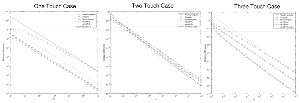
Figure 3: Relative differences for nonzero $\epsilon$ and $\epsilon=0$ for $L$ (weakly singular), $M$ (singular), and $L^{\prime}$ (hypersingular) integrals for
Left - One Touch: The lines show asymptotic dependences;
Center - Two Touch: Asymptotics of the hypersingular integral is used for the reference;
Right - Three Touch: Self-action analytical and asymptotic values are used for all integrals as reference.

The convergence in the one-touch case for integrals $L,M$, and $M^{\prime}$ is illustrated in Fig. 3 (left). In this case $\mathbf{y}_{10}=\left(0,0,0\right),$ $\mathbf{y}_{20}=\left(-1,0,0\right),$ $\mathbf{y}_{30}=\left(-1/2,0,\sqrt{3}/2\right)$. It is seen that all three integrals converge to their limiting values $L_{0}=0.182526568122379$, $M_{0}=0.055671118815334$, $M_{0}^{\prime}=0.063116905873345$ computed at $\epsilon=0$ at linear convergence rate. The constants for the linear convergence rates are computed using computed data for $\epsilon=10^{-7}$.

The convergence in the two-touch case for the same integrals is shown in Fig. 3 (center). Here we set $\mathbf{y}_{10}=\left(0,0,0\right),$ $\mathbf{y}_{20}=\left(1,0,0\right),$ $\mathbf{y}_{30}=\left(1/2,0,\sqrt{3}/2\right)$. The limiting values for the single and double layer potentials computed at $\epsilon=0$ are $L_{0}=0.415922738854561$ and $M_{0}=0.706739910625218$. We also obtained $M_{0}^{\prime}=M_{00}^{\prime}-H_{11}$, where $M_{00}^{\prime}=2.857471441252689$ is obtained at $\epsilon=0$ (see (5) under condition (93) for the common edge), and $H_{11}=2\ln(2/\epsilon)+2$ comes from (92) for the common edge length $l_{x1}=1$. Theoretically the convergence rates for $L$ and $M$ integrals are linear, while for $M^{\prime}$ this should be $\epsilon_{rel}\sim\epsilon/\ln(1/\epsilon)$. As in the previous case we determined the constants at some value of $\epsilon$ ($\epsilon=10^{-8}$) and plotted the curves on Fig. 3. Again, the consistency of the computed and theoretical rates is seen.

In the three-touch case illustrated in Fig. 3 (right) we have $\mathbf{y}_{j0}=\mathbf{x}_{j}$, $j=1,2,3$. Here we have the following limiting values, which can be computed straightforwardly (details are provided in the supplemental material), $L_{0}=\frac{3}{4}\ln 3$, and (94), (92), $M_{0}^{\prime}=M_{val}^{\prime}-3H_{11}$, $M_{val}=6\ln 3$. Here factor 3 in front of $H_{11}$ is due to the contribution described by (92) as we have three common edges in the three-touch case. It is remarkable that $M_{0}=0$, which is a true self-action value for the double layer, cannot be used for convergence study, as the double layer potential has a jump from $\pi$ on $S_{x}^{+}$ to $-\pi$ on $S_{x}^{-}$. Integration of this value over the area of the receiver triangle provides $M_{0}=\pi A_{y}=\pi\sqrt{3}/2$ as a limiting value as the receiver triangle approaches the source triangle from the side denoted as $S_{x}^{+}$ (from positive $z$ for the oriented triangle with the normal directed as $\mathbf{i}_{z}$). The expected convergence rates in this case are the same as in the two-touch case. We determined the constants by matching data at $\epsilon=10^{-8}$ and showed the approximations along with the calculated data in Fig. 3.

7.3 Comparison with [12], [17]

Salles [17] provides a matlab code to compute integrals calculated in [12] for cases #6 and #7 (in our notation). We executed this code for the cases from the “example of use” [17]. In these cases the vertices are $x_{1}=$ $\left(0,0,0\right)$, $x_{2}$ $=\left(0,1,0\right)$, $x_{3}$ $=$ $\left(1,0,0\right)$, $y_{1}=\left(0,0,h\right)$, $y_{2}=$ $\left(0,1,h\right)$, $y_{3}=\left(-1,0,h\right)$ for $L$ integrals, while the receiver triangle for $\mathbf{L}^{\prime}$ integral has vertices $y_{1}=\left(-2,0.5,0.01\right)$, $y_{2}=$ $\left(-1,1,0.01\right)$, $y_{3}=\left(-1,0,0.01\right).$ In Table 2 we provide outputs of [17] and ours in the same format.

Type	h	[12], [17]	This work	$\epsilon$
$L$	0	0.4154834934268203	0.4154834934268203	0
$L$	10-4	0.4154834087866362	0.4154834087866360	$2.2\cdot 10^{-16}$
$L$	10-3	0.4154773308369880	0.4154773308369882	$1.7\cdot 10^{-16}$
$L$	10-2	0.4150963397038615	0.4150963397038614	$1.1\cdot 10^{-16}$
$L$	10-1	0.3986731498732934	0.3986731498732936	$2.2\cdot 10^{-16}$
$L$	1	0.1994877345160992	0.1994877345160997	$5.6\cdot 10^{-16}$
$\mathbf{L}^{\prime}\cdot\mathbf{i}_{x}$	10-2	0.0937210251186380	0.0937210251186334	$4.6\cdot 10^{-15}$
$\mathbf{L}^{\prime}\cdot\mathbf{i}_{y}$	10-2	-0.0069668668015920	-0.0069668668016032	$1.1\cdot 10^{-14}$
$\mathbf{L}^{\prime}\cdot\mathbf{i}_{z}$	10-2	-0.0006289369951270	-0.0006289369951278	$7.8\cdot 10^{-16}$

Table 2: Comparison of the results of the present work with some data in literature [12], [17]. The absolute difference, $\epsilon$, between the results of the present study and [17] for $L$ is of the order of $10^{-16}$, i.e. consistent with double precision arithmetics. The difference for $\mathbf{L}^{\prime}$ is 1-2 orders of magnitude larger, but it is still small enough and can be explained by the round-off errors in summation of several terms of different magnitude.

8 Conclusion

This work shows that all integrals appearing in the Galerkin BEM with constant basis functions for the Laplace Green’s function can be evaluated analytically. However, one weakly singular integral formally can require 216 calls of the routine computing primitives. In practice, this can be reduced to 180 calls or lesser since some expansion coefficients are $s_{j0}$ are zero. Also, there exist some symmetries, which can be further investigated and used to improve efficiency. Furthermore, if simultaneous evaluation of single and double layer integrals and/or single layer derivatives is required a substantial amortization of computations occurs, as integrals in most cases can be computed simultaneously with little or no additional overhead.

For practical purposes the analytical integration can be employed for the nearfield integrals, while more efficient quadrature or expansion based [6] numerical integration can be applied for the far-field interactions. Nonetheless, the availability of the analytical methods to compute any kind of integrals is valuable for convergence studies and accurate evaluation of the order of the accuracy of the methods. In the future, the method can be extended to include linear and higher order basis function or include the Jacobians, which allow to account for curved panels, etc, as some work in this direction is already published (e.g., [18]).

The method can be extended to other than Laplace Green’s functions. Indeed, the recursive reduction process is the same independent of the kernel. All analytical challenges come only from construction of the PBF. A general expression for the PBF, however, is available (36). In the case, when not all four integrals can be computed straightforwardly, first, some reduction may be still available, and, second, some special functions can be introduced to make the PBF computable analytically or semi-analytically. Recursive layer potential integrals via dimensionality reduction for the Laplace and Helmholtz kernel for higher order elements in the context of collocation BEM is discussed in our recent work [9].

Appendix A Illustration of the algorithm applied to the computation of self-action integrals

A.1 Single layer potential

Let us consider the case of self-action integral, when triangles $S_{x}$ and $S_{y}$ coincide. To verify the general solution we can also derive analytical expressions for this case. Let us do this following the algorithm.

• Case definition. Equation (9) shows that in the case

  (95) $$\mathbf{X}_{0}=\mathbf{Y}_{0},\quad\mathbf{X}_{s}=\mathbf{Y}_{u},\quad\mathbf{X}_{t}=\mathbf{Y}_{v},$$

  while (46) provides for the 4D case

  (96) $$\mathbf{a}_{3}=\mathbf{-a}_{1}=-\mathbf{l}_{1},\quad\mathbf{a}_{4}=\mathbf{-a}_{2}=\mathbf{l}_{3},\quad\mathbf{e}_{4}=\mathbf{0},\quad U=I_{4}\left(\mathbf{l}_{1},-\mathbf{l}_{3},-\mathbf{l}_{1},\mathbf{l}_{3},\mathbf{0}\right).$$

  Here we used (13) where the subscript $x$ (or $y$) is removed, since $S_{x}$ and $S_{y}$ coincide.

• 4D to 3D reduction. Since $\mathbf{e}_{4}=\mathbf{0}$ we have from (16) and (18)

  (97) $$s_{10}=s_{20}=s_{30}=s_{40}=h_{4}=0.$$

  Relations (49) show then that only two 3D integrals contribute to the overall integral $U$

  (98) $$U=I_{32}+I_{35} =I_{3}\left(\mathbf{l}_{1},\mathbf{-l}_{3},\mathbf{-l}_{2},\mathbf{-l}_{1}\right)+I_{3}\left(-\mathbf{l}_{1},\mathbf{l}_{3},\mathbf{l}_{2},\mathbf{l}_{1}\right)=2I_{3}\left(\mathbf{l}_{1},\mathbf{-l}_{3},\mathbf{-l}_{2},\mathbf{-l}_{1}\right).$$

  Here, first, we used (51), (96), and (12) to express the arguments of $I_{3}$ integrals via $\mathbf{l}_{j}$ and, second, the fact that according the definition (14) and (15) the integrands depending on $R_{d}$ only (e.g. in (50)) do not change if we change the sign of all parameters to the opposite.

• 3D to 2D reduction. It is clear now, that $\mathbf{l}_{1}\in span\left(\mathbf{l}_{1},\mathbf{l}_{2},\mathbf{l}_{3}\right)$, and so $h_{3}=0$. Furthermore, since $\mathbf{e}_{3}=-\mathbf{l}_{1}$, the coefficients of expansion of $\mathbf{e}_{3}$ over vectors $\left(\mathbf{l}_{1},-\mathbf{l}_{2},-\mathbf{l}_{3}\right)$ can be selected as

  (99) $$s_{10}=-1,\quad s_{20}=0,\quad s_{30}=0.$$

  Relation (52) then shows that only two 2D integrals contribute to $I_{3}$, so

  (100) $$U =2I_{3}\left(\mathbf{l}_{1},\mathbf{-l}_{3},\mathbf{-l}_{2},\mathbf{-l}_{1}\right)=2\left(I_{22}+I_{24}\right)=2\left[I_{2}^{(s)}\left(\mathbf{-l}_{3},\mathbf{-l}_{2},-\mathbf{l}_{1}\right)+I_{2}^{(t)}\left(\mathbf{l}_{1},\mathbf{-l}_{3},\mathbf{l}_{3}\right)\right].$$

  where the arguments of the integrals are found using (54).

• 2D to 1D reduction. Again this clearly shows that since $\mathbf{l}_{1}=-\mathbf{l}_{2}-\mathbf{l}_{3}\in span\left(\mathbf{l}_{2},\mathbf{l}_{3}\right)$ and $\mathbf{l}_{2}\in span\left(\mathbf{l}_{1},\mathbf{l}_{2}\right)$ we have for both integrals in (100) $h_{2}=0$. Moreover,

  (101) $$\text{for }I_{2}^{(s)}:s_{10}=-1,\quad s_{20}=-1,\quad\text{for }I_{2}^{(t)}:s_{10}=0,\quad s_{20}=-1.$$

  From (100), (55), and (56) we obtain

  (102) $$U =2\left(I_{12}^{(s)}+I_{14}^{(s)}+I_{12}^{(t)}\right)=2\left[I_{1}\left(\mathbf{-l}_{2},-\mathbf{l}_{1}\right)+I_{1}\left(\mathbf{-l}_{3},-\mathbf{l}_{1}\right)+I_{1}\left(\mathbf{l}_{1},\mathbf{l}_{3}\right)\right]$$

  $$=2\sum_{j=1}^{3}I_{1}\left(\mathbf{l}_{j},\mathbf{e}_{1}^{(j)}\right),\quad\mathbf{e}_{1}^{(1)}=\mathbf{l}_{3},\quad\mathbf{e}_{1}^{(2)}=\mathbf{e}_{1}^{(3)}=\mathbf{l}_{1}.$$

  Here for convenience we rearranged summation and changed the signs of the arguments in two integrals (see the comment to (98)).

• Evaluation. First, we should determine the parallel and perpendicular projections of vectors $\mathbf{e}_{1}^{(j)}$. Generally, for projections we have (see Appendix)

  (103) $$\mathbf{e}_{1\|}^{(j)}=s_{10}^{(j)}\mathbf{l}_{j},\quad h_{1}^{(j)}=\left|\mathbf{e}_{1\bot}^{(j)}\right|=\left|\mathbf{e}_{1}^{(j)}-\mathbf{e}_{1\|}^{(j)}\right|,\quad s_{10}^{(j)}=\frac{\mathbf{e}_{1}^{(j)}\cdot\mathbf{l}_{j}}{l_{j}^{2}},\quad l_{j}=\left|\mathbf{l}_{j}\right|,\quad j=1,2,3.$$

  Since for all integrals $h_{2}=h_{3}=h_{4}=0$, we have from the first case of (45) and (57)

  (104) $$I_{1}\left(\mathbf{l}_{j},\mathbf{e}_{1}^{(j)}\right)=\left(1+s_{10}^{(j)}\right)F_{1}\left(P_{1}^{(j)}\left(1\right)\right)-s_{10}^{(j)}F_{1}\left(P_{1}^{(j)}\left(0\right)\right),$$

  $$P_{1}^{(j)}\left(s_{1}\right)=l_{j}\left|s_{1}+s_{10}^{(j)}\right|,\quad F_{1}\left(P_{1}^{(j)}\left(s_{1}\right)\right)=\frac{1}{12P_{1}^{(j)}}\ln\frac{\left(P_{1}^{(j)}+R_{1}^{(j)}\right)^{2}}{h_{1}^{\left(j\right)2}},$$

  $$R_{1}^{(j)}\left(s_{1}\right)=\sqrt{P_{1}^{(j)2}\left(s_{1}\right)+h_{1}^{\left(j\right)2}},\quad j=1,2,3.$$

• Simplification. Some simplifications can be obtained for the integrals listed above. We have

  (105) $$F_{1}\left(P_{1}^{(j)}\right)=\frac{1}{12P_{1}^{(j)}}\ln\frac{\left(R_{1}^{(j)}+P_{1}^{(j)}\right)^{2}}{R_{1}^{(j)2}-P_{1}^{(j)2}}=\frac{1}{12P_{1}^{(j)}}\ln\frac{R_{1}^{(j)}+P_{1}^{(j)}}{R_{1}^{(j)}-P_{1}^{(j)}}.$$

  This expression is invariant with respect to the sign of $P_{1}^{(j)}$, and so instead of $P_{1}^{(j)}\left(s_{1}\right)$ we can use the following signed function decorated by tilde

  (106) $$\widetilde{P}_{1}^{(j)}\left(s_{1}\right)=l_{j}\left(s_{1}+s_{10}^{(j)}\right),\quad F_{1}\left(P_{1}^{(j)}\right)=F_{1}\left(\widetilde{P}_{1}^{(j)}\right)=\frac{1}{12\widetilde{P}_{1}^{(j)}}\ln\frac{R_{1}^{(j)}+\widetilde{P}_{1}^{(j)}}{R_{1}^{(j)}-\widetilde{P}_{1}^{(j)}}.$$

  Hence, integral in (104) turns into

  (107) $$I_{1}\left(\mathbf{l}_{j},\mathbf{e}_{1}^{(j)}\right)= \left(1+s_{10}^{(j)}\right)F_{1}\left(\widetilde{P}_{1}^{(j)}\left(1\right)\right)-s_{10}^{(j)}F_{1}\left(\widetilde{P}_{1}^{(j)}\left(0\right)\right)$$

  $$= \frac{1}{12l_{j}}\ln\frac{R_{1}^{(j)}\left(1\right)+\widetilde{P}_{1}^{(j)}\left(1\right)}{R_{1}^{(j)}\left(1\right)-\widetilde{P}_{1}^{(j)}\left(1\right)}\frac{R_{1}^{(j)}\left(0\right)-\widetilde{P}_{1}^{(j)}\left(0\right)}{R_{1}^{(j)}\left(0\right)+\widetilde{P}_{1}^{(j)}\left(0\right)}.$$

  It follows from (102) and (103) that

  (108) $$s_{10}^{(1)}=\frac{\mathbf{l}_{1}\cdot\mathbf{l}_{3}}{l_{1}^{2}}=\frac{l_{2}^{2}-l_{1}^{2}-l_{3}^{2}}{2l_{1}^{2}},\quad s_{10}^{(2)}=\frac{\mathbf{l}_{1}\cdot\mathbf{l}_{2}}{l_{2}^{2}}=\frac{l_{3}^{2}-l_{1}^{2}-l_{2}^{2}}{2l_{2}^{2}},\quad s_{10}^{(3)}=\frac{\mathbf{l}_{1}\cdot\mathbf{l}_{3}}{l_{3}^{2}}=\frac{l_{2}^{2}-l_{1}^{2}-l_{3}^{2}}{2l_{3}^{2}},$$

  where we got rid of scalar products using the cosine theorem for the triangle (or $\left|\mathbf{l}_{1}+\mathbf{l}_{2}\right|^{2}=\left|\mathbf{l}_{3}\right|^{2}$)

  (109) $$l_{1}^{2}+2\mathbf{l}_{1}\cdot\mathbf{l}_{2}+l_{2}^{2}=l_{3}^{2},\quad\mathbf{l}_{1}\cdot\mathbf{l}_{2}=\frac{l_{3}^{2}-l_{1}^{2}-l_{2}^{2}}{2}.$$

  Furthermore, we have the following expressions for functions $\widetilde{P}_{1}^{(j)}$ and $R^{(j)}$

  (110) $$R_{1}^{(1)}\left(0\right)= l_{3},\quad R_{1}^{(2)}\left(0\right)=l_{1},\quad R_{1}^{(3)}\left(0\right)=l_{1},\quad R_{1}^{(1)}\left(1\right)=l_{2},\quad R_{1}^{(2)}\left(1\right)=l_{3},$$

  $$R_{1}^{(3)}\left(1\right) =l_{2},\quad\widetilde{P}_{1}^{(j)}\left(0\right)=l_{j}s_{j0}^{(1)},\quad\widetilde{P}_{1}^{(j)}\left(1\right)=l_{j}\left(1+s_{10}^{(j)}\right),\quad j=1,2,3.\quad$$

  Substituting these into expressions for integrals (107) and simplifying, we obtain

  (111) $$I_{1}\left(\mathbf{l}_{j},\mathbf{e}_{1}^{(j)}\right)=\frac{1}{6l_{j}}\ln\frac{l_{1}+l_{2}+l_{3}}{l_{1}+l_{2}+l_{3}-2l_{j}},\quad j=1,2,3,$$

  The final expressions (102) and (11), therefore, can be written in the form

  (112) $$L=4A^{2}U,\quad U=\frac{1}{3}\sum_{j=1}^{3}\frac{1}{l_{j}}\ln\frac{p}{p-l_{j}},\quad p=\frac{1}{2}\sum_{j=1}^{3}l_{j},$$

  where $p$ is the half of the perimeter and $A$ is the area of triangle $S_{x}.$ This is consistent with the expression derived in [3] and simplified in [20] (the expression under logs there can be slightly simplified to obtain (112; also the modulus under log can be removed, since the expression is always positive due to the triangle inequality $p>l_{j},$ $j=1,2,3$).

A.2 Gradient of single layer and double layer potential

Similarly to the single layer case we can consider for illustration computation of the self-action integral. As it is mentioned in this case we have $M=0$. This case is characterized by $h_{4}=h_{3}=h_{2}=0$. So, based on $\mathbf{a}_{1},...,\mathbf{a}_{4},\mathbf{e}_{4}$ from (96) we can determine parameters of 3D integrals, which are

(113) $$F_{1}=6l_{1}AI_{3}\!\left(\mathbf{-l}_{1},\mathbf{l}_{3},\mathbf{l}_{1},\mathbf{0}\right),\quad\!\!\!F_{2}=6l_{2}AI_{3}\!\left(\mathbf{-l}_{1},\mathbf{l}_{3},\mathbf{l}_{2},\mathbf{l}_{1}\right),\quad\!\!\!F_{3}=6l_{3}AI_{3}\!\left(\mathbf{-l}_{1},\mathbf{l}_{3},\mathbf{-l}_{3},\mathbf{0}\right),$$

where we used relation (66) expressing $\widehat{I}_{3}$ via $I_{3}$ and removed subscript $x$ as $S_{x}$ and $S_{y}$ coincide. Following the same procedure as (99)-(112) we can find that

(114) $$F_{i}=\frac{3l_{i}}{4A}L,\quad i=1,2,3,$$

where $L$ is from (112). Final summation then yields

(115) $$\mathbf{F}=\sum_{i=1}^{3}\mathbf{n}_{ci}F_{i}=-\mathbf{n\times}\sum_{i=1}^{3}\frac{\mathbf{l}_{i}}{l_{i}}F_{i}=\frac{3L}{4A}\mathbf{n}\times\sum_{i=1}^{3}\mathbf{l}_{i}=\mathbf{0.}$$

Appendix B Method for identifying the parameters

Given some vector $\mathbf{e}_{d}\in\mathbb{R}^{3}$ and a set of vectors $\left\{\mathbf{a}_{1},...,\mathbf{a}_{d}\right\}$, $\mathbf{a}_{j}\in\mathbb{R}^{3}$, $\mathbf{a}_{j}\neq 0,$ $j=1,...,d,$ we need to determine the perpendicular and parallel components $\mathbf{e}_{d\bot}$ and $\mathbf{e}_{d||}$, $\mathbf{e}_{d}=\mathbf{e}_{d||}+\mathbf{e}_{d\perp}$, such that $\mathbf{e}_{d||}\in span\left(\mathbf{a}_{1},...,\mathbf{a}_{d}\right)$, while $\mathbf{e}_{d\perp}\cdot\mathbf{a}_{j}=0$. Moreover, we need to find the coefficients of expansion $s_{10},...,s_{d0}$ for the parallel component $\mathbf{e}_{d||}=s_{10}\mathbf{a}_{1}+...+s_{d0}\mathbf{a}_{d}$. $h_{d}$ is defined as the norm of vector $\mathbf{e}_{d\perp}$. We briefly describe how to do this using Gram-Schmidt orthogonalization.

The original Gram-Schmidt algorithm is designed for orthogonalization of a linearly independent vector set, while here some vectors $\mathbf{a}_{1},...,\mathbf{a}_{d}$ are linearly dependent. So, the proposed procedure consist of two steps: orthogonalization, and, determination of the expansion coefficients.

B.1 Orthogonalization

The standard Gram-Schmidt process is given as

(116) $$\mathbf{u}_{1}=\mathbf{a}_{1},\quad\mathbf{u}_{i}=\mathbf{a}_{i}-\sum_{k=1}^{i-1}c_{ki}\mathbf{u}_{k},\quad i=2,...,d,\quad c_{ki}=\frac{\mathbf{u}_{k}\cdot\mathbf{a}_{i}}{\left|\mathbf{u}_{k}\right|^{2}},$$

where $\left\{\mathbf{u}_{1},...,\mathbf{u}_{d}\right\}$ is the orthogonal set, such as $span\left(\mathbf{u}_{1},...,\mathbf{u}_{d}\right)=span\left(\mathbf{a}_{1},...,\mathbf{a}_{d}\right)$ and $c_{ki}\mathbf{u}_{k}$ is the projection of $\mathbf{a}$ on $\mathbf{u}_{k}$. As the steps $i=2,...,d$ are applied recursively all $\left\{\mathbf{u}_{1},...,\mathbf{u}_{d}\right\}$ can be obtained for the linearly independent set $\left\{\mathbf{a}_{1},...,\mathbf{a}_{d}\right\}$. In case if $\mathbf{a}_{j}$ depends linearly on $\mathbf{a}_{1},...,\mathbf{a}_{j-1}$(i.e., $\mathbf{a}_{j}\in span\left\{\mathbf{a}_{1},...,\mathbf{a}_{j-1}\right\}$) the process produces $\mathbf{u}_{j}=\mathbf{0}$ and cannot be continued as represented by (116), since $\left|\mathbf{u}_{j}\right|=0$. An easy way to modify the process which can pass through linearly dependent vectors is to redefine the projection coefficients as

(117) $$c_{ki}=\frac{\mathbf{u}_{k}\cdot\mathbf{a}_{i}}{u_{k}^{2}},\quad u_{k}^{2}=\left\{\begin{array}[]{c}\left|\mathbf{u}_{k}\right|^{2},\quad\left|\mathbf{u}_{k}\right|\neq 0\\ 1,\quad\left|\mathbf{u}_{k}\right|=0\end{array}\right.,\quad i,k=1,...,d$$

The process (116) produces the orthogonal set $\left\{\mathbf{u}_{1},...,\mathbf{u}_{d}\right\}$ with $\mathbf{u}_{j}$ $=\mathbf{0}$ in place of $\mathbf{a}_{j}\in span\left\{\mathbf{a}_{1},...,\mathbf{a}_{j-1}\right\}.$

B.2 Expansion coefficients

We can now expand all vectors $\mathbf{a}_{1},...,\mathbf{a}_{d}$ over the set $\left\{\mathbf{u}_{1},...,\mathbf{u}_{d}\right\}$ as

(118) $$\mathbf{a}_{i}=\sum_{k=1}^{i}c_{ki}\mathbf{u}_{k},\quad i=1,...,d,$$

considering the expansion

(119) $$\mathbf{e}_{d}=\sum_{i=1}^{d}s_{i0}\mathbf{a}_{i}+\mathbf{e}_{d\bot}=\sum_{i=1}^{d}s_{i0}\sum_{k=1}^{i}c_{ki}\mathbf{u}_{k}+\mathbf{e}_{d\bot}.$$

Taking the scalar product of $\mathbf{e}_{d}$ and $\mathbf{u}_{j}$ we obtain

(120) $$\sum_{i=1}^{d}A_{ji}s_{i0}=b_{j},\quad A_{ji}=c_{ji}\left|\mathbf{u}_{j}\right|^{2},\quad b_{j}=\mathbf{u}_{j}\cdot\mathbf{e}_{d},\quad j=1,...,d.$$

This is a linear system for unknowns $s_{i0}$ with the upper triangular matrix with entries $A_{ji}$ and the right hand side vector with components $b_{j}$. It can be solved recursively. For the $j$th row corresponding to $\mathbf{u}_{j}=\mathbf{0}$ we have $A_{ji}=0$ and $b_{j}=0$;  so, one should set $s_{j0}=0$. The solution is then

(121) $$s_{j0}=\left\{\begin{array}[]{c}\frac{1}{A_{jj}}\left(b_{j}-\sum_{i=j+1}^{d}A_{ji}s_{i0}\right),\quad A_{jj}\neq 0\\ 0,\quad A_{jj}=0\end{array}\right.,\quad j=d,d-1,...,1.$$

As soon as all $s_{i0}$ are determined, parameter $h_{d}$ can be found from

(122) $$h_{d}=\left|\mathbf{e}_{d\bot}\right|=\left|\mathbf{e}_{d}-\sum_{i=1}^{d}s_{i0}\mathbf{a}_{i}\right|.$$

References

- [1] R. Adelman, N. A. Gumerov, and R. Duraiswami, Computation of Galerkin double surface integrals in the 3-D boundary element method, IEEE Trans. Ant. Propagat., 64 (2016), pp. 2389–2400.
- [2] J. D’Elía, L. Battaglia, A. Cardona, and M. Storti, Full numerical quadrature of weakly singular double surface integrals in Galerkin boundary element methods, Int. J. Num. Meth. Biomed. Engg., 27 (2011), pp. 314–334.
- [3] T. F. Eibert and V. Hansen, On the calculation of potential integrals for linear source distributions on triangular domains, IEEE Trans. Ant. Propagat., 43 (1995), pp. 1499–1502.
- [4] L. Gray and T. Kaplan, 3D Galerkin integration without Stokes’ theorem, Engg. Anal. Boundary Elem., 25 (2001), pp. 289–295.
- [5] N. A. Gumerov and R. Duraiswami, Analytical computation of boundary integrals for the Helmholtz equation in three dimensions, arXiv:2103.17196, (2021).
- [6] N. A. Gumerov and R. Duraiswami, Efficient Fast Multipole Accelerated Boundary Elements via Recursive Computation of Multipole Expansions of Integrals, arXiv preprint arXiv:2107.10942, (2021).
- [7] R. Harrington, Field Computation by Moment Methods, New York: Macmillan, 1983.
- [8] J. L. Hess and A. O. Smith, Calculation of potential flow about arbitrary bodies, Progress in Aerospace Sciences, 8 (1967), pp. 1–138.
- [9] S. Kaneko, N. A. Gumerov, and R. Duraiswami, Recursive Analytical Quadrature of Laplace and Helmholtz Layer Potentials in , arXiv preprint arXiv:2302.02196, (2023).
- [10] G. A. Korn and T. M. Korn, Mathematical handbook for scientists and engineers: definitions, theorems, and formulas for reference and review, Courier Corporation, 2000.
- [11] M. Lenoir, Influence coefficients for variational integral equations, Comptes Rendus Mathematique, 343 (2006), pp. 561–564.
- [12] M. Lenoir and N. Salles, Evaluation of 3-D singular and nearly singular integrals in Galerkin BEM for thin layers, SIAM Journal on Scientific Computing, 34 (2012), pp. A3057–A3078.
- [13] M. Lenoir and N. Salles, Exact evaluation of singular and near-singular integrals in Galerkin BEM, Proceedings of ECCOMAS2012, (2012), pp. 1–20.
- [14] S. Oueslati, I. Balloumi, C. Daveau, and A. Khelifi, Analytical method for the evaluation of singular integrals arising from boundary element method in electromagnetism, Int. J. Num. Mod.: Electronic Networks, Devices Fields, 34 (2021), p. e2792.
- [15] A. G. Polimeridis, J. M. Tamayo, J. M. Rius, and J. R. Mosig, Fast and accurate computation of hypersingular integrals in Galerkin surface integral equation formulations via the direct evaluation method,IEEE Trans. Ant. Propagat., 59 (2011), pp. 2329–2340.
- [16] D. Rosen and D. E. Cormack, Singular and near singular integrals in the BEM: A global approach, SIAM Journal on Applied Mathematics, 53 (1993), pp. 340–357.
- [17] N. Salles, Matlab implementation of the formulas. http://www.nsalles.org/codesisc/.
- [18] N. Salles, Calculation of singularities in variational integral equations methods, HAL, (2013).
- [19] A. Salvadori, Analytical integrations of hypersingular kernel in 3D BEM problems, Computer methods in applied mechanics and engineering, 190 (2001), pp. 3957–3975.
- [20] D. Sievers, T. F. Eibert, and V. Hansen, Correction to “On the calculation of potential integrals for linear source distributions on triangular domains”, IEEE Transactions on Antennas and Propagation, 53 (2005), pp. 3113–3113.
- [21] N. G. Warncke, I. Ciotir, A. Tonnoir, Z. Lambert, and C. Gout, Analytical approach to Galerkin BEMs on polyhedral surfaces, The SMAI journal of computational mathematics, 5 (2019), pp. 27–46.