Exact Inference in High-order Structured Prediction
Abstract
In this paper, we study the problem of inference in high-order structured prediction tasks. In the context of Markov random fields, the goal of a high-order inference task is to maximize a score function on the space of labels, and the score function can be decomposed into sum of unary and high-order potentials. We apply a generative model approach to study the problem of high-order inference, and provide a two-stage convex optimization algorithm for exact label recovery. We also provide a new class of hypergraph structural properties related to hyperedge expansion that drives the success in general high-order inference problems. Finally, we connect the performance of our algorithm and the hyperedge expansion property using a novel hypergraph Cheeger-type inequality.
1 Introduction
Structured prediction has been widely used in various machine learning fields in the past years, including applications like social network analysis, computer vision, molecular biology, natural language processing (NLP), among others. A common objective in these tasks is assigning / recovering labels, that is, given some possibly noisy observation, the goal is to output a group label for each entity in the task. In social network analysis, this could be detecting communities based on user profiles and preferences (Kelley et al., 2012). In computer vision, researchers want the AI to decide whether a pixel is in the foreground or background (Nowozin et al., 2011). In biology, it is sometimes desirable to cluster molecules by structural similarity (Nugent and Meila, 2010). In NLP, part-of-speech tagging is probably one of the most well-known structured prediction task (Weiss and Taskar, 2010).
From a methodological point of view, a standard approach in the structured prediction tasks above, is to recover the global structure by exploiting many local structures. Take social networks as an example. A widely used assumption in social network analysis is affinity — users with similar profiles and preferences are more likely to become friends. Intuitively, a structured prediction algorithm tends to assign two users the same label, if they have a higher affinity score. Similarly, the same idea can be motivated in the context of Markov random fields (MRFs). Assume all entities form an undirected graph , structured prediction can be viewed as the task of solving the following inference problem (Bello and Honorio, 2019):
| (1) |
where is the space of labels, is the score of assigning label to node , and is the score of assigning labels and to neighboring nodes and . In the MRF and inference literature, the two terms in (1) are often referred to as unary and pairwise potentials, respectively. The inference formulation above allows one to recover the global structure, by finding a configuration that maximizes the summation of unary and pairwise local scores.
However, entities in many real-world problems could interact beyond the pairwise fashion. Take the social network example again, but this time let us focus on the academia co-authorship network: many published papers are written by more than two authors (Liu et al., 2005). Such high-order interactions cannot be captured by pairwise structures. Geometrically, the co-authorship network can no longer be represented by a graph. As a result, the introduction of hypergraphs is necessary to model high-order structured prediction problems.
In this paper, we study the problem of high-order structured prediction, in which instead of using pairwise potentials, high-order potentials are considered. Using the MRF formulation, we are interested in inference problems of the following form:
| (2) |
where is the order of the inference problem as well as the hypergraph (each hyperedge connects vertices), and is the score of assigning labels through to neighboring nodes through connected by hyperedge .
1.1 Inference as a Recovery Task
Structured prediction and inference problems with unary and pairwise potentials in the form of (1) have been studied in prior literature. Globerson et al. (2015) introduced the problem of label recovery in the case of two-dimensional grid lattices, and analyzed the conditions for approximate inference. Along the same line of work, Foster et al. (2018) generalized the model by allowing tree decompositions. Another flavor is the problem of exact inference, for which Bello and Honorio (2019) proposed a convex semidefinite programming (SDP) approach. In these works, the problem of label recovery is motivated by a generative model, which assumes the existence of a ground truth label vector , and generates (possibly noisy) unary and pairwise observations based on label interactions.
Unfortunately, little is known for structured prediction with high-order potentials and hypergraphs. In recent years, there have been various attempts to generalize some graph properties (including hypergraph Laplacian, Rayleigh quotient, hyperedge expansion, Cheeger constant, among others) to hypergraphs (Li and Milenkovic, 2018; Mulas, 2021; Yoshida, 2019; Chan et al., 2018; Chen et al., 2017; Chang et al., 2020). However, it took a long time for us to find out that due to the nature of structured prediction tasks, the hypergraph definitions must fulfill certain properties, and none of the definitions in the aforementioned works fulfill those. This makes it challenging to design hypergraph-based label recovery algorithms. Furthermore, none of the aforementioned works provide guarantees of either approximate or exact inference.
In this work, we apply a generative model approach to study the problem of high-order inference. We analyze the task of label recovery, and answer the following question:
Problem 1 (Label Recovery).
Is there any algorithm that takes noisy unary and high-order local observation as the input, and correctly recovers the underlying true labels?
1.2 Inference and Structural Properties
In the MRF inference literature, a central and longtime discussion focuses on inference solvability versus certain structural properties of the problem.
To see this, we first revisit various classes of structural properties in pairwise inference problems (i.e., in the form of (1)). Chandrasekaran et al. (2012) studied treewidth in graphs as a structural property, and showed that graphs with low treewidths are solvable. Schraudolph and Kamenetsky (2008) demonstrated that planar graphs can be solved. Boykov and Veksler (2006) analyzed graphs with binary labels and sub-modular pairwise potentials. Bello and Honorio (2019) showed that inference with graphs that are “good” expanders, or “bad” expanders plus an Erdos-Renyi random graph, can be achieved. It is worth highlighting that the structural properties above are not directly comparable or reducible. Instead, they characterize the difficulty of an inference problem from different angles, or in other words, for different classes of graphs.
Similar discussions about inference versus structural properties exist in high-order MRF inference literature. For example, Komodakis and Paragios (2009) investigated hypergraphs fulfilling the property of one sub-hypergraph per clique, and proved that high-order MRF inference can be achieved through solving linear programs (LPs). Fix et al. (2014) studied inference in hypergraphs with the property of local completeness. Gallagher et al. (2011) analyzed the performance of high-order MRF inference through order reduction versus the number of non-submodular edges. However, these works do not provide theoretical guarantees of either approximate or exact inference.
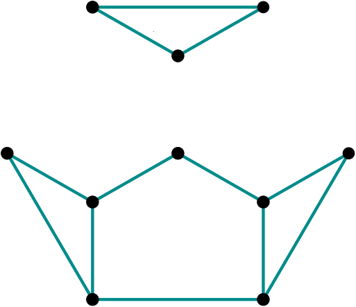
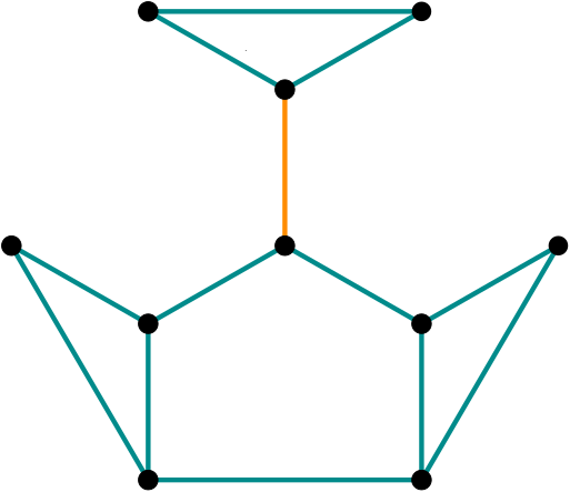
In this paper, we provide a new class of hypergraph structural properties by analyzing hyperedge expansion. In order to get some intuition, let us consider a social network with two disconnected sub-networks. With an ideal algorithm, we may recover the user communities in subnet 1 and the those in subnet 2, but since there is no interaction between the two subnets at all, we will not be able to infer the global community structure (e.g., the relationship between the recovered communities in subnet 1 and subnet 2). A less extreme case is networks with “bottlenecks,” i.e., removing these bottleneck edges will disconnect the network. For similar reasons, one can imagine that inference in networks with bottlenecks can be hard if noise is present. See Figure 1 for an illustration. In pairwise graphs (-graphs), such connectivity / bottleneck property can be characterized by the edge expansion (i.e., the Cheeger constant) of the graph. Characterizing similar expansion properties in high-order hypergraphs poses a challenge, especially if one wants to relate such topological properties to the conditions of exact inference.
Problem 2 (Structural Property).
Under what topological conditions will our label recovery algorithm work correctly with high probability?
Summary of our contribution. Our work is highly theoretical. We provide a series of novel definitions and results in this paper:
-
•
We provide a new class of hypergraph structural properties for high-order inference problems. We derive a novel Cheeger-type inequality, which relates the tensor spectral gap of a hypergraph Laplacian to a Cheeger-type hypergraph expansion property. These hypergraph results are not only limited to the scope of the model in this paper, but also can be helpful to researchers working on high-order inference problems.
-
•
We propose a two-stage approach to solve the problem of high-order structured prediction. We formulate the label recovery problem as a high-order combinatorial optimization problem, and further relax it to a novel convex conic form optimization problem.
-
•
We carefully analyze the Karush–Kuhn–Tucker (KKT) conditions of the conic form optimization problem, and derive the sufficient statistical and topological conditions for exact inference. Our KKT analysis guarantees the solution to be optimal with a high probability, as long as the conditions are fulfilled.
2 Preliminaries
In this section, we formally define the high-order exact inference problem and introduce the notations that will be used throughout the paper.
We use lowercase font (e.g., ) to denote scalars and vectors, and uppercase font (e.g., ) to denote tensors. We denote the set of real numbers by .
For any natural number , we use to denote the set .
We use to denote the all-ones vector.
For clarity we use superscripts to denote the -th object in a sequence of objects, and subscripts to denote the -th entry. We use to denote the Hadamard product, and to denote the outer product. Let be a sequence of vectors of dimension . Then is a tensor of order and dimension (or equivalently, of shape ), such that
2.1 Tensor Definitions
Let be an -th order, -dimensional real tensor. Throughout the paper, we limit our discussion to for clarity of exposition. While other even orders () are possible and a similar analysis will follow, the hypergraph definitions will be involving many more terms and the paper will be less readable. See Remark 3.17 for discussion.
A symmetric tensor is invariant under any permutation of the indices. In other words, is symmetric if for any permutation , we have .
We define the inner product of two tensors , of the same shape as . We define the tensor Frobenius norm as .
A symmetric tensor is positive semidefinite (PSD), if for all , we have . We use to denote the convex cone of all -order, -dimensional PSD tensors.
The dual cone of is the Caratheodory tensor cone , which is defined as . In other words, every tensor in is the summation of at most rank-one tensors. and are dual to each other (Ke and Honorio, 2022).
For any tensor , we define its minimum tensor eigenvalue (or equivalently ) using a variational characterization, such that . Similarly we define its second minimum tensor eigenvalue as , where is the eigenvector corresponding to .
We denote as the index set of -tuples in the shape of , for any permutation and . Intuitively, in every tuple of , every index repeats an even number of times. We use to denote the set . In other words, is the complement of , subtracting cases with all unique indices.
2.2 High-order Inference Task
We consider the task of predicting a set of vertex labels , where , from a set of observations and . and are noisy observations generated from some underlying -uniform hypergraph . In particular, is the set of vertices (nodes) with , and is the set of hyperedges.
For every possible -vertex tuple , if , the hyperedge observation (and all corresponding symmetric entries ) is sampled to be with probability , and with probability independently. If , is set to .
For every node , the node observation is sampled to be with probability , and with probability independently.
We now summarize the generative model.
Definition 2.1 (High-order Structured Prediction with Partial Observation).
Unknown: True node labeling vector . Observation: Partial and noisy hyperedge observation tensor . Noisy node label observation vector . Task: Infer and recover the correct node labeling vector from the observation and .
3 Hypergraph Structural Properties and Cheeger-type Inequality
In this section, we introduce a series of novel Cheeger-type analysis for hypergraphs. This allows us to characterize the spectral gap of a hypergraph Laplacian, via the topological hyperedge expansion of the graph itself. Hypergraph theorems in this section are general, and are not limited to the specific model covered in our inference task. To the best of our knowledge, the following high-order definitions and results are novel. All missing proofs of the lemmas and theorems can be found in Appendix A.
3.1 Hypergraph Topology
We first introduce the necessary hypergraph topological definitions.
Definition 3.1 (Induced Hypervertices).
Given an -uniform hypergraph , we use
to denote the set of induced hypervertices. We denote its cardinality by .
Definition 3.2 (Boundary of a Hypervertex Set).
For any hypervertex set , we denote its boundary set as
Note that is a set of -th order hyperedges and non-edges.
Definition 3.3 (Hyperedge Expansion of a Hypervertex Set).
For any hypervertex set , we denote the hyperedge expansion of the set as
Definition 3.4 (Hyperedge Expansion of a Hypergraph).
Given an -uniform hypergraph with induced hypervertices , we denote the hyperedge expansion of the hypergraph as
We also call the Cheeger constant of the hypergraph.
3.2 Hypergraph Laplacian
In this section, we introduce our hypergraph Laplacian related definitions.
Definition 3.5 (-function).
is a function defined as
Definition 3.6 (Hypergraph Laplacian).
Given an -uniform hypergraph , we use to denote its Laplacian tensor, which fulfills
Definition 3.7 (Rayleigh Quotient).
For any hypergraph Laplacian and non-zero vector , the Rayleigh quotient is defined as
Definition 3.8 (Signed Laplacian Tensor).
Given an -uniform hypergraph with a sign vector , we use to denote its signed Laplacian tensor, which fulfills
Remark 3.9.
The hypergraph Laplacian tensor can be viewed as a signed Laplacian tensor , by taking .
Here we provide some important properties of hypergraph Laplacians and Rayleigh quotients.
Lemma 3.10 (Laplacian Eigenpair).
For any hypergraph Laplacian , is an eigenvector of with a minimum eigenvalue of . Similarly, for any signed hypergraph Laplacian , is an eigenvector of with an eigenvalue of .
Proof of Lemma 3.10.
Lemma 3.11 (Invariant under Scaling).
For any non-zero , we have
Proof of Lemma 3.11.
∎
Lemma 3.12 (Invariant under Scaling).
For any and , , we have
Proof of Lemma 3.12.
Note that
where the inequality follows from the fact that
∎
Lemma 3.13 (Signed Rayleigh Quotient Lower Bound).
For any hypergraph with Laplacian and signed Laplacian , and for any and , , we have
Lemma 3.14 (Existance of Degree Tensor).
For any hypergraph Laplacian , let denote the corresponding symmetric adjacency tensor, such that if and only if . Then, there exists a high-order degree tensor fulfilling: 1) if are all different, and 2) for every vector .
3.3 High-order Cheeger-type Inequality
Here, we connect the previous two sections and provide our novel high-order Cheeger-type inequality.
Theorem 3.15 (High-order Cheeger-type Inequality).
For any -uniform hypergraph with Laplacian , we have
Remark 3.16.
Here we would like to discuss our choice of hypergraph Laplacian as well as the related high-order definitions. Despite the fact that there have been multiple works trying to generalize some graph properties (including hypergraph Laplacian, Rayleigh quotient, hyperedge expansion, Cheeger constant, among others) to hypergraphs (Li and Milenkovic, 2018; Mulas, 2021; Yoshida, 2019; Chan et al., 2018; Chen et al., 2017; Chang et al., 2020), we want to highlight that none above fulfill the requirement of our high-order inference tasks.
To obtain a set of hypergraph definitions that are useful for our inference task, we need to fulfill all the lemmas in this section. In particular, here are the necessary conditions:
- •
-
•
To fulfill Lemma 3.12, the -function (Definition 3.5) and the norm in the denominator of the Rayleigh quotient (Definition 3.7) must have the same power. Additionally, the summation of coefficients of the terms in the parenthesis in the -function (Definition 3.5) must be . Combining with the last condition, it requires the number of plus and minus terms to be equal.
- •
-
•
To fulfill Lemma 3.10, the Rayleigh quotient must achieve minimum with .
At this point it should be clear that we cannot simply use some arbitrary definition from the prior literature. Our hypergraph definitions are carefully constructed and chosen, to fulfill all the necessary conditions above.
Remark 3.17.
Regarding the choice of order , note that if is odd, the task of label recovery will not be feasible in the current formulation, since the Rayleigh quotient will be unbounded below (instead of a minimum ). From Remark 3.16 it can be noticed that if we keep the current definition of -functions, the only possible ’s are The definition of -functions can be generalized for other even orders, such that for every -tuple , we take the average of many -power terms by iterating through the permutation of all possible signs. For clarity of exposition we keep the current simpler definition, and focus on the case of
4 Exact Recovery of True Labels
In this section, we present an inference algorithm, which recovers the underlying true labels in our model. To do so, we take a two stage approach. In the first stage we only utilize the hyperedge information observed from , and this allows us to narrow down our solution space to two possible solutions. In the second stage, with the help of the node information observed from , we are able to infer the correct labeling of the nodes.
4.1 Stage One: Inference up to Permutation
We start by considering the following combinatorial problem
| (3) |
The issue with this optimization formulation is that the problem is not convex, which makes the analysis hard and intractable. Instead, we consider the following relaxed version
| (4) |
Alternatively, we represent the last two constraints as , and . Recall that is the convex cone of rank-one tensors. The motivation is that we are using a rank-one tensor instead of the outer product , so that the problem becomes convex in the objective function and the constraints. We have because the product of ’s is either or , and we have because if every repeats an even number of times, we know the product must be .
It remains to prove correctness of program (4). We are interested in identifying the regime, in which (4) returns the exact rank-one tensor solution . We now present our main theorem on inference. The proof can be found in Appendix B.
Theorem 4.1 (Inference from Hyperedge Observation).
For an -order structured prediction model with underlying hypergraph and hyperedge observation , the rank-one tensor solution can be recovered from the convex optimization program (4) with probability at least , where
| (5) |
Remark 4.2.
A natural question to ask is, under what topological and statistical conditions can we obtain a high probability guarantee from Theorem 4.1. An observation is that if the Cheeger constant of the underlying hypergraph is large, or the noise level is small, recovery is more likely to succeed. In Section 5, we analyze at some interesting classes of hypergraphs with good expansion property (large Cheeger constant), so that high probability recovery can be guaranteed.
4.2 Stage Two: Exact Inference
In the previous section, we established the high probability inference guarantee for the rank-one tensor solution . By taking a factorization step, we know either or is the correct label vector. In this section, our goal is to decide the correct labeling using the node observation .
Theorem 4.3.
Let . The correct label vector can be recovered from program
| (6) |
with probability at least , where
| (7) |
Proof of Theorem 4.3.
Applying Hoeffding’s inequality, we obtain that
∎
Corollary 4.4.
Remark 4.5.
Given , we observe that as long as , we know (an exponential decay). As a result, whether one can obtain a high probability guarantee in the shape of depends only on the order of , that is, the topological structure of the underlying hypergraph. In Section 5, we investigate hypergraphs with good expansion properties, that allow us to achieve a high probability guarantee of exact inference.
5 Examples of Hypergraphs with Good Expansion Property
In this section, we consider some example classes of hypergraphs with good expansion property, and demonstrate that they lead to high probability guarantees in our exact inference algorithm.
We first analyze complete hypergraphs.
Definition 5.1 (Complete Hypergraphs).
An -uniform hypergraph is complete, if for every -vertex tuple , we have .
Proposition 5.2 (Expansion Property of Complete Hypergraphs).
For any complete hypergraph , we have
Proof.
Corollary 5.3 (Exact Inference in Complete Hypergraphs).
Let be a complete hypergraph. Assume . Then exact inference can be achieved using the proposed two-stage approach with probability tending to with a sufficiently large .
Proof.
Note that for complete hypergraphs, we have
Substituting into (8), as long as is greater than some constant , we have
∎
Next, we focus on the case of regular expanders.
Definition 5.4 (-regular Expander).
An -uniform hypergraph is a -regular expander hypergraph with constant , if for any induced hypervertex set with , we have
Proposition 5.5 (Expander Hypergraphs).
For any -regular expander hypergraph with constant , we have
Proof.
Corollary 5.6 (Exact Inference in Expander Hypergraphs).
Let be a -regular expander hypergraph with constant . Assume . Then exact inference can be achieved using the proposed two-stage approach with probability tending to with a sufficiently large , if
Proof.
5.1 Simulation Results
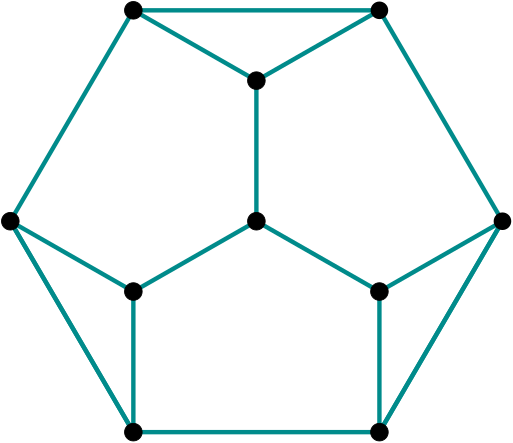
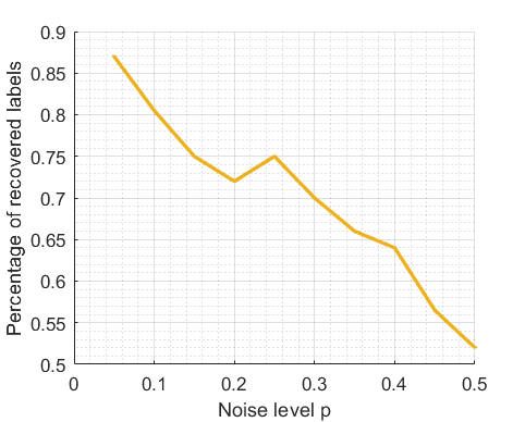
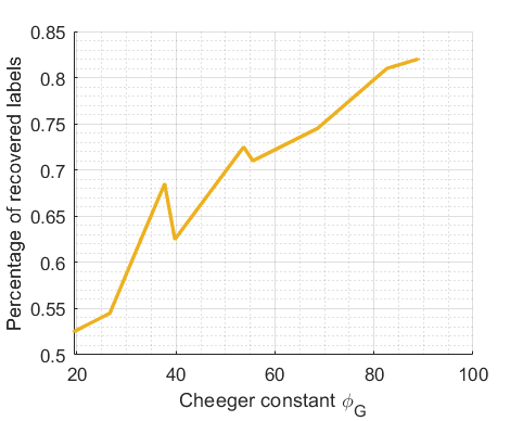
We test the proposed method on a hypergraph with order ; see Figure 2. We fix the number of nodes . We focus on the Stage One, and check how many labels can be recovered up to permutation of the signs. We implement a tensor projected gradient descent solver motivated by Ke and Honorio (2022); Han (2013). For each setting we run iterations. Our results suggest that if the noise level is small and the hypergraph Cheeger constant is large, the proposed algorithm performs well and recovers the underlying group structure. This matches our theoretic findings in Theorem 4.1.
References
- Bello and Honorio (2019) Kevin Bello and Jean Honorio. Exact inference in structured prediction. Advances in Neural Information Processing Systems, 32, 2019.
- Boykov and Veksler (2006) Yuri Boykov and Olga Veksler. Graph cuts in vision and graphics: Theories and applications. In Handbook of mathematical models in computer vision, pages 79–96. Springer, 2006.
- Chan et al. (2018) T-H Hubert Chan, Anand Louis, Zhihao Gavin Tang, and Chenzi Zhang. Spectral properties of hypergraph laplacian and approximation algorithms. Journal of the ACM (JACM), 65(3):1–48, 2018.
- Chandrasekaran et al. (2012) Venkat Chandrasekaran, Nathan Srebro, and Prahladh Harsha. Complexity of inference in graphical models. arXiv preprint arXiv:1206.3240, 2012.
- Chang et al. (2020) Jingya Chang, Yannan Chen, Liqun Qi, and Hong Yan. Hypergraph clustering using a new laplacian tensor with applications in image processing. SIAM Journal on Imaging Sciences, 13(3):1157–1178, 2020.
- Chen et al. (2017) Yannan Chen, Liqun Qi, and Xiaoyan Zhang. The fiedler vector of a laplacian tensor for hypergraph partitioning. SIAM Journal on Scientific Computing, 39(6):A2508–A2537, 2017.
- Fix et al. (2014) Alexander Fix, Aritanan Gruber, Endre Boros, and Ramin Zabih. A hypergraph-based reduction for higher-order binary markov random fields. IEEE transactions on pattern analysis and machine intelligence, 37(7):1387–1395, 2014.
- Foster et al. (2018) Dylan Foster, Karthik Sridharan, and Daniel Reichman. Inference in sparse graphs with pairwise measurements and side information. In International Conference on Artificial Intelligence and Statistics, pages 1810–1818. PMLR, 2018.
- Gallagher et al. (2011) Andrew C Gallagher, Dhruv Batra, and Devi Parikh. Inference for order reduction in markov random fields. In CVPR 2011, pages 1857–1864. IEEE, 2011.
- Globerson et al. (2015) Amir Globerson, Tim Roughgarden, David Sontag, and Cafer Yildirim. How hard is inference for structured prediction? In International Conference on Machine Learning, pages 2181–2190. PMLR, 2015.
- Han (2013) Lixing Han. An unconstrained optimization approach for finding real eigenvalues of even order symmetric tensors. Numerical Algebra, Control and Optimization, 3(3):583–599, 2013.
- Ke and Honorio (2022) Chuyang Ke and Jean Honorio. Exact partitioning of high-order models with a novel convex tensor cone relaxation. Journal of Machine Learning Research, 23(284):1–28, 2022.
- Kelley et al. (2012) Stephen Kelley, Mark Goldberg, Malik Magdon-Ismail, Konstantin Mertsalov, and Al Wallace. Defining and discovering communities in social networks. In Handbook of Optimization in Complex Networks, pages 139–168. Springer, 2012.
- Komodakis and Paragios (2009) Nikos Komodakis and Nikos Paragios. Beyond pairwise energies: Efficient optimization for higher-order mrfs. In 2009 IEEE Conference on Computer Vision and Pattern Recognition, pages 2985–2992. IEEE, 2009.
- Li and Milenkovic (2018) Pan Li and Olgica Milenkovic. Submodular hypergraphs: p-laplacians, cheeger inequalities and spectral clustering. In International Conference on Machine Learning, pages 3014–3023. PMLR, 2018.
- Liu et al. (2005) Xiaoming Liu, Johan Bollen, Michael L Nelson, and Herbert Van de Sompel. Co-authorship networks in the digital library research community. Information processing & management, 41(6):1462–1480, 2005.
- Mulas (2021) Raffaella Mulas. A cheeger cut for uniform hypergraphs. Graphs and Combinatorics, 37(6):2265–2286, 2021.
- Nowozin et al. (2011) Sebastian Nowozin, Christoph H Lampert, et al. Structured learning and prediction in computer vision. Foundations and Trends® in Computer Graphics and Vision, 6(3–4):185–365, 2011.
- Nugent and Meila (2010) Rebecca Nugent and Marina Meila. An overview of clustering applied to molecular biology. Statistical methods in molecular biology, pages 369–404, 2010.
- Schraudolph and Kamenetsky (2008) Nicol Schraudolph and Dmitry Kamenetsky. Efficient exact inference in planar ising models. Advances in Neural Information Processing Systems, 21, 2008.
- Weiss and Taskar (2010) David Weiss and Benjamin Taskar. Structured prediction cascades. In Proceedings of the Thirteenth International Conference on Artificial Intelligence and Statistics, pages 916–923. JMLR Workshop and Conference Proceedings, 2010.
- Yoshida (2019) Yuichi Yoshida. Cheeger inequalities for submodular transformations. In Proceedings of the Thirtieth Annual ACM-SIAM Symposium on Discrete Algorithms, pages 2582–2601. SIAM, 2019.
Appendix A Proofs of Hypergraph Structural Properties and Cheeger-type Inequality
For clarity of presentation, in the following proofs, we use
to denote the numerator part of the Rayleigh quotient of Laplacian , and
to denote the denominator part.
Proof of Lemma 3.13.
Regarding the numerator, we have
Regarding the denominator, we have
∎
Proof of Lemma 3.14.
Our goal is to construct a tensor fulfilling for any vector . In other words, we require
A key observation is that on the left-hand side, and control different entries: is equal to in those entries without repeating indices, while is equal to in those entries with repeating indices. Recall that the union contains all entry indices without repeating indices. We can rewrite the equation above as
Recall that
| (9) |
The next observation is that, by expanding the -power terms in the bracket, for each summand we will obtain a sequence of monomials consisting of through . For example, this includes , , etc., where ’s are coefficients. Note that all these monomials have an order of .
We now analyze the monomial terms above by grouping the monomials with the same power pattern. Formally, we group all terms in the shape of together, where , . All permutation of subscripts are enumerated in the parenthesis. We use to denote the number of terms inside this group. Here we provide some examples of monomial groups:
-
•
, with pattern . In this case .
-
•
, with pattern , . In this case .
-
•
, with pattern , , . In this case .
Next we discuss the power pattern in each group.
If the power pattern is (i.e., all -power components), we know the coefficient is equal to by counting. Thus, these terms with all -power components are already balanced by on the left-hand side. This also shows the necessity of introducing the factor in the definition of hypergraph Laplacians: it ensures that the term in the expanded form of has a coefficient of .
For groups with other power patterns (, ), we balance them by setting entries with indices in the permutation of , in which repeats times, repeats times, etc. We set the value of these entries to: . In other words, for entries containing index through , we set them to be equal to those entries containing index . This can be illustrated using the same examples above:
-
•
Set .
-
•
Set , and the same for all symmetric entries in .
-
•
Set , and the same for all symmetric entries in .
After the procedure is done, we have , and if are all different. ∎
Proof of Theorem 3.15.
Suppose is the eigenvector associated with the second smallest eigenvalue . By Lemma 3.11, we assume without loss of generality. We also sort the entries of , i.e., .
Our first step is to set up a helper vector based on the second smallest eigenvector . Recall that is the set of induced hypervertices (see Definition 3.1). For any hypervertex , based on the second eigenvector , we define the -value of by
This allows us to sort all the hypervertices by their -value, such that the hypervertex indices fulfill
and recall that . We use to denote the smallest integer fulfilling , and we introduce a shifting operation by defining . We further find a constant , and we scale by multiplying with so that it fulfills . Note that fulfills the following properties:
-
•
.
-
•
.
-
•
.
- •
The second step of our proof is to construct a random set of hypervertices . To do so, we define to be a random variable on the support , with probability density function . It can be verified that is a valid random variable, because
Based on , we can construct a random set of hypervertices as follows
Here we consider the size of in the average case. We have
and
Combining the two leads to
We also consider the boundary set . By Definition 3.2, a hyperedge belongs to , if , , and . Define the shorthand notation , and assume . Then
Finally, we analyze the expectation of . It follows that
where (a) follows from Holder’s inequality. Rearranging the terms above leads to
Thus there exists some fulfilling
or equivalently,
Plugging in on the left-hand side, and Definition 3.4 on the right-hand side, we obtain
∎
Appendix B Proof of Exact Recovery of True Labels
Proof of Theorem 4.1.
Our goal is to recover the true labels (up to flipping signs) using (4). For readers’ convenience, here we restate the formulation:
The Lagrangian dual problem of (4) is
where is a tensor with in entry , and everywhere else. From the primal and dual problems, we obtain the following KKT conditions:
| (Stationarity) | ||||
| (Primal Feasibility) | ||||
| (Dual Feasibility) | ||||
| (Complementary Slackness) |
Here we construct primal and dual variables to fulfill all KKT conditions above. For the primal variable we set . For the dual variable we define , where is the high-order degree tensor constructed from the signed Laplacian , with the procedure defined in Lemma 3.14. We then define , , . From the stationarity condition, we set .
At this point, our construction of primal and dual variables have fulfilled every KKT conditions above except the positive semidefinite condition . From Lemma 3.10, we know is an eigenvector of with an eigenvalue of , or equivalently, . It remains to ensure for all orthogonal vectors, we have . On top of that, we want to ensure the solution is unique. This further requires that
Without loss of generality, we fix in the following discussion. We split the terms above into
| (10) | ||||
| (11) | ||||
| (12) |
First we bound the expectation term (12). Note that
where the first inequality follows from Lemma 3.13, and the second inequality follows from Theorem 3.15.
Finally we bound (10). Using Cauchy-Schwarz inequality, we obtain
where is the vectorization operator. We then use Hoeffding’s inequality for every entry. By the construction procedure defined in the proof of Lemma 3.14, every entry of is the summation of at most Rademacher random variables. We obtain
By a union bound, we obtain
Setting leads to
| (14) |