Signature of Massive Neutrinos from the Clustering of Critical Points:
I. Density-threshold-based Analysis in Configuration Space

Abstract

Critical points represent a subset of special points tracing cosmological structures, carrying remarkable topological properties. They thus offer a richer high-level description of the multiscale cosmic web, being more robust to systematic effects. For the first time, we characterize here their clustering statistics in massive neutrino cosmologies, including cross-correlations, and quantify their simultaneous imprints on the corresponding web constituents – i.e., halos, filaments, walls, and voids – for a series of rarity levels. Our first analysis is centered on a density-threshold-based approach in configuration space. In particular, we show that the presence of massive neutrinos does affect the baryon acoustic oscillation peak amplitudes of all of the critical point correlation functions above/below the rarity threshold, as well as the positions of their correspondent inflection points at large scales: departures from analogous measurements carried out in the baseline massless neutrino scenario can reach up to $\sim 7\%$ in autocorrelations and $\sim 9\%$ in cross-correlations at $z=0$ when $M_{\nu}=0.1~{}{\rm eV}$, and are more pronounced for higher neutrino mass values. In turn, these combined multiscale effects can be used as a novel technique to set upper limits on the summed neutrino mass and infer the type of hierarchy. Our study is particularly relevant for ongoing and future large-volume redshift surveys such as the Dark Energy Spectroscopic Instrument and the Rubin Observatory Legacy Survey of Space and Time, which will provide unique datasets suitable for establishing competitive neutrino mass constraints.

1. Introduction

Neutrinos represent a clear indication of physics beyond the standard model, since the confirmation via oscillation experiments that they are massive particles – see, e.g., Lesgourgues & Pastor (2006) and Gonzalez-Garcia & Maltoni (2008) for seminal reviews on the phenomenology of massive neutrinos. In this respect, the baseline $\Lambda$CDM cosmological framework characterized by massless neutrinos (or at best by a minimal non-zero neutrino mass), a spatially flat cosmology dominated by collisionless cold dark matter (CDM), and a dark energy (DE) component in the form of a cosmological constant ($\Lambda$), should be extended accordingly.

Therefore, it comes with no surprise that determining the neutrino mass scale and type of hierarchy are among the major enterprises of all of the ongoing and upcoming large-volume astronomical surveys, and one of the primary targets of future space missions. This is for example the case of the Dark Energy Survey (DES; The Dark Energy Survey Collaboration, 2005), the Dark Energy Spectroscopic Instrument (DESI; DESI Collaboration et al., 2016), the Rubin Observatory Legacy Survey of Space and Time (LSST; LSST Collaboration et al., 2019), the Prime Focus Spectrograph (PFS; Takada et al., 2014), the Nancy Grace Roman Space Telescope (Roman; Spergel et al., 2015), and the Euclid Consortium (Laureijs et al., 2011), as well as of next-generation cosmic microwave background (CMB) experiments such as CMB Stage 4 (CMB-S4; Abazajian et al., 2016, 2019; Abitbol et al., 2017) or the Simons Observatory (Simons Observatory Collaboration et al., 2019), in combination with 21-cm surveys like the Square Kilometre Array (SKA).

To this end, cosmology is mainly sensitive to the summed neutrino mass – denoted as $M_{\nu}\equiv\sum_{\rm i}m_{\rm i}$ throughout this paper, with $m_{\rm i}$ ($i=1,2,3$) representing the three individual masses of active neutrinos – and provides competitive upper bounds on $M_{\nu}$. On the other hand, particle physics experiments set stringent lower bounds (i.e., $M_{\nu}\geq 0.05{~{}\rm eV}$). Moreover, flavor oscillations bring no information on the absolute neutrino mass scale and are insensitive to individual neutrino masses, as they allow only for a measurement of squared differences. Namely, $\Delta m^{2}_{21}=m_{2}^{2}-m_{1}^{2}\simeq+7.50\times 10^{-5}{\rm eV}^{2}$ can be obtained from solar neutrino oscillations, and $\Delta m^{2}_{31}=m_{3}^{2}-m_{1}^{2}\simeq\Delta m^{2}_{32}=m_{3}^{2}-m_{2}^{2}\simeq\pm 2.45\times 10^{-3}{\rm eV}^{2}$ can be inferred from atmospheric neutrino oscillations (Gonzalez-Garcia & Maltoni, 2008). Since we only know experimentally that $\Delta m_{21}>0$, as well as the value of $|\Delta m_{31}|$, this leads to the possibility of either normal hierarchy (NH; $m_{1}<m_{2}\ll m_{3}$) or inverted hierarchy (IH; $m_{3}\ll m_{1}\simeq m_{2}$) for the mass ordering. In the NH configuration, the minimal sum of neutrino masses is $M_{\nu}=0.057~{}{\rm eV}$, while in the IH configuration the minimal summed mass is $M_{\nu}=0.097~{}{\rm eV}$.

The latest neutrino mass upper bounds reported by the Planck collaboration are $M_{\nu}<0.12~{}{\rm eV}$ (Planck Collaboration et al., 2020a), while the most constraining combination of data including Data Release 16 (DR16) from the extended Baryon Oscillation Spectroscopic Survey (eBOSS; Dawson et al., 2016), part of the fourth generation of the Sloan Digital Sky Survey (SDSS-IV; York et al., 2000; Blanton et al., 2017), gives the upper limit on the sum of neutrino masses at $M_{\nu}<0.115~{}{\rm eV}$ (eBOSS Collaboration et al., 2021). Clearly, such stringent bounds put considerable pressure on the IH scenario as a plausible possibility for the neutrino mass ordering.

A direct neutrino mass detection, or at least more competitive upper limits on $M_{\nu}$ are expected in the next few years from Stage-IV cosmological experiments. For example, DESI will be able to measure $M_{\nu}$ with an uncertainty of $0.020~{}{\rm eV}$ for $k_{\rm max}<0.2h{\rm Mpc}^{-1}$, sufficient to make the first direct detection of $M_{\nu}$ at more than $3\sigma$ significance and rule out the IH at the 99% confidence level (CL) if the hierarchy is normal and the masses are minimal (DESI Collaboration et al., 2016). Moreover, future CMB-S4 measurements combined with late-time measurements of galaxy clustering and cosmic shear from the Rubin Observatory LSST would allow one to achieve a $3\sigma$ detection of the minimal mass sum $M_{\nu}^{\rm min}=0.06~{}{\rm eV}$ (Mishra-Sharma et al., 2018). In synergy with neutrino $\beta$ decay experiments sensitive to the electron neutrino mass (i.e., KATRIN; KATRIN Collaboration, 2001), and neutrinoless double $\beta$ decay probes sensitive to the effective Majorana mass (i.e., KamLAND, GERDA, Cuore; Gando et al., 2013; Ackermann et al., 2013; CUORE Collaboration et al., 2015), it should be possible to finally close on the neutrino mass scale and type of hierarchy within this decade. For extensive details to this end, see, i.e., Gariazzo et al. (2018).

Constraints on massive neutrinos from cosmology can be obtained exploiting a variety of tracers and probes, spanning different scales. The traditional and perhaps most straightforward route is via the CMB, typically involving CMB gravitational lensing or using the early integrated Sachs-Wolfe (ISW) effect in polarization maps – see, e.g., Battye & Moss (2014), Brinckmann et al. (2019), Planck Collaboration et al. (2020b), and references therein. Regarding baryonic tracers of the large-scale structure (LSS), a plethora of techniques have been proposed in the literature to date. Among them, a (largely incomplete) recent list includes three-dimensional (3D) galaxy clustering via the matter power spectrum (Angulo et al., 2021; Bose et al., 2021), bispectrum (Hahn et al., 2020; Hahn & Villaescusa-Navarro, 2021), and marked power spectrum (Massara et al., 2021), cosmic shear, peaks, and bispectrum through weak lensing (Coulton et al., 2019; Ajani et al., 2020), galaxy clusters via the Sunyaev-Zel’dovich (SZ) effect (Roncarelli et al., 2017; Bolliet et al., 2020), peculiar velocities (Whitford et al., 2022), voids statistics (Kreisch et al., 2019; Zhang et al., 2020), the Lyman-$\alpha$ (Ly$\alpha$) forest flux power spectrum (Seljak et al., 2005, 2006; Viel et al., 2010; Rossi, 2017, 2020), and much more. The common denominator among all these different methodologies is to rely on a single observable, and/or on a specific scale (or a limited scale-range). Only recently, there have been some interesting attempts to use instead combinations of probes – see for example the work of Bayer et al. (2021).

Furthermore, gaining a deeper theoretical understanding of the impact of massive neutrinos on structure formation (particularly at small scales) and on the primary observables typically used to characterize neutrino mass effects are necessary, to obtain robust constraints free from systematic biases. Consistent progress has been made in this direction over the last few years. Relevant examples include the detailed assessment of neutrino effects on Ly$\alpha$ forest observables (Rossi, 2017), the quantification of the consequences of non-zero neutrino masses and asymmetries on dark matter halo assembly bias (Lazeyras et al., 2021; Wong & Chu, 2022), the implications of massive neutrinos in the realm of the Hubble tension (Di Valentino & Melchiorri, 2022), the challenges related to parameter degeneracies when combining CMB and LSS probes in massive neutrino cosmologies (Archidiacono et al., 2017), and the estimation of the impact of massive neutrinos on the baryon acoustic oscillation (BAO) peak (Peloso et al., 2015) and on the linear point (LP) of the spatial correlation function (Parimbelli et al., 2021).

On an apparently unrelated subject, recently an interesting analysis of the cosmic web in terms of critical points (i.e., a subset of special points in position-smoothing space, tracing cosmological structures) has been proposed by Cadiou et al. (2020), and the corresponding clustering properties of those points have been characterized in Shim et al. (2021) and in Kraljic et al. (2022) as a function of rarity threshold in the baseline $\Lambda$CDM model. Critical points (extrema and saddles, where the spatial gradient of the density field vanishes) carry remarkable topological properties, and provide a more fundamental view of the cosmic web as a whole – in a multiscale perspective. This is primarily because the topology of the initial density field, at a fixed smoothing scale, is encoded in the positions and heights of such points: hence, in principle, it it possible to predict the evolution of cosmic web structures at later times from their clustering properties jointly with the power spectrum of the underlying initial Gaussian field. Moreover, the special scales at which two critical points coalesce produce merging effects corresponding to the mergers of halos, filaments, walls, and voids (Cadiou et al., 2020). In addition, the drift of critical points with smoothing defines the skeleton tree (Sousbie et al., 2008; Pogosyan et al., 2009; Gay et al., 2012), capturing topological variations with increasing smoothing scale – that acts effectively as a time variable. Besides being more robust to systematic effects, critical points are thus useful because they represent a meaningful and efficient compression of information of the 3D density field, capturing its most salient features – as they carry significance in terms of cosmology and/or galaxy formation. In fact, with some care (see our discussion later on in Section 4), critical points can be associated to corresponding physical structures of the same type, although their typical size will depend on the smoothing scale of the density field. In particular, and of direct relevance to this work, Shim et al. (2021) found an amplification of the BAO features with increasing density threshold in the auto-correlations of critical points (reversed for cross-correlations) within the $\Lambda$CDM, and reported of an ‘inflection scale’ around $\sim 133h^{-1}{\rm Mpc}$ which appears to be common to all of the auto- and cross-correlation functions.

Here, we combine all of the previous (seemingly unrelated) topics in a coherent framework, and characterize, for the first time, the clustering statistics of critical points in massive neutrino cosmologies – addressing their sensitivity to small neutrino masses, with the goal of identifying multiscale signatures. Specifically, we compute the auto- and cross-correlation functions of critical points in configuration space, for a series of rarity thresholds, and also quantify redshift evolution effects. Our main analysis is centered on BAO scales, and it is focused on two key aspects: (1) the multiscale effects of massive neutrinos on the BAO peak amplitudes of all of the critical point correlation functions above/below rarity threshold; and, (2) the multiscale effects of massive neutrinos on the spatial positions of their correspondent correlation function inflection points at large scales. The first aspect is inferred from the fact that massive neutrinos do impact the BAO peak (Peloso et al., 2015), while the second one is inspired by a sort of resemblance (although in a multiscale perspective) with the LP of the spatial correlation function, which is also affected by a non-zero neutrino mass (Parimbelli et al., 2021).

We carry out our measurements using a subset of realizations from the QUIJOTE suite (Villaescusa-Navarro et al., 2020), as explained in Section 2. In particular, we utilize full snapshots at redshifts $z=0,1,2,3$ for a choice of representative neutrino masses, in order to assess redshift evolution effects. Our first analysis is centered on a ‘density threshold-based’ approach: the methodology to construct density fields from the output of $N$-body simulations, extract and classify critical points, and perform clustering measurements in configuration space is thoroughly explained in Section 3. Noticeably, in this study we consider three cuts in rarity $\mathcal{R}$, namely $\mathcal{R}\in\{5,10,20\}$ – where the abundances are expressed in percentages.

Our main results are detailed in Section 4. Here, we show that the presence of massive neutrinos do affect the BAO peak amplitudes of all of the critical point correlation functions above/below rarity threshold, as well as the positions of their correspondent inflection points at large scales. Departures from analogous measurements carried out in the baseline massless neutrino scenario can reach up to $\sim 7\%$ in auto-correlations and $\sim 9\%$ in cross-correlations at $z=0$ when $M_{\nu}=0.1~{}{\rm eV}$, and are more pronounced for higher neutrino mass values. In a companion publication, we show how these combined multiscale effects derived from the clustering of critical points can be used as a novel powerful technique (complementary to more traditional methods) to set upper limits on $M_{\nu}$ and infer the type of hierarchy.

This work is the first of a series of investigations that aim at exploring the sensitivity of critical points and critical events to massive neutrinos, and more generally in relation to the dark sector. The layout of the paper is organized as follows. Section 2 briefly describes the simulations considered in our study. Section 3 presents the methodology at the core of the ‘density threshold-based’ approach. The main results of our analysis are provided in Section 4, including cross-correlation measurements as well as the characterization of redshift evolution effects. We conclude in Section 5, where we summarize the various results and highlight novel aspects – along with ongoing applications and future avenues. We leave in Appendix A a number of technicalities on the analysis performed, related in particular to our choices of bin size and smoothing scale of the density field, and provide some complementary tables in Appendix B.

2. Simulations

Table 1Characteristics of the simulations used in this study.

QUIJOTE Suite
Relevant Parameters
$\Omega_{\rm m}$	0.3175
$\Omega_{\rm\Lambda}$	0.6825
$\Omega_{\rm b}$	0.0490
$n_{\rm s}$	0.9624
$h$	0.6711
$w$	-1
$M_{\nu}$ [eV]	0.0, 0.1, 0.4
$A_{\rm S}$ [baseline]	2.13 $\times$ $10^{-9}$
$\sigma_{8}(z=0)$	0.834
$k_{0}$ [Mpc-1]	0.05
Simulation Details
Box [$h^{-1}$Mpc]	1000
$N_{\rm CDM}$	$512^{3}$
$N_{\nu}$	$512^{3}$
$z_{\rm in}$	127
ICs Type	Zel’dovich
$z$ used	0,1,2,3

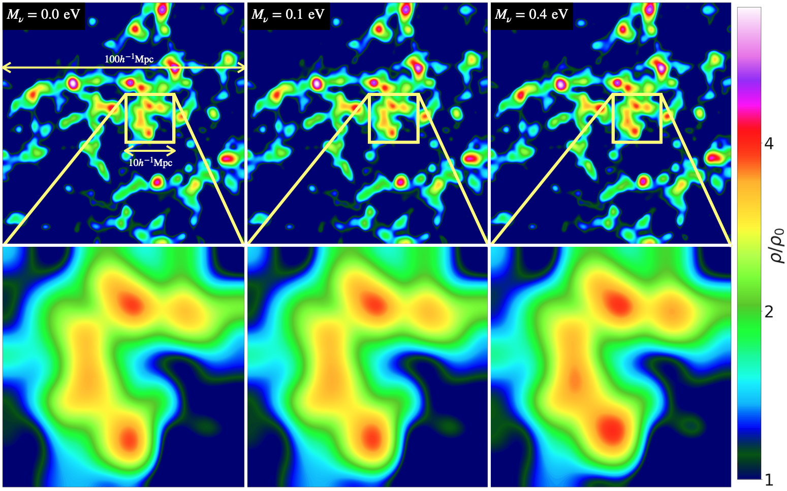
Figure 1.— Spatial projection of the DM overdensity field from three selected QUIJOTE simulations at $z=0$. Top panels display $100\times 100~{}[h^{-1}{\rm Mpc}]^{2}$ slices of the simulation cubes; bottom panels are enlargements of a small $10\times 10~{}[h^{-1}{\rm Mpc}]^{2}$ inset with identical spatial location. The fiducial massless neutrino cosmology (left), a massive neutrino model with $M_{\nu}=0.1~{}{\rm eV}$ (middle), and a massive neutrino scenario with $M_{\nu}=0.4~{}{\rm eV}$ (right) are shown, respectively. Although tiny, morphological and topological differences induced by a non-zero neutrino mass on the cosmic web network – as traced by the large-scale density field – are visually perceptible.

In this work, we use a subset of realizations from the QUIJOTE suite. The QUIJOTE simulations (Villaescusa-Navarro et al., 2020) are a set of 44,100 publicly available $N$-body runs spanning over 7000 cosmological models, following the gravitational evolution of $N_{\rm CDM}$ CDM plus $N_{\nu}$ neutrino particles (if present) with different resolutions (i.e., $256^{3}$, $512^{3}$, $1024^{3}$ particles per species). Initial conditions (ICs) are set at redshift $z_{\rm in}=127$ either adopting the Zel’dovich approximation (Zel’dovich, 1970) or via second order Lagrangian Perturbation Theory (2LPT). Moreover, the QUIJOTE suite contains standard, fixed, and paired fixed simulations, the difference being in the way ICs are generated. The input matter power spectra and transfer functions are obtained via the Boltzmann code CAMB (Lewis et al., 2000). All of the realizations are produced with the Three Particle Mesh (TreePM) code GADGET-III (Springel, 2005), over a periodic box size of 1$h^{-1}$Gpc, for a total volume of $44,100$ ($h^{-1}$Gpc)³. Snapshots are saved at $z=0,0.5,1,2,3$, respectively. The gravitational softening is set to $1/40$ of the mean inter-particle distance for all of the particle species, and the ICs random seeds are the same for an identical realization in different models, but vary from realization to realization within the same model. The baseline cosmological parameters are closer to those reported by the Planck Collaboration in 2018 (Planck Collaboration et al., 2020a), representing a flat (i.e., $\Omega_{\Lambda}+\Omega_{\rm m}=1$) massless neutrino $\Lambda$CDM model with the total matter density $\Omega_{\rm m}=0.3175$, the DE density parameter $\Omega_{\Lambda}=0.6825$, the baryon density $\Omega_{\rm b}=0.0490$, the primordial scalar spectrum power-law index $n_{\rm s}=0.9624$, the Hubble parameter $h=0.6711$, the DE equation of state (EoS) parameter $w=-1$, and the primordial power spectrum amplitude $A_{\rm s}=2.13\times 10^{-9}$ at the pivot scale $k_{\rm pivot}\equiv k_{0}=0.05~{}{\rm Mpc^{-1}}$. For convenience, these reference parameters are reported in the upper part of Table 1. Note that the normalization choice for $A_{\rm s}$ in the baseline massless neutrino cosmology implies $\sigma_{8}=0.834$ at $z=0$, with $\sigma_{8}$ the linear theory root mean square (rms) matter fluctuation in $8h^{-1}{\rm Mpc}$ spheres; by construction, all of the other realizations are tuned to match an identical $\sigma_{8}$ value at the present time.

In massive neutrino cosmologies, the rescaling method developed by Zennaro et al. (2017) is used to determine initial conditions. In addition, all of the massive neutrino realizations assume degenerate masses: the summed neutrino mass is indicated with $M_{\nu}$ in Table 1. Regarding neutrino implementations within the $N$-body framework, all of the the neutrino runs are performed employing a popular particle-based approach, treated as a collisionless and pressureless fluid (in the same fashion as CDM). Moreover, the forces at small scales for the neutrino species are also properly computed. The particle-based approach, despite shot noise challenges, is automatically able to capture the full nonlinear neutrino clustering and it accurately reproduces the nonlinear evolution at small scales – a crucial aspect for obtaining reliable and robust cosmological constraints. See Rossi (2017, 2020) for additional details on this implementation.

In our study, we use 100 independent realizations (i.e., having different initial random seeds) from the QUIJOTE suite for any of the following cosmologies: fiducial framework (massless neutrino scenario or ‘best guess’), massive neutrino model with $M_{\nu}=0.1~{}{\rm eV}$, and massive neutrino model with $M_{\nu}=0.4~{}{\rm eV}$, respectively. Specifically, we exploit the runs denoted as standard, characterized by Zel’dovich ICs at $z=127$. The resolutions considered are relatively low, $512^{3}$ particles per species, on a periodic box size of 1$h^{-1}$Gpc. We utilize full snapshots at $z=0,1,2,3$, in order to also assess redshift evolution effects. As previously noted, $\sigma_{8}(z=0)=0.834$ in all of the runs; hence, $A_{\rm s}$ varies with different neutrino masses. This normalization convention is what has been termed ‘NORM’ in Rossi (2020), and is well-motivated observationally, since $\sigma_{8}$ at the present epoch is effectively dictated by observational constraints. The main characteristics of the simulations adopted here are reported in the bottom part of Table 1, and more technical details can also be found in Villaescusa-Navarro et al. (2020).

As a visual example, Figure 1 shows a spatial projection of the dark matter (DM) overdensity field along the $x-y$ plane with a depth of $50h^{-1}{\rm Mpc}$ across the $z$-axis, obtained from three selected QUIJOTE simulations at $z=0$. From left to right, the plots refer to the fiducial massless neutrino cosmology run ($M_{\nu}=0.0~{}{\rm eV}$), the massive neutrino model with $M_{\nu}=0.1~{}{\rm eV}$, and the massive neutrino scenario with $M_{\nu}=0.4~{}{\rm eV}$, respectively. Top panels display $100\times 100~{}[h^{-1}{\rm Mpc}]^{2}$ slices of the simulation cubes, while bottom panels are enlargements of a small $10\times 10~{}[h^{-1}{\rm Mpc}]^{2}$ inset with identical spatial location and the same thickness as in the top figures. The normalized density fields are rendered using a rainbow palette, with the corresponding values indicated by the right side color bar. While rather small, morphological and topological differences induced by a non-zero neutrino mass are visually perceptible: they are quantifiable via the clustering statistics of critical points in the complex structure of the evolving cosmic web network, as we show in Section 4.

3. Methodology

In this section, we briefly describe our technique to construct density fields from the output of $N$-body simulations, extract and classify critical points, and subsequently perform clustering measurements in configuration space. We generically refer to this methodology as the ‘density threshold-based’ approach.

3.1. Density Threshold-Based Approach: Overview

For this first work, we adopt a technique centered on the extraction and classification of critical points from smoothed density fields. The construction of such fields is obtained via a grid interpolation strategy, directly from the DM particle distribution of $N$-body simulations. In essence, in the first step DM particles are turned into cells of given density, that are properly smoothed up to a desired scale. Critical points are then identified, and classified according to their type. Subsequently, those points are sorted in terms of density threshold (or rarity), and for a fixed rarity their clustering statistics is characterized as a function of $M_{\nu}$ and redshift. The advantage of this three-step procedure resides in its simplicity, ease of implementation, good efficiency, and effective numerical performance. In what follows, we briefly describe the three main building blocks of our pipeline.

3.2. Construction of Density Fields

We begin with the production of density fields, which are constructed from the DM particle output of selected QUIJOTE $N$-body realizations using the Python libraries for the analysis of numerical simulations (Pylians; Villaescusa-Navarro, 2018). Pylians are a set of Python, Cython, and C libraries that are helpful in the analysis of large-volume runs, providing a number of statistical tools – as well as routines to create and manipulate density fields. Specifically, at a fixed redshift, we build 3D density fields $\rho(\mathbf{x})$ from the spatial positions ($\mathbf{x}$) of $N$-body particles using a triangular-shape cloud (TSC) mass-assignment scheme to deposit particle masses into the grid; in this process, no weights are associated to each particle. Density contrast fields, defined as $\delta(\mathbf{x})=\rho(\mathbf{x})/\bar{\rho}-1$ with $\bar{\rho}$ the corresponding average background density, are readily inferred from the global knowledge of $\rho(\mathbf{x})$. We adopt $N_{\rm grid}=1024$ voxels per dimension on a regular grid spacing – corresponding to $2N_{\rm p}$, with $N_{\rm p}=512$ the number of particles per dimension in a given QUIJOTE simulation snapshot. We also tested different mass-assignment schemes, as well as a number of voxel choices for $N_{\rm grid}$, and found negligible dependence on our results.

3.3. Extraction and Classification of Critical Points

In the next step, fields are subsequently smoothed before the extraction and classification of critical points. More explicitly, DM density fields created from QUIJOTE snapshots are smoothed with a Gaussian kernel $W_{\rm G}$ over $R_{\rm G}=3h^{-1}{\rm Mpc}$ scales, using Py-Extrema. Smoothing is relevant for this density threshold-based methodology: we provide more extensive details related to our choice of the smoothing scale in Appendix A. We will also return on this important point in a companion publication, where we confront the present technique with a (fundamentally different) persistence-based approach – which instead does not rely directly on smoothing. In essence, the effect of smoothing is analogous to a resolution cut-off, erasing small-scale structures: at a given $z$-interval, structures of different sizes and masses are present, and therefore selecting an explicit $R_{\rm G}$ would correspond to averaging over specific density regions. A suitable smoothing choice is then relevant if we were to identify critical points with actual physical structures, as the effective typical size of such objects depends on the adopted smoothing scale of the density field: to this end, see the considerations presented in Section 4.1.

Once density fields have been properly smoothed, critical points are identified with the same detection algorithm adopted in Cadiou et al. (2020) and in Shim et al. (2021), based on a local quadratic estimator centered on a second order Taylor expansion of the density field about critical points – see also Gay et al. (2012) for additional details. Such expansion yields:

$$\mathbf{x}-\mathbf{x_{\rm c}}\sim(\nabla\nabla\rho)^{-1}\nabla\rho,$$ (1)

with $\mathbf{x_{\rm c}}$ the spatial position of the critical point. In essence, for each grid cell the gradient and Hessian of the density field are computed, Equation (1) is solved, and solutions found at a distance greater than 1 pixel are discarded via the requirement ${\rm max}_{\rm i}(|\mathbf{x}_{\rm i}-\mathbf{x}_{\rm c}|)<1~{}{\rm pixel}$ – with $i=1,2,3$: only the critical point closest to the center of the cell is retained. Subsequently, each cell enclosing a critical point is flagged, and an efficient loop is performed over flagged cells containing multiple critical points of the same type. In this process, critical points are classified according to their corresponding rank order. Specifically, the classification is based on the number of negative eigenvalues of the density Hessian – i.e., $0$ for voids (${\mathcal{V}}$ or minima); $1$ for walls (${\mathcal{W}}$ or ‘saddle 1’ or wall-type saddles); $2$ for filaments (${\mathcal{F}}$ or ‘saddle 2’ or filament-type saddles); $3$ for peaks (${\mathcal{P}}$ or maxima).

3.4. Clustering Measurements in Configuration Space

At this stage of the pipeline, critical points have been properly identified and classified. Next, all of the points are sorted according to the chosen density threshold $\nu=\delta/\sigma$, with $\delta$ the overdensity previously defined (but now referred to the smoothed density field), and $\sigma$ the corresponding rms fluctuation of the field. Following Shim et al. (2021), we adopt an identical ad hoc convention in defining rarity levels: namely, we always sample the population that provides the same abundance for a given type of critical point. This choice represents also a relevant point, that should be kept in mind later on, as it carries some impact on the interpretation of the results presented in Section 4 (i.e., the adopted rarity definition allows one to avoid density overlapping among critical points, thus enhancing more remarkable features in correlations).

Our rarity level definition can be formalized as follows. Let’s first introduce the notation $\alpha\in\{0,1,2,3\}\equiv\{{\mathcal{V}},{\mathcal{W}},{\mathcal{F}},{\mathcal{P}}\}$ to specify the critical point type. We will also use the indices $\ell$ and $k$ in place of $\alpha$, whenever necessary (i.e., $\alpha\equiv\ell,k$). In essence, for peak- and filament-type (respectively, void- and wall-type) critical points, we select ensambles with $\nu$ higher (respectively, lower) than a given threshold $\nu_{\alpha,\mathcal{R}}$, where $\mathcal{R}$ indicates the relative abundance cut. The threshold is then fixed as the rarity for each type of critical point $\alpha$ yielding the same relative abundances defined by the ratios:

$${n_{\rm C,\alpha}(\nu\geq\nu_{\alpha,\mathcal{R}})\over n_{\rm C,\alpha}}$$ (2)

with $\alpha\in\{\mathcal{P},\mathcal{F}\}\equiv\{3,2\}$ for peaks and filaments, respectively, and:

$${n_{\rm C,\alpha}(\nu\leq\nu_{\alpha,\mathcal{R}})\over n_{\rm C,\alpha}}$$ (3)

with $\alpha\in\{\mathcal{W},\mathcal{V}\}\equiv\{1,0\}$ for walls and voids, respectively. In the previous expressions, $n_{\rm C,\alpha}$ indicates the entire ensemble of critical points of type $\alpha$, while $n_{\rm C,\alpha}(\nu\geq\nu_{\alpha,\mathcal{R}})$ or $n_{\rm C,\alpha}(\nu\leq\nu_{\alpha,\mathcal{R}})$ represent the subset containing critical points of type $\alpha$ above or below the selected threshold $\nu_{\alpha,\mathcal{R}}$. For ease of notation, in what follows we define $\gamma\equiv\nu_{\alpha,\mathcal{R}}$, and also indicate $n_{\rm C,\alpha}(\nu\geq\gamma)$ or $n_{\rm C,\alpha}(\nu\leq\gamma)$ generically with $n_{\rm C,\alpha}^{\gamma}$. In our study we consider three cuts in rarity, namely $\mathcal{R}\in\{5,10,20\}$ – where the abundances are expressed in percentages.

We then compute the spatial clustering statistics of critical points above (below) threshold – i.e., real space two-point auto- and cross-correlations $\xi(r)$ as a function of the separation $r$ – using the Halotools platform (Hearin et al., 2017), equipped with efficient algorithms for calculating clustering statistics (including cross-correlations). For our two-point calculations in configuration space, we adopt the widely used minimal-variance Landy-Szalay (LS) estimator (Landy & Szalay, 1993) assuming periodic boundary conditions, and utilize random catalogs always at least 20 times bigger in size than the considered data. Specifically, for a given catalog $C^{\gamma}_{\alpha}$ of critical points above (below) a selected density threshold $\gamma$ having total size $n^{\gamma}_{\rm C,\alpha}$, and assuming a corresponding random catalog $R^{\gamma}_{\alpha}$ of total size $n^{\gamma}_{\rm R,\alpha}$ characterized by a random uniform probability distribution of points within the same volume, the LS estimator for the two-point correlation function $\xi_{\rm k\ell}^{\rm\gamma,\rm LS}$ above (below) $\gamma$ reads:

$$\xi_{\rm k\ell}^{\rm\gamma,\rm LS}=\sqrt{\eta\beta}{\langle C^{\gamma}_{\rm k}C^{\gamma}_{\rm\ell}\rangle\over\langle R^{\gamma}_{\rm k}R^{\gamma}_{\rm\ell}\rangle}-\sqrt{\eta}{\sqrt{\langle C^{\gamma}_{\rm k}R^{\gamma}_{\rm\ell}\rangle\langle C^{\gamma}_{\rm\ell}R^{\gamma}_{\rm k}\rangle}\over\langle R^{\gamma}_{\rm k}R^{\gamma}_{\rm\ell}\rangle}+1$$ (4)

where the normalization factors are specified by

$$\eta={(n^{\gamma}_{\rm R,\rm k}-1)(n^{\gamma}_{\rm R,\rm\ell}-1)\over n^{\gamma}_{\rm C,\rm k}n^{\gamma}_{\rm C,\rm\ell}}$$ (5)

and

$$\beta={n^{\gamma}_{\rm R,\rm k}n^{\gamma}_{\rm R,\rm\ell}\over(n^{\gamma}_{\rm C,\rm k}-1)(n^{\gamma}_{\rm C,\rm\ell}-1)}.$$ (6)

Note that all of the correlation measurements obtained via Equation (4) are reported as a function of the spatial separation $r$, conventionally expressed in units of $h^{-1}{\rm Mpc}$. Unless specified otherwise, we always use a bin size of $5h^{-1}{\rm Mpc}$: this choice is motivated by the study presented in Appendix A, where we also discuss smoothing and bin size effects on clustering measurements. Moreover, in order to accurately determine the spatial locations of the inflection points of the correlation functions at large scales (see Section 4.2), we also employ a ‘refinement’ technique where we adopt a smaller bin size of $1h^{-1}{\rm Mpc}$ in selected regions near such points.

4. Density Threshold-Based Approach: Results

This section contains the main results of our first analysis. After some basic considerations related to the ‘density threshold-based’ approach, we present here auto- and cross-correlation measurements of the clustering of critical points in massive neutrino cosmologies for a series of rarity levels, confronted with analogous computations in the baseline massless neutrino model. In particular, we show how massive neutrinos affect the BAO peak amplitudes of all of the critical point correlation functions above/below rarity threshold, as well as the positions of their corresponding inflection points at large scales. Finally, we also address redshift evolution effects.

In what follows, unless specified otherwise, we always express rarity thresholds $\mathcal{R}$ in percentage and consider two massive neutrino models having $M_{\nu}=0.1~{}{\rm eV}$ and $M_{\nu}=0.4~{}{\rm eV}$, respectively, besides the baseline massless neutrino scenario. Moreover, all of the measurements represent averages over 100 independent QUIJOTE realizations at fixed cosmology, and the associated errorbars are the corresponding $1\sigma$ variations.

4.1. Abundance and Visualization of Critical Points in Massive Neutrino Cosmologies

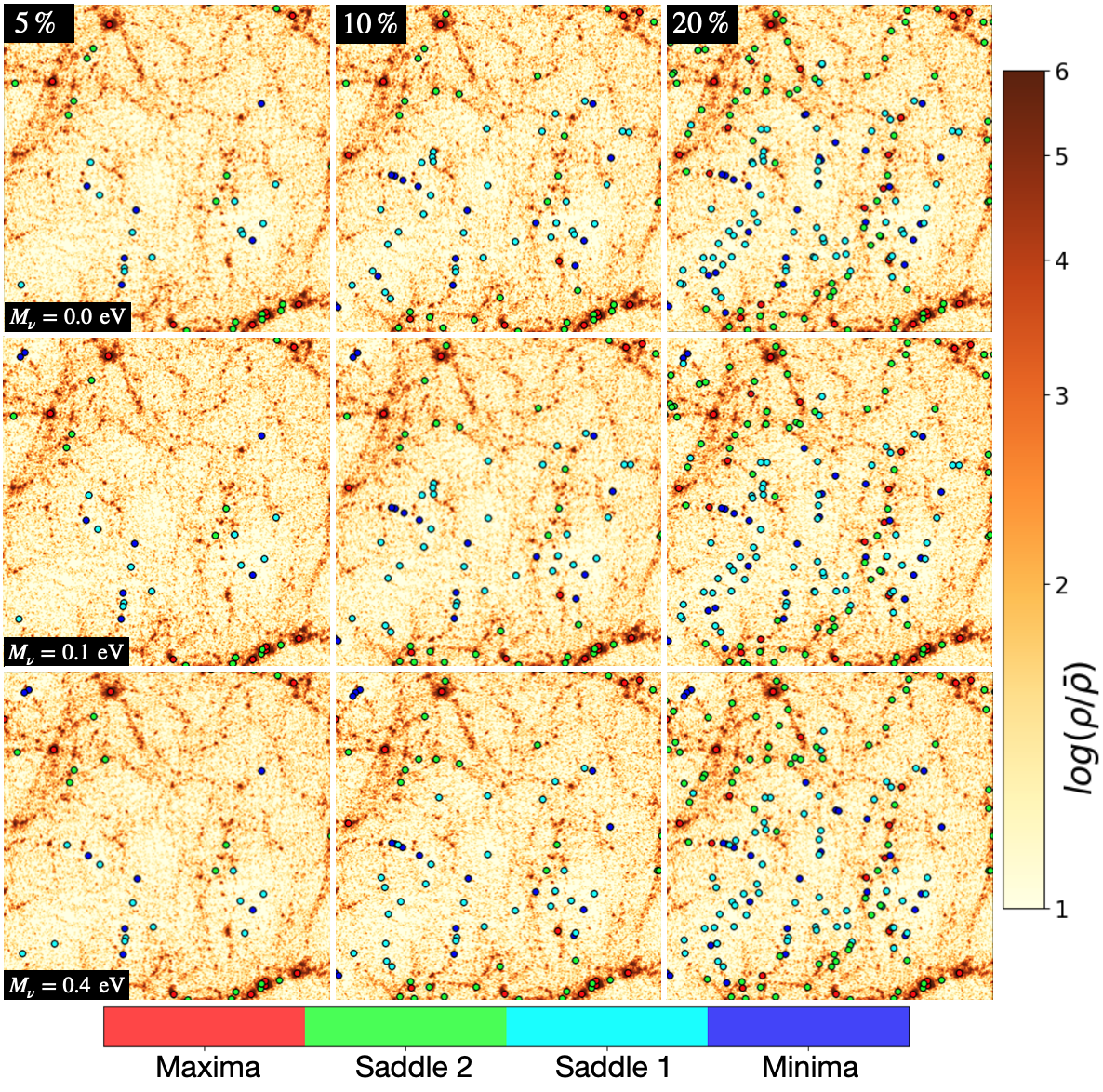
Figure 2.— Visualization of the spatial distribution of critical points (color-coded by their corresponding type) in massless and massive neutrino cosmologies at $z=0$, from small QUIJOTE-simulated cubic density patches of $100h^{-1}{\rm Mpc}$ side and $50h^{-1}{\rm Mpc}$ depth, as a function of rarity – with $\mathcal{R}$ increasing from left to right, as indicated in the various panels. Red, green, cyan, and blue are used respectively to display maxima, filament-saddles (‘saddle 2’), wall-saddles (‘saddle 1’), and minima. A ‘density threshold-based’ approach is adopted for the identification and classification of critical points, as reported in Section 3. See the main text for more details.

We begin with an instructive visualization of the geometrical distribution of critical points identified and classified via the ‘density threshold-based’ procedure described in Section 3. Figure 2 shows the spatial location of critical points in QUIJOTE-simulated patches at $z=0$, color-coded by type, for three different rarity thresholds. The squared patches in the figure are characterized by a side of $100h^{-1}{\rm Mpc}$ in the $x-y$ plane, and a $50h^{-1}{\rm Mpc}$ depth along the $z$-coordinate. The underlying normalized density fields are the results of sampling the density fields with Pylians assuming $N_{\rm grid}=1024$. Top panels refer to the baseline cosmology (massless neutrino scenario), middle panels are for a massive neutrino cosmology with $M_{\nu}=0.1~{}{\rm eV}$, while bottom panels display results for $M_{\nu}=0.4~{}{\rm eV}$. From left to right, the rarity threshold is increased in terms of relative abundance cut, corresponding to $5\%$, $10\%$, and $20\%$, respectively, via the selection criteria detailed in Section 3.4.

As anticipated before (i.e., Section 3.3), care must be taken in directly identifying critical points derived from a ‘density threshold-based’ approach with cosmological structures. This is primarily because such methodology relies on smoothing, and therefore the effective typical size of the LSS cosmic web constituents depends on the smoothing scale of the density field, which acts as a resolution cut-off. To this end, see also the discussion in Shim et al. (2021), who adopted a smoothing scale of $R_{\rm G}=6h^{-1}{\rm Mpc}$ corresponding to $\sim 10^{15}{\rm M_{\odot}}$ average density regions. As noted by the same authors, with such a choice of $R_{\rm G}$ only large voids can be resolved, and only 5% of all density peaks represent virialized galaxy clusters at $z=0$, while the rest is still in a collapse process. From Figure 2, one can deduce that decreasing the rarity threshold (namely, moving from the left to the right panels in the figure) provides a more detailed mapping of the corresponding underlying cosmological structures. This fact can be inferred from correlation function measurements: larger values of $\mathcal{R}$ manifest into smaller dispersions/scatter in $\xi(r)$, as we show in Sections 4.2 and 4.3. Moreover, it is also interesting to compare (even just at the visual level), the spatial distribution of critical points for a fixed rarity value with increasing neutrino mass: differences in the abundance and spatial location of critical points when $M_{\nu}\neq 0.0~{}{\rm eV}$ translate into morphological and topological differences that carry rich cosmological information.

In this regards, Table 2 reports the overall abundance of the entire set of critical points at $z=0$, classified by type, in the three cosmological frameworks considered in this work. These measurements are the results of running Py-Extrema on the smoothed density fields, and represent averages over 100 independent QUIJOTE realizations at fixed cosmology. Note that for a Gaussian field it is expected that the number of peaks ($\mathcal{P}$) and voids ($\mathcal{V}$) is similar, as well as the number of filaments ($\mathcal{F}$) versus walls ($\mathcal{W}$). Moreover, in Gaussian fields, the ratio between filaments and peaks ($\mathcal{F/P}$) or walls and voids ($\mathcal{W/V}$) is estimated to be $\sim 3.05$, and in addition the total number of extrema and saddle points is preserved at the first non-Gaussian perturbative order. Also, for sufficiently large volumes, the ratio between the number of peaks and walls over voids and filaments ($[\mathcal{P/W}]/[\mathcal{V/F}]$) in a Gaussian field is very close to unity throughout the entire $z$-evolution. This is because the genus topology, equal to the alternate sum of critical points, should be preserved, namely:

$$n_{\rm cp}^{\mathcal{P}}-n_{\rm cp}^{\mathcal{F}}+n_{\rm cp}^{\mathcal{W}}-n_{\rm cp}^{\mathcal{V}}=0~{},$$ (7)

with $n_{\rm cp}^{\rm(i)}$ the mean number density of peaks, filaments, walls, and voids – respectively.

However, nonlinear evolution breaks the symmetry between underdense and overdense regions. Table 3 summarizes all of the previous considerations, showing clear departures from Gaussianity – expected because of nonlinear structure formation, in addition to the presence of massive neutrinos. Note that the effect of a non-zero neutrino mass is represented by an overall decrement in the abundance of critical points, much more pronounced for higher neutrino masses. For peaks, this fact has repercussions at the level of the halo mass function, and it can be interpreted in the framework of the halo model – see e.g. Rossi (2017), their Section 4.3.

Table 2Total number of critical points at $z=0$, classified by type, for the three cosmologies considered in this work.

	${\mathbf{M_{\nu}{\rm[eV]}}}$	${\mathbf{z=0}}$
	0.0	$228,094\pm 382$
Minima ($\mathcal{V}$)	0.1	$227,770\pm 355$
	0.4	$226,527\pm 402$
	0.0	$680,088\pm 823$
Saddle 1 ($\mathcal{W}$)	0.1	$678,915\pm 775$
	0.4	$674,157\pm 797$
	0.0	$669,208\pm 858$
Saddle 2 ($\mathcal{F}$)	0.1	$667,952\pm 826$
	0.4	$662,960\pm 766$
	0.0	$223,951\pm 337$
Maxima ($\mathcal{P}$)	0.1	$223,571\pm 319$
	0.4	$222,031\pm 325$

Table 3Relevant abundance ratios of critical points at $z=0$ for the three cosmologies adopted in this study, highlighting the fact that nonlinear evolution as well as the effects of massive neutrinos (if present) break the symmetry between overdense and underdense regions – expected instead in a purely Gaussian field.

	${\mathbf{M_{\nu}{\rm[eV]}}}$	${\mathbf{z=0}}$
	0.0	$0.9818\pm 0.0022$
$\mathcal{P/V}$	0.1	$0.9816\pm 0.0021$
	0.4	$0.9802\pm 0.0023$
	0.0	$0.9840\pm 0.0017$
$\mathcal{F/W}$	0.1	$0.9839\pm 0.0017$
	0.4	$0.9834\pm 0.0016$
	0.0	$2.9888\pm 0.0059$
$\mathcal{F/P}$	0.1	$2.9877\pm 0.0056$
	0.4	$2.9859\pm 0.0056$
	0.0	$2.9816\pm 0.0062$
$\mathcal{W/V}$	0.1	$2.9807\pm 0.0058$
	0.4	$2.9761\pm 0.0063$
	0.0	$0.9661\pm 0.0028$
($\mathcal{P/W}$)/($\mathcal{V/F}$)	0.1	$0.9657\pm 0.0026$
	0.4	$0.9639\pm 0.0027$

4.2. Auto-Correlations of Critical Points in Massive Neutrino Cosmologies

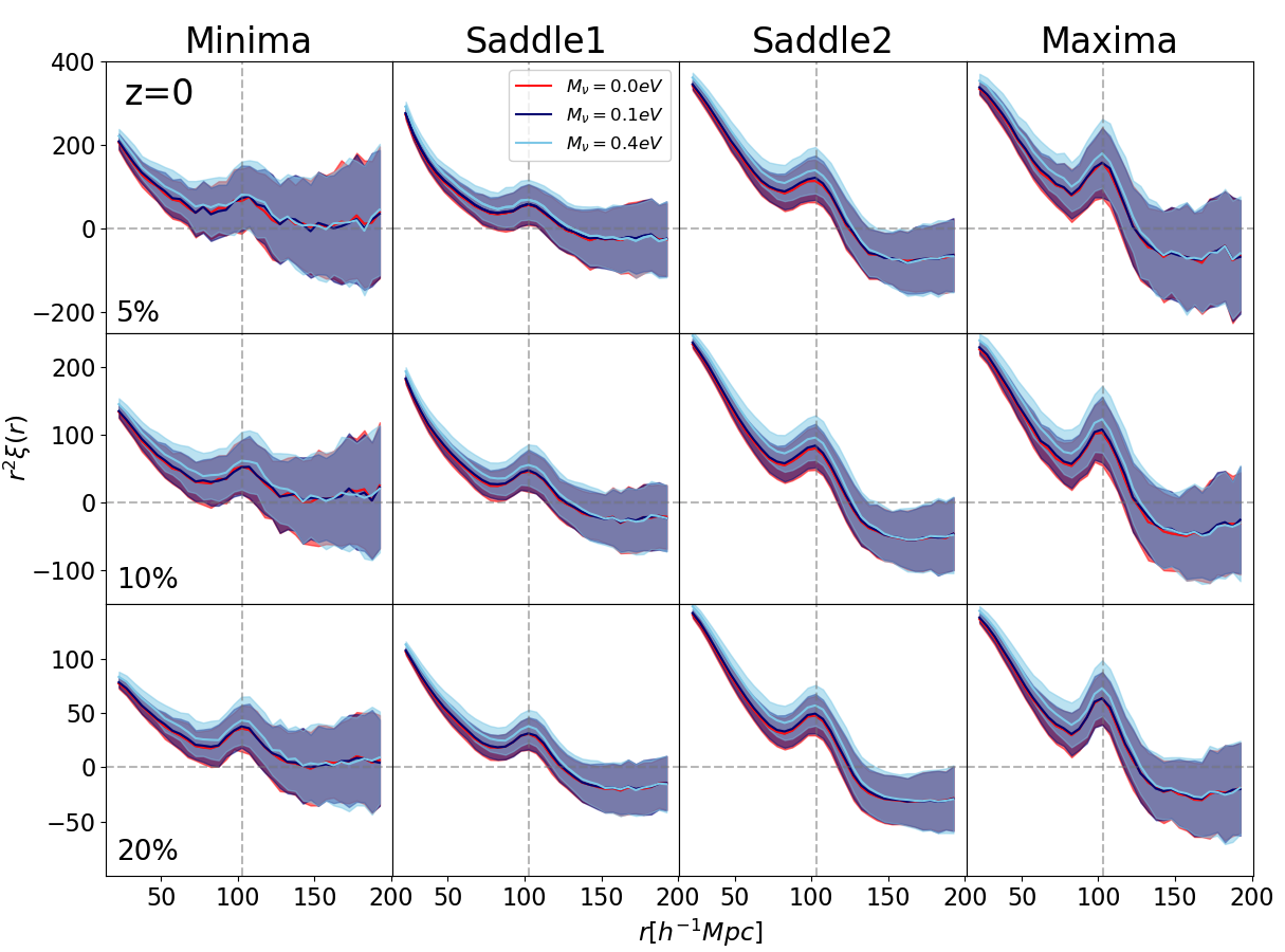
Figure 3.— Auto-correlations of critical points in configuration space at $z=0$, for three different rarity thresholds: $\mathcal{R}=5$ (top panels), $\mathcal{R}=10$ (middle panels), $\mathcal{R}=20$ (bottom panels). The two-point clustering statistics of minima, wall-type saddles, filament-type saddles, and maxima are shown from left to right, respectively. Three different cosmological models are considered, as indicated in the figure with contrasting colors: $M_{\nu}=0.0~{}{\rm eV}$ (red), $M_{\nu}=0.1~{}{\rm eV}$ (blue), and $M_{\nu}=0.4~{}{\rm eV}$ (cyan). Errorbars are estimated from averages of 100 independent QUIJOTE realizations for a given cosmology. BAO peaks are clearly visible in all of the panels, with the vertical dashed grey lines marking their exact scale ($102.5h^{-1}{\rm Mpc}$) – which is independent of critical point type, neutrino mass, and rarity.

Next, we move to auto-correlation measurements. Figure 3 shows the clustering statistics of critical points in configuration space at $z=0$ for three different rarity thresholds ($\mathcal{R}=5,10,20$), computed with the LS estimator via Equation (4). From left to right, minima, wall-type saddles, filament-type saddles, and maxima are displayed, respectively, for the three cosmologies considered in our analysis. BAO peaks are clearly visible in all of the panels, with the vertical dashed grey lines marking their exact scale (expressed with $r$ in $h^{-1}{\rm Mpc}$). Note that the positions of the BAO peaks are all the same, independently of critical point type, neutrino mass, and rarity – namely $102.5h^{-1}{\rm Mpc}$, which precisely coincides with the BAO expected location in the reference cosmology. This remarkable aspect is a clear indication that critical points trace the BAO peak similarly to DM, halos, and galaxies, and are faithful representations of their complementary structures.

Several interesting features can be inferred from Figure 3. First, it is evident that a non-zero neutrino mass generally corresponds to higher BAO amplitudes, regardless of the specific critical point type, and those amplitudes increase as $M_{\nu}$ is augmented. Namely, the larger the neutrino mass, the bigger the BAO amplitudes; this implies that it may be possible to infer neutrino mass signatures from such differential measurements, as we argue in this section. Moreover, the corresponding BAO amplitudes of minima and wall-type saddles are smaller than those of maxima and filament-type saddles. The similarity in shape between minima and saddles-1 (respectively, maxima and saddles-2) can be explained by considering how critical points below (above) threshold are selected – as detailed in Section 3.4. In fact, for minima and wall-type saddles the specific critical point abundance is determined from the lower-limit of the density field, while the opposite is done for maxima and filament-type saddles. Generally, extrema (i.e., minima and maxima) show noisier and less smoother correlation function shapes when compared to saddle-point clustering: notice in fact that their corresponding errorbars in Figure 3 are much larger. This is readily explained by the fact that the time evolution of extrema is more nonlinear than that of saddle points, as also reported by Cadiou et al. (2020) and Kraljic et al. (2022). In addition, more marked features in the BAO peaks and noisier correlation function shapes are seen with smaller rarity thresholds (see for example the top panels of the figure, where $\mathcal{R}=5$). This finding can be simply interpreted via linear bias, meaning that the more the tracer gets biased, the stronger the clustering – e.g., Kaiser (1984); Desjacques et al. (2018); Shim et al. (2021); Kraljic et al. (2022). Note that the effect of a rarity cut is similar to that of smoothing (see Appendix A, and also the previous references): an increase in smoothing implies a decrease in the number of volume elements along with an increase in bias, and consequently the spatial correlation function gets noisier because of enlarged statistical uncertainties, and its features appear more enhanced.

We then focus on two key features that can be inferred from our two-point correlation measurements in configuration space (i.e., Figure 3): namely, (1) the amplitudes of the various BAO peaks as a function of $\mathcal{R}$, and (2) the spatial locations of their corresponding inflection points at large spatial separations. The first aspect is quantified via Figures 4 and 5, while the second one is characterized by Figures 6 and 7.

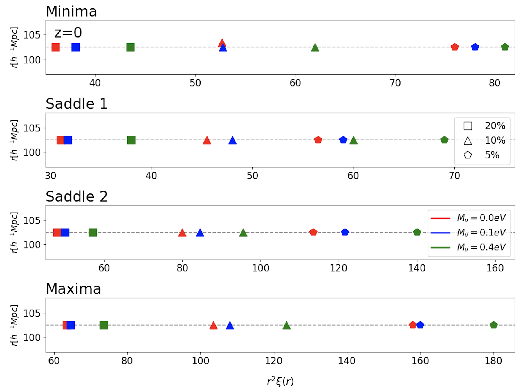
Figure 4.— BAO amplitudes ($r^{2}\xi$) versus their correspondent spatial position (i.e., $102.5h^{-1}{\rm Mpc}$, independent of critical point type, neutrino mass, and rarity) at $z=0$, derived from the auto-correlation measurements of minima, saddles-1, saddles-2, and maxima (top to bottom panels) reported in Figure 3. The three cosmological scenarios considered are represented with different colors (red: $M_{\nu}=0.0~{}{\rm eV}$; blue: $M_{\nu}=0.1~{}{\rm eV}$; green: $M_{\nu}=0.4~{}{\rm eV}$), and the rarity thresholds are indicated via contrasting symbols ($\mathcal{R}=5$, pentagons; $\mathcal{R}=10$, triangles; $\mathcal{R}=20$, squares).

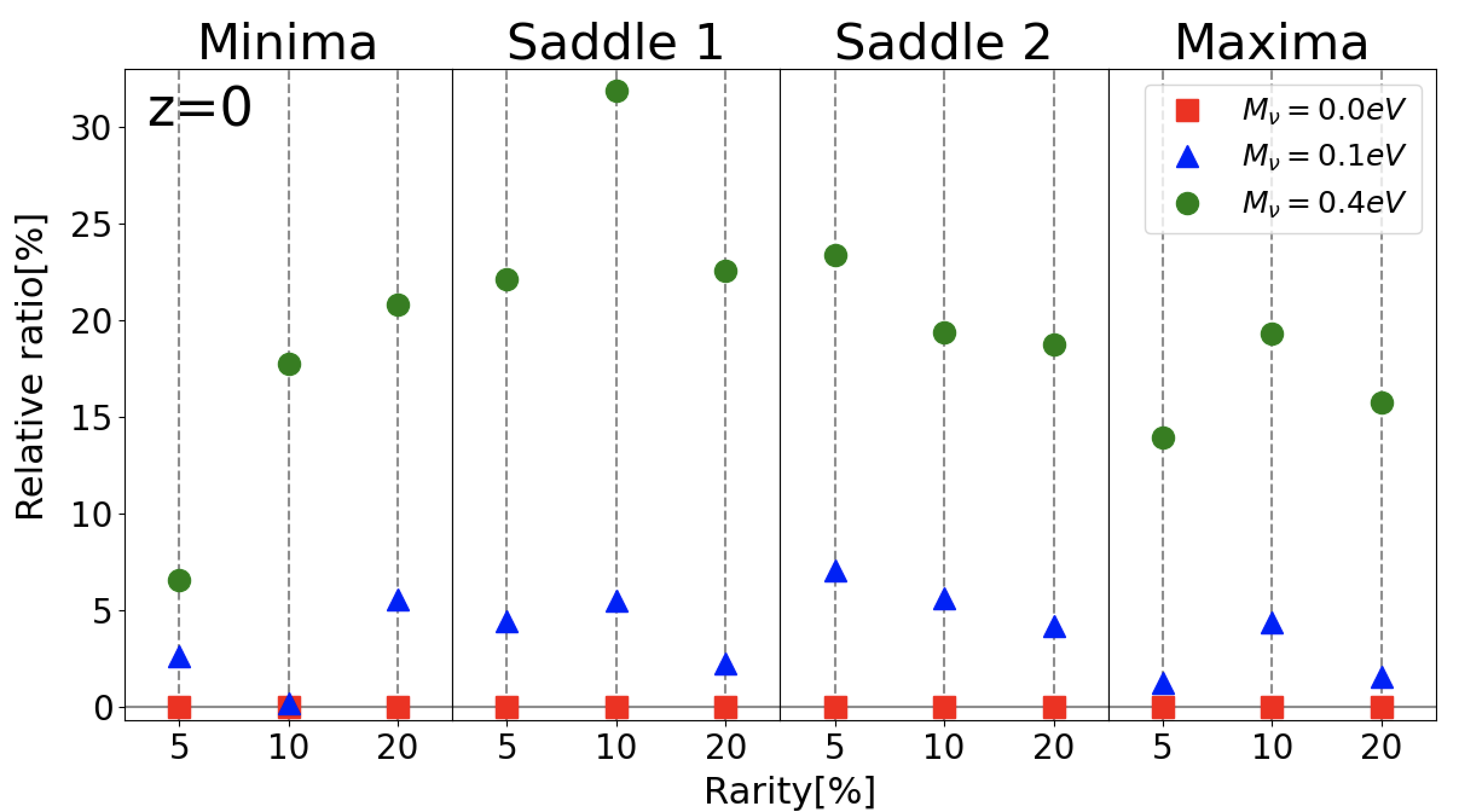
Figure 5.— BAO amplitudes in massive neutrino cosmologies, normalized by their correspondent values in a massless neutrino scenario and expressed in percentages as a function of rarity threshold at $z=0$. Colors refer to the same cosmological models examined in Figure 4. Departures from analogous measurements carried out in the baseline $M_{\nu}=0.0~{}{\rm eV}$ framework can reach up to $\sim 7\%$ at $z=0$, even for a relatively small neutrino mass of $M_{\nu}=0.1~{}{\rm eV}$.

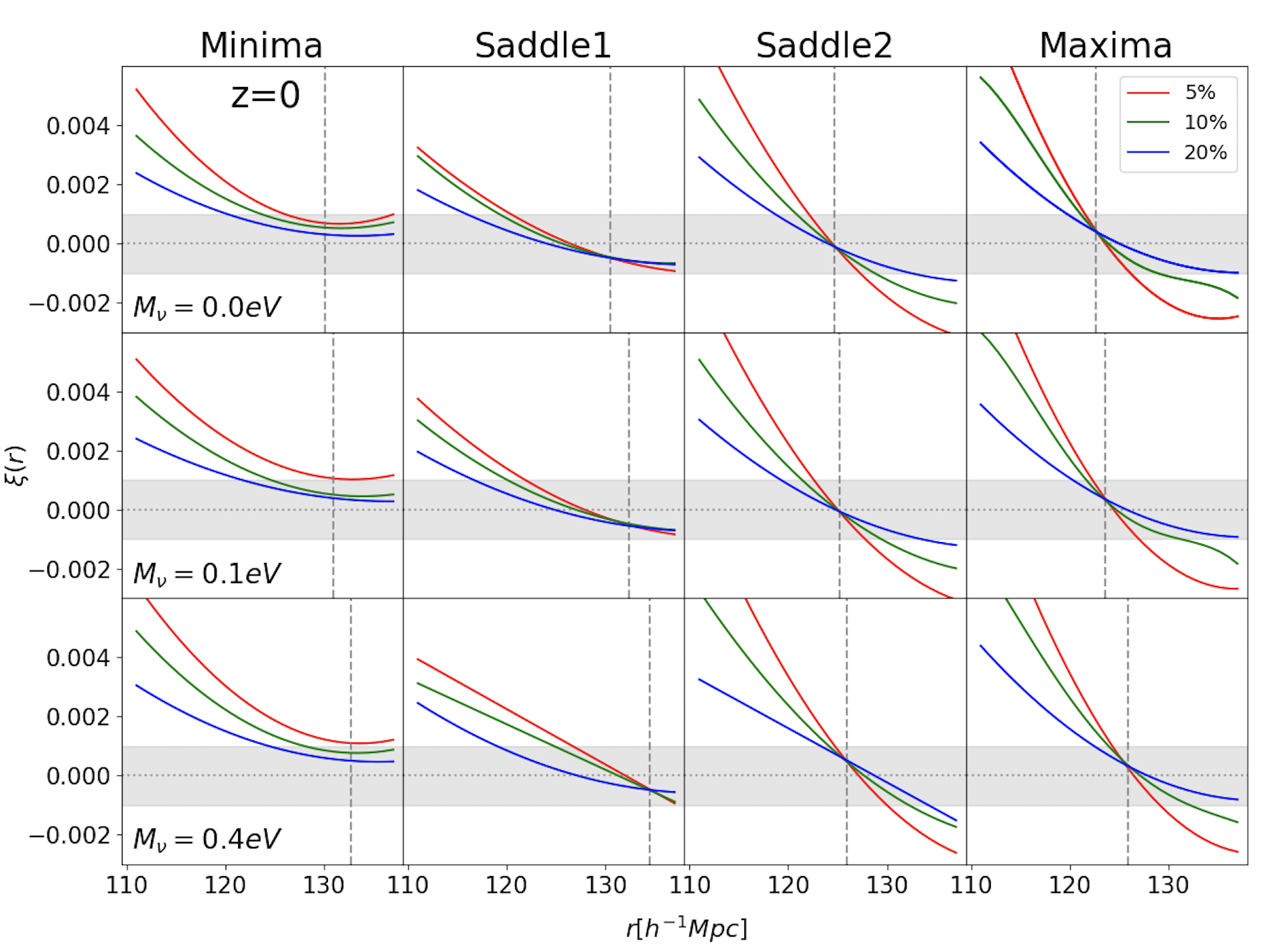
Figure 6.— Inflection scales of the critical point auto-correlation functions at large separation $r$ presented in Figure 3, indicating a clear sensitivity to massive neutrinos. In the various panels, measurements of $\xi(r)$ at $z=0$ are performed in the $110h^{-1}{\rm Mpc}<r<140h^{-1}{\rm Mpc}$ interval, using a refined binsize of $1h^{-1}{\rm Mpc}$. Top panels are for the baseline massless neutrino model, middle panels refer to the scenario with $M_{\nu}=0.1~{}{\rm eV}$, and bottom panels show the case of $M_{\nu}=0.4~{}{\rm eV}$. Results are averaged over 100 independent QUIJOTE realizations per given cosmology. The three rarity cuts are represented by different colors as indicated in the panels, and minima, wall-type saddles, filament-type saddles, and maxima are reported from left to right. Shaded horizontal errorbars indicate $\pm 0.1\%$ variations in $\xi$. Remarkably, the inflection scales (highlighted by the vertical grey dashed lines), independently of rarity, are altered by a non-zero neutrino mass.

Specifically, Figure 4 shows the measured BAO amplitudes ($r^{2}\xi$) at $z=0$ along the $x$-axis, versus their corresponding spatial position marked by horizontal grey dashed lines, for the three cosmological scenarios and the three rarity thresholds examined. From top to bottom, the four panels refer to minima, saddles-1, saddles-2, and maxima, respectively. Note in particular that the differences in terms of BAO amplitudes between a massless neutrino framework and a cosmology with $M_{\nu}=0.1~{}{\rm eV}$ are rather small, especially for the case of minima – for which their values almost coincide when $\mathcal{R}=10$; for this reason, in the top panel the red and blue triangles are slightly displayed along the $y$-direction, for the sake of clarity.

Such differences are better quantified in Figure 5, in terms of percentages. That is, we now display relative ratios among BAO amplitudes in massive neutrino cosmologies confronted with their correspondent values in a massless neutrino scenario, as a function of $\mathcal{R}$. Colors refer to the same cosmological models considered in Figure 4, but now the various symbols are also used to highlight those models, as reported in the figure. This visualization is quite useful, as it allows one to readily assess the effect of a non-zero neutrino mass on the BAO peaks inferred from the clustering of critical points in configuration space. In particular, as evident, departures from analogous measurements carried out in the baseline $M_{\nu}=0.0~{}{\rm eV}$ framework can reach up to $\sim 7\%$ at $z=0$ when $M_{\nu}=0.1~{}{\rm eV}$, and are much more pronounced for higher neutrino mass values.

From Figures 4 and 5 we can deduce a number of significant features. First, as in Shim et al. (2021), we find an amplification of the BAO peaks with rarity: namely, the amplitude of $\xi$ is higher (i.e., stronger clustering) for lower values of $\mathcal{R}$, regardless of the critical point type. And BAO features are further amplified by massive neutrinos, as quantified in the two plots. These effects are consistent with – and generalize – the findings of Peloso et al. (2015), who characterized the impact of neutrino masses on the shape and height of the BAO peak of the matter correlation function in real and redshift space, which contains relevant cosmological information; in the nonlinear regime the BAO peak increases with increasing $M_{\nu}$, and up to $1.2\%$ at $z=0$ when $M_{\nu}=0.30~{}{\rm eV}$, as reported by the same authors. Our approach based on critical points offers a more global multiscale perspective, since critical points carry remarkable topological properties and are good approximations for their corresponding LSS. Critical points are also less sensitive to systematic effects, and this is among the reasons why our auto-correlation BAO peak measurements show that departures from the corresponding massless neutrino scenario are more significant (up to $7\%$) even when $M_{\nu}=0.1~{}{\rm eV}$ – which is a value closer to the current stringent constraints on the summed neutrino mass reported in the literature. Furthermore, the spatial position of the BAO features in the various auto-correlations is robustly defined (i.e., $102.5h^{-1}{\rm Mpc}$) for all of the abundances considered, independently of critical point type and neutrino mass (hence an excellent standard ruler). Also, generally saddle-point statistics are more advantageous to use for extracting cosmological information because their cosmic evolution is less nonlinear (Gay et al., 2012; Shim et al., 2021); for example, the two-point auto-correlations of walls provide precious information on the characteristic sizes of voids. Finally, we note that all of the auto-correlation functions go to zero at large scales through an inflection point, an aspect that we address next.

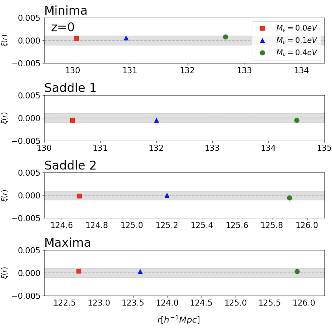
Figure 7.— Spatial positions of the inflection points of the auto-correlation functions at large scales for three different cosmologies, as inferred from Figure 6, ordered by critical point type (from top to bottom: minima, wall-type saddles, filament-type saddles, maxima). Red squares denote $M_{\nu}=0.0~{}{\rm eV}$, blue triangles are used for $M_{\nu}=0.1~{}{\rm eV}$, and green circles show $M_{\nu}=0.4~{}{\rm eV}$, at $z=0$. Grey horizontal errorbars indicate $\pm 0.1\%$ variations in $\xi$. A clear remarkable trend is seen as a function of neutrino mass.

To this end, Figure 6 shows another interesting and remarkable aspect of our analysis: not only the BAO amplitudes of all of the critical point auto-correlations are sensitive to massive neutrinos, but also their correspondent inflection scales – defined as the spatial positions at large $r$ where the correlation functions $\xi$’s of a given critical point type computed at different rarities $\mathcal{R}$ intersect (or are minimally distant), which also coincide with the spatial locations $r_{\rm inf}$ where $\xi(r_{\rm inf})\equiv 0$ (i.e., zero-crossings) within errorbars – are altered by a non-zero neutrino mass. Specifically, in Figure 6 we zoom into the $110h^{-1}{\rm Mpc}<r<140h^{-1}{\rm Mpc}$ interval and display the various $\xi(r)$’s measurements at $z=0$ and $\mathcal{R}=5,10,20$ for minima, wall-type saddles, filament-type saddles, and maxima – from left to right. All of the correlation function measurements are obtained with a ‘refined zoom-in’ technique: in essence, for a given cosmology and within the previously specified spatial interval, we recompute the two-point auto-correlations shown in Figure 3 for the three chosen rarity levels using a finer bin size ($1h^{-1}{\rm Mpc}$), and average the results over 100 independent QUIJOTE realizations. The inflection points are subsequently determined, and in the panels the vertical grey dashed lines indicate the spatial position of such points, while the shaded horizontal errorbars highlight variations of $\xi$ by $\pm 0.1\%$. For minima, the determination of this scale appears more challenging, but it still falls within the auto-correlation errorbars: this is likely due to the relatively small resolution of the simulations used in our study, that impacts underdense regions more severely than other cosmic web components, coupled with the fact that minima depart more significantly from linear theory.

The spatial positions of these inflection points at $z=0$ are reported in Figure 7, split by corresponding type. The shaded horizontal errorbars indicate the levels where $\xi$ varies by $\pm 0.1\%$; as evident, all of the inflection point spatial positions fall within this range.

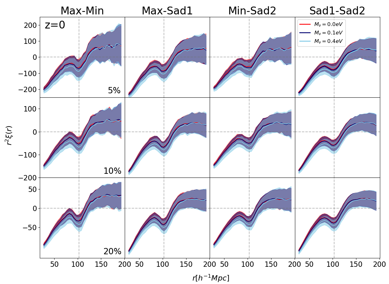
Figure 8.— Configuration-space cross-correlations of critical points having opposite overdensity sign, as a function of rarity threshold, at $z=0$. Colors and line styles same as in Figure 3. From left to right, $\mathcal{PV,PW,VF}$, and $\mathcal{WF}$ are displayed when $\mathcal{R}=5$ (top panels), $\mathcal{R}=10$ (middle panels), and $\mathcal{R}=20$ (bottom panels) – respectively. BAO features now appear as dips at $r=102.5h^{-1}{\rm Mpc}$, with the vertical dashed grey lines marking their exact scale.

The notable results presented in Figures 6 and 7 deserve some further attention. In particular, the interesting fact that such inflection points, independently of rarity, intersect also at the zero-crossing scale where $\xi(r_{\rm inf})\equiv 0$ within errorbars suggests that their positions can be well-described by standard linear theory, and we will return on this theoretical aspect in a forthcoming publication. Furthermore, these inflection points are also quite sensitive to massive neutrinos, with their spatial position increasing with augmented neutrino mass – within the interval [$120-135$]$h^{-1}{\rm Mpc}$. As in Shim et al. (2021), it is then intriguing to attempt an analogy, in a multiscale perspective, with the LP of the correlation function (Anselmi et al., 2016), which is likewise subject to massive neutrino effects (Parimbelli et al., 2021). Figure 7 shows indeed a clear sensitivity to a non-zero neutrino mass: through these inflection points it appears feasible to simultaneously quantify the perhaps unique signatures of $M_{\nu}$ on the four key web constituents (i.e., halos, filaments, walls, and voids).

4.3. Cross-Correlations of Critical Points in Massive Neutrino Cosmologies

We then move to cross-correlations, and carry out a similar analysis as performed for the auto-correlation case at $z=0$ in massless and massive neutrino cosmologies, for the same rarity thresholds previously considered. In general, cross-correlations are helpful in enhancing the signal-to-noise ratio (SNR) if used in combination with auto-correlations, and in mitigating the impact of systematics. In what follows, we compute all of the possible cross-combinations among extrema and saddle points: we show their clustering measurements in Figures 8 and 9.

Specifically, Figure 8 displays cross-correlations among overdense and underdense critical points having opposite overdensity sign – i.e., $\mathcal{PV,PW,VF,WF}$, from left to right, respectively. The computations are carried out in configuration space at $z=0$, as a function of rarity threshold and for the identical models considered in Figure 3, adopting the LS estimator (Equation 4). Clearly, cross-correlation shapes differ from those of auto-correlations (i.e., Figure 3). In essence, they are mirrored with respect to the $x$-axis: namely, the clustering is negative (anti-biased, or $\xi(r)<0$ in the $r$-interval of interest) until reaching zero at larger spatial separations. Hence, at scales relevant for our analysis, these cross-correlations are always negative, implying that overdense and underdense critical points are anti-correlated. Therefore, BAO features are now ‘reversed’ and appear as dips (rather than peaks) always at $r=102.5h^{-1}{\rm Mpc}$. Note that even in this case the spatial positions of the BAO dips are all identical, independently of critical point type pair, neutrino mass, and rarity. And, similarly to the auto-correlation measurements, BAO dips become more pronounced (i.e., showing a steeper negative amplitude) with increasing neutrino mass. As also pointed out by Shim et al. (2021) and Kraljic et al. (2022), anti-clustering arises because these critical point pairs are oppositely biased tracers of the underlying DM density field.

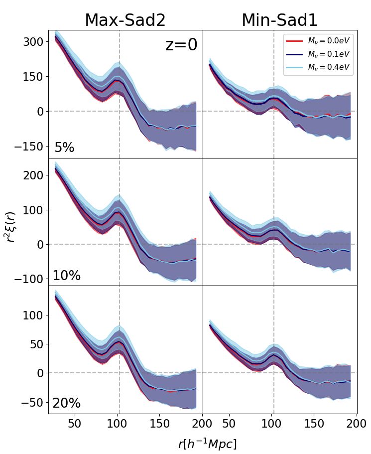
Figure 9.— Configuration-space cross-correlations of critical points characterized by an identical overdensity sign, as a function of rarity threshold, at $z=0$. Colors, line styles, rarity thresholds, and cosmologies same as those adopted in Figure 8. Left panels display cross-correlations of overdense critical point pairs ($\mathcal{PF}$), while right panels are for underdense critical point cross-correlations ($\mathcal{VW}$). Note that the shapes of the two-point cross-correlation clustering are akin to those of auto-correlation measurements (i.e., Figure 3), since here we consider cross-correlations of similarly biased tracers. BAO features appear as peaks at $r=102.5h^{-1}{\rm Mpc}$, with the vertical dashed grey lines marking their exact scale.

Figure 9 shows instead cross-correlations among overdense or underdense critical point pairs (namely, $\mathcal{PF}$ and $\mathcal{VW}$) – characterized by an identical overdensity sign (i.e., similarly biased tracers). Since now critical point pairs are described by the same overdensity sign, the overall shapes of their two-point clustering are comparable to those of auto-correlations (see again Figure 3). Hence, there is no anti-clustering at small separations, BAO peaks (local maxima) are detected at $r=102.5h^{-1}{\rm Mpc}$, and $\xi(r)$ approaches zero at large spatial separations. Also in this case, BAO peaks are further enhanced by massive neutrinos. Moreover, we note that $\mathcal{PF}$ cross-correlations show higher BAO amplitudes than $\mathcal{VW}$ cross-correlations at a fixed rarity threshold.

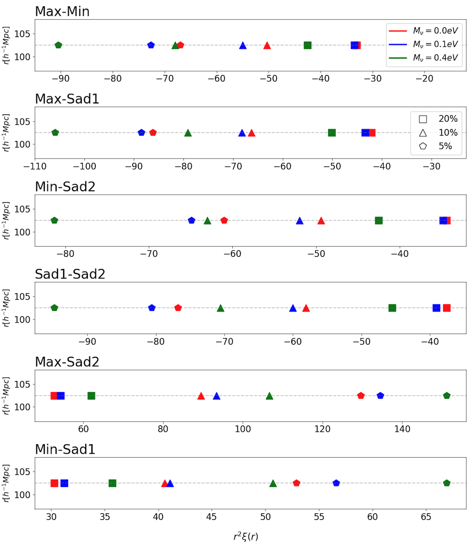
Figure 10.— BAO dip/peak amplitudes ($r^{2}\xi$) at $z=0$, versus their correspondent spatial positions ($r=102.5h^{-1}{\rm Mpc}$, independent of critical point type pair, neutrino mass, and rarity), inferred from the cross-correlation measurements presented in Figures 8 and 9. From top to bottom, $\mathcal{PV,PW,VF,WF,PF,VW}$ are shown, respectively. Different colors indicate distinct cosmologies, while contrasting symbols represent three choices of rarity thresholds. A clear trend as a function of neutrino mass can be readily inferred.

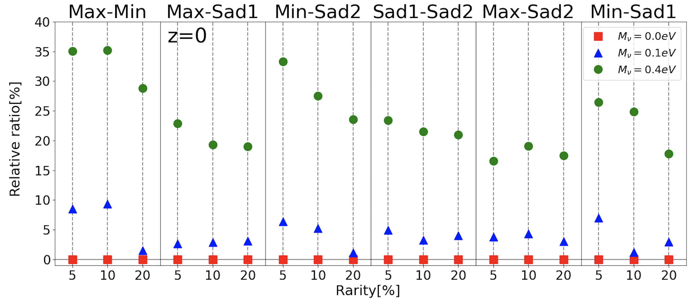
Figure 11.— BAO dip/peak amplitudes in massive neutrino cosmologies obtained from cross-correlation measurements, normalized by their correspondent values in a massless neutrino scenario and expressed in percentages as a function of rarity threshold at $z=0$ (with $\mathcal{R}=5,10,20$, respectively). Colors and symbols same as in Figure 5. In cross-correlations, departures from analogous measurements carried out in the baseline $M_{\nu}=0.0~{}{\rm eV}$ framework can be as high as $\sim 9\%$ at $z=0$ when $M_{\nu}=0.1~{}{\rm eV}$.

Figures 8 and 9 highlight another interesting aspect of our analysis, namely that the spatial positions of the BAO dips/peaks detected in cross-correlations are also robustly defined at the scale $r=102.5h^{-1}{\rm Mpc}$ (as for auto-correlations), independent of critical point type pair, neutrino mass, and rarity. Moreover, cross-correlations of similarly biased tracers exhibit a behavior comparable to those of auto-correlations, while BAO features are instead ‘reversed’ and manifest as dips for oppositely biased tracers. In both scenarios, a non-zero neutrino mass causes an overall enhancement of the amplitudes of the corresponding peaks/dips found in cross-correlations, much more pronounced for higher neutrino mass values. In addition, cross-correlations of minima with other critical point types show less noisy shapes (i.e., smaller errorbars), if compared with the auto-correlations of minima alone – which, on the contrary, present the noisiest correlation shapes. Also, $\mathcal{WF}$ cross-correlations display smooth and less noisy clustering than extrema cross-correlations. Finally, cross-correlations involving maxima and saddle points are also less noisier than maxima auto-correlations alone, emphasizing once more the benefits of cross-correlations.

Next, as previously done for auto-correlation measurements, we focus on two key aspects that can be inferred from the two-point cross-correlation estimations in configuration space (Figures 8 and 9): namely, (1) the amplitudes of the BAO dips/peaks as a function of $\mathcal{R}$, and (2) the spatial locations of their corresponding inflection points at large $r$-separations (as defined in the previous section). The first aspect is addressed in Figures 10 and 11, the second one is quantified via Figures 12 and 13.

In detail, Figure 10 shows the amplitudes ($r^{2}\xi$) of the BAO dips or peaks at $z=0$ for the various cross-correlations considered along the $x$-axis, versus their corresponding spatial position marked by horizontal grey dashed lines, for the three cosmologies examined and $\mathcal{R}=5,10,20$. A clear trend as a function of $M_{\nu}$ can be readily inferred: in essence, BAO dip/peak amplitudes are further enhanced (in absolute value terms) by the presence of massive neutrinos, and the enhancement is more significant with increased neutrino mass. Note also that $r^{2}\xi$ is negative in the first four panels since we are considering anti-biased critical points, while $r^{2}\xi$ is positive for similarly biased tracers.

Figure 11 better quantifies such differences in terms of percentages, in analogy to Figure 5 for auto-correlations: namely, we display relative ratios among cross-correlation BAO amplitudes in massive neutrino cosmologies, normalized by the correspondent values in a massless neutrino scenario, as a function of $\mathcal{R}$. As evident from the plot, departures from analogous cross-correlation measurements carried out in the baseline $M_{\nu}=0.0~{}{\rm eV}$ framework can reach even $\sim 9\%$ at $z=0$ when $M_{\nu}=0.1~{}{\rm eV}$, and are much more distinct for higher $M_{\nu}$ values. Interestingly, cross-correlations involving minima seem to be more effective in distinguishing small neutrino mass signatures (i.e., when $M_{\nu}=0.1~{}{\rm eV}$) than auto-correlations of minima alone.

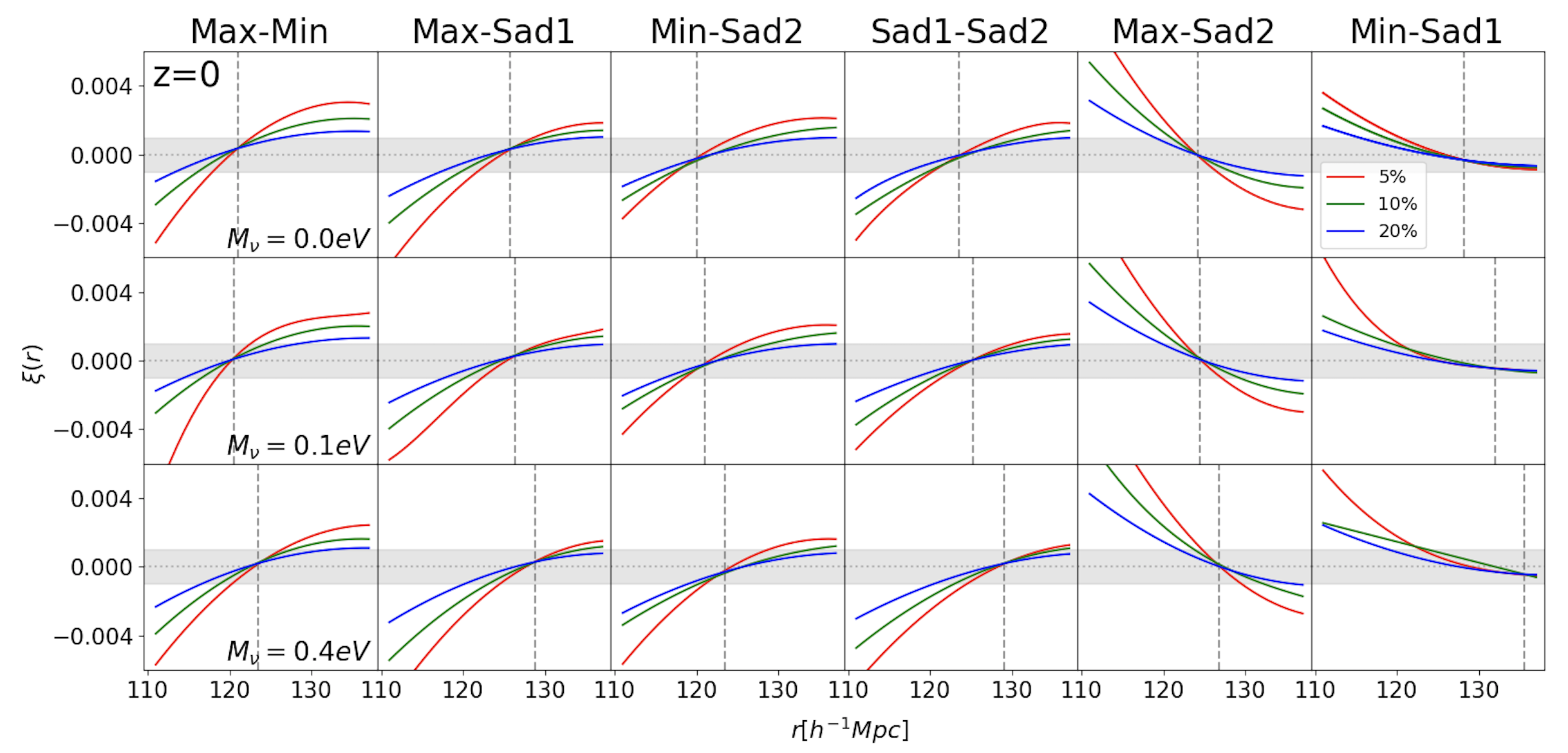
Figure 12.— Critical point pair cross-correlations: determination of the corresponding inflection scales in the interval $110h^{-1}{\rm Mpc}<r<140h^{-1}{\rm Mpc}$, from averages over 100 independent QUIJOTE realizations per cosmology at $z=0$, as specified in the panels. From left to right, $\mathcal{PV,PW,VF,WF,PF,VW}$ are shown, respectively, for three rarity thresholds ($\mathcal{R}=5,10,20$) represented by contrasting colors. Shaded horizontal errorbars display the levels where $\xi$ varies by $\pm 0.1\%$. In all of the panels, vertical grey dashed lines indicate the exact positions of the inflection scales, highlighting their sensitivity to neutrino mass effects.

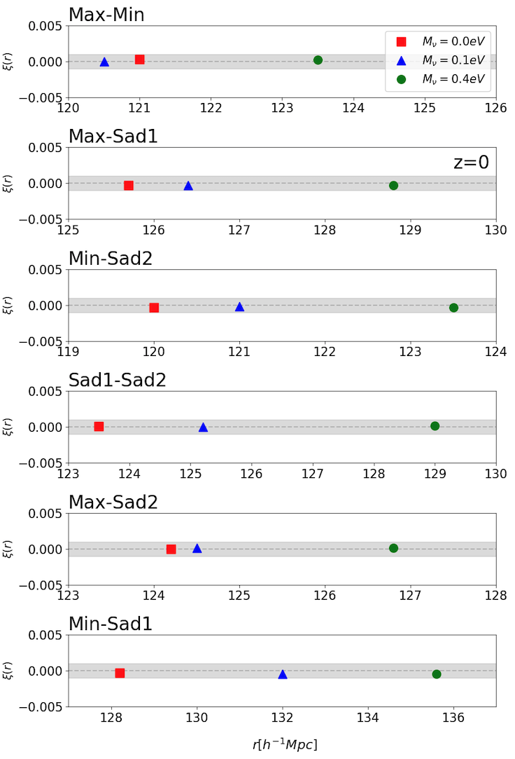
Figure 13.— Inflection scales of critical point pairs, inferred via $\mathcal{PV}$, $\mathcal{PW}$, $\mathcal{VF}$, $\mathcal{WF}$, $\mathcal{PF}$, and $\mathcal{VW}$ cross-correlation measurements at $z=0$ (from top to bottom, respectively). Red squares indicate $M_{\nu}=0.0~{}{\rm eV}$, blue triangles are for $M_{\nu}=0.1~{}{\rm eV}$, and green circles denote $M_{\nu}=0.4~{}{\rm eV}$. Shaded horizontal errorbars highlight $\pm 0.1\%$ variations in $\xi$: all of the inflection point spatial positions fall within this range.

Finally, we examine the cross-correlation inflection points at large scales. In this respect, Figure 12 illustrates the remarkable fact that all of the inflection scales of the critical point pair cross-correlations are also sensitive to neutrino mass effects, independently of rarity (note the analogy with Figure 6). Specifically, we consider the $110h^{-1}{\rm Mpc}<r<140h^{-1}{\rm Mpc}$ interval, recompute all of the two-point cross-correlations shown in Figures 8 and 9 with a refinement procedure, and average the results over 100 independent QUIJOTE realizations at $z=0$. Inflection points are subsequently determined, as indicated in the panels by the vertical grey dashed lines, where from left to right we display $\mathcal{PV,PW,VF,WF,PF,VW}$, respectively – while the shaded horizontal errorbars highlight the levels where $\xi$ varies by $\pm 0.1\%$.

The spatial positions of the inflection points determined from all of the possible cross-correlations at $z=0$ are also reported in Figure 13, split by corresponding pair type. With the exception of the $\mathcal{PV}$ case when $M_{\nu}=0.1~{}{\rm eV}$ (top panel), we detect a clear trend related to the inflection point positions in neutrino cosmologies: namely, the spatial locations of all of the inflection points are amplified by massive neutrinos, as a function of their mass. The apparent disagreement with this trend represented by the $\mathcal{PV}$ cross-correlation measurement when $M_{\nu}=0.1~{}{\rm eV}$ (top panel) is likely related to the challenges in determining the inflection scale using minima (see for comparison the left panels of Figure 6), considering also their selection procedure (i.e., points below rarity threshold, see the details in Section 3.4). Remarkably, even in cross-correlations we find an enhanced sensitivity of the inflection scales to massive neutrino effects.

4.4. Clustering of Critical Points in Massive Neutrino Cosmologies: Redshift Evolution Effects

Finally, we briefly address redshift evolution effects, in relation to the clustering properties of critical points. To this end, Figures 14 and 15 provide some examples for auto-correlations: the position of the BAO peaks ($r=102.5h^{-1}{\rm Mpc}$, independent of redshift) is marked by vertical dashed grey lines.

Specifically, Figure 14 displays the clustering statistics of critical points in configuration space at $z=1$ (top panels), $z=2$ (middle panels), and $z=3$ (bottom panels), for a rarity choice corresponding to $\mathcal{R}=20$ and varying cosmologies. We adopt the same stylistic conventions as in Figure 3. In the various panels, we maintain the same $x-y$ scale for a better visual characterization of the redshift impact in the clustering properties. At any given redshift and for all of the critical point types, a non-zero neutrino mass causes an enhancement of the BAO peak amplitudes: the enhancement is more significant for higher neutrino mass values (see for example the $M_{\nu}=0.4~{}{\rm eV}$ case).

To appreciate possible redshift evolution effects more clearly, in Figure 15 we now show auto-correlation functions for the same rarity threshold previously examined and within a fixed cosmological model – while we vary the redshift in each panel by considering $z=1$ (purple), $z=2$ (dark green), and $z=3$ (light green), respectively, as specified by different colors in the figure inset. Similarly as in Figure 14, from left to right we indicate minima, wall-type saddles, filament-type saddles, and maxima.

Around the scale of BAO peaks, all of the auto-correlations show small evolution with redshift. And, as expected, $z$-evolution (although weak) is more relevant for the auto-correlations involving the most non-linear critical points (peaks, voids), while those involving less non-linear critical points (filaments, walls) appear mostly insensitive to redshift evolution effects. In particular, the evolution seems more prominent for minima. Moreover, we find a similar trend in cross-correlation measurements.

Therefore, as also noted in Shim et al. (2021), the overall insensitivity to redshift especially for saddle statistics makes the clustering of critical points a topologically robust alternative to more standard clustering methods.

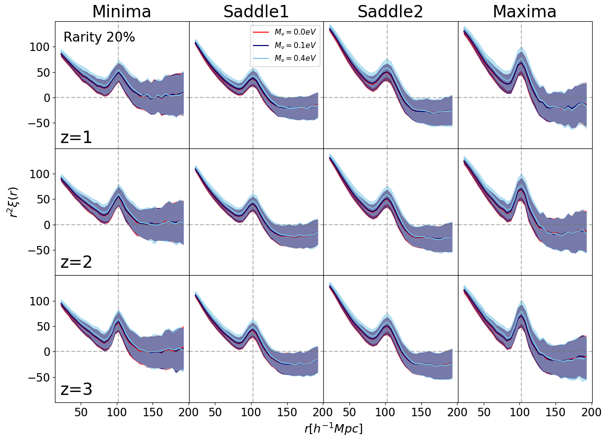
Figure 14.— Clustering statistics of critical points: redshift evolution at fixed rarity threshold ($\mathcal{R}=20$) and varying cosmologies (red lines: baseline massless neutrino model; blue lines: $M_{\nu}=0.1~{}{\rm eV}$; cyan lines: $M_{\nu}=0.4~{}{\rm eV}$). Top panels are for $z=1$, middle panels refer to $z=2$, and bottom panels are for $z=3$. Minima, wall-type saddles, filament-type saddles, and maxima are represented – from left to right.

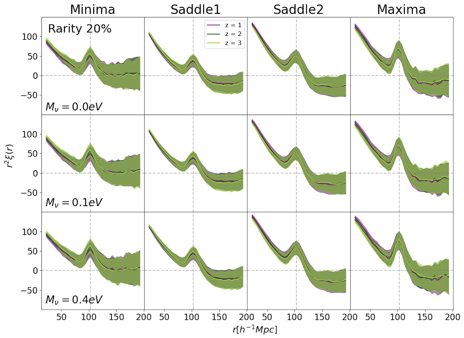
Figure 15.— Clustering statistics of critical points: redshift evolution at fixed rarity threshold ($\mathcal{R}=20$) and within a given cosmological framework. Top panels are for the baseline massless neutrino model, in the middle panels $M_{\nu}=0.1~{}{\rm eV}$, and bottom panels display $M_{\nu}=0.4~{}{\rm eV}$. In each panel, contrasting colors represent different redshifts ($z=1,2,3$) – as specified by the inset. While at intermediate $r$-separations all of the auto-correlations show little evolution with redshift, in general, even if small, $z$-evolution is more relevant for the correlations involving the most non-linear critical points (i.e., extrema).

5. Summary and Outlook

Determining the neutrino mass scale and type of hierarchy are primary targets for all of the ongoing and upcoming large-volume astronomical surveys, as well as a major goal of future space missions. Current limits from cosmology are already putting considerable pressure on the IH scenario as a plausible possibility for the neutrino mass ordering (Planck Collaboration et al., 2020a; eBOSS Collaboration et al., 2021), and a direct neutrino mass detection, or at least more competitive upper bounds on $M_{\nu}$, are expected in the next few years from Stage-IV cosmological experiments. Moreover, gaining a deeper theoretical understanding of the impact of massive neutrinos on structure formation particularly at small scales and on the major observables typically used to characterize neutrino mass effects are necessary, to obtain robust constraints free from systematic biases.

Traditional methodologies for detecting and constraining neutrino mass effects from cosmology generally rely on a single observable, or on a limited scale-range. Examples include CMB gravitational lensing, the ISW effect in polarization maps, as well as a large number of LSS tracers such as 3D galaxy clustering via the matter power spectrum, bispectrum, cosmic shear, galaxy clusters, voids statistics, and much more.

In this work, we pursued a novel and different multiscale route, exploiting the remarkable topological properties of critical points – whose positions and heights at fixed smoothing scale retain precious cosmological information (Sousbie et al., 2008; Pogosyan et al., 2009; Gay et al., 2012; Cadiou et al., 2020; Shim et al., 2021; Kraljic et al., 2022). Besides being more robust to systematic effects, and in particular to non-linear evolution, clustering bias, and redshift space distortions, such special points are useful because they represent a meaningful and efficient compression of information of the 3D density field capturing its most significant features; thus, they provide a more fundamental and global view of the cosmic web as a whole. The overall weak sensitivity to systematics ultimately stems from their close relationship with the underlying topology, as described for example by the genus or Betti numbers. And, noticeably, all of the topological changes of a space occur only at critical points, and critical points of the density field are responsible for both the formation and destruction of a given feature.

For the first time, we characterized their clustering statistics in massive neutrino cosmologies, addressing the critical point sensitivity to small neutrino masses with the goal of identifying (possibly unique) neutrino multiscale signatures on the corresponding web constituents – i.e., halos, filaments, walls, and voids. We carried out our measurements on a subset of realizations from the QUIJOTE suite (Villaescusa-Navarro et al., 2020), using full snapshots at $z=0,1,2,3$ for a choice of representative neutrino masses, as explained in Section 2. Exploiting a ‘density threshold-based’ methodology, described in Section 3, we computed critical point auto- and cross-correlation functions in configuration space for a series of rarity thresholds, and also characterized redshift evolution effects. Our major results, presented in Section 4 and summarized through Figures 3-15, are focused on BAO scales and are centered on two key aspects: (1) the multiscale effects of massive neutrinos on the BAO peak amplitudes of all of the critical point correlation functions above/below rarity threshold, and (2) the multiscale effects of massive neutrinos on the spatial positions of their correspondent correlation function inflection points at large scales.

The main findings and pivotal outcomes of this first work can be summarized as follows:

• The BAO scale determined from critical point auto- and cross-correlation measurements above/below rarity threshold is always robustly detected at $102.5h^{-1}{\rm Mpc}$. The scale coincides with the BAO expected location in the reference cosmology, and it is independent of critical point type, neutrino mass, and rarity. This remarkable aspect is a clear indication that critical points trace the BAO peak similarly to DM, halos, and galaxies, and are faithful representations of their corresponding structures.

• All of the BAO peaks in auto-correlations are amplified with decreasing rarity: the amplitude of $\xi$ is higher for lower values of $\mathcal{R}$, regardless of the critical point type. Similarly, such amplifications of the BAO peaks are also found in critical point cross-correlations characterized by an identical overdensity sign (i.e., $\mathcal{PF}$ and $\mathcal{VW}$, similarly biased tracers), and in the BAO dips of the critical point cross-correlations of overdense and underdense regions having opposite overdensity sign (i.e., $\mathcal{PV,PW,VF,WF}$). Cross-correlations of similarly biased tracers exhibit a behavior comparable to those of auto-correlations, while BAO features are ‘reversed’ and manifest as dips for oppositely biased tracers. Note also that the effect of a rarity threshold is also similar to that of smoothing.

• Massive neutrinos affect the BAO peak amplitudes of all of the critical point auto- and cross-correlation functions above/below rarity threshold. Differences at $z=0$ between a massless neutrino cosmology and a scenario with $M_{\nu}=0.1~{}{\rm eV}$ can reach up to $\sim 7\%$ in auto-correlations, and $\sim 9\%$ in cross-correlations. BAO peaks/dips become more pronounced (in absolute value terms) with increasing neutrino mass.

• Inflection scales are detected around $125h^{-1}{\rm Mpc}$, both from auto- and cross-correlation measurements. Their exact values differ according to the critical point type. And, remarkably, inflection scales are altered by a non-zero neutrino mass – independently of rarity – with their spatial position increasing with augmented neutrino mass.

• Generally, extrema show noisier and less smoother auto- and cross-correlation function shapes when compared to saddle-point statistics, as the time evolution of extrema is more nonlinear than that of saddles. Hence, saddle point statistics may be more advantageous for extracting cosmological information, and in relation to neutrino mass constraints.

• Around the BAO scale, all of the auto-correlations barely show evolution with redshift. Also, as expected, $z$-evolution (although weak) is more relevant for auto-correlations involving the most nonlinear critical points (peaks, voids), while those involving less nonlinear critical points (filaments, walls) seem mostly insensitive to redshift evolution effects. And, at any given redshift that we considered and for all of the critical point types, a non-zero neutrino mass causes an enhancement of the BAO peak amplitudes, which appears more significant for higher neutrino mass values.

Our novel approach to neutrino mass effects, based on the statistics of critical points, offers a multiscale perspective, since such points carry remarkable topological properties and are faithful representation of their corresponding LSS. Moreover, critical points are also less sensitive to systematics, and this is among the reasons why our auto- and cross-correlation measurements appear more sensitive to neutrino signatures than analogous measurements performed on the total matter correlation function. In this view, part of our results can be seen as a multiscale generalization of the Peloso et al. (2015) findings about the impact of massive neutrinos on BAOs, and perhaps also as the multiscale extension of the LP of the spatial correlation function – which is also subject to non-zero neutrino mass effects (Parimbelli et al., 2021). In addition, our technique is complementary to more traditional methods, and can be combined with such methods to enhance the SNR: we will address this aspect in upcoming publications. Hence, our study is particularly relevant for ongoing and future large-volume redshift surveys such as DESI and the Rubin Observatory LSST, that will provide unique datasets suitable for establishing competitive neutrino mass constraints, as well as for future high-redshift probes like the WHT Extended Aperture Velocity Explorer (WEAVE; Dalton et al., 2012).

To this end, much work still remains to be performed in order to bring the methodologies presented here to real data applications: the current study is just the first of a series of investigations that aim at exploring the sensitivity of critical points and critical events to massive neutrinos, and more generally in relation to the dark sector. Ongoing efforts are along two major directions: towards galaxy clustering at relatively low redshift, and towards the high-$z$ universe as mapped for example by the Ly$\alpha$ forest. In forthcoming publications, we will focus on these aspects, and also characterize the relation of our methodology with a persistence-based approach. Moreover, we will show how the combined multiscale effects presented here – inferred from the clustering of critical points – can be used to set upper limits on the summed neutrino mass and infer the type of hierarchy.

Appendix A A. Analysis Technicalities: On Bin Size and Smoothing

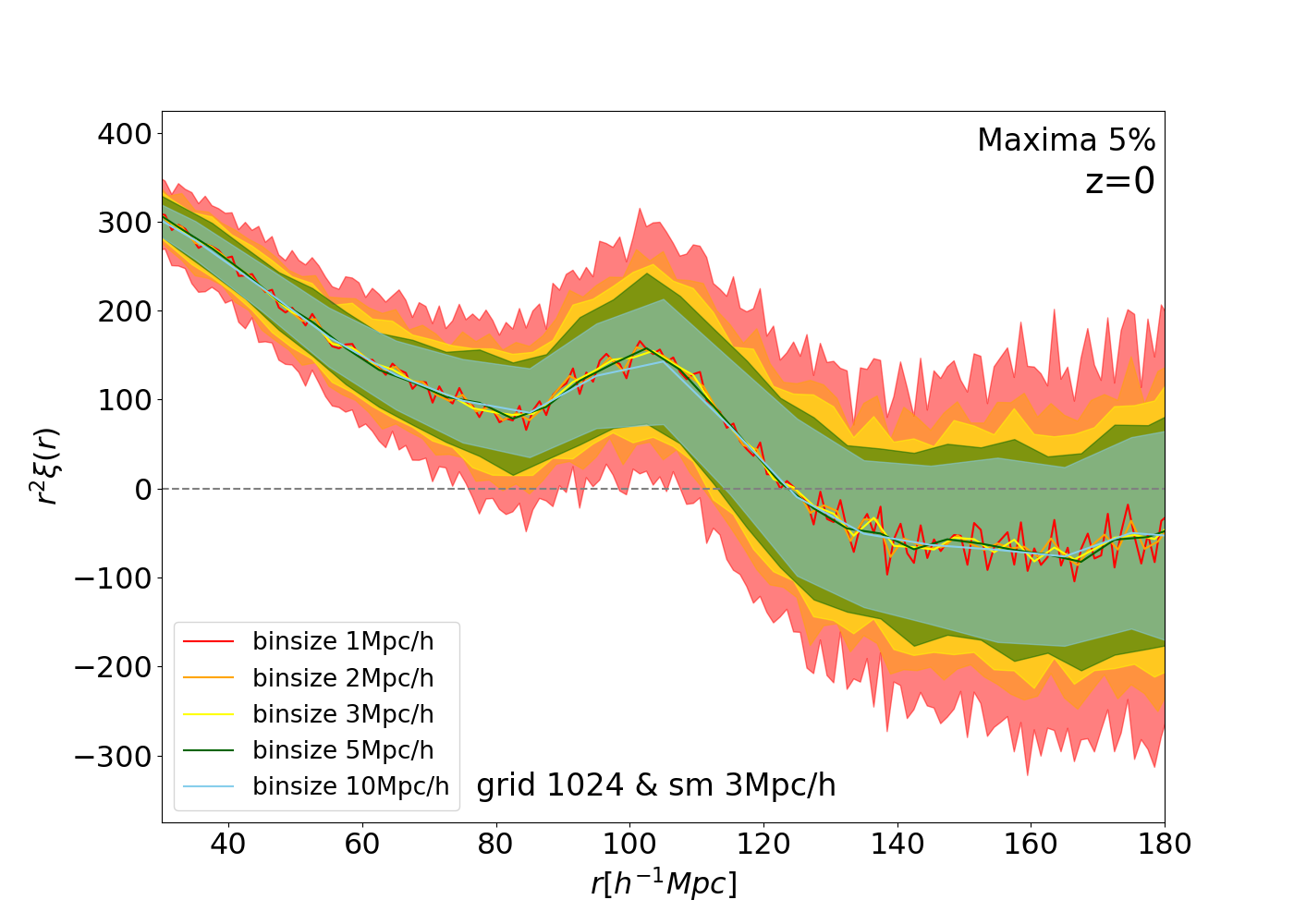
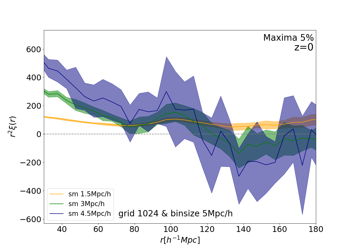
Figure 16.— Critical point auto-correlation tests related to the bin size choice [left], and to the selection of the smoothing scale [right]. In both panels, we consider only maxima at $z=0$ for a rarity $\mathcal{R}=5$ and the number of voxels $N_{\rm grid}=1024$. In particular, altering the bin size does not affect the overall shape of the auto-correlation function (including the location of the BAO peak and the zero-crossing scale), while smoothing acts similarly to the effect of a rarity choice.

In this section, we provide more details on the bin size used in the computations of the auto- and cross-correlation functions presented in the main text, and on the smoothing scale adopted. Specifically, the left panel of Figure 16 shows the effect of a varying bin size on the critical point auto-correlation function. As an example, we consider only maxima at $z=0$ for a rarity threshold $\mathcal{R}=5$, when $N_{\rm grid}=1024$ and the smoothing scale is fixed to $R_{\rm G}=3h^{-1}{\rm Mpc}$. Contrasting colors are used to indicate different bin sizes ($r_{\rm bin}$), with $r_{\rm bin}=1,2,3,5,10$, respectively, in units of $h^{-1}{\rm Mpc}$. As evident from the plot, altering the bin size does not affect the overall shape of the auto-correlation function, including the location of the BAO peak and the zero-crossing scale. However, clearly smaller bin sizes manifest noisier $\xi$ shapes (i.e., bigger errorbars). Our choice of $5h^{-1}{\rm Mpc}$, represented by the green line with errorbars in the panel, guarantees a sufficiently smooth $\xi$: this is what is typically assumed in surveys like eBOSS for characterizing two-point correlation functions. Note also that we adopt a smaller bin size of $1h^{-1}{\rm Mpc}$ in selected regions near inflection points, employing a ‘refinement’ technique, in order to accurately determine their spatial locations at large scales. The right panel of Figure 16 shows instead the effect of smoothing on correlation function measurements. In detail, at a fixed $N_{\rm grid}=1024$ and for a bin size of $5h^{-1}{\rm Mpc}$, we compute the two-point auto-correlations of maxima at $z=0$ when $\mathcal{R}=5$, for different choices of $R_{\rm G}$. Contrasting colors represent alternative smoothing scale choices, as specified in the panel, with $R_{\rm G}=1.5,3.0,4.5$ and $R_{\rm G}$ expressed in $h^{-1}{\rm Mpc}$ units. As pointed out in the main text, smoothing acts similarly to the effect of a rarity threshold choice – see also Kraljic et al. (2022). Namely, an increase in smoothing causes a decrement in the number of volume elements along with an increase in bias, and consequently the spatial correlation function becomes noisier because of enlarged statistical uncertainties. In essence, it is the combination of smoothing and rarity which is relevant: in fact, smoothing erases small-scale structures, and too rare events may be too noisy while less rare events will manifest less enhanced characteristic features. Generally, decreasing rarity or augmenting smoothing provides a more significant signal, and increases the statistical uncertainty. Hence, selecting an appropriate smoothing scale along with a suitable rarity is relevant for the ‘density-threshold based’ approach, and the choice of rarity is eventually a compromise targeted to the specific problem addressed. In our specific case, considering three rarities $\mathcal{R}=5,10,20$ and setting $R_{\rm G}=3.0h^{-1}{\rm Mpc}$ appears to be ideal, since the positions and heights of maxima are better constrained with smaller smoothing.

Appendix B B. Critical Point Abundance: Useful Tables

Complementing the information at $z=0$ reported in Tables 2 and 3 that appear in the main text (Section 4.1), we provide here additional details related to redshift evolution effects. Specifically, Table 4 contains the overall abundance of the entire set of critical points at $z=1,2,3$, classified by type, in the three cosmological frameworks examined in this work (i.e., baseline massless neutrino model, cosmology with $M_{\nu}=0.1~{}{\rm eV}$, and scenario with $M_{\nu}=0.4~{}{\rm eV}$, respectively). The associated errorbars are the corresponding $1\sigma$ variations. Table 3 reports instead various ratios between the number of peaks ($\mathcal{P}$), voids ($\mathcal{V}$), filaments ($\mathcal{F}$), and walls ($\mathcal{W}$) at the same redshifts considered in Table 4, showing clear departures from Gaussian expectations due to nonlinear evolution – in addition to the presence of a non-zero neutrino mass. Note also that the number of critical points decreases with time (or redshift), although the ratio of extrema over saddles remains constant.

Table 4Total number of critical points at $z=1,2,3$, classified by type, for the three cosmologies considered in this work.

	${\mathbf{M_{\nu}{\rm[eV]}}}$	${\mathbf{z=1}}$	${\mathbf{z=2}}$	${\mathbf{z=3}}$
	0.0	$232,107\pm 357$	$235,768\pm 373$	$237,407\pm 394$
Minima ($\mathcal{V}$)	0.1	$231,667\pm 368$	$235,359\pm 360$	$237,027\pm 388$
	0.4	$230,074\pm 384$	$233,841\pm 372$	$235,556\pm 366$
	0.0	$708,993\pm 826$	$724,891\pm 823$	$731,689\pm 858$
Saddle 1 ($\mathcal{W}$)	0.1	$707,562\pm 825$	$723,567\pm 797$	$730,423\pm 817$
	0.4	$702,347\pm 833$	$718,698\pm 824$	$725,859\pm 827$
	0.0	$702,078\pm 846$	$717,696\pm 843$	$724,529\pm 860$
Saddle 2 ($\mathcal{F}$)	0.1	$700,737\pm 821$	$716,430\pm 849$	$723,381\pm 870$
	0.4	$695,547\pm 819$	$711,667\pm 879$	$718,871\pm 879$
	0.0	$229,913\pm 348$	$232,178\pm 362$	$233,099\pm 389$
Maxima ($\mathcal{P}$)	0.1	$229,546\pm 350$	$231,849\pm 352$	$232,776\pm 397$
	0.4	$228,051\pm 352$	$230,434\pm 350$	$231,408\pm 400$

Table 5Relevant abundance ratios of critical points at $z=1,2,3$ for the same cosmologies considered in Table 4, highlighting the fact that nonlinear evolution coupled with the effects of massive neutrinos (if present) break the symmetry between overdense and underdense regions.

	${\mathbf{M_{\nu}{\rm[eV]}}}$	${\mathbf{z=1}}$	${\mathbf{z=2}}$	${\mathbf{z=3}}$
	0.0	$0.9905\pm 0.0021$	$0.9848\pm 0.0022$	$0.9819\pm 0.0023$
$\mathcal{P/V}$	0.1	$0.9908\pm 0.0022$	$0.9851\pm 0.0021$	$0.9821\pm 0.0023$
	0.4	$0.9912\pm 0.0023$	$0.9854\pm 0.0022$	$0.9824\pm 0.0023$
	0.0	$0.9902\pm 0.0017$	$0.9901\pm 0.0016$	$0.9902\pm 0.0017$
$\mathcal{F/W}$	0.1	$0.9904\pm 0.0016$	$0.9901\pm 0.0016$	$0.9904\pm 0.0016$
	0.4	$0.9903\pm 0.0017$	$0.9902\pm 0.0017$	$0.9904\pm 0.0017$
	0.0	$3.0537\pm 0.0059$	$3.0911\pm 0.0060$	$3.1082\pm 0.0064$
$\mathcal{F/P}$	0.1	$3.0527\pm 0.0059$	$3.0901\pm 0.0060$	$3.1076\pm 0.0065$
	0.4	$3.0500\pm 0.0059$	$3.0884\pm 0.0060$	$3.1065\pm 0.0066$
	0.0	$3.0546\pm 0.0059$	$3.0746\pm 0.0060$	$3.0820\pm 0.0063$
$\mathcal{W/V}$	0.1	$3.0542\pm 0.0060$	$3.0743\pm 0.0058$	$3.0816\pm 0.0061$
	0.4	$3.0527\pm 0.0063$	$3.0734\pm 0.0060$	$3.0815\pm 0.0059$
	0.0	$0.9809\pm 0.0027$	$0.9750\pm 0.0027$	$0.9722\pm 0.0028$
($\mathcal{P/W}$)/($\mathcal{V/F}$)	0.1	$0.9813\pm 0.0027$	$0.9754\pm 0.0026$	$0.9726\pm 0.0028$
	0.4	$0.9816\pm 0.0028$	$0.9758\pm 0.0027$	$0.9729\pm 0.0028$

References

- Abazajian et al. (2019) Abazajian, K., Addison, G., Adshead, P., et al. 2019, arXiv e-prints, arXiv:1907.04473
- Abazajian et al. (2016) Abazajian, K. N., Adshead, P., Ahmed, Z., et al. 2016, arXiv e-prints, arXiv:1610.02743
- Abitbol et al. (2017) Abitbol, M. H., Ahmed, Z., Barron, D., et al. 2017, arXiv e-prints, arXiv:1706.02464
- Ackermann et al. (2013) Ackermann, K. H., Agostini, M., Allardt, M., et al. 2013, European Physical Journal C, 73, 2330
- Ajani et al. (2020) Ajani, V., Peel, A., Pettorino, V., et al. 2020, Phys. Rev. D, 102, 103531
- Angulo et al. (2021) Angulo, R. E., Zennaro, M., Contreras, S., et al. 2021, MNRAS, 507, 5869
- Anselmi et al. (2016) Anselmi, S., Starkman, G. D., & Sheth, R. K. 2016, MNRAS, 455, 2474
- Archidiacono et al. (2017) Archidiacono, M., Brinckmann, T., Lesgourgues, J., & Poulin, V. 2017, J. Cosmology Astropart. Phys, 2017, 052
- Battye & Moss (2014) Battye, R. A., & Moss, A. 2014, Phys. Rev. Lett., 112, 051303
- Bayer et al. (2021) Bayer, A. E., Villaescusa-Navarro, F., Massara, E., et al. 2021, ApJ, 919, 24
- Blanton et al. (2017) Blanton, M. R., Bershady, M. A., Abolfathi, B., et al. 2017, AJ, 154, 28
- Bolliet et al. (2020) Bolliet, B., Brinckmann, T., Chluba, J., & Lesgourgues, J. 2020, MNRAS, 497, 1332
- Bose et al. (2021) Bose, B., Wright, B. S., Cataneo, M., et al. 2021, MNRAS, 508, 2479
- Brinckmann et al. (2019) Brinckmann, T., Hooper, D. C., Archidiacono, M., Lesgourgues, J., & Sprenger, T. 2019, J. Cosmology Astropart. Phys, 2019, 059
- Cadiou et al. (2020) Cadiou, C., Pichon, C., Codis, S., et al. 2020, MNRAS, 496, 4787
- Coulton et al. (2019) Coulton, W. R., Liu, J., Madhavacheril, M. S., Böhm, V., & Spergel, D. N. 2019, J. Cosmology Astropart. Phys, 2019, 043
- CUORE Collaboration et al. (2015) CUORE Collaboration, Alfonso, K., Artusa, D. R., et al. 2015, Phys. Rev. Lett., 115, 102502
- Dalton et al. (2012) Dalton, G., Trager, S. C., Abrams, D. C., et al. 2012, in Society of Photo-Optical Instrumentation Engineers (SPIE) Conference Series, Vol. 8446, Ground-based and Airborne Instrumentation for Astronomy IV, ed. I. S. McLean, S. K. Ramsay, & H. Takami, 84460P
- Dawson et al. (2016) Dawson, K. S., Kneib, J.-P., Percival, W. J., et al. 2016, AJ, 151, 44
- DESI Collaboration et al. (2016) DESI Collaboration, Aghamousa, A., Aguilar, J., et al. 2016, arXiv e-prints, arXiv:1611.00036
- Desjacques et al. (2018) Desjacques, V., Jeong, D., & Schmidt, F. 2018, Phys. Rep., 733, 1
- Di Valentino & Melchiorri (2022) Di Valentino, E., & Melchiorri, A. 2022, ApJ, 931, L18
- eBOSS Collaboration et al. (2021) eBOSS Collaboration, Alam, S., Aubert, M., et al. 2021, Phys. Rev. D, 103, 083533
- Gando et al. (2013) Gando, A., Gando, Y., Hanakago, H., et al. 2013, Phys. Rev. Lett., 110, 062502
- Gariazzo et al. (2018) Gariazzo, S., Archidiacono, M., de Salas, P. F., et al. 2018, J. Cosmology Astropart. Phys, 2018, 011
- Gay et al. (2012) Gay, C., Pichon, C., & Pogosyan, D. 2012, Phys. Rev. D, 85, 023011
- Gonzalez-Garcia & Maltoni (2008) Gonzalez-Garcia, M. C., & Maltoni, M. 2008, Phys. Rep., 460, 1
- Hahn & Villaescusa-Navarro (2021) Hahn, C., & Villaescusa-Navarro, F. 2021, J. Cosmology Astropart. Phys, 2021, 029
- Hahn et al. (2020) Hahn, C., Villaescusa-Navarro, F., Castorina, E., & Scoccimarro, R. 2020, J. Cosmology Astropart. Phys, 2020, 040
- Hearin et al. (2017) Hearin, A. P., Campbell, D., Tollerud, E., et al. 2017, AJ, 154, 190
- Kaiser (1984) Kaiser, N. 1984, ApJ, 284, L9
- KATRIN Collaboration (2001) KATRIN Collaboration. 2001, arXiv e-prints, hep
- Kraljic et al. (2022) Kraljic, K., Laigle, C., Pichon, C., et al. 2022, arXiv e-prints, arXiv:2201.02606
- Kreisch et al. (2019) Kreisch, C. D., Pisani, A., Carbone, C., et al. 2019, MNRAS, 488, 4413
- Landy & Szalay (1993) Landy, S. D., & Szalay, A. S. 1993, ApJ, 412, 64
- Laureijs et al. (2011) Laureijs, R., Amiaux, J., Arduini, S., et al. 2011, arXiv e-prints, arXiv:1110.3193
- Lazeyras et al. (2021) Lazeyras, T., Villaescusa-Navarro, F., & Viel, M. 2021, J. Cosmology Astropart. Phys, 2021, 022
- Lesgourgues & Pastor (2006) Lesgourgues, J., & Pastor, S. 2006, Phys. Rep., 429, 307
- Lewis et al. (2000) Lewis, A., Challinor, A., & Lasenby, A. 2000, ApJ, 538, 473
- LSST Collaboration et al. (2019) LSST Collaboration, Ivezić, Ž., Kahn, S. M., et al. 2019, ApJ, 873, 111
- Massara et al. (2021) Massara, E., Villaescusa-Navarro, F., Ho, S., Dalal, N., & Spergel, D. N. 2021, Phys. Rev. Lett., 126, 011301
- Mishra-Sharma et al. (2018) Mishra-Sharma, S., Alonso, D., & Dunkley, J. 2018, Phys. Rev. D, 97, 123544
- Parimbelli et al. (2021) Parimbelli, G., Anselmi, S., Viel, M., et al. 2021, J. Cosmology Astropart. Phys, 2021, 009
- Peloso et al. (2015) Peloso, M., Pietroni, M., Viel, M., & Villaescusa-Navarro, F. 2015, J. Cosmology Astropart. Phys, 2015, 001
- Planck Collaboration et al. (2020a) Planck Collaboration, Aghanim, N., Akrami, Y., et al. 2020a, A&A, 641, A6
- Planck Collaboration et al. (2020b) —. 2020b, A&A, 641, A8
- Pogosyan et al. (2009) Pogosyan, D., Pichon, C., Gay, C., et al. 2009, MNRAS, 396, 635
- Roncarelli et al. (2017) Roncarelli, M., Villaescusa-Navarro, F., & Baldi, M. 2017, MNRAS, 467, 985
- Rossi (2017) Rossi, G. 2017, ApJS, 233, 12
- Rossi (2020) —. 2020, ApJS, 249, 19
- Seljak et al. (2006) Seljak, U., Slosar, A., & McDonald, P. 2006, J. Cosmology Astropart. Phys, 2006, 014
- Seljak et al. (2005) Seljak, U., Makarov, A., McDonald, P., et al. 2005, Phys. Rev. D, 71, 103515
- Shim et al. (2021) Shim, J., Codis, S., Pichon, C., Pogosyan, D., & Cadiou, C. 2021, MNRAS, 502, 3885
- Simons Observatory Collaboration et al. (2019) Simons Observatory Collaboration, Ade, P., Aguirre, J., et al. 2019, J. Cosmology Astropart. Phys, 2019, 056
- Sousbie et al. (2008) Sousbie, T., Pichon, C., Colombi, S., Novikov, D., & Pogosyan, D. 2008, MNRAS, 383, 1655
- Spergel et al. (2015) Spergel, D., Gehrels, N., Baltay, C., et al. 2015, arXiv e-prints, arXiv:1503.03757
- Springel (2005) Springel, V. 2005, MNRAS, 364, 1105
- Takada et al. (2014) Takada, M., Ellis, R. S., Chiba, M., et al. 2014, PASJ, 66, R1
- The Dark Energy Survey Collaboration (2005) The Dark Energy Survey Collaboration. 2005, arXiv e-prints, astro
- Viel et al. (2010) Viel, M., Haehnelt, M. G., & Springel, V. 2010, J. Cosmology Astropart. Phys, 2010, 015
- Villaescusa-Navarro (2018) Villaescusa-Navarro, F. 2018, Pylians: Python libraries for the analysis of numerical simulations, Astrophysics Source Code Library, record ascl:1811.008, , , ascl:1811.008
- Villaescusa-Navarro et al. (2020) Villaescusa-Navarro, F., Hahn, C., Massara, E., et al. 2020, ApJS, 250, 2
- Whitford et al. (2022) Whitford, A. M., Howlett, C., & Davis, T. M. 2022, MNRAS, 513, 345
- Wong & Chu (2022) Wong, H. W., & Chu, M.-c. 2022, J. Cosmology Astropart. Phys, 2022, 066
- York et al. (2000) York, D. G., Adelman, J., Anderson, John E., J., et al. 2000, AJ, 120, 1579
- Zel’dovich (1970) Zel’dovich, Y. B. 1970, A&A, 5, 84
- Zennaro et al. (2017) Zennaro, M., Bel, J., Villaescusa-Navarro, F., et al. 2017, MNRAS, 466, 3244
- Zhang et al. (2020) Zhang, G., Li, Z., Liu, J., et al. 2020, Phys. Rev. D, 102, 083537