A distribution-free mixed-integer optimization approach to
hierarchical modelling of clustered and longitudinal data

Abstract

We create a mixed-integer optimization (MIO) approach for doing cluster-aware regression, i.e. linear regression that takes into account the inherent clustered structure of the data. We compare to the linear mixed effects regression (LMEM) which is the most used current method, and design simulation experiments to show superior performance to LMEM in terms of both predictive and inferential metrics in silico. Furthermore, we show how our method is formulated in a very interpretable way; LMEM cannot generalize and make cluster-informed predictions when the cluster of new data points is unknown, but we solve this problem by training an interpretable classification tree that can help decide cluster effects for new data points, and demonstrate the power of this generalizability on a real protein expression dataset.

1 Introduction

1.1 Problem setup

Although linear regression models are extremely useful for their simplicity and wide applicability, they do not generalize to a vast array of real world scenarios. One such scenario is when the data generating process is hierarchical, leading to clustered observations which exhibit marginal correlations within each cluster. Such data is ubiquitous from healthcare (where patients are clustered within hospitals (Liao, Li, Kianifard, Obi, and Arcona, 2016)), to economics (where metrics are clustered within geographical regions (Balasankar, Varma Penumatsa, and Pandu Ranga Vital, 2021)), to time series modelling (where observations across time are clustered within individuals (Shiratori, Kobayashi, and Takano, 2020)). Hence, any regression model that uses such data must account for and - when applicable - measure the inherent correlations in the clustered data, in order to draw valid conclusions.

Current regression methods for addressing this hierarchical structure rely heavily upon unrealistic distributional assumptions for mathematical and computational simplicity. Consequently, such approaches also suffer from performance and model-convergence issues when these assumptions are violated in real-world data. Currently the most used regression model for clustered and hierarchical data is the linear mixed effects model (LMEM, Laird & Ware (1982)) with random intercepts, where every cluster $k$ is assumed to contribute an extra “offset” (i.e. random intecept $\gamma_{k}$) to the population level regression $\boldsymbol{X\beta}$:

$$Y_{ki}\mid\boldsymbol{X}_{ki},\gamma_{k},\boldsymbol{\beta},\sigma_{\varepsilon}\sim\mathcal{N}(\boldsymbol{X}_{ki}\boldsymbol{\beta}+\gamma_{k},\sigma_{\varepsilon}^{2})$$

$$\gamma_{k}\sim\mathcal{N}(0,\sigma_{\gamma}^{2})$$

where $Y_{ki}$ is the observed outcome in observation $i$ of cluster $k$; $\boldsymbol{X}_{ki}$ are the corresponding covariates for that observation; and $\sigma_{\varepsilon}^{2}$ is observation noise. This setup can be extended to random slopes, with auxiliary covariates $\boldsymbol{Z}$, and each $\boldsymbol{\gamma}_{k}$ being a $q$-dimensional vector, $q$ referring to the dimensions of random effects. Crucially, the formulation views the random intercepts $\gamma_{k}$s as nuisance parameters that follow a Gaussian distribution with variance $\sigma_{\gamma}^{2}$. Furthermore, each $\gamma_{k}$ must be assumed to be independent of its cluster , i.e.

$$\gamma_{k}\perp\!\!\!\perp\boldsymbol{X}_{k},Y_{k}$$

This allows one to do inference by marginalizing out the nuisance $\gamma_{k}$s, and optimizing $\boldsymbol{\beta}$ over the simpler likelihood function $f(Y_{ki}\mid\boldsymbol{X}_{ki},\boldsymbol{\beta},\sigma_{\epsilon},\sigma_{c})$:

$$\underbrace{f(Y_{ki}\mid\boldsymbol{X}_{ki},\boldsymbol{\beta},\sigma_{\epsilon},\sigma_{c})}_{\text{free of }\gamma_{k}\text{; maximized to find }\widehat{\boldsymbol{\beta}}}=\underbrace{\int f(Y_{ki}\mid\boldsymbol{X}_{ki},\gamma_{k},\boldsymbol{\beta},\sigma_{\epsilon},\sigma_{c})f(\gamma_{k})~{}~{}\text{d}\gamma_{k}}_{\text{approx. using Gauss-Hermite quadrature}}$$

Hence, the impetus behind the distributional assumptions on $\gamma_{k}$ is two-fold. Firstly, they simplify the mathematics and computation of the integral above using a Gauss-Hermite quadrature approximation (Liu & Pierce, 1994). Secondly, a zero-centered Gaussian assumption heuristically imposes a sparsity constraint on the $\gamma_{k}$s, since it is reasonable to believe that most of the $\gamma_{k}$s are close to zero (i.e. most clusters are not very different from each other). Although useful, these distributional assumptions have key flaws.

Firstly, $\gamma_{k}$s may not realistically be Gaussian in real data, such as heavy-tailed stock market data (Bradley & Taqqu, 2003), or sparse correlated panel data (Wooldridge & Zhu, 2020). Next, the incorporation of sparsity in the $\gamma_{k}$s through the use of a Gaussian distribution is not an interpretable approach, and is hard to motivate beyond mathematical convenience. Finally, the assumption of $\gamma_{k}$ being independent of its cluster is very unrealistic, since in practice one would expect $\gamma_{k}$ to be heavily impacted by $X_{k}$, e.g. the cluster offset ($\gamma_{k}$) for a hospital $k$ would depend on the general patient profile in that hospital ($X_{k}$). The assumption of independence means that the $\gamma_{k}$s have to be ignored or averaged over when using LMEMs to make predictions on new data (Welham, Cullis, Gogel, Gilmour, and Thompson, 2004). Thus, LMEM can only make population level predictions, ignoring clusters, for a new data point $\boldsymbol{X}_{\nu}$ by setting the random effects to $0$, and hence cannot exploit the estimated $\gamma_{k}$s in predictions.

$$\mathbb{E}(Y_{\nu}|\boldsymbol{X}_{\nu})=\boldsymbol{X}_{\nu}\boldsymbol{\beta}$$

Any potential distribution-free approach to tackling a similar problem would have to be able to achieve similar advantages to those offered by the Normal distribution. Particularly, the approach must be able to induce sparsity in the offset terms (i.e. cluster effects), just like the mixed effects setup, while also being relatively easy to wrangle with as a computational problem. Such an approach will also have to be able to make better predictions on new data points than LMEMs.

1.2 Related work

The issue of accounting for clusters in data has been studied in the past. Ntani, Inskip, Osmond, and Coggon (2021) investigates this problem in the context of epidemiological data and demonstrated the potential for erroneous conclusions from the data if its hierarchical structure were to be ignored. Graubard & Korn (1994) investigates the cases when population level estimates are accurately estimated in clustered data, and this clearly posits a need for an algorithm that could estimates population statistics under clustered settings.

The typical procedure for dealing with longitudinal data with cluster structure is the linear mixed effects model (Laird & Ware, 1982). Mancl & Leroux (1996), Desai & Begg (2008) and McNeish (2014) demonstrate potential insufficiencies of the linear mixed effect model. Desai & Begg (2008) proposes marginal improvements through careful, data-specific modelling. However, the improvement is nominal and depends on specific data-driven modifications. Our main goal is to construct a general algorithmic procedure, which could potentially be further improved using domain knowledge and the data itself.

The idea of eschewing distributional assumptions using a mixed-integer optimization has been covered in works such as She (2010) and Bertsimas, King, and Mazumder (2015). However, there is hardly any substantive literature that leverages mixed-integer optimization to address the specific problem of clustered or hierarchical data. This represents an important opportunity for the intersection of the fields of integer optimization and hierarchical modelling. Innovations in this intersection can lead to more accurate predictions, and also act as a bridge between the two fields.

1.3 Proposed solution and key contributions

In this paper, we look to formulate a mixed-integer optimization version of this regression model, that is distribution-free and interpretable. Furthermore, our model removes the independence assumption completely, and instead leverages the estimated cluster-effects to make more informed cluster-based predictions for new data points. Our key contributions here are:

• MIO reformulation: We leverage the mixed-integer optimization (MIO) literature to formulate a framework that views the problem of mixed-effects regression as a feasible MIO problem, while refraining from any distributional assumptions. The framework is able to account for the inherent correlations that exist due to the clustered nature of the data (Section 2).

• Interpretability: Instead of using the Gaussian assumptions of LMEM to heuristically induce sparsity in cluster effects, we use MIO to impose sparsity constraints in a direct and interpretable way.

• Valid inference: Our model provides estimates of both $\beta$ and $\gamma_{k}$, therefore allowing the identification of both population-level ($\beta$) and cluster-specific ($\gamma_{k}$) effects.

• Cluster informed predictions: Since we do not have to assume independence of cluster effects from the clusters, we can leverage the estimated values of $\gamma_{k}$ to make improved predictions for data points from a new cluster (e.g. a new patient from a hospital not in the training data). We do this by supplementing our MIO framework with a classification tree that can map from features ($X_{k}$) to predicted cluster effects ($\widehat{\gamma_{k}}$).

We demonstrate the utility of our approach by conducting detailed simulation studies where we outperform traditional approaches in both predictive and inferential tasks (Section 3). We then apply our method to a real protein expression dataset where other competing methods fail to perform adequately (Section 4).

2 Methods

We will elucidate the structure of our mixed integer optimization problem, and explain the pipeline for our procedure.

2.1 Mathematical formulation

Firstly, we must think of the problem as an optimization problem. Using a squared error loss, our problem can be formulated as follows:

$$\min_{\boldsymbol{\beta},\Gamma}\sum_{k=1}^{K}\sum_{i=1}^{n_{k}}\left(Y_{ik}-\boldsymbol{X}_{ik}\boldsymbol{\beta}-\boldsymbol{Z}_{ik}\boldsymbol{\gamma}_{k}\right)^{2}$$

where $\Gamma=[\boldsymbol{\gamma}_{1}:\boldsymbol{\gamma}_{2}:\ldots:\boldsymbol{\gamma}_{k}]$

Here, $\boldsymbol{Z}$ represents an auxiliary covariates that are used in the random effects model. Now, we would like to impose a sparsity constraint on our random effects $\gamma$. This converts our formulation to the following:

$$\min_{\boldsymbol{\beta},\Gamma}\sum_{k=1}^{K}\sum_{i=1}^{n_{k}}\left(Y_{ik}-\boldsymbol{X}_{ik}\boldsymbol{\beta}-\boldsymbol{Z}_{ik}\boldsymbol{\gamma}_{k}\right)^{2}$$

$$\text{subject to }||\boldsymbol{\gamma}^{{}^{\prime}}_{i}||_{0}\leq\lambda_{i}\text{ for }i\in[q]$$

where $\Gamma=[\boldsymbol{\gamma}_{1}:\boldsymbol{\gamma}_{2}:\ldots:\boldsymbol{\gamma}_{k}]$ and $\boldsymbol{\gamma}^{{}^{\prime}}_{i}$ is the $i$th row of $\Gamma$

Here, $||\;||_{0}$ refers to the $\ell_{0}$ norm of a vector, which is the number of non-zero elements in a vector. In order to convert this into an implementable setup, we use an auxiliary variable $A\in\{0,1\}^{n,k}$ such that $A_{ij}=1$ if individual $i$ belongs to cluster $j$. This will allow us to incorporate our cluster effect based on the cluster assignment.

2.1.1 Cluster-based intercept model

Let us look at the formulation for a cluster-based intercept model, and then we can extend this to higher order cluster effects. Now, we have a simple cluster-based intercept model ($q=1$), and the model reduces to

$$\min_{\boldsymbol{\beta},\gamma_{1}}\sum_{k=1}^{K}\sum_{i=1}^{n_{k}}\left(Y_{ik}-\boldsymbol{X}_{ik}\boldsymbol{\beta}-\gamma_{1k}\right)^{2}$$

$$\text{subject to }||\gamma_{1}||_{0}\leq\lambda_{1}$$

We can rewrite this, using $n=\sum_{k=1}^{K}n_{k}$, as

$$\min_{\boldsymbol{\beta},\gamma_{1}}\sum_{i=1}^{n}\left(Y_{i}-\boldsymbol{X}_{i}\boldsymbol{\beta}-A_{i}\gamma_{1}\right)^{2}$$

$$\text{subject to }||\gamma_{1}||_{0}\leq\lambda_{1}$$

allowing us to formulate this as an ordinary least squares problem with the covariate matrix $\boldsymbol{\tilde{X}}=[\boldsymbol{X}:A]$, and parameter vector $\boldsymbol{\tilde{\beta}}=[\boldsymbol{\beta}^{T}:\gamma_{1}^{T}]^{T}$.

Now, in order to induce the sparsity ($\ell_{0}$) constraint in this optimization framework, we need to add a ridge penalty term ($\ell_{2}$) to allow for convergence of our solver. The technical details for the same can be seen in Bertsimas et al. (2015).

Our objective becomes

$$\min_{\boldsymbol{\beta},\gamma_{1}}\sum_{i=1}^{n}||Y-\boldsymbol{\tilde{X}\tilde{\beta}}||_{2}^{2}+\mu||\boldsymbol{\tilde{\beta}}||_{2}^{2}$$

$$\text{subject to }||\gamma_{1}||_{0}\leq\lambda_{1}$$

The sparsity induction can be done using a indicator variables $\tilde{s}$, where $\tilde{s}_{i}=\mathbb{I}(\tilde{\beta}\neq 0)$, and the matrix $\tilde{S}=\mathrm{diag}(\tilde{s})$. Using these indicator variables, we can solve the inner problem of our optimization, as a function of $\tilde{S}$.

$$c(\tilde{S})=Y^{T}\alpha(\tilde{S})$$

$$\text{where }\alpha(\tilde{S})=\left(I-\boldsymbol{\tilde{X}}\tilde{S}\left(\mu I+\tilde{S}\boldsymbol{\tilde{X}}^{T}\boldsymbol{\tilde{X}}\tilde{S}\right)^{-1}\tilde{S}\boldsymbol{\tilde{X}}^{T}\right)Y$$

Our problem becomes

$$\min_{\tilde{s}}c(\tilde{S})$$

$$\text{subject to }\sum_{i=p+1}^{p+K}\tilde{s}_{i}\leq\lambda_{1}$$

$$\tilde{s}_{j}=1\;\forall j\in[p],\;\tilde{s}\in\{0,1\}^{p+K}$$

We implement the outer approximation algorithm, using cutting planes (Duran & Grossmann, 1986), on the set of $\tilde{S}$, and we recover our original vector $\tilde{\beta}$.

2.1.2 Higher order cluster effects

The idea of concatenation can be extended to higher order terms as well. We will demonstrate the procedure for a single random slope ($q=2$), but it is replicable for any order of random effects.

The problem can be written as

$$\min_{\boldsymbol{\beta},\gamma_{1},\gamma_{2}}\sum_{k=1}^{K}\sum_{i=1}^{n_{k}}\left(Y_{ik}-\boldsymbol{X}_{ik}\boldsymbol{\beta}-\gamma_{1k}-z_{ik}\gamma_{2k}\right)^{2}$$

$$\text{subject to }||\gamma_{1}||_{0}\leq\lambda_{1},\;||\gamma_{2}||_{0}\leq\lambda_{2}$$

Using the extended matrix $\boldsymbol{\tilde{X}}=[\boldsymbol{X}:A:(z1_{k}^{T})\circ A]$ and the extended parameter vector $\boldsymbol{\tilde{\beta}}=[\boldsymbol{\beta}^{T}:\gamma_{1}^{T}:\gamma_{2}^{T}]^{T}$where $\circ$ denotes the Hadamard product of matrices, we have the same setup as the previous section. Further random effects can be concatenated in a similar manner, allowing for a flexible framework of evaluation.

2.2 Algorithmic pipeline

We will explain the algorithmic pipeline of our implementation. The implementation of this code was done in Julia, using Gurobi (Gurobi Optimization, LLC, 2023) as the optimization tool. Figure 1 shows a flowchart for the algorithm.

Figure 1: Flowchart of the experimental pipeline, also outlining the key components of our model

2.2.1 Modelling

Initially, we have our training data, and the specific cluster labels of the training observations. In order to run the MIO solver on this dataset to retrieve $\beta$, we must first ascertain the choice of sparsity. We perform a grid search for the sparsity level, using MSE on a validation set as a metric. Note that the cluster assignments are known for the validation set as well, so we do not require a clustering algorithm to cross-validate and fit the model. Using the chosen level of sparsity, the model is refit on the augmented training set (combination of the training and validation set).

The choice of the remaining hyperparameters in the MIO formulation is arbitrary. For example, the hyperparameter for the $\ell_{2}$ penalization can take any relatively small value, as it does not affect the accuracy or computation time of the MIO algorithm

Using Gurobi to solve the outer approximation problem, we obtain $\beta$ and $\gamma$, that is the regression coefficients and the cluster-based intercepts, an artifact of the optimization setup.

2.2.2 Classification and assignments

In order to extract cluster information for the training dataset, we will use a combination of the cluster effect information and a trained classifier to improve predictions. A key goal is the accurate predictions of new observations that may not belong to one of the predetermined clusters, which we will call out-of-cluster observations.

The naive approach to prediction would be to just use the population level estimates. That is for a new observation $\boldsymbol{X}_{\nu}$, we predict

$$Y_{\nu}=\boldsymbol{X}_{\nu}\boldsymbol{\beta}_{MIO}$$

We choose to implement “interpretable” classification algorithms, such as CARTs (Breiman et al., 2017) or OCTs (Bertsimas & Dunn, 2017), as it allows for us to interpret the underlying clustering. The classifier is run on the test set, and the distributions over the classes are obtained. Consider the new observation $\boldsymbol{X}_{\nu}$, which has a classification distribution of $\pi_{\nu}$. We are thus allowed one of two possible use cases:

• Hard Assignment: Choose the most probable cluster, and use the cluster effect directly in the fitted values

  $$Y_{\nu}=\boldsymbol{X}_{\nu}\boldsymbol{\beta}_{MIO}+\gamma_{\mathrm{argmax}({\pi_{\nu}})}$$

• Soft Assignment: Take a weighted average (weighted using $\pi_{\nu}$) of the cluster effects and use that in the fitted values

  $$Y_{\nu}=\boldsymbol{X}_{\nu}\boldsymbol{\beta}_{MIO}+\pi_{\nu}^{T}\boldsymbol{\gamma}$$

It is to be noted that clustering is performed on the covariates in the training set, which would capture any potential specification of the covariates onto the outcome. In a scenario where the pipeline from covariates to outcome is not well-specified, the accuracy of the hard assignment approach comes into question. However, the soft assignment approach does allow for corrections under misspecification, due to the lowered complexity of the classification tree. In fact, under a setup where cluster effects are of small magnitude, poor clustering performance does not negatively influence the predictive results under the soft assignment procedure. Additionally, this is an improvement over the process of simply averaging the cluster effects, as it allows differential importance between the known clusters.

Thus, for the purposes of simulation and implementation, we will use the soft assignment approach, as it allows for out-of-cluster predictions as well.

3 Simulation studies

Variance of $\gamma_{k}$	$||\beta_{\text{true}}-\widehat{\beta}_{OLS}||_{2}^{2}$	$||\beta_{\text{true}}-\widehat{\beta}_{RR}||_{2}^{2}$	$||\beta_{\text{true}}-\widehat{\beta}_{LMEM}||_{2}^{2}$	$||\beta_{\text{true}}-\widehat{\beta}_{MIO}||_{2}^{2}$
10.0	0.12196	0.12190	0.00285	0.00124
20.0	0.11948	0.11952	0.00143	0.00069
30.0	0.13323	0.13321	0.00110	0.00052
40.0	0.14063	0.14059	0.00110	0.00052
50.0	0.12514	0.12525	0.00060	0.00029
60.0	0.12936	0.12949	0.00054	0.00025
70.0	0.14265	0.14285	0.00045	0.00023
80.0	0.12956	0.12966	0.00040	0.00019
90.0	0.13977	0.13990	0.00034	0.00017
100.0	0.13182	0.13200	0.00031	0.00014

Table 1: Beta recovery under the simulation scenarios where the cluster-effects are truly Gaussian, and the data has “High” dimensionality (14 clusters, 35 covariates, 50 observations per cluster)

In order to impose the hierarchical/clustered structure in simulated data, we use a hidden confounding model as the data-generating process. We generate $X_{i}\sim N_{p}(c^{T}\gamma,I)$, with $c\sim N_{q}(0,I)$, for $i\in[p]$ and then $Y\sim N(\boldsymbol{X\beta},\sigma^{2}_{\varepsilon})$. This allows for a clustered structure in the covariates and the outcomes. We simulate many different scenarios under two broad cluster-effect types:

• the cluster effects ($\gamma_{k}$s) truly originate from a Gaussian distribution, hence giving LMEM an advantage.

• the cluster effects are truly sparse (mostly zeroes, with certain percentage of entries being non-zero), which represents datasets that LMEM might not be suitable for, but can still exist in the real world.

Within each type, we also vary the level of heterogeneity. For the sparse cases, we directly vary the sparsity (percentage of non-zero entries) of the underlying $\gamma$ vector and generate the non-zero values as $\{+1,-1\}$ with equal probability. For the Gaussian case, we simply draw $\gamma_{k}$s from $N(0,\sigma_{\gamma}^{2})$, and vary the value of $\sigma_{\gamma}^{2}$ to heuristically manipulate the heterogeneity of $\gamma$.

For each in order to elucidate scalability, we performed simulations for three different levels of data complexity (dimensionality): “Low” ($k=4,p=10,q=1$), “Medium” ($k=10,p=25,q=1$), “High” ($k=14,p=35,q=1$), where $k$ is number of clusters, $p$ is number of covariates , and $q$ is number of cluster-specific covariates. In each level, the number of observations within each cluster is set to $50$ and we ensure the ratio of $p/n$ is constant, so as to allow for consistency in the “aspect ratio” of the problem.

Taken together, this represents 66 different combinations of cluster-effect type, heterogeneity, and complexity that we simulated. And although we restricted our simulations to a standard cluster-based intercepts model, but both cluster based methods can be generalized to higher order cluster effects. We then split up the data into training, validation, and testing sets, and compare the performance of Ordinary Least Squares (OLS), Ridge Regression (RR), Linear Mixed Effects Models (LMEM) and our MIO formulation (MIO).

3.1 Recovery of causal effects

Variance of $\gamma_{k}$	$||\gamma_{\text{true}}-\widehat{\gamma}_{LMEM}||_{2}^{2}$	$||\gamma_{\text{true}}-\widehat{\gamma}_{MIO}||_{2}^{2}$
10.0	0.14146	0.08520
20.0	0.13318	0.09959
30.0	0.13711	0.12369
40.0	0.14007	0.12649
50.0	0.13960	0.14740
60.0	0.14571	0.16954
70.0	0.14166	0.19313
80.0	0.14382	0.19481
90.0	0.15180	0.21748
100.0	0.15772	0.23885

Table 2: Gamma recovery for cluster-based methods, under the simulation scenarios where the cluster-effects are truly Gaussian, and the data has “High” dimensionality (14 clusters, 35 covariates, 50 observations per cluster)

True sparsity in $\gamma_{k}$	$||\beta_{\text{true}}-\widehat{\beta}_{OLS}||_{2}^{2}$	$||\beta_{\text{true}}-\widehat{\beta}_{RR}||_{2}^{2}$	$||\beta_{\text{true}}-\widehat{\beta}_{LMEM}||_{2}^{2}$	$||\beta_{\text{true}}-\widehat{\beta}_{MIO}||_{2}^{2}$
90%	0.45927	0.45914	0.00205	0.00083
80%	0.14163	0.14161	0.00154	0.00059
75%	0.17522	0.17507	0.00080	0.00035
66%	0.13538	0.13395	0.00067	0.00035
60%	0.09782	0.09782	0.00032	0.00022
50%	0.14049	0.14044	0.00053	0.00036
40%	0.07279	0.07276	0.00042	0.00026
33%	0.07975	0.07976	0.00023	0.00012
25%	0.07071	0.07071	0.00036	0.00017
20%	0.06822	0.06823	0.00015	0.00012
10%	0.07138	0.07142	0.00019	0.00012
0%	0.05130	0.05129	0.00031	0.00014

Table 3: Beta recovery under the simulation scenarios where the cluster-effects are truly sparse, and the data has “High” dimensionality (14 clusters, 35 covariates, 50 observations per cluster)

An important characteristic of our method is performance as an inferential tool. We compare the recovery of $\beta$ and $\gamma$ in a cluster-based intercept model, under all the different simulation scenarios described above. Additionally, we look at the recovery of the intra-cluster correlation (ICC), which is an important statistic as it codifies the inherent relatedness of observations within each cluster (Bartko, 1966).

First, we look at results under all the scenarios where the cluster-effects are truly Gaussian, as this is exactly the assumed underlying data-generation process for LMEM. As expected, we observe LMEM to perform well in this setup, but we also discover that our method works at a very commensurate (and often superior) level, showing that the our sparsity-constrained MIO formulation is able to flexibly adapt even when subjected to datasets that are more aligned with LMEMs. Table 1 shows the $\ell_{2}$ recovery of the $\beta$ vector (i.e. $\ell_{2}$ difference between the estimated $\beta$ vector from each method and the ground-truth) for all the different scenarios in the “High” dimensional Gaussian cluster-effects setup. We observe that the MIO in fact has better $\beta$ recovery than LME across all possible scenarios, and found this to uniformly hold even in the “Low” and “Medium” dimensional setups (Appendix Tables A6 and A7).

For the two methods that do perform cluster-effect adjustment (MIO and LMEM), we also looked at how well the cluster-effects ($\gamma_{k}$) themselves were recovered, as these might often be of scientific interest. We found that generally, the two methods perform similarly well (Table 2, Appendix Tables A8 and A9), which again corroborated our belief in the MIO formulation to still perform in a setup suited for Gaussian random-effects LMEM. Finally, Appendix Table A10 shows the recovery of the intra-cluster correlation. As expected, LMEM achieves near perfect recovery, but the MIO approach is very close as well.

Next, we investigated simulation scenarios where the cluster effects were truly sparse, since this represents a deviation from the restrictive distributional assumptions of LMEM. We found notable superiority of the MIO approach compared to the other methods. Tables 3 shows the $\ell_{2}$ recovery of the $\beta$ vector, under the “High” dimensional sparse setup. We can see that the LMEM and MIO approaches have better $\beta$ recovery than OLS and Ridge. Importantly, the MIO approach heavily outperforms LMEM in this case. Taken together with the observation that MIO works at least as well as LMEM in the Gaussian cluster-effects setup, we conclude that the MIO approach works across a broader range data-generation scenarios, making it a more applicable tool. We see similar results in “Medium” and “Low” settings, given in Appendix Tables A1 and A2. The MIO approach also achieves better recovery of the cluster-effects ($\gamma_{k}$) in most cases as well (Table 4, and Appendix Tables A3, A4).

True sparsity in $\gamma_{k}$	$||\gamma_{\text{true}}-\widehat{\gamma}_{LMEM}||_{2}^{2}$	$||\gamma_{\text{true}}-\widehat{\gamma}_{MIO}||_{2}^{2}$
90%	0.11147	0.03638
80%	0.19906	0.05270
75%	0.09119	0.02172
66%	0.13254	0.14525
60%	0.20280	0.16220
50%	0.16703	0.13927
40%	0.14134	0.08872
33%	0.15031	0.13943
25%	0.18617	0.16627
20%	0.15981	0.07705
10%	0.10285	0.16508
0%	0.18249	0.16996

Table 4: Gamma recovery for cluster-based methods under a Sparse generation process, with high dimensionality (14 clusters, 35 covariates, 50 observations per cluster)

Finally, Appendix Table A5 shows the sparsity recovery of the $\gamma$ vector (what percentage of the estimated $\gamma_{k}$s was MIO able to correctly set to 0). By construction, LMEM does not achieve any sparsity, but the MIO approach works very impressively. In the fringe cases where sparsity is very high, the MIO approach tends to take a conservative sparsity estimate. Additionally, the sparsity recovery improves with dimensionality.

3.2 Predictive performance

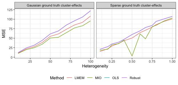
Figure 2: Predictive MSE of the four algorithms in a high dimensional setup (14 clusters, 35 covariates, 50 observations per cluster), where the cluster-effects are truly Gaussian (left) and truly sparse (right)

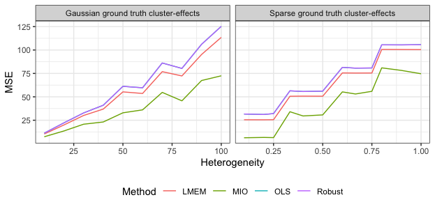
Figure A1: Predictive MSE of the four algorithms in a low dimensional setup (4 clusters, 10 covariates, 50 observations per cluster), where the cluster-effects are truly Gaussian (left) and truly sparse (right)

Another important characteristic of our method is its efficacy as a predictive tool. As we elucidate in the methods section, our procedure leverages the clustered nature of the data, using classification trees, to provide insight into new data points. We compare the predictive performances of these algorithms by looking at the mean-squared error of prediction in a held-out test set, under all the previously mentioned simulation setups. Figure 2 shows that the predictive MSE of the MIO method is clearly lower than that of the other methods in the Gaussian case, and has generally better performance in the sparse case, for all the scenarios under the “High” dimensional setup. A similar trend was observed in “Low” and “Medium” dimensions, with MIO performing uniformly better than the other algorithms. (Appendix Figures A1, A2). Hence, unlike LMEM, our approach can leverage the estimated $\gamma_{k}$s to achieve more accurate cluster-informed predictions

4 Real data example

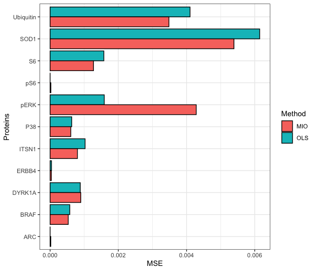
Figure 3: Predictive performance of MIO and OLS on significant proteins from Higuera et al. (2015). LMEM does not produce any results due to convergence issues.

We use the following dataset on Mouse Protein Expression Data from the UCI Machine Learning Repository (Dua & Graff (2017); Ahmed, Dhanasekaran, Block, Tong, Costa, Stasko, and Gardiner (2015)). The data consists of 77 protein measurements from the brains of 72 mice. Among these mice, 38 are control mice and 34 are trisomic mice (that is they are afflicted with Down Syndrome). For each mouse, each protein is measured 15 times. It would be of merit to assume some form of cluster structure within the repeated observations of each of the mice, keeping aside the different classes mentioned in the dataset.

Higuera, Gardiner, and Cios (2015) investigates the proteins that are significant for the differences in classes. As the class dependence does not change between observations of the same mouse, it is safe to assume that there is a level of cluster effect on the expression of these significant proteins. Thus, in order to compare the efficacy of our algorithm against the preexisting methods, we can formulate a linear regression problem using these significant proteins, and see if accounting for the clustering improves our predictions.

Higuera et al. (2015) notes 11 proteins to be significant for distinguishing between at least two of the different classes of mice, among trisomic and control mice. We will be using the 11 proteins for our analysis. These proteins also represent a diverse set of biological pathways, as given in Table 3 of Higuera et al. (2015).

Using complete cases ($n=552$), we train a regression model on each of the proteins above, using the remaining 76 proteins as covariates, and check the predictive performance on a held-out test dataset. Figure 3 shows the predictive performances of the different approaches.

It should be noted that the LMEM approach does not converge in this setup, due to issues in backsolving singularities in data that arise when making distributional assumptions. We can however see that for 7 out of the 11 proteins, there is an improvement of predictive performance between OLS (no clusters assumed) and our cluser-informed MIO approach; this allows us to postulate that there is indeed inherent cluster structure to the data, that can be leveraged for improved regression analysis. In this scenario, LMEM simply isn’t able to model this clustered nature, which demonstrates a pitfall of having a distribution based model for dealing with data, as we require “well-behaved” data for models like LMEM to be able to perform.

5 Discussion

5.1 Comparative performance

Our goal was to construct an algorithm that would be able to work as tool for both inference and prognostication. Testing inferential capabilities involved setting up simulation studies, where we tested over a variety of underlying data generation schemes.

From an inferential perspective, there were two key targets of interest: the regression coefficients $\beta$ and the random effects $\gamma$. In the case of $\beta$ recovery, our algorithm works very well, even when the underlying generation process does not match the MIO process. This is potentially indicative of the effect of dependence between the cluster effects and the covariates, which detracts from other inferential targets in the case of LMEM. In the case of $\gamma$ recovery, our algorithm works quite well, when the random effects are of higher sparsity or lower variance. This is to be expected as extremely low sparsity or high variance muddles the model, and simple sparsity constraints cannot compete with overarching distributional assumptions. Additionally, we have a flexible framework for recovery of the underlying sparsity, since the sparsity hyperparameter is chosen using a validation set. This leads to satisfactory inference on the intra-cluster correlation, which captures the extent of correlation between observations due to their clustering.

Now, from a predictive perspective, we were able to do simulation studies, and apply the algorithms to a real world dataset for testing. We see that our method performs uniformly better than the other methods listed, further cementing the necessity for cluster informed predictions.

5.2 Interpretability

A key philosophy that motivated our approach is the importance of interpretability. From an applied perspective, it is important to know what are the underlying effects that different clusters have, or how an observation’s covariates determine their cluster. Through the framework of observation-wise cluster recovery and interpretable classification trees, we have a way of obtaining this vital information.

Additionally, there is some flexibility in how much interpretability one requires, at the cost of predictive or inferential accuracy. For example, if the main motivating question for an application of this algorithm is the cluster assignment of new observations, then the complexity of the underlying classification tree can be altered to allow for more understandable results. Whereas, if the main motivating question is the prediction of an outcome for a new observations, we could potentially forego interpretable classification trees for stronger classification algorithms such as Random Forests and XGBoost. However, preserving the core philosophy, our algorithm has been designed around algorithms like CARTs or OCTs, to allow for a direct applicative significance, and understandable results.

5.3 Regression extensibility

An overwhelming strength of this optimization approach is the ability to incorporate additional regression constraints seamlessly into the model, since the MIO formulation can be extended to describe many more constraints. For example, using more involved MIO setup, we can control the sparsity and robustness of $\beta$, explicitly control for multicollinearity, and also introduce regularized non-linear effects. We have therefore designed a method that connects hierarchical models - that are ubiquitous in healthcare and economics - to the exciting new field of “holistic” regression (Bertsimas & Li, 2020).

5.4 Outlier detection

A potential side-effect of our model is that it can be leveraged as a tool for outlier detection. Considering a case where each cluster has exactly one observation, and setting a sparsity limit of $\tau\%$, the model would return the trimmed regression coefficient with $(100-\tau)\%$ inlier points. Works such as Chin, Kee, Eriksson, and Neumann (2016),Gómez (2021) and Jammal have formalized forms of outlier detection using mixed-integer optimization. Thus, our method acts potentially as an extension of the methods described in these papers.

5.5 Future work

A base assumption that the cluster-based methods is the knowledge of cluster labels for the training set. One natural extension would be to account for clustering in the training set, without explicit cluster assignments. A two-stage procedure of clustering followed by cluster-based regression may be helpful, but an interesting problem would be to simultaneously solve for the classification tree and MIO regression in order to get cluster assignments and regression estimates at the same time. Additionally, from an inferential perspective, we would like to look into bootstrapping techniques to allow for uncertainty quantification for the causal effects.

5.6 Code availability

The codebase for this project was written using R and Julia and will be available on GitHub. The repository will contain code for:

• simulator for data-generation processes

• code to evaluate performance of methods on the simulated data and the protein expression dataset

• core functions for running our MIO model on the reader’s own data

Appendix A Appendix

True sparsity in $\gamma_{k}$	$||\beta_{\text{true}}-\widehat{\beta}_{OLS}||_{2}^{2}$	$||\beta_{\text{true}}-\widehat{\beta}_{RR}||_{2}^{2}$	$||\beta_{\text{true}}-\widehat{\beta}_{LME}||_{2}^{2}$	$||\beta_{\text{true}}-\widehat{\beta}_{MIO}||_{2}^{2}$
90%	0.23564	0.23553	0.00122	0.00054
80%	0.23334	0.23319	0.001156	0.00055
75%	0.23536	0.23523	0.001213	0.00052
66%	0.10705	0.10702	0.00056	0.00024
60%	0.10894	0.10892	0.00060	0.00028
50%	0.10477	0.10476	0.00061	0.00029
40%	0.07245	0.07244	0.00038	0.00019
33%	0.07114	0.07113	0.00036	0.00018
25%	0.07129	0.07127	0.00035	0.00018
20%	0.04846	0.04845	0.00025	0.00013
10%	0.05316	0.05315	0.00030	0.00014
0%	0.05406	0.05405	0.00024	0.00013

Table A1: Beta recovery under the simulation scenarios where the cluster-effects are truly sparse, with low dimensionality (4 clusters, 10 covariates, 50 observations per cluster)

True sparsity in $\gamma_{k}$	$||\beta_{\text{true}}-\widehat{\beta}_{OLS}||_{2}^{2}$	$||\beta_{\text{true}}-\widehat{\beta}_{RR}||_{2}^{2}$	$||\beta_{\text{true}}-\widehat{\beta}_{LME}||_{2}^{2}$	$||\beta_{\text{true}}-\widehat{\beta}_{MIO}||_{2}^{2}$
90%	0.59369	0.59325	0.00402	0.00143
80%	0.28198	0.28180	0.00159	0.00069
75%	0.18567	0.18562	0.00099	0.00045
66%	0.13559	0.13558	0.00073	0.00034
60%	0.14095	0.14094	0.00071	0.00035
50%	0.11050	0.11050	0.00056	0.00026
40%	0.09078	0.09070	0.00045	0.00022
33%	0.07682	0.07677	0.00038	0.00018
25%	0.06779	0.06780	0.00034	0.00017
20%	0.06986	0.06986	0.00034	0.00016
10%	0.05724	0.05727	0.00029	0.00014
0%	0.05325	0.05322	0.00027	0.00014

Table A2: Beta recovery under the simulation scenarios where the cluster-effects are truly sparse, with medium dimensionality (10 clusters, 25 covariates, 50 observations per cluster)

True sparsity in $\gamma_{k}$	$||\gamma_{\text{true}}-\widehat{\gamma}_{LME}||_{2}^{2}$	$||\gamma_{\text{true}}-\widehat{\gamma}_{MIO}||_{2}^{2}$
90%	0.03988	0.02347
80%	0.04573	0.02194
75%	0.04849	0.02554
66%	0.04519	0.03990
60%	0.04687	0.03587
50%	0.04173	0.04027
40%	0.05245	0.04295
33%	0.04680	0.04445
25%	0.05033	0.04175
20%	0.04401	0.05061
10%	0.03825	0.05017
0%	0.04061	0.05236

Table A3: Gamma recovery for cluster-based methods under the simulation scenarios where the cluster-effects are truly sparse, with low dimensionality (4 clusters, 10 covariates, 50 observations per cluster)

True sparsity in $\gamma_{k}$	$||\gamma_{\text{true}}-\widehat{\gamma}_{LME}||_{2}^{2}$	$||\gamma_{\text{true}}-\widehat{\gamma}_{MIO}||_{2}^{2}$
90%	0.11046	0.03191
80%	0.09521	0.05322
75%	0.10700	0.06776
66%	0.10952	0.07681
60%	0.10673	0.07519
50%	0.10657	0.08277
40%	0.11001	0.10667
33%	0.10921	0.10074
25%	0.10388	0.09744
20%	0.10748	0.12749
10%	0.10500	0.14658
0%	0.12681	0.14561

Table A4: Gamma recovery for cluster-based methods under the simulation scenarios where the cluster-effects are truly sparse, with medium dimensionality (10 clusters, 25 covariates, 50 observations per cluster)

True sparsity in $\gamma_{k}$	Low	Medium	High
90%	79%	82%	86%
80%	70%	71%	79%
75%	60%	65%	72%
66%	57%	59%	63%
60%	49%	53%	58%
50%	41%	43%	45%
40%	38%	33%	39%
33%	25%	25%	31%
25%	15%	15%	20%
20%	11%	14%	15%
10%	0%	6%	8%
0%	0%	0%	0%

Table A5: Sparsity recovery of Gamma of the MIO approach under the different dimensional setups

Variance of $\gamma_{k}$	$||\beta_{\text{true}}-\widehat{\beta}_{OLS}||_{2}^{2}$	$||\beta_{\text{true}}-\widehat{\beta}_{RR}||_{2}^{2}$	$||\beta_{\text{true}}-\widehat{\beta}_{LME}||_{2}^{2}$	$||\beta_{\text{true}}-\widehat{\beta}_{MIO}||_{2}^{2}$
10.0	0.09206	0.09195	0.00378	0.00175
20.0	0.10171	0.10161	0.00199	0.00089
30.0	0.10263	0.10258	0.00132	0.00072
40.0	0.10711	0.10704	0.00134	0.00061
50.0	0.09984	0.09979	0.00094	0.00047
60.0	0.10761	0.10755	0.00111	0.00052
70.0	0.11339	0.11337	0.00060	0.00027
80.0	0.10867	0.10864	0.00069	0.00031
90.0	0.10310	0.10308	0.00049	0.00026
100.0	0.10034	0.10033	0.00045	0.00020

Table A6: Beta recovery under the simulation scenarios where the cluster-effects are truly Gaussian, with low dimensionality (4 clusters, 10 covariates, 50 observations per cluster)

Variance of $\gamma_{k}$	$||\beta_{\text{true}}-\widehat{\beta}_{OLS}||_{2}^{2}$	$||\beta_{\text{true}}-\widehat{\beta}_{RR}||_{2}^{2}$	$||\beta_{\text{true}}-\widehat{\beta}_{LME}||_{2}^{2}$	$||\beta_{\text{true}}-\widehat{\beta}_{MIO}||_{2}^{2}$
10.0	0.11150	0.11145	0.00289	0.00142
20.0	0.12713	0.12709	0.00161	0.00074
30.0	0.11915	0.11911	0.00116	0.00056
40.0	0.13113	0.13112	0.00094	0.00043
50.0	0.12789	0.12787	0.00068	0.00034
60.0	0.11203	0.11205	0.00061	0.00029
70.0	0.12111	0.12116	0.00045	0.00020
80.0	0.13204	0.13202	0.00042	0.00020
90.0	0.12829	0.12825	0.00042	0.00020
100.0	0.13437	0.13436	0.00035	0.00016

Table A7: Beta recovery under the simulation scenarios where the cluster-effects are truly Gaussian, with medium dimensionality (10 clusters, 25 covariates, 50 observations per cluster)

Variance of $\gamma_{k}$	$||\gamma_{\text{true}}-\widehat{\gamma}_{LMEM}||_{2}^{2}$	$||\gamma_{\text{true}}-\widehat{\gamma}_{MIO}||_{2}^{2}$
10.0	0.04014	0.02846
20.0	0.04251	0.02961
30.0	0.04119	0.03812
40.0	0.04579	0.04118
50.0	0.03857	0.04495
60.0	0.04116	0.04400
70.0	0.04085	0.05030
80.0	0.03746	0.05121
90.0	0.04510	0.06128
100.0	0.04305	0.06324

Table A8: Gamma recovery for cluster-based methods under the simulation scenarios where the cluster-effects are truly Gaussian, with low dimensionality (4 clusters, 10 covariates, 50 observations per cluster)

Variance of $\gamma_{k}$	$||\gamma_{\text{true}}-\widehat{\gamma}_{LMEM}||_{2}^{2}$	$||\gamma_{\text{true}}-\widehat{\gamma}_{MIO}||_{2}^{2}$
10.0	0.10519	0.07696
20.0	0.09958	0.09785
30.0	0.10009	0.08733
40.0	0.10931	0.10110
50.0	0.10460	0.11122
60.0	0.09965	0.11120
70.0	0.10389	0.13616
80.0	0.10631	0.14843
90.0	0.10476	0.15833
100.0	0.10682	0.16284

Table A9: Gamma recovery for cluster-based methods under the simulation scenarios where the cluster-effects are truly Gaussian, with medium dimensionality (10 clusters, 25 covariates, 50 observations per cluster)

True ICC	$||\beta_{\text{true}}-\widehat{\beta}_{LMEM}||_{2}^{2}$	$||\beta_{\text{true}}-\widehat{\beta}_{MIO}||_{2}^{2}$
10%	8%	4%
20%	18%	13%
30%	29%	25%
40%	39%	39%
50%	49%	48%
60%	59%	59%
70%	70%	69%
80%	80%	79%
90%	90%	90%

Table A10: Comparison of ICC recovery in Medium dimensionality (10 clusters, 25 covariates, 50 observations per cluster) between LMEM and MIO

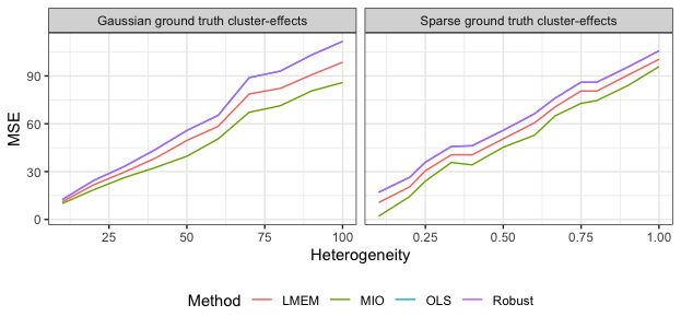
Figure A2: Predictive MSE of the four algorithms in a medium dimensional setup (10 clusters, 25 covariates, 50 observations per cluster), where the cluster-effects are truly Gaussian (left) and truly sparse (right)

References

- Ahmed et al. (2015) Ahmed, M. M., Dhanasekaran, A. R., Block, A., Tong, S., Costa, A. C. S., Stasko, M., and Gardiner, K. J. Protein dynamics associated with failed and rescued learning in the ts65dn mouse model of down syndrome. PLOS ONE, 10(3):e0119491, Mar 2015. ISSN 1932-6203. doi: 10.1371/journal.pone.0119491.
- Balasankar et al. (2021) Balasankar, V., Varma Penumatsa, S. S., and Pandu Ranga Vital, T. Empirical statistical analysis and cluster studies on socio-economic status (ses) dataset. IOP Conference Series: Materials Science and Engineering, 1085(1):012030, Feb 2021. ISSN 1757-8981, 1757-899X. doi: 10.1088/1757-899X/1085/1/012030.
- Bartko (1966) Bartko, J. J. The intraclass correlation coefficient as a measure of reliability. Psychol. Rep., 19(1):3–11, August 1966.
- Bertsimas & Dunn (2017) Bertsimas, D. and Dunn, J. Optimal classification trees. Machine Learning, 106(7):1039–1082, Jul 2017. ISSN 0885-6125, 1573-0565. doi: 10.1007/s10994-017-5633-9.
- Bertsimas & Li (2020) Bertsimas, D. and Li, M. L. Scalable holistic linear regression. Operations Research Letters, 48(3):203–208, May 2020. ISSN 01676377. doi: 10.1016/j.orl.2020.02.008. arXiv:1902.03272 [cs, math, stat].
- Bertsimas et al. (2015) Bertsimas, D., King, A., and Mazumder, R. Best subset selection via a modern optimization lens. (arXiv:1507.03133), Jul 2015. URL http://arxiv.org/abs/1507.03133. arXiv:1507.03133 [math, stat].
- Bradley & Taqqu (2003) Bradley, B. O. and Taqqu, M. S. Financial Risk and Heavy Tails, pp. 35–103. Elsevier, 2003. ISBN 978-0-444-50896-6. doi: 10.1016/B978-044450896-6.50004-2. URL https://linkinghub.elsevier.com/retrieve/pii/B9780444508966500042.
- Breiman et al. (2017) Breiman, L., Friedman, J. H., Olshen, R. A., and Stone, C. J. Classification and regression trees. Routledge, 2017.
- Chin et al. (2016) Chin, T.-J., Kee, Y. H., Eriksson, A., and Neumann, F. Guaranteed outlier removal with mixed integer linear programs. In 2016 IEEE Conference on Computer Vision and Pattern Recognition (CVPR), pp. 5858–5866, Las Vegas, NV, Jun 2016. IEEE. ISBN 978-1-4673-8851-1. doi: 10.1109/CVPR.2016.631. URL https://ieeexplore.ieee.org/document/7781000/.
- Desai & Begg (2008) Desai, M. and Begg, M. D. A comparison of regression approaches for analyzing clustered data. American Journal of Public Health, 98(8):1425–1429, Aug 2008. ISSN 0090-0036, 1541-0048. doi: 10.2105/AJPH.2006.108233.
- Dua & Graff (2017) Dua, D. and Graff, C. UCI machine learning repository, 2017. URL http://archive.ics.uci.edu/ml.
- Duran & Grossmann (1986) Duran, M. A. and Grossmann, I. E. An outer-approximation algorithm for a class of mixed-integer nonlinear programs. Mathematical programming, 36:307–339, 1986.
- Graubard & Korn (1994) Graubard, B. I. and Korn, E. L. Regression analysis with clustered data. Statistics in Medicine, 13(5–7):509–522, Mar 1994. ISSN 02776715, 10970258. doi: 10.1002/sim.4780130514.
- Gurobi Optimization, LLC (2023) Gurobi Optimization, LLC. Gurobi Optimizer Reference Manual, 2023. URL https://www.gurobi.com.
- Gómez (2021) Gómez, A. Outlier detection in time series via mixed-integer conic quadratic optimization. SIAM Journal on Optimization, 31(3):1897–1925, Jan 2021. ISSN 1052-6234, 1095-7189. doi: 10.1137/19M1306233.
- Higuera et al. (2015) Higuera, C., Gardiner, K. J., and Cios, K. J. Self-organizing feature maps identify proteins critical to learning in a mouse model of down syndrome. PLOS ONE, 10(6):e0129126, Jun 2015. ISSN 1932-6203. doi: 10.1371/journal.pone.0129126.
- (17) Jammal, M. Variable selection and outlier detection viamixed integer programming.
- Laird & Ware (1982) Laird, N. M. and Ware, J. H. Random-effects models for longitudinal data. 1982.
- Liao et al. (2016) Liao, M., Li, Y., Kianifard, F., Obi, E., and Arcona, S. Cluster analysis and its application to healthcare claims data: a study of end-stage renal disease patients who initiated hemodialysis. BMC Nephrol., 17(1):25, March 2016.
- Liu & Pierce (1994) Liu, Q. and Pierce, D. A. A note on Gauss-Hermite quadrature. Biometrika, 81(3):624, August 1994.
- Mancl & Leroux (1996) Mancl, L. A. and Leroux, B. G. Efficiency of regression estimates for clustered data. Biometrics, 52(2):500, Jun 1996. ISSN 0006341X. doi: 10.2307/2532890.
- McNeish (2014) McNeish, D. M. Analyzing clustered data with ols regression: The effect of a hierarchical data structure. 40, 2014.
- Ntani et al. (2021) Ntani, G., Inskip, H., Osmond, C., and Coggon, D. Consequences of ignoring clustering in linear regression. BMC Medical Research Methodology, 21(1):139, Dec 2021. ISSN 1471-2288. doi: 10.1186/s12874-021-01333-7.
- She (2010) She, Y. Sparse regression with exact clustering. Electronic Journal of Statistics, 4(none), Jan 2010. ISSN 1935-7524. doi: 10.1214/10-EJS578. URL https://projecteuclid.org/journals/electronic-journal-of-statistics/volume-4/issue-none/Sparse-regression-with-exact-clustering/10.1214/10-EJS578.full.
- Shiratori et al. (2020) Shiratori, T., Kobayashi, K., and Takano, Y. Prediction of hierarchical time series using structured regularization and its application to artificial neural networks. PLoS One, 15(11):e0242099, November 2020.
- Welham et al. (2004) Welham, S., Cullis, B., Gogel, B., Gilmour, A., and Thompson, R. Prediction in linear mixed models. Australian & New Zealand Journal of Statistics, 46(3):325–347, Sep 2004. ISSN 1369-1473, 1467-842X. doi: 10.1111/j.1467-842X.2004.00334.x.
- Wooldridge & Zhu (2020) Wooldridge, J. M. and Zhu, Y. Inference in approximately sparse correlated random effects probit models with panel data. Journal of Business & Economic Statistics, 38(1):1–18, Jan 2020. ISSN 0735-0015, 1537-2707. doi: 10.1080/07350015.2019.1681276.