Convergence rates of a discrete feedback control arising in mean-field linear quadratic optimal control problems

Abstract

In this work, we propose a feedback control based temporal discretization for linear quadratic optimal control problems (LQ problems) governed by controlled mean-field stochastic differential equations. We firstly decompose the original problem into two problems: a stochastic LQ problem and a deterministic one. Secondly, we discretize both LQ problems one after another relying on Riccati equations and control’s feedback representations. Then, we prove the convergence rates for the proposed discretization and present an effective algorithm. Finally, a numerical example is provided to support the theoretical finding.

Keywords: Convergence rate, mean-field linear quadratic optimal control problem, closed–loop optimal control strategy, Riccati equation

AMS 2010 subject classification: 93E20, 49N10, 93B52

1 Introduction

The present work is concerned with the numerical scheme for the linear quadratic optimal control problems (LQ problems, for short) governed by controlled mean-field stochastic differential equations (MF-SDEs, for short), which are special stochastic optimal control problems.

In 1938, the idea of mean field interaction in mathematical physics was proposed by Vlasov. From 1950s, a kind of MF-SDEs, named by McKean-Vlasov SDEs, was proposed and then systematically studied. Up to now, theory of MF-SDEs has significant impact in several areas such as physics, financial mathematics, stochastic optimal control, social interactions.

As three well-recognized fundamental results of stochastic optimal control theory, Pontryagin-type maximum principle (MP, for short) (see, e.g., [9, 26]), Bellman dynamic programming principle (DPP, for short) (see, e.g., [7, 12, 27]) and LQ theory (see, e.g., [22, 23]) have been established in the past half century. For the stochastic optimal control problems subject to MF-SDEs, there still exists some works; see, e.g., [1, 11, 3, 25, 33, 21, 24].

However, general stochastic optimal control problems, except for some special case such as one-dimensional state equation, can not admit explicitly closed form solutions. Therefore, effective numerical schemes for these problems are necessary, and attract some attentions. Up to now, there are two widely applied and popular approaches to numerically solve stochastic optimal control problems: DPP based approach and MP based one. The first approach relies on DPP and Hamilton-Jacobi-Bellman (HJB, for short) equation. By establishing the bridge between the original problem and an HJB equation, then numerically solving the HJB equation, one can obtain an approximation of the optimal control (see, e.g., [16, 17, 6]). However, due to the nonlinearity of the HJB equation, this approach is computational expensive. For the second approach, thanks to MP, the optimal pair satisfies a coupled forward-backward stochastic differential equation (FBSDE, for short). The difficulty and complexity of the second approach stem from the fact that this equation is coupled and the solution to this equation should be adapted. To decouple this FBSDE, a (stochastic) gradient descent algorithm can be adopted (see, e.g., [14, 4, 5, 28, 29]). Besides, gradient projection methods for stochastic optimal control problems with deterministic control variables are also proposed; see [13, 19]. To guarantee the solution’s adaptivity, conditional expectations are introduced (see, e.g., [35, 8]). Although there exists numerous works to simulate conditional expectations (see, e.g., [18, 8, 20, 30, 10]), the study of computation on conditional expectations is far from mature till now. From this perspective, the computational cost of MP based approach is high.

To reduce the computation cost, recently based on LQ theory, Riccati based schemes for LQ problems subject to controlled SDEs are proposed in [32]. Avoiding solving coupled equations and simulating conditional expectations, these schemes can greatly save computation time.

In this work, adopting LQ theory of MF-SDEs and Riccati equations, we aim at proposing an efficient algorithm with convergence rates to solve LQ problems governed by MF-SDEs, which will be called MF-LQ problems. To be specific, Let $(\Omega,{\mathcal{F}},{\mathbb{F}},{\mathbb{P}})$ be a complete filtered probability space on which a standard one-dimensional Brownian motion $W=\{W(t):\,t\geq 0\}$ is defined, where $\mathbb{F}=\{{\cal F}_{t}\}_{t\geq 0}$ is the natural filtration of $W$ augmented by all the $\mathbb{P}$-null sets in ${\cal F}$. Consider the following cost functional

$${\cal J}(u(\cdot)) =\mathbb{E}\Big{[}\int_{0}^{T}\big{(}\langle Qx(t),x(t)\rangle+\langle\bar{Q}\mathbb{E}[x(t)],\mathbb{E}[x(t)]\rangle+\langle Ru(t),u(t)\rangle+\langle\bar{R}\mathbb{E}[u(t)],\mathbb{E}[u(t)]\rangle\big{)}\,\mathrm{d}t$$

$$\quad+\langle Gx(T),x(T)\rangle+\langle\bar{G}\mathbb{E}[x(T)],\mathbb{E}[x(T)]\rangle\Big{]}$$

subject to a controlled MF-SDE:

$$\left\{\begin{aligned} &\,\mathrm{d}x(t)=\left(Ax(t)+\bar{A}\mathbb{E}[x(t)]+Bu(t)+\bar{B}\mathbb{E}[u(t)]\right)\,\mathrm{d}t\\ &\qquad\qquad+\left(Cx(t)+\bar{C}\mathbb{E}[x(t)]+Du(t)+\bar{D}\mathbb{E}[u(t)]\right)\,\mathrm{d}W(t)\quad&\forall\,t\in[0,T]\,,\\ &x(0)=x_{0}\in\mathbb{R}^{n}\,,\end{aligned}\right.$$ (1.1)

where $A,\,\bar{A},\,C,\,\bar{C},\,Q,\,\bar{Q},\,G,\,\bar{G}\in\mathbb{R}^{n\times n}$, $B,\,\bar{B},\,D,\,\bar{D}\in\mathbb{R}^{n\times m}$, $R,\,\bar{R}\in\mathbb{R}^{m\times m}$, and $u(\cdot)$ is the control variable. The space of admissible controls for (1.1) is

$$L^{2}_{\mathbb{F}}(0,T;\mathbb{R}^{m})\triangleq\Big{\{}\varphi:(0,T)\times\Omega\to\mathbb{R}^{m}\,\big{|}\,\varphi(\cdot)\hbox{ is $\mathbb{F}$-adapted and }\int_{0}^{T}\mathbb{E}[\|\varphi(t)\|^{2}]\,\mathrm{d}t<\infty\Big{\}}\,.$$

The considered MF-LQ problem can be stated as follows.
Problem (MF-LQ). For given $x_{0}\in\mathbb{R}^{n}$, find an optimal control $u^{*}(\cdot)\in L^{2}_{\mathbb{F}}(0,T;\mathbb{R}^{m})$ such that

$${\cal J}(u^{*}(\cdot))=\inf_{u(\cdot)\in L^{2}_{\mathbb{F}}(0,T;\mathbb{R}^{m})}{\cal J}(u(\cdot))\,.$$

Our goal is to numerically approximate the optimal stochastic control $u^{*}(\cdot)$ of Problem (MF-LQ).

The main strategy for discretization of Problem (MF-LQ) is as follows: Firstly, thanks to the optimal control’s state feedback form and two corresponding differential Riccati equations, we introduce a stochastic LQ problem, Problem (LQ)^1,t, related to the first Riccati equation, and a discrete stochastic LQ problem, Problem (LQ)${}^{1,t}_{\tau}$, to approximate Problem (LQ)^1,t; Secondly, relying on the solution to the first aforementioned differential Riccati equation, we introduce a deterministic LQ problem, Problem (LQ)^2,t, and its temporal discretization, Problem (LQ)${}_{\tau}^{2,t}$, whose related difference Riccati equation is proved to converge to the solution of the second aforementioned differential Riccati equation; Thirdly, by inverting the above two steps and adopting the optimal controls’ state feedback representations of the above four auxiliary LQ problems, we can propose a discretization for Problem (MF-LQ), prove the convergence of our proposed discretization and derive the rates of convergence. This is one contribution of this work.

As an application of our scheme, we actually can propose efficient and accurate algorithms with rates to numerically solve differential Riccati equations and a family of coupled mean-field forward-backward stochastic differential equations. This is another contribution of this work.

The rest of this paper is organized as follows. In Section 2, we introduce some notations, review results on solvability of Problem (MF-LQ), present temporal discretization of stochastic LQ problems and their corresponding Riccati equations, and state the convergence with rates for aforementioned discretization of Riccati equation which is related to the optimal control’s state feedback representation. In Section 3, by virtue of closed–loop optimal control strategy, we prove the convergence rates of temporal discretization for Problem (MF-LQ), and propose an accurate and efficient algorithm, as well as carry out an example to verify our theoretical results.

2 Preliminaries

2.1 Notations and solvability of Problem (MF-LQ)

Let $\mathbb{K}$ be $\mathbb{R}^{n}$ or $\mathbb{R}^{m}$. Denote by $L^{2}_{\mathbb{F}}(0,T;\mathbb{K})$ the space of $\mathbb{K}$-valued, $\mathbb{F}$-adapted processes $\varphi(\cdot)$ satisfying $\mathbb{E}\big{[}\int_{0}^{T}\|\varphi(t)\|_{\mathbb{K}}^{2}\,\mathrm{d}t\big{]}<\infty$; by $L^{2}_{\mathbb{F}}(\Omega;C([0,T];\mathbb{K}))$ the subspace of $L^{2}_{\mathbb{F}}(0,T;\mathbb{K})$, such that every element $\varphi(\cdot)$ has a continuous path and satisfies $\mathbb{E}\big{[}\sup_{t\in[0,T]}\|\varphi(t)\|_{\mathbb{K}}^{2}\big{]}<\infty$; by $L^{2}(0,T;\mathbb{K})$ the space of $\mathbb{K}$-valued functions $\varphi(\cdot)$ satisfying $\int_{0}^{T}\|\varphi(t)\|_{\mathbb{K}}^{2}\,\mathrm{d}t<\infty$. For any matrix $M$, denote $\|M\|\triangleq\sqrt{\rho(M^{\top}M)}$, where $\rho$ represents the spectral radius. A symmetric matrix $M>0(\geq 0)$ means that it is positive definite (positive semi-definite). Denote by $I_{n}$ the identity matrix of size $n$.

We denote by $I_{\tau}=\{t_{n}\}_{n=0}^{N}\subset[0,T]$ a time mesh with maximum step size $\tau:=\max\{t_{n+1}-t_{n}:\,n=0,1,\cdots,N-1\}$, and $\Delta_{n}W=W(t_{n})-W(t_{n-1})$ for all $n=1,\cdots,N$. For a given time mesh $I_{\tau}$, we can define $\nu:[0,T]\to I_{\tau}$ by

$$\nu(t)=t_{k}\qquad\forall\,t\in[t_{k},t_{k+1}),\,k=0,1,\cdots,N-1\,.$$ (2.1)

For simplicity, we choose a uniform partition, i.e. step-size $\tau=T/N$ and $\tau\leq 1$. Denote by ${\cal C}$ a generic positive constant independent of data and $I_{\tau}$, which may vary from one place to another.

Throughout this paper, to guarantee the solvability of Problem (MF-LQ), we make the following assumption.
(A) $Q\geq 0,\,Q+\bar{Q}\geq 0,\,G\geq 0,\,G+\bar{G}\geq 0,\,R>0,\,R+\bar{R}>0$.

For simplicity, denote $\widehat{\varphi}\triangleq\varphi+\bar{\varphi}$, for $\varphi=A,\,B,\,C,\,D,\,Q,\,R,\,G$.

The results in this work can be extended to cases with a higher-dimensional $W(\cdot)$, a general partition $I_{\tau}$, and/or time-varying deterministic coefficients without significant difficulties. Note that for the time-varying coefficients, the assumption should be changed to the following:
(A1) $Q(\cdot)\geq 0,\,\widehat{Q}(\cdot)\geq 0,\,G\geq 0,\,\widehat{G}\geq 0,\,R(\cdot)-\delta I_{m}\geq 0,\,\widehat{R}(\cdot)-\delta I_{m}\geq 0$, where $\delta$ is a positive constant;
(A2) $\varphi(\cdot),\,\bar{\varphi}(\cdot)$ are Lipchitz continuous, for $\varphi(\cdot)=A(\cdot),\,B(\cdot),\,C(\cdot),\,D(\cdot),\,Q(\cdot),\,R(\cdot)$.

The following result is on the regularity of the state $x(\cdot)$; see [33, Proposition 2.6].

    Lemma 2.1.

Let (A) hold. Then for any $(x_{0},u(\cdot))\in\mathbb{R}^{n}\times L^{2}_{\mathbb{F}}(0,T;\mathbb{R}^{m})$, equation (1.1) admits a unique solution $x(\cdot)\in L^{2}_{\mathbb{F}}(\Omega;C([0,T];\mathbb{R}^{n}))$.

The following result states Pontryagin-type maximum principles for Problem (MF-LQ), which guarantees solvability of Problem (MF-LQ). The reader can refer to [33, Proposition 2.8, Theorems 3.1 & 3.2].

    Lemma 2.2.

Under the assumption (A), Problem (MF-LQ) admits a unique optimal pair $(x^{*}(\cdot),u^{*}(\cdot))\in L^{2}_{\mathbb{F}}(0,T;\mathbb{R}^{n})\times L_{\mathbb{F}}^{2}(0,T;\mathbb{R}^{m})$, and the unique solvability of Problem (MF-LQ) is equivalent to the unique solvability of the following equation:

$$\left\{\begin{aligned} &\,\mathrm{d}x^{*}(t)=\left(Ax^{*}(t)+\bar{A}\mathbb{E}[x^{*}(t)]+Bu^{*}(t)+\bar{B}\mathbb{E}[u^{*}(t)]\right)\,\mathrm{d}t\\ &\qquad\qquad+\left(Cx^{*}(t)+\bar{C}\mathbb{E}[x^{*}(t)]+Du^{*}(t)+\bar{D}\mathbb{E}[u^{*}(t)]\right)\,\mathrm{d}W(t)\qquad\forall\,t\in[0,T]\,,\\ &\,\mathrm{d}y(t)=-\big{(}A^{\top}y(t)+\bar{A}^{\top}\mathbb{E}[y(t)]+C^{\top}z(t)+\bar{C}^{\top}\mathbb{E}[z(t)]-Qx^{*}(t)-\bar{Q}\mathbb{E}[x^{*}(t)]\big{)}\,\mathrm{d}t\\ &\qquad\qquad+z(t)\,\mathrm{d}W(t)\qquad\forall\,t\in[0,T]\,,\\ &x^{*}(0)=x_{0}\,,\quad y(T)=-Gx^{*}(T)\,,\end{aligned}\right.$$ (2.2)

together with the optimality condition

$$Ru^{*}(\cdot)+\bar{R}\mathbb{E}[u^{*}(\cdot)]-\big{(}B^{\top}y(\cdot)+\bar{B}^{\top}\mathbb{E}[y(\cdot)]+D^{\top}z(\cdot)+\bar{D}^{\top}\mathbb{E}[z(\cdot)]\big{)}=0\quad\hbox{\rm a.e.}$$

In the following, we tend to state the closed–loop optimal control strategy of MF-LQ problems, where two differential Riccati equations are needed. By [33], these two Riccati equations (with time variable suppressed) related to Problem (MF-LQ) read

$$\left\{\begin{aligned} &P^{\prime}+PA+A^{\top}P+C^{\top}PC+Q\\ &\qquad-(B^{\top}P+D^{\top}PC)^{\top}\Sigma_{0}^{-1}(B^{\top}P+D^{\top}PC)=0\quad\mbox{in }[0,T]\,,\\ &P(T)=G\,,\\ \end{aligned}\right.$$ (2.3)

and

$$\left\{\begin{aligned} &\Pi^{\prime}+\Pi\widehat{A}+\widehat{A}^{\top}\Pi+\widehat{C}^{\top}P\widehat{C}+\widehat{Q}\\ &\qquad-(\widehat{B}^{\top}\Pi+\widehat{D}^{\top}P\widehat{C})^{\top}\Sigma_{1}^{-1}(\widehat{B}^{\top}\Pi+\widehat{D}^{\top}P\widehat{C})=0\quad\mbox{in }[0,T]\,,\\ &\Pi(T)=\widehat{G}\,,\\ \end{aligned}\right.$$ (2.4)

where

$$\Sigma_{0}=R+D^{\top}PD\,,\qquad\Sigma_{1}=\widehat{R}+\widehat{D}^{\top}P\widehat{D}\,.$$ (2.5)

The following result on solvability of these two equations and the optimal control’s closed–loop representation belongs to [33, Theorem 4.1].

    Lemma 2.3.

Under the assumption (A), Riccati equations (2.3) and (2.4) admit unique solutions $P(\cdot)$ and $\Pi(\cdot)$ which are positive semi-definite. Further, the optimal control to Problem (MF-LQ) has the following feedback representation (with time variable suppressed):

$$u^{*}=-\Sigma_{0}^{-1}\big{[}B^{\top}P+D^{\top}PC\big{]}(x^{*}-\mathbb{E}[x^{*}])-\Sigma_{1}^{-1}\big{[}\widehat{B}^{\top}\Pi+\widehat{D}^{\top}P\widehat{C}\big{]}\mathbb{E}[x^{*}]\,.$$ (2.6)

2.2 Temporal discretization of parametrized MF-LQ problems

We employ a uniform mesh $I_{\tau}=\{t_{i}\}_{i=0}^{N}$ covering $[0,T]$, and for any $t_{l}\in I_{\tau},\,l=0,1,\cdots,N-1$, consider step size process pair $(x_{\tau}(\cdot),u_{\tau}(\cdot))\in\mathbb{X}_{\tau}(t_{l},T)\times\mathbb{U}_{\tau}(t_{l},T)\subset L^{2}_{\mathbb{F}}(t_{l},T;\mathbb{R}^{n})\times L_{\mathbb{F}}^{2}(t_{l},T;\mathbb{R}^{m})$, where

$$\mathbb{X}_{\tau}(t_{l},T) \triangleq\left\{x(\cdot)\in L^{2}_{\mathbb{F}}(t_{l},T;\mathbb{R}^{n})\,|\,x(t)=x(t_{n}),\,\,\forall t\in[t_{n},t_{n+1}),\,\,n=l,l+1,\cdots,\,N-1\right\}\,,$$

$$\mathbb{U}_{\tau}(t_{l},T) \triangleq\left\{u(\cdot)\in L^{2}_{\mathbb{F}}(t_{l},T;\mathbb{R}^{m})\,|\,u(t)=u(t_{n}),\,\,\forall t\in[t_{n},t_{n+1}),\,\,n=l,l+1,\cdots,\,N-1\right\}\,,$$

and for any $x(\cdot)\in\mathbb{X}_{\tau}(t_{l},T)$ and $u(\cdot)\in\mathbb{U}_{\tau}(t_{l},T)$,

$$\|x(\cdot)\|_{\mathbb{X}_{\tau}(t_{l},T)}\triangleq\Big{(}\tau\sum_{n=l}^{N-1}\mathbb{E}\big{[}\|x(t_{n})\|^{2}\big{]}\Big{)}^{1/2}\,,\quad\mbox{and}\quad\|u(\cdot)\|_{\mathbb{U}_{\tau}(t_{l},T)}\triangleq\Big{(}\tau\sum_{n=l}^{N-1}\mathbb{E}\big{[}\|u(t_{n})\|^{2}\big{]}\Big{)}^{1/2}.$$

We also need the following two deterministic spaces:

$$\bar{\mathbb{X}}_{\tau}(t_{l},T) \triangleq\left\{x(\cdot)\in L^{2}(t_{l},T;\mathbb{R}^{n})\,|\,x(t)=x(t_{n}),\,\,\forall t\in[t_{n},t_{n+1}),\,\,n=l,l+1,\cdots,\,N-1\right\}\,,$$

$$\bar{\mathbb{U}}_{\tau}(t_{l},T) \triangleq\left\{u(\cdot)\in L^{2}(t_{l},T;\mathbb{R}^{m})\,|\,u(t)=u(t_{n}),\,\,\forall t\in[t_{n},t_{n+1}),\,\,n=l,l+1,\cdots,\,N-1\right\}\,,$$

and for any $x(\cdot)\in\bar{\mathbb{X}}_{\tau}(t_{l},T)$ and $u(\cdot)\in\bar{\mathbb{U}}_{\tau}(t_{l},T)$,

$$\|x(\cdot)\|_{\bar{\mathbb{X}}_{\tau}(t_{l},T)}\triangleq\Big{(}\tau\sum_{n=l}^{N-1}\|x(t_{n})\|^{2}\Big{)}^{1/2}\,,\quad\mbox{and}\quad\|u(\cdot)\|_{\bar{\mathbb{U}}_{\tau}(t_{l},T)}\triangleq\Big{(}\tau\sum_{n=l}^{N-1}\|u(t_{n})\|^{2}\Big{)}^{1/2}.$$

For the optimal pair $(x^{*}(\cdot),u^{*}(\cdot))$ of Problem (MF-LQ), by Lemma 2.1, it follows that $x^{*}(\nu(\cdot))\in\mathbb{X}_{\tau}(0,T)$, where $\nu(\cdot)$ is defined in (2.1). Then by Lemma 2.3, we know that $u^{*}(\nu(\cdot))\in\mathbb{U}_{\tau}(0,T)$. By Hölder’s inequality, it is easy to see that for any $(x(\cdot),u(\cdot))\in\mathbb{X}_{\tau}(t_{l},T)\times\mathbb{U}_{\tau}(t_{l},T),l=0,1,\cdots,N-1$, $(\mathbb{E}[x(\cdot)],\mathbb{E}[u(\cdot)])\in\bar{\mathbb{X}}_{\tau}(t_{l},T)\times\bar{\mathbb{U}}_{\tau}(t_{l},T)$.

Now, we introduce parametrized MF-LQ problems. For any $t\in[0,T]$, $l=0,1,\cdots,N-1$, consider the following systems:

$$\left\{\begin{aligned} &\,\mathrm{d}x(s)=\left(Ax(s)+\bar{A}\mathbb{E}[x(s)]+Bu(s)+\bar{B}\mathbb{E}[u(s)]\right)\,\mathrm{d}s\\ &\qquad\qquad+\left(Cx(s)+\bar{C}\mathbb{E}[x(s)]+Du(s)+\bar{D}\mathbb{E}[u(s)]\right)\,\mathrm{d}W(s)\quad&\forall\,s\in[t,T]\,,\\ &x(t)=x_{t}\in\mathbb{R}^{n}\,,\end{aligned}\right.$$ (2.7)

and

$$\left\{\begin{aligned} &x_{\tau}(t_{k+1})-x_{\tau}(t_{k})=\tau\big{[}Ax_{\tau}(t_{k})+\bar{A}\mathbb{E}[x_{\tau}(t_{k})]+Bu_{\tau}(t_{k})+\bar{B}\mathbb{E}[u_{\tau}(t_{k})]\big{]}\\ &\qquad\qquad\qquad\qquad\qquad+\big{[}Cx_{\tau}(t_{k})+\bar{C}\mathbb{E}[x_{\tau}(t_{k})]+Du_{\tau}(t_{k})+\bar{D}\mathbb{E}[u_{\tau}(t_{k})]\big{]}\Delta_{k+1}W\\ &\qquad\qquad\qquad\qquad\qquad\qquad\qquad\qquad\qquad\qquad\quad k=l,l+1,\cdots,N-1\,,\\ &x_{\tau}(t_{l})=x_{t_{l}}\in\mathbb{R}^{n}\,,\end{aligned}\right.$$ (2.8)

as well as the cost functionals

$${\cal J}(t,x_{t};u(\cdot))$$ (2.9)

$$=\mathbb{E}\Big{[}\int_{t}^{T}\big{(}\langle Qx(s),x(s)\rangle+\langle\bar{Q}\mathbb{E}[x(s)],\mathbb{E}[x(s)]\rangle+\langle Ru(s),u(s)\rangle+\langle\bar{R}\mathbb{E}[u(s)],\mathbb{E}[u(s)]\rangle\big{)}\,\mathrm{d}s$$

$$\quad+\langle Gx(T),x(T)\rangle+\langle\bar{G}\mathbb{E}[x(T)],\mathbb{E}[x(T)]\rangle\Big{]}$$

and

$${\cal J}_{\tau}(t_{l},x_{t_{l}};u_{\tau}(\cdot)) =\|\sqrt{Q}x_{\tau}(\cdot)\|^{2}_{\mathbb{X}_{\tau}(t_{l},T)}+\langle\bar{Q}\mathbb{E}[x_{\tau}(\cdot)],\mathbb{E}[x_{\tau}(\cdot)]\rangle_{\bar{\mathbb{X}}_{\tau}(t_{l},T)}$$ (2.10)

$$\quad+\|\sqrt{R}u_{\tau}(\cdot)\|^{2}_{\mathbb{U}_{\tau}(t_{l},T)}+\langle\bar{R}\mathbb{E}[u_{\tau}(\cdot)],\mathbb{E}[u_{\tau}(\cdot)]\rangle_{\bar{\mathbb{U}}_{\tau}(t_{l},T)}$$

$$\quad+\mathbb{E}\langle Gx_{\tau}(T),x_{\tau}(T)\rangle+\langle\bar{G}\mathbb{E}[x_{\tau}(T)],\mathbb{E}[x_{\tau}(T)]\rangle\,.$$

Here, $x_{\tau}(\cdot)$ and $u_{\tau}(\cdot)$ are defined as follows:

$$x_{\tau}(t)=x_{\tau}(t_{k})\,,\quad u_{\tau}(t)=u_{\tau}(t_{k})\qquad\forall\,t\in[t_{k},t_{k}+1),\,k=l,l+1,\cdots,N-1.$$

In the below, we construct two auxiliary LQ problems.
Problem (LQ)^1,t. For given $x_{t}\in\mathbb{R}^{n}$, minimize ${\cal J}(t,x_{t};u(\cdot))$ over $L^{2}_{\mathbb{F}}(t,T;\mathbb{R}^{m})$ subject to (2.7) with $\bar{A}=\bar{C}=\bar{G}=0,\,\bar{B}=\bar{D}=0,\,\bar{R}=0$.
Problem (LQ)${}_{\tau}^{1,t_{l}}$. For given $x_{t_{l}}\in\mathbb{R}^{n}$, minimize ${\cal J}_{\tau}(t_{l},x_{t_{l}};u_{\tau}(\cdot))$ over $\mathbb{U}_{\tau}(t_{l},T)$ subject to (2.8) with $\bar{A}=\bar{C}=\bar{G}=0,\,\bar{B}=\bar{D}=0,\,\bar{R}=0$.

The following result comes from [2, Theorem 4.3].

    Lemma 2.4.

Under the assumption (A), for any $l=0,1,\cdots,N-1$, Problem (LQ)${}_{\tau}^{1,t_{l}}$ admits a unique optimal control $u_{\tau}^{*}(\cdot)$, which has the following feedback representation:

$$u_{\tau}^{*}(t_{k})=-(W_{k}^{1})^{-1}H_{k}^{1}x_{\tau}^{*}(t_{k})\qquad\forall\,k=l,l+1,\cdots,N-1\,,$$ (2.11)

and

$$\inf_{u_{\tau}(\cdot)\in\mathbb{U}_{\tau}(t_{l},T)}{\cal J}_{\tau}(t_{l},x_{t_{l}};u_{\tau}(\cdot))=\langle P_{l}x_{t_{l}},x_{t_{l}}\rangle\,,$$ (2.12)

where

$$W_{k}^{1}=R+B^{\top}P_{k+1}B\tau+D^{\top}P_{k+1}D\,,\qquad H_{k}^{1}=B^{\top}P_{k+1}(I_{n}+A\tau)+D^{\top}P_{k+1}C\,,$$ (2.13)

and $P_{\cdot}$ solve the following difference Riccati equations:

$$\left\{\begin{aligned} &P_{k}=\tau Q+(I_{n}+A\tau)^{\top}P_{k+1}(I_{n}+A\tau)+\tau C^{\top}P_{k+1}C-\tau(H_{k}^{1})^{\top}(W_{k}^{1})^{-1}H_{k}^{1}\\ &\qquad\qquad\qquad\qquad\quad k=0,1,\cdots,N-1,\\ &P_{N}=G\,.\end{aligned}\right.$$ (2.14)

Problem (LQ)^1,t and Problem (LQ)${}_{\tau}^{1,t_{l}}$ are standard stochastic LQ problems, and under the assumption (A), they are uniquely solvable; see [34, 2]. Besides, based on the LQ theory, the following result holds (see [32]).

    Lemma 2.5.

Let $P(\cdot)\,,P_{\cdot}$ be the solutions to Riccati equations (2.3), (2.14) respectively. Then there exists a positive constant ${\cal C}$ independent of $\tau$ such that

$$\left\{\begin{aligned} &\sup_{t\in[0,T]}\|P(t)\|+\max_{l=0,1,\cdots,N}\|P_{l}\|\leq{\cal C}\,,\\ &\|P(t)-P(s)\|\leq{\cal C}|t-s|\qquad\forall\,t,s\in[0,T]\,,\\ &\max_{k=0,1,\cdots,N}\|P(t_{k})-P_{k}\|\leq{\cal C}\sqrt{\tau}\,.\end{aligned}\right.$$ (2.15)

Note that Lemma 2.5 is crucial to derive the convergence rate of the discretization for Problem (LQ)^1,t. Actually, we can conclude that

$$\sup_{k=0,1,\cdots,N}\mathbb{E}\big{[}\|x^{*}(t_{k})-x^{*}_{\tau}(t_{k})\|^{2}+\|u^{*}(t_{k})-u^{*}_{\tau}(t_{k})\|^{2}\big{]}\leq{\cal C}\tau\|x_{0}\|^{2}\,,$$

where $(x^{*}(\cdot),u^{*}(\cdot))$ and $(x^{*}_{\tau}(\cdot),u^{*}_{\tau}(\cdot))$ are the optimal pairs of Problem (LQ)^1,0 and Problem (LQ)${}_{\tau}^{1,0}$ respectively; see [32, Theorem 3.2].

3 Rates of a temporal discretization for Problem (MF-LQ)

The goal of this section is to present a discretization for Problem (MF-LQ), deduce the convergence rate of this discretization, and propose a corresponding algorithm.

Before proving the main results, we need make some preparations. In Section 2.2, we have introduced two auxiliary stochastic LQ problems. Next we need two deterministic LQ problems.
Problem (LQ)^2,t. For given $x_{t}\in\mathbb{R}^{n}$, minimize

$$\widetilde{\cal J}(t,x_{t};u(\cdot))=\int_{t}^{T}\Big{[}\langle\widetilde{Q}(s)x(s),x(s)\rangle+\langle\widetilde{R}(s)u(s),u(s)\rangle\Big{]}\,\mathrm{d}s+\langle\widetilde{G}x(T),x(T)\rangle$$

over $L^{2}(t,T;\mathbb{R}^{m})$ subject to

$$\left\{\begin{aligned} &\,\mathrm{d}x(s)=\big{[}\widetilde{A}(s)x(s)+\widetilde{B}u(t)\big{]}\,\mathrm{d}t\qquad\forall\,s\in[t,T]\,\\ &x(t)=x_{t}\,,\end{aligned}\right.$$ (3.1)

where

$$\left\{\begin{aligned} &\widetilde{Q}(\cdot)=\widehat{Q}+\widehat{C}^{\top}P(\cdot)\widehat{C}-\widehat{C}^{\top}P(\cdot)\widehat{D}\Sigma_{1}^{-1}(\cdot)\widehat{D}^{\top}P(\cdot)\widehat{C}\,,\\ &\widetilde{R}(\cdot)=\Sigma_{1}(\cdot)\,,\\ &\widetilde{G}=\widehat{G}\,,\\ &\widetilde{A}(\cdot)=\widehat{A}-\widehat{B}\Sigma_{1}^{-1}(\cdot)\widehat{D}^{\top}P(\cdot)\widehat{C}\,,\\ &\widetilde{B}=\widehat{B}\,,\end{aligned}\right.$$ (3.2)

$P(\cdot)$ solves differential Riccati equation (2.3), and $\Sigma_{1}(\cdot)$ is defined in (2.5).
Problem (LQ)${}_{\tau}^{2,t_{l}}$. For given $x_{t_{l}}\in\mathbb{R}^{n}$, minimize

$$\widetilde{\cal J}_{\tau}(t_{l},x_{t_{l}};u_{\tau}(\cdot))=\tau\sum_{k=l}^{N-1}\Big{[}\langle\widetilde{Q}_{k}x_{\tau}(t_{k}),x_{\tau}(t_{k})\rangle+\langle\widetilde{R}_{k}u_{\tau}(t_{k}),u_{\tau}(t_{k})\rangle\Big{]}+\langle\widetilde{G}x_{\tau}(T),x_{\tau}(T)\rangle$$

over $\bar{\mathbb{U}}_{\tau}(t_{l},T)$ subject to

$$\left\{\begin{aligned} &x_{\tau}(t_{k+1})=\big{(}I_{n}+\widetilde{A}_{k}\tau\big{)}x_{\tau}(t_{k})+\widetilde{B}_{k}\tau u_{\tau}(t_{k})\qquad\forall\,k=l,l+1,\cdots,N-1,\\ &x_{\tau}(t_{l})=x_{t_{l}}\,,\end{aligned}\right.$$ (3.3)

where

$$\left\{\begin{aligned} &\widetilde{Q}_{k}=\widehat{Q}+\widehat{C}^{\top}P_{k}\widehat{C}-\widehat{C}^{\top}P_{k}\widehat{D}\big{(}\widehat{R}+\widehat{D}^{\top}P_{k}\widehat{D}\big{)}^{-1}\widehat{D}^{\top}P_{k}\widehat{C}\,,\\ &\widetilde{R}_{k}=\widehat{R}+\widehat{D}^{\top}P_{k}\widehat{D}\,,\\ &\widetilde{A}_{k}=\widehat{A}-\widehat{B}\big{(}\widehat{R}+\widehat{D}^{\top}P_{k}\widehat{D}\big{)}^{-1}\widehat{D}^{\top}P_{k}\widehat{C}\,,\\ &\widetilde{B}_{k}=\widehat{B}\,,\end{aligned}\right.$$ (3.4)

and $P_{\cdot}$ is the solution to difference Riccati equation (2.14).

In Section 2.2, we know that Problem (LQ)${}_{\tau}^{1,t_{l}}$ is an approximation of Problem (LQ)^1,t. In the below, we will prove that Problem (LQ)${}^{2,t_{l}}_{\tau}$ is an approximation of Problem (LQ)^2,t. These four LQ problems are crucial in discretizing Problem (MF-LQ) and deriving the convergence rates for the corresponding discretization.

By LQ theory, to guarantee the solvability of LQ problems, one usually needs the following sufficient condition: weight coefficients are positive semi-definite/definite. The following result is on the weight coefficients’s positive semi-definiteness/definiteness of Problem (LQ)^2,t and Problem (LQ)${}_{\tau}^{2,t_{l}}$.

    Lemma 3.1.

(i) For any $t\in[0,T]$, $\widetilde{Q}(t)$ is positive semi-definite and $\widetilde{R}(t)$ is uniformly positive definite, where $\widetilde{Q}(\cdot)$ and $\widetilde{R}(\cdot)$ are defined in (3.2).

(ii) For any $k=0,1,\cdots,N-1$, $\widetilde{Q}_{k}$ is positive semi-definite and $\widetilde{R}_{k}$ is uniformly positive definite, where $\widetilde{Q}_{\cdot}$ and $\widetilde{R}_{\cdot}$ are given in (3.4).

Proof.

We only prove assertion (i), and (ii) can be deduced in the same vein.

By Lemma 2.3, we know that $P(\cdot)$ is positive semi-definite, and then

$$\widetilde{R}(t)=\widehat{R}+\widehat{D}^{\top}P(t)\widehat{D}\geq\widehat{R}>0\qquad\forall\,t\in[0,T]\,,$$

which is the second assertion.

To prove the first assertion, we need the following claim: For any $K\in\mathbb{R}^{n\times m},R_{0}\in\mathbb{R}^{m\times m}$ satisfying $R_{0}>0$, it holds that

$$\|K(R_{0}+K^{\top}K)^{-1}K^{\top}\|\leq 1\,.$$ (3.5)

Indeed, by setting $K_{0}=KR_{0}^{-1/2}$, we can deduce that

$$K(R_{0}+K^{\top}K)^{-1}K^{\top}=K_{0}(I+K_{0}^{\top}K_{0})^{-1}K_{0}^{\top}\,.$$

Without loss of generality, we assume that $n\leq m$. By singular value decomposition, it follows that

$$K_{0}=U\begin{pmatrix}\Lambda&0\end{pmatrix}V^{\top}\,,$$

where $U\in\mathbb{R}^{n\times n}$, $V\in\mathbb{R}^{m\times m}$ are orthogonal matrices, and $\Lambda=\mbox{diag}\{\lambda_{1},\cdots,\lambda_{n}\}$. Hence,

$$\|K(R_{0}+K^{\top}K)^{-1}K^{\top}\| =\Big{\|}\begin{pmatrix}\Lambda&0\end{pmatrix}\Big{(}I_{m}+\begin{pmatrix}\Lambda&0\end{pmatrix}^{\top}\begin{pmatrix}\Lambda&0\end{pmatrix}\Big{)}^{-1}\begin{pmatrix}\Lambda&0\end{pmatrix}^{\top}\Big{\|}$$

$$=\|\Lambda(I_{n}+\Lambda^{2})^{-1}\Lambda\|$$

$$=\max_{i=1,2,\cdots,n}\frac{\lambda_{i}^{2}}{1+\lambda_{i}^{2}}$$

$$\leq 1\,,$$

that prove (3.5).

For any $t\in[0,T]$, by taking $K=\sqrt{P(t)}D,\,R_{0}=\widehat{R}$ in (3.5), we have

$$\left\|\big{(}\sqrt{P(t)}D\big{)}\Sigma_{1}^{-1}(t)\big{(}\sqrt{P(t)}D\big{)}^{\top}\right\|\leq 1\,.$$

Subsequently, for any $x\in\mathbb{R}^{n}$, $t\in[0,T]$,

$$\left\langle\big{[}P(t)-P(t)\widehat{D}\Sigma_{1}^{-1}(t)\widehat{D}^{\top}P(t)\big{]}x,x\right\rangle$$

$$=\left\|\sqrt{P(t)}x\right\|^{2}-\left\langle\big{[}\big{(}\sqrt{P(t)}\widehat{D}\big{)}\Sigma_{1}^{-1}(t)\big{(}\sqrt{P(t)}\widehat{D}\big{)}^{\top}\big{]}\sqrt{P(t)}x,\sqrt{P(t)}x\right\rangle$$

$$\geq 0\,.$$

Finally, by the assumption (A), we arrive at

$$\widetilde{Q}(t)=\widehat{Q}+\widehat{C}^{\top}\big{[}P(t)-P(t)\widehat{D}\Sigma_{1}^{-1}(t)\widehat{D}^{\top}P(t)\big{]}\widehat{C}\geq\widehat{Q}\geq 0\qquad\forall\,t\in[0,T]\,.$$

That completes the proof.  

By Lemma 3.1 (i), we know that for any $t\in[0,T]$, Problem (LQ)^2,t is uniquely solvable. Furthermore, it is easy to check that the corresponding Riccati equation is just (2.4).

In the below, we introduce a difference Riccati equation which is utilized to provide a control’s state feedback form for Problem (LQ)${}_{\tau}^{2,t_{l}}$:

$$\left\{\begin{aligned} &\Pi_{k}=(I_{n}+\widetilde{A}_{k}\tau)^{\top}\Pi_{k+1}(I_{n}+\widetilde{A}_{k}\tau)+\tau\widetilde{Q}_{k}-\tau H_{k}^{\top}W_{k}^{-1}H_{k}\qquad k=0,1,\cdots,N-1,\\ &\Pi_{N}=\widetilde{G}\,,\\ &H_{k}=\widetilde{B}_{k}^{\top}\Pi_{k+1}(I_{n}+\widetilde{A}_{k}\tau)\,,\quad W_{k}=\widetilde{R}_{k}+\tau\widetilde{B}_{k}^{\top}\Pi_{k+1}\widetilde{B}_{k}\,,\end{aligned}\right.$$ (3.6)

where $\widetilde{A}_{\cdot},\,\widetilde{Q}_{\cdot},\,\widetilde{G},\,\widetilde{B}_{\cdot},\,\widetilde{R}_{\cdot}$ are defined in (3.2) and (3.4).

    Lemma 3.2.

Let $\Pi(\cdot),\,\Pi_{\cdot}$ be the solutions to Riccati equations (2.4), (3.6) respectively. Then there exists a constant ${\cal C}$ independent of $\tau$ such that

$$\left\{\begin{aligned} &\sup_{t\in[0,T]}\|\Pi(t)\|+\max_{l=0,1,\cdots,N}\|\Pi_{l}\|\leq{\cal C}\,,\\ &\|\Pi(t)-\Pi(s)\|\leq{\cal C}|t-s|\qquad\forall\,t,s\in[0,T]\,.\end{aligned}\right.$$ (3.7)

Proof.

Suppose that the optimal pairs of Problem (LQ)^2,t and Problem (LQ)${}_{\tau}^{2,t_{l}}$ are $(x^{*}(\cdot),u^{*}(\cdot))$ and $(x^{*}_{\tau}(\cdot),u^{*}_{\tau}(\cdot))$ respectively.

We know that

$$\inf_{u(\cdot)\in L^{2}(t,T;\mathbb{R}^{m})}\widetilde{\cal J}(t,x_{t};u(\cdot)) =\langle\Pi(t)x_{t},x_{t}\rangle\qquad\forall\,t\in[0,T]\,,$$ (3.8)

$$\inf_{u_{\tau}(\cdot)\in\bar{\mathbb{U}}_{\tau}(t_{l},T)}\widetilde{\cal J}_{\tau}(t_{l},x_{t_{l}};u_{\tau}(\cdot)) =\langle\Pi_{l}x_{t_{l}},x_{t_{l}}\rangle\qquad\forall\,l=0,1,\cdots,N\,.$$

By taking $u(\cdot)\equiv 0,\,u_{\tau}(\cdot)\equiv 0$ in (3.1), (3.3) respectively, we can deduce that

$$\sup_{s\in[t,T]}\|x(s)\|\leq{\cal C}\|x_{t}\|\qquad\max_{k=l,l+1,\cdots,N}\|x_{\tau}(t_{k})\|\leq{\cal C}\|x_{t_{l}}\|\,,$$

which, together with (3.8), (2.15)₁ and the fact that $\|\Sigma_{1}^{-1}(\cdot)\|\leq\|\widehat{R}^{-1}\|$, $\|\big{(}\widehat{R}+\widehat{D}^{\top}P_{k}\widehat{D}\big{)}^{-1}\|\leq\|\widehat{R}^{-1}\|$, yields

$$\langle\Pi(t)x_{t},x_{t}\rangle\leq\widetilde{\cal J}(t,x_{t};0)=\int_{t}^{T}\langle\widetilde{Q}(s)x(s),x(s)\rangle\,\mathrm{d}s+\langle\widetilde{G}x(T),x(T)\rangle\leq{\cal C}\|x_{t}\|^{2}\,,$$

$$\langle\Pi_{l}x_{t_{l}},x_{t_{l}}\rangle\leq\widetilde{\cal J}_{\tau}(t_{l},x_{t_{l}};0)=\tau\sum_{k=l}^{N-1}\langle\widetilde{Q}_{k}x_{\tau}(t_{k}),x_{\tau}(t_{k})\rangle+\langle\widetilde{G}x_{\tau}(T),x_{\tau}(T)\rangle\leq{\cal C}\|x_{t_{l}}\|^{2}\,.$$

Then, noting that $\Pi(\cdot),\,\Pi_{\cdot}$ are positive semi-definite, we can derive (3.7)₁ by the above two estimate. Subsequently, by utilizing (2.15)₁, we can derive (3.7)₂.  

    Lemma 3.3.

For any $t\in[0,T]$, suppose that $(x^{*}(\cdot),\,u^{*}(\cdot))$ is the optimal pair of Problem (LQ)^2,t. Then, there exists a constant ${\cal C}$ independent of $t$ such that

$$\left\{\begin{aligned} &\sup_{s\in[t,T]}\big{[}\|x^{*}(s)\|+\|u^{*}(s)\|\big{]}\leq{\cal C}\|x_{t}\|\,,\\ &\|x^{*}(s_{1})-x^{*}(s_{2})\|+\|u^{*}(s_{1})-u^{*}(s_{2})\|\leq{\cal C}|s_{1}-s_{2}|\|x_{t}\|\qquad\forall\,s_{1},\,s_{2}\in[t,T]\,.\end{aligned}\right.$$ (3.9)

Proof.

The desired estimate can be deduced by the optimal control’s feedback representation of Problem (LQ)^2,t (see, [34, Chapter 6.2])

$$u^{*}(\cdot)=-\widetilde{R}^{-1}(\cdot)\widetilde{B}^{\top}\Pi(\cdot)x^{*}(\cdot)\,,$$

and Lemmas 3.1, 3.2.  

    Lemma 3.4.

For any $l=0,1,\cdots,N-1$, suppose that $(x_{\tau}^{*}(\cdot),\,u_{\tau}^{*}(\cdot))$ is the optimal pair of Problem (LQ)${}_{\tau}^{2,t_{l}}$. Then, there exists a positive constant ${\cal C}$ independent of $l$ such that

$$\begin{aligned} \sup_{k=l,l+1,\cdots,N-1}\big{[}\|x_{\tau}^{*}(t_{k})\|+\|u_{\tau}^{*}(t_{k})\|\big{]}\leq{\cal C}\|x_{t_{l}}\|\,.\end{aligned}$$

Proof.

The desired result can be deduced by the optimal control’s feedback representation (see, e.g., [2, Theorem 4.3])

$$u_{\tau}^{*}(t_{k})=-\big{(}\widetilde{R}_{k}+\tau\widetilde{B}_{k}^{\top}\Pi_{k+1}\widetilde{B}_{k}\big{)}^{-1}\widetilde{B}_{k}^{\top}\Pi_{k+1}\big{(}I_{n}+\widetilde{A}_{k}\tau\big{)}x_{\tau}^{*}(t_{k})\qquad k=l,l+1,\cdots,N-1\,,$$

and Lemmas 3.1, 3.2.  

    Lemma 3.5.

Suppose that $u^{*}(\cdot)$ is the optimal control of Problem (LQ)${}^{2,t_{l}}$, and $\bar{x}_{\tau}(\cdot)$ is the solution to (3.3) with $u_{\tau}(\cdot)=u^{*}(\nu(\cdot))$, where $\nu(\cdot)$ is defined in (2.1). Then, it holds that

$$\left\{\begin{aligned} &\max_{k=l,l+1,\cdots,N}\|\bar{x}_{\tau}(t_{k})\|\leq{\cal C}\|x_{t_{l}}\|\,,\\ &\max_{k=l,l+1,\cdots,N}\|\bar{x}_{\tau}(t_{k})-x^{*}(t_{k})\|\leq{\cal C}\tau\|x_{t_{l}}\|\,.\end{aligned}\right.$$ (3.10)

Proof.

By (3.3), we can derive

$$\begin{aligned} \bar{x}_{\tau}(t_{k+1})&=\big{(}I_{n}+\widetilde{A}_{k}\tau\big{)}\bar{x}_{\tau}(t_{k})+\widetilde{B}_{k}\tau u^{*}(t_{k})\\ &=\big{(}I_{n}+\widetilde{A}_{k}\tau\big{)}\big{[}\big{(}I_{n}+\widetilde{A}_{k-1}\tau\big{)}\bar{x}_{\tau}(t_{k-1})+\widetilde{B}_{k-1}\tau u^{*}(t_{k-1})\big{]}+\widetilde{B}_{k}\tau u^{*}(t_{k})\\ &=\cdots\\ &=\prod_{i=k}^{l}\big{(}I_{n}+\widetilde{A}_{i}\tau\big{)}x_{t_{l}}+\sum_{j=l}^{k}\prod_{i=k}^{j+1}\big{(}I_{n}+\widetilde{A}_{i}\tau\big{)}\widetilde{B}_{j}\tau u^{*}(t_{j})\,,\end{aligned}$$

which, together with (3.9)₁ and the fact that

$$\max_{i=l,l+1,\cdots,N-1}\|I_{n}+\widetilde{A}_{i}\tau\|\leq 1+{\cal C}\tau\,,\qquad\max_{j=l,l+1,\cdots,N-1}\|\widetilde{B}_{j}\|=\|\widehat{B}\|\leq{\cal C}\,,$$

leads to (3.10)₁.

By setting $e_{k}=\bar{x}_{\tau}(t_{k})-x^{*}(t_{k})$, we can arrive at

$$e_{k+1}-e_{k}$$

$$=\int_{t_{k}}^{t_{k+1}}\Big{[}\big{[}\widetilde{A}_{k}-\widetilde{A}(t)\big{]}\bar{x}_{\tau}(t_{k})+\widetilde{A}(t)e_{k}+\widetilde{A}(t)\big{[}x^{*}(t_{k})-x^{*}(t)\big{]}+\widetilde{B}\big{[}u^{*}(t_{k})-u^{*}(t)\big{]}\Big{]}\,\mathrm{d}t\,.$$

Subsequently, by applying Lemma 3.3 and equation (3.3), we find that

$$\|e_{k+1}\|\leq(1+{\cal C}\tau)\|e_{k}\|+{\cal C}\tau^{2}\,,$$

which, together with discrete Gronwall’s inequality, yields (3.10)₂.  

The following result can be deduced by the similar trick used in the proof of Lemma 3.5.

    Lemma 3.6.

Suppose that $u_{\tau}^{*}(\cdot)$ is the optimal control of Problem (LQ)${}_{\tau}^{2,t_{l}}$, and $\check{x}(\cdot)$ is the solution to (3.1) with $u(\cdot)=u_{\tau}^{*}(\cdot)$. Then, it holds that

$$\left\{\begin{aligned} &\sup_{t\in[t_{l},T]}\|\check{x}(t)\|\leq{\cal C}\|x_{t_{l}}\|\,,\\ &\max_{k=l,l+1,\cdots,N}\|\check{x}(t_{k})-x_{\tau}^{*}(t_{k})\|\leq{\cal C}\tau\|x_{t_{l}}\|\,.\end{aligned}\right.$$

    Lemma 3.7.

Let $\Pi(\cdot),\,\Pi_{\cdot}$ be the solutions to Riccati equations (2.4), (3.6) respectively. Then there exists a positive constant ${\cal C}$ independent of $\tau$ such that

$$\max_{l=0,1,\cdots,N}\|\Pi(t_{l})-\Pi_{l}\|\leq{\cal C}\tau\,.$$ (3.11)

Proof.

Suppose that the optimal pairs of Problem (LQ)${}^{2,t_{l}}$ and Problem (LQ)${}_{\tau}^{2,t_{l}}$ are $(x^{*}(\cdot),u^{*}(\cdot))$ and $(x^{*}_{\tau}(\cdot),u^{*}_{\tau}(\cdot))$ respectively. For any $l=0,1,\cdots,N-1$, $x_{t_{l}}\in\mathbb{R}^{n}$, we consider the following two cases.

Case I: $\langle\Pi(t_{l})x_{t_{l}},x_{t_{l}}\rangle\leq\langle\Pi_{l}x_{t_{l}},x_{t_{l}}\rangle$.

In this case, we have

$$\begin{aligned} &\langle\Pi_{l}x_{t_{l}},x_{t_{l}}\rangle-\langle\Pi(t_{l})x_{t_{l}},x_{t_{l}}\rangle=\widetilde{\cal J}_{\tau}(t_{l},x_{t_{l}};u_{\tau}^{*}(\cdot))-\widetilde{\cal J}(t_{l},x_{t_{l}};u^{*}(\cdot))\\ &\leq\widetilde{\cal J}_{\tau}(t_{l},x_{t_{l}};u^{*}(\nu(\cdot)))-\widetilde{\cal J}(t_{l},x_{t_{l}};u^{*}(\cdot))\\ &=\sum_{k=l}^{N-1}\int_{t_{k}}^{t_{k+1}}\Big{[}\langle\widetilde{Q}_{k}\bar{x}_{\tau}(t_{k}),\bar{x}_{\tau}(t_{k})\rangle-\langle\widetilde{Q}(t)x^{*}(t),x^{*}(t)\rangle\\ &\qquad\qquad\qquad+\langle\widetilde{R}_{k}u^{*}(t_{k}),u^{*}(t_{k})\rangle-\langle\widetilde{R}u^{*}(t),u^{*}(t)\rangle\Big{]}\,\mathrm{d}t\\ &\quad+\langle\widetilde{G}\bar{x}_{\tau}(T),\bar{x}_{\tau}(T)\rangle-\langle\widetilde{G}x^{*}(T),x^{*}(T)\rangle\\ &\leq\sum_{k=l}^{N-1}\int_{t_{k}}^{t_{k+1}}\Big{[}\|\widetilde{Q}_{k}-\widetilde{Q}(t)\|\|\bar{x}_{\tau}(t_{k})\|^{2}+\big{[}\|\widetilde{Q}(t)\bar{x}_{\tau}(t_{k})\|+\|\widetilde{Q}(t)x^{*}(t)\|\big{]}\|\bar{x}_{\tau}(t_{k})-x^{*}(t)\|\\ &\quad+\|\widetilde{R}_{k}-\widetilde{R}(t)\|\|\bar{u}^{*}(t_{k})\|^{2}+\big{[}\|\widetilde{R}(t)u^{*}(t_{k})\|+\|\widetilde{R}(t)u^{*}(t)\|\big{]}\|u^{*}(t_{k})-u^{*}(t)\|\Big{]}\,\mathrm{d}t\\ &\quad+\big{[}\|\widetilde{G}\bar{x}_{\tau}(T)\|+\|\widetilde{G}x^{*}(T)\|\big{]}\|\bar{x}_{\tau}(T)-x^{*}(T)\|\\ &\leq{\cal C}\tau\|x_{t_{l}}\|^{2}\,.\end{aligned}$$

Here, we utilize Lemmas 2.5, 3.2, 3.3 and 3.5.

Case II: $\langle\Pi(t_{l})x_{t_{l}},x_{t_{l}}\rangle>\langle\Pi_{l}x_{t_{l}},x_{t_{l}}\rangle$.

In this case, we can deduce that

$$\begin{aligned} &\langle\Pi(t_{l})x_{t_{l}},x_{t_{l}}\rangle-\langle\Pi_{l}x_{t_{l}},x_{t_{l}}\rangle\leq\widetilde{\cal J}(t_{l},x_{t_{l}};u_{\tau}^{*}(\cdot))-\widetilde{\cal J}(t_{l},x_{t_{l}};u_{\tau}^{*}(\cdot))\\ &=\sum_{k=l}^{N-1}\int_{t_{k}}^{t_{k+1}}\Big{[}\langle\widetilde{Q}(t)\check{x}(t),\check{x}(t)\rangle-\langle\widetilde{Q}_{k}x_{\tau}^{*}(t_{k}),x_{\tau}^{*}(t_{k})\rangle+\langle\big{(}\widetilde{R}(t)-\widetilde{R}_{k}\big{)}u_{\tau}^{*}(t_{k}),u_{\tau}^{*}(t_{k})\rangle\Big{]}\,\mathrm{d}t\\ &\quad+\langle\widetilde{G}\check{x}(T),\check{x}(T)\rangle-\langle\widetilde{G}x_{\tau}^{*}(T),x_{\tau}^{*}(T)\rangle\\ &\leq\sum_{k=l}^{N-1}\int_{t_{k}}^{t_{k+1}}\Big{[}\|\widetilde{Q}_{k}-\widetilde{Q}(t)\|\|x_{\tau}^{*}(t_{k})\|^{2}+\big{[}\|\widetilde{Q}(t)\check{x}(t)\|+\|\widetilde{Q}(t)x_{\tau}^{*}(t_{k})\|\big{]}\|x_{\tau}^{*}(t_{k})-\check{x}(t)\|\\ &\quad+\|\widetilde{R}_{k}-\widetilde{R}(t)\|\|u_{\tau}^{*}(t_{k})\|^{2}\Big{]}\,\mathrm{d}t+\big{[}\|\widetilde{G}\check{x}(T)\|+\|\widetilde{G}x_{\tau}^{*}(T)\|\big{]}\|\check{x}(T)-x_{\tau}^{*}(T)\|\\ &\leq{\cal C}\tau\|x_{t_{l}}\|^{2}\,.\end{aligned}$$

Here, we apply Lemmas 2.5, 3.2, 3.4 and 3.6.

Finally, for any symmetric $K$, it holds

$$\|K\|=\max_{\|x\|=1}|\langle Kx,x\rangle|\,.$$ (3.12)

Combining with the above two cases and (3.12), we can derive (3.11). That completes the proof.  

The following is the main theorem.

    Theorem 3.8.

Under the assumption (A), suppose that $(x^{*}(\cdot),u^{*}(\cdot))$ is the optimal pair of Problem (MF-LQ), and $x_{\tau}(\cdot)$ is the state to system (2.8) with a closed–loop control:

$$u_{\tau}(t_{k})=-(W_{k}^{1})^{-1}H_{k}^{1}(x_{\tau}(t_{k})-\mathbb{E}[x_{\tau}(t_{k})])-(W_{k}^{2})^{-1}H_{k}^{2}\mathbb{E}[x_{\tau}(t_{k})]\qquad k=0,1,\cdots,N-1\,,$$ (3.13)

where $W_{\cdot}^{1},\,H_{\cdot}^{1}$ are defined in (2.13),

$$W_{k}^{2}=\widehat{R}+\widehat{B}^{\top}\Pi_{k+1}\widehat{B}\tau+\widehat{D}P_{k+1}\widehat{D}\,,\qquad H_{k}^{2}=\widehat{B}^{\top}\Pi_{k+1}(I_{n}+\widehat{A}\tau)+\widehat{D}^{\top}P_{k+1}\widehat{C}\,,$$ (3.14)

and $P_{\cdot},\,\Pi_{\cdot}$ solve difference Riccati equations (2.14), (3.6) respectively. Then there exists a constant ${\cal C}$ independent of $\tau$ such that

$$\left\{\begin{aligned} &\sup_{k=0,1,\cdots,N}\big{[}\|\mathbb{E}[x^{*}(t_{k})]-\mathbb{E}[x_{\tau}(t_{k})]\|+\|\mathbb{E}[u^{*}(t_{k})]-\mathbb{E}[u_{\tau}(t_{k})]\|\big{]}\leq{\cal C}\sqrt{\tau}\|x_{0}\|\,,\\ &\sup_{k=0,1,\cdots,N}\mathbb{E}\big{[}\|x^{*}(t_{k})-x_{\tau}(t_{k})\|^{2}+\|u^{*}(t_{k})-u_{\tau}(t_{k})\|^{2}\big{]}\leq{\cal C}\tau\|x_{0}\|^{2}\,.\end{aligned}\right.$$ (3.15)

Furthermore, if $C=\bar{C}=0$, then the following sharp estimate holds

$$\sup_{k=0,1,\cdots,N}\big{[}\|\mathbb{E}[x^{*}(t_{k})]-\mathbb{E}[x_{\tau}(t_{k})]\|+\|\mathbb{E}[u^{*}(t_{k})]-\mathbb{E}[u_{\tau}(t_{k})]\|\big{]}\leq{\cal C}\tau\|x_{0}\|\,.$$ (3.16)

Proof.

The proof is long, and we divide it into two steps.

(1). By Lemma 2.3, we take the optimal control’s state feedback form (2.6) for Problem (MF-LQ), and then $\mathbb{E}[x^{*}(\cdot)]$ satisfies

$$\left\{\begin{aligned} &\,\mathrm{d}\mathbb{E}[x^{*}(t)]=\big{[}\widehat{A}-\widehat{B}\Sigma_{1}^{-1}(t)\big{(}\widehat{B}^{\top}\Pi(t)+\widehat{D}^{\top}P(t)\widehat{C}\big{)}\big{]}\mathbb{E}[x^{*}(t)]\,\mathrm{d}t\qquad\forall\,t\in[0,T]\,,\\ &\mathbb{E}[x^{*}(0)]=x_{0}\,.\end{aligned}\right.$$

For system (2.8), we use the control’s state feedback form (3.13) which may be not optimal, and derive the following difference equation

$$\left\{\begin{aligned} &\mathbb{E}[x_{\tau}(t_{k+1})]=\big{[}I_{n}+\widehat{A}\tau-\tau\widehat{B}(W_{k}^{2})^{-1}H_{k}^{2}\big{]}\mathbb{E}[x_{\tau}(t_{k})]\qquad k=0,1,\cdots,N-1\,,\\ &\mathbb{E}[x_{\tau}(0)]=x_{0}\,.\end{aligned}\right.$$

It is easy to find that

$$\begin{array}[]{c}\displaystyle\max_{k=0,1,\cdots,N-1}\Big{[}\sup_{t\in[t_{k},t_{k+1})}\left\|\mathbb{E}[x^{*}(t)]-\mathbb{E}[x^{*}(t_{k})]\right\|+\|\mathbb{E}[x_{\tau}(t_{k+1})]-\mathbb{E}[x_{\tau}(t_{k})]\|\Big{]}\leq{\cal C}\tau\,,\\ \displaystyle\sup_{t\in[0,T]}\|\mathbb{E}[x^{*}(t)]\|+\max_{k=0,1,\cdots,N}\|\mathbb{E}[x_{\tau}(t_{k})]\|\leq{\cal C}\,.\end{array}$$ (3.17)

By setting $\check{e}_{k}=\mathbb{E}[x^{*}(t_{k})]-\mathbb{E}[x_{\tau}(t_{k})]$, we can arrive at

$$\check{e}_{k+1} =\check{e}_{k}+\int_{t_{k}}^{t_{k+1}}\Big{\{}\big{[}\widehat{A}-\widehat{B}\Sigma_{1}^{-1}(t)\big{(}\widehat{B}^{\top}\Pi(t)+\widehat{D}^{\top}P(t)\widehat{C}\big{)}\big{]}\big{[}\mathbb{E}[x^{*}(t)]-\mathbb{E}[x^{*}(t_{k})]\big{]}$$ (3.18)

$$\quad+\big{[}\widehat{A}-\widehat{B}\Sigma_{1}^{-1}(t)\big{(}\widehat{B}^{\top}\Pi(t)+\widehat{D}^{\top}P(t)\widehat{C}\big{)}\big{]}\check{e}_{k}$$

$$\quad-\widehat{B}\Big{[}\Sigma_{1}^{-1}(t)\big{(}\widehat{B}^{\top}\Pi(t)+\widehat{D}^{\top}P(t)\widehat{C}\big{)}-(W_{k}^{2})^{-1}H_{k}^{2}\Big{]}\mathbb{E}[x_{\tau}(t_{k})]\Big{\}}\,\mathrm{d}t\,.$$

Now, applying Lemmas 2.5, 3.2 and the assumption (A), we can deduce that

$$\sup_{t\in[0,T]}\left\|\widehat{A}-\widehat{B}\Sigma_{1}^{-1}(t)\big{(}\widehat{B}^{\top}\Pi(t)+\widehat{D}^{\top}P(t)\widehat{C}\big{)}\right\|\leq{\cal C}\,.$$ (3.19)

By (2.15)₂, (3.7)₁, and the fact that $P(\cdot),\,P_{\cdot},\,\Pi_{\cdot}$ are positive semi-definite, we have the following estimate: for any $t\in[t_{k},t_{k+1}]$,

$$\left\|\Sigma_{1}^{-1}(t)-(W_{k}^{2})^{-1}\right\| =\left\|\Sigma_{1}^{-1}(t)\big{[}W_{k}^{2}-\Sigma_{1}(t)\big{]}(W_{k}^{2})^{-1}\right\|$$

$$=\left\|\Sigma_{1}^{-1}(t)\Big{[}\widehat{D}^{\top}\big{(}P_{k+1}-P(t)\big{)}\widehat{D}+\widehat{B}^{\top}\Pi_{k+1}\widehat{B}\tau\Big{]}(W_{k}^{2})^{-1}\right\|$$

$$\leq{\cal C}\tau\|\widehat{R}^{-1}\|^{2}\,,$$

which, together with (2.15)₃ in Lemma 2.5 and Lemma 3.7, leads to

$$\left\|\Sigma_{1}^{-1}(t)\big{(}\widehat{B}^{\top}\Pi(t)+\widehat{D}^{\top}P(t)\widehat{C}\big{)}-(W_{k}^{2})^{-1}H_{k}^{2}\right\|\leq{\cal C}\sqrt{\tau}\qquad\forall\,t\in[0,T]\,.$$ (3.20)

Subsequently, by virtue of (3.17), (3.18), (3.19), (3.20) and discrete Gronwall’s inequality, we can derive

$$\max_{k=0,1,\cdots,N}\|\check{e}_{k}\|\leq{\cal C}\sqrt{\tau}\,.$$

Next, applying optimal controls’ feedback representations (2.6) and (3.13), we can conclude that

$$\|\mathbb{E}[u^{*}(t_{k})]-\mathbb{E}[u_{\tau}(t_{k})]\|\leq{\cal C}\sqrt{\tau}\,.$$

Hence we get (3.15)₁.

When $C=\bar{C}=0$, (3.20) turns to

$$\left\|\Sigma_{1}^{-1}(t)\big{(}\widehat{B}^{\top}\Pi(t)+\widehat{D}^{\top}P(t)\widehat{C}\big{)}-(W_{k}^{2})^{-1}H_{k}^{2}\right\|\leq{\cal C}\tau\qquad\forall\,t\in[0,T]\,,$$

which can be used to derive (3.16).

(2). In this step we tend to prove the estimate (3.15)₂. Based on the feedback representations (2.6) and (3.13), the state equations (2.7) (with $t$ suppresed) and (2.8) satisfy

$$\left\{\begin{aligned} &\,\mathrm{d}x^{*}=\Big{\{}Ax^{*}-B\Big{[}\Sigma_{0}^{-1}\big{(}B^{\top}P+D^{\top}PC\big{)}\big{(}x^{*}-\mathbb{E}[x^{*}]\big{)}+\Sigma_{1}^{-1}\big{(}\widehat{B}^{\top}\Pi+\widehat{D}^{\top}P\widehat{C}\big{)}\mathbb{E}[x^{*}]\Big{]}\\ &\qquad\qquad+\bar{A}\mathbb{E}[x^{*}]+\bar{B}\mathbb{E}[u^{*}]\Big{\}}\,\mathrm{d}t\\ &\quad\qquad+\Big{\{}Cx^{*}-D\Big{[}\Sigma_{0}^{-1}\big{(}B^{\top}P+D^{\top}PC\big{)}\big{(}x^{*}-\mathbb{E}[x^{*}]\big{)}+\Sigma_{1}^{-1}\big{(}\widehat{B}^{\top}\Pi+\widehat{D}^{\top}P\widehat{C}\big{)}\mathbb{E}[x^{*}]\Big{]}\\ &\qquad\qquad+\bar{C}\mathbb{E}[x^{*}]+\bar{D}\mathbb{E}[u^{*}]\Big{\}}\,\mathrm{d}W(t)\qquad\forall\,t\in[0,T]\,,\\ &x^{*}(0)=x_{0}\,,\end{aligned}\right.$$

$$\left\{\begin{aligned} &x_{\tau}(t_{k+1})=\big{[}I_{n}+A\tau\big{]}x_{\tau}(t_{k})+\tau\bar{A}\mathbb{E}[x_{\tau}(t_{k})]+\tau\bar{B}\mathbb{E}[u_{\tau}(t_{k})]\\ &\qquad\qquad-\tau B\big{[}(W_{k}^{1})^{-1}H_{k}^{1}(x_{\tau}(t_{k})-\mathbb{E}[x_{\tau}(t_{k})])+(W_{k}^{2})^{-1}H_{k}^{2}\mathbb{E}[x_{\tau}(t_{k})]\big{]}\\ &\qquad\qquad+\Big{[}Cx_{\tau}(t_{k})+\bar{C}\mathbb{E}[x_{\tau}(t_{k})]+\bar{D}\mathbb{E}[u_{\tau}(t_{k})]\\ &\qquad\qquad-D\big{[}(W_{k}^{1})^{-1}H_{k}^{1}(x_{\tau}(t_{k})-\mathbb{E}[x_{\tau}(t_{k})])+(W_{k}^{2})^{-1}H_{k}^{2}\mathbb{E}[x_{\tau}(t_{k})]\big{]}\Big{]}\Delta_{k+1}W\\ &\qquad\qquad\qquad\qquad\qquad\qquad\forall\,k=0,1,\cdots,N-1\,,\\ &x_{\tau}(0)=x_{0}\,.\end{aligned}\right.$$

Set $\bar{e}_{k}=x^{*}(t_{k})-x_{\tau}(t_{k})$. Then by above two equations, we can see that

$$\bar{e}_{k+1}-\bar{e}_{k}$$

$$=\int_{t_{k}}^{t_{k+1}}\Big{\{}A(x^{*}(t)-x_{\tau}(t_{k}))+\bar{A}\big{(}\mathbb{E}[x^{*}(t)]-\mathbb{E}[x_{\tau}(t_{k})]\big{)}+\bar{B}\big{(}\mathbb{E}[u^{*}(t)]-\mathbb{E}[u_{\tau}(t_{k})]\big{)}$$

$$\quad-B\Big{[}\Sigma_{0}^{-1}\big{(}B^{\top}P(t)+D^{\top}P(t)C\big{)}\big{(}x^{*}(t)-\mathbb{E}[x^{*}(t)]\big{)}-(W_{k}^{1})^{-1}H_{k}^{1}(x_{\tau}(t_{k})-\mathbb{E}[x_{\tau}(t_{k})])\Big{]}$$

$$\quad-B\Big{[}\Sigma_{1}^{-1}\big{(}\widehat{B}^{\top}\Pi(t)+\widehat{D}^{\top}P(t)\widehat{C}\big{)}\mathbb{E}[x^{*}(t)]-(W_{k}^{2})^{-1}H_{k}^{2}\mathbb{E}[x_{\tau}(t_{k})]\Big{]}\Big{\}}\,\mathrm{d}t$$

$$\quad+\int_{t_{k}}^{t_{k+1}}\Big{\{}C(x^{*}(t)-x_{\tau}(t_{k}))+\bar{C}\big{(}\mathbb{E}[x^{*}(t)]-\mathbb{E}[x_{\tau}(t_{k})]\big{)}+\bar{D}\big{(}\mathbb{E}[u^{*}(t)]-\mathbb{E}[u_{\tau}(t_{k})]\big{)}$$

$$\quad-D\Big{[}\Sigma_{0}^{-1}\big{(}B^{\top}P(t)+D^{\top}P(t)C\big{)}\big{(}x^{*}(t)-\mathbb{E}[x^{*}(t)]\big{)}-(W_{k}^{1})^{-1}H_{k}^{1}(x_{\tau}(t_{k})-\mathbb{E}[x_{\tau}(t_{k})])\Big{]}$$

$$\quad-D\Big{[}\Sigma_{1}^{-1}\big{(}\widehat{B}^{\top}\Pi(t)+\widehat{D}^{\top}P(t)\widehat{C}\big{)}\mathbb{E}[x^{*}(t)]-(W_{k}^{2})^{-1}H_{k}^{2}\mathbb{E}[x_{\tau}(t_{k})]\Big{]}\Big{\}}\,\mathrm{d}W(t)$$

$$:=\int_{t_{k}}^{t_{k+1}}I(t)\,\mathrm{d}t+\int_{t_{k}}^{t_{k+1}}J(t)\,\mathrm{d}W(t)\,.$$ (3.21)

By multiplying $\bar{e}_{k+1}$, and then taking conditional expectation on both sides of (3.21), we can find that

$$\mbox{left side}=\frac{1}{2}\mathbb{E}\big{[}\|\bar{e}_{k+1}\|^{2}-\|\bar{e}_{k}\|^{2}+\|\bar{e}_{k+1}-\bar{e}_{k}\|^{2}\big{]}\,.$$ (3.22)

Now we estimate the derived terms on the right side of (3.21).

$$\mathbb{E}\Big{[}\int_{t_{k}}^{t_{k+1}}\langle A(x^{*}(t)-x_{\tau}(t_{k})),\bar{e}_{k+1}\rangle\,\mathrm{d}t\Big{]}$$

$$=\mathbb{E}\Big{[}\int_{t_{k}}^{t_{k+1}}\langle A(x^{*}(t)-x^{*}(t_{k}))+A\bar{e}_{k},\bar{e}_{k+1}\rangle\,\mathrm{d}t\Big{]}$$

$$\leq\frac{\|A\|}{2}\mathbb{E}\Big{[}\int_{t_{k}}^{t_{k+1}}\|x^{*}(t)-x^{*}(t_{k})\|^{2}+\|\bar{e}_{k+1}\|^{2}\Big{]}\,\mathrm{d}t+\frac{\|A\|}{2}\tau\mathbb{E}\big{[}\|\bar{e}_{k}\|^{2}+\|\bar{e}_{k+1}\|^{2}\big{]}$$

$$\leq{\cal C}\tau^{2}+{\cal C}\tau\mathbb{E}\big{[}\|\bar{e}_{k}\|^{2}+\|\bar{e}_{k+1}\|^{2}\big{]}\,.$$

Here we apply the fact that $\mathbb{E}[\|x^{*}(t)-x^{*}(s)\|^{2}]\leq{\cal C}|t-s|$. In the same vein, we can estimate other Lebesgue integrals and deduce that

$$\mathbb{E}\Big{[}\int_{t_{k}}^{t_{k+1}}\langle I(t),\bar{e}_{k+1}\rangle\,\mathrm{d}t\Big{]}\leq{\cal C}\tau^{2}+{\cal C}\tau\mathbb{E}\big{[}\|\bar{e}_{k}\|^{2}+\|\bar{e}_{k+1}\|^{2}\big{]}\,.$$ (3.23)

For the Itô integrals, following the procedure in Step (1), we can obtain

$$\mathbb{E}\Big{\langle}\int_{t_{k}}^{t_{k+1}}D\Big{[}\Sigma_{1}^{-1}\big{(}\widehat{B}^{\top}\Pi(t)+\widehat{D}^{\top}P(t)\widehat{C}\big{)}\mathbb{E}[x^{*}(t)]-(W_{k}^{2})^{-1}H_{k}^{2}\mathbb{E}[x_{\tau}^{*}(t_{k})]\Big{]}\,\mathrm{d}W(t),\bar{e}_{k+1}\Big{\rangle}$$

$$=\mathbb{E}\Big{\langle}\int_{t_{k}}^{t_{k+1}}D\Big{[}\Sigma_{1}^{-1}\big{(}\widehat{B}^{\top}\Pi(t)+\widehat{D}^{\top}P(t)\widehat{C}\big{)}\mathbb{E}[x^{*}(t)]-(W_{k}^{2})^{-1}H_{k}^{2}\mathbb{E}[x_{\tau}^{*}(t_{k})]\Big{]}\,\mathrm{d}W(t),\bar{e}_{k+1}-\bar{e}_{k}\Big{\rangle}$$

$$\leq\frac{1}{8}\mathbb{E}\big{[}\|\bar{e}_{k+1}-\bar{e}_{k}\|^{2}\big{]}$$

$$\qquad+2\mathbb{E}\Big{[}\int_{t_{k}}^{t_{k+1}}\Big{\|}D\Big{[}\Sigma_{1}^{-1}\big{(}\widehat{B}^{\top}\Pi(t)+\widehat{D}^{\top}P(t)\widehat{C}\big{)}\mathbb{E}[x^{*}(t)]-(W_{k}^{2})^{-1}H_{k}^{2}\mathbb{E}[x_{\tau}^{*}(t_{k})]\Big{]}\Big{\|}^{2}\,\mathrm{d}t\Big{]}$$

$$\leq\frac{1}{8}\mathbb{E}\big{[}\|\bar{e}_{k+1}-\bar{e}_{k}\|^{2}\big{]}+{\cal C}\tau^{2}+{\cal C}\tau\mathbb{E}[\|\bar{e}_{k}\|^{2}]\,.$$

Also, by the same trick, we can conclude that

$$\mathbb{E}\Big{[}\int_{t_{k}}^{t_{k+1}}\langle J(t),\bar{e}_{k+1}\rangle\,\mathrm{d}W(t)\Big{]}\leq\frac{3}{8}\mathbb{E}\big{[}\|\bar{e}_{k+1}-\bar{e}_{k}\|^{2}\big{]}+{\cal C}\tau^{2}+{\cal C}\tau\mathbb{E}[\|\bar{e}_{k}\|^{2}]\,.$$ (3.24)

Finally, by (3.22), (3.23) and (3.24), for sufficiently small $\tau$, we can arrive that

$$\mathbb{E}[\|\bar{e}_{k+1}\|^{2}]\leq(1+{\cal C}\tau)\mathbb{E}[\|\bar{e}_{k}\|^{2}]+{\cal C}\tau^{2}\,,$$

and then by discrete Gronwall’s inequality derive

$$\max_{k=0,1,\cdots,N}\mathbb{E}[\|\bar{e}_{k}\|^{2}]\leq{\cal C}\tau\,.$$

Subsequently, by controls’ feedback representations (2.6) and (3.13), we can derive

$$\max_{k=0,1,\cdots,N}\mathbb{E}[\|u^{*}(t_{k})-u_{\tau}(t_{k})\|^{2}]\leq{\cal C}\tau\,.$$

That completes the proof.  

Thanks to Theorem 3.8, we can present the following Riccati based algorithm.

Algorithm 1 Solving Problem (MF-LQ) by the explicit Euler discretization

Fix time mesh $I_{\tau}$ with step size $\tau$.

1. Compute $\{P_{k}\}_{k=0}^{N},\,\{\Pi_{k}\}_{k=0}^{N}$ via discrete Riccati equations (2.14), (3.6).

2. Compute approximating mean optimal state $\{\mathbb{E}[x_{\tau}(t_{k})]\}_{k=0}^{N}$ via (2.8) by taking

   $$u_{\tau}(t_{k})=-(W_{k}^{1})^{-1}H_{k}^{1}(x_{\tau}(t_{k})-\mathbb{E}[x_{\tau}(t_{k})])-(W_{k}^{2})^{-1}H_{k}^{2}\mathbb{E}[x_{\tau}(t_{k})]\qquad k=0,1,\cdots,N-1\,,$$ (3.25)

   where $W_{k}^{1},\,W_{k}^{2},\,H_{k}^{1},\,H_{k}^{2}$ are defined by (2.13), (3.14). Then obtain approximating mean optimal control by

   $$\mathbb{E}[u_{\tau}(t_{k})]=-(W_{k}^{2})^{-1}H_{k}^{2}\mathbb{E}[x_{\tau}(t_{k})]\qquad k=0,1,\cdots,N-1\,.$$

3. Compute approximating optimal state $\{x_{\tau}(t_{k})\}_{k=0}^{N}$ via (2.8) by taking a closed–loop control (3.25), where $\{\mathbb{E}[x_{\tau}(t_{k})]\}_{k=0}^{N},\,\{\mathbb{E}[u_{\tau}(t_{k})]\}_{k=0}^{N}$ are computed in Step 2. Then obtain approximating optimal control $\{u_{\tau}(t_{k})\}_{k=0}^{N}$ by (3.25).

    Remark 3.9.

1. By virtue of cost functional ${\cal J}_{\tau}(t_{l},x_{t_{l}};\cdot)$ defined in (2.10) and the controlled mean-field stochastic difference equation (2.8), we can introduce the following LQ problem: Problem (MF-LQ)_τ. For given $l=0,x_{t_{l}}=x_{0}\in\mathbb{R}^{n}$, minimize ${\cal J}_{\tau}(0,x_{0};u_{\tau}(\cdot))$ over $\mathbb{U}_{\tau}(0,T)$ subject to (2.8).

   The state feedback form (3.13) may be not the optimal control of Problem (MF-LQ)_τ. But when $C=\bar{C}=0$, (3.13) is optimal. The reader can refer to [15, Theorem 3.2].

2. When $\bar{A}=\bar{C}=\bar{Q}=\bar{G}=0$, $\bar{B}=\bar{D}=0$, $\bar{R}=0$, Problem (MF-LQ) turns to a stochastic LQ problem, and the convergence rate order of the proposed discretization is $\frac{1}{2}$, which is the same as the corresponding rate in [32]. In [31], discretization of same LQ problems is proposed by approximating forward-backward stochastic differential equations by a gradient descent method, and the convergence rate is derived. However, since the gradient-descent based algorithm stems from MP, conditional expectations in that algorithm have to be calculated/simulated, which means that algorithm in [31] is computational expensive.

3. When $A=C=\bar{C}=Q=G=0$, $B=D=\bar{D}=0$, $R=0$, Problem (MF-LQ) turns to a deterministic LQ problem, and the convergence rate order of the proposed discretization is $1$.

    Remark 3.10.

Compared with Lemma 2.2, when approximating optimal pair of Problem (MF-LQ) by Algorithm 1, we need not numerically solve a coupled mean-field forward-backward stochastic differential equation, which is not a trivial work, because one has to simulate conditional expectations and decouple coupled equation (see, e.g., [14, 28, 29, 31]). Therefore, Algorithm 1 can greatly reduce computational cost.

    Remark 3.11.

By [33, Section 4], it follows that

$$\left\{\begin{aligned} &y(\cdot)=P(\cdot)\big{(}x^{*}(\cdot)-\mathbb{E}[x^{*}(\cdot)]\big{)}+\Pi(\cdot)\mathbb{E}[x^{*}(\cdot)]\,,\\ &z(\cdot)=P(\cdot)\big{(}C\left(x^{*}(\cdot)-\mathbb{E}[x^{*}(\cdot)]\right)+\widehat{C}\mathbb{E}[x^{*}(\cdot)]+D\left(u^{*}(\cdot)-\mathbb{E}[u^{*}(\cdot)]\right)+\widehat{D}\mathbb{E}[u^{*}(\cdot)]\big{)}\,,\end{aligned}\right.$$

where $(y(\cdot),z(\cdot))$ solves mean-field backward stochastic differential equation (MF-BSDE, for short) (2.2)₂. Also, based on Algorithm 1, we can obtain $(P(\cdot),\Pi(\cdot),x^{*}(\cdot),\mathbb{E}[x^{*}(\cdot)],u^{*}(\cdot),\mathbb{E}[u^{*}(\cdot)])$’s approximation $(P_{\cdot},\Pi_{\cdot},x_{\tau}(\cdot),\mathbb{E}[x_{\tau}(\cdot)],u_{\tau}(\cdot),\mathbb{E}[u_{\tau}(\cdot)])$. Hence, we can numerically solve MF-BSDE (2.2)₂ as follows:
(i) respectively approximating $\mathbb{E}[y(\cdot)]$ and $\mathbb{E}[z(\cdot)]$

$$\mathbb{E}[y_{\tau}(\cdot)]=\Pi_{\pi(\cdot)}\mathbb{E}[x_{\tau}(\pi(\cdot))]\quad\mbox{and}\quad\mathbb{E}[z_{\tau}(\cdot)]=P_{\pi(\cdot)}\big{(}\widehat{C}\mathbb{E}[x_{\tau}(\pi(\cdot))]+\widehat{D}\mathbb{E}[u_{\tau}(\pi(\cdot))]\big{)};$$

(ii) respectively approximating $y(\cdot)$ and $z(\cdot)$ by

$$y_{\tau}(\cdot)=\Pi_{\pi(\cdot)}\big{(}x_{\tau}(\pi(\cdot))-\mathbb{E}[x_{\tau}(\pi(\cdot))]\big{)}+\mathbb{E}[y_{\tau}(\cdot)]$$

and

$$z_{\tau}(\cdot)=P_{\pi(\cdot)}\big{(}C(x_{\tau}(\pi(\cdot))-\mathbb{E}[x_{\tau}(\pi(\cdot))])+D(u_{\tau}(\pi(\cdot))-\mathbb{E}[u_{\tau}(\pi(\cdot))])\big{)}+\mathbb{E}[z_{\tau}(\cdot)]\,,$$

where $\pi:[0,T]\to\mathbb{N}$

$$\pi(t)=k\qquad\forall\,t\in[t_{k},t_{k+1}),\,k=0,1,\cdots,N-1\,.$$

By above two steps, we actually propose an effective algorithm to solve MF-BSDE (2.2)₂. Furthermore, applying Lemmas 2.15, 3.7 and Theorem 3.8, we can derive the convergence rates for this algorithm:

$$\left\{\begin{aligned} &\sup_{k=0,1,\cdots,N}\big{[}\|\mathbb{E}[y(t_{k})]-\mathbb{E}[y_{\tau}(t_{k})]\|+\|\mathbb{E}[z(t_{k})]-\mathbb{E}[z_{\tau}(t_{k})]\|\big{]}\leq{\cal C}\sqrt{\tau}\,,\\ &\sup_{k=0,1,\cdots,N}\mathbb{E}\big{[}\|y(t_{k})-y_{\tau}(t_{k})\|^{2}+\|z(t_{k})-z_{\tau}(t_{k})\|^{2}\big{]}\leq{\cal C}\tau\,.\end{aligned}\right.$$

Moreover, when $C=\bar{C}=0$, it holds that

$$\sup_{k=0,1,\cdots,N}\big{[}\|\mathbb{E}[y(t_{k})]-\mathbb{E}[y_{\tau}(t_{k})]\|\big{]}\leq{\cal C}\tau\,.$$

In the below, we provide an example to verify our theoretical results.

    Example 3.12.

In the current example, we take $m=n=1$, $T=1$, $A=1,\,\bar{A}=0,\,B=0,\,\bar{B}=1,\,C=0,\,\bar{C}=0,\,D=0,\,\bar{D}=1,\,Q=1,\,\bar{Q}=-1,\,R=1,\,\bar{R}=-\frac{1}{2},\,G=0,\,\bar{G}=1$, and $x_{0}$=1. Under above setting, we can derive solutions to Riccati equations (2.3) and (2.4), reading

$$P(t)=\frac{e^{2-2t}-1}{2}\,,\qquad\Pi(t)=\frac{1}{3-2t}e^{2-2t}\qquad\forall\,t\in[0,T]\,.$$

Then, by the optimal control’s state feedback form (2.6), we can derive

$$\mathbb{E}[x^{*}(t)]=\frac{3-2t}{3}e^{t}\,,\qquad\mathbb{E}[u^{*}(t)]=-\frac{2}{3}e^{t}\qquad\forall\,t\in[0,T]\,,$$

and then

$$x^{*}(t)=\frac{3-2t-2W(t)}{3}e^{t}\,,\qquad u^{*}(t)=-\frac{2}{3}e^{t}\qquad\forall\,t\in[0,T]\,.$$

Numerical results by proposed Algorithm 1 are presented in Figure 1.

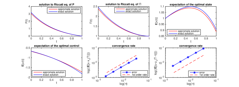
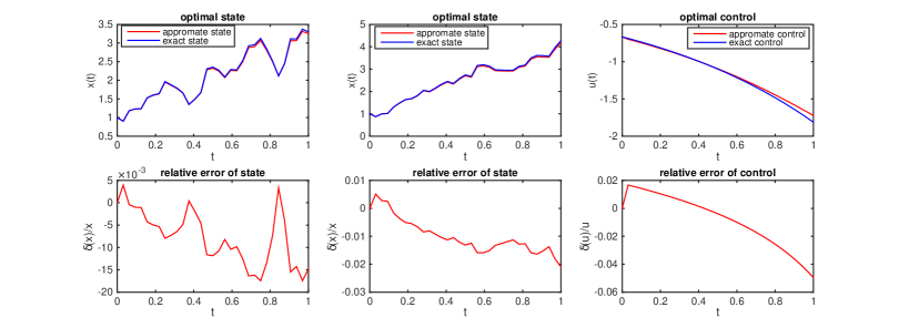
Figure 1: Numerical results for Example 3.12. $\delta(x)/x:=\frac{x_{\tau}(\cdot)-x^{*}(\cdot)}{x^{*}(\cdot)}$ and $\delta(u)/u:=\frac{u_{\tau}(\cdot)-u^{*}(\cdot)}{u^{*}(\cdot)}$.

In the first two figures of Figure 1, we plot the exact solutions to Riccati equations (2.3) and (2.4), the numerical solutions by Algorithm 1 respectively, with the time step $\displaystyle\tau=2^{-5}$. In the third and fourth figures, we plot the expectation of the optimal pair, and its numerical counterpart by Algorithm 1, with the time step $\displaystyle\tau=2^{-5}$. In the fifth and sixth figures, to demonstrate the convergence rate, we plot the corresponding convergence curves. For reference, we add dashed red lines of slope $1$. In the seventh and eighth figures, we plot two path of the optimal state, and in tenth and eleventh figures, we show the relative error of the optimal state, with the time step $\displaystyle\tau=2^{-5}$. The remaining two figures show the error and the relative error of the optimal control, with the time step $\displaystyle\tau=2^{-5}$.

References

[1]N. U. Ahmed, Nonlinear diffusion governed by McKean-Vlasov
equation on Hilbert space and optimal control, SIAM J. Control Optim., 46
(2007), pp. 356–378.
[2]M. Ait Rami, X. Chen, and X. Y. Zhou, Discrete-time indefinite LQ
control with state and control dependent noises, J. Global Optim., 23
(2002), pp. 245–265.
[3]D. Andersson and B. Djehiche, A maximum principle for SDEs of
mean-field type, Appl. Math. Optim., 63 (2011), pp. 341–356.
[4]R. Archibald, F. Bao, and J. Yong, A stochastic gradient descent
approach for stochastic optimal control, East Asian J. Appl. Math., 10
(2020), pp. 635–658.
[5]R. Archibald, F. Bao, J. Yong, and T. Zhou, An efficient numerical
algorithm for solving data driven feedback control problems, J. Sci.
Comput., 85 (2020), pp. Paper No. 51, 27.
[6]C. Beck, W. E, and A. Jentzen, Machine learning approximation
algorithms for high-dimensional fully nonlinear partial differential
equations and second-order backward stochastic differential equations, J.
Nonlinear Sci., 29 (2019), pp. 1563–1619.
[7]R. Bellman, Dynamic programming, Princeton University Press,
Princeton, N. J., 1957.
[8]C. Bender and R. Denk, A forward scheme for backward SDEs,
Stochastic Process. Appl., 117 (2007), pp. 1793–1812.
[9]V. G. Boltyanskii, R. V. Gamkrelidze, and L. S. Pontryagin, On
the theory of optimal processes, Dokl. Akad. Nauk SSSR (N.S.), 110 (1956),
pp. 7–10.
[10]P. Briand and C. Labart, Simulation of BSDEs by Wiener chaos
expansion, Ann. Appl. Probab., 24 (2014), pp. 1129–1171.
[11]R. Buckdahn, B. Djehiche, and J. Li, A general stochastic maximum
principle for SDEs of mean-field type, Appl. Math. Optim., 64 (2011),
pp. 197–216.
[12]M. G. Crandall, H. Ishii, and P.-L. Lions, User’s guide to viscosity
solutions of second order partial differential equations, Bull. Amer. Math.
Soc. (N.S.), 27 (1992), pp. 1–67.
[13]N. Du, J. Shi, and W. Liu, An effective gradient projection method
for stochastic optimal control, Int. J. Numer. Anal. Model., 10 (2013),
pp. 757–774.
[14]T. Dunst and A. Prohl, The forward-backward stochastic heat
equation: numerical analysis and simulation, SIAM J. Sci. Comput., 38
(2016), pp. A2725–A2755.
[15]R. Elliott, X. Li, and Y.-H. Ni, Discrete time mean-field stochastic
linear-quadratic optimal control problems, Automatica J. IFAC, 49 (2013),
pp. 3222–3233.
[16]X. Feng, R. Glowinski, and M. Neilan, Recent developments in
numerical methods for fully nonlinear second order partial differential
equations, SIAM Rev., 55 (2013), pp. 205–267.
[17]X. Feng and M. Jensen, Convergent semi-Lagrangian methods for the
Monge-Ampère equation on unstructured grids, SIAM J. Numer. Anal.,
55 (2017), pp. 691–712.
[18]E. Gobet, J.-P. Lemor, and X. Warin, A regression-based Monte
Carlo method to solve backward stochastic differential equations, Ann.
Appl. Probab., 15 (2005), pp. 2172–2202.
[19]B. Gong, W. Liu, T. Tang, W. Zhao, and T. Zhou, An efficient
gradient projection method for stochastic optimal control problems, SIAM J.
Numer. Anal., 55 (2017), pp. 2982–3005.
[20]Y. Hu, D. Nualart, and X. Song, Malliavin calculus for backward
stochastic differential equations and application to numerical solutions,
Ann. Appl. Probab., 21 (2011), pp. 2379–2423.
[21]J. Huang, X. Li, and J. Yong, A linear-quadratic optimal control
problem for mean-field stochastic differential equations in infinite
horizon, Math. Control Relat. Fields, 5 (2015), pp. 97–139.
[22]R. E. Kalman, Contributions to the theory of optimal control, Bol.
Soc. Mat. Mexicana (2), 5 (1960), pp. 102–119.
[23]H. J. Kushner, On the stochastic maximum principle: Fixed time of
control, J. Math. Anal. Appl., 11 (1965), pp. 78–92.
[24]X. Li, J. Sun, and J. Xiong, Linear quadratic optimal control
problems for mean-field backward stochastic differential equations, Appl.
Math. Optim., 80 (2019), pp. 223–250.
[25]T. Meyer-Brandis, B. Oksendal, and X. Y. Zhou, A mean-field
stochastic maximum principle via Malliavin calculus, Stochastics, 84
(2012), pp. 643–666.
[26]S. Peng, A general stochastic maximum principle for optimal control
problems, SIAM J. Control Optim., 28 (1990), pp. 966–979.
[27]H. Pham, Linear quadratic optimal control of conditional
McKean-Vlasov equation with random coefficients and applications,
Probab. Uncertain. Quant. Risk, 1 (2016), pp. Paper No. 7, 26.
[28]A. Prohl and Y. Wang, Strong rates of
convergence for a space-time discretization of the backward stochastic heat
equation, and of a linear-quadratic control problem for the stochastic heat
equation, ESAIM Control Optim. Calc. Var., 27 (2021), pp. Paper No. 54, 30.
[29]A. Prohl and Y. Wang, Strong error
estimates for a space-time discretization of the linear-quadratic control
problem with the stochastic heat equation with linear noise, IMA J. Numer.
Anal., 42 (2022), pp. 3386–3429.
[30]P. Wang and X. Zhang, Numerical solutions of backward stochastic
differential equations: a finite transposition method, C. R. Math. Acad.
Sci. Paris, 349 (2011), pp. 901–903.
[31]Y. Wang, Error analysis of a discretization for stochastic linear
quadratic control problems governed by SDEs, IMA J. Math. Control Inform.,
38 (2021), pp. 1148–1173.
[32]Y. Wang, Error analysis of
the feedback controls arising in the stochastic linear quadratic control
problems, J. Syst. Sci. Complex., Accepted, (2022).
[33]J. Yong, Linear-quadratic optimal control problems for mean-field
stochastic differential equations, SIAM J. Control Optim., 51 (2013),
pp. 2809–2838.
[34]J. Yong and X. Y. Zhou, Stochastic controls: Hamiltonian systems and
HJB equations, vol. 43 of Applications of Mathematics (New York),
Springer-Verlag, New York, 1999.
[35]J. Zhang, A numerical scheme for BSDEs, Ann. Appl. Probab., 14
(2004), pp. 459–488.