Domain Adaptation for Time Series Under Feature and Label Shifts

xF

Abstract

Unsupervised domain adaptation (UDA) enables the transfer of models trained on source domains to unlabeled target domains. However, transferring complex time series models presents challenges due to the dynamic temporal structure variations across domains. This leads to feature shifts in the time and frequency representations. Additionally, the label distributions of tasks in the source and target domains can differ significantly, posing difficulties in addressing label shifts and recognizing labels unique to the target domain. Effectively transferring complex time series models remains a formidable problem. We present Raincoat, the first model for both closed-set and universal domain adaptation on complex time series. Raincoat addresses feature and label shifts by considering both temporal and frequency features, aligning them across domains, and correcting for misalignments to facilitate the detection of private labels. Additionally, Raincoat improves transferability by identifying label shifts in target domains. Our experiments with 5 datasets and 13 state-of-the-art UDA methods demonstrate that Raincoat can improve transfer learning performance by up to 16.33% and can handle both closed-set and universal domain adaptation.

Require:Input: Ensure:Output:

1 Introduction

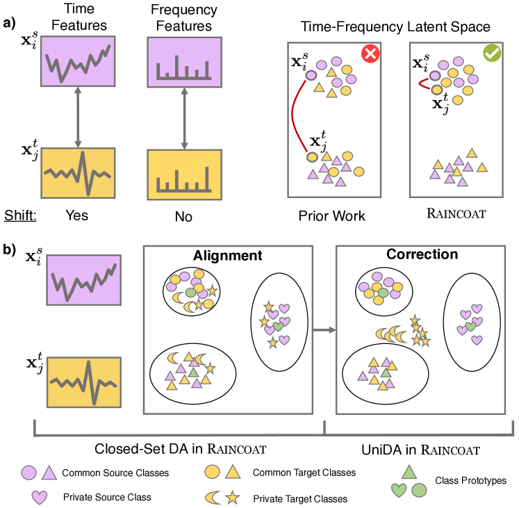
Figure 1: a) Raincoat captures domain-invariant frequency features under feature and label shifts. b) For Closed-Set DA, Raincoat aligns source and target domains for greater generalization. For Universal DA, the correction step prioritizes target-specific features to detect private target classes.

Neural networks have demonstrated impressive performance on time series datasets (ravuri2021skilful; lundberg2018explainable). However, their performance deteriorates rapidly under domain shifts, making it challenging to deploy these models in real-world scenarios (TF-C; zhang2022graph). Domain shifts occur when the test distribution is not identical to the training data, even though it is often related (wilds2021; Luo2018TakingAC; Zhang2013DomainAU), meaning that latent representations do not generalize to test datasets drawn from different underlying distributions, even if the differences between these distributions are minor. To overcome these challenges, domain adaptation (DA) has emerged as a set of techniques that allow adaptation to new target domains and reduce bias by leveraging unlabeled data in target domains (Ganin:2016; DAN).

Training models that can adapt to domain shifts is crucial for robust, real-world deployment. For instance, for healthcare time series, data collection methods vary widely across different clinical sites (domains) (zhang2022shifting), leading to shifts in the underlying features and labels. It is preferable to train a model on a diverse dataset collected from multiple clinics rather than training and applying individual models on smaller, single-domain datasets for each clinic. Additionally, training a model that can detect unknown classes in test data, such as patients with rare diseases (alsentzer2022deep), is advantageous for real-world implementation among end-users, such as clinicians (tonekaboni2019clinicians). Endowing learning systems with DA capabilities can increase their reliability and expand applicability across downstream tasks.

DA is a highly complex problem due to several factors. First, models trained for robustness to domain shifts must learn highly generalizable features; however, neural networks trained using standard practices can rely on spurious correlations created by non-causal data artifacts (geirhos2020shortcut; degrave2021radiographic), hindering their ability to transfer across domains. Additionally, shifts in label distributions across domains may result in private labels, i.e., classes that exist in the target domain but not in the source domain (Lipton2018DetectingAC). In unsupervised DA, a model must generalize across domains when labels from the target domain are not available during training (long2018conditional; Kang2019ContrastiveAN). Therefore, DA methods must be able to identify when a private label is encountered in the target domain without any prior supervision on detecting these unknown labels (You2019UniversalDA; Fu2020LearningTD). Yet, that is not possible by techniques that rely on training samples that simulate predicting unknown labels. This highlights the need for time series DA methods that 1) produce generalizable representations robust to feature and label shifts, and 2) expand the scope of existing DA methods by supporting both closed-set and universal DA.

DA becomes even more challenging when applied to time series data. Domain shifts can occur in both the time and frequency features of time series, which can create a shift that highly perturbs time features while frequency features are relatively unchanged, or vice versa (Figure 1a). Previous time series DA methods fail to explicitly model frequency features. Further, models can fail to generalize due to shortcut learning (brown2022detecting), which occurs when the model focuses on time-space features while overlooking crucial underlying concepts in the frequency-space domain, leading to limited poor performance on data unseen during training. Additionally, universal DA—when no assumptions are made about the overlap between labels in the source and target domains—is an unexplored area in time series research (Figure 1b).

Present Work. We introduce Raincoat (fRequency-augmented AlIgN-then-Correct for dOmain Adaptation for Time series), a novel domain adaptation method for time series data that can handle both feature and label shifts (as shown in Figure 1). Our method is the first to address both closed-set and universal domain adaptation for time series and has the unique capability of handling feature and label shifts. To achieve this, we first use time and frequency-based encoders to learn time series representations, motivated by inductive bias that domain shifts can occur via both time or frequency feature shifts. We use Sinkhorn divergence for source-target feature alignment and provide both empirical evidence and theoretical justification for its superiority over other popular divergence measures. Finally, we introduce an “align-then-correct” procedure for universal DA, which first aligns the source and target domains, retrains the encoder on the target domain to correct misalignments, and then measures the difference between the aligned and corrected representations of target samples to detect unknown target classes (as shown in Figure 2). We evaluate Raincoat on five time-series datasets from various modalities, including human activity recognition, mechanical fault detection, and electroencephalogram prediction. Our method outperforms strong baselines by up to 9.0% for closed-set DA and 16.33% for universal DA. Raincoat is available at https://github.com/mims-harvard/Raincoat.

2 Related Work

General Domain Adaptation. General domain adaptation (DA), leveraging labeled source domain to predict labels on the unlabeled target domain, has a wide range of applications (ganin2015unsupervised; sener2016learning; zhang2018task; perone2019unsupervised; ramponi2020neural). We organize DA methods into three categories: 1) Adversarial training: A domain discriminator is optimized to distinguish source and target domains, while a deep classification model learns transferable features indistinguishable by the domain discriminator (Hoffman2015SimultaneousDT; tzeng2017adversarial; motiian2017few; long2018conditional; hoffman2018cycada). 2) Statistical divergence: These approaches aim to extract domain invariant features by minimizing domain discrepancy in a latent feature space. Widely used measures include MMD (Rozantsev2016BeyondSW), correlation alignment (CORAL) (dcoral), contrastive domain discrepancy (CDD) (Kang2019ContrastiveAN), optimal transport distance (courty2017joint; redko2019optimal), and graph matching loss (Yan2016ASS; Das2018UnsupervisedDA). 3) Self-supervision: These general DA approaches incorporate auxiliary self-supervision training tasks. These methods learn domain-invariant features through a pretext learning task, such as data augmentation and reconstruction, for which a target objective can be computed without supervision (kang2019contrastive; singh2021clda; tang2021gradient). In addition, reconstruction-based methods achieve alignment by carrying out source domain classification and reconstruction of target domain data or both source and target domain data (ghifary2016deep; jhuo2012robust). Raincoat sits in the category of both 2 and 3.

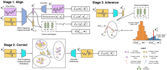
Figure 2: Illustration of the Raincoat method for time series DA. Details provided in-text.

Domain Adaptation for Time Series. While in light of successes in computer vision, limited methods have focused on adaptation approaches for time series data. To date, few DA methods are specifically designed for time series. 1) Adversarial training: VRADA (Purushotham2017VariationalRA) builds upon a variational recurrent neural network (VRNN) and trains adversarially to capture complex temporal relationships that are domain-invariant. CoDATS (Wilson2020MultiSourceDD) builds upon VRADA but uses a convolutional neural network for the feature extractor. 2) Statistical divergence: SASA (Cai2021TimeSD) aligns the condition distribution of the time series data by minimizing the discrepancy of the associative structure of time series variables between domains. AdvSKM (ijcai2021p378) and (Ott2022DomainAF) are metric-based methods that align two domains by considering statistic divergence. 3) Self-supervision: DAF (DAF-icml) extracts domain-invariant and domain-specific features to perform forecasts for source and target domains through a shared attention module with a reconstruction task. CLUDA (Ozyurt2022ContrastiveLF) and CLADA (CALDA) are two contrastive DA methods that use augmentations to extract domain invariant and contextual features for prediction. However, the above methods align features without considering the potential gap between labels from both domains. Moreover, they focus on aligning only time features while ignoring the implicit frequency feature shift (Fig. 1a). In contrast, Raincoat considers the frequency feature shift to mitigate both feature and label shift in DA.

Universal Domain Adaptation. Prevailing DA methods assume all labels in the target domain are also available in the source domain. This assumption, known as closed-set DA, posits that the domain gap is driven by feature shift (as opposed to label shift). However, the label overlap between the two domains is unknown in practice. Thus, assuming both feature and label shifts can cause the domain gap is more practical. In contrast to closed-set DA, universal domain adaptation (UniDA) (You2019UniversalDA) can account for label shift. UniDA categorizes target samples into common labels (present in both source and target domains) or private labels (present in the target domain only). UAN (You2019UniversalDA), CMU (Fu2020LearningTD), and TNT (Chen2022EvidentialNC) use sample-level uncertainty criteria to measure domain transferability. Samples with lower uncertainty are preferentially selected for adversarial adaptation. However, most UniDA methods detect common samples using sample-level criteria, requiring users to specify the threshold to recognize private labels. Moreover, over-reliance on source supervision neglects discriminative representation in the target domain. DANCE (Saito2020UniversalDA) uses self-supervised neighborhood clustering to learn features to discriminate private labels. Similarly, DCC (Li2021DomainCC) enumerates cluster numbers of the target domain to obtain optimal cross-domain consensus clusters as common classes. Still, the consensus clusters are not robust enough due to challenging cluster assignments. MATHS (Chen2022MutualNN) detects private labels via mutual nearest-neighbor contrastive learning. In contrast, UniOT (Chang2022UnifiedOT) uses optimal transport to detect common samples and produce representations for samples in the target domain. However, these methods use a feature encoder shared across both domains even though the source and target domains are shifted. In addition, most require fine-tuned thresholds to recognize private labels.

3 Problem Setup and Formulation

Notation. We are given a dataset $\mathcal{D}=\{(\mathbf{x}_{i},y_{i})\}_{i=1}^{n}$ of $n$ multivariate time series samples where $i$-th sample $\mathbf{x}_{i}\in\mathbb{R}^{T\times d}$ contains readouts of $d$ sensors over $T$ time points. Without loss of generality, we consider regular time series — Raincoat can be used with techniques, such as Raindrop (zhang2022graph) to handle irregular time series. We use $\mathbf{x}_{i}$ to denote a time series (both univariate and multivariate). Each label $y_{i}$ in $\mathcal{D}$ belongs to the label set $\mathcal{C}$, i.e., $y_{i}\in\mathcal{C}$. We use $\mathcal{D}^{s}=\left\{\left(\mathbf{x}_{i}^{s},y_{i}^{s}\right)\right\}_{i=1}^{n_{s}}$ to denote the source domain dataset with $n_{s}$ labeled samples, where $\mathbf{x}_{i}^{s}$ is a source domain sample and $y^{s}_{i}$ is the associated label. The target domain dataset is unlabeled and denoted as $\mathcal{D}^{t}=\left\{\left(\mathbf{x}_{i}^{t}\right)\right\}_{i=1}^{n_{t}}$ with $n_{t}$ unlabeled samples. Source and target label sets are denoted as $\mathcal{C}^{s}$ and $\mathcal{C}^{t}$, respectively. Zero, one or more labels may be shared between source and target domains, which we denote as $\mathcal{C}^{s,t}=\mathcal{C}^{s}\cap\mathcal{C}^{t}$. Source and target domains have samples drawn from source and target distributions, $\mathcal{D}^{s}\sim p_{s}(\mathbf{x}^{s},y^{s})$ and $\mathcal{D}^{t}\sim p_{t}(\mathbf{x}^{t},y^{t})$.

We consider two types of domain shifts: feature shift and label shift. Feature shift occurs when marginal probability distributions of $\mathbf{x}$ differ, $p_{s}(\mathbf{x})\neq p_{t}(\mathbf{x})$, while conditional probability distributions remain constant across domains, $p_{s}(y|\mathbf{x})=p_{t}(y|\mathbf{x})$ (Zhang2013DomainAU). Label shift occurs when marginal probability distributions of $y$ differ, $p_{s}(y)\neq p_{t}(y)$. Feature shifts may occur in time series due to, for example, differences in sensor measurement setup or length of samples. A unique property of time series is that feature shifts may occur in both time and frequency spectra. The importance of modeling shifts in both the time and frequency spectrum is discussed in later sections. Label shift may occur as either a change in the proportion of classes in either domain or as a categorical shift: both domains might contain different classes in their label sets.

Problem 3.1 (Closed-set Domain Adaptation for Time Series Classification).

Given the source and target domain time series datasets, $\mathcal{D}^{s}$ and $\mathcal{D}^{t}$, whose label sets are the same, $\mathcal{C}^{s}=\mathcal{C}^{t}$, and target labels $y^{t}$ are not available at train time. Raincoat specifies a strategy to train a classifier $f$ on $\mathcal{D}^{s}$ such that $f$ generalizes to $\mathcal{D}^{t}$, i.e., it minimizes classification risk on $\mathcal{D}^{t}$: $\mathbb{E}_{\mathbf{x}_{i},y_{i}\sim\mathcal{D}^{t}}\left[\mathcal{L}_{C}(f(\mathbf{x}_{i}),y_{i})\right]$, where $\mathcal{L}_{C}$ is a classification loss function.

In a real-world application, little information may be available on the feature or label distribution of the target domain. Private labels in either the source or target domain may exist, i.e., classes present in one domain but absent in the other. Thus, it is desirable to relax the strict assumption of $\mathcal{C}^{s}=\mathcal{C}^{t}$ made by Problem 3.1. We denote source private labels as $\bar{\mathcal{C}}^{s}=\mathcal{C}^{s}\setminus\mathcal{C}^{t}$, target private labels as $\bar{\mathcal{C}}^{t}=\mathcal{C}^{t}\setminus\mathcal{C}^{s}$, and labels shared between domains as $\mathcal{C}^{s,t}=\mathcal{C}^{s}\cap\mathcal{C}^{t}$. We denote the access of samples in dataset $\mathcal{D}$ belonging to label set $\mathcal{C}$ as $\mathcal{D}[\mathcal{C}]$, e.g., samples in the target domain belonging to the common label set would be denoted as $\mathcal{D}^{t}[\mathcal{C}^{s,t}]$. Domains might not have common labels, $\mathcal{C}^{s,t}=\emptyset$, leading to the definition of universal DA.

Problem 3.2 (Universal Domain Adaptation (UniDA) for Time Series Classification).

Given our source and target domain time series datasets, $\mathcal{D}^{s}$ and $\mathcal{D}^{t}$, where target labels $y^{t}$ are unavailable at train time. Raincoat specifies a stratefy to train a classifier $f$ on $\mathcal{D}^{s}$ such that $f$ generalizes to $\mathcal{D}^{t}$, i.e., it minimizes classification risk of a loss function $\mathcal{L}_{C}$ on samples belonging to $\mathcal{C}^{s,t}$ in $\mathcal{D}^{t}$: $\mathbb{E}_{\mathbf{x}_{i},y_{i}\sim\mathcal{D}^{t}[\mathcal{C}^{s,t}]}\left[\mathcal{L}_{C}(f(\mathbf{x}_{i}),y_{i})\right]$, while identifying samples in private target classes, $\mathbf{x}_{i}\sim\mathcal{D}^{t}[\bar{\mathcal{C}}^{t}]$, as unknown samples.

4 Preliminaries

Discrete Fourier Transform. Given a series sample $\mathbf{x}$ with $d$ channels and $T$ time points, it is transformed to the frequency space by applying the 1-dim DFT of length $T$ to each channel and then transforming it back using the 1-dim inverse DFT, defined as:

$$\text{Forward DFT}: \quad\mathbf{v}[m]=\textstyle\sum_{t=0}^{T-1}\mathbf{x}[t]\cdot e^{-i2\pi\frac{mt}{T}}$$ (1)

$$\text{Inverse DFT}: \quad\mathbf{x}[n]=\frac{1}{T}\textstyle\sum_{t=0}^{T-1}\mathbf{v}[m]\cdot e^{i\cdot 2\pi\frac{mt}{T}}$$

where $T=$ number of points, $n$ = current point index, $m$ = current frequency index, where $m\in[0,T-1]$. We denote the extracted amplitude and phase as $\mathbf{a}$ and $\mathbf{p}$ respectively:

$$\mathbf{a}[m] =\frac{\left|\mathbf{v}[m]\right|}{T}=\frac{\sqrt{\operatorname{Re}\left(\mathbf{v}[m]\right)^{2}+\operatorname{Im}\left(\mathbf{v}[m]\right)^{2}}}{T}$$ (2)

$$\mathbf{p}[m] =\operatorname{atan2}\left(\operatorname{Im}\left(\mathbf{v}[m]\right),\operatorname{Re}\left(\mathbf{v}[m]\right)\right)$$

where Im$(\mathbf{v}[m])$ and Re$(\mathbf{v}[m])$ indicate imaginary and real parts of a complex number, and atan2 is the two-argument form of arctan.

5 Raincoat Approach

We start with an overview of Raincoat and proceed with (5.2) time-frequency encoding, (5.3) feature alignment, (5.4) unknown sample detection, and (5.5) training and inference.

5.1 Overview

Raincoat is an unsupervised method for closed set and universal domain adaptation in time series, addressing Problems 3.1-3.2. Raincoat consists of three modules: a time-frequency encoder $G_{\textsc{T}\textsc{F}}$, a classifier $H$, and an auxiliary decoder $U_{\textsc{T}\textsc{F}}$. Sec. 5.2 describes the encoder $G_{\textsc{T}\textsc{F}}$, which leverages both time and frequency features. Sec. 5.3 describes how Sinkhorn divergence is a suitable divergence measurement to align the source and target domain because frequency features may not share the same support across both domains. Sec. 5.4 motivates the correction step for UniDA. Sec. 5.5 describes how Raincoat detects potential unknown samples through analysis of pre- and post-correction embeddings. Finally, Sec. LABEL:sec:training provides an overview of Raincoat models.

5.2 Time-Frequency Feature Encoder

We begin by highlighting the significance of frequency features in DA for time series. Although various methods have been proposed to solve the time series DA problem under the assumption of feature shift, none of them explicitly address situations where changes in the frequency domain also act as an implicit feature shift. To fill this gap, Raincoat encodes both time and frequency features in its latent representations. The source frequency and time features are denoted as $\mathbf{e}_{\textsc{F},i}^{s}$ and $\mathbf{e}_{\textsc{T},i}^{s}$, respectively, while the target frequency and time features are represented as $\mathbf{e}_{\textsc{F},i}^{t}$ and $\mathbf{e}_{\textsc{T},i}^{t}$. For simplicity, the superscript indicating the source or target domain is omitted in the rest of the text.

Shift of Frequency Features. We formalize the frequency shift of time series as another type of feature shift. For this purpose, we use the Fourier transform, with the possibility of exploring other options such as wavelets left for future work. A time series $\mathbf{x}_{i}$ can be represented as a combination of sinusoids, each with a specific frequency, amplitude, and phase, as explained in Sec. 4. If the conditional distributions of the labels with respect to the frequency features are equal ($p_{s}(y|DFT(\mathbf{x}^{s}))=p_{t}(y|DFT(\mathbf{x}^{t}))$), but the domains have different frequency features ($p(DFT(\mathbf{x}^{s}))\neq p(DFT(\mathbf{x}^{t}))$), then a frequency shift occurs.

Frequency Features Promote Domain Adaptation. BenDavid2006AnalysisOR; BenDavid2010ATO demonstrated that the performance of DA techniques is bounded by the divergence between the source and target domains, and that a small feature shift is necessary for DA techniques to be effective. However, unsupervised DA methods for time series align only time features ($\mathbf{e}_{\textsc{T},i}^{s}$ and $\mathbf{e}_{\textsc{T},i}^{t}$), leading to sub-optimal performance when the time feature shift is large. By including frequency features in the encoder $G_{\textsc{T}\textsc{F}}$, we can uncover potential invariant features across domains and improve transferability. For instance, Figure 3 illustrates the sensor readings of walking activity from two different individuals ($\mathbf{x}_{i}^{s}$ and $\mathbf{x}_{i}^{t}$) in the WISDM dataset (10.1145/1964897.1964918) and their corresponding Fourier features ($\mathbf{e}_{\textsc{F},i}^{s}$ and $\mathbf{e}_{\textsc{F},i}^{t}$). Using only time features would result in poor predictions in the target domain due to a significant time feature shift between $\mathbf{x}_{i}^{s}$ and $\mathbf{x}_{i}^{t}$. On the other hand, frequency features from different domains do not exhibit significant feature shifts and thus are domain invariant. This suggests that incorporating frequency features can lead to more accurate predictions in the target domain as DA aims to extract domain-invariant features. For this reason, Raincoat uses both time and frequency features in domain alignment.

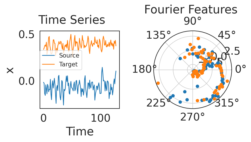
Figure 3: Left: averaged sensor readings (one channel) of the walking activity collected from two persons (source and target). Right: corresponding polar coordinates of Fourier features. Fourier features are more domain-invariant than time features.

Frequency Feature Encoder. Inspired by Fourier neural operator (FNO) (li2021fourier), Raincoat applies convolution on low-frequency modes of the Fourier transform of $\mathbf{x}_{i}$. We make two modifications to improve the utility of Fourier convolution for DA: 1) Prevent Frequency Leakage: Discrete Fourier Transform considers inputs $\mathbf{x}_{i}$ to be periodic. Violation of such assumption results in frequency leakage (Harris1978OnTU). Specifically, given two window sliced time series $\mathbf{x}_{i}^{s}$ and $\mathbf{x}_{i}^{t}$ , applying DFT  (1) could return perturbed and noisy $\mathbf{v}_{i}^{s}$ and $\mathbf{v}_{i}^{t}$ which may lead to noisy-biased domain alignment. To prevent aligning on noisy frequency features, Raincoat applies a smoothing function (cosine function) before applying DFT. 2) Consider amplitude $\mathbf{a}_{i}$ and phase $\mathbf{p}_{i}$ information: Instead of using inverse DFT to convert $\mathbf{v}_{i}$ back to time-space which is an unnecessary step for frequency feature extraction, Raincoat extracts the polar coordinates of frequency coefficients to keep both low-level ($\mathbf{a}_{i}$) and high-level ($\mathbf{p}_{i}$) semantics. The frequency space features $\mathbf{e}_{\textsc{F}}$ is a concatenation $[\mathbf{a}_{i};\mathbf{p}_{i}]$.

Now we summarize how $G_{\textsc{F}\textsc{T}}$ encodes time-frequency feature from $\mathbf{x}_{i}$. Define a convolution operator “$\ast$” and weight matrix $\mathbf{B}$, the encoder $G_{\textsc{F}}$ encodes frequency features $\mathbf{e}_{\textsc{F},i}$ by: 1) Smooth: $\mathbf{x}_{i}=\operatorname{Smooth}(\mathbf{x}_{i})$, 2) DFT: $\mathbf{v}_{i}=\operatorname{DFT}(\mathbf{x}_{i})$, 3) Convolution: $\tilde{\mathbf{v}}_{i}=\mathbf{B}\ast\mathbf{v}_{i}$, 4) Transform: $\mathbf{a}_{i},\mathbf{p}_{i}\leftarrow\tilde{\mathbf{v}}_{i}\text{ (Use Eq.~{}\ref{eqn:ap})}$, 5) Extract: $\mathbf{e}_{\textsc{F},i}=[\mathbf{a}_{i};\mathbf{p}_{i}]$ The time features $\mathbf{e}_{\textsc{T},i}$ can be obtained using any existing time feature encoder, such as CNNs. Finally, the latent representation $\mathbf{z}_{i}$ is a concatenation of frequency and time features $[\mathbf{e}_{\textsc{F},i};\mathbf{e}_{\textsc{T},i}]$. Details are in Appendix LABEL:asec:encoder.

5.3 Domain Alignment of Time-Frequency Features

Next, we address the question of what is the appropriate metric to align frequency features between $\mathbf{e}_{\textsc{F}}^{s}$ and $\mathbf{e}_{\textsc{F}}^{t}$. Raincoat represents the frequency features as the amplitude and phase, $\mathbf{e}_{\textsc{F},i}^{s}=[\mathbf{a}^{s}_{i};\mathbf{p}^{t}_{i}],\mathbf{e}_{\textsc{F},i}^{t}=[\mathbf{a}^{t}_{i};\mathbf{p}^{t}_{i}]$, meaning that the frequency feature shift can be represented as $p_{s}(\mathbf{a}^{s},\mathbf{p}^{s})\neq p_{t}(\mathbf{a}^{t},\mathbf{p}^{t})$.

Disjoint Support Sets for Frequency Features. An appropriate metric to align frequency features between $\mathbf{e}_{\textsc{F}}^{s}$ and $\mathbf{e}_{\textsc{F}}^{t}$ is challenging to find. Distance measures such as the total variation distance or Kullback-Leibler divergence are not suitable because they are unstable when the supports of distributions are deformed and do not metricize the convergence in law (Feydy:2019), meaning that they do not effectively capture the discrepancy when $\mathbf{e}^{s}_{\textsc{F},i}$ and $\mathbf{e}^{t}_{\textsc{F},i}$ have disjoint support. The KL divergence, for example, grows unbounded ($KL(\mathbf{e}_{\textsc{F},i}^{s}||\mathbf{e}_{\textsc{F},i}^{t})\to+\infty$) when $\mathbf{e}_{\textsc{F},i}^{t}$ and $\mathbf{e}_{\textsc{F},i}^{t}$ are far apart, leading to a degradation of alignment and early collapse. An ideal divergence measure could capture the discrepancy even if $\mathbf{e}^{s}_{\textsc{F},i}$ and $\mathbf{e}^{t}_{\textsc{F},i}$ have disjoint support ($\textrm{supp}(\mathbf{e}^{s}_{\textsc{F},i})\cap\textrm{supp}(\mathbf{e}^{t}_{\textsc{F},i})\approx\emptyset$).

The components of frequency features, amplitude $\mathbf{a}$ and phase $\mathbf{p}$, have different distributions. The phase $\mathbf{p}$ has a uniform distribution over the range of polar angles, which makes it easy to measure the distance between $\mathbf{p}^{s}_{i}$ and $\mathbf{p}^{t}_{i}$, bounded in the polar coordinate system $\mathbf{p}_{i}\in[0,2\pi)$. However, the amplitude $\mathbf{a}$ has a Rayleigh distribution with an unlimited scale, $\mathbf{a}_{i}\in[0,+\infty)$, making it difficult to measure the distance between $\mathbf{a}^{s}_{i}$ and $\mathbf{a}^{t}_{i}$ using the KL divergence. The KL divergence can not provide useful gradients when $\mathbf{a}_{i}^{s}$ are $\mathbf{a}_{i}^{t}$ are far apart. This leads to a lack of alignment when the amplitudes are far apart, as numerically verified in Figure LABEL:fig:sinkhorn_motivation in the Appendix.

Sinkhorn Divergence. The Sinkhorn divergence is an entropy-regularized optimal transport distance that enables the comparison of distributions with disjoint supports. Another metric, maximum mean discrepancy (MMD), addresses the issue of disjoint support by considering the geometry of the distributions. However, we demonstrate that MMD has a theoretical weakness that manifests as vanishing gradients or similar artifacts. To address this, Raincoat aligns the source features ($\mathbf{z}^{s}_{i}$) and target features ($\mathbf{z}^{t}_{i}$) by minimizing a domain alignment loss based on Sinkhorn. Further details are provided in Appendix LABEL:sec:appendixMMD.

5.4 Correction Step in Raincoat

In this section, we explain how the correction step helps reduce negative transfer by rejecting target unknown samples $\mathbf{x}^{t}\sim\mathcal{D}^{t}[\bar{\mathcal{C}}^{t}]$. The correction step updates the encoder $G_{\textsc{T}\textsc{F}}$ and decoder $U_{\textsc{T}\textsc{F}}$ by solving a reconstruction task on target samples $\mathbf{x}^{t}\sim\mathcal{D}^{t}$. This updated $G_{\textsc{T}\textsc{F}}$ repositions the target features $\mathbf{z}^{t}_{i}$. The target features before and after the correction step are denoted as $\mathbf{z}^{t}_{a,i}$ and $\mathbf{z}^{t}_{c,i}$, respectively.

Motivation for Reconstructing $\mathbf{x}^{t}_{i}$. The cluster assumption (Chapelle2005SemiSupervisedCB) holds that the input data is separated into clusters and that samples within the same cluster have the same label. Based on this, we argue that preserving target discriminative features $\mathbf{z}^{t}_{i}$ is important for UniDA, because such features help generate discriminative clusters, including clusters of target unknown samples, which improves UniDA. To do this, Raincoat minimizes a reconstruction loss to adapt the feature encoder $G_{\textsc{T}\textsc{F}}$ and decoder $U_{\textsc{T}\textsc{F}}$. The target features $\mathbf{z}_{a,i}^{t}$ before the correction step are generated by a shared encoder $G_{\textsc{T}\textsc{F}}$ that aligns the source and target domains. As a result, the target features of common samples $\mathbf{x}^{t}\sim\mathcal{D}^{t}[\mathcal{C}^{s,t}]$ should change less in the latent space than those of target unknown samples $\mathbf{x}^{t}\sim\mathcal{D}^{t}[\bar{\mathcal{C}}^{t}]$. This indicates that the corrected encoder $G_{\textsc{T}\textsc{F}}$ maintains the features of common target samples close to their originally assigned label while letting the features of target unknown samples diverge from their originally assigned label. Raincoat leverages this to detect and reject target unknown samples, which we discuss next.

5.5 Inference: Detect Target Private Samples

Raincoat detects target unknown samples $\mathbf{x}^{t}\sim\mathcal{D}^{t}[\bar{\mathcal{C}}^{t}]$ by determining the movement of target features before and after the correction step. It assumes that when the target domain contains unknown labels, the distribution of the movement will exhibit a bimodal structure.

For brevity, the feature vector $\mathbf{z}^{t}_{i}$ is used as an input to $H$, which consists of prototypes for each class $\mathbf{W}=[\mathbf{w}_{1},\mathbf{w}_{2},\cdots,\mathbf{w}_{C}]$. Denote the distance (cosine similarity) of $\mathbf{z}^{t}_{i}$ to its assigned prototype $c$ as $d(\mathbf{z}^{t}_{i},\mathbf{w}_{c})$. Cosine similarity is a reasonable choice because the cross entropy (CE) loss encourages angular separation. It can be interpreted as aligning the feature vectors $\mathbf{z}^{t}_{i}$ along its assigned class prototype. The cosine similarity in the form of the dot product gives CE an intrinsic angular property, which is observed in Eq. 5.5 where features naturally separate in the polar coordinates with CE only. Given a target feature $\mathbf{z}^{t}_{i}$ and true label $y_{i}=c$, the cross entropy can be expressed as:

$$\begin{array}[]{l}\!\!\!\mathcal{L}_{\mathrm{CE}}(\hat{y},y)=-\log\frac{\exp\left(\mathbf{w}_{c}^{T}\mathbf{z}^{t}_{i}\right)}{\sum_{j}\exp\left(\mathbf{w}_{j}^{T}\mathbf{z}^{t}_{i}\right)}\propto\sum\limits_{j\neq c}\exp\left(\mathbf{w}_{j}^{T}\mathbf{z}^{t}_{i}-\mathbf{w}_{c}^{T}\mathbf{z}^{t}_{i}\right)\\ \\ \propto\sum\limits_{j\neq c}\exp\left(\|\mathbf{z}^{t}_{i}\|_{2}\left\|\mathbf{w}_{j}\right\|_{2}\cos\left(\theta_{j}\right)-\|\mathbf{z}^{t}_{i}\|_{2}\left\|\mathbf{w}_{c}\right\|_{2}\cos\left(\theta_{c}\right)\right)\\ \end{array}$$

As a result, if the target feature $\mathbf{z}^{t}_{i}$ is close to its prototypes, then $d(\mathbf{z}^{t}_{i},\mathbf{w}_{c})$ will be small, and vice versa. Then Raincoat measures the movement by calculating the absolute difference of target features’ distance to the assigned prototype before and after correction given by $d^{ac}_{i}=|d(\mathbf{z}^{t}_{a,i},\mathbf{w}_{c})-d(\mathbf{z}^{t}_{c,i},\mathbf{w}_{c})|$.

Next, Raincoat detects if there are private target samples in each class by first running a bimodal test on each group of $\mathcal{C}^{s}$. If the bimodal test tells us $d^{ac}$ has two modes, it then trains a $2$-mean cluster to fit the distribution of $d^{ac}$. For each class, after we obtain the centroid $\mu_{1},\mu_{2}$, where $\mu_{1}<\mu_{2}$, Raincoat takes $\mu_{2}$ as our threshold to reject unknown target samples.

Algorithm 1 Overview of Raincoat

Input: dataset $\mathcal{D}^{s}$, $\mathcal{D}^{t}$; epochs $E_{1},E_{2}$; time-frequency feature encoder, $G_{\textsc{T}\textsc{F}}$, and decoder, $U_{\textsc{T}\textsc{F}}$(Alg. LABEL:alg:freq-align); prototype classifier $H$Stage 1: Alignment(introduced in 5.2, )) $E_{1}$epochs Extract $\mathbf{z}^{s}_{i},\mathbf{z}^{t}_{i}\leftarrow G_{\textsc{T}\textsc{F}}(\mathbf{x}^{s}_{i}),G_{\textsc{T}\textsc{F}}(\mathbf{x}^{t}_{i})$$\mathcal{L}_{A}\leftarrow\textsc{Sinkhorn}(\mathbf{z}^{s}_{i},\mathbf{z}^{t}_{i})$(Alg. ) $\mathcal{L}_{R}\leftarrow|\mathbf{x}^{s}_{i}-U_{\textsc{T}\textsc{F}}(\mathbf{z}^{s}_{i})|$$\mathcal{L}_{C}\leftarrow CE(y^{s}_{i},H(\mathbf{z}^{s}_{i}))$Update $U_{\textsc{T}\textsc{F}},G_{\textsc{T}\textsc{F}},H$with $\nabla(\mathcal{L}_{A}+\mathcal{L}_{R}+\mathcal{L}_{C})$Stage 2: Correction(introduced in ) Extract features: $\mathbf{z}^{t}_{a,i}\leftarrow G_{\textsc{T}\textsc{F}}(\mathbf{x}^{t}_{i})$Distance to prototypes: $\mathbf{d}_{\text{align}}\leftarrow d(\mathbf{z}^{t}_{a,i},H)$$E_{2}$epochs $\mathcal{L}_{R}\leftarrow|\mathbf{x}^{t}_{i}-(U_{\textsc{T}\textsc{F}}\circ G_{\textsc{T}\textsc{F}})(\mathbf{x}^{t}_{i})|$Update $U_{\textsc{T}\textsc{F}},G_{\textsc{T}\textsc{F}}$with $\nabla\mathcal{L}_{R}$Extract post-correction: $\mathbf{z}^{t}_{c,i}\leftarrow G_{\textsc{T}\textsc{F}}(\mathbf{x}^{t}_{I})$Re-compute: $\mathbf{d}_{\text{correct}}\leftarrow d(\mathbf{z}^{t}_{c,i},H)$Stage 3: Inference(introduced in ) $d^{ac}_{i}=|d(\mathbf{z}^{t}_{a,i},\mathbf{w}_{c})-d(\mathbf{z}^{t}_{c,i},\mathbf{w}_{c})|$$c$in $C^{s}$$p\leftarrow\text{Bimodal Test}$$p<0.05$