Asymptotic Representations for Sequential Decisions, Adaptive Experiments, and Batched Bandits

Abstract

We develop asymptotic approximation results that can be applied to sequential estimation and inference problems, adaptive randomized controlled trials, and other statistical decision problems that involve multiple decision nodes with structured and possibly endogenous information sets. Our results extend the classic asymptotic representation theorem used extensively in efficiency bound theory and local power analysis. In adaptive settings where the decision at one stage can affect the observation of variables in later stages, we show that a limiting data environment characterizes all limit distributions attainable through a joint choice of an adaptive design rule and statistics applied to the adaptively generated data, under local alternatives. We illustrate how the theory can be applied to study the choice of adaptive rules and end-of-sample statistical inference in batched (groupwise) sequential adaptive experiments.

1 Introduction

Empirical problems that involve dynamic analysis of data, and adaptive choice of sampling design and treatment allocations, are challenging to analyze using standard large-sample characterizations of statistical decision rules and optimality theory. In this paper, we develop a general approach to asymptotic approximations that can be applied to sequential estimation and inference problems, adaptively randomized controlled trials, and other statistical decision problems that involve multiple decision nodes with structured and possibly endogenous information sets. Our novel asymptotic representation theorems parsimoniously characterize all limit distributions that can be attained by some choice of a dynamic, data-driven procedure in a multi-stage setting where the researcher can take actions after each stage, including possibly adjusting allocations of a multi-valued treatment. These representations generalize classic limit experiment results, leading to an approximation of the sequential statistical decision problem by a limiting data environment that interacts with the choice of adaptive sampling and treatment allocation rules. Our results provide powerful tools in these dynamic, adaptive settings to characterize the asymptotic behavior of statistical procedures, perform valid inference, search for optimal policy rules, and obtain best adaptive sampling designs.

The empirical analysis of dynamic policies, for both individual-level policies and aggregate policy rules, is an important and long-standing problem in econometrics and a variety of other fields. Recently, there has been renewed interest in sequential statistical design problems, where the researcher can adapt the treatment assignment and data-collection rules in light of prior data. Some applications of adaptively randomized experiments in economics and related fields include Schwartz, Bradlow, and Fader (2017) and Caria, Gordon, Kasy, Quinn, Shami, and Teytelboym (2020).

Sequential statistical decision problems can be more complex than conventional static statistical design and inference problems, and introduce a number of complications. For example, if treatment arms are randomized adaptively, conventional hypothesis tests that are appropriate for simple randomized experiments will not be valid, even in large samples. Zhang, Janson, and Murphy (2020) and Hadad, Hirshberg, Zhan, Wager, and Athey (2021) have highlighted this problem and proposed alternative tests that are asymptotically correctly sized. However, the asymptotic power properties of these tests, and the form of optimal tests in these nonstandard settings, remains an open question. More broadly, a general approximation theory for statistical decision rules in such settings would facilitate analysis of a wider range of possible statistical decision problems and procedures.

We provide such a framework here, for multi-stage settings where data arrive in stages (or batches) and choices can be made after each stage is realized. Stage-wise or batched adaptive experiments are sometimes termed group-sequential randomized experiments in the biostatistics literature, and are called multi-armed batched bandits in the bandit algorithm literature.

Our results are based on, and extend, classic asymptotic representation theorems in Le Cam’s limits of experiments theory. The standard asymptotic representation theorem applies to a static decision setting, where the full sample of data is realized and can be used to make an inference (such as a hypothesis test or a point estimator). In those static settings, the representation theorem yields an approximation to the original statistical problem by a simpler one, which in turn provides a useful foundation for asymptotic power analysis of tests, optimal estimation theory, and other statistical decision problems such as the choice of a statistical treatment rule. Hirano and Porter (2020) review some applications of this type of asymptotic approximation in economics, but note that there are very few available results for sequential decision problems. In this paper, we show that the limiting behavior of statistical procedures in sequential and adaptive problems can be characterized to a similar degree as in the static case. In particular, a single limiting decision rule represents the asymptotic distributions of a decision rule in the original problem under every local parameter. However, our representation is constructed not as a single limit experiment, but rather as a limiting data environment, or limit bandit, that reflects the sequential informational restrictions of the original decision problem, and the interaction between the choice of the adaptive sampling rules and the data generated through the decision process.

Our work is closely related to recent, powerful approximation results for multi-armed bandits obtained by Wager and Xu (2021), Fan and Glynn (2021), and Adusumilli (2022). Those papers, like ours, use local parametrizations in the spirit of Hirano and Porter (2009) such that the the optimal treatment arm cannot be perfectly determined in limit. Wager and Xu (2021) and Fan and Glynn (2021) obtain continuous-time approximations for a number of specific bandit algorithms such as Thompson sampling, under specific distributional assumptions for the original data. Adusumilli (2022) builds on these results to solve for an approximately optimal continuous-time bandit algorithm, by obtaining a limiting notion of Bayes risk. In contrast to these papers, which allow the arm allocations to change at every new observation, we consider a batched setting where adjustments can only occur at a fixed, discrete set of times. However, we consider a wider range of underlying data-generating processes—essentially any parametric specification satisfying local asymptotic normality. The model may have arm-specific parameters and parameters shared across arms, and we do not require that the full parameter vector be point-identified by the experiment. Furthermore, our representation covers the asymptotic distributions generated by any adaptive allocation rules and any statistics calculated from the adaptively generated data, provided that such limits exist under every local parameter. This includes dynamic rules that cannot be expressed through single-prior Bayesian updating, so they may be used to study dynamic decision problems under various “robust” criteria such as variational preferences.

In the next section, we discuss some examples of sequential statistical decision problems in economics and other fields, which are difficult to fully analyze except in special cases. These examples motivate the large-sample distributional approximations that we will develop in this paper. We also briefly review the classic limits of experiments theory for non-sequential decision problems. Section 3 then develops extensions of the asymptotic representation theorem for locally asymptotically normal parametric statistical models to sequential settings, where a finite number of decisions are made at different times based on different subsets of the full sample of data. In this first set of results, the information sets available are exogenous, in the sense that they are not influenced by prior choices made by the decision-maker. Section 4 contains our most general result. It considers the case where choices made by the decision-maker at one stage can affect what is observed in later stages, and other actions can be taken at every stage. For this setup, we obtain an asymptotic representation through a limiting Gaussian bandit environment. We illustrate how our “limit bandit” framework can be used for local asymptotic power analysis for data obtained from batched bandit experiments.

2 Motivation and Background

We begin by introducing some stylized examples that motivate our approach and illustrate the potential scope of our projected results. We then briefly review the classical, nonsequential local asymptotic analysis tools which we will build on and extend.

2.1 Examples of Sequential Problems

In the first example below, we consider a setting with exogenous, sequential arrival of data. The second example illustrates the additional complications that can arise when the sampling design is chosen adaptively as data arrives.

Example 1: Sequential Estimation, Forecasting, and Policy Choice

Consider a sequence of decisions that must be made on the basis of gradually arriving information. For example, one may be interested in estimating a parameter, forecasting some quantity, or choosing among some set of policies, with the opportunity to revise the choice as additional data observations become available. Moreover, in empirical analysis of economic time series, it is common to base inference on a restricted window of time periods, to avoid issues that could arise from model instability or structural breaks. There is a large literature in econometric time series on estimation, forecasting, and testing using rolling and recursive windows, and on window selection. Many such problems can be cast as sequential decision problems, with multiple decision points that have corresponding information sets.

A simple example of such a problem is a sequential estimation problem with rolling or recursive windows, and adjustment costs. Suppose we wish to estimate a scalar parameter $\theta$ on the basis of some observations $t=1,\ldots,T$. We have windows $\{\underline{t}_{1},\ldots,\overline{t}_{1}\}$, $\{\underline{t}_{2},\ldots,\overline{t}_{2}\}$, …, $\{\underline{t}_{K},\ldots,\overline{t}_{K}\}$ which may be overlapping, with associated estimators $S_{1},S_{2},\ldots,S_{K}$. Suppose that we measure the performance of the estimates by compound squared error loss, with a penalty for adjustments. Then, in the case of $K=2$, we can write the loss function as

$$L(\theta,s_{1},s_{2})=(s_{1}-\theta)^{2}+(s_{2}-\theta)^{2}+c(|s_{1}-s_{2}|),$$

where $c(\cdot)$ is some (typically convex) cost function. In conventional single-stage estimation problems, classic results establish the optimality of the maximum likelihood estimator of $\theta$ under standard regularity conditions. To investigate optimality for the problem outlined here, an important first step is to characterize the possible limiting distributions of estimators $(S_{1},S_{2})$ in a way that reflects the information structure inherent in the setup, while being simple enough to be tractable. Our representation theorem in Section 3 provides such a characterization, in a form that facilitates comparisons of the limiting distributions of estimators in terms of their asymptotic risk.

Example 2: Inference from Adaptive Randomized Trials

Adaptive randomized trials (as surveyed, for example, in Hu and Rosenberger 2006) and related sequential methods in statistics have a long intellectual history, but they have gained renewed attention recently due to their increasing use in medicine, economics, education, and industry. In adaptive experiments, the treatment randomization probabilities or other aspects of the data collection are modified after collecting the results from initial batches or pilot experiments. These methods have a number of potential benefits, including improving the precision of measuring certain effects and improving the overall allocation of treatments to patients. The multi-armed bandit model is one framework for designing such adaptive trials that has been the focus of recent theoretical and applied work, as discussed in Villar, Bowden, and Wason (2015).

Classic work on bandit algorithms, such as Lai and Robbins (1985), focus on their long-run allocation implications, typically studied with tools from large-deviations analysis. Recent work on bandits includes Perchet, Rigollet, Chassang, and Snowberg (2016), Kock and Thyrsgaard (2017), Kock, Preinerstorfer, and Veliyev (2020), and Kasy and Sautmann (2021). From this perspective, bandit algorithms have considerable appeal. Batched bandits, which group observations into batches and revise treatment arm probabilities batchwise, have been a particular focus of recent work due to their practical relevance for clinical trials and other applications. However, bandits typically induce a type of sample selection that has important implications for estimation and inference using data from adaptive experiments. A number of recent papers, including Villar, Bowden, and Wason (2015), Bowden and Trippa (2017), and Shin, Ramdas, and Rinaldo (2021), point out that sample means and other conventional estimators and associated tests do not have their usual distributions when applied to data from multi-armed bandits.

Under the null hypothesis that two (or more) treatments are equally effective, standard bandit algorithms do not converge to deterministic allocations. As a result, conventional test statistics such as the t-test have non-normal limiting distributions, rendering standard inference methods asymptotically invalid. However, to date most work on large-sample theory in these problems has focused on large-deviations analysis or pointwise asymptotic theory, and does not address uniform validity or local power properties of inference procedures.

Zhang, Janson, and Murphy (2020), Hadad, Hirshberg, Zhan, Wager, and Athey (2021), and other authors have proposed a number of alternative testing procedures to address this problem. Most of these proposed tests reweight observations to counteract the sample selection effect induced by the adaptive algorithm, thus restoring asymptotic normality under the null hypothesis. While such methods control asymptotic size, their power properties are not fully understood. Unlike the standard setting where conventional tests can be shown to have certain optimality properties, little is known about the form of optimal tests in this setting.

In order to study the power properties of tests in this problem, and to develop optimality results, we need to characterize the set of feasible limiting power functions of tests under local alternatives. In Section 4, we develop a novel limit experiment theory that fills in this theoretical gap. In particular, we derive a local asymptotic power envelope for the problem and compare it to the asymptotic power curve of one of the leading tests. We then discuss our proposed work to extend such results to more general adaptive randomized trials and other sequential statistical problems.

2.2 Background: the Asymptotic Representation Theorem

A fundamental tool in asymptotic statistics is the Asymptotic Representation Theorem, which establishes the approximation of statistical problems by simpler ones, often with a Gaussian form. Representation theorems and their associated limit experiments were pioneered by Le Cam (1972), Hájek (1970), and van der Vaart (1991), among others. They form the basis for many results about asymptotic efficiency of estimators and asymptotic optimality of tests and confidence intervals.

An example of a standard asymptotic representation theorem is as follows. Suppose we have observations $z_{1},\ldots,z_{n}$ that are i.i.d. from a parametric statistical model, with density $p(z|\theta)$ for $\theta\in\Theta\subset\mathbb{R}^{m}$. Suppose that the model satisfies a standard regularity condition known as differentiability in quadratic mean (DQM, which we will define formally below in section 3). To analyze asymptotic efficiency, local power, and asymptotic risk properties of statistical procedures, it is useful to consider their limiting distributions under alternative, nearby parameter values, rather than at a single fixed parameter value. To do this, we use local parameter sequences: let $\theta_{0}\in\Theta$ be fixed, and consider alternatives of the form

$$\theta_{n}(h)=\theta_{0}+\frac{h}{\sqrt{n}},\quad h\in\mathbb{R}^{m}.$$

For example, the maximum likelihood estimator typically can be shown to satisfy

$$\sqrt{n}(\hat{\theta}-\theta_{n}(h))\stackrel{{\scriptstyle d}}{{\rightarrow}}N(0,J_{0}^{-1}),$$

where the convergence is with respect to the sequence of local parameters $\theta_{n}(h)$, and $J_{0}$ is the Fisher information at $\theta_{0}$.

With this setup, the Asymptotic Representation Theorem characterizes the possible limit distributions of procedures in the model of interest. The following textbook version of the theorem illustrates the form of such representations, under a standard smoothness condition given in the next section:

Theorem 0.

(Based on van der Vaart, 1998, Theorem 7.10)

Suppose Assumption 1 holds. Let $S_{n}$ be a sequence of real-valued statistics that possess limit distributions $\mathcal{L}_{h}$ under every $h$. Then there exist random variables $Z\sim N(h,J_{0}^{-1})$ and $U\sim\rm{Unif}[0,1]$ independent of $Z$, and a function $T(Z,U)$, such that $T(Z,U)\sim\mathcal{L}_{h}$ for every $h$.

This result indicates that the simple shifted normal model $N(h,J_{0}^{-1})$ serves as a canonical model, in the sense that any procedure can be matched asymptotically by a procedure in the normal model. By analyzing this Gaussian “limit experiment,” we can derive performance bounds on the asymptotic properties of procedures in the original problem, and in some cases we can directly deduce the form of optimal procedures.

Local asymptotic representation theorems have been developed for many other problems, including infinite dimensional models (e.g. van der Vaart, 1991), nonstationary times series (e.g. Jeganathan, 1995), and nonregular models with parameter-dependent support (e.g. Hirano and Porter, 2003). They have been used to study inference with weak identification, as in Cattaneo, Crump, and Jansson (2012), Hirano and Porter (2015), Andrews and Armstrong (2017), and Andrews and Mikusheva (2022), and inference on nonsmooth parameters in partially identified settings, such as Hirano and Porter (2012), Fang and Santos (2019), and Fang (2016). Local asymptotic methods have also featured in recent work on sensitivity and robustness, for example in Hansen (2016), Andrews, Gentzkow, and Shapiro (2017), Bonhomme and Weidner (2022), Christensen and Connault (2019), and Armstrong and Kolesár (2021). For a more extensive discussion of econometric applications of this type of asymptotic approximation, see Hirano and Porter (2020).

However, most of the existing results of this type only apply to single-stage statistical decision problems, in which the data analyst has access to a complete data set and chooses an action once. With the exception of results in Le Cam (1986, chap. 13) for a class of optimal stopping problems, limit experiment theory for sequential statistical decision problems is relatively underdeveloped. In the next section, we first extend the classical Asymptotic Representation Theorem for LAN models to multistage decision problems with fixed information sets. Then we consider further extensions that allow for adaptive choice of treatment arm allocations.

3 Asymptotic Representation Theorem with Information Sets

In this section we consider statistical decision problems where there are multiple decision nodes with different information sets. As we will be taking limits as the sample size increases, we need to model this information structure in a way that accomodates asymptotic analysis. We do so by mapping the observation index $i=1,\ldots,n$ to the interval $[0,1]$, and defining information sets to be subsets of the unit interval. This infill asymptotic scheme is often used in time series analysis. Here, we do not necessarily have to interpret the data as time series; they could correspond to different batches in a clinical trial, different subpopulations in a survey, or as sample “splits” used by certain estimators and inference procedures.

To be concrete, suppose we observe data $z_{i}$ for $i=1,\ldots,n$ and a pair of real-valued decisions $S_{n}=(S_{1,n},S_{2,n})$, with the following information structure. For $k=1,2$, let $I_{k}$ be a subset of the unit interval. The statistic $S_{k,n}$ uses observations $i$ that satisfy $\frac{i}{n}\in I_{k}$. So, for example, if $I_{1}=[0,\frac{1}{2}]$, then $S_{1,n}$ uses observations $i=1,\ldots,\lfloor\frac{n}{2}\rfloor$. The information sets may be partially overlapping. For example, if there are two decisions to be made, one after seeing the first half of the data and one made after seeing all of the data, then we can set $I_{1}=[0,\frac{1}{2}]$ and $I_{2}=[0,1]$. We will be taking limits as $n\to\infty$, so that the number of observations associated with each information set will generally be increasing.

We can decompose $I_{1}\cup I_{2}$ into three disjoint sets:

$$N_{1}=I_{1}\cap I_{2}^{c},\quad N_{2}=I_{2}\cap I_{1}^{c},\quad N_{12}=I_{1}\cap I_{2}.$$

Suppose that $\frac{\#\{\frac{i}{n}\in N_{1}\}}{n}\longrightarrow\lambda_{1}>0$, and similarly for $\lambda_{2}$ and $\lambda_{12}$. (Allowing any of $\lambda_{1}$, $\lambda_{2}$ or $\lambda_{12}$ to be zero just leads to simpler forms of the following results by omitting the corresponding terms from the statements.)

As before, let $z_{i}$ be i.i.d. with density $p(z|\theta)$ for $\theta\in\Theta\subset\mathbb{R}^{m}$. Let $\theta_{0}\in\text{int}(\Theta)$ and suppose that $p(z|\theta)$ satisfies the DQM condition at $\theta_{0}$ with nonsingular Fisher information:

Assumption 1.

(a) Differentiability in quadratic mean (DQM): there exists a function $s:\mathcal{Z}\to\mathbb{R}^{m}$, the score function, such that

$$\int\left[dP_{\theta_{0}+h}^{1/2}(z)-dP_{\theta_{0}}^{1/2}(z)-\frac{1}{2}h^{\prime}\cdot s(z)dP_{\theta_{0}}^{1/2}(z)\right]^{2}=o(\|h\|^{2})\quad\mbox{as }h\to 0;$$

(b) The Fisher information matrix $J_{0}=E_{\theta_{0}}[ss^{\prime}]$ is nonsingular.

This is a standard condition used to show asymptotic normality of estimators like the maximum likelihood estimator, and more generally to establish the local asymptotic normality (LAN) property.

As in the previous section, we will consider limiting distributions under local sequences of parameters

$$\theta_{n}(h)=\theta_{0}+\frac{h}{\sqrt{n}},\quad h\in\mathbb{R}^{m}.$$ (1)

Suppose that, for all $h\in\mathbb{R}^{m}$, the vector of statistics $S_{n}$ converges:

$$S_{n}=\begin{pmatrix}S_{1,n}\\ S_{2,n}\end{pmatrix}\stackrel{{\scriptstyle h}}{{\leadsto}}\mathcal{L}_{h},$$ (2)

where $\stackrel{{\scriptstyle h}}{{\leadsto}}$ indicates weak convergence (convergence in distribution) under the sequence of local parameters $\theta_{n}(h)$ as $n\to\infty$.

Our first result shows that the classic Asymptotic Representation Theorem can be extended to this setting with two decision nodes:

Theorem 1.

Suppose Assumption 1 holds and the vector $S_{n}=(S_{1,n},S_{2,n})$ has limit distributions as in Equation (2). Then we can define random variables

$$\begin{pmatrix}Z_{1}\\ Z_{2}\\ Z_{12}\end{pmatrix}\sim N\left(\begin{pmatrix}h\\ h\\ h\end{pmatrix},\begin{pmatrix}(\lambda_{1}J_{0})^{-1}&&0\\ &(\lambda_{2}J_{0})^{-1}&\\ 0&&(\lambda_{12}J_{0})^{-1}\end{pmatrix}\right),$$

and $U\sim\rm{Unif}[0,1]$ independent of $Z=(Z_{1},Z_{2},Z_{12})$, and a vector of functions

$$T=\begin{pmatrix}T_{1}(Z_{1},Z_{12},U)\\ T_{2}(Z_{2},Z_{12},U)\end{pmatrix}$$

such that, for every $h\in\mathbb{R}^{m}$,

$$T\sim\mathcal{L}_{h}.$$

This representation, like the standard version in Theorem ‣ 2.2, shows that essentially any procedure in the problem of interest is asymptotically equivalent to a procedure in a certain Gaussian limit experiment. Here, the limit experiment inherits its variance structure from the information structure in the original problem in a natural way. This in turn will allow us to maintain the informational restrictions on the procedures $S_{n}$ when developing large-sample performance bounds and optimality results. The theorem is not only useful for analyzing estimators and test statistics; it applies more generally to any (real-valued) action spaces, such as hypothesis tests, point forecasts, multi-stage policy choices, or allocation decisions.

To prove Theorem 1, we extend existing proofs of the Asymptotic Representation Theorem. We work with likelihood ratio processes, but decompose the likelihood ratios into independent components associated with the information partition $(N_{1},N_{2},N_{12})$. To construct the matching statistics $T_{1},T_{2}$, we need to show that there exist valid representations that also respect the informational structure. This is complicated by the possibility of partial overlap in the original sets $I_{1},I_{2}$, and we accomplish this by employing a multivariate conditional quantile representation developed recently by Carlier, Chernozhukov, and Galichon (2016, Theorem 2.1).

The preceding results extend fairly directly to the case where there are any finite number of information sets. The notation can become cumbersome, but in the case where the information sets are sequentially nested, the result can be expressed in a slightly more compact manner as follows.

Corollary 2.

Let $\{t_{1},t_{2},\dots,t_{D}\}$ satisfy $0<t_{1}<t_{2}<\cdots<t_{D}\leq 1$, and let the information sets be $I_{d}=[0,t_{d}]$. Suppose that the statistics $S_{n}(t_{d})$ are adapted to $I_{d}$ and suppose that, for every $h\in\mathbb{R}^{m}$:

$$\begin{pmatrix}S_{n}(t_{1})\\ \vdots\\ S_{n}(t_{D})\end{pmatrix}\leadsto\mathcal{L}_{h}.$$

Let

$$W(t)=th+J_{0}^{-1/2}B(t),\quad t\in[0,1],$$

where $B(t)$ is an $m$-dimensional standard Brownian motion, and let $U\sim\text{Unif}[0,1]$, independently of $W(\cdot)$. Then there is a collection of functions $T_{1},\ldots,T_{D}$ such that, for all $h$,

$$\begin{pmatrix}T_{1}(W(t_{1}),U)\\ T_{2}(W(t_{1}),W(t_{2}),U)\\ \vdots\\ T_{D}(W(t_{1}),\dots,W(t_{D}),U)\end{pmatrix}\sim\mathcal{L}_{h}.$$

Alternatively, let

$$V(t)=B(t)-\frac{t}{t_{m}}B(t_{m}),\quad 0\leq t\leq t_{m},$$

for $B(t)$ in the construction of $W(t)$. Then there is a collection of functions $\tilde{T}_{1},\dots,\tilde{T}_{D}$ such that for every $h$,

$$\begin{pmatrix}\tilde{T}_{1}(W(t_{1}),U)\\ \tilde{T}_{2}(W(t_{2}),V(t_{1}),V(t_{2}),U)\\ \vdots\\ \tilde{T}_{D-1}(W(t_{D-1}),V(t_{1}),\dots,V(t_{D-1}),U)\\ \tilde{T}_{D}(W(t_{D}),V(t_{1}),V(t_{2}),\dots,V(t_{D-1}),U)\end{pmatrix}\sim\mathcal{L}_{h}.$$

Remark: The process $V(t)$ defined in the statement of the Corollary is a standard Brownian bridge. It does not depend on $h$, and is independent of $W(t_{D})$. However, $W(t)$ and $V(t)$ are dependent for $t<t_{D}$, and their inclusion in the functions $\tilde{T}_{d}$ suffices to preserve the joint dependence structure in the laws $\mathcal{L}_{h}$. A related construction was used in Hirano and Wright (2017).

3.1 Example

As a simple illustration of Theorem 1, suppose we divide the sample into two halves

$$I_{1}=[0,0.5],\quad I_{2}=(0.5,1].$$

The data follow a parametric model with scalar parameter $\theta\in\Theta\subset\mathbb{R}$ satisfying Assumption 1 with Fisher information $J_{0}$. We are interested in producing point estimates of $\theta$ based on the two subsamples. Let the estimators corresponding to information sets $I_{1}$ and $I_{2}$ be $\hat{\theta}_{1,n}$ and $\hat{\theta}_{2,n}$.

We fix $\theta_{0}\in\text{int}(\Theta)$ and consider the limiting distributions of procedures under local parameter sequences $\theta_{0}+h/\sqrt{n}$. The objects $S_{1,n}$ and $S_{2,n}$ in Theorem 1 are mappings from data to some action space. They cannot use knowledge of $h$, but they can involve the centering $\theta_{0}$, and to apply the Theorem we require that the vector $(S_{1,n},S_{2,n})$ has limits under every $h$. A natural choice are the normalized estimators

$$S_{1,n} =\sqrt{n}\left(\hat{\theta}_{1,n}-\theta_{0}\right)$$

$$S_{2,n} =\sqrt{n}\left(\hat{\theta}_{2,n}-\theta_{0}\right)$$

For example if $\hat{\theta}_{1,n}$ and $\hat{\theta}_{2,n}$ are the maximum likelihood estimators based on information sets $I_{1}$ and $I_{2}$, then under conventional regularity conditions we will have

$$\begin{pmatrix}S_{1,n}\\ S_{2,n}\end{pmatrix}\stackrel{{\scriptstyle h}}{{\leadsto}}N\left(\begin{pmatrix}h\\ h\end{pmatrix},\begin{pmatrix}2J_{0}^{-1}&0\\ 0&2J_{0}^{-1}\end{pmatrix}\right).$$

In this case, the subsample MLEs normalized in this way are asymptotically matched by the statistics

$$T_{1}(Z_{1})=Z_{1},\quad T_{2}(Z_{2})=Z_{2},$$

where $Z_{1},Z_{2}$ are the normal variables in the limit experiment experiment in Theorem 1. The estimators $T_{1},T_{2}$ have a number of optimality properties. For example, in the problem of estimating $h$ based only on $Z_{1}$, the estimator $T_{1}=Z_{1}$ is minimum variance unbiased and minmax for squared error loss. Theorem 1 implies that the subsample MLE $\hat{\theta}_{1,n}$ can be asserted to have the corresponding local asymptotic optimality properties.

We can compare this with the representation that arises from the conventional asymptotic representation. In Theorem ‣ 2.2, the limit experiment is a single normal $Z\sim N(h,J_{0}^{-1})$. The estimator $\hat{\theta}_{1,n}$, or more precisely, the statistic $S_{1,n}$, can be represented by

$$\tilde{T}_{1}(Z,U)=Z+g(U)\sim N(h,2J_{0}^{-1}),$$

where $U$ is an independent standard uniform and $g(\cdot)$ transforms it into a $N(0,J_{0}^{-1})$ random variable. Here $U$ can be intepreted as the information lost by restricting $\hat{\theta}_{1,n}$ to only use the first half of the sample.

While Theorem ‣ 2.2 could be applied to our example, it does not incorporate the informational constraints on the estimators. This can lead to lower bounds that are not informative. For example, in the limit experiment $Z\sim N(h,J_{0}^{-1})$, the estimator $T(Z)=Z$ is unbiased and has variance $J_{0}^{-1}$, but under the informational constraint that an estimator uses only a subset $I_{1}$ (or $I_{2}$) of the data, this variance cannot be attained.

4 Asymptotic Representations for Adaptive Experiments and Batched Bandits

The results in Section 3 cover cases where the information sets are fixed, in the sense that they do not depend on the unknown parameters, nor on the realization of the data. While this can apply to a number of interesting applications, including sequential estimation and forecasting problems, and some multistage policy and treatment assignment problems, it does not directly handle settings where sampling may be adapted in light of current data, and other situations where there is feedback from initial actions of the decision-maker to later revelation of information. Specifically, in adaptive batched randomized experiments, results from earlier batches are used to determine the experimental allocations in later batches. This makes the information from later batches random, and endogenous with respect to the overall experimental frame.

In this section, we develop a new asymptotic representation for adaptive experiments. Our setup covers group-sequential randomized experiments, where treatment arm probabilities can be modified in later waves based on realized data from earlier waves. Such settings are also called multi-armed batched bandits. The setup can handle settings with more than two arms, and where parameters and even the form of the data may be batch- and arm-specific. We provide an asymptotic representation for a joint collection of statistical decision rules applied at various stages of the experiment, and the choice of the adaptive treatment assignment rules which affect the information gained from later batches. In this representation, a limiting Gaussian bandit environment concisely expresses all attainable limit distributions from any choice of statistics and dynamic allocation rules that satisfy certain convergence conditions.

4.1 Intuition in a Single-Armed Bandit Setting

In this subsection we give a heuristic overview of our main findings in a simplified setting, with only a single treatment arm and two batches or waves. We will give a formal result, in a more general setting, in the next subsection. Focusing on a simpler case will let us preview the main result and highlight key steps in its proof with somewhat simpler notation.

There will be two batches of data, $b=1,2$. Let the observations from batch $b$ be denoted $z_{b,i}$, where $z_{b,i}$ are i.i.d. across batches and across individuals with density $p_{\theta}(z)$ and support $\mathcal{Z}$, where $\theta$ is the parameter. In batch 1, we observe $n$ observations: $z_{1,1},\dots,z_{1,n}$. After observing the batch 1 data, we can choose the size of batch 2 as

$$n_{2}=\lfloor n\lambda\rfloor,\quad\lambda\in[0,\bar{\lambda}],$$

where $0<\bar{\lambda}<\infty$. Note that $\lambda=1$ implies that $n_{2}=n$, in which case the batches would be of equal size. The decision rule $\Lambda_{n}$ maps the batch 1 data into a choice for $\lambda$:

$$\Lambda_{n}:\mathcal{Z}^{n}\to\left[0,\bar{\lambda}\right].$$

Then, the data for batch 2 are realized with (random) sample size $\Lambda_{n}$, and a real-valued statistic $S_{2,n}$ is calculated using both batches of data. The statistic $S_{2,n}$ could be a test statistic, for example, or a point estimator of the parameter $\theta$.

Our goal is to characterize the attainable limit distributions for the pair $(\Lambda_{n},S_{2,n})$. This is complicated by the fact that the sample size of batch 2 is random and depends on batch 1. One immediate implication is that the statistic $S_{2,n}$ must in fact be a collection of statistics indexed by the batch 2 sample size. We express this through a stochatic process notation:

$$\tilde{S}_{2,n}(\lambda):\mathcal{Z}^{n}\times\mathcal{Z}^{\lfloor n\lambda\rfloor}\to\mathbb{R},\quad\lambda\in[0,\bar{\lambda}].$$

Here $\tilde{S}_{2,n}(\lambda)$ indicates the statistical decision rule to be applied if the second-batch sample size is $\lfloor n\lambda\rfloor$. This notation suppresses the inputs $z_{1,1},\ldots$ of the function $\tilde{S}_{2,n}(\lambda)(z_{1,1},\ldots)$. The “realized” end-of-sample statistic is the randomly stopped process $S_{2,n}=\tilde{S}_{2,n}(\Lambda_{n})$.

Our goal is to characterize the possible limiting distributions of both $\Lambda_{n}$ and $S_{2,n}$. As in Section 3, we will consider weak limits under local parameter sequences $\theta_{n}(h)=\theta_{0}+h/\sqrt{n}$, and assume that the underlying statistical model satisfies the differentiability in quadratic mean (DQM) condition with nonsingular Fisher information matrix $J$. Suppose that the pair of decision rules converges jointly under every value of $h$:

$$\left(\Lambda_{n},S_{2,n}\right)\stackrel{{\scriptstyle h}}{{\leadsto}}\left(\Lambda,S_{2}\right).$$

The task is to find a parsimonious specification of a data environment, and a pair of decision rules adapted to that environment whose distributions match those of $(\Lambda,S_{2})$ under every $h$.

It will be useful to work with the likelihood ratio processes for the data under $\theta_{n}(h)$ vs. $\theta_{0}$. For batch 1, the likelihood ratio process takes the usual form

$$\ell_{1,n}(h)=\prod_{i=1}^{n}\frac{p_{\theta_{n}(h)}(z_{1,i})}{p_{\theta_{0}}(z_{1,i})}.$$

For batch 2, it will again be convenient to introduce a process notation with respect to $\lambda$:

$$\ell_{2,n}(h,\lambda)=\prod_{i=1}^{\lfloor n\lambda\rfloor}\frac{p_{\theta_{n}(h)}(z_{2,i})}{p_{\theta_{0}}(z_{2,i})}.$$

Under $\theta_{0}$, a standard argument shows that the pair of likelihood ratio processes converges jointly under $\theta_{0}$: for every $h$,

$$\left\{\ell_{1,n}(h),\ell_{2,n}(h,\cdot)\right\}\stackrel{{\scriptstyle\theta_{0}}}{{\leadsto}}\left\{\exp\left(h^{\prime}\Delta_{1}-\frac{1}{2}h^{\prime}Jh\right),\exp\left(h^{\prime}\Delta_{2}(\cdot)-\frac{(\cdot)}{2}h^{\prime}Jh\right)\right\},$$

where $\Delta_{1}\sim N(0,J)$, and $\Delta_{2}(\cdot)$ is a Gaussian process independent of $\Delta_{1}$, where $\Delta_{2}(\cdot)$ has independent increments with $\Delta_{2}(\lambda)\sim N(0,\lambda J)$. In particular, $\Delta_{2}(\bar{\lambda})$ corresponds to the limiting likelihood ratio for batch 2 in the case where all of the potential data are realized. The limits of the likelihood ratios can be shown to match the likelihood ratios that would obtain in the statistical model of observing a single draw for a shifted multivariate normal $Z_{1}\sim N(h,J^{-1})$, and a single realization of the shifted Gaussian process $W_{2}(\lambda)=\lambda h+J^{-1}B(\lambda)$, where $B(\lambda)$ is a $k$-dimensional standard Brownian motion independent of $Z_{1}$.

The full likelihood ratio $\ell_{2,n}(h,\bar{\lambda})$ for batch 2, and its limiting counterpart above, corresponds to a latent, maximally informative potential data set. Depending on the form of $\Lambda_{n}$, the tail portion of this process may be discarded, but working with the likelihood ratios in this form allows us to handle any choice for $\Lambda_{n}$ and apply asymptotic change-of-measures arguments to obtain limiting distributions under alternative local parameters.

Next we construct representations for the limits of $\Lambda_{n}$ and $S_{2,n}$. Under $\theta_{0}$ we have joint weak convergence

$$\left(\Lambda_{n},S_{2,n}\right)\stackrel{{\scriptstyle\theta_{0}}}{{\leadsto}}\left(\Lambda^{0},S_{2}^{0}\right),$$

where we use the “0” superscript to highlight that the limits are under $h=0$. To represent $\Lambda_{n}$, we expect that its limit distribution will be independent of the second batch, so we consider its conditional distribution given only $\Delta_{1}$. Let $q_{\Lambda^{0}}(u|\delta_{1})$ be the $u$-conditional quantile of $\Lambda^{0}$ given $\Delta_{1}=\delta_{1}$, where $u\in[0,1]$. Let $U_{1}\sim\text{Unif}[0,1]$ independently of $\Delta_{1}$, and let $Q_{\Lambda^{0}}=q_{\Lambda^{0}}(U_{1}|\Delta_{1})$. Then

$$(Q_{\Lambda^{0}},\Delta_{1})\sim(\Lambda^{0},\Delta_{1}),$$

so we have constructed a statistic that matches $\Lambda^{0}$. This step mirrors the argument used in Theorem 1 for fixed information sets.

Matching the limit of $S_{2,n}$ is more delicate, because it is restricted to use only the observed portion of the potential data in batch 2, which in turn depends on the realization of $\Lambda_{n}$. In the limit, the likelihood ratio associated with the realized data in batch 2 corresponds to a randomly stopped portion of the process $\Delta_{2}(\cdot)$, with stopping time $\Lambda^{0}$. We represent $S_{2,n}$ by taking the conditional distribution of $S_{2}^{0}$ given $\Delta_{1}$, $\Delta_{2}(\Lambda^{0})$, and $\Lambda^{0}$. Using $q_{S_{2}^{0}}(u|\cdot)$ to denote the quantile function of this conditional distribution, we construct

$$Q_{S_{2}^{0}}(U_{2}|\Delta_{1},\Delta_{2}(Q_{\Lambda^{0}}),Q_{\Lambda^{0}}),$$

where $U_{2}$ is another independent standard uniform random variable. Due to the various conditional independencies (for example, of the increments of $\Delta_{2}(\cdot)$), this can be shown to give a suitable representation, in the sense that

$$\left(\Delta_{1},\Delta_{2}(\bar{\lambda}),Q_{\Lambda^{0}},Q_{S_{2}^{0}}\right)\sim\left(\Delta_{1},\Delta_{2}(\bar{\lambda}),\Lambda^{0},S_{2}^{0}\right).$$

At this point, we have constructed a representation of the limit of $\Lambda_{n}$ and $S_{2,n}$ with the desired form under $h=0$. The representation is constructed jointly with the full potential likelihood ratios for the two batches, which is key for the remainder of the argument.

The final step is to show that the same construction matches the limit distributions under alternative local parameter values, when we change $\Delta_{1}$ and $\Delta_{2}$ to their shifted counterparts $Z_{1}$ and $W_{2}$ in the constructions of $Q_{\Lambda^{0}}$ and $Q_{S_{2}^{0}}$. To do this, we can appeal to Le Cam’s third lemma (van der Vaart, 1998, Theorem 6.6), which provides an asymptotic change-of-measures formula to obtain the limit distributions under local alternatives. The formula uses the limits of the likelihood ratios, which depend on $\Delta_{1}$ and $\Delta_{2}$. However, the realized likelihood ratio for batch 2 will depend on the rule $\Lambda_{n}$, whose limit distribution will change if we vary $h$. As a result, it is difficult to directly apply Le Cam’s third lemma in this adaptive sampling setting. Instead, we use the full or potential likelihood ratio $\Delta_{2}(\bar{\lambda})$. This has a well defined limit under every $h$ that does not depend on the choice of the adaptive rule $\Lambda_{n}$. Moreover, the statistics $Q_{\Lambda^{0}}$ and $Q_{S_{2}^{0}}$ were constructed relative to the full potential likelihood ratios. This device allows us to apply Le Cam’s third lemma, and with some work, verify that our constructions do indeed have the correct limit distributions under every value of the local parameter.

This sketch of an argument has resulted in the following representations for the decision rules. First, for $\Lambda_{n}$, its limits correspond to a statistic $T_{\Lambda}(Z_{1},U_{1})=q_{\Lambda^{0}}(U_{1}|Z_{1})$, where $Z_{1}\sim N(h,J^{-1})$ and $U_{1}$ is an independent uniform random variable. Next, the limit of $S_{2,n}$, can be represented as a function of $Z_{1}$, $T_{\Lambda}$, another independent uniform, and the stopped process $W_{2}(T_{\Lambda})$. This stopped process is equivalent to observing a normal with mean $h$ and variance $J^{-1}/T_{\Lambda}$. We can therefore represent the limit of $S_{2,n}$ alternatively as a function of $Z_{1},Z_{2},U_{1},U_{2}$, where $Z_{2}\sim N(h,J^{-1}/T_{\Lambda})$. The dependence of $Z_{2}$ on the rule $\Lambda$ makes this representation somewhat more complex than the usual form of a limit experiment, such as those we have expressed in Section 3. Here, $Z_{1}$ has a fixed distribution (for every $h$), but the distribution of $Z_{2}$ will depend on $\Lambda$. This interaction between the decision rule and the data is a special case of a bandit environment, so we can view this result as providing a “limiting bandit” rather than a conventional limit experiment.

4.2 Multi-armed Batched Bandits

Building on the intuition above, we now consider multi-armed batched bandit settings where, at each stage, the decision-maker can choose the arm probabilities for the next stage, and carry out other statistical inferences based on the data realized from all prior batches. We will allow the form and underlying distributions of the data to vary across batches, although an important special case is the standard stationary bandit in which the potential outcome distributions remain the same over time.

We assume there are $K$ treatment arms denoted $k=0,\dots,K-1$, and $B$ batches $b=1,\dots,B$. Here $B$ and $K$ are both finite and fixed in advance, but we can allow the adaptive sampling scheme to eventually rule out certain arms or stop sampling early.

In every batch $b$ and observation index $i$ there are potential outcomes $z_{b,i}(k)$, which are random variables over $i$ with marginal densities $p_{\theta,k}^{(b)}(\cdot)$ on some support $\mathcal{Z}_{k}^{(b)}$. We allow the distributions, and the supports of the variables, to differ across batches. The parameter $\theta$ is a joint parameter of dimension $m$, characterizing all of the batch/arm distributions. In addition to the usual potential outcomes, we can handle covariates within this setup by defining, for example, $z_{b,i}(k)=(y_{b,i}(k),x_{b,i})$ where $x_{b,i}$ are covariates that are not “affected” by the choice of treatment arm. The variables contained in $x_{b,i}$ could also differ across batches. We assume that the variables $z_{b,i}(0),\dots,z_{b,i}(K-1)$ are independent across batches $b$ and individuals $i$ while allowing for arbitrary dependence across arms. With this setup and at most one observed arm for each observation, the sampling distributions of any decision rules, and the realized likelihood functions, only depend on the marginal distributions of the potential outcomes specified by the densities $p_{\theta,k}^{(b)}(\cdot)$.

Figure 1: Setup and Notation for Batched Bandits

Batch $b=1$ has sample size $n$. The relative number of observations from each arm in batch 1 are determined by $\lambda_{1}=(\lambda_{1,0},\dots,\lambda_{1,K})$ where $0=\lambda_{1,0}\leq\lambda_{1,1}\leq\cdots\leq\lambda_{1,K-1}\leq\lambda_{1,K}=1$, with the interpretation that observations $\lfloor n\lambda_{1,k}\rfloor+1,\dots,\lfloor n\lambda_{1,k+1}\rfloor$ are assigned to arm $k$. The allocation $\lambda_{1}$ to the arms in batch $b=1$ is treated as fixed (nonstochastic).

For batches $b=2,\dots,B$, let $0<\bar{\lambda}_{b}<\infty$ be fixed numbers representing the maximal sample size in batch $b$ relative to batch 1. For notational convenience, also define $\bar{\lambda}_{1}=1$. The number of observations (relative to $n$) from each arm are determined by $\lambda_{b}=(\lambda_{b,0},\dots,\lambda_{b,K})$, where

$$0=\lambda_{b,0}\leq\lambda_{b,1}\leq\cdots\leq\lambda_{b,K}\leq\bar{\lambda}_{b}.$$

The statistical decision rule will include the choices of arm sizes in batches $2,\dots,B$ based on prior realized data. For each $b\in\{2,\dots,B\}$, let

$$\tilde{\Lambda}_{b,n}\left(\lambda_{1},\lambda_{2},\dots,\lambda_{b-1}\right)$$

be a collection of mappings from data (whose domain depends on prior batch/arm sizes $\lambda_{1},\dots,\lambda_{b-1}$) to vectors of the form $\lambda_{b}$. Then the realized batch/arm sizes will be determined recursively through

$$\Lambda_{b,n}=\tilde{\Lambda}_{b,n}\left(\lambda_{1},\Lambda_{2,n},\dots,\Lambda_{b-1,n}\right).$$

After each batch is realized, we may also take some other action that depends on data up to that batch. For $b=1,\dots,B$, let

$$S_{b,n}=\tilde{S}_{b,n}\left(\lambda_{1},\Lambda_{2,n},\dots,\Lambda_{b,n}\right),$$

where, as before, $\tilde{S}_{b,n}$ represents a collection of functions for each possible set of prior batch/arm sizes, indexed by $\lambda_{1},\dots,\lambda_{b}$. Figure 1 summarizes the notation and the relationships between different components of this sequential decision rule. The full collection of sequential decision rules is given by

$$\left(S_{1,n},\Lambda_{2,n},S_{2,n},\dots,\Lambda_{B,n},S_{B,n}\right).$$

In the statement of the theorem below, we assume that the underlying parametric models corresponding to the $p_{\theta,k}^{(b)}$ satisfy differentiability in quadratic mean, as in Assumption 1(a). However, we do not require their Fisher information matrices $J_{k}^{(b)}$ to be invertible. We also use the convention that $N(0,0)$ is a point mass at zero.

Theorem 3.

Suppose that Assumption 1(a) (DQM) holds for each $p_{\theta,k}^{(b)}$ at $\theta_{0}$ with Fisher information $J_{k}^{(b)}$. Suppose that, for every $h\in\mathbb{R}^{m}$, we have joint weak convergence under $\theta_{n}(h)=\theta_{0}+h/\sqrt{n}$:

$$\left(S_{1,n},\Lambda_{2,n},S_{2,n},\dots,\Lambda_{B,n},S_{B,n}\right)\stackrel{{\scriptstyle h}}{{\leadsto}}\left(S_{1},\Lambda_{2},S_{2},\dots,\Lambda_{B},S_{B}\right).$$

Then there exist statistics $T_{S_{1}},T_{\Lambda_{2}},T_{S_{2}},\dots,T_{\Lambda_{B}},T_{S_{B}}$ and random variables $Z_{b}=\left(Z_{b,0},\dots,Z_{b,K-1}\right)$ for $b=1,\dots,B$ and $U$, where:

1. $Z_{1,0},\dots,Z_{1,K-1}$ and $U$ are independent with $U\sim\text{Unif}[0,1]$ and

   $$Z_{1,k}\sim N\left((\lambda_{1,k+1}-\lambda_{1,k})J_{k}^{(1)}h,(\lambda_{1,k+1}-\lambda_{1,k})J_{k}^{(1)}\right).$$

   The statistics $T_{S_{1}}(Z_{1},U)$ and $T_{\Lambda_{2}}(Z_{1},U)$ are based on the realizations of $Z_{1}$ and $U$.

2. For $b=2,\dots,B$, the variables $Z_{b}$ and statistics $T_{S_{b}}$, $T_{\Lambda_{b+1}}$ are generated as follows. The distribution of $Z_{b}$ conditional on $Z_{1},\dots,Z_{b-1},U$, has conditionally independent components

   $$Z_{b,k}\mid Z_{1},\dots,Z_{b-1},U\sim N\left((\lambda_{b,k+1}-\lambda_{b,k})J_{k}^{(b)}h,(\lambda_{b,k+1}-\lambda_{b,k})J_{k}^{(b)}\right),$$

   where

   $$\left(\lambda_{b,0},\dots,\lambda_{b,K}\right)=T_{\Lambda_{b}}(Z_{1},\dots,Z_{b-1},U).$$

   The statistics $T_{S_{b}}$ and $T_{\Lambda_{b+1}}$ (the latter defined only for $b=2,\dots,B-1$) are functions of variables up to stage $b$:

   $$T_{S_{b}}\left(Z_{1},\dots,Z_{b},U\right),\quad T_{\Lambda_{b+1}}\left(Z_{1},\dots,Z_{b},U\right).$$

The statistics $T_{S_{1}},T_{\Lambda_{2}},\dots$, in conjunction with this recursive specification for the $Z_{1},\dots,Z_{B}$, and $U$, have the property that

$$\left(T_{S_{1}},T_{\Lambda_{2}},T_{S_{2}},\dots,T_{\Lambda_{B}},T_{S_{B}}\right)\stackrel{{\scriptstyle d}}{{=}}\left(S_{1},\Lambda_{2},S_{2},\dots,\Lambda_{B},S_{B}\right),$$

where the equality in distribution holds for every value of $h$.

Remarks on the Theorem:

At each stage $b=2,\dots,B$, the conditional distribution of the $Z_{b,k}$ depend on $T_{\Lambda_{b}}$, which in turn depends on the realizations of the variables in prior batches. This captures the interacting structure of the original problem, where the rules for adaptively modifying the treatment arm probabilities affects the information gained in later stages. The resulting data will be nonstationary in a manner that is determined by the choice of the allocation rules. The representation given in the theorem has the form of a $B$-horizon Gaussian bandit environment, where the Gaussian observations have a specific shift form reflecting the local parameter $h$ and the asymptotic form of the allocation rule. Any decision rules (including the dynamic rules for selecting treatment probabilities) in the original batched problem that satisfies the convergence conditions can be represented by some choice of statistics $T_{S_{1}},T_{\Lambda_{2}},\dots$ in this limiting environment.

The matrices $J_{k}^{(b)}$, which are Fisher information matrices relative to the full parameter vector $\theta$ at the value $\theta_{0}$, are not required to be invertible in the theorem. This is useful for handling cases where some components of $\theta$ correspond to specific treatment arms (so that observations from a different arm may not be informative about that sub-component of $\theta$). There may also be some components of $\theta$ that are common across arms, and some components of $\theta$ could be nonidentified even with data on all the arms. The theorem also allows arms to be adaptively assigned zero weight (leading to $\lambda_{b,k+1}-\lambda_{b,k}=0$), and allows for decision rules that can adaptively stop the experiment early (leading to zero weights for all arms in later batches). Handling these different possible settings, with possibly different distributions across both arms and batches, leads to a somewhat complicated notation. In the next subsection, we show how the result can be specialized to a simpler and more intuitive form for the canonical multi-armed bandit setting, where each arm has its own sub-parameter.

4.3 Representation for a Simple Adaptive Experiment

We now illustrate how Theorem 3 can be applied to the baseline case of an adaptive randomized experiment with two treatments arms (treatment vs. control, with $K=2$) and two stages ($B=2$). Suppose that the joint parameter $\theta$ is separable into arm-specific parameters: $\theta=\left(\beta_{0}^{\prime},\beta_{1}^{\prime}\right)^{\prime}$, where $\theta\in\Theta=\mathcal{B}\times\mathcal{B}$, with $\mathcal{B}\subset\mathbb{R}^{d_{\beta}}$. Then the local parameter sequences can be written as

$$\theta_{n}(h)=\theta_{0}+\frac{h}{\sqrt{n}}=\begin{pmatrix}\beta_{0,0}\\ \beta_{0,1}\end{pmatrix}+\frac{1}{\sqrt{n}}\begin{pmatrix}h_{0}\\ h_{1}\end{pmatrix}.$$

Suppose that the average treatment effect $\tau=ATE$ depends on the parameters as follows:

$$\tau(\theta) =E_{\theta}\left[z_{b,i}(1)-z_{b,i}(0)\right]$$

$$=E_{\theta}\left[z_{b,i}(1)\right]-E_{\theta}\left[z_{b,i}(0)\right]$$

$$=g(\beta_{1})-g(\beta_{0}).$$

Assume that $\theta_{0}$ is such that $\tau(\theta_{0})=g(\beta_{0,1})-g(\beta_{0,0})=0$, and that $g$ is differentiable with total derivative $\dot{g}$ so that

$$\tau(\theta_{0}+h/\sqrt{n})\approx\frac{1}{\sqrt{n}}(\dot{g}(\beta_{1})^{\prime}h_{1}-\dot{g}(\beta_{0})^{\prime}h_{0})=\frac{1}{\sqrt{n}}\dot{g}^{\prime}(h_{1}-h_{0}),$$

where we assume $\dot{g}(\beta_{1})=\dot{g}(\beta_{0})$ and use $\dot{g}$ to denote this quantity.

Suppose that each batch has equal size, i.e. $\bar{\lambda}_{b}=1$ for $b=1,2$. In the first batch, assume that an equal number of treated and controls are selected: $\lambda_{1,1}=0.5$. The treatment allocation in batch 2, $\Lambda_{2,n}$, can be completely characterized by the fraction of controls, so we make the notational simplification that

$$\lambda_{2,1}=\Lambda_{2,n}.$$

For $k=0,1$, let $\Sigma_{k}$ be the Fisher information matrix for parameter $\beta_{k}$ at $\beta_{0,k}$ based on observations $z_{b,i}(k)$, assumed i.i.d. within and across batches.

Then, after reducing some of the variables by sufficiency, the limiting bandit environment of Theorem 3 can be expressed in the following, more intuitive form. At each stage $b=1,2$, we observe

$$Z_{b}=\begin{pmatrix}Z_{b,0}\\ Z_{b,1}\end{pmatrix}\mid h,Z_{1},\dots,Z_{b-1}\sim N\left(\begin{pmatrix}h_{0}\\ h_{1}\end{pmatrix},\begin{pmatrix}\frac{1}{\lambda_{b,1}}\Sigma_{0}^{-1}&0\\ 0&\frac{1}{1-\lambda_{b,1}}\Sigma_{1}^{-1}\end{pmatrix}\right),$$

where $\lambda_{1,1}=0.5$ and $\lambda_{2,1}=\Lambda_{2}(Z_{1})$, where $\Lambda_{2}(\cdot)$ is the limiting representation of the second-stage treatment allocation rule.

The variables $Z_{b,0}$ and $Z_{b,1}$ are shifted Gaussians, with means $h_{0}$ and $h_{1}$ (the local parameters associated with arms 0 and 1), and variance scaled by the relative sampling proportions (propensity scores) of the two arms in that batch. Thus, the asymptotic representation reduces the problem to a two-stage bandit with a pair of Gaussian observations at each stage. The choice of the adaptive treatment assignment rules then induces a variance-mixture structure on the two observations in the second stage.

For example, if we employ a Thompson sampling algorithm, the rules $\Lambda_{b,n}$ are determined by calculating the posterior probability that treatment 0 is better than treatment 1. (Recall that in our notation, $\lambda_{b,1}=\Lambda_{b,n}$ is the fraction of individuals in batch $b$ assigned to treatment arm 0.) Under local asymptotic normality of the underlying parametric model, and mild conditions on the initial prior for $\theta$, the posterior after observing the data in batch 1 will be asymptotically equivalent to the posterior in a multivariate normal model under a flat prior over the local parameter space by the Bernstein-von Mises theorem. Therefore, in the limit we will have the posterior

$$h\mid Z_{1}\sim N\left(\begin{pmatrix}Z_{1,0}\\ Z_{1,1}\end{pmatrix},\begin{pmatrix}2\Sigma_{0}^{-1}&0\\ 0&2\Sigma_{1}^{-1}\end{pmatrix}\right).$$

(The factor of 2 in the variances reflects the fact that there are $n/2$ controls and $n/2$ treated observations in Batch 1.) The limiting version of Thompson sampling rule for batch 2 is then:

$$\Lambda_{2}(Z_{1})=\text{Pr}\left(\dot{g}^{\prime}h_{1}<\dot{g}^{\prime}h_{0}\mid Z_{1}\right)=\Phi\left(\frac{\dot{g}^{\prime}(Z_{1,0}-Z_{1,1})}{\sqrt{2\dot{g}^{\prime}(\Sigma_{0}^{-1}+\Sigma_{1}^{-1})\dot{g}}}\right),$$

leading to the second stage observation being distributed as

$$Z_{2}\mid h,Z_{1}\sim N\left(\begin{pmatrix}h_{0}\\ h_{1}\end{pmatrix},\begin{pmatrix}\frac{1}{\Lambda_{2}(Z_{1})}\Sigma_{0}^{-1}&0\\ 0&\frac{1}{1-\Lambda_{2}(Z_{1})}\Sigma_{1}^{-1}\end{pmatrix}\right).$$

If there are additional batches beyond the second, then, for example, the posterior for $h$ after batch 2 would be further updated using the multivariate normal updating rule to determine $\Lambda_{3}$, leading to a scale-mixture form for the variable $Z_{3}$.

Given a specific adaptive treatment rule, such as the Thompson sampling rule we have illustrated, Theorem 3 yields the conclusion that any statistical procedure that uses the data generated by the two-stage experiment, if it has limits, must be asymptotically matched by some rule of the form $T_{2}(Z_{1},Z_{2},U)$ where the $(Z_{1},Z_{2})$ have the normal distributions above, for every local parameter value. However, the theorem also allows us to characterize the joint choice of adaptive treatment rule and any statistical procedures based on the realized data: any adaptive treatment rule with limits must be matched by some rule of the form $\Lambda_{2}(Z_{1},U)$ which in turn generates the $Z_{2}$ used by the limiting statistic $T_{2}(Z_{1},Z_{2},U)$.

4.4 Application: Asymptotic Power Envelopes for Batched Thompson Sampling

In this subsection, we illustrate how the asymptotic representation can be used to study power properties of hypothesis tests. To keep the notation and analysis simple, we retain the simple two-arm, two-batch setup of Section 4.3, and further specialize it to the case where the local parameters $h_{0}$ and $h_{1}$ are scalar, with the average treatment effect being defined as $\tau=h_{1}-h_{0}$. We also assume that both batches are of equal size $n$. Then we can represent the data from the first batch by a bivariate Gaussian vector

$$Z_{1}=\begin{pmatrix}Z_{1,0}\\ Z_{1,1}\end{pmatrix}\sim N\left(\begin{bmatrix}h_{0}\\ h_{1}\end{bmatrix},\begin{bmatrix}2\sigma_{0}^{2}&0\\ 0&2\sigma_{1}^{2}\end{bmatrix}\right),$$

where we have written $\sigma_{j}^{2}=\Sigma_{j}^{-1}$ for notational simplicity. The Thompson sampling rule for the second batch is given by:

$$\Lambda_{2}(Z_{1})=\Phi\left(\frac{Z_{1,0}-Z_{1,1}}{\sqrt{2(\sigma_{0}^{2}+\sigma_{1}^{2})}}\right).$$

Conditional on the first batch, the second batch is represented by:

$$Z_{2}=\begin{pmatrix}Z_{2,0}\\ Z_{2,1}\end{pmatrix}\mid Z_{1}=z_{1}\quad\sim\quad N\left(\begin{bmatrix}h_{0}\\ h_{1}\end{bmatrix},\begin{bmatrix}\sigma_{0}^{2}/\Lambda_{2}(z_{1})&0\\ 0&\sigma_{1}^{2}/(1-\Lambda_{2}(z_{1}))\end{bmatrix}\right).$$

We are interested in testing the null hypothesis $H_{0}:\tau=h_{1}-h_{0}=0$, taking the adaptive treatment rule $\Lambda_{2}$ as fixed. Suppose that the researcher pools the data from both batches and takes a difference in means between treated and control observations. The asymptotic analog of the pooled difference-in-means within our Gaussian bandit environment can be written as

$$\hat{T}=\frac{\frac{1}{2}Z_{1,1}+\left(1-\Lambda_{2}\right)Z_{2,1}}{\left(\frac{1}{2}+\left(1-\Lambda_{2}\right)\right)}-\frac{\frac{1}{2}Z_{1,0}+\Lambda_{2}Z_{2,0}}{\left(\frac{1}{2}+\Lambda_{2}\right)},$$

where $\Lambda_{2}=\Lambda_{2}(Z_{1})$. Importantly, due to the randomness in the arm probabilities for batch 2 induced by the Thompson sampling rule, the null sampling distribution of $\hat{T}$ will not be normal. Further discussion and intuition for the nonstandard limiting distribution of the naive difference estimator are given in Hadad, Hirshberg, Zhan, Wager, and Athey (2021) and Zhang, Janson, and Murphy (2020). Those papers propose alternative testing procedures whose null distributions are asymptotically standard normal, so that conventional critical values can be used to obtain valid inference. While these new tests control asymptotic size, it is not clear to what extent these modified procedures sacrifice power to obtain a simple null distribution.

To investigate power, we consider the test proposed by Zhang, Janson, and Murphy (2020). The basic idea underlying their approach is to work with the statistics

$$W_{1}=Z_{1,1}-Z_{1,0},\quad W_{2}=Z_{2,1}-Z_{2,0}.$$

Under the null hypothesis, $W_{1}$ is normally distributed with zero mean and variance $V(W_{1})=2(\sigma_{0}^{2}+\sigma_{1}^{2})$, while the conditional distribution of $W_{2}$ given $W_{1}$ is normal with mean zero and conditional variance

$$V(W_{2}|Z_{1})=\frac{\sigma_{0}^{2}}{\Lambda_{2}(Z_{1})}+\frac{\sigma_{1}^{2}}{1-\Lambda_{2}(Z_{1})}.$$

As a result, the test statistic

$$\text{ZJM}=\left[\frac{W_{1}}{\sqrt{2(\sigma_{0}^{2}+\sigma_{1}^{2})}}+\frac{W_{2}}{\sqrt{\frac{\sigma_{0}^{2}}{\Lambda_{2}(Z_{1})}+\frac{\sigma_{1}^{2}}{1-\Lambda_{2}(Z_{1})}}}\right]\bigg{/}\sqrt{2},$$

which is the limiting representation of Zhang, Janson, and Murphy (2020)’s test, has a standard normal distribution under the null hypothesis.

Note that ZJM depends on the data only through $W_{1}=Z_{1,1}-Z_{1,0}$ and $W_{2}=Z_{2,1}-Z_{2,0}$. As a result, the distribution of ZJM (and hence its power) under general alternatives $(h_{0},h_{1})$ only depends on $\tau=h_{1}-h_{0}$. We can numerically evaluate the power of ZJM (using simulation or numerical integration) and plot it against $\tau$.

Using the simplifications afforded by the asymptotic representations, we can analyze the local asymptotic power properties of the ZJM test and alternative procedures such as the pooled difference-in-means test $\hat{T}$. We consider testing the null hypothesis that $\tau=0$ against the one-sided alternative $\tau>0$, at the 5% significance level. We set $\sigma_{0}=\sigma_{1}=\frac{1}{2}$. Figure 2 shows the local asymptotic power curves of the ZJM test and the pooled difference-in-means test using a size-corrected critical value. The figure also displays two power envelopes calculated using the Neyman-Pearson lemma: a “limited” power envelope for tests based on the two-dimensional statistic $(W_{1},W_{2})$; and a power envelope based on the full, four-dimensional data $(Z_{1},Z_{2})$ available in the limiting bandit. (Recall that the ZJM test only uses $(W_{1},W_{2})$.)

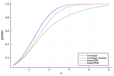
Figure 2: Local Asymptotic Power Curves under Thompson Sampling

The local asymptotic power curve of the ZJM test in Figure 2 is reasonably close to the limited power envelope for tests based on $(W_{1},W_{2})$ for small values of the alternative, with a slight gap for intermediate values. The pooled difference in means test, however, has higher power uniformly across the space of alternatives, and exceeds the power envelope for tests based on $(W_{1},W_{2})$. This suggests that restricting the test to only use the batchwise differences in means $W_{1}$ and $W_{2}$ may entail a nontrivial loss in power. The pooled difference-in-means test has power very close to the full power envelope. It should be pointed out that these results hold for a specific choice of the arm-specific variances $\sigma_{0}^{2}$ and $\sigma_{1}^{2}$ and for this specific scenario with two equally-sized batches. Further work could examine the performance of these tests under a variety of setups and seek to draw more general recommendations for testing procedures with robust power properties.

Our representation result also allows us to consider, and compare, alternative choices for the adaptive treatment assignment rule. Some authors, including Kasy and Sautmann (2021) and Caria, Gordon, Kasy, Quinn, Shami, and Teytelboym (2020), have suggested modifying the Thompson sampling rule to make the chosen treatment probabilities closer to equality across arms. Intuitively, bandit algorithms such as Thompson sampling target in-sample allocative efficiency, at the possible expense of efficiency for statistical inference about population parameters. Shrinking towards a balanced allocation could result in better power for tests of hypotheses about treatment effects.

As a simple illustration, we consider a weighted allocation rule

$$\Lambda_{2,c}(Z_{1})=(1-c)\Lambda_{2}(Z_{1})+c(1/2),\quad c\in[0,1],$$

which shrinks the (asymptotic) Thompson sampling rule towards a 50-50 treatment rule.

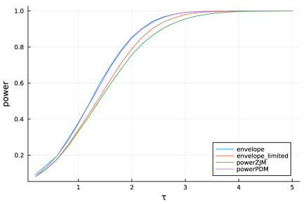
Figure 3: Weighted Thompson Rule, $c=0.1$

Figure 3 considers the case where $c=0.1$. It shows that, even with a fairly mild degree of shrinkage, the differences between the power functions become smaller, although the relative comparisons retain their orderings. As with the simulations shown in Figure 2, these results hold for a specific scenario, and warrant further exploration. The limiting Gaussian bandit representation provides a computationally tractable framework for examining and comparing alternative testing procedures for batched adaptive experimental designs.

5 Conclusion

The representation results we have developed in this paper characterize all attainable limit distributions of procedures in a rich class of dynamic statistical decision problems where the agent’s actions can include the choice of the adaptive experimentation rule. They do not require restricting attention to a specific class of rules, such as Bayes rules or empirical analog (plug-in) rules, and can be combined with any solution concept such as minmax regret or robust preferences. Decision problems that are intractable in their original form can be dramatically simplified through these approximations. However, whether or not the asymptotic approximation of the original problem by a limiting Gaussian bandit is simple enough to yield an explicit solution will depend on the specific problem at hand. For more complex problems, it may be useful to first apply our representation theorem, and then use numerical methods to obtain an approximate solution to the simplified decision problem.

Appendix A Proofs

Proof of Theorem 1:

Consider the vector of likelihood ratios:

$$\left\{\ell_{1,n}(h,h_{0}),\ell_{2,n}(h,h_{0}),\ell_{12,n}(h,h_{0})\right\}:=\left\{\prod_{\frac{i}{n}\in N_{1}}\frac{p_{\theta_{n}(h)}(z_{i})}{p_{\theta_{n}(h_{0})}(z_{i})},\prod_{\frac{i}{n}\in N_{2}}\frac{p_{\theta_{n}(h)}(z_{i})}{p_{\theta_{n}(h_{0})}(z_{i})},\prod_{\frac{i}{n}\in N_{12}}\frac{p_{\theta_{n}(h)}(z_{i})}{p_{\theta_{n}(h_{0})}(z_{i})}\right\}.$$

By the differentiability in quadratic mean condition in Assumption 1 and standard calculations, we have, for any local parameter $h_{0}$,

$$\left\{\ell_{1,n}(h,h_{0}),\ell_{2,n}(h,h_{0}),\ell_{12,n}(h,h_{0})\right\} \stackrel{{\scriptstyle h_{0}}}{{\leadsto}}\Biggl{\{}\exp\left(\sqrt{\lambda_{1}}(h-h_{0})^{\prime}\Delta_{1}-\frac{\lambda_{1}}{2}(h-h_{0})^{\prime}J(h-h_{0})\right),$$

$$\qquad\exp\left(\sqrt{\lambda_{2}}(h-h_{0})^{\prime}\Delta_{2}-\frac{\lambda_{2}}{2}(h-h_{0})^{\prime}J(h-h_{0})\right),$$

$$\qquad\exp\left(\sqrt{\lambda_{12}}(h-h_{0})^{\prime}\Delta_{12}-\frac{\lambda_{12}}{2}(h-h_{0})^{\prime}J(h-h_{0})\right)\Biggr{\}},$$

where $\Delta_{1},\Delta_{2},\Delta_{12}$ are independent copies of $N(0,J)$ random vectors. Note that the experiment

$$\begin{pmatrix}Z_{1}\\ Z_{2}\\ Z_{12}\end{pmatrix}\sim N\left(\begin{pmatrix}h\\ h\\ h\end{pmatrix},\begin{pmatrix}(\lambda_{1}J)^{-1}&&0\\ &(\lambda_{2}J)^{-1}&\\ 0&&(\lambda_{12}J)^{-1}\end{pmatrix}\right),$$

has the same likelihood ratios as the above limit.

The vectors $(S_{1,n},S_{2,n})$ and $(\ell_{1,n}(h,h_{0}),\ell_{2,n}(h,h_{0}),\ell_{12,n}(h,h_{0}))$ each converge marginally under $h_{0}=0$. By Prohorov’s theorem for random vectors in Euclidean spaces (van der Vaart, 1998, Theorem 2.4) these marginals are uniformly tight, and marginal tightness implies joint convergence along a subsequence. So, on this subsequence we have

$$\left\{S_{1,n},S_{2,n},\ell_{1,n}(h,0),\ell_{2,n}(h,0),\ell_{12,n}(h,0)\right\} \stackrel{{\scriptstyle 0}}{{\leadsto}}\Biggl{\{}S_{1},S_{2},\exp\left(\sqrt{\lambda_{1}}h^{\prime}\Delta_{1}-\frac{\lambda_{1}}{2}h^{\prime}Jh\right),$$

$$\quad\exp\left(\sqrt{\lambda_{2}}h^{\prime}\Delta_{2}-\frac{\lambda_{2}}{2}h^{\prime}Jh\right),\exp\left(\sqrt{\lambda_{12}}h^{\prime}\Delta_{12}-\frac{\lambda_{12}}{2}h^{\prime}Jh\right)\Biggr{\}}.$$

Recall that $\mathcal{L}_{h}$ is the joint law of $S_{1},S_{2}$ under $h$. By contiguity and Le Cam’s third lemma, for any Borel sets $B_{1}$ and $B_{2}$,

$$\mathcal{L}_{h}(B_{1}\times B_{2}) =E\Biggl{[}1(S_{1}\in B_{1})1(S_{2}\in B_{2})\exp\left(\sqrt{\lambda_{1}}h^{\prime}\Delta_{1}-\frac{\lambda_{1}}{2}h^{\prime}Jh\right)$$

$$\qquad\cdot\exp\left(\sqrt{\lambda_{2}}h^{\prime}\Delta_{2}-\frac{\lambda_{2}}{2}h^{\prime}Jh\right)\cdot\exp\left(\sqrt{\lambda_{12}}h^{\prime}\Delta_{12}-\frac{\lambda_{12}}{2}h^{\prime}Jh\right)\Biggr{]}.$$

Now, consider the joint random vector $(S_{1},S_{2},\Delta_{1},\Delta_{2},\Delta_{12})$. These limiting random variables will reflect their finite sample analogs in the sense that $S_{1}$ and $\Delta_{2}$ are independent conditional on $(\Delta_{1},\Delta_{12})$, and $S_{2}$ and $\Delta_{1}$ are independent conditional on $(\Delta_{2},\Delta_{12})$. That is,

$$S_{1}|\Delta_{1},\Delta_{2},\Delta_{12}\ \sim\ S_{1}|\Delta_{1},\Delta_{12}\hskip 28.45274pt\mbox{and}\hskip 28.45274ptS_{2}|\Delta_{1},\Delta_{2},\Delta_{12}\ \sim\ S_{2}|\Delta_{2},\Delta_{12}.$$ (3)

Next we construct the randomized experiments in the limit experiment corresponding to $S_{1,n},S_{2,n}$. We invoke Theorem 2.1 in Carlier, Chernozhukov, and Galichon (2016), which states that there exists a map

$$Q_{S_{1},S_{2}|\Delta_{1},\Delta_{2},\Delta_{12}}(u,\delta_{1},\delta_{2},\delta_{12})$$

with range $\mathbb{R}^{2}$ such that $Q_{S_{1},S_{2}|\Delta_{1},\Delta_{2},\Delta_{12}}(U,\delta_{1},\delta_{2},\delta_{12})$ has the distribution $S_{1},S_{2}|\Delta_{1}=\delta_{1},\Delta_{2}=\delta_{2},\Delta_{12}=\delta_{12}$, where $U$ is an independent standard uniform on the unit square, $U\sim U(0,1)^{2}$. Let

$$(\tilde{S}_{1},\tilde{S}_{2})=Q_{S_{1},S_{2}|\Delta_{1},\Delta_{2},\Delta_{12}}(U,\Delta_{1},\Delta_{2},\Delta_{12}).$$

Then, by construction,

$$(\tilde{S}_{1},\tilde{S}_{2},\Delta_{1},\Delta_{2},\Delta_{12})\sim(S_{1},S_{2},\Delta_{1},\Delta_{2},\Delta_{12}).$$

Moreover, Carlier, Chernuzhukov, and Galichon’s Theorem 2.1 states that we can choose $U$ such that

$$(\tilde{S}_{1},\tilde{S}_{2})=(S_{1},S_{2})\ \ \text{a.s.}$$

Let us examine what (3) implies about $Q_{S_{1},S_{2}|\Delta_{1},\Delta_{2},\Delta_{12}}(\cdot)$. Use the following notation for each element of $Q_{S_{1},S_{2}|\Delta_{1},\Delta_{2},\Delta_{12}}(\cdot)$:

$$\left(\begin{array}[]{c}\tilde{S}_{1}\\ \tilde{S}_{2}\end{array}\right)\ =\ \left(\begin{array}[]{c}Q^{1}_{S_{1},S_{2}|\Delta_{1},\Delta_{2},\Delta_{12}}(U,\Delta_{1},\Delta_{2},\Delta_{12})\\ Q^{2}_{S_{1},S_{2}|\Delta_{1},\Delta_{2},\Delta_{12}}(U,\Delta_{1},\Delta_{2},\Delta_{12})\end{array}\right).$$

Then (3) implies that $Q^{1}_{S_{1},S_{2}|\Delta_{1},\Delta_{2},\Delta_{12}}$ does not depend on $\Delta_{2}$ and $Q^{2}_{S_{1},S_{2}|\Delta_{1},\Delta_{2},\Delta_{12}}$ does not depend on $\Delta_{1}$. So, with some abuse of notation, we will write

$$\left(\begin{array}[]{c}\tilde{S}_{1}\\ \tilde{S}_{2}\end{array}\right)\ =\ \left(\begin{array}[]{c}Q^{1}_{S_{1},S_{2}|\Delta_{1},\Delta_{2},\Delta_{12}}(U,\Delta_{1},\Delta_{12})\\ Q^{2}_{S_{1},S_{2}|\Delta_{1},\Delta_{2},\Delta_{12}}(U,\Delta_{2},\Delta_{12})\end{array}\right).$$

This simplification is important because we will next construct the random variables with the correct distribution under any $h$, and these restrictions on $Q_{S_{1},S_{2}|\Delta_{1},\Delta_{2},\Delta_{12}}(\cdot)$ imply that the constructed random variables will inherit these conditional independence property for any $h$.

Recall that, under $h=0$,

$$\left(\begin{array}[]{c}\sqrt{\lambda_{1}}JZ_{1}\\ \sqrt{\lambda_{2}}JZ_{2}\\ \sqrt{\lambda_{12}}JZ_{12}\end{array}\right)\ \sim\ \left(\begin{array}[]{c}\Delta_{1}\\ \Delta_{2}\\ \Delta_{12}\end{array}\right).$$

Let

$$\left(\begin{array}[]{c}T_{1}\\ T_{2}\end{array}\right) = \left(\begin{array}[]{c}Q^{1}_{S_{1},S_{2}|\Delta_{1},\Delta_{2},\Delta_{12}}(U,\sqrt{\lambda_{1}}JZ_{1},\sqrt{\lambda_{12}}JZ_{12})\\ Q^{2}_{S_{1},S_{2}|\Delta_{1},\Delta_{2},\Delta_{12}}(U,\sqrt{\lambda_{2}}JZ_{2},\sqrt{\lambda_{12}}JZ_{12})\end{array}\right).$$

Finally, we verify that $(T_{1},T_{2})$ has the desired distribution for any value of $h$. For measurable sets $B_{1}$ and $B_{2}$,

$${\Pr}_{h}(T_{1}\in B_{1},T_{2}\in B_{2})$$

$$= {\Pr}_{h}(Q^{1}_{S_{1},S_{2}|\Delta_{1},\Delta_{2},\Delta_{12}}(U,\sqrt{\lambda_{1}}JZ_{1},\sqrt{\lambda_{12}}JZ_{12})\in B_{1},Q^{2}_{S_{1},S_{2}|\Delta_{1},\Delta_{2},\Delta_{12}}(U,\sqrt{\lambda_{2}}JZ_{2},\sqrt{\lambda_{12}}JZ_{12})\in B_{2})$$

$$= \int\int\int\Pr(Q^{1}_{S_{1},S_{2}|\Delta_{1},\Delta_{2},\Delta_{12}}(U,\sqrt{\lambda_{1}}Jz_{1},\sqrt{\lambda_{12}}Jz_{12})\in B_{1},Q^{2}_{S_{1},S_{2}|\Delta_{1},\Delta_{2},\Delta_{12}}(U,\sqrt{\lambda_{2}}Jz_{2},\sqrt{\lambda_{12}}Jz_{12})\in B_{2})$$

$$\hskip 28.45274pt\cdot\ \phi(z_{1}|h,(\lambda_{1}J)^{-1})\phi(z_{2}|h,(\lambda_{2}J)^{-1})\phi(z_{12}|h,(\lambda_{12}J)^{-1})dz_{1}dz_{2}dz_{12}$$

$$= \int\int\int\Pr(Q^{1}_{S_{1},S_{2}|\Delta_{1},\Delta_{2},\Delta_{12}}(U,\sqrt{\lambda_{1}}Jz_{1},\sqrt{\lambda_{12}}Jz_{12})\in B_{1},Q^{2}_{S_{1},S_{2}|\Delta_{1},\Delta_{2},\Delta_{12}}(U,\sqrt{\lambda_{2}}Jz_{2},\sqrt{\lambda_{12}}Jz_{12})\in B_{2})$$

$$\hskip 28.45274pt\cdot\ \frac{\phi(z_{1}|h,(\lambda_{1}J)^{-1})}{\phi(z_{1}|0,(\lambda_{1}J)^{-1})}\frac{\phi(z_{2}|h,(\lambda_{2}J)^{-1})}{\phi(z_{2}|0,(\lambda_{2}J)^{-1})}\frac{\phi(z_{12}|h,(\lambda_{12}J)^{-1})}{\phi(z_{12}|0,(\lambda_{12}J)^{-1})}$$

$$\hskip 28.45274pt\cdot\ \phi(z_{1}|0,(\lambda_{1}J)^{-1})\phi(z_{2}|0,(\lambda_{2}J)^{-1})\phi(z_{12}|0,(\lambda_{12}J)^{-1})dz_{1}dz_{2}dz_{12}$$

$$= E_{0}\left[{\bf 1}\{Q^{1}_{S_{1},S_{2}|\Delta_{1},\Delta_{2},\Delta_{12}}(U,\sqrt{\lambda_{1}}JZ_{1},\sqrt{\lambda_{12}}JZ_{12})\in B_{1},Q^{2}_{S_{1},S_{2}|\Delta_{1},\Delta_{2},\Delta_{12}}(U,\sqrt{\lambda_{2}}JZ_{2},\sqrt{\lambda_{12}}JZ_{12})\in B_{2}\}\right.$$

$$\hskip 28.45274pt\cdot\ \exp\left(\sqrt{\lambda_{1}}h^{\prime}(\sqrt{\lambda_{1}}JZ_{1})-\frac{\lambda_{1}}{2}h^{\prime}Jh\right)\cdot\exp\left(\sqrt{\lambda_{2}}h^{\prime}(\sqrt{\lambda_{2}}JZ_{2})-\frac{\lambda_{2}}{2}h^{\prime}Jh\right)$$

$$\hskip 28.45274pt\cdot\ \left.\exp\left(\sqrt{\lambda_{12}}h^{\prime}(\sqrt{\lambda_{12}}JZ_{12})-\frac{\lambda_{12}}{2}h^{\prime}Jh\right)\right]$$

$$= E\left[{\bf 1}\{S_{1}\in B_{1},S_{2}\in B_{2}\}\right.$$

$$\hskip 19.91684pt\cdot\ \left.\exp\left(\sqrt{\lambda_{1}}h^{\prime}\Delta_{1}-\frac{\lambda_{1}}{2}h^{\prime}Jh\right)\cdot\exp\left(\sqrt{\lambda_{2}}h^{\prime}\Delta_{2}-\frac{\lambda_{2}}{2}h^{\prime}Jh\right)\cdot\ \exp\left(\sqrt{\lambda_{12}}h^{\prime}\Delta_{12}-\frac{\lambda_{12}}{2}h^{\prime}Jh\right)\right]$$

$$= \mathcal{L}_{h}(B_{1}\times B_{2}).$$

We conclude that $(T_{1},T_{2})$ satisfies the statement of the theorem.

$\Box$

Proof of Corollary 2:

First note that the extension of Theorem 1 to $D>2$ fixed information sets is straightforward.

For notational ease, set the parameter dimension to be $m=1$ and set $J_{0}=1$. The case for general $m$ and $J_{0}$ follows with obvious modifications. We are given $t_{1},t_{2},\dots,t_{D}$ with $0<t_{1}<\cdots<t_{D}\leq 1$, and information sets $I_{d}=[0,t_{d}]$ for $d=1,\dots,D$, so that

$$I_{1}\subset I_{2}\subset\cdots\subset I_{D}.$$

The non-overlapping subsets can be written as

$$I_{1} =[0,t_{1}],$$

$$N_{2} =I_{2}\setminus I_{1}=(t_{1},t_{2}],$$

$$N_{3} =I_{3}\setminus I_{2}=(t_{2},t_{3}],$$

and so on. By Theorem 1, a limit experiment can be expressed as

$$Z=\begin{pmatrix}Z_{1}\\ \vdots\\ Z_{D}\end{pmatrix}\sim N\left(\begin{pmatrix}h\\ \vdots\\ h\end{pmatrix},\Omega\right),\quad\Omega=\text{diag}\left\{\frac{1}{t_{1}},\frac{1}{t_{2}-t_{1}},\dots,\frac{1}{t_{D}-t_{D-1}}\right\},$$

with some $U\perp Z$, and there exists a collection of functions $T_{1},\dots,T_{D}$ with

$$T=\begin{pmatrix}T_{1}(Z_{1},U)\\ T_{2}(Z_{1},Z_{2},U)\\ \vdots\\ T_{D}(Z_{1},\dots,Z_{D},U)\end{pmatrix}\sim\mathcal{L}_{h},\quad\forall h.$$

First consider the case with $D=2$, so the limit experiment can be written as

$$Z=\begin{pmatrix}Z_{1}\\ Z_{2}\end{pmatrix}\sim N\left(\begin{pmatrix}h\\ h\end{pmatrix},\begin{bmatrix}\frac{1}{t_{1}}&0\\ 0&\frac{1}{t_{2}-t_{1}}\end{bmatrix}\right),\quad U\perp Z,$$

and the corresponding statistics are

$$\begin{pmatrix}T_{1}(Z_{1},U)\\ T_{2}(Z_{1},Z_{2},U)\end{pmatrix}\sim\mathcal{L}_{h}.$$

Let $B(t)$ be a standard Brownian motion on $t\in[0,1]$ and let $W(t)=th+B(t)$. If we construct

$$\tilde{Z}_{1} =\frac{1}{t_{1}}W(t_{1}),$$

$$\tilde{Z}_{2} =\frac{1}{t_{2}-t_{1}}\left[W(t_{2})-W(t_{1})\right],$$

then $(\tilde{Z}_{1},\tilde{Z}_{2})$ is equal in distribution to $(Z_{1},Z_{2})$. Now define

$$\tilde{T}_{1}(w_{1},u) =T_{1}\left(\frac{1}{t_{1}}w_{1},u\right).$$

$$\tilde{T}_{2}(w_{1},w_{2},u) =T_{2}\left(\frac{1}{t_{1}}w_{1},\frac{1}{t_{2}-t_{1}}[w_{2}-w_{1}],u\right).$$

Then

$$\tilde{T}=\begin{pmatrix}\tilde{T}_{1}(W(t_{1}),U)\\ \tilde{T}_{2}(W(t_{1}),W(t_{2}),U)\end{pmatrix}\sim T\sim\mathcal{L}_{h}.$$

Next, we want to show that we can express $\tilde{T}_{2}$ as a function only of $W(t_{2})$, $U$, and some other variable independent of $W(t_{2})$. Define

$$V(t)=B(t)-\frac{t}{t_{D}}B(t_{D}),\quad 0\leq t\leq t_{D},$$

where $B(t)$ is the Brownian motion in the definition of $W(t)$. The process $V(\cdot)$ is a Brownian bridge, and a standard fact is that $V(\cdot)$ is independent of the endpoint $B(t_{D})$. This implies that for any $t$ and any $h$, $V(t)$ is independent of $W(t_{D})$.

Focusing first on the case with $D=2$, from the definition of $V(t)$ we can write

$$B(t_{1})=\frac{t_{1}}{t_{2}}B(t_{2})+V(t_{1}),$$

so that

$$W(t_{1}) =t_{1}h+B(t_{1})$$

$$=t_{1}h+\frac{t_{1}}{t_{2}}B(t_{2})+V(t_{1})$$

$$=t_{1}h+\frac{t_{1}}{t_{2}}[W(t_{2})-t_{2}h]+V(t_{1})$$

$$=\frac{t_{1}}{t_{2}}W(t_{2})+V(t_{1}).$$

Next, define

$$\widehat{T}_{2}(w_{2},v,u)=\tilde{T}_{2}\left(\frac{t_{1}}{t_{2}}w_{2}+v,w_{2},u\right).$$

Then

$$\widehat{T}_{2}(W(t_{2}),V(t_{1}),U)=\tilde{T}_{2}\left(W(t_{1}),W(t_{2}),U\right).$$

Therefore,

$$\begin{pmatrix}\tilde{T}_{1}(W(t_{1}),U)\\ \widehat{T}_{2}(W(t_{2}),V(t_{1}),U)\end{pmatrix}=\tilde{T}\sim T\sim\mathcal{L}_{h}.$$

Note that $V(t_{1})$ is independent of $W(t_{2})$, but not of $W(t_{1})$.

For $D>2$, we can construct the alternative representations in a similar way. For $d=1,\dots,D$, we can construct copies of the $Z_{d}$ from $W(t_{1})$ through $W(t_{d})$ as

$$\tilde{Z}_{d}=\frac{1}{t_{d}-t_{d-1}}\left[W(t_{d})-W(t_{d-1})\right],$$

and define $\tilde{T}_{1},\dots,\tilde{T}_{D}$ appropriately so that

$$\tilde{T}=\begin{pmatrix}\tilde{T}_{1}(W(t_{1}),U)\\ \tilde{T}_{2}(W(t_{1}),W(t_{2}),U)\\ \vdots\\ \tilde{T}_{D}(W(t_{1}),\dots,W(t_{D}),U)\end{pmatrix}\sim\mathcal{L}_{h}.$$

To construct the representation in terms of the Brownian bridge, note that for any $d=1,\dots,D$, we have

$$W(t_{d}) =t_{d}h+B(t_{d})$$

$$=\frac{t_{d}}{t_{D}}W(t_{D})+V(t_{d}),$$

so that

$$W(t_{D})=\frac{t_{D}}{t_{d}}\left[W(t_{d})-V(t_{d})\right].$$

Now, consider any $c<d$. We can write

$$W(t_{c}) =\frac{t_{c}}{t_{D}}W(t_{D})+V(t_{c})$$

$$=\frac{t_{c}}{t_{D}}\frac{t_{D}}{t_{d}}\left[W(t_{d})-V(t_{d})\right]+V(t_{c}).$$

Thus, for any $1<d\leq D$ we can reconstruct $W(t_{1}),\dots,W(t_{d})$ from $W(t_{d}),V(t_{1}),\dots,V(t_{d})$. So we can construct functions

$$\widehat{T}_{d}(W(t_{d}),V(t_{1}),\dots,V(t_{d}),U)=\tilde{T}_{d}(W(t_{1}),\dots,W(t_{d}),U).$$

For $d=1$, we can set $\widehat{T}_{1}=\tilde{T}_{1}$. For $d=D$, we have $V(t_{D})=0$ by construction, so it suffices to know $W(t_{D}),V(t_{1}),\dots,V(t_{D-1})$ to construct $W(t_{1}),\dots,W(t_{D})$.

$\Box$

Proof of Theorem 3:

The first step will be to characterize the asymptotic behavior of the likelihood ratio process. For each sample observation, we have both the observed arm data and the “potential” data on unobserved arms. It will be useful to jointly characterize both the likelihood ratio process corresponding to the observed data and the “potential” likelihood ratio process corresponding to data from all arms including the unobserved potential arm data. Without loss of generality, we specify an auxiliary model of unobserved arm data that will exactly preserve the finite sample behavior of the observed data and maintain the assumptions of the theorem. In the auxiliary model, the marginal distribution of data associated with each arm, $p^{(b)}_{\theta,k}(z_{b,i}(k))$, will remain as provided in the supposition of the theorem, and we will additionally take $z_{b,i}(0),\ldots,z_{b,i}(K-1)$ to be independent (across arms). By construction, both the auxiliary potential likelihood and the “actual” potential likelihood will generate identical likelihoods for the observable data. Note that, in the proof to follow, the “potential” likelihood will be a reference to the likelihood of observed and unobserved data for the auxiliary model.

Given $\lambda_{b}=(\lambda_{b,0},\ldots,\lambda_{b,K})$ for batch $b\in\{1,\ldots,B\}$, the (observed data) likelihood ratio process of $\theta_{n}(h)=\theta_{0}+h/\sqrt{n}$ versus $\theta_{0}$ is given by

$$\ell_{b,n}(h;\lambda_{b})=\prod_{k=0}^{K-1}\prod_{i=\lfloor n\lambda_{b,k}\rfloor+1}^{\lfloor n\lambda_{b,k+1}\rfloor}\frac{p^{(b)}_{\theta_{n}(h),k}(z_{b,i}(k))}{p^{(b)}_{\theta_{0},k}(z_{b,i}(k))}$$

for all $h\in\mathbb{R}^{m}$, and for batch $b\in\{2,\ldots,B\}$, we take the the auxiliary (unobserved data) likelihood ratio process of $\theta_{n}(h)=\theta_{0}+h/\sqrt{n}$ versus $\theta_{0}$ to be given by

$$\ell_{b,n}^{-}(h;\lambda_{b})=\prod_{k=0}^{K-1}\prod_{\begin{subarray}{c}1\leq i\leq\lfloor n\lambda_{b,k}\rfloor\\ \lfloor n\lambda_{b,k+1}\rfloor+1\leq i\leq\lfloor n\bar{\lambda}_{b}\rfloor\end{subarray}}\frac{p^{(b)}_{\theta_{n}(h),k}(z_{b,i}(k))}{p^{(b)}_{\theta_{0},k}(z_{b,i}(k))}$$

for all $h\in\mathbb{R}^{m}$. Note that, for observation $i$, this specification imposes independence across arms. Also, we focus only on batches $\{2,\ldots,B\}$ where the observed arms are determined adaptively.

Jointly over batches, these likelihood ratio processes form stochastic processes in $(\lambda_{1},\ldots,\lambda_{B})$:

$$\ell_{n}(h)(\lambda_{1},\ldots,\lambda_{B})=(\ell_{1,n}(h;\lambda_{1}),\ldots,\ell_{B,n}(h;\lambda_{B}))$$

and

$$\ell_{n}^{-}(h)(\lambda_{2},\ldots,\lambda_{B})=(\ell_{2,n}^{-}(h;\lambda_{2}),\ldots,\ell_{B,n}^{-}(h;\lambda_{B})).$$

Under the DQM assumption and Donsker’s Theorem for partial-sum processes (e.g. van der Vaart and Wellner, 1996, Theorem 2.12.6), the pair $(\ell_{n}(h),\ell_{n}^{-}(h))$ converges weakly to a tight random element:

$$(\ell_{n}(h),\ell_{n}^{-}(h))\stackrel{{\scriptstyle\theta_{0}}}{{\leadsto}}(\ell^{0}(h),\ell^{0-}(h)),$$ (5)

where

$$\ell^{0}(h )(\lambda_{1},\ldots,\lambda_{B})$$ (6)

$$= \left(\prod_{k=0}^{K-1}\exp\left[h^{\prime}(\Delta_{1,k}(\lambda_{1,k+1})-\Delta_{1,k}(\lambda_{1,k}))-\frac{(\lambda_{1,k+1}-\lambda_{1,k})}{2}h^{\prime}J_{k}^{(1)}h\right],\ldots,\right.$$

$$\left.\ \ \ \prod_{k=0}^{K-1}\exp\left[h^{\prime}(\Delta_{B,k}(\lambda_{B,k+1})-\Delta_{B,k}(\lambda_{B,k}))-\frac{(\lambda_{B,k+1}-\lambda_{B,k})}{2}h^{\prime}J_{k}^{(B)}h\right]\right),$$

$$\ell^{0-} (h)({\lambda}_{2},\ldots,\lambda_{B})$$ (7)

$$= \left(\prod_{k=0}^{K-1}\exp\left[h^{\prime}[(\Delta_{2,k}(\bar{\lambda}_{2})-\Delta_{2,k}(\lambda_{2,k+1}))+(\Delta_{2,k}(\lambda_{2,k})-\Delta_{2,k}(\lambda_{2,0}))]-\frac{(\bar{\lambda}_{2}-\lambda_{2,k+1}+\lambda_{2,k})}{2}h^{\prime}J_{k}^{(2)}h\right],\ldots,\right.$$

$$\left.\ \ \ \prod_{k=0}^{K-1}\exp\left[h^{\prime}[(\Delta_{B,k}(\bar{\lambda}_{B})-\Delta_{B,k}(\lambda_{B,k+1}))+(\Delta_{B,k}(\lambda_{B,k})-\Delta_{B,k}(\lambda_{B,0}))]-\frac{(\bar{\lambda}_{B}-\lambda_{B,k+1}+\lambda_{B,k})}{2}h^{\prime}J_{k}^{(B)}h\right]\right),$$

and the $\Delta_{b,k}(\cdot)$ are Gaussian processes with independent increments such that $\Delta_{b,k}(t)\sim N(0,tJ_{k}^{(b)})$ for $t\geq 0$, with independence across $b$ and $k$.

Putting together the observed and unobserved likelihood ratios, we can denote the “potential” likelihood ratio for batch $b\in\{2,\ldots,B\}$ by

$$\bar{\ell}_{b,n}(h)=\prod_{k=0}^{K-1}\prod_{i=1}^{\lfloor n\bar{\lambda}_{b}\rfloor}\frac{p^{(b)}_{\theta_{n}(h),k}(z_{b,i}(k))}{p^{(b)}_{\theta_{0},k}(z_{b,i}(k))},$$

and form the joint likelihood over these batches: $\bar{\ell}_{n}(h)=(\bar{\ell}_{2,n}(h),\ldots,\bar{\ell}_{B,n}(h))$. Note that $\bar{\ell}_{b,n}(h)=\ell_{b,n}(h;\lambda_{b})\cdot\ell_{b,n}^{-}(h;\lambda_{b})$, but $\bar{\ell}_{b,n}(h)$ does not depend on $\lambda_{b}$. The weak limit of $\bar{\ell}_{n}(h)$ will be used for Le Cam’s third lemma below, and this limit follows by (5),

$$\bar{\ell}_{n}(h)\stackrel{{\scriptstyle\theta_{0}}}{{\leadsto}}\bar{\ell}^{0}(h),$$

where

$$\bar{\ell}^{0}(h)=\left(\prod_{k=0}^{K-1}\exp\left[h^{\prime}\Delta_{2,k}(\bar{\lambda}_{2})-\frac{\bar{\lambda}_{2}}{2}h^{\prime}J_{k}^{(2)}k\right],\ldots,\prod_{k=0}^{K-1}\exp\left[h^{\prime}\Delta_{B,k}(\bar{\lambda}_{B})-\frac{\bar{\lambda}_{B}}{2}h^{\prime}J_{k}^{(B)}h\right]\right).$$ (8)

For batch 1, $\lambda_{1}$ determines the observations from each arm. Let

$$\Delta_{1}(\lambda_{1})\,=\,\left(\Delta_{1,0}(\lambda_{1,1})-\Delta_{1,0}(\lambda_{1,0}),\ldots,\Delta_{1,K-1}(\lambda_{1,K})-\Delta_{1,K-1}(\lambda_{1,K-1})\right).$$

For batches $2,\ldots,B$, the scores $\Delta_{b,k}(\bar{\lambda}_{b})$ from (8), which represent the limiting potential information from batch $b$ and arm $k$, can be partitioned into “observed” and “unobserved” scores (see (6) and (7)) as determined by $(\lambda_{b,k},\lambda_{b,k+1})$:

$$\Delta_{b}(\lambda_{b}) \,=\,\left(\Delta_{b,0}(\lambda_{b,1})-\Delta_{b,0}(\lambda_{b,0}),\ldots,\Delta_{b,K-1}(\lambda_{b,K})-\Delta_{b,K-1}(\lambda_{b,K-1})\right);$$

$$\Delta_{b}^{-}(\lambda_{b}) \,=\,\left(\Delta_{b,0}(\bar{\lambda}_{b})-\Delta_{b,0}(\lambda_{b,1}),\Delta_{b,1}(\lambda_{b,1})-\Delta_{b,1}(\lambda_{b,0}),\Delta_{b,1}(\bar{\lambda}_{b})-\Delta_{b,1}(\lambda_{b,2}),\ldots,\right.$$

$$\hskip 54.06006pt\left.\Delta_{b,K-1}(\lambda_{b,K-1})-\Delta_{b,K-1}(\lambda_{b,0}),\Delta_{b,K-1}(\bar{\lambda}_{b})-\Delta_{b,K-1}(\lambda_{b,K})\right);$$

$$\bar{\Delta}_{b} \,=\,\left(\Delta_{b,0}(\bar{\lambda}_{b}),\ldots,\Delta_{b,K-1}(\bar{\lambda}_{b})\right).$$

Note that, for any $\lambda_{b}$, $\Delta_{b}(\lambda_{b})$ and $\Delta_{b}^{-}(\lambda_{b})$ are independent.

By supposition, the statistics $S_{b,n}$ and $\Lambda_{b,n}$ jointly converge weakly under $\theta_{0}$. For convenience, we use zero superscripts to denote their limits, and write

$$\left(S_{1,n},\Lambda_{2,n},S_{2,n},\dots,\Lambda_{B,n},S_{B,n}\right)\ \stackrel{{\scriptstyle\theta_{0}}}{{\leadsto}}\ \left(S_{1}^{0},\Lambda_{2}^{0},S_{2}^{0},\dots,\Lambda_{B}^{0},S_{B}^{0},\right).$$

Prohorov’s Theorem (van der Vaart and Wellner, 1996, Theorem 1.3.9) and auxiliary results (van der Vaart and Wellner, 1996, Lemmas 1.4.3 and 1.4.4) imply that along a subsequence we have joint convergence of the statistics and the likelihood ratio processes,

$$\left(S_{1,n},\Lambda_{2,n},S_{2,n},\dots,\Lambda_{B,n},S_{B,n},\ell_{n}(h),\bar{\ell}_{n}(h)\right)\ \stackrel{{\scriptstyle\theta_{0}}}{{\leadsto}}\ \left(S_{1}^{0},\Lambda_{2}^{0},S_{2}^{0},\dots,\Lambda_{B}^{0},S_{B}^{0},\ell^{0}(h),\bar{\ell}^{0}(h)\right),$$

for each $h\in\mathbb{R}^{m}$.

Next we construct representations for the weak limit of the statistics under $\theta_{0}$. The constructions will rely on conditional vector quantile functions. Given two random vectors $Y$ and $X$ taking values on $\mathbb{R}^{d_{Y}}$ and $\mathbb{R}^{d_{X}}$, the conditional vector quantile function of $Y$ given $X=x$ can be defined as a map $u\mapsto q_{Y|X}(u|x)$ where $u$ takes values on the $\mathbb{R}^{d_{Y}}$ unit cube and $q_{Y|X}(U|x)$ has the distribution of $Y$ conditional on $X=x$ when $U$ is uniformly distributed on the $\mathbb{R}^{d_{Y}}$ unit cube (Carlier, Chernozhukov, and Galichon, 2016).

Our construction proceeds recursively. Let $U_{1},\ldots,U_{B}$ be independent uniformly distributed random vectors on the appropriate unit cube that are also independent of $\left(\Delta_{b,k}\right)_{b=1,k=0}^{B,K-1}$.

1. Given the conditional vector quantile function $q_{(S_{1}^{0},\Lambda_{2}^{0})|\Delta_{1}(\lambda_{1})}(u|\delta_{1})$, define

   $$(Q_{S_{1}^{0}},Q_{\Lambda_{2}^{0}})=q_{(S_{1}^{0},\Lambda_{2}^{0})|\Delta_{1}(\lambda_{1})}(U_{1}|\Delta_{1}(\lambda_{1})).$$

   Then,

   $$(\Delta_{1}(\lambda_{1}),Q_{S_{1}^{0}},Q_{\Lambda_{2}^{0}})\sim(\Delta_{1}(\lambda_{1}),S_{1}^{0},\Lambda_{2}^{0}).$$

2. Note that $(\Delta_{2,0},\ldots,\Delta_{2,K-1})\perp(\Delta_{1}(\lambda_{1}),Q_{S_{1}^{0}},Q_{\Lambda_{2}^{0}})$ and $(\Delta_{2,0},\ldots,\Delta_{2,K-1})\perp(\Delta_{1}(\lambda_{1}),S_{1}^{0},\Lambda_{2}^{0})$. Hence, for the randomly stopped processes, $\Delta_{2}(Q_{\Lambda_{2}^{0}}),\Delta_{2}^{-}(Q_{\Lambda_{2}^{0}}),\Delta_{2}(\Lambda_{2}^{0}),\Delta_{2}^{-}(\Lambda_{2}^{0})$, we have

   $$(\Delta_{1}(\lambda_{1}),Q_{S_{1}^{0}},Q_{\Lambda_{2}^{0}},\Delta_{2}(Q_{\Lambda_{2}^{0}})) \sim(\Delta_{1}(\lambda_{1}),S_{1}^{0},\Lambda_{2}^{0},\Delta_{2}(\Lambda_{2}^{0}))\ \ \mbox{and}$$

   $$(\Delta_{1}(\lambda_{1}),Q_{S_{1}^{0}},Q_{\Lambda_{2}^{0}},\Delta_{2}^{-}(Q_{\Lambda_{2}^{0}})) \sim(\Delta_{1}(\lambda_{1}),S_{1}^{0},\Lambda_{2}^{0},\Delta_{2}^{-}(\Lambda_{2}^{0}))$$

   Since $\Delta_{2}(Q_{\Lambda_{2}^{0}})\perp\Delta_{2}^{-}(Q_{\Lambda_{2}^{0}})|\Delta_{1}(\lambda_{1}),Q_{S_{1}^{0}},Q_{\Lambda_{2}^{0}}$ and $\Delta_{2}(\Lambda_{2}^{0})\perp\Delta_{2}^{-}(\Lambda_{2}^{0})|\Delta_{1}(\lambda_{1}),S_{1}^{0},\Lambda_{2}^{0}$, it follows that

   $$(\Delta_{1}(\lambda_{1}),Q_{S_{1}^{0}},Q_{\Lambda_{2}^{0}},\Delta_{2}(Q_{\Lambda_{2}^{0}}),\Delta_{2}^{-}(Q_{\Lambda_{2}^{0}}))\sim(\Delta_{1}(\lambda_{1}),S_{1}^{0},\Lambda_{2}^{0},\Delta_{2}(\Lambda_{2}^{0}),\Delta_{2}^{-}(\Lambda_{2}^{0}))$$

3. For $b=2,\ldots,B-1$, given $(\Delta_{1}(\lambda_{1}),Q_{S_{1}^{0}},Q_{\Lambda_{2}^{0}},\Delta_{2}(Q_{\Lambda_{2}^{0}}),\ldots,Q_{S_{b-1}^{0}},Q_{\Lambda_{b}^{0}},\Delta_{b}(Q_{\Lambda_{b}^{0}}))$, we construct $(Q_{S_{b}^{0}},Q_{\Lambda_{b+1}^{0}})$ using the conditional vector quantile function
   $q_{(S_{b}^{0},\Lambda_{b+1}^{0})|\Delta_{1}(\lambda_{1}),S_{1}^{0},\Lambda_{2}^{0},\Delta_{2}(\Lambda_{2}^{0}),\ldots,S_{b-1}^{0},\Lambda_{b}^{0},\Delta_{b}(\Lambda_{b}^{0})}(u|\delta_{1},s_{1},\lambda_{2},\delta_{2},\ldots,s_{b-1},\lambda_{b},\delta_{b})$. Define

   $$(Q_{S_{b}^{0}},Q_{\Lambda_{b+1}^{0}})=$$

   $$q_{(S_{b}^{0},\Lambda_{b+1}^{0})|\Delta_{1}(\lambda_{1}),S_{1}^{0},\Lambda_{2}^{0},\Delta_{2}(\Lambda_{2}^{0}),\ldots,S_{b-1}^{0},\Lambda_{b}^{0},\Delta_{b}(\Lambda_{b}^{0})}(U_{b}|\Delta_{1}(\lambda_{1}),Q_{S_{1}^{0}},Q_{\Lambda_{2}^{0}},\Delta_{2}(Q_{\Lambda_{2}^{0}}),\ldots,Q_{S_{b-1}^{0}},Q_{\Lambda_{b}^{0}},\Delta_{b}(Q_{\Lambda_{b}^{0}})).$$

   Then,

   $$(\Delta_{1}(\lambda_{1}),Q_{S_{1}^{0}},Q_{\Lambda_{2}^{0}},\Delta_{2}(Q_{\Lambda_{2}^{0}}),\ldots,Q_{S_{b}^{0}},Q_{\Lambda_{b+1}^{0}})\,\sim\,(\Delta_{1}(\lambda_{1}),S_{1}^{0},\Lambda_{2}^{0},\Delta_{2}({\Lambda_{2}^{0}}),\ldots,{S_{b}^{0}},{\Lambda_{b+1}^{0}}).$$

   For $b\geq 3$, note that $U_{b}\perp(\Delta_{2}^{-}(Q_{\Lambda_{2}^{0}}),\ldots,\Delta_{b}^{-}(Q_{\Lambda_{b}^{0}}))$ $|\,\Delta_{1}(\lambda_{1}),Q_{S_{1}^{0}},Q_{\Lambda_{2}^{0}},\Delta_{2}(Q_{\Lambda_{2}^{0}}),\ldots,Q_{S_{b-1}^{0}},Q_{\Lambda_{b}^{0}},\Delta_{b}(Q_{\Lambda_{b}^{0}})$, and $({S_{b}^{0}},{\Lambda_{b+1}^{0}})\perp(\Delta_{2}^{-}({\Lambda_{2}^{0}}),\ldots,\Delta_{b}^{-}({\Lambda_{b}^{0}}))$ $|\,\Delta_{1}(\lambda_{1}),S_{1}^{0},\Lambda_{2}^{0},\Delta_{2}({\Lambda_{2}^{0}}),\ldots S_{b-1}^{0},\Lambda_{b}^{0},\Delta_{b}(\Lambda_{b}^{0})$. So,

   $$(Q_{S_{b}^{0}},Q_{\Lambda_{b+1}^{0}})\,|\,\Delta_{1}(\lambda_{1}),Q_{S_{1}^{0}},Q_{\Lambda_{2}^{0}},\Delta_{2}(Q_{\Lambda_{2}^{0}}),\Delta_{2}^{-}(Q_{\Lambda_{2}^{0}}),\ldots,Q_{S_{b-1}^{0}},Q_{\Lambda_{b}^{0}},\Delta_{b}(Q_{\Lambda_{b}^{0}}),\Delta_{b}^{-}(Q_{\Lambda_{b}^{0}})$$

   $$\sim\,(Q_{S_{b}^{0}},Q_{\Lambda_{b+1}^{0}})\,|\,\Delta_{1}(\lambda_{1}),Q_{S_{1}^{0}},Q_{\Lambda_{2}^{0}},\Delta_{2}(Q_{\Lambda_{2}^{0}}),\ldots,Q_{S_{b-1}^{0}},Q_{\Lambda_{b}^{0}},\Delta_{b}(Q_{\Lambda_{b}^{0}})$$

   $$\sim\,(S_{b}^{0},\Lambda_{b+1}^{0})\,|\,\Delta_{1}(\lambda_{1}),S_{1}^{0},\Lambda_{2}^{0},\Delta_{2}(\Lambda_{2}^{0}),\ldots,S_{b-1}^{0},\Lambda_{b}^{0},\Delta_{b}(\Lambda_{b}^{0})$$

   $$\sim\,(S_{b}^{0},\Lambda_{b+1}^{0})\,|\,\Delta_{1}(\lambda_{1}),S_{1}^{0},\Lambda_{2}^{0},\Delta_{2}(\Lambda_{2}^{0}),\Delta_{2}^{-}(\Lambda_{2}^{0}),\ldots,S_{b-1}^{0},\Lambda_{b}^{0},\Delta_{b}(\Lambda_{b}^{0}),\Delta_{b}^{-}(\Lambda_{b}^{0})$$

   and

   $$(\Delta_{1}(\lambda_{1}),Q_{S_{1}^{0}},Q_{\Lambda_{2}^{0}},\Delta_{2}(Q_{\Lambda_{2}^{0}}),\Delta_{2}^{-}(Q_{\Lambda_{2}^{0}}),\ldots,Q_{S_{b-1}^{0}},Q_{\Lambda_{b}^{0}},\Delta_{b}(Q_{\Lambda_{b}^{0}}),\Delta_{b}^{-}(Q_{\Lambda_{b}^{0}}),Q_{S_{b}^{0}},Q_{\Lambda_{b+1}^{0}})$$

   $$\sim\,(\Delta_{1}(\lambda_{1}),S_{1}^{0},\Lambda_{2}^{0},\Delta_{2}(\Lambda_{2}^{0}),\Delta_{2}^{-}(\Lambda_{2}^{0}),\ldots,S_{b-1}^{0},\Lambda_{b}^{0},\Delta_{b}(\Lambda_{b}^{0}),\Delta_{b}^{-}(\Lambda_{b}^{0}),S_{b}^{0},\Lambda_{b+1}^{0})$$

4. Note that $(\Delta_{b+1,0},\ldots,\Delta_{b+1,K-1})\perp(\Delta_{1}(\lambda_{1}),Q_{S_{1}^{0}},Q_{\Lambda_{2}^{0}},\Delta_{2}(Q_{\Lambda_{2}^{0}}),\Delta_{2}^{-}(Q_{\Lambda_{2}^{0}}),\ldots,Q_{S_{b}^{0}},Q_{\Lambda_{b+1}^{0}})$ and
   $(\Delta_{b+1,0},\ldots,\Delta_{b+1,K-1})\perp(\Delta_{1}(\lambda_{1}),S_{1}^{0},\Lambda_{2}^{0},\Delta_{2}({\Lambda_{2}^{0}}),\Delta_{2}^{-}(\Lambda_{2}^{0}),\ldots,{S_{b}^{0}},{\Lambda_{b+1}^{0}})$. Hence, for the randomly stopped processes, $\Delta_{b+1}(Q_{\Lambda_{b+1}^{0}})$, $\Delta_{b+1}^{-}(Q_{\Lambda_{b+1}^{0}})$, $\Delta_{b+1}({\Lambda_{b+1}^{0}})$, $\Delta_{b+1}^{-}({\Lambda_{b+1}^{0}})$, we have

   $$(\Delta_{1}(\lambda_{1}),Q_{S_{1}^{0}},Q_{\Lambda_{2}^{0}},\Delta_{2}(Q_{\Lambda_{2}^{0}}),\Delta_{2}^{-}(Q_{\Lambda_{2}^{0}}),\ldots,Q_{S_{b}^{0}},Q_{\Lambda_{b+1}^{0}},\Delta_{b+1}(Q_{\Lambda_{b+1}^{0}}))$$

   $$\hskip 28.45274pt\sim\,(\Delta_{1}(\lambda_{1}),S_{1}^{0},\Lambda_{2}^{0},\Delta_{2}({\Lambda_{2}^{0}}),\Delta_{2}^{-}({\Lambda_{2}^{0}}),\ldots,{S_{b}^{0}},{\Lambda_{b+1}^{0}},\Delta_{b+1}({\Lambda_{b+1}^{0}}))\ \ \mbox{and}$$

   $$(\Delta_{1}(\lambda_{1}),Q_{S_{1}^{0}},Q_{\Lambda_{2}^{0}},\Delta_{2}(Q_{\Lambda_{2}^{0}}),\Delta_{2}^{-}(Q_{\Lambda_{2}^{0}}),\ldots,Q_{S_{b}^{0}},Q_{\Lambda_{b+1}^{0}},\Delta_{b+1}^{-}(Q_{\Lambda_{b+1}^{0}}))$$

   $$\hskip 28.45274pt\sim\,(\Delta_{1}(\lambda_{1}),S_{1}^{0},\Lambda_{2}^{0},\Delta_{2}({\Lambda_{2}^{0}}),\Delta_{2}^{-}({\Lambda_{2}^{0}}),\ldots,{S_{b}^{0}},{\Lambda_{b+1}^{0}},\Delta_{b+1}^{-}({\Lambda_{b+1}^{0}}))$$

   Since $\Delta_{b+1}(Q_{\Lambda_{b+1}^{0}})\perp\Delta_{b+1}^{-}(Q_{\Lambda_{b+1}^{0}})|\Delta_{1}(\lambda_{1}),Q_{S_{1}^{0}},Q_{\Lambda_{2}^{0}},\Delta_{2}(Q_{\Lambda_{2}^{0}}),\Delta_{2}^{-}(Q_{\Lambda_{2}^{0}}),\ldots,Q_{S_{b}^{0}},Q_{\Lambda_{b+1}^{0}}$ and
   $\Delta_{b+1}({\Lambda_{b+1}^{0}})\perp\Delta_{b+1}^{-}({\Lambda_{b+1}^{0}})|\Delta_{1}(\lambda_{1}),S_{1}^{0},\Lambda_{2}^{0},\Delta_{2}({\Lambda_{2}^{0}}),\Delta_{2}^{-}({\Lambda_{2}^{0}}),\ldots,{S_{b}^{0}},{\Lambda_{b+1}^{0}}$, it follows that

   $$(\Delta_{1}(\lambda_{1}),Q_{S_{1}^{0}},Q_{\Lambda_{2}^{0}},\Delta_{2}(Q_{\Lambda_{2}^{0}}),\Delta_{2}^{-}(Q_{\Lambda_{2}^{0}}),\ldots,Q_{S_{b}^{0}},Q_{\Lambda_{b+1}^{0}},\Delta_{b+1}(Q_{\Lambda_{b+1}^{0}}),\Delta_{b+1}^{-}(Q_{\Lambda_{b+1}^{0}}))$$

   $$\hskip 8.5359pt\sim(\Delta_{1}(\lambda_{1}),S_{1}^{0},\Lambda_{2}^{0},\Delta_{2}(\Lambda_{2}^{0}),\Delta_{2}^{-}(\Lambda_{2}^{0}),\ldots,S_{b}^{0},\Lambda_{b+1}^{0},\Delta_{b+1}({\Lambda_{b+1}^{0}}),\Delta_{b+1}^{-}({\Lambda_{b+1}^{0}}))$$

5. Iterate Steps 2(a) and 2(b) until $b=B-1$.

6. For $b=B$, we construct $Q_{S_{B}^{0}}$ as $(Q_{S_{b}^{0}},Q_{\Lambda_{b+1}^{0}})$ is constructed in Step 2(a). Then, following the argument in Step 2(a) with $Q_{S_{B}^{0}}$ and $S_{B}^{0}$ replacing $(Q_{S_{b}^{0}},Q_{\Lambda_{b+1}^{0}})$ and $(S_{b}^{0},\Lambda_{b+1}^{0})$, we obtain

   $$(\Delta_{1}(\lambda_{1}),Q_{S_{1}^{0}},Q_{\Lambda_{2}^{0}},\Delta_{2}(Q_{\Lambda_{2}^{0}}),\Delta_{2}^{-}(Q_{\Lambda_{2}^{0}}),\ldots,Q_{\Lambda_{B}^{0}},\Delta_{B}(Q_{\Lambda_{B}^{0}}),\Delta_{B}^{-}(Q_{\Lambda_{B}^{0}}),Q_{S_{B}^{0}})$$

   $$\,\sim\,(\Delta_{1}(\lambda_{1}),S_{1}^{0},\Lambda_{2}^{0},\Delta_{2}({\Lambda_{2}^{0}}),\Delta_{2}^{-}({\Lambda_{2}^{0}}),\ldots,\Lambda_{B}^{0},\Delta_{B}(\Lambda_{B}^{0}),\Delta_{B}^{-}(\Lambda_{B}^{0}),{S_{B}^{0}}).$$

It follows immediately that

$$(\Delta_{1,0}({\lambda}_{1}),\ldots,\Delta_{1,K-1}({\lambda}_{1}),Q_{S_{1}^{0}},Q_{\Lambda_{2}^{0}},\Delta_{2,0}(\bar{\lambda}_{2}),\ldots,\Delta_{2,K-1}(\bar{\lambda}_{2}),\ldots,Q_{\Lambda_{B}^{0}},\Delta_{B,0}(\bar{\lambda}_{B}),\ldots,\Delta_{B,K-1}(\bar{\lambda}_{B}),Q_{S_{B}^{0}})$$

$$\,\sim\,(\Delta_{1,0}({\lambda}_{1}),\ldots,\Delta_{1,K-1}({\lambda}_{1}),S_{1}^{0},\Lambda_{2}^{0},\Delta_{2,0}(\bar{\lambda}_{2}),\ldots,\Delta_{2,K-1}(\bar{\lambda}_{2}),\ldots,\Lambda_{B}^{0},\Delta_{B}(\Lambda_{B}^{0}),\Delta_{B,0}(\bar{\lambda}_{B}),\ldots,\Delta_{B,K-1}(\bar{\lambda}_{B}),{S_{B}^{0}}).$$

We can now use this result on the $\theta_{0}$ representations in conjunction with Le Cam’s third lemma to obtain an expression for the the limit law of $\left(S_{1,n},\Lambda_{2,n},S_{2,n},\dots,\Lambda_{B,n},S_{B,n}\right)$ under any $h$ in terms of the constructed variables. For any Borel sets $A_{1},\ldots,A_{B}$ and $C_{2},\ldots,C_{B}$, the limit law of $\left(S_{1,n},\Lambda_{2,n},S_{2,n},\dots,\Lambda_{B,n},S_{B,n}\right)$ under $h$ (denoted $\mathcal{L}_{h}$), is

$$\mathcal{L}_{h}(A_{1}\times C_{2}\times A_{2}\times\cdots\times C_{B}\times A_{B})$$ (9)

$$=E\Bigg{[}{\bf 1}\{S_{1}^{0}\in A_{1},\Lambda_{2}^{0}\in C_{2},S_{2}^{0}\in A_{2},\ldots,\Lambda_{B}^{0}\in C_{B},S_{B}^{0}\in A_{B}\}$$

$$\hskip 28.45274pt\prod_{k=0}^{K-1}\exp\left[h^{\prime}\Delta_{1,k}({\lambda}_{1})-\frac{(\lambda_{1,k+1}-\lambda_{1,k})}{2}h^{\prime}J_{k}^{(1)}h\right]\prod_{k=0}^{K-1}\exp\left[h^{\prime}\Delta_{2,k}(\bar{\lambda}_{2})-\frac{\bar{\lambda}_{2}}{2}h^{\prime}J_{k}^{(2)}h\right]$$

$$\hskip 28.45274pt\cdots\prod_{k=0}^{K-1}\exp\left[h^{\prime}\Delta_{B,k}(\bar{\lambda}_{B})-\frac{\bar{\lambda}_{B}}{2}h^{\prime}J_{k}^{(B)}h\right]\Bigg{]}$$

$$=E\Bigg{[}{\bf 1}\{Q_{S_{1}^{0}}\in A_{1},Q_{\Lambda_{2}^{0}}\in C_{2},Q_{S_{2}^{0}}\in A_{2},\ldots,Q_{\Lambda_{B}^{0}}\in C_{B},Q_{S_{B}^{0}}\in A_{B}\}$$

$$\hskip 28.45274pt\cdot\prod_{k=0}^{K-1}\exp\left[h^{\prime}\Delta_{1,k}({\lambda}_{1})-\frac{(\lambda_{1,k+1}-\lambda_{1,k})}{2}h^{\prime}J_{k}^{(1)}h\right]\cdot\prod_{k=0}^{K-1}\exp\left[h^{\prime}\Delta_{2,k}(\bar{\lambda}_{2})-\frac{\bar{\lambda}_{2}}{2}h^{\prime}J_{k}^{(2)}h\right]$$

$$\hskip 28.45274pt\cdots\prod_{k=0}^{K-1}\exp\left[h^{\prime}\Delta_{B,k}(\bar{\lambda}_{B})-\frac{\bar{\lambda}_{B}}{2}h^{\prime}J_{k}^{(B)}h\right]\Bigg{]}.$$

We now state a limiting bandit model that will provide the representation under any local parameter $h$. Let $W_{b,k}(\cdot)$ be a Gaussian process with independent increments such that $W_{b,k}(t)\stackrel{{\scriptstyle h}}{{\sim}}N(tJ^{(b)}_{k}h,tJ^{(b)}_{k})$, and let $U_{b}$ be uniformly distributed on the unit cube as above. Take all the Gaussian processes $W_{b,k}$ across $b$ and $k$ and all the uniform random variables $U_{b}$ across $b$ to be independent. Further, for $k=0,\ldots,K-1$, define for $b=1,\ldots,B$,

$$\tilde{Z}_{b,k}(\lambda_{b}) =W_{b,k}(\lambda_{b,k+1})-W_{b,k}(\lambda_{b,k})$$

$$\sim N\left((\lambda_{b,k+1}-\lambda_{b,k})J_{k}^{(b)}h,(\lambda_{b,k+1}-\lambda_{b,k})J_{k}^{(b)}\right),$$

and for  $b=2,\ldots,B$,

$$\tilde{Z}^{-}_{b,k}(\lambda_{1}) =W_{b,k}(\bar{\lambda}_{b})-W_{b,k}(\lambda_{b,k+1})+W_{b,k}(\lambda_{b,k})$$

$$\sim N\left((\bar{\lambda}_{b}-\lambda_{b,k+1}+\lambda_{b,k})J_{k}^{(b)}h,(\bar{\lambda}_{b}-\lambda_{b,k+1}+\lambda_{b,k})J_{k}^{(b)}\right).$$

1. For batch 1, $\lambda_{1}$ is fixed, so we set

   $${Z}_{1,k} =\tilde{Z}_{1,k}(\lambda_{1})$$

   Let $Z_{1}=(Z_{1,0},\dots,Z_{1,K-1})$ and notice that, under $h=0$, $Z_{1}\sim\Delta_{1}(\lambda_{1})$. The statistics $T_{S_{1}}(Z_{1},U_{1})$ and $T_{\Lambda_{2}}(Z_{1},U_{1})$ are constructed as follows

   $$(T_{S_{1}},T_{\Lambda_{2}})=q_{(S_{1}^{0},\Lambda_{2}^{0})|\Delta_{1}(\lambda_{1})}(U_{1}|Z_{1}).$$

2. For $b=2,\dots,B$, the variables $Z_{b}$, ${Z}^{-}_{b,k}$ and statistics $T_{S_{b}}$, $T_{\Lambda_{b+1}}$ are generated recursively:

   $${Z}_{b,k} =\tilde{Z}_{b,k}(T_{\Lambda_{b}})$$

   $${Z}^{-}_{b,k} =\tilde{Z}^{-}_{b,k}(T_{\Lambda_{b}})$$

   $$\bar{Z}_{b,k} ={Z}_{b,k}+{Z}^{-}_{b,k}\sim N\left(\bar{\lambda}_{b}J_{k}^{(b)}h,\bar{\lambda}_{b}J_{k}^{(b)}\right).$$

   Let $Z_{b}=(Z_{b,0},\dots,Z_{b,K-1})$, $\bar{Z}_{b}=(\bar{Z}_{b,0},\ldots,\bar{Z}_{b,K-1})$, and notice that, under $h=0$, $(Z_{b},\bar{Z}_{b})\sim(\Delta_{b}(\lambda_{b}),\bar{\Delta}_{b})$.

   For $b=2,\dots,B-1$, the statistics $T_{S_{b}}\left(Z_{1},\dots,Z_{b},U_{1},\ldots,U_{b}\right)$ and $T_{\Lambda_{b+1}}\left(Z_{1},\dots,Z_{b},U_{1},\ldots,U_{b}\right)$ are constructed as follows

   $$(T_{S_{b}},T_{\Lambda_{b+1}})=$$

   $$q_{(S_{b}^{0},\Lambda_{b+1}^{0})|\Delta_{1}(\lambda_{1}),S_{1}^{0},\Lambda_{2}^{0},\Delta_{2}(\Lambda_{2}^{0}),\ldots,S_{b-1}^{0},\Lambda_{b}^{0},\Delta_{b}(\Lambda_{b}^{0})}(U_{b}|Z_{1},T_{S_{1}},T_{\Lambda_{2}},Z_{2},\ldots,T_{S_{b-1}},T_{\Lambda_{b}},Z_{b}).$$

   For batch $B$, the statistic $T_{S_{B}}\left(Z_{1},\dots,Z_{B},U_{1},\ldots,U_{B}\right)$ is constructed as follows

   $$T_{S_{B}}=$$

   $$q_{S_{B}^{0}|\Delta_{1}(\lambda_{1}),S_{1}^{0},\Lambda_{2}^{0},\Delta_{2}(\Lambda_{2}^{0}),\ldots,S_{B-1}^{0},\Lambda_{B}^{0},\Delta_{B}(\Lambda_{B}^{0})}(U_{B}|Z_{1},T_{S_{1}},T_{\Lambda_{2}},Z_{2},\ldots,T_{S_{B-1}},T_{\Lambda_{B}},Z_{B}).$$

The constructed variables $T_{S_{b}}$ and $T_{\Lambda_{b}}$ use uniformly distributed variables on unit cubes $U_{1},\ldots,U_{B}$. This form differs from the expressions for the corresponding constructed variables in the statement of the theorem, which include only a single uniform variable, $U$. Since a single uniform random variable can be used to construct any finite number of independent uniform variables on unit cubes (e.g. $U_{1},\ldots,U_{B}$), constructed variables of the form given in the statement of the theorem follow immediately from the constructed variables provided in this proof.

When $h=0$,

$$(Z_{1},T_{S_{1}},T_{\Lambda_{2}},\bar{Z}_{2},\ldots,T_{S_{B-1}},T_{\Lambda_{B}},\bar{Z}_{B},T_{S_{B}})\sim(\Delta_{1}(\lambda_{1}),S_{1}^{0},\Lambda_{2}^{0},\bar{\Delta}_{2},\ldots,S_{B-1}^{0},\Lambda_{B}^{0},\bar{\Delta}_{B},S_{B}^{0})$$

(which will be used below in (14)).

Finally, we verify that the joint distribution $(T_{S_{1}},T_{\Lambda_{2}},T_{S_{2}},\ldots,T_{\Lambda_{B}},T_{S_{B}})$ matches the limiting distribution of $\left(S_{1,n},\Lambda_{2,n},S_{2,n},\dots,\Lambda_{B,n},S_{B,n}\right)$ under any $h$ as given in (9).

The following lemma will be used in the argument to follow.

Lemma 1.

For any (measurable) function $g$,

1. $$E_{h}\left[g(Z_{1},U_{1})\right]=E_{0}\left[g(Z_{1},U_{1})\prod_{k=0}^{K-1}\exp\left(h^{\prime}Z_{1,k}-\frac{(\lambda_{1,k+1}-\lambda_{1,k})}{2}h^{\prime}J^{(1)}_{k}h\right)\right];$$

   and

2. for $b\in\{2,\ldots,B\}$,

   $$E_{h}\left[g(Z_{1},\ldots,Z_{b},U_{1},\ldots,U_{b})\,|\,Z_{1}=z_{1},\ldots,Z_{b-1}=z_{b-1},U_{1}=u_{1},\ldots,U_{b-1}=u_{b-1}\right]$$

   $$=E_{0}\bigg{[}g(Z_{1},\ldots,Z_{b},U_{1},\ldots,U_{b})\prod_{k=0}^{K-1}\exp\left(h^{\prime}\bar{Z}_{b,k}-\frac{\bar{\lambda}_{b}}{2}h^{\prime}J^{(b)}_{k}h\right)$$

   $$\hskip 42.67912pt\,\bigg{|}\,Z_{1}=z_{1},\ldots,Z_{b-1}=z_{b-1},U_{1}=u_{1},\ldots,U_{b-1}=u_{b-1}\bigg{]}.$$

Lemma 1(b) is used below in (10), (11), (12), and Lemma 1(a) is used in (13).

$${\Pr}_{h}(T_{S_{1}}\in A_{1},T_{\Lambda_{2}}\in C_{2},T_{S_{2}}\in A_{2},\ldots,T_{\Lambda_{B}}\in C_{B},T_{S_{B}}\in A_{B})$$

$$=E_{h}[{\bf 1}\{T_{S_{1}}(Z_{1},U_{1})\in A_{1}\}{\bf 1}\{T_{\Lambda_{2}}(Z_{1},U_{1})\in C_{2}\}{\bf 1}\{T_{S_{2}}(Z_{1},Z_{2},U_{1},U_{2})\in A_{2}\}\cdots$$

$$\hskip 31.2982pt\cdot{\bf 1}\{T_{\Lambda_{B}}(Z_{1},\ldots,Z_{B-1},U_{1},\ldots,U_{B-1})\in C_{B}\}{\bf 1}\{T_{S_{B}}(Z_{1},\ldots,Z_{B},U_{1},\ldots,U_{B})\in A_{B}\}]$$

$$=E_{h}[{\bf 1}\{T_{S_{1}}(Z_{1},U_{1})\in A_{1}\}{\bf 1}\{T_{\Lambda_{2}}(Z_{1},U_{1})\in C_{2}\}{\bf 1}\{T_{S_{2}}(Z_{1},Z_{2},U_{1},U_{2})\in A_{2}\}\cdots$$

$$\hskip 31.2982pt\cdot{\bf 1}\{T_{\Lambda_{B}}(Z_{1},\ldots,Z_{B-1},U_{1},\ldots,U_{B-1})\in C_{B}\}$$

$$\hskip 31.2982pt\cdot E_{h}({\bf 1}\{T_{S_{B}}(Z_{1},\ldots,Z_{B},U_{1},\ldots,U_{B})\in A_{B}\}|Z_{1},\ldots,Z_{B-1},U_{1},\ldots,U_{B-1})\,]$$

$$=E_{h}\bigg{[}{\bf 1}\{T_{S_{1}}(Z_{1},U_{1})\in A_{1}\}{\bf 1}\{T_{\Lambda_{2}}(Z_{1},U_{1})\in C_{2}\}{\bf 1}\{T_{S_{2}}(Z_{1},Z_{2},U_{1},U_{2})\in A_{2}\}\cdots$$

$$\hskip 31.2982pt\cdot{\bf 1}\{T_{\Lambda_{B}}(Z_{1},\ldots,Z_{B-1},U_{1},\ldots,U_{B-1})\in C_{B}\}$$

$$\hskip 31.2982pt\cdot E_{0}\bigg{(}{\bf 1}\{T_{S_{B}}(Z_{1},\ldots,Z_{B},U_{1},\ldots,U_{B})\in A_{B}\}\prod_{k=0}^{K-1}\exp\left(h^{\prime}\bar{Z}_{B,k}-\frac{\bar{\lambda}_{B}}{2}h^{\prime}J^{(b)}_{k}h\right)$$

$$\hskip 65.44142pt\bigg{|}\,Z_{1},\ldots,Z_{B-1},U_{1},\ldots,U_{B-1}\bigg{)}\,\bigg{]}$$ (10)

$$=E_{h}\bigg{[}{\bf 1}\{T_{S_{1}}(Z_{1},U_{1})\in A_{1}\}{\bf 1}\{T_{\Lambda_{2}}(Z_{1},U_{1})\in C_{2}\}{\bf 1}\{T_{S_{2}}(Z_{1},Z_{2},U_{1},U_{2})\in A_{2}\}\cdots$$

$$\hskip 31.2982pt\cdot E_{h}\bigg{(}{\bf 1}\{T_{S_{B-1}}(Z_{1},\ldots,Z_{B-1},U_{1},\ldots,U_{B-1})\in A_{B-1}\}{\bf 1}\{T_{\Lambda_{B}}(Z_{1},\ldots,Z_{B-1},U_{1},\ldots,U_{B-1})\in C_{B}\}$$

$$\hskip 59.75095pt\cdot E_{0}\bigg{(}{\bf 1}\{T_{S_{B}}(Z_{1},\ldots,Z_{B},U_{1},\ldots,U_{B})\in A_{B}\}\prod_{k=0}^{K-1}\exp\left(h^{\prime}\bar{Z}_{B,k}-\frac{\bar{\lambda}_{B}}{2}h^{\prime}J^{(b)}_{k}h\right)$$

$$\hskip 93.89418pt\bigg{|}\,Z_{1},\ldots,Z_{B-1},U_{1},\ldots,U_{B-1}\bigg{)}\,\bigg{|}\,Z_{1},\ldots,Z_{B-2},U_{1},\ldots,U_{B-2}\bigg{)}\,\bigg{]}$$

$$=E_{h}\bigg{[}{\bf 1}\{T_{S_{1}}(Z_{1},U_{1})\in A_{1}\}{\bf 1}\{T_{\Lambda_{2}}(Z_{1},U_{1})\in C_{2}\}{\bf 1}\{T_{S_{2}}(Z_{1},Z_{2},U_{1},U_{2})\in A_{2}\}\cdots$$

$$\hskip 31.2982pt\cdot E_{0}\bigg{(}{\bf 1}\{T_{S_{B-1}}(Z_{1},\ldots,Z_{B-1},U_{1},\ldots,U_{B-1})\in A_{B-1}\}{\bf 1}\{T_{\Lambda_{B}}(Z_{1},\ldots,Z_{B-1},U_{1},\ldots,U_{B-1})\in C_{B}\}$$

$$\hskip 59.75095pt\cdot\prod_{k=0}^{K-1}\exp\left(h^{\prime}\bar{Z}_{B-1,k}-\frac{\bar{\lambda}_{B-1}}{2}h^{\prime}J^{(B-1)}_{k}h\right)$$

$$\hskip 59.75095pt\cdot E_{0}\bigg{(}{\bf 1}\{T_{S_{B}}(Z_{1},\ldots,Z_{B},U_{1},\ldots,U_{B})\in A_{B}\}\prod_{k=0}^{K-1}\exp\left(h^{\prime}\bar{Z}_{B,k}-\frac{\bar{\lambda}_{B}}{2}h^{\prime}J^{(B)}_{k}h\right)$$

$$\hskip 93.89418pt\bigg{|}\,Z_{1},\ldots,Z_{B-1},U_{1},\ldots,U_{B-1}\bigg{)}\,\bigg{|}\,Z_{1},\ldots,Z_{B-2},U_{1},\ldots,U_{B-2}\bigg{)}\,\bigg{]}$$ (11)

$$\vdots$$

$$=E_{h}\bigg{[}{\bf 1}\{T_{S_{1}}(Z_{1},U_{1})\in A_{1}\}{\bf 1}\{T_{\Lambda_{2}}(Z_{1},U_{1})\in C_{2}\}$$

$$\hskip 31.2982pt\cdot E_{0}\bigg{(}{\bf 1}\{T_{S_{2}}(Z_{1},Z_{2},U_{1},U_{2})\in A_{2}\}{\bf 1}\{T_{\Lambda_{3}}(Z_{1},Z_{2},U_{1},U_{2})\in C_{3}\}\cdot\prod_{k=0}^{K-1}\exp\left(h^{\prime}\bar{Z}_{2,k}-\frac{\bar{\lambda}_{2}}{2}h^{\prime}J^{(2)}_{k}h\right)$$

$$\hskip 59.75095pt\cdots$$

$$\hskip 59.75095pt\cdot E_{0}\bigg{(}{\bf 1}\{T_{S_{B}}(Z_{1},\ldots,Z_{B},U_{1},\ldots,U_{B})\in A_{B}\}\prod_{k=0}^{K-1}\exp\left(h^{\prime}\bar{Z}_{B,k}-\frac{\bar{\lambda}_{B}}{2}h^{\prime}J^{(B)}_{k}h\right)$$

$$\hskip 93.89418pt\bigg{|}\,Z_{1},\ldots,Z_{B-1},U_{1},\ldots,U_{B-1}\bigg{)}\,\cdots\bigg{|}\,Z_{1},U_{1}\bigg{)}\,\bigg{]}$$ (12)

$$=E_{0}\bigg{[}{\bf 1}\{T_{S_{1}}(Z_{1},U_{1})\in A_{1}\}{\bf 1}\{T_{\Lambda_{2}}(Z_{1},U_{1})\in C_{2}\}\prod_{k=0}^{K-1}\exp\left(h^{\prime}{Z}_{1,k}-\frac{(\lambda_{1,k+1}-\lambda_{1,k})}{2}h^{\prime}J^{(1)}_{k}h\right)$$

$$\hskip 31.2982pt\cdot E_{0}\bigg{(}{\bf 1}\{T_{S_{2}}(Z_{1},Z_{2},U_{1},U_{2})\in A_{2}\}{\bf 1}\{T_{\Lambda_{3}}(Z_{1},Z_{2},U_{1},U_{2})\in C_{3}\}\cdot\prod_{k=0}^{K-1}\exp\left(h^{\prime}\bar{Z}_{2,k}-\frac{\bar{\lambda}_{2}}{2}h^{\prime}J^{(2)}_{k}h\right)$$

$$\hskip 59.75095pt\cdots$$

$$\hskip 59.75095pt\cdot E_{0}\bigg{(}{\bf 1}\{T_{S_{B}}(Z_{1},\ldots,Z_{B},U_{1},\ldots,U_{B})\in A_{B}\}\prod_{k=0}^{K-1}\exp\left(h^{\prime}\bar{Z}_{B,k}-\frac{\bar{\lambda}_{B}}{2}h^{\prime}J^{(B)}_{k}h\right)$$

$$\hskip 93.89418pt\bigg{|}\,Z_{1},\ldots,Z_{B-1},U_{1},\ldots,U_{B-1}\bigg{)}\,\cdots\bigg{|}\,Z_{1},U_{1}\bigg{)}\,\bigg{]}$$ (13)

$$=E_{0}\bigg{[}{\bf 1}\{T_{S_{1}}\in A_{1},T_{\Lambda_{2}}\in C_{2},\cdots T_{S_{B-1}}\in A_{B-1},T_{\Lambda_{B}}\in C_{B},T_{S_{B}}\in A_{B}\}$$

$$\hskip 31.2982pt\cdot\prod_{k=0}^{K-1}\exp\left(h^{\prime}{Z}_{1,k}-\frac{(\lambda_{1,k+1}-\lambda_{1,k})}{2}h^{\prime}J^{(1)}_{k}h\right)\prod_{k=0}^{K-1}\exp\left(h^{\prime}\bar{Z}_{2,k}-\frac{\bar{\lambda}_{2}}{2}h^{\prime}J^{(2)}_{k}h\right)$$

$$\hskip 31.2982pt\cdots\prod_{k=0}^{K-1}\exp\left(h^{\prime}\bar{Z}_{B,k}-\frac{\bar{\lambda}_{B}}{2}h^{\prime}J^{(B)}_{k}h\right)\,\bigg{]}$$

$$=E\left[{\bf 1}\{Q_{S_{1}^{0}}\in A_{1},Q_{\Lambda_{2}^{0}}\in C_{2},Q_{S_{2}^{0}}\in A_{2},\ldots,Q_{\Lambda_{B}^{0}}\in C_{B},Q_{S_{B}^{0}}\in A_{B}\}\right.$$

$$\hskip 28.45274pt\,\prod_{k=0}^{K-1}\exp\left[h^{\prime}\Delta_{1,k}(\lambda_{1})-\frac{(\lambda_{1,k+1}-\lambda_{1,k})}{2}h^{\prime}J_{k}^{(1)}h\right]\cdot\,\prod_{k=0}^{K-1}\exp\left[h^{\prime}\Delta_{2,k}(\bar{\lambda}_{2})-\frac{\bar{\lambda}_{2}}{2}h^{\prime}J_{k}^{(2)}h\right]$$

$$\hskip 28.45274pt\left.\cdots\prod_{k=0}^{K-1}\exp\left[h^{\prime}\Delta_{B,k}(\bar{\lambda}_{B})-\frac{\bar{\lambda}_{B}}{2}h^{\prime}J_{k}^{(B)}h\right]\right]$$ (14)

$$=\mathcal{L}_{h}(A_{1}\times C_{2}\times A_{2}\times\cdots\times C_{B}\times A_{B}).$$

$\Box$

Proof of Lemma 1:
We focus on proving part (b). Part (a) follows from equation (15) below with $b=1$.

Let $\lambda_{b}=T_{\Lambda_{b}}(z_{1},\ldots,z_{b-1},u_{1},\ldots,u_{b-1})$. And let $d_{b}$ denote the dimension of the unit cube support of $U_{b}$.

$$E_{h}\left[g(Z_{1},\ldots,Z_{b},U_{1},\ldots,U_{b})\,|\,Z_{1}=z_{1},\ldots,Z_{b-1}=z_{b-1},U_{1}=u_{1},\ldots,U_{b-1}=u_{b-1}\right]$$

$$=E_{h}\left[g(z_{1},\ldots,z_{b-1},Z_{b},u_{1},\ldots,u_{b-1},U_{b})\,|\,Z_{1}=z_{1},\ldots,Z_{b-1}=z_{b-1},U_{1}=u_{1},\ldots,U_{b-1}=u_{b-1}\right]$$

$$=\int_{[0,1]^{d_{b}}}\int\cdots\int g(z_{1},\ldots,z_{b-1},z_{b},u_{1},\ldots,u_{b-1},u_{b})$$

$$\hskip 68.28644pt\cdot\prod_{k=0}^{K-1}\phi\left(z_{b,k}\,|\,(\lambda_{b,k+1}-\lambda_{b,k})J_{k}^{(b)}h,(\lambda_{b,k+1}-\lambda_{b,k})J_{k}^{(b)}\right)\,dz_{b,0}\cdots dz_{b,K-1}du_{b}$$

$$=\int_{[0,1]^{d_{b}}}\int\cdots\int g(z_{1},\ldots,z_{b-1},z_{b},u_{1},\ldots,u_{b-1},u_{b})\cdot\prod_{k=0}^{K-1}\exp\left(h^{\prime}z_{b,k}-\frac{(\lambda_{b,k+1}-\lambda_{b,k})}{2}h^{\prime}J^{(b)}_{k}h\right)$$

$$\hskip 68.28644pt\cdot\prod_{k=0}^{K-1}\phi\left(z_{b,k}\,|\,0,(\lambda_{b,k+1}-\lambda_{b,k})J_{k}^{(b)}\right)\,dz_{b,0}\cdots dz_{b,K-1}du_{b}$$ (15)

$$=\int_{[0,1]^{d_{b}}}\int\cdots\int g(z_{1},\ldots,z_{b-1},z_{b},u_{1},\ldots,u_{b-1},u_{b})\cdot\prod_{k=0}^{K-1}\exp\left(h^{\prime}z_{b,k}-\frac{(\lambda_{b,k+1}-\lambda_{b,k})}{2}h^{\prime}J^{(b)}_{k}h\right)$$

$$\hskip 68.28644pt\cdot\prod_{k=0}^{K-1}\exp\left(h^{\prime}z^{-}_{b,k}-\frac{(\bar{\lambda}_{b}-\lambda_{b,k+1}+\lambda_{b,k})}{2}h^{\prime}J^{(b)}_{k}h\right)$$

$$\hskip 68.28644pt\cdot\prod_{k=0}^{K-1}\phi\left(z^{-}_{b,k}\,|\,0,(\bar{\lambda}_{b}-\lambda_{b,k+1}+\lambda_{b,k})J_{k}^{(b)}\right)$$

$$\hskip 68.28644pt\cdot\prod_{k=0}^{K-1}\phi\left(z_{b,k}\,|\,0,(\lambda_{b,k+1}-\lambda_{b,k})J_{k}^{(b)}\right)\,dz^{-}_{b,0}\cdots dz^{-}_{b,K-1}dz_{b,0}\cdots dz_{b,K-1}du_{b}$$

$$=\int_{[0,1]^{d_{b}}}\int\cdots\int g(z_{1},\ldots,z_{b-1},z_{b},u_{1},\ldots,u_{b-1},u_{b})\cdot\prod_{k=0}^{K-1}\exp\left(h^{\prime}(z_{b,k}+z^{-}_{b,k})-\frac{\bar{\lambda}_{b}}{2}h^{\prime}J^{(b)}_{k}h\right)$$

$$\hskip 68.28644pt\cdot\prod_{k=0}^{K-1}\phi\left(z^{-}_{b,k}\,|\,0,(\bar{\lambda}_{b}-\lambda_{b,k+1}+\lambda_{b,k})J_{k}^{(b)}\right)$$

$$\hskip 68.28644pt\cdot\prod_{k=0}^{K-1}\phi\left(z_{b,k}\,|\,0,(\lambda_{b,k+1}-\lambda_{b,k})J_{k}^{(b)}\right)\,dz^{-}_{b,0}\cdots dz^{-}_{b,K-1}dz_{b,0}\cdots dz_{b,K-1}du_{b}$$

$$=E_{0}\bigg{[}g(Z_{1},\ldots,Z_{b},U_{1},\ldots,U_{b})\prod_{k=0}^{K-1}\exp\left(h^{\prime}\bar{Z}_{b,k}-\frac{\bar{\lambda}_{b}}{2}h^{\prime}J^{(b)}_{k}h\right)$$

$$\hskip 42.67912pt\,\bigg{|}\,Z_{1}=z_{1},\ldots,Z_{b-1}=z_{b-1},U_{1}=u_{1},\ldots,U_{b-1}=u_{b-1}\bigg{]}.$$

$\Box$

References

• (1)
• Adusumilli (2022) Adusumilli, K. (2022): “Risk and Optimal Policies in Bandit Experiments,” working paper.
• Andrews and Armstrong (2017) Andrews, I., and T. B. Armstrong (2017): “Unbiased Instrumental Variables Estimation Under Known First-Stage Sign,” Quantitative Economics, 8(2), 479–503.
• Andrews, Gentzkow, and Shapiro (2017) Andrews, I., M. Gentzkow, and J. M. Shapiro (2017): “Measuring the Sensitivity of Parameter Estimates to Estimation Moments,” Quarterly Journal of Economics, 132(4), 1553–1592.
• Andrews and Mikusheva (2022) Andrews, I., and A. Mikusheva (2022): “Optimal Decision Rules for Weak GMM,” Econometrica, 90(2), 715–748.
• Armstrong and Kolesár (2021) Armstrong, T. B., and M. Kolesár (2021): “Sensitivity Analysis Using Approximate Moment Condition Models,” Quantitative Economics, 12(1), 77–108.
• Bonhomme and Weidner (2022) Bonhomme, S., and M. Weidner (2022): “Minimizing Sensitivity to Model Misspecification,” Quantitative Economics, 13(3), 907–954.
• Bowden and Trippa (2017) Bowden, J., and L. Trippa (2017): “Unbiased Estimation for Response Adaptive Clinical Trials,” Statistical Methods in Medical Research, 26(5), 2376–2388.
• Bubeck and Cesa-Bianchi (2012) Bubeck, S., and N. Cesa-Bianchi (2012): “Regret Analysis of Stochastic and Nonstochastic Multi-armed Bandit Problems,” Foundations and Trends in Machine Learning, 5(1), 1–122.
• Caria, Gordon, Kasy, Quinn, Shami, and Teytelboym (2020) Caria, A. S., G. Gordon, M. Kasy, S. Quinn, S. Shami, and A. Teytelboym (2020): “An Adaptive Targeted Field Experiment: Job Search Assistance for Refugees in Jordan,” working paper.
• Carlier, Chernozhukov, and Galichon (2016) Carlier, G., V. Chernozhukov, and A. Galichon (2016): “Vector Quantile Regression: An Optimal Transport Approach,” The Annals of Statistics, 44(3), 1165–1192.
• Cattaneo, Crump, and Jansson (2012) Cattaneo, M. D., R. K. Crump, and M. Jansson (2012): “Optimal Inference for Instrumental Variables Regression with Non-Gaussian Errors,” Journal of Econometrics, 167(1), 1–15.
• Chamberlain (2020) Chamberlain, G. (2020): “Robust Decision Theory and Econometrics,” Annual Review of Economics, 12, 239–271.
• Christensen and Connault (2019) Christensen, T., and B. Connault (2019): “Counterfactual Sensitivity and Robustness,” forthcoming, Econometrica.
• Fan and Glynn (2021) Fan, L., and P. W. Glynn (2021): “Diffusion Approximations for Thompson Sampling,” working paper.
• Fang (2016) Fang, Z. (2016): “Optimal Plug-in Estimators of Directionally Differentiable Functionals,” working paper.
• Fang and Santos (2019) Fang, Z., and A. Santos (2019): “Inference on Directionally Differentiable Functionals,” The Review of Economic Studies, 86(1), 377–412.
• Hadad, Hirshberg, Zhan, Wager, and Athey (2021) Hadad, V., D. A. Hirshberg, R. Zhan, S. Wager, and S. Athey (2021): “Confidence Intervals for Policy Evaluation in Adaptive Experiments,” Proceedings of the National Academy of Sciences, 118(15), e2014602118.
• Hájek (1970) Hájek, J. (1970): “A Characterization of Limiting Distributions of Regular Estimates,” Zeitschrift fur Wahrscheinlichkeitstheorie und Verwandte Gebiete, 14, 323–330.
• Hansen (2016) Hansen, B. E. (2016): “Efficient Shrinkage in Parametric Models,” Journal of Econometrics, 190, 115–132.
• Hirano and Porter (2003) Hirano, K., and J. R. Porter (2003): “Asymptotic Efficiency in Parametric Structural Models with Parameter-Dependent Support,” Econometrica, 71(5), 1307–1338.
• Hirano and Porter (2009)    (2009): “Asymptotics for Statistical Treatment Rules,” Econometrica, 77(5), 1683–1701.
• Hirano and Porter (2012)    (2012): “Impossibility Results for Nondifferentiable Functionals,” Econometrica, 80(4), 1769–1790.
• Hirano and Porter (2015)    (2015): “Location Properties of Point Estimators in Linear Instrumental Variables and Related Models,” Econometric Reviews, 34(6-10), 720–733.
• Hirano and Porter (2020)    (2020): “Asymptotic Analysis of Statistical Decision Rules in Econometrics,” in Handbook of Econometrics, Volume 7A, ed. by S. N. Durlauf, L. P. Hansen, J. J. Heckman, and R. L. Matzkin. North-Holland, Amsterdam.
• Hirano and Wright (2017) Hirano, K., and J. H. Wright (2017): “Forecasting with Model Uncertainty: Representations and Risk Reduction,” Econometrica, 85(2), 617–643.
• Hu and Rosenberger (2006) Hu, F., and W. F. Rosenberger (2006): The Theory of Response-Adaptive Randomization in Clinical Trials. Wiley, New York.
• Jeganathan (1995) Jeganathan, P. (1995): “Some Aspects of Asymptotic Theory With Applications to Time Series Models,” Econometric Theory, 11, 818–887.
• Kasy and Sautmann (2021) Kasy, M., and A. Sautmann (2021): “Adaptive Treatment Assignment in Experiments for Policy Choice,” Econometrica, 89(1), 113–132.
• Kock, Preinerstorfer, and Veliyev (2020) Kock, A. B., D. Preinerstorfer, and B. Veliyev (2020): “Functional Sequential Treatment Allocation,” forthcoming, Journal of the American Statistical Association.
• Kock and Thyrsgaard (2017) Kock, A. B., and M. Thyrsgaard (2017): “Optimal Sequential Treatment Allocation,” working paper.
• Lai and Robbins (1985) Lai, T. L., and H. Robbins (1985): “Asymptotically Efficient Adaptive Allocation Rules,” Advances in Applied Mathematics, 6, 4–22.
• Lattimore and Szepesvári (2020) Lattimore, T., and C. Szepesvári (2020): Bandit Algorithms. Cambridge University Press.
• Le Cam (1972) Le Cam, L. M. (1972): “Limits of Experiments,” in Proceedings of the Sixth Berkeley Symposium of Mathematical Statistics, vol. 1, pp. 245–261.
• Le Cam (1986)    (1986): Asymptotic Methods in Statistical Theory. Springer-Verlag, New York.
• Perchet, Rigollet, Chassang, and Snowberg (2016) Perchet, V., P. Rigollet, S. Chassang, and E. Snowberg (2016): “Batched Bandit Problems,” The Annals of Statistics, 44(2), 660–681.
• Schwartz, Bradlow, and Fader (2017) Schwartz, E. M., E. T. Bradlow, and P. S. Fader (2017): “Customer Acquisition via Display Advertising Using Multi-Armed Bandit Experiments,” Marketing Science, 36(4), 500–522.
• Shin, Ramdas, and Rinaldo (2021) Shin, J., A. Ramdas, and A. Rinaldo (2021): “On the Bias, Risk and Consistency of Sample Means in Multi-armed Bandits,” SIAM Journal on Mathematics of Data Science, 3(4), 1278–1300.
• van der Vaart (1991) van der Vaart, A. W. (1991): “An Asymptotic Representation Theorem,” International Statistical Review, 59, 99–121.
• van der Vaart (1998)    (1998): Asymptotic Statistics. Cambridge University Press, New York.
• van der Vaart and Wellner (1996) van der Vaart, A. W., and J. A. Wellner (1996): Weak Convergence and Empirical Processes. Springer-Verlag, New York.
• Villar, Bowden, and Wason (2015) Villar, S., J. Bowden, and J. Wason (2015): “Multi-armed Bandits Models for the Optimal Design of Clinical Trials: Benefits and Challenges,” Statistical Science, 30(6), 199–215.
• Wager and Xu (2021) Wager, S., and K. Xu (2021): “Diffusion Asymptotics for Sequential Experiments,” working paper.