One-shot Empirical Privacy Estimation
for Federated Learning

Abstract

Privacy estimation techniques for differentially private (DP) algorithms are useful for comparing against analytical bounds, or to empirically measure privacy loss in settings where known analytical bounds are not tight. However, existing privacy auditing techniques usually make strong assumptions on the adversary (e.g., knowledge of intermediate model iterates or the training data distribution), are tailored to specific tasks, model architectures, or DP algorithm, and/or require retraining the model many times (typically on the order of thousands). These shortcomings make deploying such techniques at scale difficult in practice, especially in federated settings where model training can take days or weeks. In this work, we present a novel “one-shot” approach that can systematically address these challenges, allowing efficient auditing or estimation of the privacy loss of a model during the same, single training run used to fit model parameters, and without requiring any a priori knowledge about the model architecture, task, or DP training algorithm. We show that our method provides provably correct estimates for the privacy loss under the Gaussian mechanism, and we demonstrate its performance on well-established FL benchmark datasets under several adversarial threat models.

1 Introduction

Federated learning (FL) [McMahan et al., 2017, Kairouz et al., 2021b] is a paradigm for training machine learning models on decentralized data. At each round, selected clients contribute model updates to be aggregated by a server, without ever communicating their raw data. FL incorporates data minimization principles to reduce the risk of compromising anyone’s data: each user’s data never leaves their device, the update that is transmitted contains only information necessary to update the model, the update is encrypted in transit, and the update exists only ephemerally before being combined with other clients’ updates and then incorporated into the model [Bonawitz et al., 2022]. Technologies such as secure aggregation [Bonawitz et al., 2017, Bell et al., 2020] can be applied to ensure that even the central server cannot inspect individual updates, but only their aggregate.

However, these data minimization approaches cannot rule out the possibility that an attacker might learn some private information from the training data by directly interrogating the final model [Carlini et al., 2021, Balle et al., 2022, Haim et al., 2022]. To protect against this, data anonymization for the model is required. FL can be augmented to satisfy user-level differential privacy [Dwork and Roth, 2014, Abadi et al., 2016, McMahan et al., 2018], the gold-standard for data anonymization. DP can guarantee each user that a powerful attacker – one who knows all other users’ data, all details about the algorithm (other than the values of the noise added for DP), and every intermediate model update – still cannot confidently infer the presence of that user in the population, or anything about their data. This guarantee is typically quantified by the parameter $\varepsilon$, with lower values corresponding to higher privacy (less confidence for the attacker).

DP is often complemented by empirical privacy estimation techniques, such as membership inference attacks [Shokri et al., 2017, Yeom et al., 2018, Carlini et al., 2022], which measure the success of an adversary at distinguishing whether a particular record was part of training or not. Such methods have been used to audit the implementations of DP mechanisms or claims about models trained with DP [Jagielski et al., 2020, Nasr et al., 2021, Zanella-Béguelin et al., 2022, Lu et al., 2022]. They are also useful for estimating the privacy loss in cases where a tight analytical upper bound on $\varepsilon$ is unknown, for example when clients are constrained to participate in at most some number of rounds, or when the adversary does not see the full trace of model iterates. However, existing privacy auditing techniques suffer from several major shortcomings. First, they require retraining the model many times (typically in the thousands) to provide reliable estimates of DP’s $\varepsilon$ [Jagielski et al., 2020, Nasr et al., 2021]. Second, they often rely on knowledge of the model architecture and/or the underlying dataset (or at least a similar, proxy dataset) for mounting the attack. For example, a common approach is to craft a “canary” training example on which the membership is being tested, which typically requires an adversary to have access to the underlying dataset and knowledge of the domain and model architecture. Finally, such techniques typically grant the adversary unrealistic power, for example (and in particular) the ability to inspect all model iterates during training [Maddock et al., 2022], something which may or may not be reasonable depending on the system release model.

Such assumptions are particularly difficult to satisfy in FL due to the following considerations:

• Minimal access to the dataset, or even to proxy data. A primary motivating feature of FL is that it can make use of on-device data without (any) centralized data collection. In many tasks, on-device data is more representative of real-world user behavior than any available proxy data.

• Infeasibility of training many times, or even more than one time. FL training can take days or weeks, and expends resources on client devices. To minimize auditing time and client resource usage, an ideal auditing technique should produce an estimate of privacy during the same, single training run used to optimize model parameters, and without significant overhead from crafting examples or computing additional “fake” training rounds.

• Lack of task, domain, and model architecture knowledge. A scalable production FL platform is expected to cater to the needs of many diverse ML applications, from speech to image to language modeling tasks. Therefore, using techniques that require specific knowledge of the task and/or model architecture makes it hard to deploy those techniques at scale in production settings.

In this paper, we design an auditing technique tailored for FL usage with those considerations in mind. We empirically estimate $\varepsilon$ efficiently under user-level DP federated learning by measuring the training algorithm’s tendency to memorize arbitrary clients’ updates. Our main insight is to insert multiple canary clients in the federated learning protocol with independent random model updates, and design a test statistic based on cosine angles of each canary update with the final model to test participation of a certain user in the protocol. The intuition behind the approach comes from the elementary result that in a high-dimensional space, isotropically sampled vectors are nearly orthogonal with high probability. So we can think of each canary as estimating the algorithm’s tendency to memorize along a dimension of variance that is independent of the other canaries, and of the true model updates.

Our method has several favorable properties. It can be applied during the same, single training run which is used to train the federated model parameters, and therefore does not incur additional performance overhead. Although it does inject some extra noise into the training process, the effect on model quality is negligible, provided model dimensionality and number of clients are reasonably sized. We show that in the tractable case of a single application of the Gaussian mechanism, our method provably recovers the true, analytical $\varepsilon$ in the limit of high dimensionality. We evaluate privacy loss for several adversarial models of interest, for which existing analytical bounds are not tight. In the case when all intermediate updates are observed and the noise is low, our method produces high values of $\varepsilon$, indicating that an attacker could successfully mount a membership inference attack. However, in the common and important case that only the final trained model is released, our $\varepsilon$ estimate is far lower, suggesting that adding a modest amount of noise is sufficient to prevent leakage, as has been observed by practitioners. Our method can also be used to explore how leakage changes as aspects of the training protocol change, for which no tight theoretical analysis is known, for example if we limit client participation. The method we propose is model and dataset agnostic, so it can be easily applied without change to any federated learning task.

2 Background and related work

Differential privacy.

Differential privacy (DP) [Dwork et al., 2006, Dwork and Roth, 2014] is a rigorous notion of privacy that an algorithm can satisfy. DP algorithms for training ML models include DP-SGD [Abadi et al., 2016], DP-FTRL [Kairouz et al., 2021a], and DP matrix factorization [Denissov et al., 2022, Choquette-Choo et al., 2022]. Informally, DP guarantees that a powerful attacker observing the output of the algorithm $A$ trained on one of two adjacent datasets (differing by addition or removal of one record), $D$ or $D^{\prime}$, cannot confidently distinguish the two cases, which is quantified by the privacy parameter $\epsilon$.

Definition 2.1.

User-level differential privacy. The training algorithm $A:\mathcal{D}\rightarrow\mathcal{R}$ is user-level $(\epsilon,\delta)$ differentially private if for all pairs of datasets $D$ and $D^{\prime}$ from $\mathcal{D}$ that differ only by addition or removal of the data of one user and all output regions $R\subseteq\mathcal{R}$:

$$\Pr[A(D)\in R]\leq e^{\epsilon}\Pr[A(D^{\prime})\in R]+\delta.$$

DP can be interpreted as a hypothesis test with the null hypothesis that $A$ was trained on $D$ and the alternative hypothesis that $A$ was trained on $D^{\prime}$. False positives (type-I errors) occur when the null hypothesis is true, but is rejected, while false negatives (type-II errors) occur when the alternative hypothesis is true, but is rejected. Kairouz et al. [2015] characterized $(\epsilon,\delta)$-DP in terms of the false positive rate (FPR) and false negative rate (FNR) achievable by an acceptance region. This characterization enables estimating the privacy parameter as:

$$\hat{\epsilon}=\max\{\log\frac{1-\delta-\mbox{FPR}}{\mbox{FNR}},\log\frac{1-\delta-\mbox{FNR}}{\mbox{FPR}}\}.$$ (1)

Private federated fearning.

DP Federated Averaging (DP-FedAvg) [McMahan et al., 2018] is a user-level DP version of the well-known Federated Averaging (FedAvg) algorithm [McMahan et al., 2017] for training ML models in a distributed fashion. In FedAvg, a central server interacts with a set of clients to train a global model iteratively over multiple rounds. In each round, the server sends the current global model to a subset of clients, who train local models using their training data, and send the model updates back to the server. The server aggregates the model updates via the Gaussian mechanism, in which each update is clipped to bound its $\ell_{2}$ norm before averaging and adding Gaussian noise proportional to the clipping norm sufficient to mask the influence of individual users, and incorporates the aggregate update into the global model. DP-FedAvg can rely on privacy amplification from the sampling of clients at each round, but more sophisticated methods can handle more general participation patterns [Kairouz et al., 2021a, Choquette-Choo et al., 2022].

Privacy auditing.

Privacy auditing [Ding et al., 2018, Liu and Oh, 2019, Gilbert and McMillan, 2018, Jagielski et al., 2020] provides techniques for empirically auditing the privacy leakage of an algorithm. The main technique used for privacy auditing is mounting a membership inference attack [Shokri et al., 2017, Yeom et al., 2018, Carlini et al., 2022], and translating the success of the adversary into an $\varepsilon$ estimate using Eq. (1) directly.

Several papers showed that data poisoning attacks, in which adversaries create worst-case examples to maximize their membership inference success, result in even better estimates of $\varepsilon$ [Jagielski et al., 2020, Nasr et al., 2021, Lu et al., 2022]. These papers differ in the specifics of the data poisoning attack designed for auditing. Jagielski et al. [2020] craft clipping-aware data poisoning samples in the lowest SVD direction of the training data, under the assumption that the adversary has full knowledge of the training set. Nasr et al. [2021] create adversarial points using adversarial examples in a static data poisoning scenario, but they also consider adversaries that craft poisoning samples adaptively and adversaries that poison gradients during training.

Most privacy auditing techniques [Jagielski et al., 2020, Nasr et al., 2021, Lu et al., 2022, Zanella-Béguelin et al., 2022] have been designed for centralized settings, with the exception of CANIFE [Maddock et al., 2022], suitable for privacy auditing of federated learning deployments. CANIFE operates under a strong adversarial model, assuming knowledge of all intermediary model updates, as well as local model updates sent by a set of mock clients with the same data distribution as the real clients participating in training. CANIFE crafts data poisoning canaries adaptively, with the goal of generating model updates orthogonal to updates of the mock clients in each round. We argue that when the model dimensionality is sufficiently high, such crafting is unnecessary, since a randomly chosen canary update will already be essentially orthogonal to the true updates with high probability. CANIFE also computes a per-round privacy measure which it extrapolates into a measure for the entire training run by estimating an equivalent per-round noise $\hat{\sigma}_{r}$ and then composing the RDP of the repeated Poisson subsampled Gaussian mechanism. However in practice FL systems do not use Poisson subsampling due to the infeasiblity of sampling clients i.i.d. at each round. Our method flexibly estimates the privacy loss in the context of arbitrary participation patterns, for example passing over the data in epochs, or the difficult-to-characterize de facto pattern of participation in a deployed system, which may include techniques intended to amplify privacy such as limits on client participation within temporal periods such as one day. We empirically compare our approach with CANIFE in Section 5.4.

Comparison to prior work in privacy auditing.

We summarize the major differences between related works in privacy auditing and estimation in Table 1, and compare prior work against our approach.

		auditor controls	auditor receives
Central	Jagielski et al. [2020]	train data	final model
	Zanella-Beguelin et al. [2023]	train data	final model
	Pillutla et al. [2023]	train data	final model
	Steinke et al. [2023]	train data	intermediate/final model
	Jagielski et al. [2023]	train data	intermediate models
	Nasr et al. [2023]	train data, privacy noise, minibatch	intermediate/final models
FL	Algorithm 2 (Ours)	client model update	final model
	Algorithm 3 (Ours)	client model update	intermediate models
	CANIFE [Maddock et al., 2022]	client sample, privacy noise, minibatch	intermediate models

Table 1: Assumptions and threat models used in the literature for both centralized and federated learning. Within each category of {central training, federated learning}, the lists are ordered from least to most strict assumptions.

A standard assumption in auditing centralized private training algorithm is the black-box setting where the auditor only gets to control the training data and observe the final model output [Jagielski et al., 2020, Zanella-Beguelin et al., 2023]. In practice, many private training algorithms guarantee privacy under releasing all the intermediate model checkpoints (i.e., the white-box setting). One can hope to improve the estimate of privacy by using those checkpoints as in [Jagielski et al., 2023]. If the auditor can use information about how the minibatch sequence is drawn and the distribution of the privacy noise [Nasr et al., 2023, Steinke et al., 2023], which is equivalent to assuming that the auditor controls the privacy noise and the minibatch, one can further improve the estimates.

In the federated learning scenario, we assume the canary clients can return any model update. Note that while CANIFE [Maddock et al., 2022] only controls the data sample of the canary clients and not the model update directly, CANIFE utilises the Renyi-DP accountant with Poisson subsampling implemented via the Opacus library, which is equivalent to the auditor fully controlling the sequence of minibatches (cohorts in FL terminology). Further, the privacy noise is assumed to be independent spherical Gaussian, which is equivalent to the auditor fully controlling the noise. Our approach, instead, is applicable to settings where the auditor does not control the privacy noise or the client participation patterns.

3 One-shot privacy estimation for the Gaussian mechanism

As a warm-up, we start by considering the problem of estimating the privacy of the Gaussian mechanism, the fundamental building block of DP-SGD and DP-FedAvg. To be precise, given $D=(x_{1},\cdots,x_{n})$, with $\|x_{i}\|\leq 1$ for all $i\in[n]$, the output of the Gaussian vector sum query is $A(D)=\bar{x}+\sigma Z$, where $\bar{x}=\sum_{i}x_{i}$ and $Z\sim{\mathcal{N}}(0,I)$. Without loss of generality, we can consider a neighboring dataset $D^{\prime}$ with an additional vector $x$ with $\|x\|\leq 1$. Thus, $A(D)\sim{\mathcal{N}}(\bar{x},\sigma^{2}I)$ and $A(D^{\prime})\sim{\mathcal{N}}(\bar{x}+x,\sigma^{2}I)$. For the purpose of computing the DP guarantees, this mechanism is equivalent to analyzing $A(D)\sim{\mathcal{N}}(0,\sigma^{2})$ and $A(D^{\prime})\sim{\mathcal{N}}(1,\sigma^{2})$ due to spherical symmetry.

The naive approach for estimating the $\varepsilon$ of an implementation of the Gaussian mechanism would run it many times (say 1000 times), with half of the runs on $D$ and the other half on $D^{\prime}$. Then the outputs of these runs are shuffled and given to an “attacker” who attempts to determine for each output whether it was computed from $D$ or $D^{\prime}$. Finally, the performance of the attacker is quantified and Eq. (1) is used to obtain an estimate of the mechanism’s $\varepsilon$ at a target $\delta$.

We now present an approach for estimating $\varepsilon$ by running the mechanism only once. The basic idea behind our approach is to augment the original dataset with $k$ canary vectors $c_{1},\ldots,c_{k}$, sampled i.i.d uniformly at random from the unit sphere, obtaining $D=(x_{1},\cdots,x_{n},c_{1},\cdots,c_{k})$. We consider $k$ neighboring datasets, each excluding one of the canaries, i.e., $D^{\prime}_{i}=D\setminus\{c_{i}\}$ for $i\in[k]$. We run the Gaussian mechanism once on $D$ and use its output to compute $k$ test statistics $\{g_{i}\}_{i\in[k]}$: the cosines of the angles between the output and each one of the $k$ canary vectors. We use these $k$ cosines to estimate the distribution of test statistic on $D$ by computing the sample mean $\hat{\mu}=\frac{1}{k}\sum_{j=1}^{k}g_{j}$ and sample variance $\hat{\sigma}^{2}=\frac{1}{k}\sum_{j=1}^{k}\bigl{(}g_{j}-\hat{\mu}\bigr{)}^{2}$ and fitting a Gaussian ${\mathcal{N}}(\hat{\mu},\hat{\sigma}^{2})$. To estimate the distribution of the test statistic on $D^{\prime}$, we need to run the mechanism on each $D^{\prime}_{i}$ and compute the cosine of the angle between the output vector and $c_{i}$. This is where our choice of $(i)$ independent isotropically distributed canaries and $(ii)$ cosine angles as our test statistic are particularly useful. The distribution of the cosine of the angle between an isotropically distributed unobserved canary and the mechanism output (or any independent vector) can be described in a closed form; there is no need to approximate this distribution with samples. We will show in Theorems 3.1 and 3.2 that this distribution can be well approximated by ${\mathcal{N}}(0,1/d)$. Now that we have the distribution of the test statistic on $D$ and $D^{\prime}$, we estimate the $\varepsilon$ of the mechanism using the method given in Section 3.2 which allows us to compute the $\varepsilon$ when the null and alternate hypotheses are two arbitrary Gaussians. Our approach is summarized in Algorithm 1.

Algorithm 1 One-shot privacy estimation for Gaussian mechanism.

1:Input: Vectors $x_{1},\cdots,x_{n}$ with $\|x_{i}\|\leq 1$, DP noise variance $\sigma^{2}$, and target $\delta$

2:$\rho\leftarrow\sum_{i\in[n]}x_{i}$

3:for $j\in[k]$ do

4:     Draw random $c_{j}\in\mathbb{S}^{d-1}$ uniformly from unit sphere

5:     $\rho\leftarrow\rho+c_{j}$

6:Release $\rho\leftarrow\rho+{\mathcal{N}}(0,\sigma^{2}I)$

7:for $j\in[k]$ do

8:     $g_{j}\leftarrow\langle c_{j},\rho\rangle/||\rho||$

9:$\hat{\mu},\hat{\sigma}\leftarrow\mathbf{mean}(\{g_{j}\}),\mathbf{std}(\{g_{j}\})$

10:$\hat{\varepsilon}\leftarrow\varepsilon({\mathcal{N}}(0,1/d)\ ||\ {\mathcal{N}}(\hat{\mu},\hat{\sigma}^{2});\delta)$

We note that running the algorithm with moderate values of $d$ and $k$ already yields a close approximation. We simulated the case where $d=10^{6}$, $k=10^{3}$, and the results are shown in Table 2. The estimated $\varepsilon_{\text{est}}$ is very close to the true value of $\varepsilon$, with small standard deviation, which demonstrates that the random canary method provides tight estimates for the Gaussian mechanism.

$\sigma$	analytical $\varepsilon$	$\varepsilon_{\text{est}}$
4.22	1.0	$0.972\pm 0.148$
1.54	3.0	$3.04\pm 0.137$
0.541	10.0	$9.98\pm 0.190$

Table 2: One-shot auditing of the Gaussian mechanism with $d=10^{6}$, $k=10^{3}$, and $\delta=10^{-6}$. For each value of $\varepsilon$, we set $\sigma$ using the optimal calibration of Balle and Wang [2018], and then use the random canary method to output the estimate $\varepsilon_{\text{est}}$. Shown is the mean and std $\varepsilon_{\text{est}}$ over 50 simulations.

3.1 Proof of Correctness

We argue that the approach given in Algorithm 1 gives an estimate of $\varepsilon$ that approaches the exact value as $d$ grows. To do so, we will prove (Theorems 3.1 and 3.2) that distribution of the test statistic on $D^{\prime}$ is indeed well approximated by ${\mathcal{N}}(0,1/d)$, and (Theorem 3.3) that $\sqrt{d}\hat{\mu}\overset{p}{\longrightarrow}1/\sigma$ and $d\hat{\sigma}^{2}\overset{p}{\longrightarrow}1$ as $d\rightarrow\infty$, i.e., the distribution of test statistic on $D$ is $\mathcal{N}(\frac{1}{\sigma\sqrt{d}},\frac{1}{d})$, asymptotically. Since these two distributions are just a scaling of $A(D)\sim{\mathcal{N}}(0,\sigma^{2})$ and $A(D^{\prime})\sim{\mathcal{N}}(1,\sigma^{2})$ by a factor of $\frac{1}{\sigma\sqrt{d}}$, the $\varepsilon$ is the same, which proves our claim. Proofs of all theorems are in Appendix A.

Theorem 3.1.

Let $S$ be sampled uniformly from the unit sphere in ${\mathbb{R}}^{d}$, and let $\tau=\langle{S},{v}\rangle/\|v\|\in[-1,1]$ be the cosine similarity between $S$ and some arbitrary independent nonzero vector $v$. Then, the probability density function of $\tau$ is

$$f_{d}(\tau)=\frac{\Gamma(\frac{d}{2})}{\Gamma(\frac{d-1}{2})\sqrt{\pi}}(1-\tau^{2})^{\frac{d-3}{2}}.$$

The indefinite integral of $f$ can be expressed via the hypergeometric function, or approximated numerically, but we use the fact that the distribution is asymptotically Gaussian with mean zero and variance $1/d$ as shown in the following theorem.

Theorem 3.2.

In the setting of Theorem 3.1, we have that $\tau\sqrt{d}$ converges in distribution to $\mathcal{N}(0,1)$ as $d\to\infty$, i.e., $\lim_{d\to\infty}\mathbb{P}(\tau\leq\lambda/\sqrt{d})=\mathbb{P}_{Z\sim\mathcal{N}(0,1)}(Z\leq\lambda)$.

For $d>1000$ or so the discrepancy is already extremely small: we simulated 1M samples from the correct cosine distribution with $d=1000$, and the strong Anderson-Darling test failed to reject the null hypothesis of Gaussianity at even the low significance level of 0.15. Therefore, we propose to use $\mathcal{N}(0,1/d)$ as the null hypothesis distribution when dimensionality is high enough.

Theorem 3.3.

For $d\in\mathbb{N}$, let $k=o(d)$, but $k=\omega(1)$. For $i=1\ldots k$, let $c_{i}$ sampled i.i.d. from the unit sphere in $d$ dimensions. Let $Z\sim\mathcal{N}(0;I_{d})$. Let $\sigma>0$, and define the mechanism result $\rho=\sum_{j=1}^{k}c_{j}+\sigma Z$, and the cosine values $g_{j}=\frac{\langle c_{j},\rho\rangle}{\|\rho\|}$. Write the empirical mean of the cosines $\hat{\mu}=\frac{1}{k}\sum_{j=1}^{k}g_{j}$, and the empirical variance $\hat{\sigma}^{2}=\frac{1}{k}\sum_{j=1}^{k}\bigl{(}g_{j}-\hat{\mu}\bigr{)}^{2}$. Then as $d\rightarrow\infty$, $\sqrt{d}\hat{\mu}\overset{p}{\longrightarrow}1/\sigma$ and $d\hat{\sigma}^{2}\overset{p}{\longrightarrow}1$.

3.2 Algorithm for exact computation of $\varepsilon$ comparing two general Gaussian distributions

In the vanilla Gaussian mechanism, $A(D)$ and $A(D^{\prime})$ have identical variance. An analysis providing the optimal $\varepsilon$ in that case is given by Balle and Wang [2018]. In our application, we need to consider the more general case where $A(D)$ and $A(D^{\prime})$ have different variance. Here we derive the optimal $\varepsilon$ in that case, using the privacy loss random variable.

Let distribution under $A(D)$ be $P_{1}=\mathcal{N}(\mu_{1},\sigma^{2}_{1})$ and the distribution under $A(D^{\prime})$ be $P_{2}=\mathcal{N}(\mu_{2},\sigma^{2}_{2})$ with densities $p_{1}$ and $p_{2}$ respectively. Define $f_{P_{1}||P_{2}}(x)=\log\frac{p_{1}(x)}{p_{2}(x)}.$ Now $Z_{1}=f_{P_{1}||P_{2}}(X_{1})$ with $X_{1}\sim P_{1}$ is known as the privacy loss random variable. Symmetrically define $Z_{2}=f_{P_{2}||P_{1}}(X_{2})$ with $X_{2}\sim P_{2}$.

From Steinke [2022] Prop. 7 we have that $(\epsilon,\delta)$-DP implies

$$\Pr\left[Z_{1}>\varepsilon\right]-e^{\varepsilon}\Pr\left[-Z_{2}>\varepsilon\right]\leq\delta\text{ and }\Pr\left[Z_{2}>\varepsilon\right]-e^{\varepsilon}\Pr\left[-Z_{1}>\varepsilon\right]\leq\delta.$$

Now we can compute

$$f_{P_{1}||P_{2}}(x) =\log\frac{p_{1}(x)}{p_{2}(x)}$$

$$=\log\left(\frac{\sigma_{2}}{\sigma_{1}}\exp\left(-\frac{1}{2}\left[\frac{(x-\mu_{1})^{2}}{\sigma_{1}^{2}}-\frac{(x-\mu_{2})^{2}}{\sigma_{2}^{2}}\right]\right)\right)$$

$$=\log\sigma_{2}-\log\sigma_{1}+\frac{(x-\mu_{2})^{2}}{2\sigma_{2}^{2}}-\frac{(x-\mu_{1})^{2}}{2\sigma_{1}^{2}}$$

$$=ax^{2}+bx+c$$

where

$$a =\frac{1}{2}\left(\frac{1}{\sigma_{2}^{2}}-\frac{1}{\sigma_{1}^{2}}\right),$$

$$b =\frac{\mu_{1}}{\sigma_{1}^{2}}-\frac{\mu_{2}}{\sigma_{2}^{2}},$$

$$\text{and }c =\frac{1}{2}\left(\left(\frac{\mu_{2}}{\sigma_{2}}\right)^{2}-\left(\frac{\mu_{1}}{\sigma_{1}}\right)^{2}\right)+\log\sigma_{2}-\log\sigma_{1}.$$

To compute $\Pr\left[Z_{1}>\varepsilon\right]$, we need $\Pr\left[aX_{1}^{2}+bX_{1}+(c-\varepsilon)>0\right]$ with $X_{1}\sim P_{1}$. To do so, divide the range of $X_{1}$ into intervals according to the zeros of $R(x)=ax^{2}+bx+(c-\varepsilon)$. For example, if $R$ has roots $r_{1}<r_{2}$ and $a$ is positive, we can compute $\Pr\left[Z_{1}>\varepsilon\right]=\Pr\left[X_{1}<r_{1}\right]+\Pr\left[X_{1}>r_{2}\right]$, using the CDF of the Normal distribution. This requires considering a few cases, depending on the sign of $a$ and the sign of the determinant $b^{2}-4a(c-\varepsilon)$.

Now note that $f_{P_{2}||P_{1}}=-f_{P_{1}||P_{2}}$, so

$$\Pr\left[-Z_{2}>\varepsilon\right]=\Pr\left[-f_{P_{2}||P_{1}}(X_{2})>\varepsilon\right]=\Pr[aX_{2}^{2}+bX_{2}+(c-\varepsilon)>0].$$

So the two events we are interested in ($Z_{1}>\varepsilon$ and $-Z_{2}>\varepsilon$) are the same, only when we compute their probabilities according to $P_{1}$ vs. $P_{2}$ we use different values for $\mu$ and $\sigma$.

For numerical stability, the probabilities should be computed in the log domain. So we get

$$\log\delta \geq\log\left(\Pr[Z_{1}>\varepsilon]-e^{\varepsilon}\Pr[-Z_{2}>\varepsilon]\right)$$

$$=\log\Pr[Z_{1}>\varepsilon]+\log\left(1-\exp(\varepsilon+\log\Pr[-Z_{2}>\varepsilon]-\log\Pr[Z_{1}>\varepsilon])\right).$$

Note it can happen that $\Pr[Z_{1}>\varepsilon]<e^{\varepsilon}\Pr[-Z_{2}>\varepsilon]$ in which case the corresponding bound is invalid. A final trick we suggest for numerical stability is if $X\sim\mathcal{N}(\mu,\sigma^{2})$ to use $\Pr(X<\mu;t,\sigma^{2})$ in place of $\Pr(X>t;\mu,\sigma^{2})$.

Now to determine $\varepsilon$ at a given target $\delta$, one can perform a line search over $\varepsilon$ to find the value that matches the bound.

4 One-shot privacy estimation for FL with random canaries

We now extend this idea to DP Federated Averaging to estimate the privacy of releasing the final model parameters in one shot, during model training. We propose adding $k$ canary clients to the training population who participate exactly as real users do. Each canary client generates a random model update sampled from the unit sphere, which it returns at every round in which it participates, scaled to have norm equal to the clipping norm for the round. After training, we collect the set of canary/final-model cosines, fit them to a Gaussian, and compare them to the null hypothesis distribution $\mathcal{N}(0,1/d)$ just as we did for the basic Gaussian mechanism. The procedure is described in Algorithm 2.

The rationale behind this attack is as follows. FL is an optimization procedure in which each client contributes an update at each round in which it participates, and each model iterate is a linear combination of all updates received thus far, plus Gaussian noise. Our threat model allows the attacker to control the updates of a client when it participates, and the ability to inspect the final model. We would argue that a powerful (perhaps optimal, under some assumptions) strategy is to always return a very large update that is essentially orthogonal to all other updates, and then measure the dot product (or cosine) to the final model. Fortunately, the attacker does not even need any information about the other clients’ updates in order to find such an orthogonal update: if the dimensionality of the model is high relative to the number of clients, randomly sampled canary updates are nearly orthogonal to all the true client updates and also to each other.

Unlike many works that only produce correct estimates when clients are sampled uniformly and independently at each round, our method makes no assumptions on the pattern of client participation. The argument of the preceding paragraph holds whether clients are sampled uniformly at each round, shuffled and processed in batches, or even if they are sampled according to the difficult-to-characterize de facto pattern of participation of real users in a production system. Our only assumption is that canaries can be inserted according to the same distribution that real clients are. In production settings, a simple and effective strategy would be to designate a small fraction of real clients to have their model updates replaced with the canary update whenever they participate. If the participation pattern is such that memorization is easier, for whatever reason, the distribution of canary/final-model cosines will have a higher mean, leading to higher $\varepsilon$ estimates.

Algorithm 2 Privacy estimation via random canaries

1:Input: Client selection function $\mathbf{clients}$, client training functions $\tau_{i}$, canary selection function $\mathbf{canaries}$, set of canary updates $c_{j}$, number of rounds $T$, initial parameters $\theta_{0}$, noise generator $Z$, $\ell_{2}$ clip norm function $S$, privacy parameter $\delta$, server learning rate $\eta$

2:for $t=1,\ldots,T$ do

3:     $\rho=\vec{0}$

4:     for $i\in\mathbf{clients}(t)$ do

5:         $\rho\leftarrow\rho+\textsc{Clip}(\tau_{i}(\theta_{t-1});S(t))$      

6:     for $j\in\mathbf{canaries}(t)$ do

7:         $\rho\leftarrow\rho+\textsc{Proj}(c_{j};S(t))$      

8:     $m=|\mathbf{clients}(t)|+|\mathbf{canaries}(t)|$

9:     $\theta_{t}\leftarrow\theta_{t-1}+\eta(\rho+Z(t))/m$

10:for all canaries $j$ do

11:     $g_{j}\leftarrow\langle c_{j},\theta_{T}\rangle/(||c_{j}||\cdot||\theta_{T}||)$

12:$\mu,\sigma\leftarrow\mathbf{mean}(\{g_{j}\}),\mathbf{std}(\{g_{j}\})$

13:$\varepsilon\leftarrow\varepsilon({\mathcal{N}}(0,1/d)\ ||\ {\mathcal{N}}(\mu,\sigma^{2});\delta)$

14:function Clip($x;\kappa$)

15:     return $x\cdot\min(1,\kappa/||x||)$

16:function Proj($x;\kappa$)

17:     return $x\cdot\kappa/||x||$

The task of the adversary is to distinguish between canaries that were inserted during training vs. canaries that were not observed during training, based on observation of the cosine of the angle between the canary and the final model. If the canary was not inserted during training, we know by the argument in the preceding section (which carries unchanged to the FL setting) that the distribution of the cosine will follow $\mathcal{N}(0,1/d)$. To model the distribution of observed canary cosines, we approximate the distribution with a Gaussian with the same empirical mean $\hat{\mu}$ and variance $\hat{\sigma}^{2}$. Then we report the $\varepsilon$ computed by comparing two Gaussian distributions as described in Section 3.2.

We stress that our empirical $\varepsilon$ estimate should not be construed as a formal bound on the worst-case privacy leakage. Rather, a low value of $\varepsilon$ can be taken as evidence that an adversary implementing this particular, powerful attack will have a hard time inferring the presence of any given user upon observing the final model. If we suppose that the attack is strong, or even optimal, then we can infer that any attacker will not be able to perform MI successfully, and therefore our $\varepsilon$ is a justifiable metric of the true privacy when the final model is released. Investigating conditions under which this could be proved would be a valuable direction for future work.

Existing analytical bounds on $\varepsilon$ for DP-SGD assume that all intermediate model updates can be observed by the adversary [Abadi et al., 2016]. In cross-device FL, an attacker who controls multiple participating devices could in principle obtain some or all model checkpoints. But we argue there are at least two important cases where the “final-model-only” threat model is realistic. First, one can run DP-FedAvg on centrally collected data in the datacenter to provide a user-level DP guarantee. In this scenario, clients still entrust the server with their data, but intermediate states are ephemeral and only the final privatized model (whether via release of model parameters or black-box access) is made public. Second, there is much recent interest in using Trusted Execution Environments (TEEs) for further data minimization. For example, using TEEs on server and client, a client could prove to the server that they are performing local training as intended without being able to access the model parameters [Mo et al., 2021]. Therefore we believe the final-model-only threat model is realistic and important, and will be of increasing interest in coming years as TEEs become more widely used.

Aside from quantifying the privacy of releasing only the final model, our method allows us to explore how privacy properties are affected by varying aspects of training for which we have no tight formal analysis. As an important example (which we explore in experiments) we consider how the estimate changes if clients are constrained to participate a fixed number of times.

4.1 Using intermediate updates

We propose a simple extension to our method that allows us to estimate $\varepsilon$ under the threat model where all model updates are observed. We use as the test statistic the maximum over rounds of the angle between the canary and the model delta at that round. A sudden increase of the angle cosine at a particular round is good evidence that the canary was present in that round. Unfortunately in this case we can no longer express in closed form the distribution of max-over-rounds cosine of an canary that did not participate in training, because it depends on the trajectory of partially trained models, which is task and model specific. Our solution is to sample a set of unobserved canaries that are never included in model updates, but we still keep track of their cosines with each model delta and finally take the max. We approximate both the distributions of observed and unobserved maximum canary/model-delta cosines using Gaussian distributions and compute the optimal $\varepsilon$. The pseudocode for this modified procedure is provided in Algorithm 3. We will see that this method provides estimates of $\varepsilon$ close to the analytical bounds under moderate amounts of noise, providing evidence that our attack is strong.

Algorithm 3 Privacy estimation via random canaries using all iterates

1:Input: As in Algorithm 2, but with unobserved canary updates $c_{j}^{0}$ and observed canary updates $c_{j}^{1}$.

2:for $t=1,\ldots,T$ do

3:     $\rho=\vec{0}$

4:     for $i\in\mathbf{clients}(t)$ do

5:         $\rho\leftarrow\rho+\textsc{Clip}(\tau_{i}(\theta_{t-1});S(t))$      

6:     for $j\in\mathbf{canaries}(t)$ do

7:         $\rho\leftarrow\rho+\textsc{Proj}(c^{1}_{j};S(t))$      

8:     $m=|\mathbf{clients}(t)|+|\mathbf{canaries}(t)|$

9:     $\bar{\rho}\leftarrow(\rho+Z(t))/m$

10:     for all canaries $j$ do

11:         $g_{t,j}^{0}=\langle c^{0}_{j},\bar{\rho}\rangle/(||c^{0}_{j}||\cdot||\bar{\rho}||)$

12:         $g_{t,j}^{1}=\langle c^{1}_{j},\bar{\rho}\rangle/(||c^{1}_{j}||\cdot||\bar{\rho}||)$      

13:     $\theta_{t}\leftarrow\theta_{t-1}+\eta\bar{\rho}$

14:for all canaries $j$ do

15:     $g^{0}_{j}\leftarrow\max_{t}g_{t,j}^{0}$

16:     $g^{1}_{j}\leftarrow\max_{t}g_{t,j}^{1}$

17:$\mu_{0},\sigma_{0}\leftarrow\mathbf{mean}(\{g^{0}_{j}\}),\mathbf{std}(\{g^{0}_{j}\})$

18:$\mu_{1},\sigma_{1}\leftarrow\mathbf{mean}(\{g^{1}_{j}\}),\mathbf{std}(\{g^{1}_{j}\})$

19:$\varepsilon\leftarrow\varepsilon({\mathcal{N}}(\mu_{0},\sigma_{0}^{2})\ ||\ {\mathcal{N}}(\mu_{1},\sigma_{1}^{2});\delta)$

5 Experiments

In this section we present the results of experiments estimating the privacy leakage while training a model on two large-scale public federated learning datasets. The experiments demonstrate that our method provides a tight estimate of $\varepsilon$ in the tractable case where all iterates are observed. We also showcase the ability of our method to output a reasonable estimate of $\varepsilon$ under the important threat model where only the final iterate is observed, and that it varies as expected when we change other aspects of the training algorithm, specifically, when we cap the maximum participation of a user, a scenario for which no analytical $\varepsilon$ bound is known.

5.1 Experiments on StackOverflow

Our first experiments are on the the StackOverflow word prediction data/model of Reddi et al. [2020]. The model is a word-based LSTM with 4.1M parameters. We train the model for 2048 rounds with 167 clients per round, where each of the $m$=341k clients participates in exactly one round, amounting to a single epoch over the data. We use the adaptive clipping method of Andrew et al. [2021]. With preliminary manual tuning, we selected a client learning rate of $1.0$ and server learning rate of $0.56$ for all experiments because the choice gives good performance over a range of levels of DP noise. We always use 1k canaries for each set of cosines; experiments with intermediate iterates use 1k observed and 1k unobserved canaries. We fix $\delta=m^{-1.1}$. We consider noise multipliers in the range 0.0496 to 0.2317, corresponding to analytical $\varepsilon$ estimates from 300 down to 30. We also include experiments with clipping only (noise multiplier is 0). We note that across the range of noise multipliers, the participation of 1k canaries had no significant impact on model accuracy – at most causing a 0.1% relative decrease.

We also report a high-probability lower bound on $\varepsilon$ that comes from applying a modified version of the method of Jagielski et al. [2020] to the set of cosines. That work uses Clopper-Pearson upper bounds on the achievable FPR and FNR of a thresholding classifier to derive a bound on $\varepsilon$. We make two changes: following Zanella-Béguelin et al. [2022], we use the tighter and more centered Jeffreys confidence interval for the upper bound on FNR at some threshold $a$, and we use the exact CDF of the null distribution for the FPR as described in Section 4. We refer to this lower bound as $\varepsilon_{\mathrm{lo}}$. We set $\alpha=0.05$ to get a 95%-confidence bound.

We first consider the case where the intermediate updates are released as described in Algorithm 3. The middle columns of Table 3 shows the results of these experiments over a range of noise multipliers. For the lower noise multipliers, our method easily separates the cosines of observed vs. unobserved canaries, producing very high estimates $\varepsilon_{\text{est}}$-all, which are much higher than lower bounds $\varepsilon_{\text{lo}}$-all estimated by previous work. This confirms our intuition that intermediate model updates give the adversary significant power to detect the presence of individuals in the data. The relatively close values of $\varepsilon_{\text{est}}$-all to the analytical $\varepsilon$ under low- and medium- noise (382 vs. 300 and 89.4 vs. 100) also provide evidence that the canary cosine attack is strong, increasing our confidence that the $\varepsilon_{\text{est}}$-final estimates assuming a weakened adversary that observes only the final model are not severe underestimates.

Noise	analytical $\varepsilon$	$\varepsilon_{\text{lo}}$-all	$\varepsilon_{\text{est}}$-all	$\varepsilon_{\text{lo}}$-final	$\varepsilon_{\text{est}}$-final
0	$\infty$	6.240	45800	2.88	4.60
0.0496	300	6.238	382	1.11	1.97
0.0986	100	5.05	89.4	0.688	1.18
0.2317	30	0.407	2.693	0.311	0.569

Table 3: Estimating $\varepsilon$ for StackOverflow language model using all model deltas vs. using the final model only. $\varepsilon_{\text{lo}}$ is the empirical 95% lower bound from our modified Jagielski et al. [2020] method. For moderate noise, $\varepsilon_{\mathrm{est}}$-all is in the ballpark of the analytical $\varepsilon$, providing evidence that the attack is strong and therefore the $\varepsilon$ estimates are reliable. On the other hand, $\varepsilon_{\text{est}}$-final is far lower, indicating that when the final model is observed, privacy is better.

The rightmost columns of Table 3 show the results of restricting the adversary to observe only the final model, as described in Algorithm 2. Now $\varepsilon_{\text{est}}$ is significantly smaller than when the adversary has access to all intermediary updates. With clipping only, our estimate is $4.60$, which implies quite high leakage from a rigorous privacy perspective. But with even a small amount of noise, we approach the high-privacy regime of $\varepsilon\sim 1$, confirming observations of practitioners that a small amount of noise is sufficient to prevent most memorization.

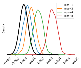
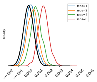
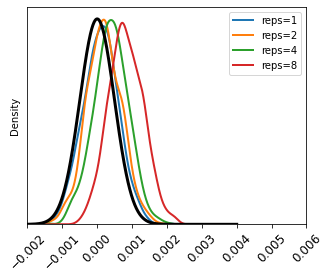
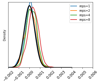
Figure 1: Density plots of cosine values during $\varepsilon$ estimation on StackOverflow. Each plot shows one of the four values of noise in Table 3, and within each plot are the four values of canary repetitions (1, 2, 4, 8). The black curve in each plot is the pdf of the null hypothesis distribution ${\mathcal{N}}(0,1/d)$. In the first plot with no noise ($\varepsilon=\infty$), the distributions are easily separable, with increasing separation for more canary repetitions. At higher levels of noise, distributions are less separable, even with several repetitions.

5.2 Experiments with multiple canary presentations

Here we highlight the ability of our method to estimate privacy when we vary not only the threat model, but also aspects of the training algorithm that may reasonably be expected to change privacy properties, but for which no tight analysis has been obtained. We consider presenting each canary a fixed multiple number of times, modeling the scenario in which clients are only allowed to check in for training every so often. In a real system, a client may not participate in every period, but to obtain worst-case estimates, we present the canary in every period.

In Figure 1 we show kernel density estimation plots of the canary cosine sets. As the number of presentations increases in each plot, the distributions become more and more clearly separated. On the other hand, as the amount of noise increases across the four plots, they all converge to the null hypothesis distribution. Also visible on this figure is that the distributions are roughly Gaussian-shaped, justifying the Gaussian approximation that is used in our estimation method. In Appendix B we give quantitative evidence for this observation. Finally we compare $\varepsilon_{\text{lo}}$ to our $\varepsilon_{\text{est}}$ with multiple canary presentations in Figure 2. For each noise level, $\varepsilon_{\text{est}}$ increases dramatically with increasing presentations, confirming our intuition that seeing examples multiple times dramatically reduces privacy.

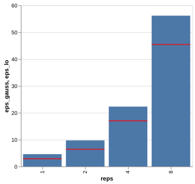
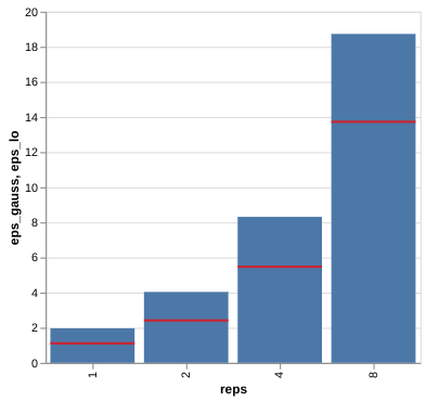
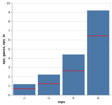
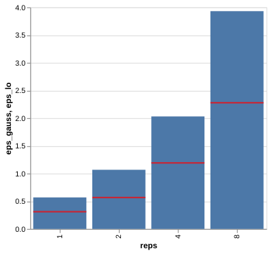
Figure 2: Estimated $\varepsilon$ and lower bound on StackOverflow. The blue bars are our $\varepsilon_{\text{est}}$ and red ticks are the $\varepsilon_{\text{lo}}$ 95%-confidence lower bound for the four values of noise in Table 3 and four values of canary repetitions (1, 2, 4, 8). Note the difference of y-axis scales in each plot. Our estimate of epsilon increases sharply with the number of canary repetitions, confirming that limiting client participation improves privacy.

Noise	analytical $\varepsilon$	$\varepsilon_{\text{lo}}$-all	$\varepsilon_{\text{est}}$-all	$\varepsilon_{\text{lo}}$-final	$\varepsilon_{\text{est}}$-final
0.0	$\infty$	6.25	16300	6.86	8.87
0.0487	300	6.25	258	2.59	3.71
0.0958	100	5.46	76.9	1.34	2.05
0.2207	30	1.42	5.97	0.623	0.992

Table 4: Estimating $\varepsilon$ for EMNIST using all model deltas vs. using the final model only. $\varepsilon_{\text{lo}}$ is the empirical 95% lower bound from our modified Jagielski et al. [2020] method. The high values of $\varepsilon_{\mathrm{est}}$-all indicate that membership inference is easy when the attacker has access to all iterates. On the other hand, when only the final model is observed, $\varepsilon_{\text{est}}$-final is far lower.

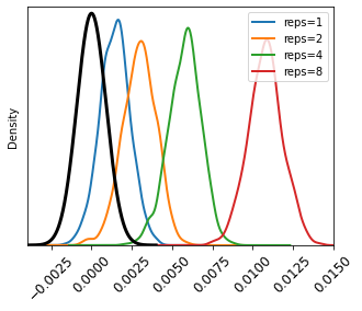
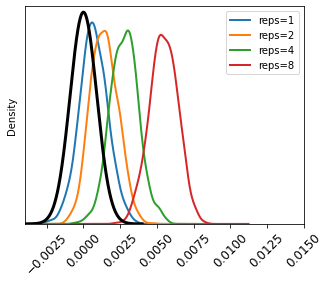
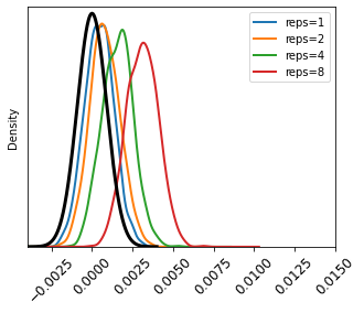
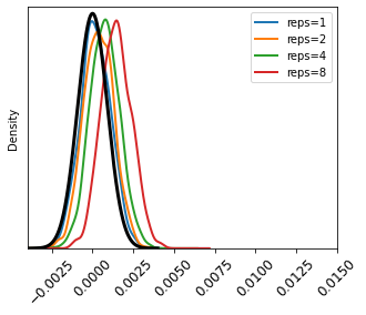
Figure 3: Density plots of cosine values during $\varepsilon$ estimation on EMNIST. Each plot shows one of the four values of noise in Table 4, and within each plot are the four values of canary repetitions (1, 2, 4, 8). The black curve in each plot is the pdf of the null hypothesis distribution ${\mathcal{N}}(0,1/d)$. In the first plot with no noise ($\varepsilon=\infty$), the distributions are easily separable, with increasing separation for more canary repetitions. At higher levels of noise, distributions are less separable, even with several repetitions.

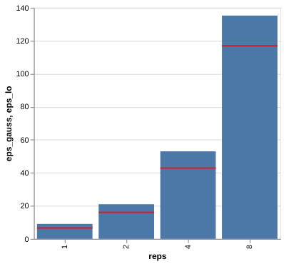
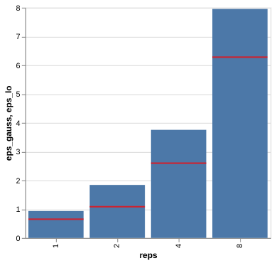
Figure 4: Estimated $\varepsilon$ and lower bound on EMNIST. The blue bars are our $\varepsilon_{\text{est}}$ and red ticks are the $\varepsilon_{\text{lo}}$ 95%-confidence lower bound for the four values of noise in Table 4 and four values of canary repetitions (1, 2, 4, 8). Our estimate of epsilon increases sharply with the number of canary repetitions, confirming that limiting client participation improves privacy.

5.2.1 Results on EMNIST

Here we present similar results on the EMNIST character recognition dataset. It contains 814k characters written by 3383 users. The model is a CNN with 1.2M parameters. The users are shuffled and we train for 15 epochs with 101 clients per round (which amounts to a total of 500 rounds). The optimizers on client and server are both SGD, with learning rates 0.031 and 1.0 respectively, and momentum of 0.9 on the server. The client batch size is 16.

Table 4 shows the empirical epsilon estimates using either all model iterates or only the final model. As with the StackOverflow next word prediction task, using all iterates and a low amount of noise gives us estimates close to the analytical upper bound, while using only the final model gives a much smaller estimate.

Figures 3 and 4 demonstrate the effect of increasing the number of canary repetitions for EMNIST. The results are qualitatively similar to the case of StackOverflow.

5.3 Experiments comparing estimates for single and multiple runs

In the limit of high model dimensionality, canaries are essentially mutually orthogonal, and therefore they will interfere minimally with each other’s cosines to the model. In this section we give evidence that including many canaries in one run does not significantly perturb the estimated epsilon values, for the model dimensionalities explored in our experiments. The ideal comparison would be to train 1000 models, each with one canary, to collect a set of truly independent statistics, and compare our $\varepsilon$ with the $\varepsilon$ estimated from these statistics. However this is computationally infeasible, particularly if we want to perform the entire process multiple times to obtain confidence intervals. Instead, we reduce the number of canaries per run to one hundred and train ten independent models to collect a total of 1000 canary cosine statistics from which to estimate $\varepsilon$. We repeated the experiment 50 times for two different noise multipliers, which still amounts to training a total of 1000 models. (Ten runs, two noise settings, fifty repetitions.)

Noise	runs/canaries	0.1	0.3	0.5	0.7	0.9
0.0496	1/1000	1.59	1.75	1.97	2.15	2.46
0.0496	10/100	1.65	1.80	1.92	2.16	2.32
0.0986	1/1000	0.81	1.06	1.18	1.33	1.54
0.0986	10/100	0.87	1.03	1.16	1.36	1.78

Table 5: Quantiles of $\varepsilon$ over fifty experiments using either one run with 1000 canaries or ten runs with 100 canaries each. For both noise multipliers, the distributions are very close.

The results on the StackOverflow dataset with the same setup as in Section 5 are shown in Table 5. We report the 0.1, 0.3, 0.5, 0.7 and 0.9 quantiles of the distribution of $\varepsilon$ over 50 experiments. For both noise multipliers, the distributions of privacy parameter estimates are quite close. Interestingly, our epsilon estimates do not vary significantly even as the number of canaries per run varies by an order of magnitude. This finding provides evidence that our one-shot empirical estimation method (using multiple canaries in one training run) provides similar epsilon estimates as using multiple training runs to obtain independent estimates (as done by most prior work in privacy auditing). The main advantage of our method is its ability to estimate privacy in a single training run, resulting in increased computational efficiency compared to previous methods.

5.4 Empirical comparison with CANIFE

As discussed in Section 2, our method is significantly more general than the CANIFE method of Maddock et al. [2022]. CANIFE periodically audits individual rounds to get a per-round $\hat{\varepsilon}_{r}$, estimates the noise for the round $\hat{\sigma}_{r}$ by inverting the computation of $\varepsilon$ for the Gaussian mechanism, and uses standard composition theorems to determine a final cumulative epsilon. Therefore the estimate will be inaccurate if the assumptions of those composition theorems do not strictly hold, for example, if clients are not sampled uniformly and independently at each round, or the noise is not in fact isotropic Gaussian, and independent across rounds. In contrast, our method will detect if any unanticipated aspect of training causes some canaries to have more influence on the final model in terms of higher canary/model dot product, leading in turn to higher $\varepsilon$ estimates. Also the CANIFE method of crafting canaries is model/dataset specific and computationally expensive, whereas ours is model/dataset agnostic and adds negligible computation.

It is still interesting to see how the methods compare in the limited setting where CANIFE’s assumptions do hold. We trained a two-layer feedforward network on the fashion MNIST dataset. Following experiments in Maddock et al. [2022], we used a canary design pool size of 512, took 2500 canary optimization steps to find a canary example optimizing pixels and soft label, ran auditing every 100 rounds with 100 attack scores on each auditing round. We trained with a clip norm of 1.0 and noise multiplier of 0.2 for one epoch with a batch size of 128, which corresponds to an analytical $\varepsilon$ of 34.5.

CANIFE output an $\varepsilon$ estimate of mean $0.879$ and standard deviation $0.124$. Our method (using 1000 seen and 1000 unseen model canaries) estimated $\varepsilon$ with a mean of $6.76$ and std of $1.06$, much closer to the analytical bound.

6 Conclusion

In this work we have introduced a novel method for empirically estimating the privacy loss during federated training of a model with DP-FedAvg. For natural production-sized problems (millions of parameters, hundreds of thousands of clients), it produces reasonable privacy estimates during the same single training run used to train model parameters, without significantly degrading the utility of the model, and does not require any prior knowledge of the task, data, or model. The resulting $\varepsilon_{\text{est}}$ can be interpreted as bounding the degree of confidence that a particular strong adversary could have in performing membership inference. It gives a reasonable metric for comparing how privacy loss changes between arbitrary variants of client-participation, or other variations of DP-FedAvg for which no method for producing a tight analytical estimate of $\varepsilon$ is known.

In future work we would like to explore how our metric is related to formal bounds on the privacy loss. We would also like to open the door to empirical refutation of our epsilon metric – that is, for researchers to attempt to design a successful attack on a training mechanism for which our metric nevertheless estimates a low value of epsilon. To the extent that we are confident no such attack exists, we can be assured that our estimate is faithful. We note that this is the case with techniques like the cryptographic hash function SHA-3: although no proof exists that inverting SHA-3 is computationally difficult, it is used in high-security applications because highly motivated security experts have not been able to mount a successful inversion attack in the 11 years of its existence.

Appendix A Proofs of theorems from the main text

See 3.1

Proof.

Without loss of generality, we can take $v$ to be constant. First we describe the distribution of the angle $\theta\in[0,\pi]$ between $s$ and $v$, then change variables to get the distribution of its cosine $\tau$. Consider the spherical cap of points on the $d$-sphere with angle to $v$ less or equal to $\theta$, having $(d\!-\!1)$-measure $A_{d}(\theta)$. The boundary of $A_{d}(\theta)$ is a $(d\!-\!1)$-sphere with radius $\sin\theta$ and $(d\!-\!2)$-measure $M_{d}(\theta)=S_{d-1}\sin^{d-2}\theta$, where $S_{d}=2\pi^{\frac{d}{2}}/\Gamma(\frac{d}{2})$ is the surface area of the unit $d$-sphere. (For example, the boundary of the 3-d spherical cap with maximum angle $\theta$ is a circle (2-sphere) with radius $\sin\theta$ and circumference $2\pi\sin(\theta)$.) Normalizing by the total area of the sphere $S_{d}$, the density of the angle is

$$\phi_{d}(\theta) =S_{d}^{-1}\frac{d}{d\theta}A_{d}(\theta)$$

$$=\left(\frac{2\pi^{\frac{d}{2}}}{\Gamma(\frac{d}{2})}\right)^{-1}\left(\frac{2\pi^{\frac{d-1}{2}}}{\Gamma(\frac{d-1}{2})}\right)\sin^{d-2}\theta$$

$$=\frac{\Gamma(\frac{d}{2})}{\Gamma(\frac{d-1}{2})\sqrt{\pi}}\sin^{d-2}\theta.$$

Now change variables to express it in terms of the angle cosine $\tau=\cos(\theta)\in[-1,1]$:

$$f_{d}(\tau) =\phi_{d}(\arccos\tau)\cdot\left|\frac{d}{d\tau}\arccos(\tau)\right|$$

$$=\frac{\Gamma(\frac{d}{2})}{\Gamma(\frac{d-1}{2})\sqrt{\pi}}\bigl{[}\sin(\arccos\tau)\bigr{]}^{d-2}\left|-\frac{1}{\sqrt{1-\tau^{2}}}\right|$$

$$=\frac{\Gamma(\frac{d}{2})}{\Gamma(\frac{d-1}{2})\sqrt{\pi}}\frac{\left(\sqrt{1-\tau^{2}}\right)^{d-2}}{\sqrt{1-\tau^{2}}}$$

$$=\frac{\Gamma(\frac{d}{2})}{\Gamma(\frac{d-1}{2})\sqrt{\pi}}(1-\tau^{2})^{\frac{d-3}{2}}.$$

∎

See 3.2

Proof.

The distribution function of $t\in[-\sqrt{d},\sqrt{d}]$ is

$$\hat{f}_{d}(t) =\frac{1}{\sqrt{d}}\frac{\Gamma(\frac{d}{2})}{\Gamma(\frac{d-1}{2})\sqrt{\pi}}\left(1-(t/\sqrt{d})^{2}\right)^{\frac{d-3}{2}}$$

$$=\frac{\Gamma(\frac{d}{2})}{\Gamma(\frac{d-1}{2})\sqrt{\pi d}}\left(1-t^{2}/d\right)^{\frac{d-3}{2}}.$$

Taking the limit:

$$\lim_{d\rightarrow\infty}\hat{f}_{d}(t) =\biggl{(}\lim_{d\rightarrow\infty}\frac{\Gamma(\frac{d}{2})}{\Gamma(\frac{d-1}{2})\sqrt{\pi d}}\biggr{)}\cdot\biggl{(}\lim_{d\rightarrow\infty}\left(1-t^{2}/d\right)^{\frac{d}{2}}\biggr{)}\cdot\biggl{(}\lim_{d\rightarrow\infty}\left(1-t^{2}/d\right)^{-\frac{3}{2}}\biggr{)}$$

$$=\frac{1}{\sqrt{2\pi}}\cdot e^{-t^{2}/2}\cdot 1,$$

where we have used the fact that $\frac{\Gamma(\frac{d}{2})}{\Gamma(\frac{d-1}{2})}\sim\sqrt{d/2}$.

∎

Lemma A.1.

If $\tau$ is distributed according to the cosine angle distribution described in Theorem 3.1, then $\text{Var}\!\left[\tau\right]=1/d$.

Proof.

Let $x=(x_{1},\dots,x_{d})$ be uniform on the unit $d$-sphere. Then $x_{1}=\langle x,e_{1}\rangle$ has the required distribution, where $e_{1}$ is the first standard basis vector. $\mathbb{E}\!\left[x_{1}\right]$ is zero, so we are interested in $\text{Var}\!\left[x_{1}\right]=\mathbb{E}\!\left[x_{1}^{2}\right]$. Since $\sum_{i}x_{i}^{2}=1$, we have that $\mathbb{E}\!\left[\sum_{i}x_{i}^{2}\right]=\sum_{i}\mathbb{E}\!\left[x_{i}^{2}\right]=1$. But all of the $x_{i}$ have the same distribution, so $\mathbb{E}\!\left[x_{1}^{2}\right]=1/d$. ∎

See 3.3

Proof.

Rewrite

$$\sqrt{d}\hat{\mu} =\sqrt{d}\left(\frac{1}{k}\sum_{i}\frac{\langle c_{i},\rho\rangle}{||\rho||}\right)$$

$$=\left(\frac{||\rho||}{\sqrt{d}}\right)^{-1}\left(\frac{1}{k}\sum_{i}\langle c_{i},\rho\rangle\right).$$

We will show that $\frac{||\rho||^{2}}{d}\overset{p}{\longrightarrow}\sigma^{2}$, while $\frac{1}{k}\sum_{i}\langle c_{i},\rho\rangle\overset{p}{\longrightarrow}1$.

Note that $||Z||^{2}$ is Chi-squared distributed with mean $d$ and variance $2d$. Also, for all $i\neq j$, $\langle c_{i},c_{j}\rangle$ is distributed according to the cosine distribution discussed in Theorem 3.1 and Lemma A.1 with mean 0 and variance $1/d$. Therefore,

$$\mathbb{E}\!\left[\frac{||\rho||^{2}}{d}\right] =\frac{1}{d}\left\langle\sum_{i}c_{i}+\sigma Z,\ \sum_{i}c_{i}+\sigma Z\right\rangle$$

$$=\frac{1}{d}\left(\sum_{i,j}\mathbb{E}\!\left[\langle c_{i},c_{j}\rangle\right]+2\sigma\sum_{i}\mathbb{E}\!\left[\langle Z,c_{i}\rangle\right]+\sigma^{2}\mathbb{E}\!\left[||Z||^{2}\right]\right)$$

$$=\frac{1}{d}\left(k+\sigma^{2}d\right)$$

$$=\sigma^{2}+o(1).$$

Next, note that all of the following dot products are pairwise uncorrelated: $\langle Z,Z\rangle$, $\langle Z,c_{i}\rangle$ (for all $i$), and $\langle c_{i},c_{j}\rangle$ (for all $i,j$). Therefore the variance decomposes:

$$\text{Var}\!\left[\frac{||\rho||^{2}}{d}\right] =\frac{1}{d^{2}}\left(\sum_{i,j}\text{Var}\!\left[\langle c_{i},c_{j}\rangle\right]+2\sigma^{2}\sum_{i}\text{Var}\!\left[\langle Z,c_{i}\rangle\right]+\sigma^{4}\text{Var}\!\left[||Z||^{2}\right]\right)$$

$$=\frac{1}{d^{2}}\left(\frac{k(k-1)}{d}+2k\sigma^{2}+2\sigma^{4}d\right),$$

$$=O(d^{-1}).$$

Taken together, these imply that $\frac{||\rho||}{\sqrt{d}}\overset{p}{\longrightarrow}\sigma$.

Now reusing many of the same calculations,

$$\mathbb{E}\!\left[\frac{1}{k}\sum_{i}\langle c_{i},\rho\rangle\right]=\frac{1}{k}\left(k+\sum_{i\neq j}\mathbb{E}\!\left[\langle c_{i},c_{j}\rangle\right]+\sigma\sum_{i}\mathbb{E}\!\left[\langle Z,c_{i}\rangle\right]\right)=1,$$

and

$$\text{Var}\!\left[\frac{1}{k}\sum_{i}\langle c_{i},\rho\rangle\right] =\frac{1}{k^{2}}\left(\sum_{i\neq j}\text{Var}\!\left[\langle c_{i},c_{j}\rangle\right]+\sigma^{2}\sum_{i}\text{Var}\!\left[\langle Z,c_{i}\rangle\right]\right)$$

$$=\frac{1}{k^{2}}\left(\frac{k(k-1)}{d}+k\sigma^{2}\right)$$

$$=o(1),$$

which together imply that $\frac{1}{k}\sum_{i}\langle c_{i},\rho\rangle\overset{p}{\longrightarrow}1$.

Now consider

$$d\hat{\sigma}^{2} =d\left(\frac{1}{k}\sum_{i}g_{i}^{2}-\biggl{(}\frac{1}{k}\sum_{i}g_{i}\biggr{)}^{2}\right)$$

$$=\frac{d}{||\rho||^{2}}\left(\frac{1}{k}\sum_{i}\langle c_{i},\rho\rangle^{2}-\left(\frac{1}{k}\sum_{i}\langle c_{i},\rho\rangle\right)^{2}\right).$$

We already have that $\frac{d}{||\rho||^{2}}\overset{p}{\longrightarrow}\frac{1}{\sigma^{2}}$ and $\frac{1}{k}\sum_{i}\langle c_{i},\rho\rangle\overset{p}{\longrightarrow}1$, so it will be sufficient to show $\frac{1}{k}\sum_{i}\langle c_{i},\rho\rangle^{2}\overset{p}{\longrightarrow}1+\sigma^{2}$. Again using the uncorrelatedness of all pairs of dot products under consideration,

$$\mathbb{E}\!\left[\frac{1}{k}\sum_{i}\langle c_{i},\rho\rangle^{2}\right] =\frac{1}{k}\sum_{i}\mathbb{E}\!\left[\left(\sum_{j}\langle c_{i},c_{j}\rangle+\langle c_{i},\sigma Z\rangle\right)^{2}\right]$$

$$=\frac{1}{k}\sum_{i}\left(\sum_{j,\ell}\mathbb{E}\!\left[\langle c_{i},c_{j}\rangle\langle c_{i},c_{\ell}\rangle\right]+2\sum_{j}\mathbb{E}\!\left[\langle c_{i},c_{j}\rangle\langle c_{i},\sigma Z\rangle\right]+\mathbb{E}\!\left[\langle c_{i},\sigma Z\rangle^{2}\right]\right)$$

$$=\frac{1}{k}\sum_{i}\left(\sum_{j,\ell}\mathbb{I}\{j=i,\ell=i\}+0+\sigma^{2}\right)$$

$$=1+\sigma^{2}.$$

Also,

$$\text{Var}\!\left[\frac{1}{k}\sum_{i}\langle c_{i},\rho\rangle^{2}\right] =\frac{1}{k^{2}}\sum_{i}\left(\sum_{j,\ell}\text{Var}\!\left[\langle c_{i},c_{j}\rangle\langle c_{i},c_{\ell}\rangle\right]+2\sum_{j}\text{Var}\!\left[\langle c_{i},c_{j}\rangle\langle c_{i},\sigma Z\rangle\right]+\text{Var}\!\left[\langle c_{i},\sigma Z\rangle^{2}\right]\right).$$

We’ll bound each of these terms to show the sum is $o(1)$.

First, look at $\text{Var}\!\left[\langle c_{i},c_{j}\rangle\langle c_{i},c_{\ell}\rangle\right]$. If $i=j=\ell$, it is 0. If $j\neq\ell$,

$$\text{Var}\!\left[\langle c_{i},c_{j}\rangle\langle c_{i},c_{\ell}\rangle\right] =\mathbb{E}\!\left[\langle c_{i},c_{j}\rangle^{2}\langle c_{i},c_{\ell}\rangle^{2}\right]-\mathbb{E}\!\left[\langle c_{i},c_{j}\rangle\langle c_{i},c_{\ell}\rangle\right]^{2}$$

$$=\mathbb{E}\!\left[\mathbb{E}\!\left[\langle c_{i},c_{j}\rangle^{2}\langle c_{i},c_{\ell}\rangle^{2}\mid c_{i}\right]\right]$$

$$=\mathbb{E}\!\left[\mathbb{E}\!\left[\langle c_{i},c_{j}\rangle^{2}\mid c_{i}\right]\mathbb{E}\!\left[\langle c_{i},c_{\ell}\rangle^{2}\mid c_{i}\right]\right]$$

$$=\begin{cases}1/d&\text{$j=i$ or $\ell=i$,}\\ 1/d^{2}&\text{$j\neq i$ and $\ell\neq i$,}\end{cases}$$

and if $j=\ell\neq i$,

$$\text{Var}\!\left[\langle c_{i},c_{j}\rangle\langle c_{i},c_{\ell}\rangle\right] =\text{Var}\!\left[\langle c_{i},c_{j}\rangle^{2}\right]$$

$$=\mathbb{E}\!\left[\langle c_{i},c_{j}\rangle^{4}\right]-\mathbb{E}\!\left[\langle c_{i},c_{j}\rangle^{2}\right]^{2}$$

$$\leq\mathbb{E}\!\left[\langle c_{i},c_{j}\rangle^{4}\right]$$

$$\leq\mathbb{E}\!\left[\langle c_{i},c_{j}\rangle^{2}\right]$$

$$=1/d.$$

Together we have

$$\frac{1}{k^{2}}\sum_{i,j,\ell}\text{Var}\!\left[\langle c_{i},c_{j}\rangle\langle c_{i},c_{\ell}\rangle\right]\leq\frac{1}{k^{2}}\left(\frac{2k(k-1)}{d}+\frac{k(k-1)(k-2)}{d^{2}}+\frac{k(k-1)}{d}\right)=O(d^{-1}).$$

Now for $\text{Var}\!\left[\langle c_{i},c_{j}\rangle\langle c_{i},\sigma Z\rangle\right]$. If $i=j$, then it is $\sigma^{2}.$ If $i\neq j$,

$$\text{Var}\!\left[\langle c_{i},c_{j}\rangle\langle c_{i},\sigma Z\rangle\right] =\mathbb{E}\!\left[\langle c_{i},c_{j}\rangle^{2}\langle c_{i},\sigma Z\rangle^{2}\right]-\mathbb{E}\!\left[\langle c_{i},c_{j}\rangle\langle c_{i},\sigma Z\rangle\right]^{2}$$

$$=\mathbb{E}\!\left[\mathbb{E}\!\left[\langle c_{i},c_{j}\rangle^{2}|c_{i}\right]\mathbb{E}\!\left[\langle c_{i},\sigma Z\rangle^{2}|c_{i}\right]\right]$$

$$=\sigma^{2}/d.$$

So,

$$\frac{2}{k^{2}}\sum_{i,j}\text{Var}\!\left[\langle c_{i},c_{j}\rangle\langle c_{i},\sigma Z\rangle\right]=\frac{2}{k^{2}}\left(k\sigma^{2}+\frac{k(k-1)\sigma^{2}}{d}\right)=o(1).$$

Finally, $\langle c_{i},Z\rangle^{2}$ is Chi-squared distributed with one degree of freedom, so $\text{Var}\!\left[\langle c_{i},\sigma Z\rangle^{2}\right]=2\sigma^{4}$, and

$$\frac{1}{k^{2}}\sum_{i}\text{Var}\!\left[\langle c_{i},\sigma Z\rangle^{2}\right]=\frac{2\sigma^{4}}{k}=o(1).$$

∎

Noise	1 rep	2 reps	4 reps	8 reps
0	0.219	0.225	0.336	0.366
0.0496	0.462	0.242	0.444	0.576
0.0986	0.224	0.369	0.295	0.445
0.2317	1.23	0.636	0.523	0.255

Table 6: Anderson statistics for each set of canary-cosine samples whose densities are shown in Figure 1. For 1000 samples, the Anderson test rejects at 10% significance if the statistic is greater than 0.656, and rejects at 1% significance for value greater than 1.092.

Appendix B Gaussianity of cosine statistics

To our knowledge, there is no way of confidently inferring that a set of samples comes from a given distribution, or even that they come from a distribution that is close to the given distribution in some metric. To quantify the error of our approximation of the cosine statistics with a Gaussian distribution, we apply the Anderson test to each set of cosines in Table 6. It gives us some confidence to see that a strong goodness-of-fit test cannot rule out that the distributions are Gaussian. This is a more quantitative claim than visually comparing a histogram or empirical CDF, as is commonly done.

References

- Abadi et al. [2016] M. Abadi, A. Chu, I. Goodfellow, H. B. McMahan, I. Mironov, K. Talwar, and L. Zhang. Deep learning with differential privacy. In Proceedings of the 2016 ACM SIGSAC conference on computer and communications security, pages 308–318, 2016.
- Andrew et al. [2021] G. Andrew, O. Thakkar, B. McMahan, and S. Ramaswamy. Differentially private learning with adaptive clipping. Advances in Neural Information Processing Systems, 34:17455–17466, 2021.
- Balle and Wang [2018] B. Balle and Y.-X. Wang. Improving the gaussian mechanism for differential privacy: Analytical calibration and optimal denoising. In International Conference on Machine Learning, pages 394–403. PMLR, 2018.
- Balle et al. [2022] B. Balle, G. Cherubin, and J. Hayes. Reconstructing training data with informed adversaries. In 2022 IEEE Symposium on Security and Privacy (SP), pages 1138–1156. IEEE, 2022.
- Bell et al. [2020] J. H. Bell, K. A. Bonawitz, A. Gascón, T. Lepoint, and M. Raykova. Secure single-server aggregation with (poly) logarithmic overhead. In Proceedings of the 2020 ACM SIGSAC Conference on Computer and Communications Security, pages 1253–1269, 2020.
- Bonawitz et al. [2017] K. Bonawitz, V. Ivanov, B. Kreuter, A. Marcedone, H. B. McMahan, S. Patel, D. Ramage, A. Segal, and K. Seth. Practical secure aggregation for privacy-preserving machine learning. In proceedings of the 2017 ACM SIGSAC Conference on Computer and Communications Security, pages 1175–1191, 2017.
- Bonawitz et al. [2022] K. Bonawitz, P. Kairouz, B. Mcmahan, and D. Ramage. Federated learning and privacy. Commun. ACM, 65(4):90–97, mar 2022. ISSN 0001-0782. doi: 10.1145/3500240. URL https://doi.org/10.1145/3500240.
- Carlini et al. [2021] N. Carlini, F. Tramer, E. Wallace, M. Jagielski, A. Herbert-Voss, K. Lee, A. Roberts, T. Brown, D. Song, U. Erlingsson, A. Oprea, and C. Raffel. Extracting training data from large language models. In 30th USENIX Security Symposium (USENIX Security 2021), 2021.
- Carlini et al. [2022] N. Carlini, S. Chien, M. Nasr, S. Song, A. Terzis, and F. Tramer. Membership inference attacks from first principles. In IEEE Symposium on Security and Privacy (SP), pages 1519–1519, Los Alamitos, CA, USA, May 2022. IEEE Computer Society. doi: 10.1109/SP46214.2022.00090. URL https://doi.ieeecomputersociety.org/10.1109/SP46214.2022.00090.
- Choquette-Choo et al. [2022] C. A. Choquette-Choo, H. B. McMahan, K. Rush, and A. Thakurta. Multi-epoch matrix factorization mechanisms for private machine learning. arXiv preprint arXiv:2211.06530, 2022.
- Denissov et al. [2022] S. Denissov, H. B. McMahan, J. K. Rush, A. Smith, and A. G. Thakurta. Improved differential privacy for SGD via optimal private linear operators on adaptive streams. In A. H. Oh, A. Agarwal, D. Belgrave, and K. Cho, editors, Advances in Neural Information Processing Systems, 2022. URL https://openreview.net/forum?id=i9XrHJoyLqJ.
- Desfontaines [2018] D. Desfontaines. Differential privacy in (a bit) more detail. https://desfontain.es/privacy/differential-privacy-in-more-detail.html, 2018. Accessed 2023-09-28.
- Ding et al. [2018] Z. Ding, Y. Wang, G. Wang, D. Zhang, and D. Kifer. Detecting violations of differential privacy. In Proceedings of the 2018 ACM SIGSAC Conference on Computer and Communications Security, pages 475–489, 2018.
- Dwork and Roth [2014] C. Dwork and A. Roth. The algorithmic foundations of differential privacy. Foundations and Trends® in Theoretical Computer Science, 9(3–4):211–407, 2014. ISSN 1551-305X. doi: 10.1561/0400000042. URL http://dx.doi.org/10.1561/0400000042.
- Dwork et al. [2006] C. Dwork, F. McSherry, K. Nissim, and A. Smith. Calibrating noise to sensitivity in private data analysis. In Conference on Theory of Cryptography, TCC ’06, pages 265–284, New York, NY, USA, 2006.
- Feldman et al. [2021] V. Feldman, A. McMillan, and K. Talwar. A simple and nearly optimal analysis of privacy amplification by shuffling. In FOCS, 2021. URL https://arxiv.org/pdf/2012.12803.pdf.
- Feldman et al. [2023] V. Feldman, A. McMillan, and K. Talwar. Stronger privacy amplification by shuffling for rényi and approximate differential privacy. In Proceedings of the 2023 Annual ACM-SIAM Symposium on Discrete Algorithms (SODA), pages 4966–4981. SIAM, 2023.
- Gilbert and McMillan [2018] A. C. Gilbert and A. McMillan. Property Testing for Differential Privacy. In 2018 56th Annual Allerton Conference on Communication, Control, and Computing (Allerton), pages 249–258. IEEE, 2018.
- Haim et al. [2022] N. Haim, G. Vardi, G. Yehudai, michal Irani, and O. Shamir. Reconstructing training data from trained neural networks. In A. H. Oh, A. Agarwal, D. Belgrave, and K. Cho, editors, Advances in Neural Information Processing Systems, 2022. URL https://openreview.net/forum?id=Sxk8Bse3RKO.
- Jagielski et al. [2020] M. Jagielski, J. Ullman, and A. Oprea. Auditing differentially private machine learning: How private is private sgd? In Proceedings of the 34th International Conference on Neural Information Processing Systems, NIPS’20, Red Hook, NY, USA, 2020. Curran Associates Inc. ISBN 9781713829546.
- Jagielski et al. [2023] M. Jagielski, S. Wu, A. Oprea, J. Ullman, and R. Geambasu. How to combine membership-inference attacks on multiple updated machine learning models. Proceedings on Privacy Enhancing Technologies, 3:211–232, 2023.
- Kairouz et al. [2015] P. Kairouz, S. Oh, and P. Viswanath. The composition theorem for differential privacy. In F. Bach and D. Blei, editors, Proceedings of the 32nd International Conference on Machine Learning, volume 37 of Proceedings of Machine Learning Research, pages 1376–1385, Lille, France, 07–09 Jul 2015. PMLR. URL https://proceedings.mlr.press/v37/kairouz15.html.
- Kairouz et al. [2021a] P. Kairouz, B. McMahan, S. Song, O. Thakkar, A. Thakurta, and Z. Xu. Practical and private (deep) learning without sampling or shuffling. In International Conference on Machine Learning, pages 5213–5225. PMLR, 2021a.
- Kairouz et al. [2021b] P. Kairouz, H. B. McMahan, B. Avent, A. Bellet, M. Bennis, A. N. Bhagoji, K. Bonawitz, Z. Charles, G. Cormode, R. Cummings, et al. Advances and open problems in federated learning. Foundations and Trends® in Machine Learning, 14(1–2):1–210, 2021b.
- Liu and Oh [2019] X. Liu and S. Oh. Minimax Optimal Estimation of Approximate Differential Privacy on Neighboring Databases. In Advances in Neural Information Processing Systems, volume 32, 2019.
- Lu et al. [2022] F. Lu, J. Munoz, M. Fuchs, T. LeBlond, E. V. Zaresky-Williams, E. Raff, F. Ferraro, and B. Testa. A general framework for auditing differentially private machine learning. In A. H. Oh, A. Agarwal, D. Belgrave, and K. Cho, editors, Advances in Neural Information Processing Systems, 2022. URL https://openreview.net/forum?id=AKM3C3tsSx3.
- Maddock et al. [2022] S. Maddock, A. Sablayrolles, and P. Stock. Canife: Crafting canaries for empirical privacy measurement in federated learning, 2022. URL https://arxiv.org/abs/2210.02912.
- McMahan et al. [2017] B. McMahan, E. Moore, D. Ramage, S. Hampson, and B. A. y. Arcas. Communication-Efficient Learning of Deep Networks from Decentralized Data. In A. Singh and J. Zhu, editors, Proceedings of the 20th International Conference on Artificial Intelligence and Statistics, volume 54 of Proceedings of Machine Learning Research, pages 1273–1282. PMLR, 20–22 Apr 2017. URL https://proceedings.mlr.press/v54/mcmahan17a.html.
- McMahan et al. [2018] H. B. McMahan, D. Ramage, K. Talwar, and L. Zhang. Learning differentially private recurrent language models. In International Conference on Learning Representations, 2018.
- Mo et al. [2021] F. Mo, H. Haddadi, K. Katevas, E. Marin, D. Perino, and N. Kourtellis. Ppfl: privacy-preserving federated learning with trusted execution environments. In Proceedings of the 19th annual international conference on mobile systems, applications, and services, pages 94–108, 2021.
- Nasr et al. [2021] M. Nasr, S. Songi, A. Thakurta, N. Papemoti, and N. Carlin. Adversary instantiation: Lower bounds for differentially private machine learning. In 2021 IEEE Symposium on Security and Privacy (SP), pages 866–882. IEEE, 2021.
- Nasr et al. [2023] M. Nasr, J. Hayes, T. Steinke, B. Balle, F. Tramèr, M. Jagielski, N. Carlini, and A. Terzis. Tight auditing of differentially private machine learning. arXiv preprint arXiv:2302.07956, 2023.
- Pillutla et al. [2023] K. Pillutla, G. Andrew, P. Kairouz, H. B. McMahan, A. Oprea, and S. Oh. Unleashing the power of randomization in auditing differentially private ml. arXiv preprint arXiv:2305.18447, 2023.
- Reddi et al. [2020] S. Reddi, Z. Charles, M. Zaheer, Z. Garrett, K. Rush, J. Konečnỳ, S. Kumar, and H. B. McMahan. Adaptive federated optimization. arXiv preprint arXiv:2003.00295, 2020.
- Shokri et al. [2017] R. Shokri, M. Stronati, C. Song, and V. Shmatikov. Membership inference attacks against machine learning models. In 2017 IEEE Symposium on Security and Privacy (SP), pages 3–18. IEEE, 2017.
- Steinke [2022] T. Steinke. Composition of differential privacy & privacy amplification by subsampling, 2022.
- Steinke et al. [2023] T. Steinke, M. Nasr, and M. Jagielski. Privacy auditing with one (1) training run. arXiv preprint arXiv:2305.08846, 2023.
- Yeom et al. [2018] S. Yeom, I. Giacomelli, M. Fredrikson, and S. Jha. Privacy risk in machine learning: Analyzing the connection to overfitting. In 2018 IEEE 31st Computer Security Foundations Symposium (CSF), pages 268–282. IEEE, 2018.