Statistical methods for partitioning ribbon and globally-distributed flux using data from the Interstellar Boundary Explorer

Abstract

NASA’s Interstellar Boundary Explorer (IBEX) satellite collects data on energetic neutral atoms (ENAs) that can provide insight into the heliosphere boundary between our solar system and interstellar space. Using these data, scientists can construct maps of the ENA intensities (often, expressed in terms of flux) observed in all directions. The ENA flux observed in these maps is believed to come from at least two distinct sources: one source which manifests as a ribbon of concentrated ENA flux and one source (or possibly several) that manifest as smoothly-varying globally-distributed flux. Each ENA source type and its corresponding ENA intensity map is of separate scientific interest.
In this paper, we develop statistical methods for separating the total ENA intensity maps into two source-specific maps (ribbon and globally-distributed flux) and estimating corresponding uncertainty. Key advantages of the proposed method include enhanced model flexibility and improved propagation of estimation uncertainty. We evaluate the proposed methods on simulated data designed to mimic realistic data settings. We also propose new methods for estimating the center of the near-elliptical ribbon in the sky, which can be used in the future to study the location and variation of the local interstellar magnetic field.

1 Introduction

The Interstellar Boundary Explorer (IBEX) satellite collects data on energetic neutral atoms as part of a U.S. National Aeronautics and Space Administration (NASA) mission to better understand the boundary of our solar system (Funsten et al., 2009a). Energetic neutral atoms (ENAs) are fast-moving particles with net zero charge and are believed to largely originate from interactions occuring at the heliospheric boundary between our solar system and interstellar space. Using these data, scientists can construct a pixelated map of estimated ENA intensities/rates (often, expressed in terms of flux) observed in all directions along with corresponding uncertainties, which can provide greater insight into the heliospheric boundary (Funsten et al., 2009b).
The ENA flux observed in these maps is believed to come from (at least) two distinct sources: the globally-distributed flux (GDF; believed to be primarily generated in the inner heliosheath) and a second source (attributed to charge exchange between secondary pick-up ions and interstellar neutral atoms in the outer heliosheath) resulting in a ribbon of concentrated ENA intensity (McComas et al., 2009; Schwadron et al., 2014; Zirnstein et al., 2015). The physics behind the formation of the ENA ribbon are not fully understood, and there are several competing hypotheses (McComas et al., 2014). Both sources of ENAs and their corresponding flux maps are each of scientific interest, and an intermediate scientific objective is to accurately partition the ENA map into GDF- and ribbon-specific maps, which can be used for downstream study of heliosphere temporal dynamics and plasma interactions. The problem of partitioning the ENA rate map is very challenging; the map separation is not identified by the data alone and must be strongly informed by assumptions. However, these assumptions must be general enough and implemented with finesse to avoid obscuring real physical phenomena and introducing bias in downstream analyses.
Several authors have proposed strategies for partitioning ENA rate or flux maps, leveraging features of the ribbon morphology. For example, the ribbon appears to be approximately circular (perhaps slightly elliptical) in 3-dimensional space; when the map is viewed from a particular rotational frame and plotted as a latitude/longitude rectangle, the ribbon manifests as a horizontal stripe of concentrated ENA emission (Funsten et al., 2013). Schwadron et al. (2011), Dayeh et al. (2019), and Reisenfeld et al. (2021) use this rotational frame to facilitate ribbon separation, where parametric modeling of the height and shape of this horizontal ribbon within individual longitude slices is used to obtain the map partitioning. Funsten et al. (2013) takes this approach a step further by borrowing information about the ribbon shape, intensity, and location across longitudes.
These existing ribbon separation approaches have several limitations. Firstly, a common assumption is that ribbon cross-sections mirror a Gaussian density within each longitude slice. This assumption is restrictive. For example, one of the popular theories of ribbon generation is associated with a skewed ribbon with a distinctive non-Gaussian shape (Zirnstein et al., 2019a). The ideal map partitioning algorithm should be flexible enough to capture these scientifically-relevant features, facilitating discrimination between competing scientific theories downstream. Secondly, uncertainty in the separated ENA rate maps should be a function of the uncertainty of the total (ribbon + GDF) ENA map and uncertainty due to the separation itself. None of these existing methods account for this latter source of map uncertainty. Recently, Swaczyna et al. (2022) proposed a ribbon separation method based on spherical harmonic decompositions that appears to address these two limitations. However, this approach tends to introduce rippling artifacts into the separated maps and does not leverage any spatial structure present in the ribbon region for GDF map estimation. Additionally, all of the existing ribbon separation methods were developed and tested using 6-degree resolution observed data alone; none of the existing ribbon separation methods have been validated using simulated maps, directly evaluated against other existing methods, or tested on real data maps with higher than 6-degree resolution (Osthus et al., 2022).
In this paper, we propose a flexible statistical method for separating the total ENA rate maps into source-specific maps and for estimating corresponding uncertainty. Through a rigorous validation of these methods in simulated maps and against a competing approach in the literature, we demonstrate that the proposed methods perform well in settings likely encountered in real IBEX data. We also highlight the performance of the proposed methods in real IBEX data maps; a detailed presentation of these real data results will be provided in a follow-up manuscript. Auxiliary to the goal of ribbon separation, we also propose new methods for estimating the center of the near-elliptical ribbon in the sky, which can be used in the future to provide insight into the location and variation of the local interstellar magnetic field (Zirnstein et al., 2016). Together, these methods represent a substantial advancement in the processing of IBEX data and illustrate the value of close collaboration between statisticians and scientific domain experts.

2 Methods

IBEX “maps” are pixelated representations of the intensity of ENAs observable from the IBEX satellite in all directions (e.g., Funsten et al. (2009b)). Estimated maps are generated through a map-making pipeline that converts data on encounters with ENAs into an estimated ENA rate and corresponding uncertainty estimate for each of many spatial latitude/longitude bins of the 3-dimensional sky. Traditionally, IBEX data maps have been generated at a 6-degree resolution using simple method-of-moments estimators and ad hoc spatial smoothing. Recently, Osthus et al. (2022) developed a higher-resolution and statistically rigorous map-making method involving spatial modeling of the ENA rate data and deconvolution to address instrument-related spatial blurring. The methods proposed in our current paper can by applied to either type of input map; we will demonstrate our methods using 2-degree maps generated by Osthus et al. (2022). Through the map-making process, we produce a vector $\mathcal{D}$ of length $J\times K$ representing the estimated ENA rate for each of $J$ longitude bins and $K$ latitude bins of the sky along with an estimated $J\times K$ vector containing the corresponding uncertainty estimates, $\sigma_{D}^{2}$.
The ENAs represented by $\mathcal{D}$ are believed to come from at least two distinct sources: the ribbon and the globally-distributed flux (GDF). In Section 2.1, we propose a new method to partition the ENA rates into a map representing ribbon ENAs and a map representing GDF ENAs. Prior work has demonstrated that the ribbon of ENAs is approximately elliptical with low eccentricity (nearly circular) when the sphere of data is viewed from a particular rotational frame (Funsten et al., 2013). Rotating the data sphere so that the “center” of this ellipse sits at the north pole, the ribbon will follow a near-constant-latitude path along the sphere. We will leverage this change of rotational frame and nearly circular ribbon morphology to separate the ribbon from the GDF, as described in detail in Supp. Section C. Ancillary to the goal of ribbon separation is estimation of the ribbon center itself (defined by an axis or axes of symmetry passing through the ribbon circle/ellipse in three-dimensional space), which is of separate scientific interest as an indicator of the direction of the interstellar magnetic field (Zirnstein et al., 2016). We propose new methods for estimating the latitude/longitude location of this ribbon center in Section 2.2. Finally, Section 2.3 describes the manipulation of the spherical reference frame of the data and the potential impact of this chosen reference frame on estimation performance.

2.1 Ribbon separation

Let $\mathcal{M}$ denote the vectorized input map estimates and $\sigma^{2}_{\mathcal{M}}$ denote the corresponding uncertainties, after rotation into the rotational frame defined by our estimated ribbon center. We assume that input map $\mathcal{M}$ is the sum of a ribbon-only map, $\mathcal{R}$, and a GDF-only map, $\mathcal{G}$, both of which are assumed to be approximately normally distributed with truncation below at 0. We demonstrate that this normality assumption is reasonable in Supp. Figure G2.
The problem of ribbon separation can then be broken down into two questions: (1) where do the ribbon and GDF coexist (i.e., where is $\mathcal{R}$ nonzero), and (2) what is the GDF-related ENA rate when both are present (i.e., what is $\mathcal{G}$ “under” the ribbon)? To answer the first question, we apply image processing techniques to identify a block of pixels possibly containing both ribbon and GDF ENAs, collectively called the ribbon mask. To answer the second question, we combine various spatial regression techniques to estimate the GDF shape within the ribbon mask region, leveraging prior assumptions about the ribbon morphology. Finally, we use properties of normal distributions to estimate uncertainties for both ribbon and GDF map estimates. Figure 1 illustrates the proposed ribbon separation method for an example simulated input map (weak scattering model). Below, we clarify the assumptions and strategies used for each step of the estimation procedure.

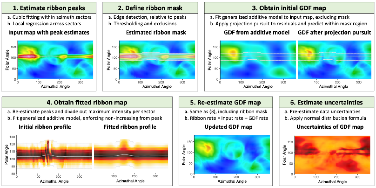
Figure 1: Illustration of the ribbon separation methods for a simulated input map (weak scattering model).¹

¹ The ribbon separation method is applied to a simulated ENA rate map derived from Zirnstein et al. (2019b) and Zirnstein et al. (2017) as described in Section 3 under assumptions of weak scattering. Images for steps 1-3 and 5 correspond to ENA rates between 0 (black) and 0.3 (red/magenta) ENAs per second. Images for step 4 correspond to scaled ENA profile intensities between 0 (white) and 1 (black). The image for step 6 corresponds to estimated GDF map standard errors between 0 (white) and 2.4e-4 (black). The ribbon mask is illustrated using a shaded horizontal band in images for steps 2-4. Estimated ribbon peaks are also shown as a near-horizontal gray line in images for steps 1-4.

2.1.1 Estimating ribbon peaks and defining the ribbon mask

The goal of ribbon mask estimation is to identify a map region in which ribbon-related ENA rates may be non-negligible. A very conservative ribbon mask will contain the entire ribbon but would leave little data outside the masked region for estimating the GDF map shape under the ribbon, leading to sub-optimal ribbon separation. Conversely, a less conservative mask may preserve more data for GDF map estimation while failing to capture the entire ribbon. Therefore, care must be taken in defining a ribbon mask region to balance between these two opposing objectives.
Suppose we visualize the data in the ribbon center rotational frame as a heatmap with latitude/polar angle on the y-axis, longitude/azimuthal angle on the x-axis, and the ENA rate $\mathcal{M}$ captured by the color intensity as in Figure 1. The ENA ribbon manifests as a near-horizontal band of concentrated ENA emissions. To capture deviations from a perfectly horizontal ribbon band, we started by identifying the locations of the ribbon peaks within each longitude bin (called an azimuthal sector). Funsten et al. (2013) proposed estimating the ribbon peak within each azimuthal sector by fitting a Gaussian-type profile $A+Be^{-\frac{(x-x_{p})}{2\sigma^{2}}}$ to the ENA rates estimated across polar angles $x$ to estimate the polar angle $x_{p}$ associated with the highest ENA rate (i.e., the peak). However, this Gaussian-type ribbon profile can produce poor estimates of the ribbon peak locations when the ribbon is highly non-Gaussian (as is the case for at least one leading ribbon generation hypothesis; Zirnstein et al. (2019b)). Instead, we defined each sector’s ribbon peak location $x_{p}$ as the arg-maximum value from a cubic interpolation of the ENA rates within each sector, which provides a much more flexible ribbon profile fit. We then performed some additional outlier screening and modeling across azimuthal sectors for enhanced stability of the ribbon peak estimates, as detailed in Supp. Section C.
Fixing these estimated ribbon peak locations, we then used a data-driven strategy to define a ribbon mask region, by estimating windows of polar angles above and below the ribbon peaks likely to contain ribbon ENAs. One strategy for identifying the location of the ENA ribbon is to estimate how quickly the ENA emissions are changing as a function of polar angle, since the ENA ribbon is expected to vary more quickly (i.e., have higher spatial gradients) than the GDF (Funsten et al., 2013). Regions associated with changing behavior of spatial gradients are sometimes called edges, and many methods have been developed for identifying these edges on fixed spatial grids. We apply this same logic to identify map regions associated with the “foothills” of the ribbon “mountain range.”
Re-organizing the ENA rate map with longitude on the x-axis and distance from peak (rounded into pixels) on the y-axis, we applied a popular edge detection method called the Sobel operator (Kanopoulos et al., 1988), where higher Sobel values are associated with greater “edginess.” The ribbon mask was defined in terms of the narrowest window that captures all of the top $u^{th}$ percentile of gradient estimates within $v$ degrees of the ribbon peak, with an additional two pixels added on either side to ensure the entire ribbon is captured. Reasonable values for $u$ and $v$ for a given map were chosen by repeating the entire ribbon separation method several times for different values of $(u,v)$ and choosing the combination resulting in the “best” ribbon separation as described in Supp. Section H. Additional details about this mask estimation are provided in Supp. Section C.

2.1.2 Obtaining the initial GDF map estimate

Once the ribbon mask region was identified for a given $(u,v)$, we then used the input map ENA rates $\mathcal{M}$ outside the ribbon mask to predict the shape of the GDF under the ribbon. Many different methods can be used to estimate a spatially-varying response surface (Schwadron et al., 2018; Reisenfeld et al., 2021; Swaczyna et al., 2022). We propose a multi-step approach for obtaining an initial GDF map estimate, where we first estimated a very smooth spatial surface for the GDF using generalized additive modeling (GAM) and then refined these predictions using projection pursuit regression (PPR) (Wood, 2017; Friedman and Stuetzle, 1981). To fit the GAM, we used R package mgcv, which allows users to specify the spatial model structure and degree of smoothing (Wood et al., 2016). We implemented an isotrophic spherical analog to thin plate splines, which allows the fitted model to account for the spherical latitude/longitude structure of the data (Wahba, 1981; Wood, 2003). For this GAM estimation, we used a Gaussian regression family with a log link to ensure that fitted GDF values were non-negative, and we incorporated first- to fourth-order derivative penalization to ensure smoothness.
The GAM model alone produces an overly smoothed estimate of the GDF. In order to capture spatial features in more detail, we then considered the residuals between the input map $\mathcal{M}$ and the GAM model predictions outside the ribbon mask. These residuals were then modeled using PPR and the fitted residuals added to the GAM GDF map predictions. Because additional spatial structure to the residuals was sometimes evident at this point, we performed one additional iteration of the PPR residual fitting, where this time observations with larger residuals were up-weighted in the PPR estimation. The GAM and PPR predictions together where then used to estimate the GDF map values inside the ribbon mask region. Initial GDF map estimates outside the ribbon mask were set equal to $\mathcal{M}$. Rarely-observed negative initial GDF map estimates after PPR were truncated to zero.

2.1.3 Obtaining the fitted ribbon map estimate and re-estimating the GDF map

Subtracting the initial GDF map estimate from the input data $\mathcal{M}$, we could obtain an initial estimate for the ribbon ENA rates within the ribbon mask region. However, this initial estimated ribbon map inherited any lack of fit or poor predictive performance of the GDF map estimation, which sometimes resulted in various data artifacts and non-ribbon features to be evident in the initial ribbon map.
To address this issue, we estimated a new ribbon map by modeling the initial ribbon map, imposing additional assumptions regarding the ribbon shape as illustrated in Figure 1. Our ribbon modeling focused on a scaled version of the initial ribbon map, where ENA rates in each azimuthal sector were divided the estimated peak height for that sector. This scaling step allowed us to focus the modeling efforts on the ribbon shape/profile rather than its relative intensity, which also avoided unintentional and unrealistic smoothing of ribbon intensities across azimuthal sectors. The resulting fitted ribbon maps were much more robust to poor GDF map estimation and has fewer jagged artifacts.
Our modeling of the ENA ribbon relied on two key assumptions: (1) the ribbon ENA rates are non-increasing as a function of the polar distance from the ribbon peak and (2) the shape of the ribbon varies smoothly across azimuthal angles. The former assumption relates to the ribbon shape (up to proportionality), and the second assumption relates to the variability in this shape along the ribbon. Briefly, we estimated the fitted ribbon map using a generalized additive model applied to the scaled initial ribbon map estimate as detailed in Supp. Section C, parameterized in terms of the azimuthal angle and the polar distance from the ribbon peak. In the current implementation, rapid ribbon profile changes at a azimuthal spatial scale of less than 30 degrees were not allowed; however, this assumption can be easily modified. After fitting, we then multiplied the fitted ribbon profile map by the azimuthal sector-specific maximum ENA rates to obtain the fitted ENA rate map. This resulting fitted ribbon map broadly satisfies the ribbon shape assumptions and has reduced sensitivity to noise and other data anomalies relative to the initial ribbon map.
After ribbon map estimation, we then re-estimated the GDF map using data obtained by subtracting the fitted ribbon map from the input data map $\mathcal{M}$. GDF map estimation then proceeded as before (using GAM and PPR), but it did not mask out the ribbon region. The goal of this GDF map re-estimation was to use ENA rates observed in the ribbon mask region to inform GDF map estimates, allowing for a more accurate GDF map estimate in this ribbon region. This procedure resulted in an estimated final GDF map, $\mathcal{G}$. Subtracting this estimate from the input data, $\mathcal{M}$, we obtained the final ribbon map estimate, $\mathcal{R}$. Negative estimated $\mathcal{R}$ values were truncated at zero.

2.1.4 Estimating map uncertainties

Above, we focused on obtaining point estimates of the ribbon and GDF maps. In order to estimate corresponding standard errors, we leveraged normality assumptions and relied upon properties of multivariate normal distributions. Recall, $\mathcal{M}$ denotes the vectorized input map estimates and $\sigma^{2}_{\mathcal{M}}$ denotes the corresponding uncertainties, after rotation into the ribbon-centric rotational frame. Each input map was estimated using raw IBEX ENA detection data (or using simulated versions). Let vector $y$ denote the rate of ENAs per second observed by IBEX attributed to each pixel of the sky, after accounting for blurring due to the wide IBEX field of view (i.e., IBEX can capture ENAs originating from a range of latitudes/longitudes when pointed in a given direction). We assume $y_{i}\sim N(\mathcal{M}_{i},\sigma_{iY}^{2})$, where $y_{i}$’s are assumed to be conditionally independent.
We assume that input map $\mathcal{M}$ is the sum of a ribbon-only map $\mathcal{R}$ and GDF-only map $\mathcal{G}$ and that $\mathcal{R}$ and $\mathcal{G}$ are marginally independent and normally-distributed such that $\mathcal{R}\sim N(\mu_{R},\sigma_{iR}^{2})$ and $\mathcal{G}\sim N(\mu_{G},\sigma_{iG}^{2})$. Together, these assumptions imply

$$\left(\begin{array}[]{c}\mathcal{G}_{i}\\ \mathcal{R}_{i}\\ y_{i}\end{array}\right)\sim N\left(\left[\begin{array}[]{c}\mu_{iG}\\ \mu_{iR}\\ \mu_{iG}+\mu_{iR}\end{array}\right],\left[\begin{array}[]{ccc}\sigma_{iG}^{2}&0&\sigma_{iG}^{2}\\ 0&\sigma_{iR}^{2}&\sigma_{iR}^{2}\\ \sigma_{iG}^{2}&\sigma_{iR}^{2}&\sigma_{iG}^{2}+\sigma_{iR}^{2}+\sigma_{iY}^{2}\end{array}\right]\right),$$

where $\mu$ collectively denotes the elements of $\mu_{G}$ and $\mu_{R}$ and $\Sigma$ collectively denotes the elements of $\sigma_{G}^{2}$, $\sigma_{R}^{2}$, and $\sigma_{Y}^{2}$. Using properties of normal distributions, we can express the uncertainties of the separated maps conditional on the observed IBEX data as

$$Var\left(\left[\begin{array}[]{c}\mathcal{G}_{i}\\ \mathcal{R}_{i}\end{array}\right]\bigg{|}y_{i};\mu,\Sigma\right)=\frac{1}{\sigma_{iG}^{2}+\sigma_{iR}^{2}+\sigma_{iY}^{2}}\left[\begin{array}[]{cc}\sigma_{iG}^{2}\{\sigma_{iR}^{2}+\sigma_{iY}^{2}\}&-\sigma_{iG}^{2}\sigma_{iR}^{2}\\ -\sigma_{iG}^{2}\sigma_{iR}^{2}&\sigma_{iR}^{2}\{\sigma_{iG}^{2}+\sigma_{iY}^{2}\}\end{array}\right].$$ (Eq. 5)

This expression is a function of three unknowns: $\sigma_{iG}^{2}$, $\sigma_{iR}^{2}$, and $\sigma_{iY}^{2}$. If we can estimate each of these unknowns using other available information, then we can directly plug in these estimates to Eq. 5 to obtain estimates for the uncertainty of estimated $\mathcal{G}$ and $\mathcal{R}$. As detailed in Supp. Section A, we can approximate all three parameters as a function of $\sigma^{2}_{i\mathcal{M}}=Var(\mathcal{G}_{i}+\mathcal{R}_{i}|y_{i},\mu,\Sigma)$ (the uncertainty of the input map) and $Var(y_{i}|\mathcal{G}_{i}+\mathcal{R}_{i},\mu,\Sigma)$ (the uncertainty of observed IBEX data for the given pixel given the input map estimate). Uncertainty $Var(y_{i}|\mathcal{G}_{i}+\mathcal{R}_{i},\mu,\Sigma)$ is estimated using the raw IBEX data using the approach in Supp. Section A.
To gain greater intuition about this variance expression, we note that

$$Var(\mathcal{G}_{i}|y_{i};\mu,\Sigma)+Var(\mathcal{R}_{i}|y_{i};\mu,\Sigma)=Var(\mathcal{G}_{i}+\mathcal{R}_{i}|y_{i};\mu,\Sigma)+2\frac{\sigma_{iG}^{2}\sigma_{iR}^{2}}{\sigma_{iG}^{2}+\sigma_{iR}^{2}+\sigma_{iY}^{2}}.$$

Restated, the sum of the estimated uncertainties for the GDF-only and ribbon-only maps is greater than the uncertainty of the input map $\mathcal{M}$, where the term $2\frac{\sigma_{iG}^{2}\sigma_{iR}^{2}}{\sigma_{iG}^{2}+\sigma_{iR}^{2}+\sigma_{iY}^{2}}$ captures additional uncertainty due to the ribbon separation process. In contrast, most ribbon separation methods in the IBEX literature do not account for this additional source of uncertainty, leading to overly narrow 95% confidence intervals for the separated map estimates.

2.2 Estimating the ribbon center

Our ribbon separation method leverages the near-circular shape of the ribbon in three-dimensional space (as illustrated in Figure 2) along with a convenient data rotation defined by the latitude/longitude location of the circle’s center. In this section, we propose a strategy for estimating the ribbon center and corresponding uncertainty using input map $\mathcal{D}$ and corresponding uncertainties $\sigma_{D}^{2}$.
First, we clarify what we mean by the ribbon “center.” Suppose we view the ENA data collected in three-dimensional space in terms of a unit sphere. We can visualize the ENA ribbon as being a closed shape on the surface of the sphere organized nearly-symmetrically around a normal axis/line intersecting the sphere. We will formalize the ribbon “center” as the latitude and longitude in which this normal line intersects the sphere. Strictly speaking, this line will intersect the unit sphere in two places, and we will define the ribbon “center” as the point that lies closer in latitude and longitude to the ribbon among these two points.
Two complications to estimating this center are that (1) the “location” of the ribbon is not well-defined and (2) the ENA map $\mathcal{D}$ used for estimation is pixelated and estimated with error. To tackle the former problem, we build on existing work that defines the “location” of the ribbon on the sphere in terms of estimated ribbon peaks. We address the latter problem by repeating our center estimation procedure multiple times on ENA maps drawn from a multivariate normal distribution with an estimated covariance matrix. The multivariate correlation matrix is estimated as the Kronecker product of dimension-specific (latitude- and longitude-) correlation matrices estimated using the input map intensities.

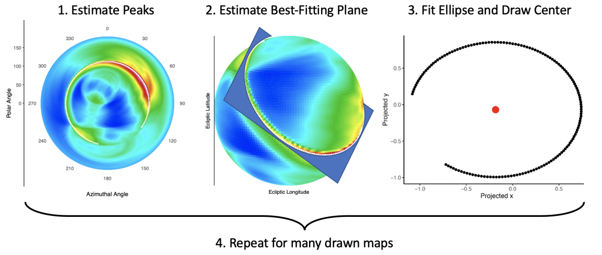
Figure 2: Visualization of proposed ribbon center estimation method, illustrated for a simulated GDF + ribbon weak scattering map. These methods can also be applied to ribbon-only map estimates. ¹

¹The first panel shows the same simulated input map as in Figure 1, visualized in polar coordinates. The ENA ribbon is visible as a near-circular band of enhanced ENA intensity, and the estimated ribbon peaks are shown as small white dots along the ribbon. The second panel illustrates the best fitting plane passing through these peak points in three dimensions. The third panel illustrates these peak points projected onto the best fitting plane and the corresponding estimated ellipse center (red dot). This ellipse center is converted to a latitude/longitude ribbon center location on the surface of the unit sphere by calculating the intersection between unit sphere and a line passing through the estimated ellipse center (in the plane) that is perpendicular to the best fitting plane. In the third panel, this perpendicular line would point directly out of the page.

Figure 2 provides an illustration of the proposed ribbon center estimation procedure. We start by defining an initial “working” estimate for the ribbon center and rotating each drawn ENA map into a working rotational frame, in which the ribbon center sits at the North pole. We then perform the following for each rotated, drawn ENA map:

1. Estimate the ribbon peak location for each azimuthal sector using the method in Supp. Section C.

2. Estimate the best fitting plane through these peak points using singular value decomposition as described in Blum et al. (2015). Project the peak points onto the best fitting plane using Rodrigues vector rotation (Dai, 2015).

3. Fit an ellipse using the fitConic package in R (Fitzgibbon et al., 1999). Then, estimate the covariance matrix associated with the ribbon center Cartesian coordinates in the plane using leave-one-out jackknife estimation (Efron and Stein, 1981).

4. Finally, draw Cartesian coordinates for the ellipse center in the plane from a bivariate normal distribution and calculate the corresponding latitude and longitude on the unit sphere (i.e., the ribbon center) in which the unit sphere intersects a normal line passing through the ellipse center in the best fitting plane.

This entire procedure is repeated many times to obtain many draws for the ribbon center latitude and longitude in ecliptic coordinates. These draws are treated as pseudo-posterior draws for the ribbon center longitude and latitude for inference. The means of these values provide our overall ribbon center location estimate. As demonstrated later on, we recommend iterating this process several times, using the estimated ribbon center to define the new working rotational frame each iteration. Additional details about the ribbon center estimation method are provided in Supp. Section E.

2.3 Spherical reference frame manipulation

Ribbon separation and ribbon center estimation involve recasting the data in different spherical reference frames. However, a pixelated three-dimensional map in one reference frame will become distorted and stretched when directly recast into a new reference frame using standard Davenport rotation (Davenport, 1968). To maintain the latitude/longitude pixelation structure after coordinate transformation, we propose (1) partitioning the new target frame latitude/longitude pixels (e.g., into 15 x 15 micropixels per pixel), (2) obtaining the ENA rate and uncertainty in the original frame for the midpoint of each micropixel, and (3) calculating the target pixel’s final ENA rate and uncertainty as the mean of the corresponding pointwise ENA rates and uncertainties associated with each pixel’s micropixels. This approach is appealing in that it preserves the same pixel structure in the original and target frames while avoiding re-estimating an entirely new ENA map in the new frame.
The performance of the ribbon separation method may depend on the choice of reference frame. The proposed separation methods leverage a near-horizontal structure of the ribbon in a rotational frame in which the ribbon “center” sits at the north pole. A very poorly specified rotational frame (i.e., a very bad estimate of the ribbon center), will make the ribbon separation model assumptions less reasonable. In practice, we guard against this possibility by performing ribbon separation using the rotational frame defined by the estimated ribbon center and by allowing the polar location of the ribbon peaks to vary smoothly across azimuthal angles.

3 Ribbon separation and center estimation in simulated data

We evaluated the performance of the proposed map separation and ribbon center estimation methods in simulated data, under three different simulation scenarios:

1. Weak scattering model

2. Spatial retention model

3. Smoothly varying ribbon profile model between spatial retention and weak scattering,

where physics simulation models were used to generate the spatial retention and weak scattering (i.e., the two leading ribbon formation hypotheses) profile shapes. In each scenario, the true total ENA rate map was defined as the sum of independently-simulated globally-distributed flux and ribbon maps.
For the first two simulation scenarios, the globally-distributed flux map was generated using a scaled version of the 2.73 keV GDF simulation from Zirnstein et al. (2017). Corresponding ribbon-only maps were generated to mimic the expected shape of the ribbon under two leading ribbon generation hypotheses as detailed in Zirnstein et al. (2019b), where the ribbon shape was determined using a single representative simulation cross-section and where the ribbon was assumed to be exactly circular and centered at longitude 221.5 and latitude 39. Dimming was added to certain sections of the ribbon to mirror observed IBEX data. For scenario S3, we considered a more complicated structure for the ribbon and GDF maps, including a spatially-varying ribbon shape, spatially concentrated knots on the ribbon, and a large high-flux disc on the GDF. Scenario S3 is not believed to be realistic; rather, this simulated scenario was devised to help characterize the limitations of the proposed ribbon separation and center estimation methods.
Under each of scenarios S1-S3, we performed ribbon separation using several different types of pixelated total ENA rate maps. First, we considered “ideal” input maps equal to the sum of the simulation truth ribbon-only and GDF-only maps. Unlike these idealized input maps, any total ENA rate maps generated using real IBEX data must overcome additional data challenges including substantial blurring, undesired background due to heliospheric ENAs, and missing data. To evaluate our methods in more realistic, messy data settings, we simulated data mimicking IBEX observed data and added background interference and blurring. Using these messy observed data, we applied an existing map construction strategy to obtain a set of pixel-level ENA rate estimates and uncertainties (Osthus et al., 2022). Results based on these messier input maps inherit any errors or biases induced by the upstream map-making procedure. This process resulted in a second set of “estimated” input maps. Finally, we estimated maps based on simulated data with 3 times longer observation time for each pixel of the sky, resulting in a third set of “estimated, 3x” input maps. The motivation for including this third set of maps was to mimic an emerging IBEX data product expected to result in substantial improvements in total ENA rate estimation accuracy (unpublished).

3.1 Ribbon separation performance

For each simulation scenario and each of three input maps (simulation truths and two sets of messier constructed maps), we applied the proposed map partitioning method described in Section 2.1. For comparison, we also implemented the ribbon separation methods proposed in Reisenfeld et al. (2021). We used a multi-faceted approach for assessing ribbon separation performance, including visual inspection of separated maps (Section 3.1.1); percent error, correlation, and weighted interval score (Bracher et al., 2021) comparing separated GDF map estimates and simulation truths (Section 3.1.2); ribbon skewness for separated ribbon maps and simulation truths; and visual comparison of estimated ribbon morphology (Section 3.1.3). Additional evaluations are provided in Supp. Section D.
We calculated the weighted interval score for pixel $i$ using the equation:

$$\text{WIS}_{i} =\frac{1}{M+0.5}\left[|\hat{\mathcal{G}}_{i}-\mathcal{G}_{i}|+\sum_{m=1}^{M}\frac{\alpha_{m}}{2}|\hat{u}_{im}-\hat{l}_{im}|+\sum_{m=1}^{M}(\hat{l}_{im}-\mathcal{G}_{i})^{I(\mathcal{G}_{i}<\hat{l}_{im})}(\mathcal{G}_{i}-\hat{u}_{im})^{I(\mathcal{G}_{i}>\hat{u}_{im})}\right]$$

where $\hat{\mathcal{G}}_{i}$ is the estimated GDF map, where $\mathcal{G}_{i}$ is the true value of the GDF, and where $\hat{l}_{im}$ and $\hat{u}_{im}$ are the $(1-\alpha_{m}/2)$% lower and upper confidence interval estimates, respectively. This weighted interval was averaged for all pixels with polar angles between 80 and 130, the region where both ribbon and GDF are potentially present. The weighted interval scores were calculated using $\alpha=(0.02,0.05,0.1,0.2,...,0.8,0.9)$.

3.1.1 Visual evaluation of ribbon separated maps

In Figure 3, we present the GDF and ribbon-only maps obtained by applying the proposed methods to each of the three “ideal” input datasets in the ecliptic rotational frame. Corresponding maps in the ribbon-centric frame and/or based on estimated input maps are presented in Supp. Figure D1. In settings S1/S2, the ribbon separations appear very clean, with little evidence of ribbon-related artifacts in the GDF-only map. For scenario S3, the region formerly containing the ribbon is visible in the GDF maps through residual banding, blurring, and other artifacts. As shown in Supp. Figure D2, maps produced using the methods in Reisenfeld et al. (2021) show even more pronounced banding and other artifacts across all simulation scenarios.

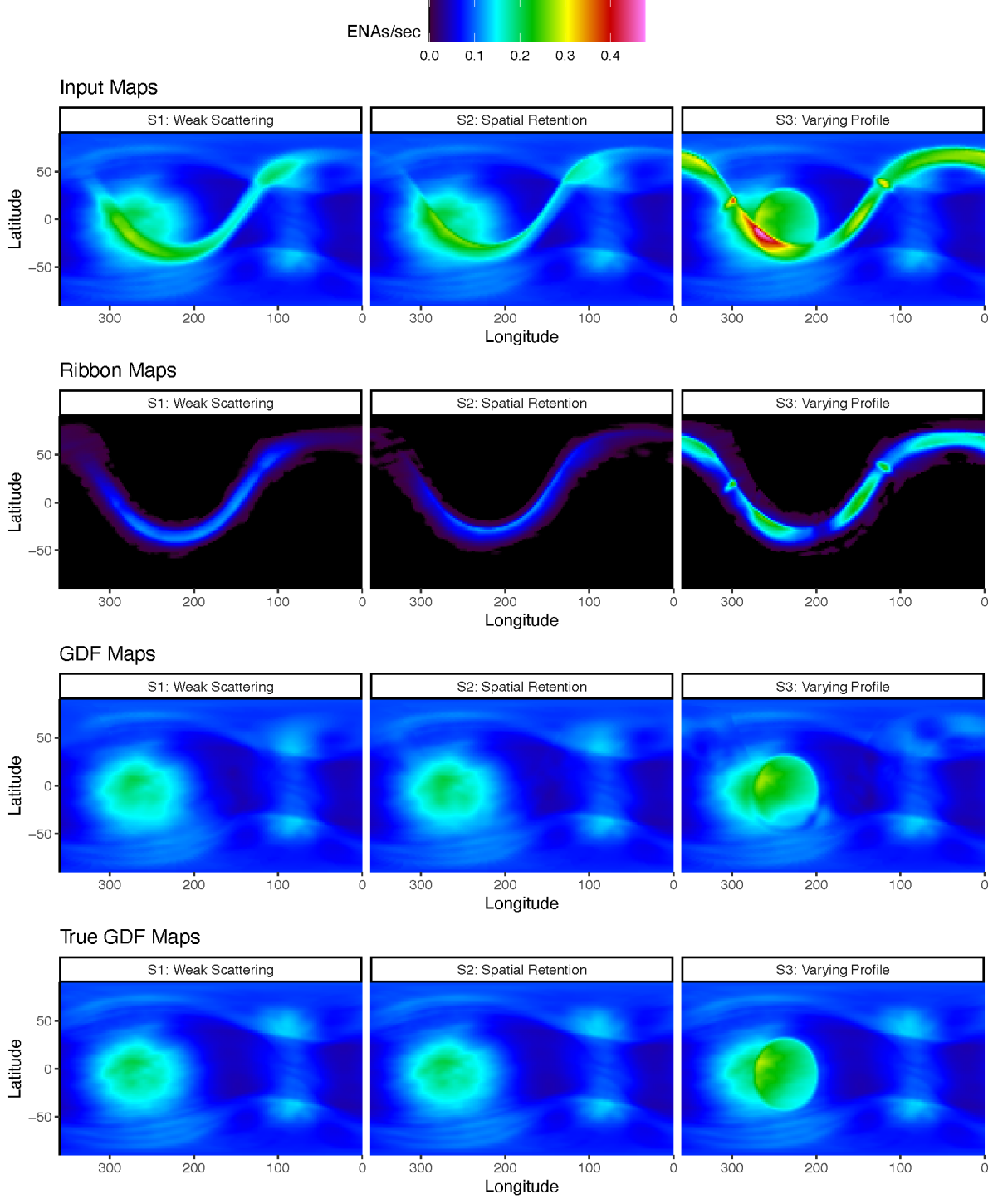
Figure 3: Estimated ribbon and GDF maps obtained using the proposed ribbon separation method applied to “ideal” (not estimated) simulated input maps¹.

¹ This figure shows simulated map partitions obtained using the method proposed in Section 2. Results are shown in the ecliptic rotational frame.

3.1.2 Accuracy and uncertainty of posterior GDF maps

We provide a more rigorous evaluation of the simulated map separation in Figure 4d. To summarize overall, the proposed ribbon separation performed well, outperforming the existing method in Reisenfeld et al. (2021) across nearly all metrics and simulation scenarios considered.
In the first panel of Figure 4d, we present the average percent error in GDF estimates in the ribbon region, and we provide the correlation between the true and estimated GDF values in the second panel. The proposed method resulted in high correlation between true and estimated GDF values across all simulation scenarios. Correlations for the method in Reisenfeld et al. (2021) were also high, but appreciably lower than the proposed method for most maps. The proposed method also resulted in much lower absolute percent error (by 30-60% for ideal inputs) than the method in Reisenfeld et al. (2021) across all simulation scenarios and input datasets considered.
The first two panels of Figure 4d focus only on estimated GDF and ribbon map values, but we are also interested in evaluating the corresponding standard errors. In the third panel, we present the estimated GDF map weighted interval score, which is a function of both the estimation error and corresponding uncertainties. Lower values of this score indicate better performance. The proposed method produced lower values for nearly all simulation scenarios and input map formulations. Scenario S3 using an estimated input map was the exception, where the weighted interval score was slightly better on average for the method in Reisenfeld et al. (2021).
The fourth panel of Figure 4d provides coverage of 95% confidence intervals for the GDF map estimates. Coverages for nearly all scenarios (and scenario S3 in particular) were substantially below the nominal 0.95 for estimated data maps. Under-coverage of the proposed method was a combination of two main factors: (1) error in the ribbon separation and (2) slight under-coverage of the estimated input map uncertainties. This issue is discussed in more detail in Supp. Section G. It is difficult to evaluate whether the proposed variance estimation results in “correct” coverage in a statistical sense due to the inherent lack of identifiability of the ribbon/GDF partitioning; this results in non-negligible bias even for excellent ribbon separations, since zero bias is not an achievable goal without strong ribbon shape assumptions that result in under-performance/lack of robustness in real data. In spite of this, our results do demonstrate similar or better statistical coverage relative to the method in Reisenfeld et al. (2021).

Figure 4: Performance of ribbon separation methods in terms of comparisons between estimated and true $GDF$ maps in the ribbon region¹

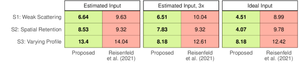
(a) Average absolute percent error between true and estimated GDF maps (lower = better)

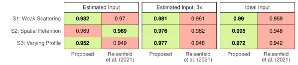
(b) Spearman correlation between true and estimated GDF maps (higher = better)

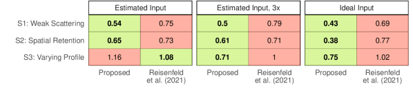
(c) Average weighted interval score between true and estimated GDF maps (lower = better)

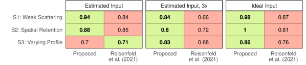
(d) Coverage of 95% confidence intervals of GDF map estimates (closer to 0.95 = better)

3.1.3 Visual comparison of ribbon profile shapes and skewness diagnostics

In addition to accuracy of the individual pixels in the separated maps, we are also interested in the overall profile or shape of the estimated ribbon. This is particularly relevant to downstream hypothesis testing between competing physics models explaining ribbon generation.
In Figure 5b, we compare ribbon cross-section estimates obtained using the proposed methods to the simulation truth for each azimuthal sector. Using ideal input maps, the proposed separation method captures the bent “shoulder” structure for scenario S2 and results in high fidelity to simulation truths for scenarios S1/S2. In scenario S3, the ribbon cross-sections do a good job of capturing the changing shape of the ribbon but do a poor job at estimating the ribbon shape for azimuthal angles above 300. The fitted ribbon shapes from the proposed method are much more accurate than those obtained using the method in Reisenfeld et al. (2021), which tends to smooth over nuance in the ribbon profile. In all simulation scenarios, ribbon profiles based on estimated (rather than ideal) input maps did not clearly have these distinguishing morphological features when not present in the input map.
Skewness could be potentially useful for discriminating between competing ribbon generation physics models, since the weak scattering and spatial retention physics models are believed to be associated with different ribbon skewness properties (Zirnstein et al., 2019a). In Supp. Figure D5, we compare estimated skewness in our separated ribbon maps with the simulation truth. The symmetric ribbon assumptions made by Reisenfeld et al. (2021) translated into near-symmetrical ribbon maps, meaning that hypothesis discrimination based on skewness is futile for those maps. The proposed maps resulted in skewness estimates that were biased toward zero relative to the simulation truth but that did capture differences between the two physics models in terms of skewness for ideal input maps. Skewness-based discrimination between physics model was less clear for estimated input maps. Similar diagnostics for the ribbon widths (full width at half max) are provided in Supp. Figure D6.

Figure 5: Spaghetti plots of ribbon/GDF map cross-sections by azimuthal sector for ideal (not estimated) input maps across different simulation scenarios. Results are shown using the proposed method and the method in Reisenfeld et al. (2021). ¹

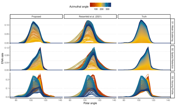
(a) Ribbon Map Estimates

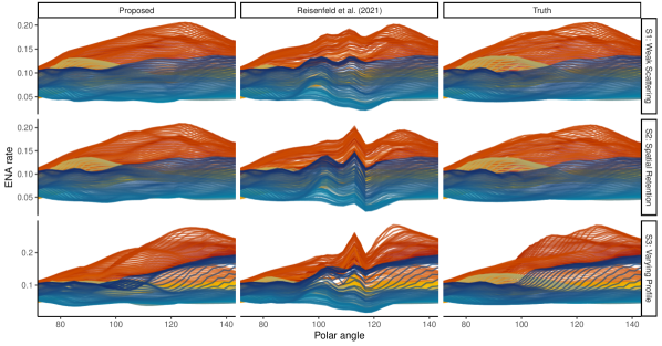
(b) GDF Map Estimates

¹This figure shows the estimated $\hat{\mathcal{R}}_{i}$ and $\hat{\mathcal{G}}_{i}$ values obtained for each simulation scenario, using ideal (i.e., not estimated) input maps. Lines correspond to cross-sections of ENA rates across different azimuthal sectors within each map.

3.2 Ribbon center estimation performance

For each set of maps under each of the three ribbon profile scenarios, we applied the proposed ribbon center method described in Section 2.2 to estimate the location of the ribbon center and its corresponding uncertainty. For comparison, we also implemented the method proposed in Funsten et al. (2013), which has several drawbacks relative to our proposed method. In particular, it does not account for input map estimation uncertainty, it models the ribbon profile using a Gaussian structure, and it performs the ellipse estimation in the working ribbon center frame only. Unless otherwise specified, the working ribbon center was set equal to the simulation truth. In all scenarios, the true ribbon center was located at longitude 221.5 and latitude 39 in the ecliptic frame.
In nearly all scenarios, the proposed ribbon center estimation method resulted in similar or lower bias and more reasonable uncertainty estimates than the method from Funsten et al. (2013). Figure 6b shows the estimated ribbon center latitudes and longitudes when estimation used the correct working frame, along with corresponding uncertainty ellipses. For scenarios S1/S2, error in ribbon center estimates were less than 0.5 degrees for all “ideal” (i.e., not estimated) simulated maps. Ribbon center estimation using the total flux map (i.e., with Ribbon + GDF) resulted in slightly higher estimation error than ribbon center estimation using separated ribbon-only maps. Uncertainty ellipses for the proposed method tended to be substantially larger than those estimated by Funsten et al. (2013). This is because the proposed methods captured uncertainty due to both the input map estimation and the ribbon center estimation for a fixed input map; the method in Funsten et al. (2013) accounts only for the latter.
With ideal input maps, the method in Funsten et al. (2013) outperformed the proposed method for scenario S3. This is because the proposed method produced better (in this case, more extreme) estimates of the ribbon peaks; however, the ribbon peaks turned out to be a poor proxy for ribbon location in scenario S3, with better peak estimates counter-intuitively leading to worse ribbon center estimates. This result provides a cautionary example highlighting that different metrics may be needed for characterizing the ribbon location in settings where the ribbon changes shape/skewness dramatically across azimuthal angles.
All estimates in Figure 6b assumed the correct working frame, but we would not expect the working frame to be correctly specified in general. When the working ribbon center was poorly specified, the downstream Funsten et al. (2013) ribbon center estimates showed substantial bias (Supp. Figure E2). Sensitivity of both methods to the working rotational frame was substantially mitigated by iterating the ribbon center estimation (Supp. Figure E3).

Figure 6: Performance of ribbon center estimation in simulated data¹

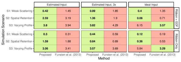
(a) Euclidean distance between estimated ribbon center and truth (degrees)

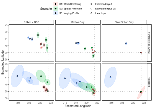
(b) Ribbon center estimates and 95% confidence ellipses

¹ This first panel of this figure shows the distance between ribbon center estimates and (221.5, 39), for ribbon center estimates obtained using the proposed method in Section 2.2 and using the method in Funsten et al. (2013). Lower values indicate more accurate ribbon center point estimates. All estimates are calculated using the correct rotational frame, where the true ribbon center in each simulated map is located at (221.5, 39) in ecliptic coordinates. The second panel of this figure shows the corresponding ribbon center estimates and 95% confidence ellipses. In both panels, “Ribbon + GDF” indicates estimation on the estimated or simulation truth map with both ribbon and GDF. “Ribbon-Only” refers to center estimation using maps that have been ribbon separated using the method in Section 2.1. “True Ribbon Only” refers to center estimation using the simulation truth ribbon-only map.

4 Application to real IBEX data

We applied the proposed ribbon center estimation and separation methods to 2-degree resolution real IBEX data maps generated using the method in Osthus et al. (2022). Ribbon center estimates along with detailed exploration of the ribbon-only and GDF-only maps will be presented in follow-up work. In this work, we provide some simple visual illustrations of the results of ENA ribbon separation.
Figure 7c shows the ribbon separation using the proposed method for data measured in 2019 for energy step 4 in the ram direction (the direction in which the sun is moving with respect to interstellar space). This map is a fairly representative example of the map separation performance for energy steps 3-5. All separated maps for energy step 4 are provided in Supp. Figure F2. Basic visual assessment reveals minimal banding or other artifacts along the ribbon region. Crucially, the separated maps appear to preserve some fine-scale features of the GDF in the ribbon region, which is a spatial region of particular scientific interest. Ribbon separation was most challenging for energy steps 2 and 6. For energy step 6 in particular, the estimated ribbon maps were somewhat patchy, indicating poor discrimination between GDF and ribbon for these maps (not shown). Data collected at this energy step do not have a defined ribbon to separate, and poor discrimination for energy step 6 was also seen using the method in Reisenfeld et al. (2021) (not shown).

Figure 7: Example separated maps for real IBEX data¹

(a) Input Map

(b) Ribbon Map

(c) GDF Map

¹This figure shows the results of ribbon separation for 2-degree input maps generated using real IBEX data for 2019, energy step 4, ram direction. Results are based on maps in the spacecraft frame and include survival and efficiency corrections but not Compton-Getting corrections (Compton and Getting, 1935). The large enhancement in ENA rates in (c) corresponds to the “nose” of the heliosphere (i.e., the direction in which the sun is moving with respect to interstellar space.

Figure 8a provides the ribbon skewness and width (measured by full width at half max; FWHM) for the ribbon-only map estimates within each azimuthal angle. These results reveal a fairly symmetrical ribbon on average, with some slight negative skewness (more ENA flux toward ribbon center) for ESAs (energy steps) 3-5. Estimated widths were the smallest for ESAs 3 and 4 on average, with median estimates of 26.2, 18.5, 16.5, 27.8, and 36.8 degrees, respectively, for ESAs 2-6 across all ram maps.
Figure 8b provides the maximum estimated ribbon ENA rate over time by energy step. Across ESAs, the method in Reisenfeld et al. (2021) tended to produce slightly dimmer ribbons than the proposed methods, likely due to the more restrictive ribbon shape assumed by Reisenfeld et al. (2021). However, changes in the ribbon heights over time and by ESA tended to be qualitatively similar between the proposed and Reisenfeld et al. (2021) methods (not shown). Both methods indicated that the ribbon intensity changed dramatically between 2009 and 2019, with much weaker ribbon flux from roughly 2015 to 2018.

Figure 8: Estimated ribbon morphology using real IBEX ram-only data by energy step (ESA) ¹

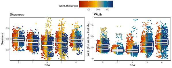
(a) Skewness and width (full width at half max) of estimated ribbon profiles by azimuthal sector across 105 separated ram maps (21 maps per ESA)

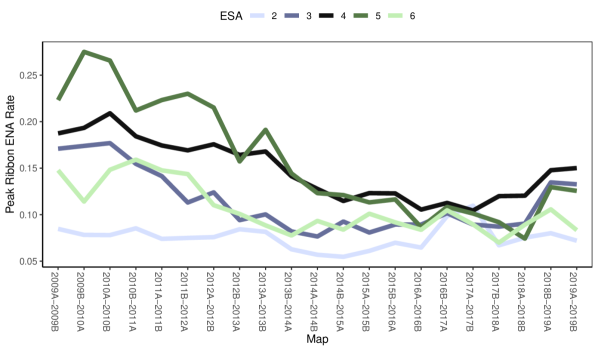
(b) Maximum estimated ribbon ENA rates over time by energy step (ESA) for ram-only maps

¹The first panel shows the estimated skewness and width (full width at half max) of ribbon map profiles for each of 180 azimuthal sectors for each of 105 2-degree maps generated using real IBEX data (overlapping yearly intervals between 2009 and 2019, energy steps 2-6, ram only). ‘A’ and ‘B’ correspond to the first and second half of each year, respectively. The full width at half max was estimated by fitting a cubic interpolation for each azimuthal angle and identifying the most extreme polar angles (at the 0.01 degree resolution) with predictions at least 50% of the azimuthal sector max. The second panel shows the point estimate for the highest estimated ribbon ENA rates for each map.

5 Discussion

Humanity is just beginning to understand the nature of the boundary between our solar system and interstellar space. Energetic neutral atoms (ENAs), primarily generated in this boundary heliosheath region, may provide important insight on the temporal and spatial variation in the shape and location of the heliosheath. Through the Interstellar Boundary Explorer (IBEX) mission, NASA collects data on the intensity of these ENA particles over the full sky. These data have been used to construct pixelated maps of the observed ENA flux.
ENAs captured by these maps are believed to primarily originate from two separate processes, and these two sources of ENAs and corresponding ENA intensities are each of scientific interest. Therefore, a key step of IBEX data processing is partitioning into separate maps representing both ENA types: globally-distributed flux (GDF) and the ENA “ribbon.” In this work, we proposed a new statistical method for partitioning ENA maps into source-specific maps. Ancillary to this goal is estimation of the so-called ribbon “center”, and we also developed methods to perform this estimation. The performance of the proposed methods was evaluated using simulated data designed to mimic observed IBEX data and compared against leading alternative methods in the scientific literature.
We found that the flexible proposed ribbon separation method had excellent performance in terms of the accuracy of map partitioning and the ability to capture nuances in ribbon morphology. The gains in performance of the proposed method over the ribbon separation method in Reisenfeld et al. (2021) substantially increased as the quality of the input data improved, primarily because key subtle features of ribbon morphology where smoothed out or entirely absent in lower-quality maps. In terms of IBEX mission data processing, our results support development and use of high-quality, high-resolution IBEX data products such as the finely resolved 2-degree ENA maps developed in Osthus et al. (2022) and recently-generated maps incorporating multiple types of ENA encounters (unpublished).
In addition to map separation, we also proposed new methods for estimating the “center” of the ENA ribbon and these methods showed good performance in simulated data analyses. Our results demonstrated that iteration is key; a single iteration of ribbon center estimation can result in substantial residual bias for both the proposed method and, to an even greater degree, the method in Funsten et al. (2013).
Our initial application of these methods to real IBEX data indicated that the ENA ribbon cross-sections tended to have a slight negative skewness for energy passbands (ESAs) 3-5. The width of the ENA ribbon also varied by ESA, with the narrowest ribbon profiles observed for ESA 4 on average. Temporal changes in the ribbon intensity were also observed. Future work will explore implications of these temporal and energy passband-related variations in more detail.
The ultimate goal of the proposed methods was to provide a concrete, quantifiable advance in the quality of the IBEX source-specific maps used for downstream scientific research into the complicated physics operating at the edges of our solar system. Additionally, this work illustrates the potential for statistical thinking to substantially contribute to scientific understanding. As more complicated and nuanced scientific data become available through advances in technology and computing, partnerships between data experts and scientific domain experts will be hugely important to facilitate scientific discovery.

6 Acknowledgments

This work was partially funded by the Laboratory Directed Research and Development (LDRD) Project 20220107DR. Dr. Beesley was also funded by the LDRD Richard Feynman Postdoctoral Fellowship 20210761PRD1. This work is approved for distribution under LA-UR-22-32267.

References

- Blum et al. (2015) Avrim Blum, John Hopcroft, and Ravindran Kannan. Foundations of Data Science. Cambridge University Press, 2015.
- Bracher et al. (2021) Johannes Bracher, Evan L. Ray, Tilmann Gneiting, and Nicholas G. Reich. Evaluating epidemic forecasts in an interval format. PLoS Computational Biology, 17:1–15, 2021. doi: 10.1371/JOURNAL.PCBI.1008618.
- Compton and Getting (1935) Arthur H. Compton and Ivan A. Getting. An apparent effect of galactic rotation on the intensity of cosmic rays. Physical Review, 47, 1935. ISSN 0031899X. doi: 10.1103/PhysRev.47.817.
- Dai (2015) Jian S Dai. Euler–rodrigues formula variations, quaternion conjugation and intrinsic connections. Mechanism and Machine Theory, 92:144–152, 2015.
- Davenport (1968) Paul B Davenport. A vector approach to the algebra of rotations with applications, 1968.
- Dayeh et al. (2019) M. A. Dayeh, E. J. Zirnstein, M. I. Desai, H. O. Funsten, S. A. Fuselier, J. Heerikhuisen, D. J. McComas, N. A. Schwadron, and J. R. Szalay. Variability in the position of the ibex ribbon over nine years: More observational evidence for a secondary ena source. The Astrophysical Journal, 879:84, 7 2019. ISSN 0004-637X. doi: 10.3847/1538-4357/ab21c1.
- Efron and Stein (1981) B Efron and C Stein. The jackknife estimate of variance. The Annals of Statistics, 9:586–596, 1981.
- Fitzgibbon et al. (1999) Andrew Fitzgibbon, Maurizio Pilu, and Robert B. Fisher. Direct least square fitting of ellipses. IEEE Transactions on Pattern Analysis and Machine Intelligence, 21:476–480, 1999. ISSN 01628828. doi: 10.1109/34.765658.
- Friedman and Stuetzle (1981) Jerome H. Friedman and Werner Stuetzle. Projection pursuit regression. Journal of the American Statistical Association, 76, 1981. ISSN 1537274X. doi: 10.1080/01621459.1981.10477729.
- Funsten et al. (2009a) H. O. Funsten, F. Allegrini, P. Bochsler, G. Dunn, S. Ellis, D. Everett, M. J. Fagan, S. A. Fuselier, M. Granoff, M. Gruntman, A. A. Guthrie, J. Hanley, R. W. Harper, D. Heirtzler, P. Janzen, K. H. Kihara, B. King, H. Kucharek, M. P. Manzo, M. Maple, K. Mashburn, D. J. McComas, E. Moebius, J. Nolin, D. Piazza, S. Pope, D. B. Reisenfeld, B. Rodriguez, E. C. Roelof, L. Saul, S. Turco, P. Valek, S. Weidner, P. Wurz, and S. Zaffke. The interstellar boundary explorer high energy (ibex-hi) neutral atom imager. Space Science Reviews, 146:75–103, 8 2009a. ISSN 00386308. doi: 10.1007/s11214-009-9504-y.
- Funsten et al. (2009b) H O Funsten, F Allegrini, G B Crew, R DeMajistre, P C Frisch, S A Fuselier, M Gruntman, P Janzen, D J McComas, E Möbius, B Randol, D B Reisenfeld, E C Roelof, and N A Schwadron. Structures and spectral variations of the outer heliosphere in ibex energetic neutral atom maps. Space Sci. Rev, 326:2021, 2009b. doi: 10.1007/s11214.
- Funsten et al. (2013) H. O. Funsten, R. Demajistre, P. C. Frisch, J. Heerikhuisen, D. M. Higdon, P. Janzen, B. A. Larsen, G. Livadiotis, D. J. McComas, E. Möbius, C. S. Reese, D. B. Reisenfeld, N. A. Schwadron, and E. J. Zirnstein. Circularity of the interstellar boundary explorer ribbon of enhanced energetic neutral atom (ena) flux. Astrophysical Journal, 776, 10 2013. ISSN 15384357. doi: 10.1088/0004-637X/776/1/30.
- Kanopoulos et al. (1988) Nick Kanopoulos, Nagesh Vasanthavada, and Robert L Baker. Design of an image edge detection filter using the sobel operator. IEEE Journal of solid-state circuits, 23(2):358–367, 1988.
- McComas et al. (2009) D. J. McComas, F. Allegrini, P. Bochsler, M. Bzowski, E. R. Christian, G. B. Crew, R. DeMajistre, H. Fahr, H. Fichtner, P. C. Frisch, H. O. Funsten, S. A. Fuselier, G. Gloeckler, M. Gruntman, J. Heerikhuisen, V. Izmodenov, P. Janzen, P. Knappenberger, S. Krimigis, H. Kucharek, M. Lee, G. Livadiotis, S. Livi, R. J. MacDowall, D. Mitchell, E. Möbius, T. Moore, N. V. Pogorelov, D. Reisenfeld, E. Roelof, L. Saul, N. A. Schwadron, P. W. Valek, R. Vanderspek, P. Wurz, and G. P. Zank. Global observations of the interstellar interaction from the interstellar boundary explorer (ibex). Science, 326(5955):959–962, 2009. doi: 10.1126/science.1180906. URL https://www.science.org/doi/abs/10.1126/science.1180906.
- McComas et al. (2014) D. J. McComas, W. S. Lewis, and N. A. Schwadron. Ibex’s enigmatic ribbon in the sky and its many possible sources. Reviews of Geophysics, 52(1):118–155, 2014. doi: https://doi.org/10.1002/2013RG000438. URL https://agupubs.onlinelibrary.wiley.com/doi/abs/10.1002/2013RG000438.
- Osthus et al. (2022) Dave Osthus, Brian P. Weaver, Lauren J. Beesley, Kelly R. Moran, Madeline A. Ausdemore, Eric J. Zirnstein, Paul H. Janzen, and Daniel B. Reisenfeld. Towards improved heliosphere sky map estimation with theseus, 2022. URL https://arxiv.org/abs/2210.12005.
- Reisenfeld et al. (2021) Daniel B. Reisenfeld, Maciej Bzowski, Herbert O. Funsten, Jacob Heerikhuisen, Paul H. Janzen, Marzena A. Kubiak, David J. McComas, Nathan A. Schwadron, Justyna M. Sokół, Alex Zimorino, and Eric J. Zirnstein. A three-dimensional map of the heliosphere from ibex. The Astrophysical Journal Supplement Series, 254:40, 6 2021. ISSN 0067-0049. doi: 10.3847/1538-4365/abf658.
- Schwadron et al. (2011) N. A. Schwadron, F. Allegrini, M. Bzowski, E. R. Christian, G. B. Crew, M. Dayeh, R. Demajistre, P. Frisch, H. O. Funsten, S. A. Fuselier, K. Goodrich, M. Gruntman, P. Janzen, H. Kucharek, G. Livadiotis, D. J. McComas, E. Moebius, C. Prested, D. Reisenfeld, M. Reno, E. Roelof, J. Siegel, and R. Vanderspek. Separation of the interstellar boundary explorer ribbon from globally distributed energetic neutral atom flux. Astrophysical Journal, 731, 4 2011. ISSN 15384357. doi: 10.1088/0004-637X/731/1/56.
- Schwadron et al. (2014) N. A. Schwadron, E. Moebius, S. A. Fuselier, D. J. McComas, H. O. Funsten, P. Janzen, D. Reisenfeld, H. Kucharek, M. A. Lee, K. Fairchild, F. Allegrini, M. Dayeh, G. Livadiotis, M. Reno, M. Bzowski, J. M. Sokół, M. A. Kubiak, E. R. Christian, R. Demajistre, P. Frisch, A. Galli, P. Wurz, and M. Gruntman. Separation of the ribbon from globally distributed energetic neutral atom flux using the first five years of ibex observations. Astrophysical Journal, Supplement Series, 215, 10 2014. ISSN 00670049. doi: 10.1088/0067-0049/215/1/13.
- Schwadron et al. (2018) N. A. Schwadron, F. Allegrini, M. Bzowski, E. R. Christian, M. A. Dayeh, M. I. Desai, K. Fairchild, P. C. Frisch, H. O. Funsten, S. A. Fuselier, A. Galli, P. Janzen, M. A. Kubiak, D. J. McComas, E. Moebius, D. B. Reisenfeld, J. M. Sokół, P. Swaczyna, J. R. Szalay, P. Wurz, and E. J. Zirnstein. Time dependence of the ibex ribbon and the globally distributed energetic neutral atom flux using the first 9 years of observations. The Astrophysical Journal Supplement Series, 239:1, 10 2018. ISSN 00670049. doi: 10.3847/1538-4365/aae48e.
- Swaczyna et al. (2022) P. Swaczyna, T. J. Eddy, E. J. Zirnstein, M. A. Dayeh, D. J. McComas, H. O. Funsten, and N. A. Schwadron. Ibex ribbon separation using spherical harmonic decomposition of the globally distributed flux. The Astrophysical Journal Supplement Series, 258:6, 1 2022. ISSN 0067-0049. doi: 10.3847/1538-4365/ac2f47.
- Wahba (1981) Grace Wahba. Spline interpolation and smoothing on the sphere. SIAM Journal on Scientific and Statistical Computing, 2, 1981. ISSN 0196-5204. doi: 10.1137/0902002.
- Wood (2003) Simon N. Wood. Thin plate regression splines, 2003. ISSN 13697412.
- Wood (2017) Simon N. Wood. Generalized additive models: An introduction with R, second edition. 2017. doi: 10.1201/9781315370279.
- Wood et al. (2016) S.N. Wood, N., Pya, and B. S”afken. Smoothing parameter and model selection for general smooth models (with discussion). Journal of the American Statistical Association, 111:1548–1575, 2016.
- Zirnstein et al. (2015) E. J. Zirnstein, J. Heerikhuisen, N. V. Pogorelov, D. J. McComas, and M. A. Dayeh. Simulations of a dynamic solar cycle and its effects on the interstellar boundary explorer ribbon and globally distributed energetic neutral atom flux. The Astrophysical Journal, 804(1):5, apr 2015. doi: 10.1088/0004-637X/804/1/5. URL https://dx.doi.org/10.1088/0004-637X/804/1/5.
- Zirnstein et al. (2016) E. J. Zirnstein, J. Heerikhuisen, H. O. Funsten, G. Livadiotis, D. J. McComas, and N. V. Pogorelov. Local interstellar magnetic field determined from the interstellar boundary explorer ribbon. The Astrophysical Journal Letters, 818(1):L18, feb 2016. doi: 10.3847/2041-8205/818/1/L18. URL https://dx.doi.org/10.3847/2041-8205/818/1/L18.
- Zirnstein et al. (2017) E. J. Zirnstein, J. Heerikhuisen, G. P. Zank, N. V. Pogorelov, H. O. Funsten, D. J. McComas, D. B. Reisenfeld, and N. A. Schwadron. Structure of the heliotail from interstellar boundary explorer observations: Implications for the 11-year solar cycle and pickup ions in the heliosheath. The Astrophysical Journal, 836(2):238, feb 2017. doi: 10.3847/1538-4357/aa5cb2. URL https://dx.doi.org/10.3847/1538-4357/aa5cb2.
- Zirnstein et al. (2019a) E. J. Zirnstein, D. J. McComas, N. A. Schwadron, M. A. Dayeh, J. Heerikhuisen, and P. Swaczyna. Strong scattering of kev pickup ions in the local interstellar magnetic field draped around our heliosphere: Implications for the ibex ribbon’s source and imap. The Astrophysical Journal, 876, 2019a. ISSN 15384357. doi: 10.3847/1538-4357/ab15d6.
- Zirnstein et al. (2019b) E. J. Zirnstein, P. Swaczyna, D. J. McComas, and J. Heerikhuisen. Parallax of the ibex ribbon indicates a spatially retained source. The Astrophysical Journal, 879(2):106, jul 2019b. doi: 10.3847/1538-4357/ab2633. URL https://dx.doi.org/10.3847/1538-4357/ab2633.