Robust Subtask Learning for Compositional Generalization

Kishor Jothimurugan    Steve Hsu    Osbert Bastani    Rajeev Alur
Abstract

Compositional reinforcement learning is a promising approach for training policies to perform complex long-horizon tasks. Typically, a high-level task is decomposed into a sequence of subtasks and a separate policy is trained to perform each subtask. In this paper, we focus on the problem of training subtask policies in a way that they can be used to perform any task; here, a task is given by a sequence of subtasks. We aim to maximize the worst-case performance over all tasks as opposed to the average-case performance. We formulate the problem as a two agent zero-sum game in which the adversary picks the sequence of subtasks. We propose two RL algorithms to solve this game: one is an adaptation of existing multi-agent RL algorithms to our setting and the other is an asynchronous version which enables parallel training of subtask policies. We evaluate our approach on two multi-task environments with continuous states and actions and demonstrate that our algorithms outperform state-of-the-art baselines.

Machine Learning, ICML

1 Introduction

Reinforcement learning (RL) has proven to be a promising strategy for solving complex control tasks such as walking (Fujimoto et al., 2018), autonomous driving (Ivanov et al., 2021), and dexterous manipulation (Akkaya et al., 2019). However, a key challenge facing the deployment of reinforcement learning in real-world tasks is its high sample complexity—solving any new task requires training a new policy designed to solve that task. One promising solution is compositional reinforcement learning, where individual options (or skills) are first trained to solve simple tasks; then, these options can be composed together to solve more complex tasks (Lee et al., 2018, 2021; Ivanov et al., 2021). For example, if a driving robot learns how to make left and right turns and to drive in a straight line, it can then drive along any route composed of these primitives.

A key challenge facing compositional reinforcement learning is the generalizability of the learned options. In particular, options trained under one distribution of tasks may no longer work well if used in a new task, since the distribution of initial states from which the options are used may shift. An alternate approach is to train the options separately to perform specific subtasks, but options trained this way might cause the system to reach states from which future subtasks are hard to perform. One can overcome this issue by handcrafting rewards to encourage avoiding such states (Ivanov et al., 2021), in which case they generalize well, but this approach relies heavily on human time and expertise.

We propose a novel framework that addresses these challenges by formulating the option learning problem as an adversarial reinforcement learning problem. At a high level, the adversary chooses the task that minimizes the reward achieved by composing the available options. Thus, the goal is to learn a set of robust options that perform well across all potential tasks. Then, we provide two algorithms for solving this problem. The first adapts existing ideas for using reinforcement learning to solve Markov games to our setting. Then, the second shows how to leverage the compositional structure of our problem to learn options in parallel at each step of a value iteration procedure; in some cases, by enabling such parallelism, we can reduce the computational cost of learning.
Refer to caption
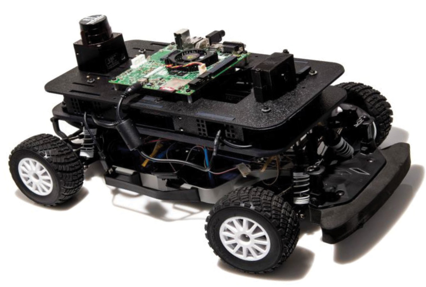
(a) F1/10th Car
Refer to caption
(b) Segment Types
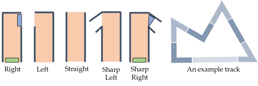
Figure 1: F1/10th Environment. The entry and exit regions for the right and sharp right segments are shown in green and blue respectively.

We validate our approach on two benchmarks: (i) a rooms environment where a point mass robot must navigate any given sequence of rooms, and (ii) a simulated version of the F1/10th car, where a small racing car must navigate any given racetrack that is composed of several different predefined track segments. In both environments, our empirical results demonstrate that robust options are critical for performing well on a wide variety of tasks.

In summary, our contributions are: (i) a game theoretic formulation of the compositional reinforcement learning problem, (ii) an algorithm for solving this problem in the finite-state setting with guaranteed convergence in the limit, (iii) two learning algorithms for continuous-state systems, and (iv) an empirical evaluation demonstrating the effectiveness of our approach.

Motivating example.

Let us consider a small scale autonomous racing car shown in Figure 1 (a). We would like to train a controller that can be used to navigate the car through all tracks constructed using five kinds of segments; the possible segments are shown in Figure 1 (b) along with an example track. A state of the car is a vector s=(x,y,v,θ)𝑠𝑥𝑦𝑣𝜃s=(x,y,v,\theta) where (x,y)𝑥𝑦(x,y) is its position on the track relative to the current segment, v𝑣v is its current speed and θ𝜃\theta is the heading angle. At any state s𝑠s, the controller observes the measurements o(s)1081𝑜𝑠superscript1081o(s)\in\mathbb{R}^{1081} of a LiDAR sensor and outputs an action (a,ω)2𝑎𝜔superscript2(a,\omega)\in\mathbb{R}^{2} where a𝑎a is the throttle input and ω𝜔\omega is the steering angle. In this environment, completing each segment is considered a subtask and a task corresponds to completing a sequence of segments (which may describe a track)—e.g., straightrightleftsharp-rightstraightrightleftsharp-right{\texttt{straight}}\to{\texttt{right}}\to{\texttt{left}}\to{\texttt{sharp-right}}. Upon completion of a subtask, the car enters the next segment and a change-of-coordinates111The change-of-coordinates is assumed for simpler modelling and does not affect the LiDAR measurements or the controller. is applied to the car’s state which is now relative to the new segment. The goal here is to learn one option for each subtask such that the agent can perform any task using these options.

If one trains the options independently with the only goal of reaching the end of each segment (e.g., using distance-based rewards), it might (and does) happen that the car reaches the end of a segment in a state that was not part of the initial states used to train the policy corresponding to the next segment. Therefore, one should make sure that the initial state distribution used during training includes such states as well—either manually or using dataset aggregation (Ross et al., 2011). Furthermore, it is possible that the car reaches a state in the exit region of a segment from which it is challenging to complete the next subtask—e.g., a state in which the car is close to and facing towards a wall. Our algorithm identifies during training that, in order to perform future subtasks, it is better to reach the end of a segment in a configuration where the car is facing straight relative to the next segment. Finally, we want the trained options to be such that they compose well for every sequence of segments—i.e., track geometry. Therefore, we are interested in maximizing the worst case performance with respect to the choice of high-level task.

Our framework is broadly applicable in many real-world scenarios. For instance, the F1/10th example can be seen as a miniature version of an autonomous driving scenario where the agent needs to learn to perform maneuvers such as turning left/right, changing lanes etc. Here, the policies for performing these maneuvers need to ensure that the car is in a safe and controllable state for future maneuvers. Another interesting scenario is when a household robot has to perform multiple tasks such as cleaning, cooking etc., but needs to ensure that the policies for performing these tasks leave the house in a favorable state for future tasks—e.g., learning to cook without making the place too dirty (as it might be hard to perform the cleaning task later).

2 Problem Formulation

A multi-task Markov decision process (MDP) is a tuple =(S,A,P,Σ,R,F,T,γ,η,σ0)𝑆𝐴𝑃Σ𝑅𝐹𝑇𝛾𝜂subscript𝜎0\mathcal{M}=(S,A,P,\Sigma,R,F,T,\gamma,\eta,\sigma_{0}), where S𝑆S are the states, A𝐴A are the actions, P(ss,a)[0,1]𝑃conditionalsuperscript𝑠𝑠𝑎01P(s^{\prime}\mid s,a)\in[0,1] is the probability of transitioning from s𝑠s to ssuperscript𝑠s^{\prime} on action a𝑎a, η𝜂\eta is the initial state distribution, and γ(0,1)𝛾01\gamma\in(0,1) is the discount factor. Furthermore, ΣΣ\Sigma is a set of subtasks and for each subtask σΣ𝜎Σ\sigma\in\Sigma, Rσ:S×A:subscript𝑅𝜎𝑆𝐴R_{\sigma}:S\times A\to\mathbb{R} is a reward function222We can also have a reward function Rσ:S×A×S:subscript𝑅𝜎𝑆𝐴𝑆R_{\sigma}:S\times A\times S\to\mathbb{R} that depends on the next state but we omit it for clarity of presentation., FσSsubscript𝐹𝜎𝑆F_{\sigma}\subseteq S is a set of final states where the subtask is considered completed and Tσ:Fσ×S[0,1]:subscript𝑇𝜎subscript𝐹𝜎𝑆01T_{\sigma}:F_{\sigma}\times S\to[0,1] is the jump probability function; upon reaching a state s𝑠s in Fσsubscript𝐹𝜎F_{\sigma} the system jumps to a new state ssuperscript𝑠s^{\prime} with probability Tσ(ss)subscript𝑇𝜎conditionalsuperscript𝑠𝑠T_{\sigma}(s^{\prime}\mid s). For the sake of clarity, we assume333This assumption can be removed by adding a fictitious copy of Fσsubscript𝐹𝜎F_{\sigma} to S𝑆S for each σΣ𝜎Σ\sigma\in\Sigma. that Tσ(ss)=0subscript𝑇𝜎conditionalsuperscript𝑠𝑠0T_{\sigma}(s^{\prime}\mid s)=0 for any ssuperscript𝑠s^{\prime} with sFσsuperscript𝑠subscript𝐹superscript𝜎s^{\prime}\in F_{\sigma^{\prime}} for some σsuperscript𝜎\sigma^{\prime}. Finally, σ0Σsubscript𝜎0Σ\sigma_{0}\in\Sigma is the initial subtask which has to be completed first444When there is no fixed initial subtask, we can add a fictitious initial subtask.. A multi-task MDP can be viewed as a discrete time variant of a hybrid automaton model (Ivanov et al., 2021).

In the case of our motivating example, the set of subtasks is given by Σ={left,right,straight,\Sigma=\{{\texttt{left}},{\texttt{right}},{\texttt{straight}}, sharp-left,sharp-right}{\texttt{sharp-left}},{\texttt{sharp-right}}\} with Fσsubscript𝐹𝜎F_{\sigma} denoting the exit region of the segment corresponding to subtask σ𝜎\sigma. We use the jump transitions T𝑇T to model the change-of-coordinates performed upon reaching an exit region. The reward function Rσsubscript𝑅𝜎R_{\sigma} for a subtask σ𝜎\sigma is given by Rσ(s,a,s)=scσ22+B𝟙(sFσ)subscript𝑅𝜎𝑠𝑎superscript𝑠superscriptsubscriptdelimited-∥∥superscript𝑠subscript𝑐𝜎22𝐵1superscript𝑠subscript𝐹𝜎R_{\sigma}(s,a,s^{\prime})=-{\lVert s^{\prime}-c_{\sigma}\rVert}_{2}^{2}+B\cdot\mathbbm{1}(s^{\prime}\in F_{\sigma}) where cσsubscript𝑐𝜎c_{\sigma} is the center of the exit region and the subtask completion bonus B𝐵B is a positive constant.

A task τ𝜏\tau is defined to be an infinite sequence555A finite sequence can be appended with an infinite sequence of fictitious subtasks with zero reward. of subtasks τ=σ0σ1𝜏subscript𝜎0subscript𝜎1\tau=\sigma_{0}\sigma_{1}\ldots, and 𝒯𝒯\mathcal{T} denotes the set of all tasks. For any task τ𝒯𝜏𝒯\tau\in\mathcal{T}, τ[i]𝜏delimited-[]𝑖\tau[i] denotes the ithsuperscript𝑖thi^{\text{th}} subtask σisubscript𝜎𝑖\sigma_{i} in τ𝜏\tau. In our setting, the task is chosen by the environment nondeterministically. Given a task τ𝜏\tau, a configuration of the environment is a pair (s,i)S×0𝑠𝑖𝑆subscriptabsent0(s,i)\in S\times\mathbb{Z}_{\geq 0} with sFτ[i]𝑠subscript𝐹𝜏delimited-[]𝑖s\notin F_{\tau[i]} denoting that the system is in state s𝑠s and the current subtask is τ[i]𝜏delimited-[]𝑖\tau[i]. The initial distribution over configurations Δ:S×0[0,1]:Δ𝑆subscriptabsent001\Delta:S\times\mathbb{Z}_{\geq 0}\to[0,1] is given by Δ(s,i)=ητ[0](s)Δ𝑠𝑖subscript𝜂𝜏delimited-[]0𝑠\Delta(s,i)=\eta_{\tau[0]}(s) if i=0𝑖0i=0 and 00 otherwise. The probability of transitioning from (s,i)𝑠𝑖(s,i) to (s,j)superscript𝑠𝑗(s^{\prime},j) on an action a𝑎a is given by Pr((s,j)(s,i),a)=Prconditionalsuperscript𝑠𝑗𝑠𝑖𝑎absent\Pr((s^{\prime},j)\mid(s,i),a)=

{s′′Fτ[i]P(s′′s,a)Tτ[i](ss′′)ifj=i+1P(ss,a)ifj=i&sFτ[i]0otherwise.casessubscriptsuperscript𝑠′′subscript𝐹𝜏delimited-[]𝑖𝑃conditionalsuperscript𝑠′′𝑠𝑎subscript𝑇𝜏delimited-[]𝑖conditionalsuperscript𝑠superscript𝑠′′if𝑗𝑖1𝑃conditionalsuperscript𝑠𝑠𝑎if𝑗𝑖superscript𝑠subscript𝐹𝜏delimited-[]𝑖0otherwise.\displaystyle\begin{cases}\sum_{s^{\prime\prime}\in F_{\tau[i]}}P(s^{\prime\prime}\mid s,a)T_{\tau[i]}(s^{\prime}\mid s^{\prime\prime})&\text{if}\ j=i+1\\ P(s^{\prime}\mid s,a)\qquad\qquad\qquad\qquad\ \ \text{if}\ j=i\ &\&\ s^{\prime}\notin F_{\tau[i]}\\ 0&\text{otherwise.}\end{cases}

Intuitively, the system transitions to the next subtask if the current subtask is completed and stays in the current subtask otherwise. A (deterministic) policy is a function π:SA:𝜋𝑆𝐴\pi:S\to A, where a=π(s)𝑎𝜋𝑠a=\pi(s) is the action to take in state s𝑠s. Our goal is to learn one policy πσsubscript𝜋𝜎\pi_{\sigma} for each subtask σ𝜎\sigma such that the discounted reward over the worst-case task τ𝜏\tau is maximized. Formally, given a set of policies Π={πσ|σΣ}Πconditional-setsubscript𝜋𝜎𝜎Σ\Pi=\{\pi_{\sigma}\ |\ \sigma\in\Sigma\} and a task τ𝜏\tau, we can define a Markov chain over configurations with initial distribution ΔΔ\Delta and transition probabilities given by PΠ((s,j)(s,i))=Pr((s,j)(s,i),πτ[i](s))subscript𝑃Πconditionalsuperscript𝑠𝑗𝑠𝑖Prconditional𝑠superscript𝑗𝑠𝑖subscript𝜋𝜏delimited-[]𝑖𝑠P_{\Pi}((s^{\prime},j)\mid(s,i))=\Pr((s,j^{\prime})\mid(s,i),\pi_{\tau[i]}(s)). We denote by 𝒟τΠsuperscriptsubscript𝒟𝜏Π\mathcal{D}_{\tau}^{\Pi} the distribution over infinite sequences of configurations ρ=(s0,i0)(s1,i1)𝜌subscript𝑠0subscript𝑖0subscript𝑠1subscript𝑖1\rho=(s_{0},i_{0})(s_{1},i_{1})\ldots generated by τ𝜏\tau and ΠΠ\Pi. Then, we define the objective function as

J(Π)=infτ𝒯𝔼ρ𝒟τΠ[t=0γtRτ[it](st,πτ[it](st))].𝐽Πsubscriptinfimum𝜏𝒯subscript𝔼similar-to𝜌superscriptsubscript𝒟𝜏Πdelimited-[]superscriptsubscript𝑡0superscript𝛾𝑡subscript𝑅𝜏delimited-[]subscript𝑖𝑡subscript𝑠𝑡subscript𝜋𝜏delimited-[]subscript𝑖𝑡subscript𝑠𝑡J(\Pi)=\inf_{\tau\in\mathcal{T}}\mathbb{E}_{\rho\sim\mathcal{D}_{\tau}^{\Pi}}\Big{[}\sum_{t=0}^{\infty}\gamma^{t}R_{\tau[i_{t}]}(s_{t},\pi_{\tau[i_{t}]}(s_{t}))\Big{]}.

These definitions can be naturally extended to stochastic policies as well. In our motivating example, choosing a large enough completion bonus B𝐵B guarantees the discounted reward to be higher for runs in which more subtasks are completed. Our aim is to compute a set of policies ΠargmaxΠJ(Π).superscriptΠsubscriptΠ𝐽Π\Pi^{*}\in\arg\max_{\Pi}J(\Pi). Each subtask policy πσsubscript𝜋𝜎\pi_{\sigma} defines an option (Sutton et al., 1999) oσ=(πσ,Iσ,βσ)subscript𝑜𝜎subscript𝜋𝜎subscript𝐼𝜎subscript𝛽𝜎o_{\sigma}=(\pi_{\sigma},I_{\sigma},\beta_{\sigma}) where Iσ=SFσsubscript𝐼𝜎𝑆subscript𝐹𝜎I_{\sigma}=S\setminus F_{\sigma} and βσ(s)=𝟙(sFσ)subscript𝛽𝜎𝑠1𝑠subscript𝐹𝜎\beta_{\sigma}(s)=\mathbbm{1}(s\in F_{\sigma}). Here, the choice of which option to trigger is made by the environment rather than the agent.

3 Reduction to Stagewise Markov Games

The problem statement naturally leads to a game theoretic view in which the environment is the adversary. We can formally reduce the problem to a two-agent zero-sum Markov game 𝒢=(S¯,A1,A2,P¯,R¯,γ¯,η¯)𝒢¯𝑆subscript𝐴1subscript𝐴2¯𝑃¯𝑅¯𝛾¯𝜂\mathcal{G}=(\bar{S},A_{1},A_{2},\bar{P},\bar{R},\bar{\gamma},\bar{\eta}) where S¯=S×Σ¯𝑆𝑆Σ\bar{S}=S\times\Sigma is the set of states, A1=Asubscript𝐴1𝐴A_{1}=A are the actions of agent 111 (the agent representing the options) and A2=Σsubscript𝐴2ΣA_{2}=\Sigma are the actions of agent 222 (the adversary). The transition probability function P¯:S¯×A1×A2×S¯[0,1]:¯𝑃¯𝑆subscript𝐴1subscript𝐴2¯𝑆01\bar{P}:\bar{S}\times A_{1}\times A_{2}\times\bar{S}\to[0,1] is given by P¯((s,σ)(s,σ),a1,a2)=¯𝑃conditionalsuperscript𝑠superscript𝜎𝑠𝜎subscript𝑎1subscript𝑎2absent\bar{P}((s^{\prime},\sigma^{\prime})\mid(s,\sigma),a_{1},a_{2})=

{P(ss,a1)ifsFσ&σ=σTσ(ss)ifsFσ&σ=a20otherwise.cases𝑃conditionalsuperscript𝑠𝑠subscript𝑎1if𝑠subscript𝐹𝜎𝜎superscript𝜎subscript𝑇𝜎conditionalsuperscript𝑠𝑠if𝑠subscript𝐹𝜎superscript𝜎subscript𝑎20otherwise.\displaystyle\begin{cases}P(s^{\prime}\mid s,a_{1})&\text{if}\ s\notin F_{\sigma}\ \&\ \sigma=\sigma^{\prime}\\ T_{\sigma}(s^{\prime}\mid s)&\text{if}\ s\in F_{\sigma}\ \&\ \sigma^{\prime}=a_{2}\\ 0&\text{otherwise.}\end{cases}

We observe that the states are partitioned into two sets S¯=S1S2¯𝑆subscript𝑆1subscript𝑆2\bar{S}=S_{1}\cup S_{2} where S1={(s,σ)sFσ}subscript𝑆1conditional-set𝑠𝜎𝑠subscript𝐹𝜎S_{1}=\{(s,\sigma)\mid s\notin F_{\sigma}\} is the set of states where agent 111 acts (causing a step in \mathcal{M}) and S2={(s,σ)sFσ}subscript𝑆2conditional-set𝑠𝜎𝑠subscript𝐹𝜎S_{2}=\{(s,\sigma)\mid s\in F_{\sigma}\} is the set of states where agent 222 takes actions (causing a change of subtask); this makes 𝒢𝒢\mathcal{G} a stagewise game. The reward function R¯:S¯×A1:¯𝑅¯𝑆subscript𝐴1\bar{R}:\bar{S}\times A_{1}\to\mathbb{R} is given by R¯((s,σ),a)=Rσ(s,a)¯𝑅𝑠𝜎𝑎subscript𝑅𝜎𝑠𝑎\bar{R}((s,\sigma),a)=R_{\sigma}(s,a) if sFσ𝑠subscript𝐹𝜎s\notin F_{\sigma} and 00 otherwise. The discount factor depends on the state and is given by γ¯(s,σ)=γ¯𝛾𝑠𝜎𝛾\bar{\gamma}(s,\sigma)=\gamma if sFσ𝑠subscript𝐹𝜎s\notin F_{\sigma} and 111 otherwise; this is because a change of subtask does not invoke a step in \mathcal{M}. The initial state distribution η¯¯𝜂\bar{\eta} is given by η¯(s,σ)=η(s)𝟙(σ=σ0)¯𝜂𝑠𝜎𝜂𝑠1𝜎subscript𝜎0\bar{\eta}(s,\sigma)=\eta(s)\mathbbm{1}(\sigma=\sigma_{0}). A run of the game is a sequence ρ¯=s¯0a01a02s¯1a11a12¯𝜌subscript¯𝑠0superscriptsubscript𝑎01superscriptsubscript𝑎02subscript¯𝑠1superscriptsubscript𝑎11superscriptsubscript𝑎12\bar{\rho}=\bar{s}_{0}a_{0}^{1}a_{0}^{2}\bar{s}_{1}a_{1}^{1}a_{1}^{2}\ldots where s¯tS¯subscript¯𝑠𝑡¯𝑆\bar{s}_{t}\in\bar{S} and atiAisuperscriptsubscript𝑎𝑡𝑖subscript𝐴𝑖a_{t}^{i}\in A_{i}.

A (deterministic) policy for agent i𝑖i is a function πi:S¯Ai:subscript𝜋𝑖¯𝑆subscript𝐴𝑖{\pi}_{i}:\bar{S}\to A_{i}. Given policies π1subscript𝜋1\pi_{1} and π2subscript𝜋2\pi_{2} for agents 1 and 2, respectively and a state s¯S¯¯𝑠¯𝑆\bar{s}\in\bar{S} we denote by 𝒟s¯𝒢(π1,π2)subscriptsuperscript𝒟𝒢¯𝑠subscript𝜋1subscript𝜋2\mathcal{D}^{\mathcal{G}}_{\bar{s}}({\pi}_{1},{\pi}_{2}) the distribution over runs generated by π1subscript𝜋1{\pi}_{1} and π2subscript𝜋2{\pi}_{2} starting at s¯¯𝑠\bar{s}. Then, the value of a state s¯¯𝑠\bar{s} is defined by

Vπ1,π2(s¯)=𝔼ρ¯𝒟s¯𝒢(π1,π2)[t=0(k=0t1γ¯(s¯k))R¯(s¯t,at1)].superscript𝑉subscript𝜋1subscript𝜋2¯𝑠subscript𝔼similar-to¯𝜌subscriptsuperscript𝒟𝒢¯𝑠subscript𝜋1subscript𝜋2delimited-[]superscriptsubscript𝑡0superscriptsubscriptproduct𝑘0𝑡1¯𝛾subscript¯𝑠𝑘¯𝑅subscript¯𝑠𝑡superscriptsubscript𝑎𝑡1V^{{\pi}_{1},{\pi}_{2}}(\bar{s})=\mathbb{E}_{\bar{\rho}\sim\mathcal{D}^{\mathcal{G}}_{\bar{s}}({\pi}_{1},{\pi}_{2})}\Big{[}\sum_{t=0}^{\infty}\big{(}\prod_{k=0}^{t-1}\bar{\gamma}(\bar{s}_{k})\big{)}\bar{R}(\bar{s}_{t},a_{t}^{1})\Big{]}.

We are interested in computing a policy π1superscriptsubscript𝜋1\pi_{1}^{*} maximizing

J𝒢(π1)=𝔼s¯η¯[minπ2Vπ1,π2(s¯)].subscript𝐽𝒢subscript𝜋1subscript𝔼similar-to¯𝑠¯𝜂delimited-[]subscriptsubscript𝜋2superscript𝑉subscript𝜋1subscript𝜋2¯𝑠J_{\mathcal{G}}(\pi_{1})=\mathbb{E}_{\bar{s}\sim\bar{\eta}}[\min_{\pi_{2}}V^{\pi_{1},\pi_{2}}(\bar{s})].

Given a policy π1subscript𝜋1{\pi}_{1} for agent 1, we can construct a policy πσsubscript𝜋𝜎\pi_{\sigma} for any subtask σ𝜎\sigma given by πσ(s)=π1(s,σ)subscript𝜋𝜎𝑠subscript𝜋1𝑠𝜎\pi_{\sigma}(s)={\pi}_{1}(s,\sigma); we denote by Π(π1)Πsubscript𝜋1\Pi({\pi}_{1}) the set of subtask policies constructed this way. The following theorem connects the objective of the game with our multi-task learning objective; all proofs are in Appendix A.

Theorem 3.1.

For any policy π1subscript𝜋1\pi_{1} of agent 1 in 𝒢𝒢\mathcal{G}, we have J(Π(π1))J𝒢(π1).𝐽Πsubscript𝜋1subscript𝐽𝒢subscript𝜋1J(\Pi(\pi_{1}))\geq J_{\mathcal{G}}(\pi_{1}).

Therefore, J𝒢(π1)subscript𝐽𝒢subscript𝜋1J_{\mathcal{G}}(\pi_{1}) is a lower bound on the objective J(Π(π1))𝐽Πsubscript𝜋1J(\Pi(\pi_{1})) which we seek to maximize. Now, let us define the optimal value of a state s¯¯𝑠\bar{s} by V(s¯)=maxπ1minπ2Vπ1,π2(s¯)superscript𝑉¯𝑠subscriptsubscript𝜋1subscriptsubscript𝜋2superscript𝑉subscript𝜋1subscript𝜋2¯𝑠V^{*}(\bar{s})=\max_{{\pi}_{1}}\min_{{\pi}_{2}}V^{{\pi}_{1},{\pi}_{2}}(\bar{s}). The following theorem shows that it is possible to construct a policy π1superscriptsubscript𝜋1\pi_{1}^{*} that maximizes J𝒢(π1)subscript𝐽𝒢subscript𝜋1J_{\mathcal{G}}(\pi_{1}) from the optimal value function Vsuperscript𝑉V^{*}.

Theorem 3.2.

For any policy π1superscriptsubscript𝜋1\pi_{1}^{*} such that for all (s,σ)S1𝑠𝜎subscript𝑆1(s,\sigma)\in S_{1}, π1(s,σ)argmaxaA{R¯((s,σ),a)+γsSP(ss,a)V(s,σ)},superscriptsubscript𝜋1𝑠𝜎subscript𝑎𝐴¯𝑅𝑠𝜎𝑎𝛾subscriptsuperscript𝑠𝑆𝑃conditionalsuperscript𝑠𝑠𝑎superscript𝑉superscript𝑠𝜎\pi_{1}^{*}(s,\sigma)\in\operatorname{\arg\max}_{a\in A}\Big{\{}\bar{R}((s,\sigma),a)+\gamma\cdot\sum_{s^{\prime}\in S}P(s^{\prime}\mid s,a){V}^{*}(s^{\prime},\sigma)\Big{\}}, we have that π1argmaxπ1J𝒢(π1)superscriptsubscript𝜋1subscriptsubscript𝜋1subscript𝐽𝒢subscript𝜋1\pi_{1}^{*}\in\arg\max_{\pi_{1}}J_{\mathcal{G}}(\pi_{1}).

3.1 Value Iteration

In this section, we briefly look at two value iteration algorithms to compute Vsuperscript𝑉V^{*} which we later adapt in Section 4 to obtain learning algorithms. Let 𝒱={V:S1}𝒱conditional-set𝑉subscript𝑆1\mathcal{V}=\{V:S_{1}\to\mathbb{R}\} denote the set of all value functions over S1subscript𝑆1S_{1}. Given a value function V𝒱𝑉𝒱V\in\mathcal{V} we define its extension to all of S¯¯𝑆\bar{S} using V(s,σ)={\llbracket V\rrbracket}(s,\sigma)=

{minσΣsSTσ(ss)V(s,σ)ifsFσV(s,σ)otherwise.casessubscriptsuperscript𝜎Σsubscriptsuperscript𝑠𝑆subscript𝑇𝜎conditionalsuperscript𝑠𝑠𝑉superscript𝑠superscript𝜎if𝑠subscript𝐹𝜎𝑉𝑠𝜎otherwise.\begin{cases}\min_{\sigma^{\prime}\in\Sigma}\sum_{s^{\prime}\in S}T_{\sigma}(s^{\prime}\mid s)V(s^{\prime},\sigma^{\prime})&\text{if}\ s\in F_{\sigma}\\ V(s,\sigma)&\text{otherwise.}\end{cases} (1)

For a state sFσ𝑠subscript𝐹𝜎s\in F_{\sigma}, V(s,σ){\llbracket V\rrbracket}(s,\sigma) denotes the worst-case value (according to V𝑉V) with respect to the possible choices of next subtask σsuperscript𝜎\sigma^{\prime}. Now, we consider the Bellman operator :𝒱𝒱:𝒱𝒱\mathcal{F}:\mathcal{V}\to\mathcal{V} defined by (V)(s,σ)=𝑉𝑠𝜎absent\mathcal{F}(V)(s,\sigma)=

maxaA{R¯((s,σ),a)+γsSP(ss,a)V(s,σ)}\max_{a\in A}\Big{\{}\bar{R}((s,\sigma),a)+\gamma\cdot\sum_{s^{\prime}\in S}P(s^{\prime}\mid s,a){\llbracket V\rrbracket}(s^{\prime},\sigma)\Big{\}} (2)

for all (s,σ)S1𝑠𝜎subscript𝑆1(s,\sigma)\in S_{1}. Let us denote by VS1subscriptsubscript𝑆1superscript𝑉absentV^{*}\downarrow_{S_{1}} the restriction of Vsuperscript𝑉V^{*} to S1subscript𝑆1S_{1}. The following lemma follows straightforwardly, giving us our first value iteration procedure.

Theorem 3.3.

\mathcal{F} is a contraction mapping with respect to the subscript\ell_{\infty}-norm on 𝒱𝒱\mathcal{V} and VS1subscriptsubscript𝑆1superscript𝑉absentV^{*}\downarrow_{S_{1}} is the unique fixed point of \mathcal{F} with limnn(V)=VS1subscript𝑛superscript𝑛𝑉superscript𝑉subscriptsubscript𝑆1absent\lim_{n\to\infty}\mathcal{F}^{n}(V)=V^{*}\downarrow_{S_{1}} for all V𝒱𝑉𝒱V\in\mathcal{V}.

1:function AsyncValueIteration(,V𝑉\mathcal{M},V)
2:   while stopping criterion is met do
3:     for σΣ𝜎Σ\sigma\in\Sigma do// in parallel
4:       Compute 𝒲σ(V)subscript𝒲𝜎𝑉\mathcal{W}_{\sigma}(V)      
5:     Vasync(V)𝑉subscriptasync𝑉V\leftarrow\mathcal{F}_{{\texttt{async}}}(V)// using Equation 3    
Algorithm 1 Asynchronous value iteration algorithm for computing optimal subtask policies.

Asynchronous VI.

Next we consider an asynchronous value iteration procedure which allows us to parallelize computing subtask policies for different subtasks. Given a subtask σ𝜎\sigma and a value function V𝒱𝑉𝒱V\in\mathcal{V}, we define a subtask MDP σVsuperscriptsubscript𝜎𝑉\mathcal{M}_{\sigma}^{V} which behaves like \mathcal{M} until reaching a final state sFσ𝑠subscript𝐹𝜎s\in F_{\sigma} after which it transitions to a dead state bottom\bot achieving a reward of V(s,σ){\llbracket V\rrbracket}(s,\sigma). Formally, σV=(Sσ,A,Pσ,RσV,γ)subscriptsuperscript𝑉𝜎subscript𝑆𝜎𝐴subscript𝑃𝜎superscriptsubscript𝑅𝜎𝑉𝛾\mathcal{M}^{V}_{\sigma}=(S_{\sigma},A,P_{\sigma},R_{\sigma}^{V},\gamma) where Sσ=S{}subscript𝑆𝜎square-union𝑆bottomS_{\sigma}=S\sqcup\{\bot\} with bottom\bot being a special dead state. The transition probabilities are

Pσ(ss,a)={P(ss,a)ifsFσ𝟙(s=)otherwise.subscript𝑃𝜎conditionalsuperscript𝑠𝑠𝑎cases𝑃conditionalsuperscript𝑠𝑠𝑎limit-fromifbottom𝑠subscript𝐹𝜎1superscript𝑠bottomotherwise.P_{\sigma}(s^{\prime}\mid s,a)=\begin{cases}P(s^{\prime}\mid s,a)&\text{if}\ \bot\neq s\notin F_{\sigma}\\ \mathbbm{1}(s^{\prime}=\bot)&\text{otherwise.}\end{cases}

The reward function is given by

RσV(s,a)={Rσ(s,a)ifsFσV(s,σ)ifsFσ0otherwise.R_{\sigma}^{V}(s,a)=\begin{cases}R_{\sigma}(s,a)&\text{if}\ \bot\neq s\notin F_{\sigma}\\ {\llbracket V\rrbracket}(s,\sigma)&\text{if}\ \bot\neq s\in F_{\sigma}\\ 0&\text{otherwise.}\end{cases}

We denote by 𝒲σ(V)subscript𝒲𝜎𝑉\mathcal{W}_{\sigma}(V) the optimal value function of the MDP σVsuperscriptsubscript𝜎𝑉\mathcal{M}_{\sigma}^{V}. We then define the asynchronous value iteration operator async:𝒱𝒱:subscriptasync𝒱𝒱\mathcal{F}_{{\texttt{async}}}:\mathcal{V}\to\mathcal{V} using

async(V)(s,σ)=𝒲σ(V)(s).subscriptasync𝑉𝑠𝜎subscript𝒲𝜎𝑉𝑠\mathcal{F}_{{\texttt{async}}}(V)(s,\sigma)=\mathcal{W}_{\sigma}(V)(s). (3)

We can show that repeated application of asyncsubscriptasync\mathcal{F}_{{\texttt{async}}} leads to the optimal value function Vsuperscript𝑉V^{*} of the game 𝒢𝒢\mathcal{G}.

Theorem 3.4.

For any V𝒱𝑉𝒱V\in\mathcal{V}, limnasyncn(V)VS1subscript𝑛subscriptsuperscript𝑛async𝑉superscript𝑉subscriptsubscript𝑆1absent\lim_{n\to\infty}\mathcal{F}^{n}_{{\texttt{async}}}(V)\to V^{*}\downarrow_{S_{1}}.

Since each 𝒲σ(V)subscript𝒲𝜎𝑉\mathcal{W}_{\sigma}(V) can be computed independently, we can parallelize the computation of asyncsubscriptasync\mathcal{F}_{{\texttt{async}}} giving us the algorithm in Algorithm 1. We can also show that it is not necessary to compute 𝒲σ(V)subscript𝒲𝜎𝑉\mathcal{W}_{\sigma}(V) exactly. Let 𝒱σ={V¯:Sσ}subscript𝒱𝜎conditional-set¯𝑉subscript𝑆𝜎\mathcal{V}_{\sigma}=\{\bar{V}:S_{\sigma}\to\mathbb{R}\} be the set of all value functions over Sσsubscript𝑆𝜎S_{\sigma}. For a fixed V𝒱𝑉𝒱V\in\mathcal{V}, let σ,V:𝒱σ𝒱σ:subscript𝜎𝑉subscript𝒱𝜎subscript𝒱𝜎\mathcal{F}_{\sigma,V}:\mathcal{V}_{\sigma}\to\mathcal{V}_{\sigma} denote the usual Bellman operator for the MDP σVsuperscriptsubscript𝜎𝑉\mathcal{M}_{\sigma}^{V} given by σ,V(V¯)(s)=subscript𝜎𝑉¯𝑉𝑠absent\mathcal{F}_{\sigma,V}(\bar{V})(s)=

maxaA{RσV(s,a)+γsSσPσ(ss,a)V¯(s)}subscript𝑎𝐴subscriptsuperscript𝑅𝑉𝜎𝑠𝑎𝛾subscriptsuperscript𝑠subscript𝑆𝜎subscript𝑃𝜎conditionalsuperscript𝑠𝑠𝑎¯𝑉superscript𝑠\max_{a\in A}\Big{\{}R^{V}_{\sigma}(s,a)+\gamma\cdot\sum_{s^{\prime}\in S_{\sigma}}P_{\sigma}(s^{\prime}\mid s,a)\bar{V}(s^{\prime})\Big{\}}

for all V¯𝒱σ¯𝑉subscript𝒱𝜎\bar{V}\in\mathcal{V}_{\sigma} and sSσ𝑠subscript𝑆𝜎s\in S_{\sigma}. Now for any V𝒱𝑉𝒱V\in\mathcal{V} and σΣ𝜎Σ\sigma\in\Sigma, we define a corresponding Vσ𝒱σsubscript𝑉𝜎subscript𝒱𝜎{V}_{\sigma}\in\mathcal{V}_{\sigma} using Vσ(s)=V(s,σ){V}_{\sigma}(s)={\llbracket V\rrbracket}(s,\sigma) if sS𝑠𝑆s\in S and Vσ()=0subscript𝑉𝜎bottom0{V}_{\sigma}(\bot)=0. Then, for any integer m>0𝑚0m>0 and V𝒱𝑉𝒱V\in\mathcal{V}, we can use σ,Vm(Vσ)superscriptsubscript𝜎𝑉𝑚subscript𝑉𝜎\mathcal{F}_{\sigma,V}^{m}({V}_{\sigma}) as an approximation to 𝒲σ(V)subscript𝒲𝜎𝑉\mathcal{W}_{\sigma}(V). Let us define m:𝒱𝒱:subscript𝑚𝒱𝒱\mathcal{F}_{m}:\mathcal{V}\to\mathcal{V} using

m(V)(s,σ)=σ,Vm(Vσ)(s).subscript𝑚𝑉𝑠𝜎superscriptsubscript𝜎𝑉𝑚subscript𝑉𝜎𝑠\mathcal{F}_{m}(V)(s,\sigma)=\mathcal{F}_{\sigma,V}^{m}({V}_{\sigma})(s).

Intuitively, msubscript𝑚\mathcal{F}_{m} corresponds to performing m𝑚m steps of value iteration in each subtask MDP σVsuperscriptsubscript𝜎𝑉\mathcal{M}_{\sigma}^{V} (which can be parallelized) starting at Vσsubscript𝑉𝜎V_{\sigma}. The following theorem guarantees convergence when using msubscript𝑚\mathcal{F}_{m} instead of asyncsubscriptasync\mathcal{F}_{{\texttt{async}}}.

Theorem 3.5.

For any V𝒱𝑉𝒱V\in\mathcal{V} and m>0𝑚0m>0, limnmn(V)VS1subscript𝑛subscriptsuperscript𝑛𝑚𝑉superscript𝑉subscriptsubscript𝑆1absent\lim_{n\to\infty}\mathcal{F}^{n}_{m}(V)\to V^{*}\downarrow_{S_{1}}.

4 Learning Algorithms

In this section, we present RL algorithms for solving the game 𝒢𝒢\mathcal{G}. We first consider the finite MDP setting for which we can obtain a modified Q𝑄Q-learning algorithm with a convergence guarantee. We then present two algorithms based on Soft Actor Critic (Sac) for the continuous-state setting.

4.1 Finite MDP

Assuming finite states and actions, we can obtain a Q𝑄Q-learning variant for solving 𝒢𝒢\mathcal{G} which we call Robust Option Q𝑄Q-learning. We assume that jump transitions T𝑇T are known to the learner; this is usually the case since jump transitions are used to model subtask transitions and (potential) change-of-coordinates within the controller. However, we believe that the algorithm can be easily extended to the scenario where T𝑇T is unknown.

We maintain a function Q:S1×A:𝑄subscript𝑆1𝐴Q:S_{1}\times A\to\mathbb{R} with Q(s,σ,a)𝑄𝑠𝜎𝑎Q(s,\sigma,a) denoting Q((s,σ),a)𝑄𝑠𝜎𝑎Q((s,\sigma),a). The corresponding value function VQsubscript𝑉𝑄V_{Q} is defined using VQ(s,σ)=maxaAQ(s,σ,a)subscript𝑉𝑄𝑠𝜎subscript𝑎𝐴𝑄𝑠𝜎𝑎V_{Q}(s,\sigma)=\max_{a\in A}Q(s,\sigma,a) and is extended to all of S¯¯𝑆\bar{S} as VQdelimited-⟦⟧subscript𝑉𝑄{\llbracket V_{Q}\rrbracket}. Note that, given a Q𝑄Q-function, the extended value function VQdelimited-⟦⟧subscript𝑉𝑄{\llbracket V_{Q}\rrbracket} can be computed exactly. Robust Option Q𝑄Q-learning is an iterative process—in each iteration t𝑡t, it takes a step ((s,σ),a1,a2,(s,σ))𝑠𝜎subscript𝑎1subscript𝑎2superscript𝑠𝜎((s,\sigma),a_{1},a_{2},(s^{\prime},\sigma)) in 𝒢𝒢\mathcal{G} with (s,σ)S1𝑠𝜎subscript𝑆1(s,\sigma)\in S_{1} and updates the Q𝑄Q-function using

Qt+1(s,σ,a1)(1\displaystyle Q_{t+1}(s,\sigma,a_{1})\leftarrow(1- αt)Qt(s,σ,a1)\displaystyle\alpha_{t})Q_{t}(s,\sigma,a_{1})
+\displaystyle+ αt(R¯((s,σ),a1)+γVQt(s,σ)).\displaystyle\ \alpha_{t}(\bar{R}((s,\sigma),a_{1})+\gamma{\llbracket V_{Q_{t}}\rrbracket}(s^{\prime},\sigma)).

where Qtsubscript𝑄𝑡Q_{t} is the Q𝑄Q-function in iteration t𝑡t and VQtdelimited-⟦⟧subscript𝑉subscript𝑄𝑡{\llbracket V_{Q_{t}}\rrbracket} is the corresponding extended value function.

Under standard assumptions on the learning rates αtsubscript𝛼𝑡\alpha_{t}, similar to Q𝑄Q-learning, we can show that Robust Option Q𝑄Q-learning converges to the optimal Q𝑄Q-function almost surely. Here, the optimal Q𝑄Q-function is defined by Q(s,σ,a)=R¯((s,σ),a)+γsSP(ss,a)V(s,σ)superscript𝑄𝑠𝜎𝑎¯𝑅𝑠𝜎𝑎𝛾subscriptsuperscript𝑠𝑆𝑃conditionalsuperscript𝑠𝑠𝑎superscript𝑉superscript𝑠𝜎Q^{*}(s,\sigma,a)=\bar{R}((s,\sigma),a)+\gamma\sum_{s^{\prime}\in S}P(s^{\prime}\mid s,a)V^{*}(s^{\prime},\sigma) for all (s,σ)S1𝑠𝜎subscript𝑆1(s,\sigma)\in S_{1}. Let αt(s,σ,a)subscript𝛼𝑡𝑠𝜎𝑎\alpha_{t}(s,\sigma,a) denote the learning rate used in iteration t𝑡t if Qt(s,σ,a)subscript𝑄𝑡𝑠𝜎𝑎Q_{t}(s,\sigma,a) is updated and 00 otherwise. Then, we have the following theorem.

Theorem 4.1.

If tαt(s,σ,a)=subscript𝑡subscript𝛼𝑡𝑠𝜎𝑎\sum_{t}\alpha_{t}(s,\sigma,a)=\infty and tαt2(s,σ,a)<subscript𝑡superscriptsubscript𝛼𝑡2𝑠𝜎𝑎\sum_{t}\alpha_{t}^{2}(s,\sigma,a)<\infty for all (s,σ)S1𝑠𝜎subscript𝑆1(s,\sigma)\in S_{1} and aA𝑎𝐴a\in A, then limtQt=Qsubscript𝑡subscript𝑄𝑡superscript𝑄\lim_{t\to\infty}Q_{t}=Q^{*} almost surely.

4.2 Continuous States and Actions

1:function Rosac(αψsubscript𝛼𝜓\alpha_{\psi}, αθsubscript𝛼𝜃\alpha_{\theta}, β𝛽\beta, δ𝛿\delta)
2:   Initialize params {ψσ}σΣsubscriptsubscript𝜓𝜎𝜎Σ\{\psi_{\sigma}\}_{\sigma\in\Sigma}, {ψσtarg}σΣsubscriptsuperscriptsubscript𝜓𝜎targ𝜎Σ\{\psi_{\sigma}^{{\texttt{targ}}}\}_{\sigma\in\Sigma}, {θσ}σΣsubscriptsubscript𝜃𝜎𝜎Σ\{\theta_{\sigma}\}_{\sigma\in\Sigma}
3:   Initialize replay buffer \mathcal{B}
4:   for each iteration do
5:     for each episode do
6:       s0ηsimilar-tosubscript𝑠0𝜂s_{0}\sim\eta
7:       σ0InitialSubtasksubscript𝜎0InitialSubtask\sigma_{0}\leftarrow{\texttt{InitialSubtask}}
8:       for each step t𝑡t do
9:         atπθσt(st)a_{t}\sim\pi_{\theta_{\sigma_{t}}}(\cdot\mid s_{t})
10:         st+1P(s,a)s_{t+1}\sim P(\cdot\mid s,a)
11:         {(st,at,st+1)}subscript𝑠𝑡subscript𝑎𝑡subscript𝑠𝑡1\mathcal{B}\leftarrow\mathcal{B}\cup\{(s_{t},a_{t},s_{t+1})\}
12:         if st+1Fσtsubscript𝑠𝑡1subscript𝐹subscript𝜎𝑡s_{t+1}\in F_{\sigma_{t}} then
13:            st+1Tσt(st+1)s_{t+1}\sim T_{\sigma_{t}}(\cdot\mid s_{t+1})
14:            σt+1Greedy(ε,argminσV~(st+1,σ),Σ)subscript𝜎𝑡1Greedy𝜀subscript𝜎~𝑉subscript𝑠𝑡1𝜎Σ\sigma_{t+1}\leftarrow{\texttt{Greedy}}(\varepsilon,\arg\min_{\sigma}\tilde{V}(s_{t+1},\sigma),\Sigma)
15:         else
16:            σt+1σtsubscript𝜎𝑡1subscript𝜎𝑡\sigma_{t+1}\leftarrow\sigma_{t}                      
17:     for each gradient step do
18:       Sample batch Bsimilar-to𝐵B\sim\mathcal{B}
19:       for σΣ𝜎Σ\sigma\in\Sigma do
20:         ψσψσαψψσQ(ψσ,B)subscript𝜓𝜎subscript𝜓𝜎subscript𝛼𝜓subscriptsubscript𝜓𝜎subscript𝑄subscript𝜓𝜎𝐵\psi_{\sigma}\leftarrow\psi_{\sigma}-\alpha_{\psi}\nabla_{\psi_{\sigma}}\mathcal{L}_{Q}(\psi_{\sigma},B)
21:         θσθσαθθσπ(θσ,B)subscript𝜃𝜎subscript𝜃𝜎subscript𝛼𝜃subscriptsubscript𝜃𝜎subscript𝜋subscript𝜃𝜎𝐵\theta_{\sigma}\leftarrow\theta_{\sigma}-\alpha_{\theta}\nabla_{\theta_{\sigma}}\mathcal{L}_{\pi}(\theta_{\sigma},B)
22:         ψσtargδψσ+(1δ)ψσtargsuperscriptsubscript𝜓𝜎targ𝛿subscript𝜓𝜎1𝛿superscriptsubscript𝜓𝜎targ\psi_{\sigma}^{{\texttt{targ}}}\leftarrow\delta\psi_{\sigma}+(1-\delta)\psi_{\sigma}^{{\texttt{targ}}}                
Algorithm 2 Robust Option Soft Actor Critic.
Inputs: Learning rates αψsubscript𝛼𝜓\alpha_{\psi}, αθsubscript𝛼𝜃\alpha_{\theta}, entropy weight β𝛽\beta and Polyak rate δ𝛿\delta.

In the case of continuous states and actions, we can adapt any Q𝑄Q-function based RL algorithm such as Deep Deterministic Policy Gradients (Ddpg(Lillicrap et al., 2016) or Soft Actor Critic (Sac(Haarnoja et al., 2018) to our setting. Here we present an Sac based algorithm that we call Robust Option Sac (Rosac) which is outlined in Algorithm 2. This algorithm, like Sac, adds an entropy bonus to the reward function to improve exploration.

We maintain two Q𝑄Q-functions for each subtask σ𝜎\sigma, Qψσ:S:subscript𝑄subscript𝜓𝜎𝑆Q_{\psi_{\sigma}}:S\to\mathbb{R} parameterized by ψσsubscript𝜓𝜎\psi_{\sigma} and a target function Qψσtargsubscript𝑄superscriptsubscript𝜓𝜎targQ_{\psi_{\sigma}^{{\texttt{targ}}}} parameterized by ψσtargsuperscriptsubscript𝜓𝜎targ\psi_{\sigma}^{{\texttt{targ}}}. We also maintain a stochastic subtask policy πθσ:S𝒟(A):subscript𝜋subscript𝜃𝜎𝑆𝒟𝐴\pi_{\theta_{\sigma}}:S\to\mathcal{D}(A) for each subtask σ𝜎\sigma where 𝒟(A)𝒟𝐴\mathcal{D}(A) denotes the set of distributions over A𝐴A. Given a step (s,a,s)𝑠𝑎superscript𝑠(s,a,s^{\prime}) in \mathcal{M} and a subtask σ𝜎\sigma with sFσ𝑠subscript𝐹𝜎s\notin F_{\sigma}, we define the target value by

yσ(s,a,s)=Rσ(s,a)+γV(s,σ)y_{\sigma}(s,a,s^{\prime})={R}_{\sigma}(s,a)+\gamma{\llbracket V\rrbracket}(s^{\prime},\sigma)

where the value V(s,σ){\llbracket V\rrbracket}(s^{\prime},\sigma) is estimated using V~(s,σ)=Qψσtarg(s,a~)βlogπθσ(a~s)~𝑉superscript𝑠𝜎subscript𝑄superscriptsubscript𝜓𝜎targsuperscript𝑠~𝑎𝛽subscript𝜋subscript𝜃𝜎conditional~𝑎superscript𝑠\tilde{V}(s^{\prime},\sigma)=Q_{\psi_{\sigma}^{{\texttt{targ}}}}(s^{\prime},\tilde{a})-\beta\log\pi_{\theta_{\sigma}}(\tilde{a}\mid s^{\prime}) with a~πθσ(s)\tilde{a}\sim\pi_{\theta_{\sigma}}(\cdot\mid s^{\prime}) if sFσsuperscript𝑠subscript𝐹𝜎s^{\prime}\notin F_{\sigma}. If sFσsuperscript𝑠subscript𝐹𝜎s^{\prime}\in F_{\sigma}, we estimate V(s,σ){\llbracket V\rrbracket}(s^{\prime},\sigma) using V~(s,σ)=minσΣV~(s′′,σ)~𝑉superscript𝑠𝜎subscriptsuperscript𝜎Σ~𝑉superscript𝑠′′superscript𝜎\tilde{V}(s^{\prime},\sigma)=\min_{\sigma^{\prime}\in\Sigma}\tilde{V}(s^{\prime\prime},\sigma^{\prime}) where V~(s′′,σ)=Qψσtarg(s′′,a~)βlogπθσ(a~s′′)~𝑉superscript𝑠′′superscript𝜎subscript𝑄superscriptsubscript𝜓superscript𝜎targsuperscript𝑠′′~𝑎𝛽subscript𝜋subscript𝜃superscript𝜎conditional~𝑎superscript𝑠′′\tilde{V}(s^{\prime\prime},\sigma^{\prime})=Q_{\psi_{\sigma^{\prime}}^{{\texttt{targ}}}}(s^{\prime\prime},\tilde{a})-\beta\log\pi_{\theta_{\sigma^{\prime}}}(\tilde{a}\mid s^{\prime\prime}) with a~πθσ(s′′)\tilde{a}\sim\pi_{\theta_{\sigma^{\prime}}}(\cdot\mid s^{\prime\prime}) and s′′Tσ(s)s^{\prime\prime}\sim T_{\sigma}(\cdot\mid s^{\prime}). Now, given a batch B={(s,a,s)}𝐵𝑠𝑎superscript𝑠B=\{(s,a,s^{\prime})\} of steps in \mathcal{M} we update ψσsubscript𝜓𝜎{\psi_{\sigma}} using one step of gradient descent corresponding to the loss Q(ψσ,B)=subscript𝑄subscript𝜓𝜎𝐵absent\mathcal{L}_{Q}(\psi_{\sigma},B)=

1|B|(s,a,s)B(Qψσ(s,a)yσ(s,a,s))21𝐵subscript𝑠𝑎superscript𝑠𝐵superscriptsubscript𝑄subscript𝜓𝜎𝑠𝑎subscript𝑦𝜎𝑠𝑎superscript𝑠2\frac{1}{|B|}\sum_{(s,a,s^{\prime})\in B}(Q_{\psi_{\sigma}}(s,a)-y_{\sigma}(s,a,s^{\prime}))^{2}

and the subtask policy πθσsubscript𝜋subscript𝜃𝜎\pi_{\theta_{\sigma}} is updated using the loss π(θσ,B)=subscript𝜋subscript𝜃𝜎𝐵absent\mathcal{L}_{\pi}(\theta_{\sigma},B)=

1|B|(s,a,s)B𝔼a~πθσ(s)[Qψσ(s,a~)βlogπθσ(a~s)].-\frac{1}{|B|}\sum_{(s,a,s^{\prime})\in B}\displaystyle\mathbb{E}_{\tilde{a}\sim\pi_{\theta_{\sigma}}(\cdot\mid s)}\big{[}Q_{\psi_{\sigma}}(s,\tilde{a})-\beta\log\pi_{\theta_{\sigma}}(\tilde{a}\mid s)\big{]}.

The gradient θσπ(θσ,B)subscriptsubscript𝜃𝜎subscript𝜋subscript𝜃𝜎𝐵\nabla_{\theta_{\sigma}}\mathcal{L}_{\pi}(\theta_{\sigma},B) can be estimated using the reparametrization trick if, for example, πθσ(s)\pi_{\theta_{\sigma}}(\cdot\mid s) is a Gaussian distribution whose parameters are differentiable w.r.t. θσsubscript𝜃𝜎\theta_{\sigma}. We use Polyak averaging to update the target Q𝑄Q-networks {QψσtargσΣ}conditional-setsubscript𝑄superscriptsubscript𝜓𝜎targ𝜎Σ\{Q_{\psi_{\sigma}^{{\texttt{targ}}}}\mid\sigma\in\Sigma\}.

Note that we do not train a separate policy for the adversary. During exploration, we use the ε𝜀\varepsilon-greedy strategy to select subtasks. We first estimate the “worst” subtask for a state s𝑠s using σ~=argminσV~(s,σ)~𝜎subscript𝜎~𝑉𝑠𝜎\tilde{\sigma}=\arg\min_{\sigma}\tilde{V}(s,\sigma) where V~(s,σ)~𝑉𝑠𝜎\tilde{V}(s,\sigma) is estimated as before. Then the function Greedy(ε,σ~,Σ)Greedy𝜀~𝜎Σ{\texttt{Greedy}}(\varepsilon,\tilde{\sigma},\Sigma) chooses σ~~𝜎\tilde{\sigma} with probability 1ε1𝜀1-\varepsilon and picks a subtask uniformly at random from ΣΣ\Sigma with probability ε𝜀\varepsilon. Furthermore, we can easily impose constraints on the sequences of subtasks considered (e.g., only consider realistic tracks in F1/10th) by restricting the adversary to pick the next subtask σt+1subscript𝜎𝑡1\sigma_{t+1} from a subset Σt+1ΣsubscriptΣ𝑡1Σ\Sigma_{t+1}\subseteq\Sigma of possible substasks—i.e., by performing argmin\arg\min (in Line 14) over Σt+1subscriptΣ𝑡1\Sigma_{t+1} instead of ΣΣ\Sigma.

Asynchronous Rosac.

We can also obtain an asynchronous version of the above algorithm which lets us train subtask policies in parallel. Asynchronous Robust Option Sac (Arosac) is outlined in Algorithm 3. Here we use one replay buffer for each subtask. We maintain an initial state distribution η~~𝜂\tilde{\eta} over S𝑆S to be used for training every subtask policy {πσ}σΣsubscriptsubscript𝜋𝜎𝜎Σ\{\pi_{\sigma}\}_{\sigma\in\Sigma}. η~~𝜂\tilde{\eta} is represented using a finite set of states D𝐷D from which a state is sampled uniformly at random. The value function V~:S×Σ:~𝑉𝑆Σ\tilde{V}:S\times\Sigma\to\mathbb{R} is estimated as before. To be specific, in each iteration, an estimate of any value V~(s,σ)~𝑉𝑠𝜎\tilde{V}(s,\sigma) is obtained on the fly using the Q𝑄Q-functions and the subtask policies from the previous iteration.

Refer to caption
Figure 2: Rooms environment

The Sac subroutine runs the standard Soft Actor Critic algorithm for N𝑁N iterations on the subtask MDP σV~superscriptsubscript𝜎~𝑉\mathcal{M}_{\sigma}^{\tilde{V}} (defined in Section 3)666Note that it is possible to obtain samples from σV~superscriptsubscript𝜎~𝑉\mathcal{M}_{\sigma}^{\tilde{V}} as long can one can obtain samples from \mathcal{M} and membership in Fσsubscript𝐹𝜎F_{\sigma} can be decided. with initial state distribution η~~𝜂\tilde{\eta} (defaults to η𝜂\eta if D=𝐷D=\emptyset). It returns the updated parameters along with states Xσsubscript𝑋𝜎X_{\sigma} visited during exploration with XσFσsubscript𝑋𝜎subscript𝐹𝜎X_{\sigma}\subseteq F_{\sigma}. The states in Xσsubscript𝑋𝜎X_{\sigma} are used to update the initial state distribution for the next iteration following the Dataset Aggregation principle (Ross et al., 2011).

1:function Arosac(α𝛼\alpha, β𝛽\beta, δ𝛿\delta, N𝑁N)
2:   Initialize params Ψ={ψσ}σΣΨsubscriptsubscript𝜓𝜎𝜎Σ\Psi=\{\psi_{\sigma}\}_{\sigma\in\Sigma}, Θ={θσ}σΣΘsubscriptsubscript𝜃𝜎𝜎Σ\Theta=\{\theta_{\sigma}\}_{\sigma\in\Sigma}
3:   Initialize target params Ψtarg={ψσtarg}σΣsuperscriptΨtargsubscriptsuperscriptsubscript𝜓𝜎targ𝜎Σ\Psi^{{\texttt{targ}}}=\{\psi_{\sigma}^{{\texttt{targ}}}\}_{\sigma\in\Sigma}
4:   Initialize replay buffers {σ}σΣsubscriptsubscript𝜎𝜎Σ\{\mathcal{B}_{\sigma}\}_{\sigma\in\Sigma}
5:   Initialize D={}𝐷D=\{\}
6:   for each iteration do
7:     V~ObtainValueEstimator(Ψ,Θ)~𝑉ObtainValueEstimatorΨΘ\tilde{V}\leftarrow\textsc{ObtainValueEstimator}(\Psi,\Theta)
8:     for σΣ𝜎Σ\sigma\in\Sigma do// in parallel
9:       Run Sac(σV~,D,ψσ,ψσtarg,θσ,α,β,δ,N)Sacsuperscriptsubscript𝜎~𝑉𝐷subscript𝜓𝜎superscriptsubscript𝜓𝜎targsubscript𝜃𝜎𝛼𝛽𝛿𝑁\textsc{Sac}(\mathcal{M}_{\sigma}^{\tilde{V}},D,\psi_{\sigma},\psi_{\sigma}^{{\texttt{targ}}},\theta_{\sigma},\alpha,\beta,\delta,N)
10:       Update ψσ,ψσtarg,θσandXσsubscript𝜓𝜎superscriptsubscript𝜓𝜎targsubscript𝜃𝜎andsubscript𝑋𝜎\psi_{\sigma},\psi_{\sigma}^{{\texttt{targ}}},\theta_{\sigma}\ \text{and}\ X_{\sigma} to new values      
11:     for σΣ𝜎Σ\sigma\in\Sigma do
12:       for sXσ𝑠subscript𝑋𝜎s\in X_{\sigma} do
13:         sTσ(s)s^{\prime}\sim T_{\sigma}(\cdot\mid s) and DD{s}𝐷𝐷superscript𝑠D\leftarrow D\cup\{s^{\prime}\}                
Algorithm 3 Asynchronous Robust Option Sac.
Inputs: Learning rates α𝛼\alpha, entropy weight β𝛽\beta, Polyak rate δ𝛿\delta and number of Sac iterations N𝑁N.

5 Experiments

We evaluate777Our implementation is available online and can be found at https://github.com/keyshor/rosac. our algorithms Rosac and Arosac on two multi-task environments; a rooms environment and an F1/10th racing car environment (F, 110).

Rooms environment.

We consider the environment shown in Figure 2 which depicts a room with walls and exits. Initially the robot is placed in the green triangle. The L-shaped obstacles indicate walls within the room that the robot cannot cross. A state of the system is a position (x,y)2𝑥𝑦superscript2(x,y)\in\mathbb{R}^{2} and an action is a pair (v,θ)𝑣𝜃(v,\theta) where v𝑣v is the speed and θ𝜃\theta is the heading angle to follow during the next time-step.

There are three exits: left (blue), right (yellow) and up (grey) reaching each of which is a subtask. Upon reaching an exit, the robot enters another identical room where the exit is identified (via change-of-coordinates) with the bottom entry region of the current room. A task is a sequence of directions—e.g., leftrightuprightleftrightupright{\texttt{left}}\to{\texttt{right}}\to{\texttt{up}}\to{\texttt{right}} indicating that the robot should reach the left exit followed by the right exit in the subsequent room and so on. Although the dynamics are simple, the obstacles make learning challenging in the adversarial setting.
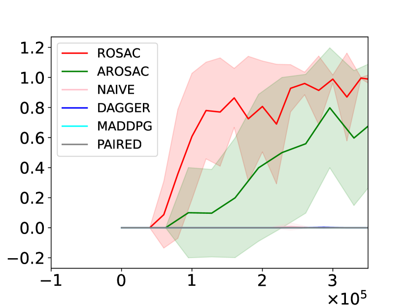
Refer to caption
(a) Success probability against
random adversary
Refer to caption
(b) Success probability against
Mcts adversary
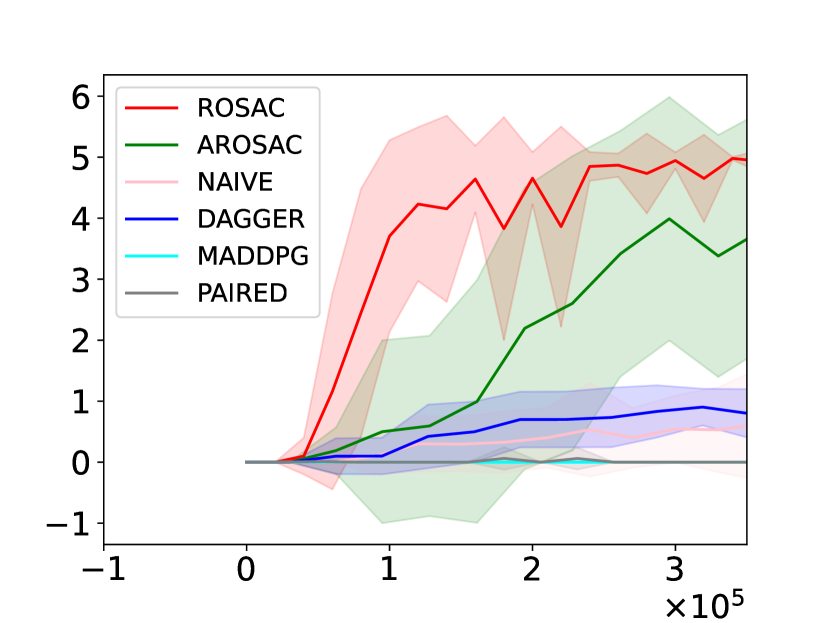
Refer to caption
(c) Number of subtasks completed against Mcts adversary
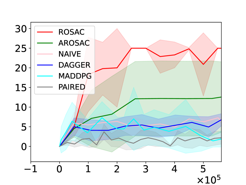
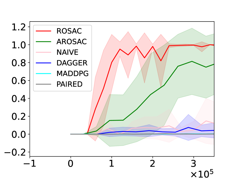
Figure 3: Plots for the Rooms environment. x𝑥x-axis denotes the number of sample steps and y𝑦y-axis denotes either the average number of subtasks completed or the probability of completing 5 subtasks. Results are averaged over 10 runs. Error bars indicate ±plus-or-minus\pm std.
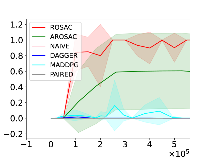
Refer to caption
(a) Success probability against
random adversary
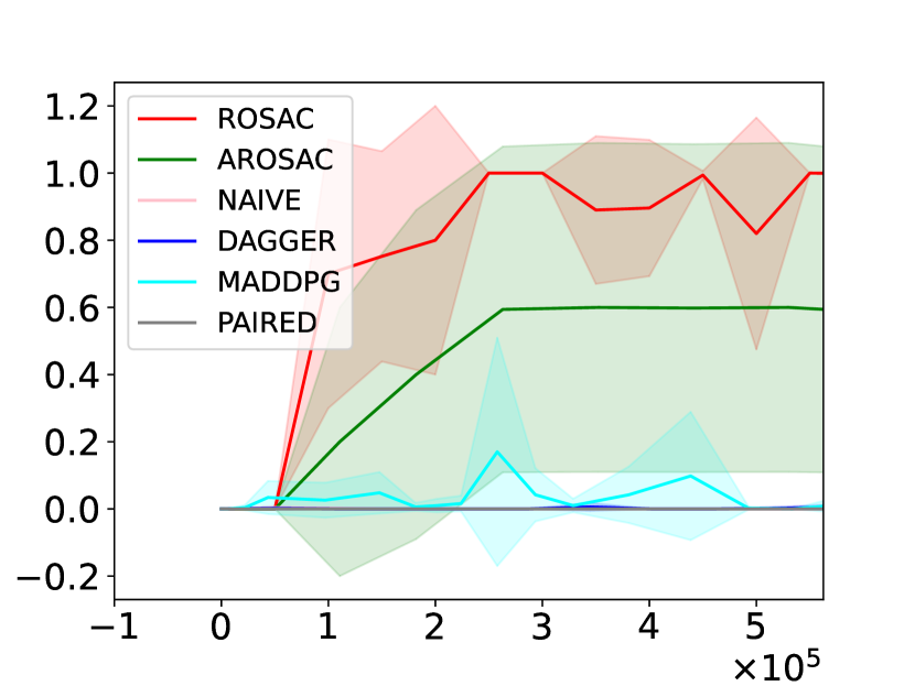
Refer to caption
(b) Success probability against
Mcts adversary
Refer to caption
(c) Number of subtasks completed against Mcts adversary
Figure 4: Plots for the F1/10th environment. x𝑥x-axis denotes the number of sample steps and y𝑦y-axis denotes either the average number of subtasks completed or the probability of completing 25 subtasks. Results are averaged over 5 runs. Error bars indicate ±plus-or-minus\pm std.

F1/10th environment.

This is the environment in the motivating example. A publicly available simulator (F, 110) of the F1/10th car is used for training and testing. The policies use the LiDAR measurements from the car as input (as opposed to the state) and we assume that the controller can detect the completion of each segment; as shown in prior work (Ivanov et al., 2021), one can train a separate neural network to predict subtask completion.

Baselines.

We compare our approach to four baselines. The baseline Naive trains one controller for each subtask with the only aim of completing the subtask, similar to the approach used by Ivanov et al. (2021), using a manually designed initial state distribution. Dagger is a similar approach which, instead of using a manually designed initial state distribution for training, infers the initial state distribution using the Dataset Aggregation principle (Ross et al., 2011). In other words, Dagger is similar to Arosac except that \mathcal{M} is used instead of σV~superscriptsubscript𝜎~𝑉\mathcal{M}_{\sigma}^{\tilde{V}} (Line 9 of Algorithm 3) for training the options in each iteration. The Maddpg baseline solves the game 𝒢𝒢\mathcal{G} using the multi-agent RL algorithm proposed by Lowe et al. (2017) for solving concurrent Markov games with continuous states and actions. We use the open-source implementation of Maddpg by the authors. The Paired baseline refers to the unsupervised environment design approach proposed by Dennis et al. (2020) in which the multi-task RL problem is viewed as a two-agent zero-sum game similar to our approach (but is not designed for long-horizon and compositional tasks). We implemented Paired with Ppo as the base algorithm to train the policies of the protagonist and the antagonist which consist of one NN policy per subtask. The adversary is parameterized by the probabilities (logits) of choosing various subtasks at different timesteps and is trained using Reinforce updates.

Refer to caption
(a) Success probability against
random adversary
Refer to caption
(b) Success probability against
Mcts adversary
Refer to caption
(c) Number of subtasks completed against Mcts adversary
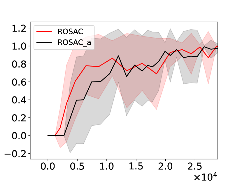
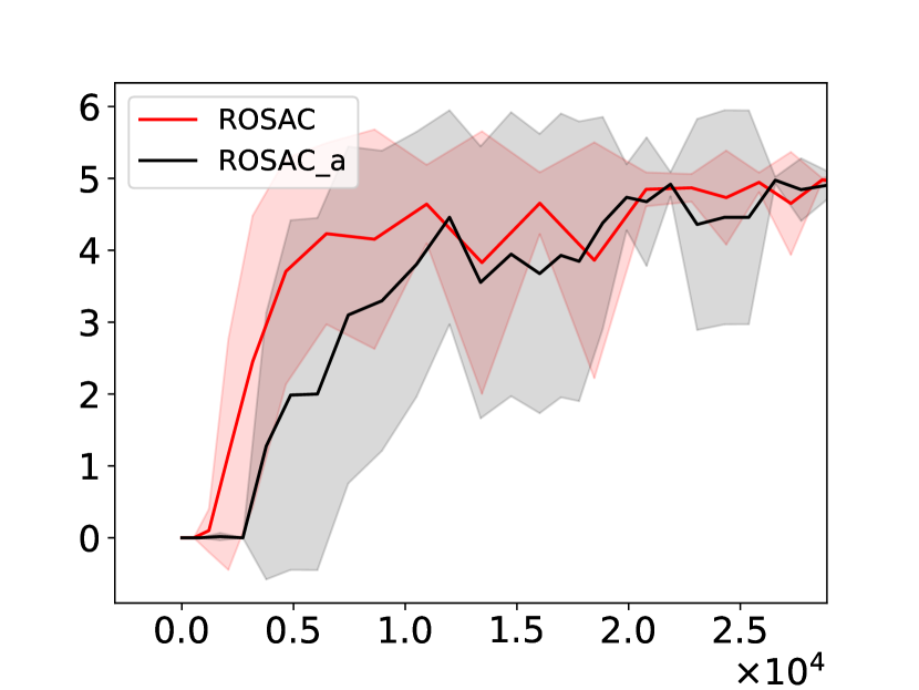
Figure 5: Ablation study in the Rooms environment. x𝑥x-axis denotes the number of sample steps and y𝑦y-axis denotes either the average number of subtasks completed or the probability of completing 5 subtasks. Results are averaged over 10 runs. Error bars indicate ±plus-or-minus\pm std.

Evaluation.

We evaluate the performance of these algorithms against two adversaries. One adversary is the random adversary which picks the next subtask uniformly at random from the set of all subtasks. The other adversary estimates the worst sequence of subtasks for a given set of options using Monte Carlo Tree Search algorithm (Mcts) (Kocsis and Szepesvári, 2006). The Mcts adversary is trained by assigning a reward of 111 if it selects a subtask which the corresponding policy is unable to complete within a fixed time budget and a reward of 00 otherwise. For the Rooms environment, we consider subtask sequences of length atmost 5 whereas for the F1/10th environment, we consider sequences of subtasks of length at most 25. We evaluate both the average number of subtasks completed as well as the probability of completing the set maximum number of subtasks.

Results.

The plots for the rooms environment are shown in Figure 3 and plots for the F1/10th environment are shown in Figure 4. We can observe that Rosac and Arosac outperform other approaches and learn robust options. Arosac performs worse as compared to Rosac; however, it has the added benefit of being parallelizable. Dagger and Naive baselines are unable to learn policies that can be used to perform long sequences of subtasks; this is mostly due to the fact that they learn options that cause the system to reach states from which future subtasks are difficult to perform—e.g., in the rooms environment, the agent sometimes reaches the left half of the exits from where it is difficult to reach the right exit in the subsequent room. Although Maddpg uses the same reduction to two-player games as Rosac, it ignores all the structure in the game and treats it as a generic Markov game. As a result, it learns a separate NN policy for each player which leads to the issue of unstable training, primarily due to the non-stationary nature of the environment observed by either agent. As shown in the plots, this leads to poor performance when applied to the problem of learning robust options. Similarly, Paired is unable to learn good options and is likely due to two reasons. Firstly, it does not use a compositional or a hierarchical approach for training the options, which causes it to scale poorly to long-horizon tasks. Secondly, it relies on “on policy” algorithms (such as Ppo) for training which are less efficient than Sac for our environments.

Random vs MCTS adversary.

Given that the number of subtasks is small in our benchmarks, the random adversary is able to select difficult sequences of subtasks often (eg., a right after a left in the Rooms environment), which explains the similarity in the observed performance against the two different adversaries. Nonetheless, even when the performance is measured against a random adversary, our approach significantly outperforms all baselines. An ablation study in the Rooms environment shows that selecting subtasks randomly during training is not as effective as the ε𝜀\varepsilon-greedy approach. In Figure 5, Rosaca denotes the ablation in which ε𝜀\varepsilon is set to 111 in line 14 of Algorithm 2. As the plots show, although this ablation is able to learn good subtask policies, it requires more samples than Rosac. Note that the ablation still uses the worst-case target value estimate over future subtasks V~~𝑉\tilde{V} for training the Q-networks.

6 Related Work

Options and Hierarchical RL.

The options framework (Sutton et al., 1999) is commonly used to model subtask policies as temporally extended actions. In hierarchical RL (Nachum et al., 2018, 2019; Kulkarni et al., 2016; Dietterich, 2000; Bacon et al., 2017; Tiwari and Thomas, 2019), options are trained along with a high-level controller that chooses the sequence of options (plan) to execute in order to complete a specific high-level task. In contrast, our approach aims to train options that work for multiple high-level plans. There is also work on discovering options—e.g., using intrinsic motivation (Machado et al., 2017), entropy maximization (Eysenbach et al., 2018), semi-supervised RL (Finn et al., 2017), skill chaining (Konidaris and Barto, 2009; Bagaria and Konidaris, 2019; Bagaria et al., 2021a), expectation maximization (Daniel et al., 2016) and subgoal identification (Stolle and Precup, 2002). Our approach is complementary to option discovery methods since our algorithm can be used to learn robust policies corresponding to the options which can be used in multiple contexts. There has also been a lot of research on planning using learned options (Abel et al., 2020; Jothimurugan et al., 2021; Precup et al., 1998; Theocharous and Kaelbling, 2004; Konidaris et al., 2014). Some hierarchical RL algorithms have also been shown to enable few-shot generalization (Jothimurugan et al., 2021) to unseen tasks. Closely related to our work is the work on compositional RL in the multi-task setting (Ivanov et al., 2021) in which the subtask policies are trained using standard RL algorithms in a naive way without guarantees regarding worst-case performance.

Multi-task RL.

There has been some work on RL for zero-shot generalization (Vaezipoor et al., 2021; Oh et al., 2017; Sohn et al., 2018; Kuo et al., 2020; Andreas et al., 2017); however, in these works, the learning objective is to maximize average performance with respect to a fixed distribution over tasks as opposed to the worst-case. Most closely related to our work is the line of work on minimax/robust RL (Pinto et al., 2017; Campero et al., 2020; Dennis et al., 2020), which aims to train policies to maximize the worst-case performance across multiple tasks/environments. However, there are a few key differences between existing work and our approach. Firstly, existing methods train a single NN policy to perform multiple tasks as opposed to training composable options for subtasks. As shown in the experiments, training a single policy does not scale well to complex long-horizon tasks. Secondly, these approaches do not provide strong convergence guarantees whereas we provide convergence guarantees in the finite-state setting. Finally, we utilize the structure in the problem to infer an adversary directly from the value functions instead of training a separate adversary as done in previous approaches.

Skill Chaining.

Research on skill chaining (Bagaria and Konidaris, 2019; Bagaria et al., 2021b, a; Lee et al., 2021) has led to algorithms for discovering and training options so that they compose well. However, in these approaches, the aim is to compose the options to perform a specific task which corresponds to executing the options in specific order(s). In contrast, our objective is independent of specific tasks and seeks to maximize performace across all tasks. Also, such approaches, at best, only provide hierarchical optimality guarantees whereas our algorithm converges to the optimal policy with respect to our game formulation. There has also been work on skill composition using transition policies (Lee et al., 2018); this method assumes that the subtask policies are fixed and learns one transition policy per subtask which takes the system from an end state to a “favourable” initial state for the subtask. However, poorly trained subtask policies can lead to situations in which it is not possible to achieve such transitions. In contrast, our approach trains subtask policies which compose well without requiring additional transition policies.

Multi-agent RL.

There has been a lot of research on multi-agent RL algorithms (Lowe et al., 2017; Hu and Wellman, 2003; Hu et al., 1998; Littman, 2001; Perolat et al., 2017; Prasad et al., 2015; Akchurina, 2008) including algorithms for two-agent zero-sum games (Bai and Jin, 2020; Wei et al., 2017; Littman, 1994). In this paper, we utilize the specific structure of our game to obtain a simple algorithm that neither requires solving matrix games nor trains a separate policy for the adversary. Furthermore, we show that we can obtain an asynchronous RL algorithm which enables training options in parallel.

7 Conclusions

We have proposed a framework for training robust options which can be used to perform arbitrary sequences of subtasks. We first reduce the problem to a two-agent zero-sum stagewise Markov game which has a unique structure. We utilized this structure to design two algorithms, namely Rosac and Arosac, and demonstrated that they outperform existing approaches for training options with respect to multi-task performance. One potential limitation of our approach is that the set of subtasks is fixed and has to be provided by the user. An interesting direction for future work is to address this limitation by combining our approach with option discovery methods.

Acknowledgements.

We thank the anonymous reviewers for their helpful comments. This research was partially supported by ONR award N00014-20-1-2115.

References

  • Abel et al. (2020) David Abel, Nathan Umbanhowar, Khimya Khetarpal, Dilip Arumugam, Doina Precup, and Michael L. Littman. Value preserving state-action abstractions. In Proceedings of the International Conference on Artificial Intelligence and Statistics, 2020.
  • Akchurina (2008) Natalia Akchurina. Multi-agent reinforcement learning algorithm with variable optimistic-pessimistic criterion. In ECAI, volume 178, pages 433–437, 2008.
  • Akkaya et al. (2019) Ilge Akkaya, Marcin Andrychowicz, Maciek Chociej, Mateusz Litwin, Bob McGrew, Arthur Petron, Alex Paino, Matthias Plappert, Glenn Powell, Raphael Ribas, et al. Solving rubik’s cube with a robot hand. arXiv preprint arXiv:1910.07113, 2019.
  • Andreas et al. (2017) Jacob Andreas, Dan Klein, and Sergey Levine. Modular multitask reinforcement learning with policy sketches. In International Conference on Machine Learning, pages 166–175. PMLR, 2017.
  • Bacon et al. (2017) Pierre-Luc Bacon, Jean Harb, and Doina Precup. The option-critic architecture. In Thirty-First AAAI Conference on Artificial Intelligence, 2017.
  • Bagaria and Konidaris (2019) Akhil Bagaria and George Konidaris. Option discovery using deep skill chaining. In International Conference on Learning Representations, 2019.
  • Bagaria et al. (2021a) Akhil Bagaria, Jason K Senthil, and George Konidaris. Skill discovery for exploration and planning using deep skill graphs. In International Conference on Machine Learning, pages 521–531. PMLR, 2021a.
  • Bagaria et al. (2021b) Akhil Bagaria, Jason K Senthil, Matthew Slivinski, and George Konidaris. Robustly learning composable options in deep reinforcement learning. In IJCAI, pages 2161–2169, 2021b.
  • Bai and Jin (2020) Yu Bai and Chi Jin. Provable self-play algorithms for competitive reinforcement learning. In Proceedings of the 37th International Conference on Machine Learning, 2020.
  • Bertsekas and Tsitsiklis (1996) D. P. Bertsekas and J. N. Tsitsiklis. Neuro-dynamic programming. Athena Scientific, Belmont, MA, 1996.
  • Campero et al. (2020) Andres Campero, Roberta Raileanu, Heinrich Küttler, Joshua B Tenenbaum, Tim Rocktäschel, and Edward Grefenstette. Learning with amigo: Adversarially motivated intrinsic goals. arXiv preprint arXiv:2006.12122, 2020.
  • Daniel et al. (2016) Christian Daniel, Herke Van Hoof, Jan Peters, and Gerhard Neumann. Probabilistic inference for determining options in reinforcement learning. Machine Learning, 104(2):337–357, 2016.
  • Dennis et al. (2020) Michael Dennis, Natasha Jaques, Eugene Vinitsky, Alexandre Bayen, Stuart Russell, Andrew Critch, and Sergey Levine. Emergent complexity and zero-shot transfer via unsupervised environment design. Advances in neural information processing systems, 33:13049–13061, 2020.
  • Dietterich (2000) Thomas G Dietterich. State abstraction in maxq hierarchical reinforcement learning. In Advances in Neural Information Processing Systems, pages 994–1000, 2000.
  • Eysenbach et al. (2018) Benjamin Eysenbach, Abhishek Gupta, Julian Ibarz, and Sergey Levine. Diversity is all you need: Learning skills without a reward function. In ICLR, 2018.
  • F (110) F110. F1/10 Autonomous Racing Competition. http://f1tenth.org.
  • Finn et al. (2017) Chelsea Finn, Tianhe Yu, Justin Fu, Pieter Abbeel, and Sergey Levine. Generalizing skills with semi-supervised reinforcement learning. In ICLR, 2017.
  • Fujimoto et al. (2018) Scott Fujimoto, Herke Hoof, and David Meger. Addressing function approximation error in actor-critic methods. In International Conference on Machine Learning, pages 1587–1596, 2018.
  • Haarnoja et al. (2018) Tuomas Haarnoja, Aurick Zhou, Pieter Abbeel, and Sergey Levine. Soft actor-critic: Off-policy maximum entropy deep reinforcement learning with a stochastic actor. In International conference on machine learning, pages 1861–1870. PMLR, 2018.
  • Hu and Wellman (2003) Junling Hu and Michael P Wellman. Nash q-learning for general-sum stochastic games. Journal of machine learning research, 4(Nov):1039–1069, 2003.
  • Hu et al. (1998) Junling Hu, Michael P Wellman, et al. Multiagent reinforcement learning: theoretical framework and an algorithm. In ICML, volume 98, pages 242–250. Citeseer, 1998.
  • Ivanov et al. (2021) Radoslav Ivanov, Kishor Jothimurugan, Steve Hsu, Shaan Vaidya, Rajeev Alur, and Osbert Bastani. Compositional learning and verification of neural network controllers. ACM Transactions on Embedded Computing Systems (TECS), 20(5s):1–26, 2021.
  • Jothimurugan et al. (2021) Kishor Jothimurugan, Osbert Bastani, and Rajeev Alur. Abstract value iteration for hierarchical reinforcement learning. In Arindam Banerjee and Kenji Fukumizu, editors, Proceedings of The 24th International Conference on Artificial Intelligence and Statistics, volume 130 of Proceedings of Machine Learning Research, pages 1162–1170. PMLR, 13–15 Apr 2021.
  • Kocsis and Szepesvári (2006) Levente Kocsis and Csaba Szepesvári. Bandit based monte-carlo planning. In European conference on machine learning, pages 282–293. Springer, 2006.
  • Konidaris and Barto (2009) George Konidaris and Andrew G Barto. Skill discovery in continuous reinforcement learning domains using skill chaining. In Advances in neural information processing systems, pages 1015–1023, 2009.
  • Konidaris et al. (2014) George Konidaris, Leslie Kaelbling, and Tomas Lozano-Perez. Constructing symbolic representations for high-level planning. In Twenty-Eighth AAAI Conference on Artificial Intelligence, 2014.
  • Kulkarni et al. (2016) Tejas D Kulkarni, Karthik Narasimhan, Ardavan Saeedi, and Josh Tenenbaum. Hierarchical deep reinforcement learning: Integrating temporal abstraction and intrinsic motivation. In Advances in neural information processing systems, pages 3675–3683, 2016.
  • Kuo et al. (2020) Yen-Ling Kuo, Boris Katz, and Andrei Barbu. Encoding formulas as deep networks: Reinforcement learning for zero-shot execution of ltl formulas. 2020 IEEE/RSJ International Conference on Intelligent Robots and Systems (IROS), pages 5604–5610, 2020.
  • Lee et al. (2018) Youngwoon Lee, Shao-Hua Sun, Sriram Somasundaram, Edward S Hu, and Joseph J Lim. Composing complex skills by learning transition policies. In International Conference on Learning Representations, 2018.
  • Lee et al. (2021) Youngwoon Lee, Joseph J Lim, Anima Anandkumar, and Yuke Zhu. Adversarial skill chaining for long-horizon robot manipulation via terminal state regularization. arXiv preprint arXiv:2111.07999, 2021.
  • Lillicrap et al. (2016) Timothy P Lillicrap, Jonathan J Hunt, Alexander Pritzel, Nicolas Heess, Tom Erez, Yuval Tassa, David Silver, and Daan Wierstra. Continuous control with deep reinforcement learning. In ICLR, 2016.
  • Littman (1994) Michael L Littman. Markov games as a framework for multi-agent reinforcement learning. In Machine learning proceedings 1994, pages 157–163. Elsevier, 1994.
  • Littman (2001) Michael L Littman. Friend-or-foe q-learning in general-sum games. In ICML, volume 1, pages 322–328, 2001.
  • Lowe et al. (2017) Ryan Lowe, Yi Wu, Aviv Tamar, Jean Harb, Pieter Abbeel, and Igor Mordatch. Multi-agent actor-critic for mixed cooperative-competitive environments. In Proceedings of the 31st International Conference on Neural Information Processing Systems, pages 6382–6393, 2017.
  • Machado et al. (2017) Marios C Machado, Marc G Bellemare, and Michael Bowling. A laplacian framework for option discovery in reinforcement learning. In Proceedings of the 34th International Conference on Machine Learning-Volume 70, pages 2295–2304. JMLR. org, 2017.
  • Nachum et al. (2018) Ofir Nachum, Shixiang Shane Gu, Honglak Lee, and Sergey Levine. Data-efficient hierarchical reinforcement learning. In Advances in Neural Information Processing Systems, pages 3303–3313, 2018.
  • Nachum et al. (2019) Ofir Nachum, Shixiang Gu, Honglak Lee, and Sergey Levine. Near-optimal representation learning for hierarchical reinforcement learning. In ICLR, 2019.
  • Oh et al. (2017) Junhyuk Oh, Satinder Singh, Honglak Lee, and Pushmeet Kohli. Zero-shot task generalization with multi-task deep reinforcement learning. In International Conference on Machine Learning, pages 2661–2670. PMLR, 2017.
  • Patek (1997) Stephen David Patek. Stochastic and shortest path games: theory and algorithms. PhD thesis, Massachusetts Institute of Technology, 1997.
  • Perolat et al. (2017) Julien Perolat, Florian Strub, Bilal Piot, and Olivier Pietquin. Learning Nash Equilibrium for General-Sum Markov Games from Batch Data. In Proceedings of the 20th International Conference on Artificial Intelligence and Statistics, 2017.
  • Pinto et al. (2017) Lerrel Pinto, James Davidson, Rahul Sukthankar, and Abhinav Gupta. Robust adversarial reinforcement learning. In International Conference on Machine Learning, pages 2817–2826. PMLR, 2017.
  • Prasad et al. (2015) HL Prasad, Prashanth LA, and Shalabh Bhatnagar. Two-timescale algorithms for learning nash equilibria in general-sum stochastic games. In Proceedings of the 2015 International Conference on Autonomous Agents and Multiagent Systems, pages 1371–1379, 2015.
  • Precup et al. (1998) Doina Precup, Richard S Sutton, and Satinder Singh. Theoretical results on reinforcement learning with temporally abstract options. In European conference on machine learning, pages 382–393. Springer, 1998.
  • Ross et al. (2011) Stéphane Ross, Geoffrey Gordon, and Drew Bagnell. A reduction of imitation learning and structured prediction to no-regret online learning. In Proceedings of the fourteenth international conference on artificial intelligence and statistics, pages 627–635, 2011.
  • Sohn et al. (2018) Sungryull Sohn, Junhyuk Oh, and Honglak Lee. Hierarchical reinforcement learning for zero-shot generalization with subtask dependencies. Advances in Neural Information Processing Systems, 31, 2018.
  • Stolle and Precup (2002) Martin Stolle and Doina Precup. Learning options in reinforcement learning. In International Symposium on abstraction, reformulation, and approximation, pages 212–223. Springer, 2002.
  • Sutton et al. (1999) Richard S Sutton, Doina Precup, and Satinder Singh. Between mdps and semi-mdps: A framework for temporal abstraction in reinforcement learning. Artificial intelligence, 112(1-2):181–211, 1999.
  • Theocharous and Kaelbling (2004) Georgios Theocharous and Leslie P Kaelbling. Approximate planning in pomdps with macro-actions. In Advances in Neural Information Processing Systems, pages 775–782, 2004.
  • Tiwari and Thomas (2019) Saket Tiwari and Philip S Thomas. Natural option critic. In Proceedings of the AAAI Conference on Artificial Intelligence, volume 33, pages 5175–5182, 2019.
  • Vaezipoor et al. (2021) Pashootan Vaezipoor, Andrew C Li, Rodrigo A Toro Icarte, and Sheila A. Mcilraith. Ltl2action: Generalizing ltl instructions for multi-task rl. In Marina Meila and Tong Zhang, editors, Proceedings of the 38th International Conference on Machine Learning, volume 139 of Proceedings of Machine Learning Research, pages 10497–10508. PMLR, 18–24 Jul 2021.
  • Wei et al. (2017) Chen-Yu Wei, Yi-Te Hong, and Chi-Jen Lu. Online reinforcement learning in stochastic games. In Proceedings of the 31st International Conference on Neural Information Processing Systems, pages 4994–5004, 2017.

Appendix A Proofs

In this section, we prove the theorems presented in the paper through a series of lemmas. The proofs here are adaptations of proofs of similar results for zero-sum concurrent games with a single discount factor [Patek, 1997].

A.1 Definitions

We first introduce some notation and definitions. Recall that we defined S1={(s,σ)σFσ}subscript𝑆1conditional-set𝑠𝜎𝜎subscript𝐹𝜎S_{1}=\{(s,\sigma)\mid\sigma\notin F_{\sigma}\}, S2={(s,σ)σFσ}subscript𝑆2conditional-set𝑠𝜎𝜎subscript𝐹𝜎S_{2}=\{(s,\sigma)\mid\sigma\in F_{\sigma}\} and S¯=S1S2¯𝑆subscript𝑆1subscript𝑆2\bar{S}=S_{1}\cup S_{2}. 𝒱={V:S1}𝒱conditional-set𝑉subscript𝑆1\mathcal{V}=\{V:S_{1}\to\mathbb{R}\} denotes the set of value functions over S1subscript𝑆1S_{1} and 𝒱¯={V:S¯}¯𝒱conditional-set𝑉¯𝑆\bar{\mathcal{V}}=\{V:\bar{S}\to\mathbb{R}\} denotes the set of value functions over S¯¯𝑆\bar{S}. We use delimited-∥∥{\lVert\cdot\rVert} to denote the subscript\ell_{\infty}-norm. For any V𝒱𝑉𝒱V\in\mathcal{V}, (s,σ)S2𝑠𝜎subscript𝑆2(s,\sigma)\in S_{2} and any σΣsuperscript𝜎Σ\sigma^{\prime}\in\Sigma, define

Vσ(s,σ)=sSTσ(ss)V(s,σ).{\llbracket V\rrbracket}_{\sigma^{\prime}}(s,\sigma)=\sum_{s^{\prime}\in S}T_{\sigma}(s^{\prime}\mid s)V(s^{\prime},\sigma^{\prime}).

Note that for any (s,σ)S2𝑠𝜎subscript𝑆2(s,\sigma)\in S_{2}, we have V(s,σ)=minσΣVσ(s,σ){\llbracket V\rrbracket}(s,\sigma)=\min_{\sigma^{\prime}\in\Sigma}{\llbracket V\rrbracket}_{\sigma^{\prime}}(s,\sigma). Similarly, for any V𝒱𝑉𝒱V\in\mathcal{V}, (s,σ)S1𝑠𝜎subscript𝑆1(s,\sigma)\in S_{1} and aA𝑎𝐴a\in A, let us define

a(V)(s,σ)=R¯((s,σ),a)+γsSP(ss,a)V(s,σ)\mathcal{F}_{a}(V)(s,\sigma)=\bar{R}((s,\sigma),a)+\gamma\cdot\sum_{s^{\prime}\in S}P(s^{\prime}\mid s,a){\llbracket V\rrbracket}(s^{\prime},\sigma)

with (V)(s,σ)=maxaAa(V)(s,σ)𝑉𝑠𝜎subscript𝑎𝐴subscript𝑎𝑉𝑠𝜎\mathcal{F}(V)(s,\sigma)=\max_{a\in A}\mathcal{F}_{a}(V)(s,\sigma). Given any policy π1:S¯A1:subscript𝜋1¯𝑆subscript𝐴1\pi_{1}:\bar{S}\to A_{1} for agent 1 in 𝒢𝒢\mathcal{G}, we define the resulting MDP 𝒢(π1)=(S¯,A2,Pπ1,Rπ1,γ)𝒢subscript𝜋1¯𝑆subscript𝐴2subscript𝑃subscript𝜋1subscript𝑅subscript𝜋1𝛾\mathcal{G}(\pi_{1})=(\bar{S},A_{2},P_{\pi_{1}},R_{\pi_{1}},\gamma) with states S¯¯𝑆\bar{S} and actions 𝒜2=Σsubscript𝒜2Σ\mathcal{A}_{2}=\Sigma as follows. The transition probability function is given by

Pπ1((s,σ)(s,σ),a2)={P¯((s,σ)(s,σ),π1(s,σ),a2)if(s,σ)S1s′′STσ(s′′s)P¯((s,σ)(s′′,a2),π1(s′′,a2),a2)if(s,σ)S2subscript𝑃subscript𝜋1conditionalsuperscript𝑠superscript𝜎𝑠𝜎subscript𝑎2cases¯𝑃conditionalsuperscript𝑠superscript𝜎𝑠𝜎subscript𝜋1𝑠𝜎subscript𝑎2if𝑠𝜎subscript𝑆1subscriptsuperscript𝑠′′𝑆subscript𝑇𝜎conditionalsuperscript𝑠′′𝑠¯𝑃conditionalsuperscript𝑠superscript𝜎superscript𝑠′′subscript𝑎2subscript𝜋1superscript𝑠′′subscript𝑎2subscript𝑎2if𝑠𝜎subscript𝑆2P_{\pi_{1}}((s^{\prime},\sigma^{\prime})\mid(s,\sigma),a_{2})=\begin{cases}\bar{P}((s^{\prime},\sigma^{\prime})\mid(s,\sigma),\pi_{1}(s,\sigma),a_{2})&\text{if}\ (s,\sigma)\in S_{1}\\ \sum_{s^{\prime\prime}\in S}T_{\sigma}(s^{\prime\prime}\mid s)\bar{P}((s^{\prime},\sigma^{\prime})\mid(s^{\prime\prime},a_{2}),\pi_{1}(s^{\prime\prime},a_{2}),a_{2})&\text{if}\ (s,\sigma)\in S_{2}\end{cases}

and the reward function is given by

Rπ1((s,σ),a2)={R¯((s,σ),π1(s,σ))if(s,σ)S1sSTσ(ss)R¯((s,a2),π1(s,a2))if(s,σ)S2.subscript𝑅subscript𝜋1𝑠𝜎subscript𝑎2cases¯𝑅𝑠𝜎subscript𝜋1𝑠𝜎if𝑠𝜎subscript𝑆1subscriptsuperscript𝑠𝑆subscript𝑇𝜎conditionalsuperscript𝑠𝑠¯𝑅superscript𝑠subscript𝑎2subscript𝜋1superscript𝑠subscript𝑎2if𝑠𝜎subscript𝑆2R_{\pi_{1}}((s,\sigma),a_{2})=\begin{cases}-\bar{R}((s,\sigma),\pi_{1}(s,\sigma))&\text{if}\ (s,\sigma)\in S_{1}\\ -\sum_{s^{\prime}\in S}T_{\sigma}(s^{\prime}\mid s)\bar{R}((s^{\prime},a_{2}),\pi_{1}(s^{\prime},a_{2}))&\text{if}\ (s,\sigma)\in S_{2}.\end{cases}

Intuitively, the MDP 𝒢(π1)𝒢subscript𝜋1\mathcal{G}(\pi_{1}) merges every step of 𝒢𝒢\mathcal{G} in which a change of subtask occurs with the subsequent step in the environment, while using π1subscript𝜋1\pi_{1} to choose actions for agent 1. For any s¯S¯¯𝑠¯𝑆\bar{s}\in\bar{S}, let 𝒟s¯𝒢(π1)(π2)subscriptsuperscript𝒟𝒢subscript𝜋1¯𝑠subscript𝜋2\mathcal{D}^{\mathcal{G}(\pi_{1})}_{\bar{s}}(\pi_{2}) denote the distribution over infinite trajectories generated by π2subscript𝜋2\pi_{2} starting at s¯¯𝑠\bar{s} in 𝒢(π1)𝒢subscript𝜋1\mathcal{G}(\pi_{1}). Then we define the value function for the MDP 𝒢(π1)𝒢subscript𝜋1\mathcal{G}(\pi_{1}) using

V𝒢(π1)π2(s¯)=𝔼ρ𝒟s¯𝒢(π1)(π2)[t=0γtRπ1(s¯t,at)]superscriptsubscript𝑉𝒢subscript𝜋1subscript𝜋2¯𝑠subscript𝔼similar-to𝜌subscriptsuperscript𝒟𝒢subscript𝜋1¯𝑠subscript𝜋2delimited-[]superscriptsubscript𝑡0superscript𝛾𝑡subscript𝑅subscript𝜋1subscript¯𝑠𝑡subscript𝑎𝑡V_{\mathcal{G}(\pi_{1})}^{\pi_{2}}(\bar{s})=\mathbb{E}_{\rho\sim\mathcal{D}^{\mathcal{G}(\pi_{1})}_{\bar{s}}(\pi_{2})}\Big{[}\sum_{t=0}^{\infty}\gamma^{t}R_{\pi_{1}}(\bar{s}_{t},a_{t})\Big{]}

for all π2:S¯A2:subscript𝜋2¯𝑆subscript𝐴2\pi_{2}:\bar{S}\to A_{2} and s¯S¯¯𝑠¯𝑆\bar{s}\in\bar{S}.

A.2 Necessary Lemmas

We need a few intermediate results in order to prove the main theorems. We begin by analyzing the operators :𝒱𝒱¯{\llbracket\cdot\rrbracket}:\mathcal{V}\to\bar{\mathcal{V}} and :𝒱𝒱:𝒱𝒱\mathcal{F}:\mathcal{V}\to\mathcal{V} defined in Section 3.1.

Lemma A.1.

For any V1,V2𝒱subscript𝑉1subscript𝑉2𝒱V_{1},V_{2}\in\mathcal{V}, we have V1V2=V1V2{\lVert{\llbracket V_{1}\rrbracket}-{\llbracket V_{2}\rrbracket}\rVert}={\lVert V_{1}-V_{2}\rVert}.

Proof.

For any (s,σ)S1𝑠𝜎subscript𝑆1(s,\sigma)\in S_{1}, we have |V1(s,σ)V2(s,σ)|=|V1(s,σ)V2(s,σ)|{\lvert{\llbracket V_{1}\rrbracket}(s,\sigma)-{\llbracket V_{2}\rrbracket}(s,\sigma)\rvert}={\lvert V_{1}(s,\sigma)-V_{2}(s,\sigma)\rvert}. For any (s,σ)S2𝑠𝜎subscript𝑆2(s,\sigma)\in S_{2} and σΣsuperscript𝜎Σ\sigma^{\prime}\in\Sigma we have

|V1σ(s,σ)V2σ(s,σ)|\displaystyle{\lvert{\llbracket V_{1}\rrbracket}_{\sigma^{\prime}}(s,\sigma)-{\llbracket V_{2}\rrbracket}_{\sigma^{\prime}}(s,\sigma)\rvert} =sSTσ(ss)V1(s,σ)sSTσ(ss)V2(s,σ)absentdelimited-∥∥subscriptsuperscript𝑠𝑆subscript𝑇𝜎conditionalsuperscript𝑠𝑠subscript𝑉1superscript𝑠superscript𝜎subscriptsuperscript𝑠𝑆subscript𝑇𝜎conditionalsuperscript𝑠𝑠subscript𝑉2superscript𝑠superscript𝜎\displaystyle={\lVert\sum_{s^{\prime}\in S}T_{\sigma}(s^{\prime}\mid s)V_{1}(s^{\prime},\sigma^{\prime})-\sum_{s^{\prime}\in S}T_{\sigma}(s^{\prime}\mid s)V_{2}(s^{\prime},\sigma^{\prime})\rVert}
sSTσ(ss)|V1(s,σ)V2(s,σ)|absentsubscriptsuperscript𝑠𝑆subscript𝑇𝜎conditionalsuperscript𝑠𝑠subscript𝑉1superscript𝑠superscript𝜎subscript𝑉2superscript𝑠superscript𝜎\displaystyle\leq\sum_{s^{\prime}\in S}T_{\sigma}(s^{\prime}\mid s){\lvert V_{1}(s^{\prime},\sigma^{\prime})-V_{2}(s^{\prime},\sigma^{\prime})\rvert}
V1V2.absentdelimited-∥∥subscript𝑉1subscript𝑉2\displaystyle\leq{\lVert V_{1}-V_{2}\rVert}.

Now we have |V1(s,σ)V2(s,σ)|=|minσV1σ(s,σ)minσV2σ(s,σ)|V1V2{\lvert{\llbracket V_{1}\rrbracket}(s,\sigma)-{\llbracket V_{2}\rrbracket}(s,\sigma)\rvert}={\lvert\min_{\sigma^{\prime}}{\llbracket V_{1}\rrbracket}_{\sigma^{\prime}}(s,\sigma)-\min_{\sigma^{\prime}}{\llbracket V_{2}\rrbracket}_{\sigma^{\prime}}(s,\sigma)\rvert}\leq{\lVert V_{1}-V_{2}\rVert} which concludes the proof. ∎

Now we are ready to show that \mathcal{F} is a contraction.

Lemma A.2.

:𝒱𝒱:𝒱𝒱\mathcal{F}:\mathcal{V}\to\mathcal{V} is a contraction mapping w.r.t the norm delimited-∥∥{\lVert\cdot\rVert}.

Proof.

Let V1,V2𝒱subscript𝑉1subscript𝑉2𝒱V_{1},V_{2}\in\mathcal{V}. Then for any (s,σ)S1𝑠𝜎subscript𝑆1(s,\sigma)\in S_{1} and aA𝑎𝐴a\in A,

|a(V1)(s,σ)a(V2)(s,σ)|subscript𝑎subscript𝑉1𝑠𝜎subscript𝑎subscript𝑉2𝑠𝜎\displaystyle{\lvert\mathcal{F}_{a}(V_{1})(s,\sigma)-\mathcal{F}_{a}(V_{2})(s,\sigma)\rvert} =|γsSP(ss,a)V1(s,σ)γsSP(ss,a)V2(s,σ)|\displaystyle={\lvert\gamma\sum_{s^{\prime}\in S}P(s^{\prime}\mid s,a){\llbracket V_{1}\rrbracket}(s^{\prime},\sigma)-\gamma\sum_{s^{\prime}\in S}P(s^{\prime}\mid s,a){\llbracket V_{2}\rrbracket}(s^{\prime},\sigma)\rvert}
γsSP(ss,a)|V1(s,σ)V2(s,σ)|\displaystyle\leq\gamma\sum_{s^{\prime}\in S}P(s^{\prime}\mid s,a){\lvert{\llbracket V_{1}\rrbracket}(s^{\prime},\sigma)-{\llbracket V_{2}\rrbracket}(s^{\prime},\sigma)\rvert}
γV1V2absent𝛾delimited-∥∥subscript𝑉1subscript𝑉2\displaystyle\leq\gamma{\lVert V_{1}-V_{2}\rVert}

where the last inequality followed from Lemma A.1. Therefore, for any (s,σ)S1𝑠𝜎subscript𝑆1(s,\sigma)\in S_{1}, we have |(V1)(s,σ)(V2)(s,σ)|=|maxaa(V1)(s,σ)maxaa(V2)(s,σ)|γV1V2subscript𝑉1𝑠𝜎subscript𝑉2𝑠𝜎subscript𝑎subscript𝑎subscript𝑉1𝑠𝜎subscript𝑎subscript𝑎subscript𝑉2𝑠𝜎𝛾delimited-∥∥subscript𝑉1subscript𝑉2{\lvert\mathcal{F}(V_{1})(s,\sigma)-\mathcal{F}(V_{2})(s,\sigma)\rvert}={\lvert\max_{a}\mathcal{F}_{a}(V_{1})(s,\sigma)-\max_{a}\mathcal{F}_{a}(V_{2})(s,\sigma)\rvert}\leq\gamma{\lVert V_{1}-V_{2}\rVert} showing that \mathcal{F} is a contraction. ∎

Now we connect the value function of the game 𝒢𝒢\mathcal{G} with that of the MDP 𝒢(π1)𝒢subscript𝜋1\mathcal{G}(\pi_{1}).

Lemma A.3.

For any π1:S¯A1:subscript𝜋1¯𝑆subscript𝐴1\pi_{1}:\bar{S}\to A_{1}, π2:S¯A2:subscript𝜋2¯𝑆subscript𝐴2\pi_{2}:\bar{S}\to A_{2} and s¯S¯¯𝑠¯𝑆\bar{s}\in\bar{S}, Vπ1,π2(s¯)=V𝒢(π1)π2(s¯)superscript𝑉subscript𝜋1subscript𝜋2¯𝑠superscriptsubscript𝑉𝒢subscript𝜋1subscript𝜋2¯𝑠V^{\pi_{1},\pi_{2}}(\bar{s})=-V_{\mathcal{G}(\pi_{1})}^{\pi_{2}}(\bar{s}).

Proof.

Given an infinite trajectory ρ¯=s¯0a01a02s¯1a11a12¯𝜌subscript¯𝑠0superscriptsubscript𝑎01superscriptsubscript𝑎02subscript¯𝑠1superscriptsubscript𝑎11superscriptsubscript𝑎12\bar{\rho}=\bar{s}_{0}a_{0}^{1}a_{0}^{2}\bar{s}_{1}a_{1}^{1}a_{1}^{2}\ldots in 𝒢𝒢\mathcal{G} we define a corresponding trajectory ρ¯2=s¯i0ai02s¯i1ai12subscript¯𝜌2subscript¯𝑠subscript𝑖0superscriptsubscript𝑎subscript𝑖02subscript¯𝑠subscript𝑖1superscriptsubscript𝑎subscript𝑖12\bar{\rho}_{2}=\bar{s}_{i_{0}}a_{i_{0}}^{2}\bar{s}_{i_{1}}a_{i_{1}}^{2} in 𝒢(π1)𝒢subscript𝜋1\mathcal{G}(\pi_{1}) as a subsequence where i0=0subscript𝑖00i_{0}=0 and it+1=it+1subscript𝑖𝑡1subscript𝑖𝑡1i_{t+1}=i_{t}+1 if s¯itS1subscript¯𝑠subscript𝑖𝑡subscript𝑆1\bar{s}_{i_{t}}\in S_{1} and it+1=it+2subscript𝑖𝑡1subscript𝑖𝑡2i_{t+1}=i_{t}+2 if s¯itS2subscript¯𝑠subscript𝑖𝑡subscript𝑆2\bar{s}_{i_{t}}\in S_{2}. Then for any s¯S¯¯𝑠¯𝑆\bar{s}\in\bar{S} we have

Vπ1,π2(s¯)superscript𝑉subscript𝜋1subscript𝜋2¯𝑠\displaystyle V^{\pi_{1},\pi_{2}}(\bar{s}) =𝔼ρ¯𝒟s¯𝒢(π1,π2)[t=0(k=0t1γ¯(s¯k))R¯(s¯t,at1)]absentsubscript𝔼similar-to¯𝜌subscriptsuperscript𝒟𝒢¯𝑠subscript𝜋1subscript𝜋2delimited-[]superscriptsubscript𝑡0superscriptsubscriptproduct𝑘0𝑡1¯𝛾subscript¯𝑠𝑘¯𝑅subscript¯𝑠𝑡superscriptsubscript𝑎𝑡1\displaystyle=\mathbb{E}_{\bar{\rho}\sim\mathcal{D}^{\mathcal{G}}_{\bar{s}}({\pi}_{1},{\pi}_{2})}\Big{[}\sum_{t=0}^{\infty}\big{(}\prod_{k=0}^{t-1}\bar{\gamma}(\bar{s}_{k})\big{)}\bar{R}(\bar{s}_{t},a_{t}^{1})\Big{]}
=(1)𝔼ρ¯𝒟s¯𝒢(π1,π2)[t=0γtRπ1(s¯it,ait2)]superscript1absentsubscript𝔼similar-to¯𝜌subscriptsuperscript𝒟𝒢¯𝑠subscript𝜋1subscript𝜋2delimited-[]superscriptsubscript𝑡0superscript𝛾𝑡subscript𝑅subscript𝜋1subscript¯𝑠subscript𝑖𝑡superscriptsubscript𝑎subscript𝑖𝑡2\displaystyle\stackrel{{\scriptstyle(1)}}{{=}}\mathbb{E}_{\bar{\rho}\sim\mathcal{D}^{\mathcal{G}}_{\bar{s}}({\pi}_{1},{\pi}_{2})}\Big{[}\sum_{t=0}^{\infty}\gamma^{t}{R}_{\pi_{1}}(\bar{s}_{i_{t}},a_{i_{t}}^{2})\Big{]}
=(2)𝔼ρ𝒟s¯𝒢(π1)(π2)[t=0γtRπ1(s¯t,at)]superscript2absentsubscript𝔼similar-to𝜌subscriptsuperscript𝒟𝒢subscript𝜋1¯𝑠subscript𝜋2delimited-[]superscriptsubscript𝑡0superscript𝛾𝑡subscript𝑅subscript𝜋1subscript¯𝑠𝑡subscript𝑎𝑡\displaystyle\stackrel{{\scriptstyle(2)}}{{=}}-\mathbb{E}_{{\rho}\sim\mathcal{D}^{\mathcal{G}(\pi_{1})}_{\bar{s}}({\pi}_{2})}\Big{[}\sum_{t=0}^{\infty}\gamma^{t}{R}_{\pi_{1}}(\bar{s}_{t},a_{t})\Big{]}
=V𝒢(π1)π2(s¯)absentsuperscriptsubscript𝑉𝒢subscript𝜋1subscript𝜋2¯𝑠\displaystyle=-V_{\mathcal{G}(\pi_{1})}^{\pi_{2}}(\bar{s})

where (1) followed from the definitions of γ¯¯𝛾\bar{\gamma} and Rπ1subscript𝑅subscript𝜋1R_{\pi_{1}} and the fact that R¯(s¯t,at1)=0¯𝑅subscript¯𝑠𝑡superscriptsubscript𝑎𝑡10\bar{R}(\bar{s}_{t},a_{t}^{1})=0 if s¯tS2subscript¯𝑠𝑡subscript𝑆2\bar{s}_{t}\in S_{2}, and (2) followed from the fact that sampling a trajectory ρ𝜌{\rho} by first sampling ρ¯¯𝜌\bar{\rho} from 𝒟s¯𝒢(π1,π2)subscriptsuperscript𝒟𝒢¯𝑠subscript𝜋1subscript𝜋2\mathcal{D}^{\mathcal{G}}_{\bar{s}}({\pi}_{1},{\pi}_{2}) and then constructing the subsequence ρ¯2subscript¯𝜌2\bar{\rho}_{2} is the same as sampling an infinite trajectory ρ𝜌{\rho} from 𝒟s¯𝒢(π1)(π2)subscriptsuperscript𝒟𝒢subscript𝜋1¯𝑠subscript𝜋2\mathcal{D}^{\mathcal{G}(\pi_{1})}_{\bar{s}}({\pi}_{2})888This can be shown formally by analyzing the probabilities assigned by the two distributions on cylinder sets.. ∎

Lemma A.2 shows that for any V𝒱𝑉𝒱V\in\mathcal{V} we have

limnn(V)=Vlimsubscript𝑛superscript𝑛𝑉subscript𝑉\lim_{n\to\infty}\mathcal{F}^{n}(V)=V_{\lim}

where Vlim𝒱subscript𝑉𝒱V_{\lim}\in\mathcal{V} is the unique fixed point of \mathcal{F}. Now we define two policies π1superscriptsubscript𝜋1\pi_{1}^{*} and π2superscriptsubscript𝜋2\pi_{2}^{*} for agents 1 and 2 respectively, as follows. For (s,σ)S1𝑠𝜎subscript𝑆1(s,\sigma)\in S_{1} we have

π1(s,σ)argmaxaAa(Vlim)(s,σ)superscriptsubscript𝜋1𝑠𝜎subscript𝑎𝐴subscript𝑎subscript𝑉𝑠𝜎\pi_{1}^{*}(s,\sigma)\in\operatorname{\arg\max}_{a\in A}\mathcal{F}_{a}(V_{\lim})(s,\sigma) (4)

and for (s,σ)S2𝑠𝜎subscript𝑆2(s,\sigma)\in S_{2}, we have

π2(s,σ)argminσVlimσ(s,σ).\pi^{*}_{2}(s,\sigma)\in\operatorname{\arg\min}_{\sigma^{\prime}}{\llbracket V_{\lim}\rrbracket}_{\sigma^{\prime}}(s,\sigma). (5)

Note that the actions taken by π1superscriptsubscript𝜋1\pi_{1}^{*} in S2subscript𝑆2S_{2} and π2superscriptsubscript𝜋2\pi_{2}^{*} in S1subscript𝑆1S_{1} can be arbitrary since they do not affect the transitions of the game 𝒢𝒢\mathcal{G}. Now we show that for any s¯S¯¯𝑠¯𝑆\bar{s}\in\bar{S}, π1subscriptsuperscript𝜋1\pi^{*}_{1} maximizes Vπ1,π2(s¯)superscript𝑉subscript𝜋1superscriptsubscript𝜋2¯𝑠V^{\pi_{1},\pi_{2}^{*}}(\bar{s}) and π2subscriptsuperscript𝜋2\pi^{*}_{2} minimizes Vπ1,π2(s¯)superscript𝑉subscriptsuperscript𝜋1subscript𝜋2¯𝑠V^{{\pi}^{*}_{1},{\pi}_{2}}(\bar{s}).

Lemma A.4.

For any s¯S¯¯𝑠¯𝑆\bar{s}\in\bar{S}, Vπ1,π2(s¯)=minπ2Vπ1,π2(s¯)=Vlim(s¯)V^{\pi^{*}_{1},\pi^{*}_{2}}(\bar{s})=\min_{{\pi}_{2}}V^{\pi^{*}_{1},{\pi}_{2}}(\bar{s})={\llbracket V_{\lim}\rrbracket}(\bar{s}).

Proof.

Let 𝒢(π1)=(S¯,𝒜2,Pπ1,Rπ1,γ)𝒢superscriptsubscript𝜋1¯𝑆subscript𝒜2subscript𝑃superscriptsubscript𝜋1subscript𝑅superscriptsubscript𝜋1𝛾\mathcal{G}(\pi_{1}^{*})=(\bar{S},\mathcal{A}_{2},P_{\pi_{1}^{*}},R_{\pi_{1}^{*}},\gamma). For any (s,σ)S2𝑠𝜎subscript𝑆2(s,\sigma)\in S_{2}, we have

Vlim(s,σ)\displaystyle{\llbracket V_{\lim}\rrbracket}(s,\sigma) =minσΣsSTσ(ss)Vlim(s,σ)\displaystyle=\min_{\sigma^{\prime}\in\Sigma}\sum_{s^{\prime}\in S}T_{\sigma}(s^{\prime}\mid s){\llbracket V_{\lim}\rrbracket}(s^{\prime},\sigma^{\prime})
=(3)minσΣsSTσ(ss)(R¯((s,σ),a)+γs′′SP(ss,a)Vlim(s′′,σ))|a=π1(s,σ)\displaystyle\stackrel{{\scriptstyle(3)}}{{=}}\min_{\sigma^{\prime}\in\Sigma}\sum_{s^{\prime}\in S}T_{\sigma}(s^{\prime}\mid s)\Big{(}\bar{R}((s^{\prime},\sigma^{\prime}),a)+\gamma\cdot\sum_{s^{\prime\prime}\in S}P(s^{\prime}\mid s,a){\llbracket V_{\lim}\rrbracket}(s^{\prime\prime},\sigma^{\prime})\Big{)}\Big{|}_{a=\pi^{*}_{1}(s^{\prime},\sigma^{\prime})}
=(4)mina2A2(Rπ1((s,σ),a2)+γs¯S¯Pπ1(s¯(s,σ),a2)Vlim(s¯))\displaystyle\stackrel{{\scriptstyle(4)}}{{=}}\min_{a_{2}\in A_{2}}\Big{(}-R_{\pi_{1}^{*}}((s,\sigma),a_{2})+\gamma\sum_{\bar{s}\in\bar{S}}P_{\pi_{1}^{*}}(\bar{s}\mid(s,\sigma),a_{2}){\llbracket V_{\lim}\rrbracket}(\bar{s})\Big{)}

where (3) followed from the definitions of Vlimsubscript𝑉V_{\lim} and π1superscriptsubscript𝜋1\pi_{1}^{*} and (4) followed from the definitions of Rπ1subscript𝑅superscriptsubscript𝜋1R_{\pi_{1}^{*}} and Pπ1subscript𝑃superscriptsubscript𝜋1P_{\pi_{1}^{*}}. Since Vlim-{\llbracket V_{\lim}\rrbracket} satisfies the Bellman equations for the MDP 𝒢(π1)𝒢superscriptsubscript𝜋1\mathcal{G}(\pi_{1}^{*}), the optimal value function for 𝒢(π1)𝒢superscriptsubscript𝜋1\mathcal{G}(\pi_{1}^{*}) is given by V𝒢(π1)=VlimV^{*}_{\mathcal{G}(\pi_{1}^{*})}=-{\llbracket V_{\lim}\rrbracket}. Now, from the definition of π2superscriptsubscript𝜋2\pi_{2}^{*} we can conclude that π2superscriptsubscript𝜋2\pi_{2}^{*} is an optimal policy for 𝒢(π1)𝒢superscriptsubscript𝜋1\mathcal{G}(\pi_{1}^{*}). Therefore, Lemma A.3 implies that for any s¯S¯¯𝑠¯𝑆\bar{s}\in\bar{S},

minπ2Vπ1,π2(s¯)=minπ2V𝒢(π1)π2(s¯)=V𝒢(π1)π2(s¯)=Vπ1,π2(s¯).subscriptsubscript𝜋2superscript𝑉superscriptsubscript𝜋1subscript𝜋2¯𝑠subscriptsubscript𝜋2superscriptsubscript𝑉𝒢superscriptsubscript𝜋1subscript𝜋2¯𝑠superscriptsubscript𝑉𝒢superscriptsubscript𝜋1superscriptsubscript𝜋2¯𝑠superscript𝑉superscriptsubscript𝜋1superscriptsubscript𝜋2¯𝑠\min_{\pi_{2}}V^{\pi_{1}^{*},\pi_{2}}(\bar{s})=\min_{\pi_{2}}-V_{\mathcal{G}(\pi_{1}^{*})}^{\pi_{2}}(\bar{s})=-V_{\mathcal{G}(\pi_{1}^{*})}^{\pi_{2}^{*}}(\bar{s})=V^{\pi_{1}^{*},\pi_{2}^{*}}(\bar{s}).

Hence, we have proved the desired result. ∎

The following lemma can be shown using a similar argument and the proof is omitted.

Lemma A.5.

For any s¯S¯¯𝑠¯𝑆\bar{s}\in\bar{S}, Vπ1,π2(s¯)=maxπ1Vπ1,π2(s¯)=Vlim(s¯)V^{\pi^{*}_{1},\pi^{*}_{2}}(\bar{s})=\max_{{\pi}_{1}}V^{\pi_{1},{\pi}_{2}^{*}}(\bar{s})={\llbracket V_{\lim}\rrbracket}(\bar{s}).

The following lemma shows that it does not matter which agent picks its policy first.

Lemma A.6.

For any policies π1subscriptsuperscript𝜋1{\pi}^{*}_{1} and π2subscriptsuperscript𝜋2{\pi}^{*}_{2} satisfying Equations 4 and 5 respectively, for all s¯S¯¯𝑠¯𝑆\bar{s}\in\bar{S},

Vπ1,π2(s¯)=minπ2maxπ1Vπ1,π2(s¯)=maxπ1minπ2Vπ1,π2(s¯)=V(s¯).superscript𝑉subscriptsuperscript𝜋1subscriptsuperscript𝜋2¯𝑠subscriptsubscript𝜋2subscriptsubscript𝜋1superscript𝑉subscript𝜋1subscript𝜋2¯𝑠subscriptsubscript𝜋1subscriptsubscript𝜋2superscript𝑉subscript𝜋1subscript𝜋2¯𝑠superscript𝑉¯𝑠V^{{\pi}^{*}_{1},{\pi}^{*}_{2}}(\bar{s})=\min_{\pi_{2}}\max_{\pi_{1}}V^{\pi_{1},\pi_{2}}(\bar{s})=\max_{\pi_{1}}\min_{\pi_{2}}V^{\pi_{1},\pi_{2}}(\bar{s})=V^{*}(\bar{s}).
Proof.

We have, for any s¯S¯¯𝑠¯𝑆\bar{s}\in\bar{S},

V(s¯)superscript𝑉¯𝑠\displaystyle V^{*}(\bar{s}) =maxπ1minπ2Vπ1,π2(s¯)absentsubscriptsubscript𝜋1subscriptsubscript𝜋2superscript𝑉subscript𝜋1subscript𝜋2¯𝑠\displaystyle=\max_{\pi_{1}}\min_{\pi_{2}}V^{\pi_{1},\pi_{2}}(\bar{s})
minπ2Vπ1,π2(s¯)absentsubscriptsubscript𝜋2superscript𝑉superscriptsubscript𝜋1subscript𝜋2¯𝑠\displaystyle\geq\min_{\pi_{2}}V^{\pi_{1}^{*},\pi_{2}}(\bar{s})
=(1)Vπ1,π2(s¯)superscript1absentsuperscript𝑉superscriptsubscript𝜋1superscriptsubscript𝜋2¯𝑠\displaystyle\stackrel{{\scriptstyle(1)}}{{=}}V^{\pi_{1}^{*},\pi_{2}^{*}}(\bar{s})
=(2)maxπ1Vπ1,π2(s¯)superscript2absentsubscriptsubscript𝜋1superscript𝑉subscript𝜋1superscriptsubscript𝜋2¯𝑠\displaystyle\stackrel{{\scriptstyle(2)}}{{=}}\max_{\pi_{1}}V^{\pi_{1},\pi_{2}^{*}}(\bar{s})
minπ2maxπ1Vπ1,π2(s¯)absentsubscriptsubscript𝜋2subscriptsubscript𝜋1superscript𝑉subscript𝜋1subscript𝜋2¯𝑠\displaystyle\geq\min_{\pi_{2}}\max_{\pi_{1}}V^{\pi_{1},\pi_{2}}(\bar{s})
maxπ1minπ2Vπ1,π2(s¯)absentsubscriptsubscript𝜋1subscriptsubscript𝜋2superscript𝑉subscript𝜋1subscript𝜋2¯𝑠\displaystyle\geq\max_{\pi_{1}}\min_{\pi_{2}}V^{\pi_{1},\pi_{2}}(\bar{s})
=V(s¯)absentsuperscript𝑉¯𝑠\displaystyle=V^{*}(\bar{s})

where the (1) followed from Lemma A.4 and (2) followed from Lemma A.5. ∎

A.3 Proof of Theorem 3.1

Let Π(π1)={πσσΣ}Πsubscript𝜋1conditional-setsubscript𝜋𝜎𝜎Σ\Pi(\pi_{1})=\{\pi_{\sigma}\mid\sigma\in\Sigma\} be the set of subtask policies defined by π1subscript𝜋1\pi_{1}. Let τ=σ0σ1𝜏subscript𝜎0subscript𝜎1\tau=\sigma_{0}\sigma_{1}\ldots be a task. Then we define a history-dependent policy π2τsuperscriptsubscript𝜋2𝜏\pi_{2}^{\tau} in 𝒢(π1)𝒢subscript𝜋1\mathcal{G}(\pi_{1}) which maintains an index i𝑖i denoting the current subtask and picks σi+1subscript𝜎𝑖1\sigma_{i+1} upon reaching any state in S2subscript𝑆2S_{2} while simultaneously updating the index to i+1𝑖1i+1. Then we have

J(Π(π1))𝐽Πsubscript𝜋1\displaystyle J(\Pi(\pi_{1})) =infτ𝒯𝔼ρ𝒟τΠ[t=0γtRτ[it](st,πτ[it](st))]absentsubscriptinfimum𝜏𝒯subscript𝔼similar-to𝜌superscriptsubscript𝒟𝜏Πdelimited-[]superscriptsubscript𝑡0superscript𝛾𝑡subscript𝑅𝜏delimited-[]subscript𝑖𝑡subscript𝑠𝑡subscript𝜋𝜏delimited-[]subscript𝑖𝑡subscript𝑠𝑡\displaystyle=\inf_{\tau\in\mathcal{T}}\mathbb{E}_{\rho\sim\mathcal{D}_{\tau}^{\Pi}}\Big{[}\sum_{t=0}^{\infty}\gamma^{t}R_{\tau[i_{t}]}(s_{t},\pi_{\tau[i_{t}]}(s_{t}))\Big{]}
=(1)infτ𝒯𝔼s¯η¯[𝔼ρ𝒟s¯𝒢(π1)(π2τ)[t=0γtRπ1(s¯t,at)]]superscript1absentsubscriptinfimum𝜏𝒯subscript𝔼similar-to¯𝑠¯𝜂delimited-[]subscript𝔼similar-to𝜌superscriptsubscript𝒟¯𝑠𝒢subscript𝜋1superscriptsubscript𝜋2𝜏delimited-[]superscriptsubscript𝑡0superscript𝛾𝑡subscript𝑅subscript𝜋1subscript¯𝑠𝑡subscript𝑎𝑡\displaystyle\stackrel{{\scriptstyle(1)}}{{=}}\inf_{\tau\in\mathcal{T}}\mathbb{E}_{\bar{s}\sim\bar{\eta}}\Big{[}\mathbb{E}_{\rho\sim\mathcal{D}_{\bar{s}}^{\mathcal{G}(\pi_{1})}(\pi_{2}^{\tau})}\big{[}-\sum_{t=0}^{\infty}\gamma^{t}R_{\pi_{1}}(\bar{s}_{t},a_{t})\big{]}\Big{]}
=infτ𝒯𝔼s¯η¯[V𝒢(π1)π2τ(s¯)]absentsubscriptinfimum𝜏𝒯subscript𝔼similar-to¯𝑠¯𝜂delimited-[]superscriptsubscript𝑉𝒢subscript𝜋1superscriptsubscript𝜋2𝜏¯𝑠\displaystyle=\inf_{\tau\in\mathcal{T}}\mathbb{E}_{\bar{s}\sim\bar{\eta}}[-V_{\mathcal{G}(\pi_{1})}^{\pi_{2}^{\tau}}(\bar{s})]
𝔼s¯η¯[supτ𝒯V𝒢(π1)π2τ(s¯)]absentsubscript𝔼similar-to¯𝑠¯𝜂delimited-[]subscriptsupremum𝜏𝒯superscriptsubscript𝑉𝒢subscript𝜋1superscriptsubscript𝜋2𝜏¯𝑠\displaystyle\geq\mathbb{E}_{\bar{s}\sim\bar{\eta}}[-\sup_{\tau\in\mathcal{T}}V_{\mathcal{G}(\pi_{1})}^{\pi_{2}^{\tau}}(\bar{s})]
(2)𝔼s¯η¯[maxπ2V𝒢(π1)π2(s¯)]superscript2absentsubscript𝔼similar-to¯𝑠¯𝜂delimited-[]subscriptsubscript𝜋2superscriptsubscript𝑉𝒢subscript𝜋1subscript𝜋2¯𝑠\displaystyle\stackrel{{\scriptstyle(2)}}{{\geq}}\mathbb{E}_{\bar{s}\sim\bar{\eta}}[-\max_{\pi_{2}}V_{\mathcal{G}(\pi_{1})}^{\pi_{2}}(\bar{s})]
=(3)𝔼s¯η¯[minπ2Vπ1,π2(s¯)]superscript3absentsubscript𝔼similar-to¯𝑠¯𝜂delimited-[]subscriptsubscript𝜋2superscript𝑉subscript𝜋1subscript𝜋2¯𝑠\displaystyle\stackrel{{\scriptstyle(3)}}{{=}}\mathbb{E}_{\bar{s}\sim\bar{\eta}}[\min_{\pi_{2}}V^{\pi_{1},\pi_{2}}(\bar{s})]
=J𝒢(π1)absentsubscript𝐽𝒢subscript𝜋1\displaystyle=J_{\mathcal{G}}(\pi_{1})

where (1) followed from the definitions of π2τsuperscriptsubscript𝜋2𝜏\pi_{2}^{\tau} and 𝒢(π1)𝒢subscript𝜋1\mathcal{G}(\pi_{1}), (2) followed from the fact that there is an optimal stationary policy maximizing V𝒢(π1)π2(s¯)superscriptsubscript𝑉𝒢subscript𝜋1subscript𝜋2¯𝑠V_{\mathcal{G}(\pi_{1})}^{\pi_{2}}(\bar{s}) and (3) followed from Lemma A.4.

A.4 Proof of Theorem 3.2

Since V=VlimV^{*}={\llbracket V_{\lim}\rrbracket}, for all (s,σ)S¯𝑠𝜎¯𝑆(s,\sigma)\in\bar{S} we have π1(s,σ)argmaxaAa(Vlim)(s,σ)superscriptsubscript𝜋1𝑠𝜎subscript𝑎𝐴subscript𝑎subscript𝑉𝑠𝜎\pi_{1}^{*}(s,\sigma)\in\operatorname{\arg\max}_{a\in A}\mathcal{F}_{a}(V_{\lim})(s,\sigma). Now for any π2superscriptsubscript𝜋2\pi_{2}^{*} satisfying Equation 5, we can conclude from Lemma A.6 that, for any s¯S¯¯𝑠¯𝑆\bar{s}\in\bar{S},

J𝒢(π1)subscript𝐽𝒢superscriptsubscript𝜋1\displaystyle J_{\mathcal{G}}(\pi_{1}^{*}) =𝔼s¯η¯[minπ2Vπ1,π2(s¯)]absentsubscript𝔼similar-to¯𝑠¯𝜂delimited-[]subscriptsubscript𝜋2superscript𝑉superscriptsubscript𝜋1subscript𝜋2¯𝑠\displaystyle=\mathbb{E}_{\bar{s}\sim\bar{\eta}}[\min_{\pi_{2}}V^{\pi_{1}^{*},\pi_{2}}(\bar{s})]
=𝔼s¯η¯[Vπ1,π2(s¯)]absentsubscript𝔼similar-to¯𝑠¯𝜂delimited-[]superscript𝑉superscriptsubscript𝜋1superscriptsubscript𝜋2¯𝑠\displaystyle=\mathbb{E}_{\bar{s}\sim\bar{\eta}}[V^{\pi_{1}^{*},\pi_{2}^{*}}(\bar{s})]
=𝔼s¯η¯[maxπ1minπ2Vπ1,π2(s¯)]absentsubscript𝔼similar-to¯𝑠¯𝜂delimited-[]subscriptsubscript𝜋1subscriptsubscript𝜋2superscript𝑉subscript𝜋1subscript𝜋2¯𝑠\displaystyle=\mathbb{E}_{\bar{s}\sim\bar{\eta}}[\max_{\pi_{1}}\min_{\pi_{2}}V^{\pi_{1},\pi_{2}}(\bar{s})]
maxπ1𝔼s¯η¯[minπ2Vπ1,π2(s¯)]absentsubscriptsubscript𝜋1subscript𝔼similar-to¯𝑠¯𝜂delimited-[]subscriptsubscript𝜋2superscript𝑉subscript𝜋1subscript𝜋2¯𝑠\displaystyle\geq\max_{\pi_{1}}\mathbb{E}_{\bar{s}\sim\bar{\eta}}[\min_{\pi_{2}}V^{\pi_{1},\pi_{2}}(\bar{s})]
=maxπ1J𝒢(π1)absentsubscriptsubscript𝜋1subscript𝐽𝒢subscript𝜋1\displaystyle=\max_{\pi_{1}}J_{\mathcal{G}}(\pi_{1})

which shows that π1subscriptsuperscript𝜋1\pi^{*}_{1} maximizes J𝒢(π1)subscript𝐽𝒢subscript𝜋1J_{\mathcal{G}}(\pi_{1}). ∎

A.5 Proof of Theorem 3.3

From Lemma A.2, we can conclude that \mathcal{F} is a contraction over 𝒱𝒱\mathcal{V} w.r.t. the subscript\ell_{\infty}-norm. Lemmas A.6 and A.4 gives us that VS1=VlimV^{*}\downarrow_{S_{1}}=V_{\lim}. Now the definition of Vlimsubscript𝑉V_{\lim} implies that limnn(V)=VS1subscript𝑛superscript𝑛𝑉superscript𝑉subscriptsubscript𝑆1absent\lim_{n\to\infty}\mathcal{F}^{n}(V)=V^{*}\downarrow_{S_{1}} for all V𝒱𝑉𝒱V\in\mathcal{V}. ∎

A.6 Proof of Theorems 3.4 and 3.5

This proof is similar to the proof of convergence of asynchronous value iteration for MDPs presented in the book by Bertsekas and Tsitsiklis [1996]. It is easy to see that, for any V𝒱𝑉𝒱V\in\mathcal{V} and σΣ𝜎Σ\sigma\in\Sigma, the operators delimited-⟦⟧{\llbracket\cdot\rrbracket}, \mathcal{F}, asyncsubscriptasync\mathcal{F}_{{\texttt{async}}}, and σ,Vsubscript𝜎𝑉\mathcal{F}_{\sigma,V} are monotonic. Recall that, for any V𝒱𝑉𝒱V\in\mathcal{V} and σΣ𝜎Σ\sigma\in\Sigma, we defined the corresponding Vσ𝒱σsubscript𝑉𝜎subscript𝒱𝜎{V}_{\sigma}\in\mathcal{V}_{\sigma} using Vσ(s)=V(s,σ){V}_{\sigma}(s)={\llbracket V\rrbracket}(s,\sigma) if sS𝑠𝑆s\in S and Vσ()=0subscript𝑉𝜎bottom0{V}_{\sigma}(\bot)=0. Also, we have (V)(s,σ)=σ,V(Vσ)(s)=1(V)(s,σ)𝑉𝑠𝜎subscript𝜎𝑉subscript𝑉𝜎𝑠subscript1𝑉𝑠𝜎\mathcal{F}(V)(s,\sigma)=\mathcal{F}_{\sigma,V}(V_{\sigma})(s)=\mathcal{F}_{1}(V)(s,\sigma) for all (s,σ)S1𝑠𝜎subscript𝑆1(s,\sigma)\in S_{1}.

Now let V𝒱𝑉𝒱V\in\mathcal{V} be a value function such that (V)V𝑉𝑉\mathcal{F}(V)\leq V. Then we have σ,V(Vσ)Vσsubscript𝜎𝑉subscript𝑉𝜎subscript𝑉𝜎\mathcal{F}_{\sigma,V}(V_{\sigma})\leq V_{\sigma} for all σΣ𝜎Σ\sigma\in\Sigma. Therefore, using monotonicity of σ,Vsubscript𝜎𝑉\mathcal{F}_{\sigma,V}, we get that σ,Vm(Vσ)σ,Vm1(Vσ)Vσsuperscriptsubscript𝜎𝑉𝑚subscript𝑉𝜎superscriptsubscript𝜎𝑉𝑚1subscript𝑉𝜎subscript𝑉𝜎\mathcal{F}_{\sigma,V}^{m}(V_{\sigma})\leq\mathcal{F}_{\sigma,V}^{m-1}(V_{\sigma})\leq V_{\sigma} for all m>0𝑚0m>0 which implies m(V)m1(V)Vsubscript𝑚𝑉subscript𝑚1𝑉𝑉\mathcal{F}_{m}(V)\leq\mathcal{F}_{m-1}(V)\leq V. Hence, for any (s,σ)S1𝑠𝜎subscript𝑆1(s,\sigma)\in S_{1},

async(V)(s,σ)subscriptasync𝑉𝑠𝜎\displaystyle\mathcal{F}_{{\texttt{async}}}(V)(s,\sigma) =𝒲σ(V)(s)=limmσ,Vm(Vσ)(s)absentsubscript𝒲𝜎𝑉𝑠subscript𝑚superscriptsubscript𝜎𝑉𝑚subscript𝑉𝜎𝑠\displaystyle=\mathcal{W}_{\sigma}(V)(s)=\lim_{m\to\infty}\mathcal{F}_{\sigma,V}^{m}(V_{\sigma})(s)
σ,V(Vσ)(s)=(V)(s,σ).absentsubscript𝜎𝑉subscript𝑉𝜎𝑠𝑉𝑠𝜎\displaystyle\leq\mathcal{F}_{\sigma,V}(V_{\sigma})(s)=\mathcal{F}(V)(s,\sigma).

Furthermore, letting Vm=m(V)superscript𝑉𝑚subscript𝑚𝑉V^{m}=\mathcal{F}_{m}(V) we get that VmV{\llbracket V^{m}\rrbracket}\leq{\llbracket V\rrbracket} and hence Vσmσ,Vm(Vσ)subscriptsuperscript𝑉𝑚𝜎superscriptsubscript𝜎𝑉𝑚subscript𝑉𝜎V^{m}_{\sigma}\leq\mathcal{F}_{\sigma,V}^{m}(V_{\sigma}) for all σΣ𝜎Σ\sigma\in\Sigma. Also, for (s,σ)S1𝑠𝜎subscript𝑆1(s,\sigma)\in S_{1}, (Vm)(s,σ)=σ,Vm(Vσm)(s)σ,V(Vσm)(s)σ,Vm+1(Vσ)(s)=Vm+1(s,σ)superscript𝑉𝑚𝑠𝜎subscript𝜎superscript𝑉𝑚subscriptsuperscript𝑉𝑚𝜎𝑠subscript𝜎𝑉subscriptsuperscript𝑉𝑚𝜎𝑠superscriptsubscript𝜎𝑉𝑚1subscript𝑉𝜎𝑠superscript𝑉𝑚1𝑠𝜎\mathcal{F}(V^{m})(s,\sigma)=\mathcal{F}_{\sigma,V^{m}}(V^{m}_{\sigma})(s)\leq\mathcal{F}_{\sigma,V}(V^{m}_{\sigma})(s)\leq\mathcal{F}_{\sigma,V}^{m+1}(V_{\sigma})(s)=V^{m+1}(s,\sigma). Therefore, using continuity of \mathcal{F}, we have (async(V))=(limmVm)=limm(Vm)limmVm+1=async(V)subscriptasync𝑉subscript𝑚superscript𝑉𝑚subscript𝑚superscript𝑉𝑚subscript𝑚superscript𝑉𝑚1subscriptasync𝑉\mathcal{F}(\mathcal{F}_{{\texttt{async}}}(V))=\mathcal{F}(\lim_{m\to\infty}V^{m})=\lim_{m\to\infty}\mathcal{F}(V^{m})\leq\lim_{m\to\infty}V^{m+1}=\mathcal{F}_{{\texttt{async}}}(V). Now we can show by induction on n𝑛n that, for any V𝒱𝑉𝒱V\in\mathcal{V} with (V)V𝑉𝑉\mathcal{F}(V)\leq V and n1𝑛1n\geq 1, we have (asyncn(V))asyncn(V)superscriptsubscriptasync𝑛𝑉superscriptsubscriptasync𝑛𝑉\mathcal{F}(\mathcal{F}_{{\texttt{async}}}^{n}(V))\leq\mathcal{F}_{{\texttt{async}}}^{n}(V) and

Vlimasyncn(V)n(V).subscript𝑉superscriptsubscriptasync𝑛𝑉superscript𝑛𝑉V_{\lim}\leq\mathcal{F}_{{\texttt{async}}}^{n}(V)\leq\mathcal{F}^{n}(V).

Taking the limit as n𝑛n\to\infty gives us that limnasyncn(V)=Vlimsubscript𝑛superscriptsubscriptasync𝑛𝑉subscript𝑉\lim_{n\to\infty}\mathcal{F}_{{\texttt{async}}}^{n}(V)=V_{\lim} if (V)V𝑉𝑉\mathcal{F}(V)\leq V. Using a symmetric argument, we get that limnasyncn(V)=Vlimsubscript𝑛superscriptsubscriptasync𝑛𝑉subscript𝑉\lim_{n\to\infty}\mathcal{F}_{{\texttt{async}}}^{n}(V)=V_{\lim} if (V)V𝑉𝑉\mathcal{F}(V)\geq V.

Let I𝒱𝐼𝒱I\in\mathcal{V} be defined by I(s,σ)=1𝐼𝑠𝜎1I(s,\sigma)=1 for all (s,σ)S1𝑠𝜎subscript𝑆1(s,\sigma)\in S_{1}. For a general V𝒱𝑉𝒱V\in\mathcal{V}, we can find a δ>0𝛿0\delta>0 such that we have V=VlimδIVVlim+δI=V+superscript𝑉subscript𝑉𝛿𝐼𝑉subscript𝑉𝛿𝐼superscript𝑉V^{-}=V_{\lim}-\delta I\leq V\leq V_{\lim}+\delta I=V^{+} and (V)Vsuperscript𝑉superscript𝑉\mathcal{F}(V^{-})\geq V^{-} and (V+)V+superscript𝑉superscript𝑉\mathcal{F}(V^{+})\leq V^{+}. Therefore, using monotonicity of asyncsubscriptasync\mathcal{F}_{{\texttt{async}}} we get

asyncn(V)asyncn(V)asyncn(V+)superscriptsubscriptasync𝑛superscript𝑉superscriptsubscriptasync𝑛𝑉superscriptsubscriptasync𝑛superscript𝑉\mathcal{F}_{{\texttt{async}}}^{n}(V^{-})\leq\mathcal{F}_{{\texttt{async}}}^{n}(V)\leq\mathcal{F}_{{\texttt{async}}}^{n}(V^{+})

for all n0𝑛0n\geq 0. Taking the limit as n𝑛n tends to \infty gives us the required result. Theorem 3.5 follows from a similar argument. ∎

A.7 Proof of Theorem 4.1

Given a function Q:S1×A:𝑄subscript𝑆1𝐴Q:S_{1}\times A\to\mathbb{R} we define a new function (Q)𝑄\mathcal{H}(Q) using

(Q)(s,σ,a)=R¯((s,σ),a)+γsSP(ss,a)VQ(s,σ)\mathcal{H}(Q)(s,\sigma,a)=\bar{R}((s,\sigma),a)+\gamma\sum_{s^{\prime}\in S}P(s^{\prime}\mid s,a){\llbracket V_{Q}\rrbracket}(s^{\prime},\sigma)

for all (s,σ)S1𝑠𝜎subscript𝑆1(s,\sigma)\in S_{1} and aA𝑎𝐴a\in A. Then, Robust Option Q𝑄Q-learning is of the form

Qt+1(s,σ,a)=(1αt(s,σ,a))Qt(s,σ,a)+αt(s,σ,a)(H(Qt)(s,σ,a)+wt(s,σ,a))subscript𝑄𝑡1𝑠𝜎𝑎1subscript𝛼𝑡𝑠𝜎𝑎subscript𝑄𝑡𝑠𝜎𝑎subscript𝛼𝑡𝑠𝜎𝑎𝐻subscript𝑄𝑡𝑠𝜎𝑎subscript𝑤𝑡𝑠𝜎𝑎Q_{t+1}(s,\sigma,a)=(1-\alpha_{t}(s,\sigma,a))Q_{t}(s,\sigma,a)+\alpha_{t}(s,\sigma,a)\Big{(}H(Q_{t})(s,\sigma,a)+w_{t}(s,\sigma,a)\Big{)}

where the noise factor is defined by

wt(s,σ,a)=γVQt(s~,σ)γsSP(ss,a)VQ(s,σ)w_{t}(s,\sigma,a)=\gamma{\llbracket V_{Q_{t}}\rrbracket}(\tilde{s},\sigma)-\gamma\sum_{s^{\prime}\in S}P(s^{\prime}\mid s,a){\llbracket V_{Q}\rrbracket}(s^{\prime},\sigma)

with s~P(s,a)\tilde{s}\sim P(\cdot\mid s,a) being the observed sample. Let 𝒳tsubscript𝒳𝑡\mathcal{X}_{t} denote the measure space generated by the set of random vectors {Q0,Q1,,Qt,w0,,wt1,α0,,αt}subscript𝑄0subscript𝑄1subscript𝑄𝑡subscript𝑤0subscript𝑤𝑡1subscript𝛼0subscript𝛼𝑡\{Q_{0},Q_{1},\ldots,Q_{t},w_{0},\ldots,w_{t-1},\alpha_{0},\ldots,\alpha_{t}\}. Then, for all (s,σ)S1𝑠𝜎subscript𝑆1(s,\sigma)\in S_{1}, aA𝑎𝐴a\in A and t0𝑡0t\geq 0, we have

𝔼[wt(s,σ,a)𝒳t]=0𝔼delimited-[]conditionalsubscript𝑤𝑡𝑠𝜎𝑎subscript𝒳𝑡0\mathbb{E}[w_{t}(s,\sigma,a)\mid\mathcal{X}_{t}]=0

and

𝔼[wt2(s,σ,a)𝒳t]4γ2maxsS{VQt2(s,σ)}4γ2max(s,σ)S1,aA{Qt2(s,σ,a)}.\mathbb{E}[w^{2}_{t}(s,\sigma,a)\mid\mathcal{X}_{t}]\leq 4\gamma^{2}\max_{s^{\prime}\in S}\Big{\{}{\llbracket V_{Q_{t}}\rrbracket}^{2}(s^{\prime},\sigma)\Big{\}}\leq 4\gamma^{2}\max_{(s^{\prime},\sigma^{\prime})\in S_{1},a^{\prime}\in A}\Big{\{}Q_{t}^{2}(s^{\prime},\sigma^{\prime},a^{\prime})\Big{\}}.

Furthermore, using Lemmas A.1 and A.2 and the definition of VQsubscript𝑉𝑄V_{Q} we can conclude that \mathcal{H} is a contraction w.r.t the subscript\ell_{\infty}-norm and Qsuperscript𝑄Q^{*} is the unique fixed point of \mathcal{H}. Therefore, the random sequence of Q𝑄Q-functions {Qt}t0subscriptsubscript𝑄𝑡𝑡0\{Q_{t}\}_{t\geq 0} satisfies all assumptions in Proposition 4.4 of Bertsekas and Tsitsiklis [1996] implying that QtQsubscript𝑄𝑡superscript𝑄Q_{t}\to Q^{*} as t𝑡t\to\infty with probability 1. ∎

Appendix B Experimental Details

All experiments were run on a 48-core machine with 512GB of memory and 8 GPUs. In all approaches (ours and baselines) except for Maddpg, the policy consists of one fully-connected NN per subtask, each with two hidden layers. Maddpg consists of two policies, one for the agent and one for the adversary, each with two hidden layers. In the case of Maddpg, the subtask is encoded in the observation using a one-hot vector. All hyperparameters were computed by grid search over a small set of values.

Rooms environment.

The hidden dimension used is 64 for all approaches except Maddpg for which we use 128 dimensional hidden layers. For Dagger, Naive and Arosac we run Sac with Adam optimizer (learning rate of α=0.01𝛼0.01\alpha=0.01), entropy weight β=0.05𝛽0.05\beta=0.05, Polyac rate 0.0050.0050.005 and batch size of 100. In each iteration of Arosac and Dagger, Sac is run for N=10000𝑁10000N=10000 steps. Similarly, Rosac is run with Adam optimizer (learning rates αψ=αθ=0.01subscript𝛼𝜓subscript𝛼𝜃0.01\alpha_{\psi}=\alpha_{\theta}=0.01), entropy weight β=0.05𝛽0.05\beta=0.05, Polyac rate 0.0050.0050.005 and batch size of 300. The Maddpg baseline uses a learning rate of 0.00030.00030.0003 and batch size of 256. Paired uses Ppo with a learning rate of 0.020.020.02, batch size of 512512512, minibatch size of 128128128 and 444 epochs for each policy update. The adversary is trained using Reinforce with a learning rate of 0.0030.0030.003.

F1/10th environment.

The hidden dimension used is 128 for all approaches. For Dagger, Naive and Arosac we run Sac with Adam optimizer (learning rate of α=0.001𝛼0.001\alpha=0.001), entropy weight β=0.03𝛽0.03\beta=0.03, Polyac rate 0.0050.0050.005 and batch size of 128. In each iteration of Arosac and Dagger, Sac is run for N=10000𝑁10000N=10000 steps. Similarly, Rosac is run with Adam optimizer (learning rates αψ=αθ=0.001subscript𝛼𝜓subscript𝛼𝜃0.001\alpha_{\psi}=\alpha_{\theta}=0.001), entropy weight β=0.03𝛽0.03\beta=0.03, Polyac rate 0.0050.0050.005 and batch size of 5×12851285\times 128. The Maddpg baseline uses a learning rate of 0.00030.00030.0003 and batch size of 256. Paired uses Ppo with a learning rate of 0.0010.0010.001, batch size of 512512512, minibatch size of 128128128 and 444 epochs for each policy update. The adversary is trained using Reinforce with a learning rate of 0.0030.0030.003.