U-Clip: On-Average Unbiased Stochastic Gradient Clipping
Abstract
U-Clip is a simple amendment to gradient clipping that can be applied to any iterative gradient optimization algorithm. Like regular clipping, U-Clip involves using gradients that are clipped to a prescribed size (e.g. with component wise or norm based clipping) but instead of discarding the clipped portion of the gradient, U-Clip maintains a buffer of these values that is added to the gradients on the next iteration (before clipping). We show that the cumulative bias of the U-Clip updates is bounded by a constant. This implies that the clipped updates are unbiased on average. Convergence follows via a lemma that guarantees convergence with updates as long as where are the gradients. Extensive experimental exploration is performed on CIFAR10 with further validation given on ImageNet.
1 Introduction
Stochastic gradient descent (SGD) [23] aims to minimize an expected objective , where is some external source of randomness, by using an unbiased estimator of . Often in machine learning, is full batch loss and the randomness comes from sub-sampling (mini-batching). Gradient clipping is a standard technique to control the size of gradient updates. Its applications range from reducing the impact of mini-batch noise to controlling exploding gradients RNNs [20] and it has even been observed to reduce the generalisation gap [11]. The gradient is constrained to be no larger than a pre-specified size, typically coordinate wise or in Euclidean norm. For , coordinate clipping to scale is given by and is applied element-wise to vectors in . For , norm clipping is given by where denotes the Euclidean norm. Norm clipping has the benefit of maintaining the direction of the updates, but will also rescale all coordinates if just one has a very large spurious value. Coordinate clipping maintains independence between the scale of the coordinates. Moreover, in respect of reducing the objective, with convex smooth functions (i.e. those with Lipschitz gradients) it is sufficient for the update to be in a direction with positive inner product with the gradient (e.g. by [3, Lemma 3.4 ]). Our theory concerns coordinate clipping, but our experiments explore norm clipping too.
Main Idea.
Each of the functions above are non-linear which results in biased updates. To reduce this bias, we introduce U-Clip. U-Clip can be applied to any gradient based optimiser opt without modification. opt can be any operation, procedure or sub-routine that accepts gradients as inputs. Let be a (possibly stochastic) sub-gradient. Instead of passing to opt, U-Clip feeds to opt where
| (1) |
Above we introduced the carry , initialized , which is a buffer of clipped values. We treat opt as a black box and U-Clip modifies only the gradients given to opt, not of its hyperparameters or any other aspect of its configuration. Note that we clip before applying opt, rather than after. This is a design choice motivated by consistency in any internal statistics of opt, such as with Adam [15].111Clipping before regulates the size of the inputs to opt. Clipping after opt would allow spuriously large gradients to distort the internal statistics of, for instance, Adam. U-Clip combined with SGD is shown in Algorithm 1.
Via the carry we use all of the information in the gradients, which reduces the cumulative bias relative to standard clipping. However, just like standard clipping, we guard against overly large gradients. We will show that, under certain conditions, the above procedure has . This result implies that the updates are on-average unbiased, in the following sense. Note that by unrolling recursion (1), hence
is the average bias. Then, even weaker than above, gives that U-Clip is unbiased on average
Summary.
The purpose of this paper is to present U-Clip as a simple idea that, on average, eliminates bias in stochastic gradient clipping. In particular, U-Clip introduces no additional hyperparameters over standard gradient clipping. The simplicity of U-Clip leads to clean theoretical analyses and convergence bounds, giving a convergence of the expected average regret when combined with SGD on convex objectives. This work is intended to introduce U-Clip as a novel concept with guarantees, rather than to obtain state of the art results. Nevertheless, we validate our theoretical bounds empirically on toy problems and, in addition, find that U-Clip (combined with SGD, momentum [25] or Adam) is better than or competitive with standard methods on CIFAR10 and ImageNet. We believe U-Clip is a promising candidate for further exploration into reducing bias in stochastic gradient clipping and give suggestions for future work in Section 5.
1.1 Motivation: Clipping and Harmful Bias.
Gradient clipping is used widely but causes a bias in the updates. Under certain assumptions on the objective and parameters (clipping regions and learning rate) convergence results can be obtained [28, 18, 10, 26], but in general this bias is an impediment from a theoretical perspective. In this section we give examples of how the bias can be harmful.
Example 1.1 ([4, Example 2 ]).
Let and . Consider a stochastic optimisation problem in which we receive the gradient of each function with probability on each iteration. The expected objective is which is minimized at . Consider clipped SGD and clipping updates to the region . The clipped updates are uniformly distributed on when , so all of these points are ‘stationary’ in the eyes of the algorithm.
Example 1.2 (Clipping and aliasing).
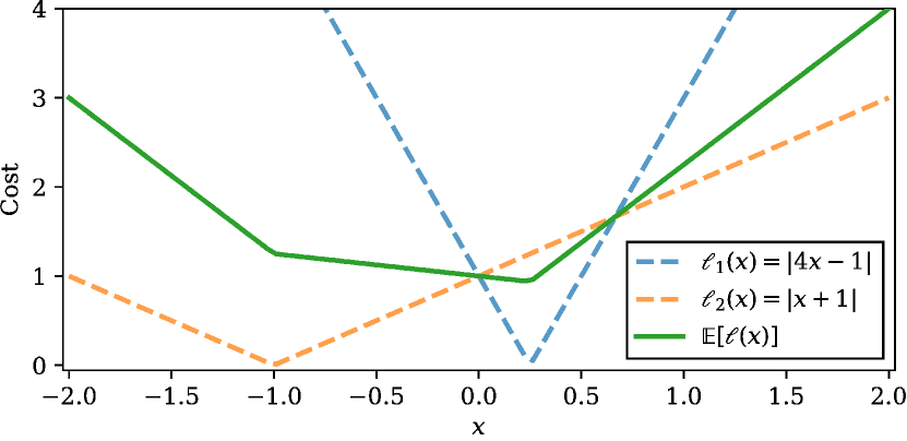
Consider clipping in a stochastic optimization problem. The goal is to optimize where
Hence, and with . The algorithm receives stochastic subgradients
Suppose now that we clip gradients to magnitude . This results in clipped gradients distributed as
which are indistinguishable from the stochastic subgradients of
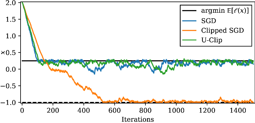
Set . Any algorithm that takes subgradients and is guaranteed to converge on arbitrary stochastic convex optimization problems (e.g. SGD with some learning rate) must converge to if it instead receives the clipped gradients, but and . An empirical example of this aliasing phenomenon is given in Figure 1.
1.2 Related Work
Gradient clipping has had widespread applications for some time [20], is important in training large language models [22, 5] and plays a key role in differentially private optimisation [1]. It is often motivated by control over the update size in the presence of large gradients. Alternatives are normalized gradient descent [12] (closely related to norm clipping) and adaptive step size methods [7, 15]. Adaptive choice of the clip region has been studied for norm clipping [2] and coordinate-wise clipping [21]. Recently, gradient clipping was a component in achieving strong generalisation performance with full batch gradient descent [8].
The convergence of gradient clipping in the deterministic setting with a convex and smooth objective is well known (e.g. one can use [3, Lemma 3.4 ]). Convergence under a relaxation of this smoothness condition is given for norm clipping by [27], who also study the stochastic case, finding faster convergence for clipped SGD than vanilla SGD in their setting. Their work is extended by [26], taking momentum into account. [4] give a convergence proof for norm clipping in SGD for convex smooth functions, quantify the bias due to norm clipping and propose using perturbed gradients to mitigate it. A high probability convergence bound for norm clipped SGD on convex smooth objectives with heavy-tailed gradient noise is given by [10]. [18] prove convergence guarantees for SGD with norm clipping on convex functions arbitrary growth in the subgradients (provided the objective grows faster than a quadratic), but some of their results require the clip region to increase over time, potentially making the clipping redundant.
2 Theory
General Assumptions and Notation.
Our results share some basic assumptions and notation, which we state once here to avoid repetition. We assume is a sequence of convex functions where is convex and is a stochastic subgradient of and with and . This implies that . We assume that each coordinate of is bounded in magnitude by and that the are conditionally independent for given and . We assume that that is sub-Gaussian with variance proxy (of course, sub-Gaussianity is provided by boundedness). It is possible that depends on . Sometimes the clip region will be a scalar, in which case the same clip region is used for each coordinate, other times it will be a vector specifying coordinate-wise clip regions. We will often assume so that we clip noise in the gradients but not the signal, our theory is specifically aimed at this setting and we do not study the regime in which the signal is clipped. The bound on the gradients means we are free to apply the bound for each coordinate, since is a no-op. We will frequently abuse notation by writing for and which is to be interpreted component-wise, i.e. for , and where is a scalar which is to be interpreted component-wise. We will study the average regret, defined by where .
2.1 Convergence Results
In this section we give an overview of our main results, which are regret bounds for U-Clip with various clipping schedules .
Theorem 2.1 is the special case of Theorem 6.1 with the clip region an (absolute) constant. In these results is a scalar representing the same clip region for each coordinate. Per-coordinate clip regions are possible by applying Proposition 2.4 element-wise in the proof of Theorem 6.1.
Theorem 2.1.
Consider U-Clip with learning rate and clipping regions component-wise. The expected average regret is bounded by
where and .
Theorem 2.1 stems from Lemma 2.3 which requires a bound on the carry. If becomes 0, then the carry is a random walk which may diverge in expectation. A factor of appears because the clipping is element-wise, but note that the bound on the norm of the gradients is . It’s possible that this factor would not appear in the corresponding result for norm clipping.
In respect of the more general Theorem 6.1 with time-varying , it may be possible to craft the sequence such that as the gradients . In which case U-Clip would be asymptotically unbiased.222This is not possible in all circumstances, e.g. .
We loosely define adaptive clipping as any clip region schedule that adapts to the noise in the gradients. We now give a convergence result for an instance of adaptive clipping that allows us to improve the dependence on , in particular by taking for .333Unfortunately, this clip region is not scale equivariant, so for our practical experiments we prefer regions of the form (covered by Theorem 6.1, if one has a constant lower bound on ). A direct argument with this (scale equivariant) clip region is likely possibly, albeit by different techniques.
Theorem 2.2 (Adaptive U-Clip).
Consider U-Clip with clip regions (component-wise) for and learning rate . Suppose there is a constant . Then the expected regret is bounded by
Proof.
Identical to the proof of Theorem 6.1 but using WLOG and instead applying Proposition 2.6 to get . ∎
2.2 Gradient Transformations
At the base of our analysis is the following lemma, which may be of independent interest. It says that in the stochastic-online setting with an additive update rule, if the cumulative difference between the updates and the subgradients remains bounded, then the regret of the update rule is also bounded. Intuitively, if an update rule is globally sufficiently similar to gradient descent, then it enjoys the same convergence rate. Note that the gradient descent rate can be achieved with and (defined in the lemma) constant.
Lemma 2.3 (Gradient Transformation).
Let be a sequence of convex functions where . Consider the update equations
where is a stochastic subgradient of at satisfying , and is the learning rate. We call the first sequence the iterates and the second the carry. Set . Suppose that the updates are bounded almost surely by , and let be a non-decreasing sequence.
-
1)
If the carry is bounded in expectation for then the expected (average) regret is bounded by
-
2)
Recall the definition . Suppose that the variables (independent by assumption) are sub-Gaussian with variance proxy . Assume also that the iterates are bounded . Then if with probability at least , then with probability at least we have
The proof is in Section 6.3. Some remarks are in order. First, although sufficient, the condition bounded (either in expectation or in high probability) is not necessary for convergence. For instance there is the trivial situation and with zero regret but . Second, in the case of U-Clip we assume bounded gradients, so we may always take the clipping region , hence the terms in Lemma 2.3 can be treated, albeit crudely, by and . Third, from Lemma 2.3, the condition is sufficient for convergence. Note that this is the same condition required for U-Clip to be unbiased on average (c.f. Section 1). Finally, an alternative version of Lemma 2.3 with a -norm bound on the carry is easily available by using Hölder’s inequality rather than Cauchy-Schwarz towards the end of the proof.
2.3 Carry Bounds
In this section we give bounds on the carry for component-wise clipping for clip regions satisfying element-wise. In particular, the may be chosen as a function of past gradients as long as the sequence is bounded and the above assumption is satisfied. We leave a carry bound for norm clipping to future work. Using Lemma 2.3 we can translate bounds on the carry of update rules into convergence results. For instance, if and then the expected regret is . Note that when doing this, we do not need to apply a union bound over . We have previously assumed that the functions are convex. By inspecting the proofs, the reader will find that this assumption is not necessary for the carry bounds in this section.
The bounds are given for scalar variables, but the results can be applied to control either by a union bound over the co-ordinates (not time) or by application of the expectation results in Propositions 2.4 and 2.6. Doing this introduces an additional factor of the dimension . Results for component specific clip regions can be obtained this way. The idea of the proofs in this section is that it is sufficient to consider the behavior of when it is large and not worry about fine-grained behavior around 0. The proof of Proposition 2.4 is in Section 6.4. A proof sketch is given below. Notice that when the carry becomes a random walk, consistent with the divergence in the bound.
Proposition 2.4 (Carry bound: component-wise clipping).
In this result, all variables are real scalars. Consider the following update rules with
where projects onto the interval . We assume that the sequence satisfies and . Let be a real constant such that . Then for any
where and consequently
Sketch Proof.
If then and clipping is guaranteed on this iteration. This gives . If this happens for iterations then . Using we apply Hoeffding’s inequality, then integrate the bound to get the expectation result. ∎
Corollary 2.5.
Proposition 2.6 below is the carry bound on which Theorem 2.2 relies on. The proof is basically the same but we give it in Section 6.5 for completeness. Although not scale equivariant, it gives a reduced dependence on .
Proposition 2.6 (Carry bound: adaptive clipping).
Set for some . Consider the following update rules with
where projects onto the interval . Suppose there is a constant . Then with probability at least , setting and we get
It follows that
Remark 2.7 (Proportional adaptive clipping).
We define proportional adaptive clipping by the clip region . In Proposition 2.6 this can be achieved by an assumption that the gradient noise variance scales with . However, we can still say something without assumptions on the noise. If is bounded by a constant then we know from Lemma 2.3 that the regret of the average iterate is . On the other hand, if is unbounded in then by comparison with Proposition 2.4 we see that , which in turn implies that the algorithm converges (qualitatively) on a domain of diameter by linearisation
If, in addition, we know that for some sequence , then we get that from the bound on in Proposition 2.4 which gives a rate.
3 Experiments
3.1 Validation of Theoretical Results
In this section we analyze the results from Section 2 empirically on a simple example. We run SGD with U-Clip for 10k iterations, initialized at with learning rate and other parameters varying. The (expected) objective is and the algorithm receives stochastic sub-gradients where is independent, symmetric uniform noise. In this problem, the maximal gradient is related to the noise level (the bounds on the uniform distribution), which in turn is related to the variance (or variance proxy). We use the formula where . This is the basic estimate of the sub-Gaussian variance proxy for any bounded random variable, which is why we use it (despite it not being tight for the uniform distribution).
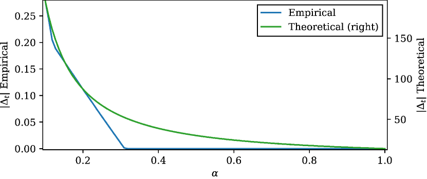
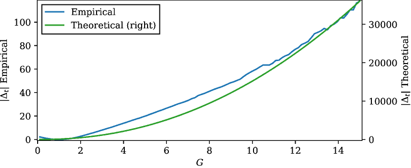
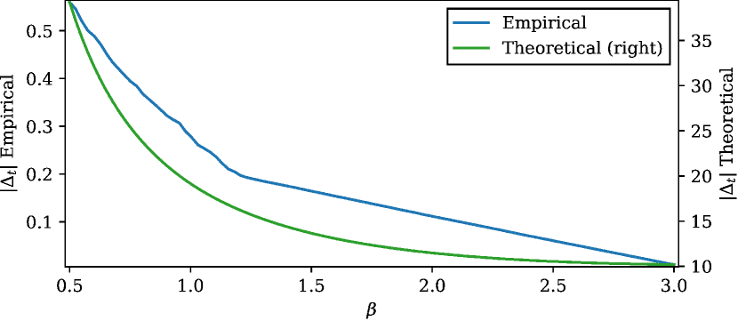
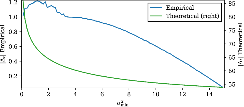
In Figures 2 and 3 we report our validation results for Propositions 2.4 and 2.6 respectively. The charts compare the high probability bounds for at failure rate to the empirical 99th percentile. We vary each parameter independently. In general, up to a constant scaling, we see good agreement between prediction and experiment.
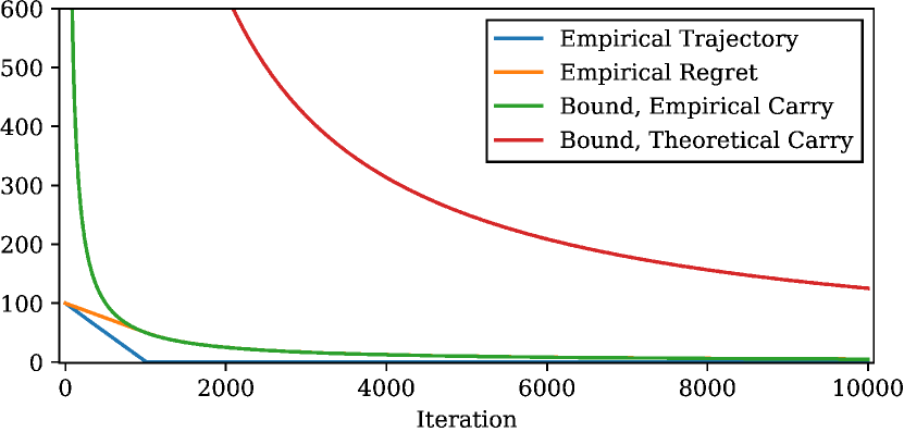
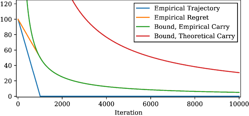
In Figure 4 we validate Lemma 2.3 with expected carry bounds coming from Propositions 2.4 and 2.6 respectively. We report the regret bound from Lemma 2.3 with both the predicted expected carry and the observed carry, finding that the regret bound is essentially tight in the latter case (so the slack in the overall result comes from the expectation bound). In a way this is to be expected, because saturates the linearised analysis in Lemma 2.3.
3.2 Practical Performance
In this section we report the performance of U-Clip when combined (as described in Section 1) with standard optimizers (SGD, momentum, Adam) to optimize a small conv-net on CIFAR10 [17]. We also provide validation for using U-Clip with momentum to train a ResNet50v2 on ImageNet [6]. We compare the performance of U-Clip to that of the base optimizer and of the base optimizer with clipping (but no carry). The purpose of this section is to demonstrate that U-Clip works in practical settings. Although U-Clip does outperform the base optimizer in some settings, we make no attempt to achieve state of the art results.
We explore the performance of various clipping regimes: component clipping and norm clipping with constant (same region for each parameter), and component clipping with clip region chosen adaptively as a function of past gradients. In the adaptive case, we use for where and are component-wise estimates of the mean and standard-deviation of each parameter respectively.
We consider two methods of estimation. The first is the sample variance using Welford estimation with the standard iterative calculation of the sample mean, then using . The second is exponentially weighted moving average (EWMA) of the first and second moments with decay factor , then using .
3.2.1 CIFAR10
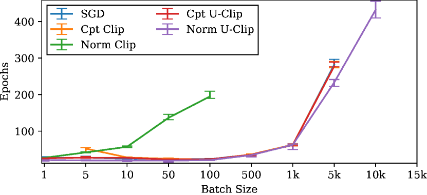
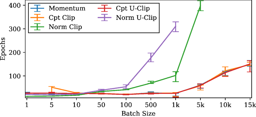
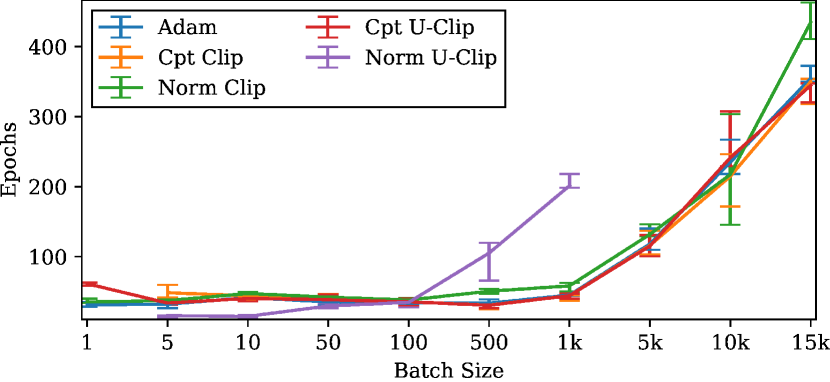
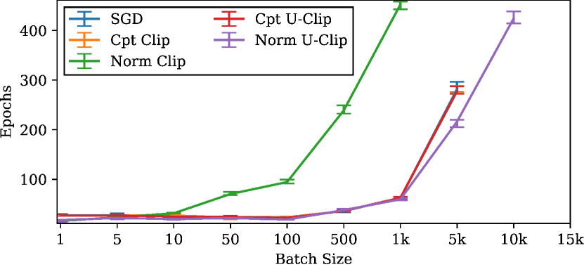
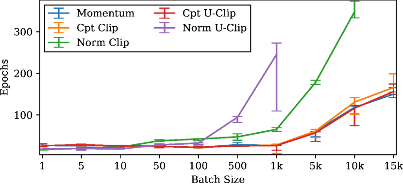
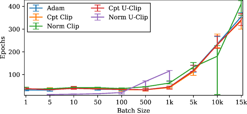
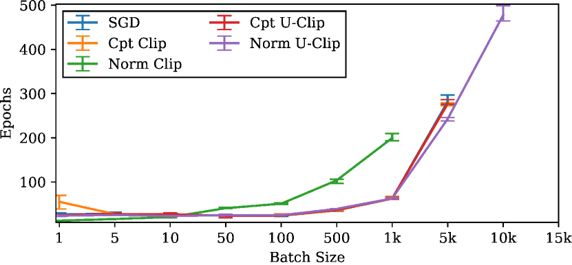
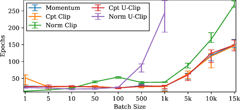
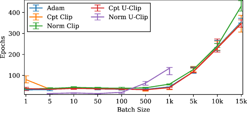
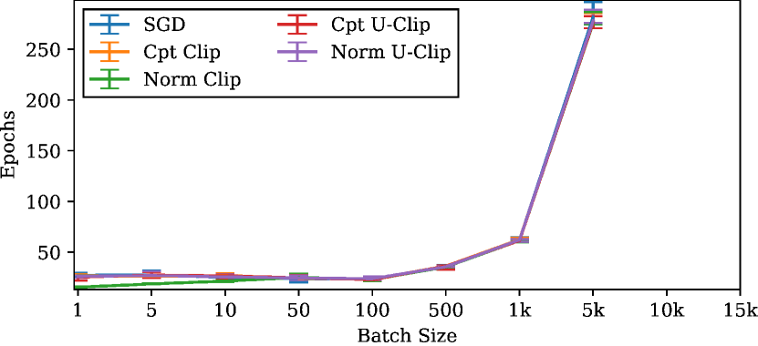
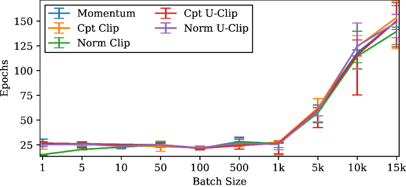
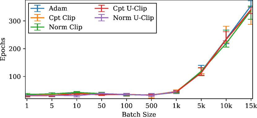
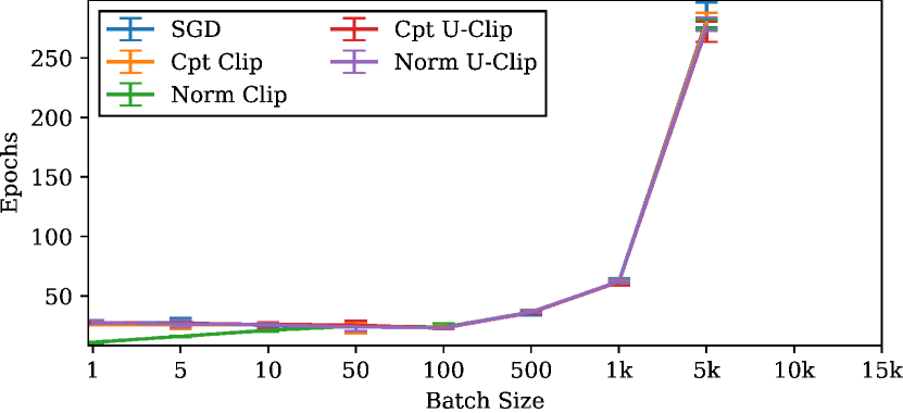
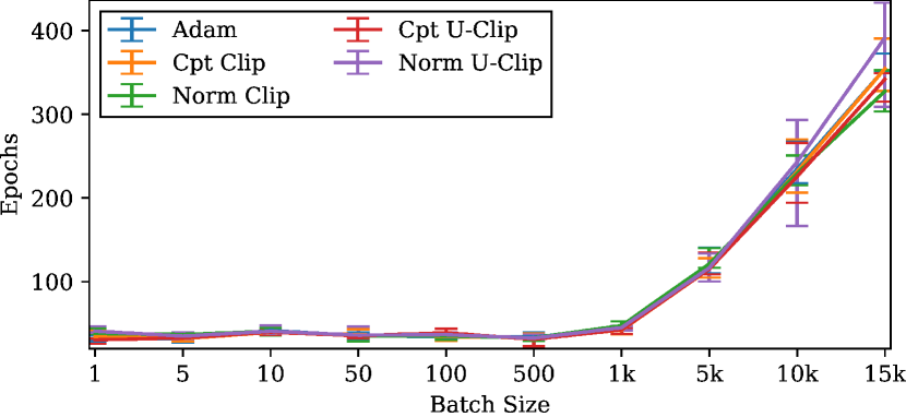
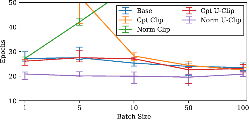
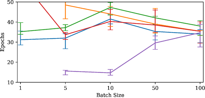
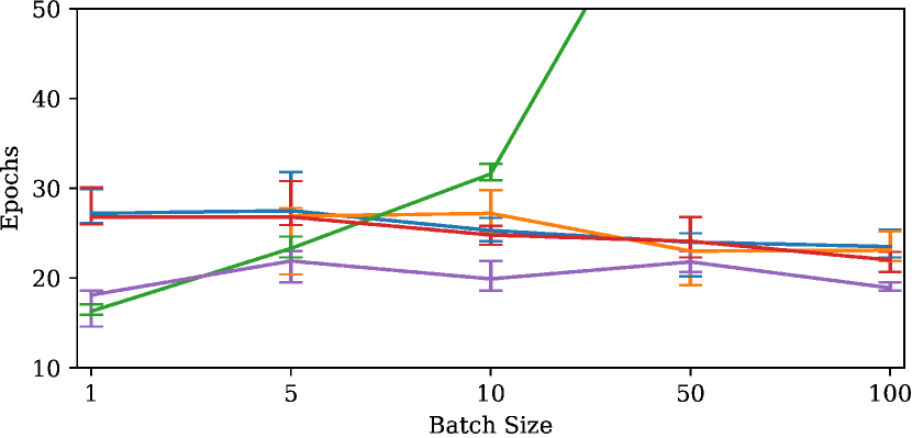
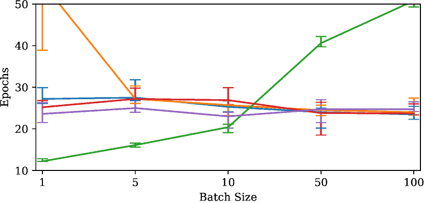
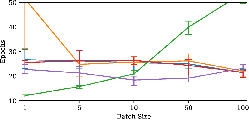
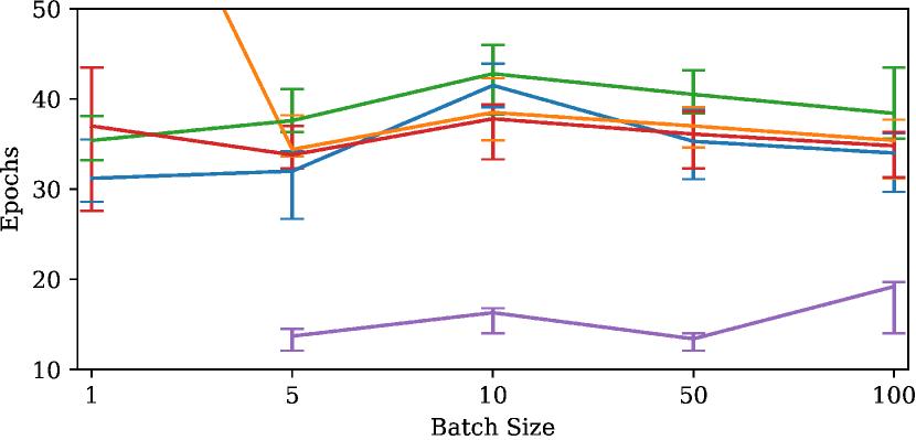
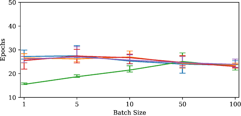
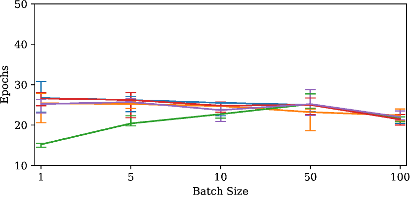
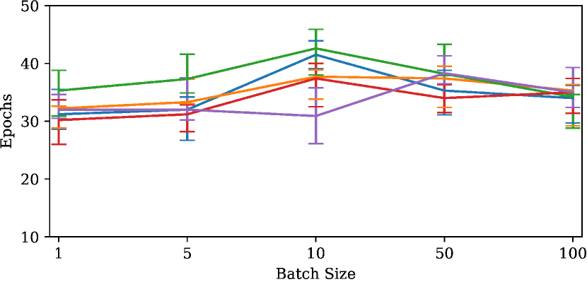
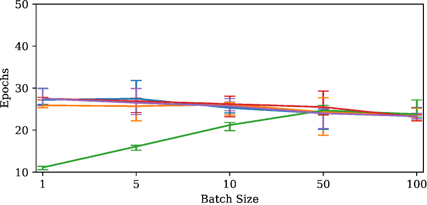
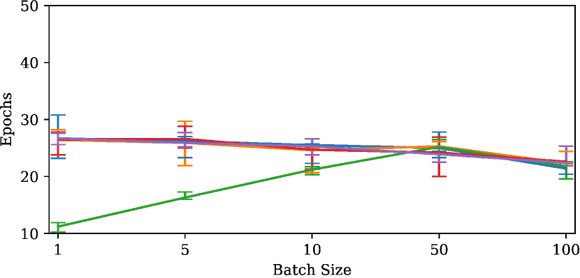
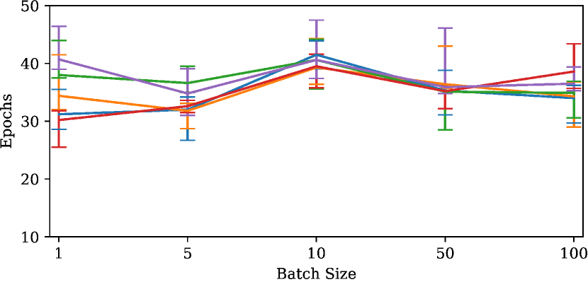
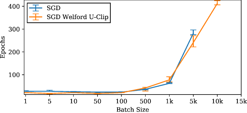
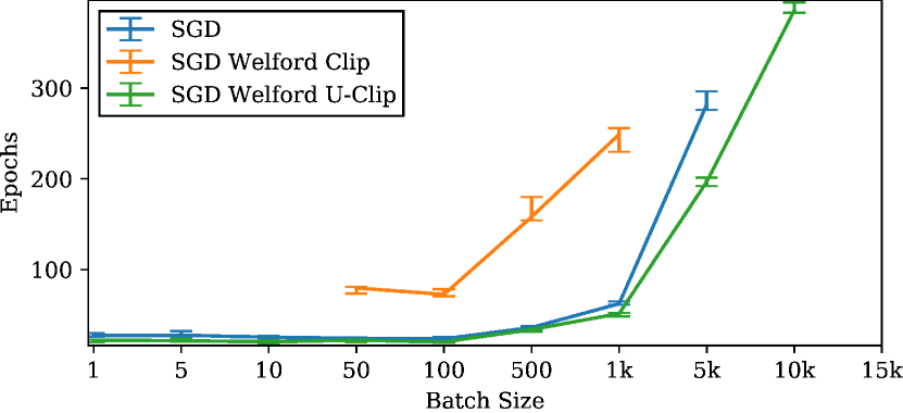
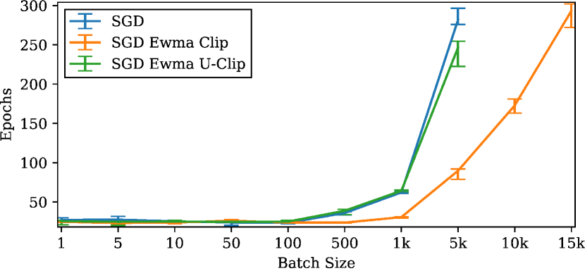
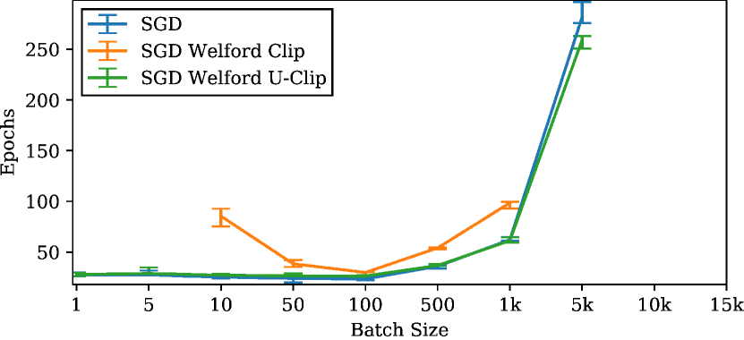
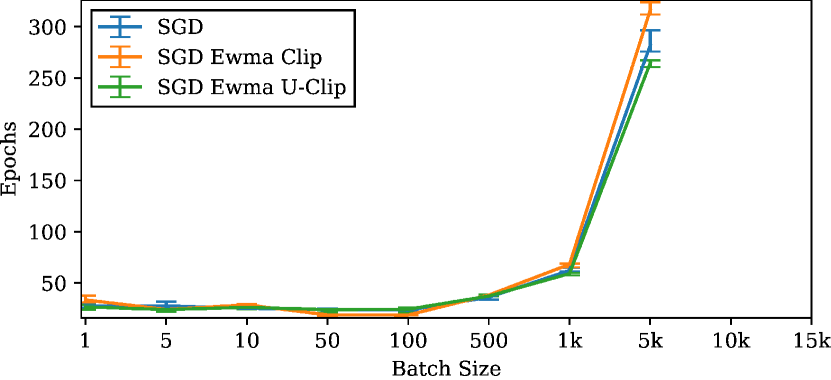
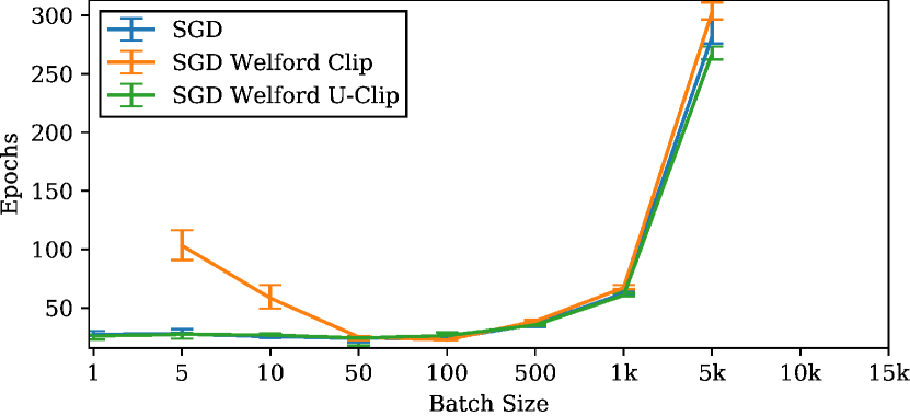
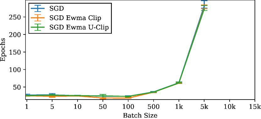
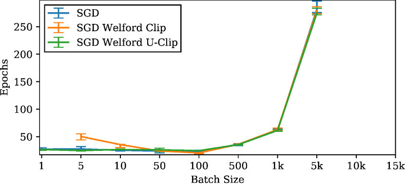
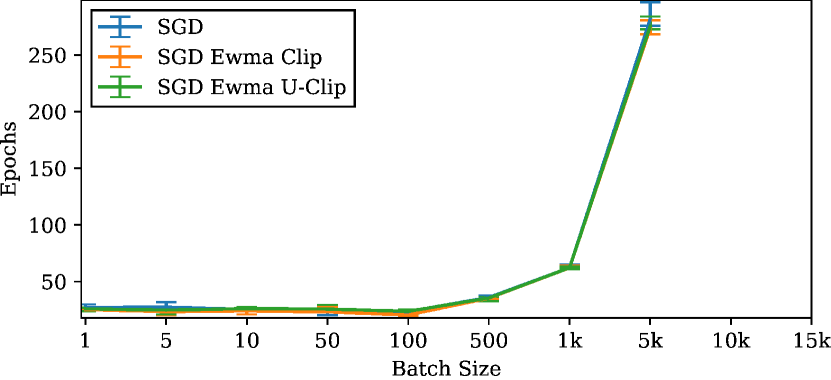
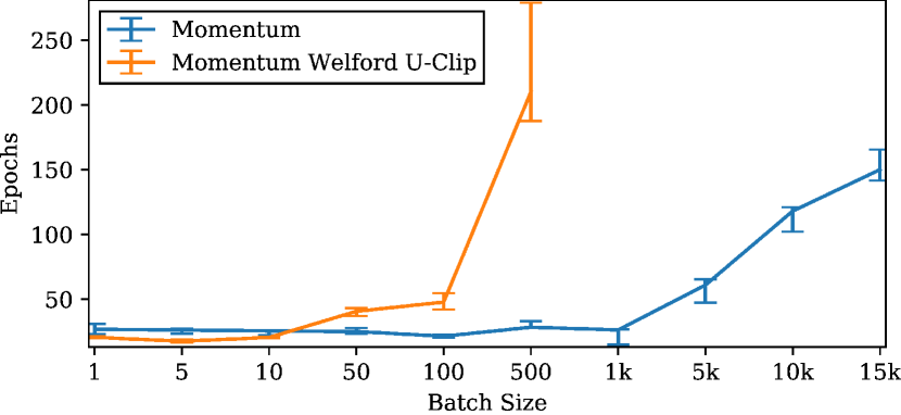
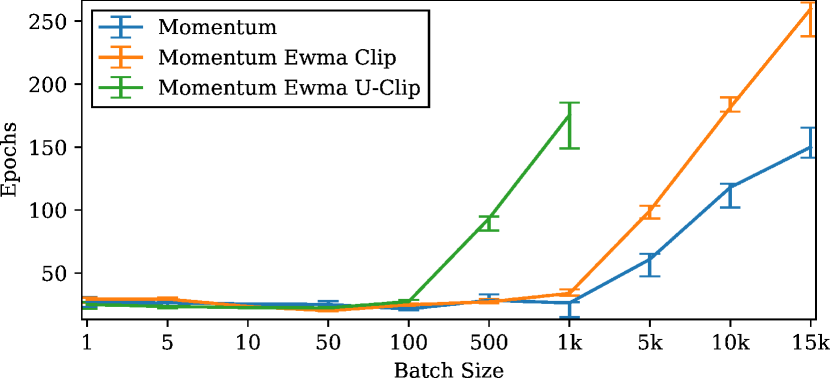
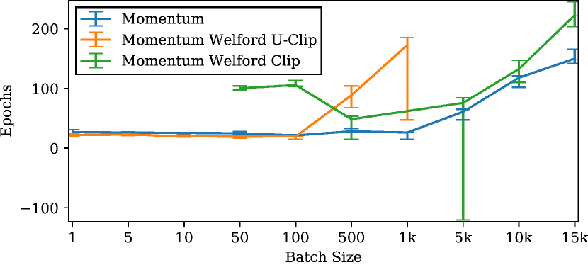
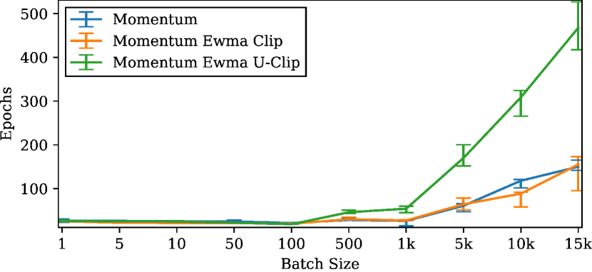
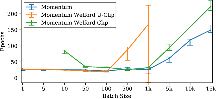
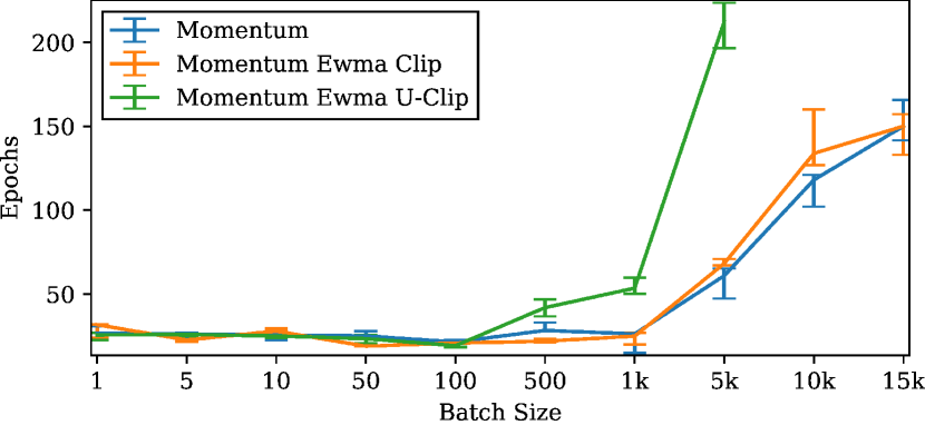
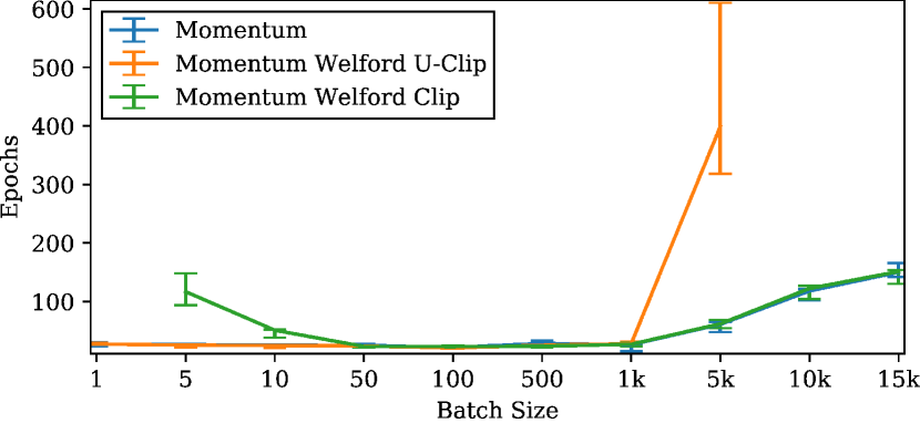
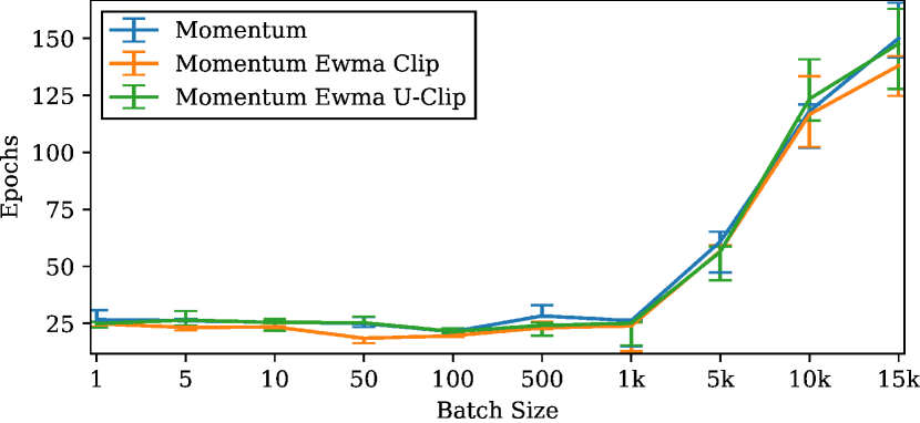
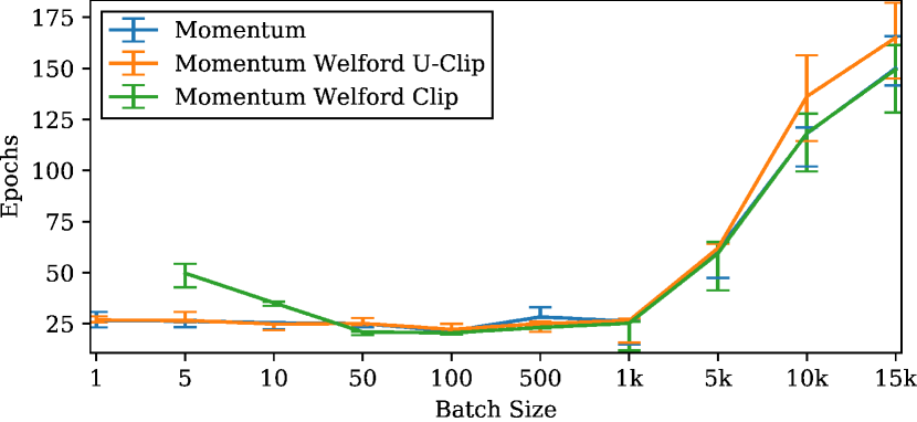
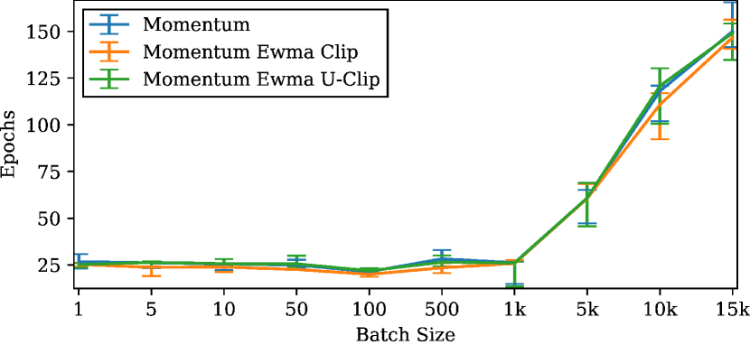
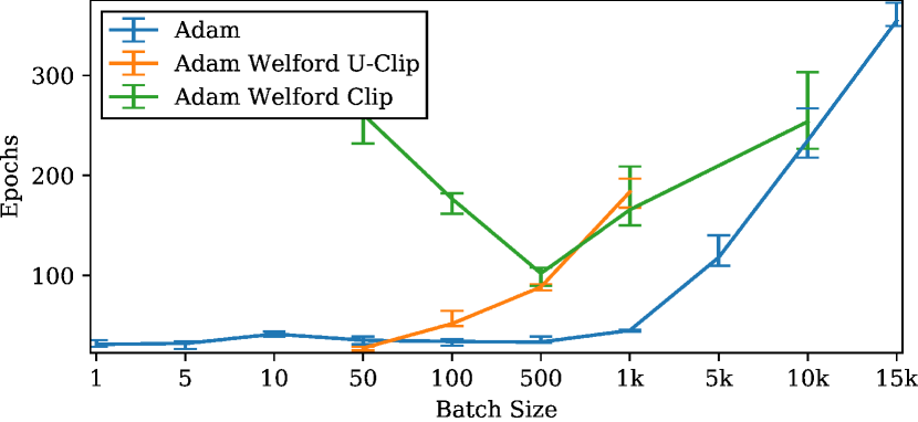
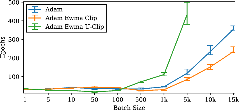
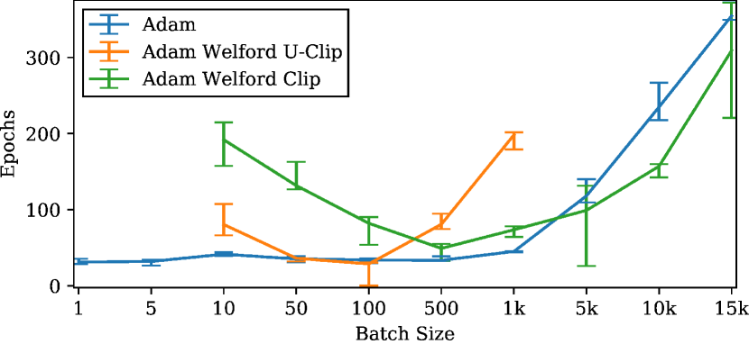
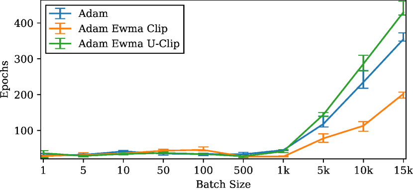
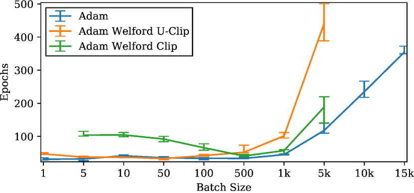
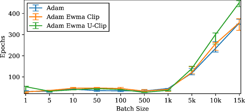
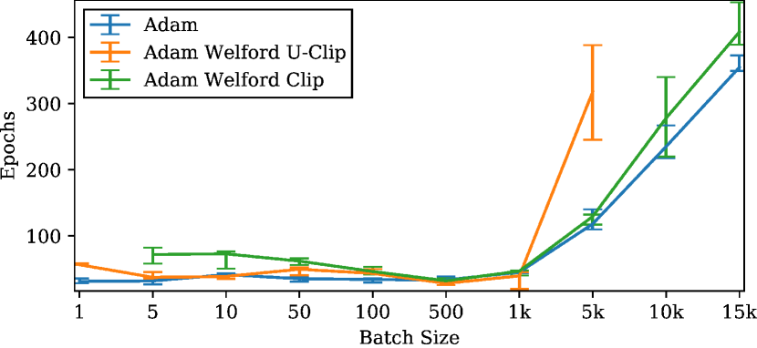
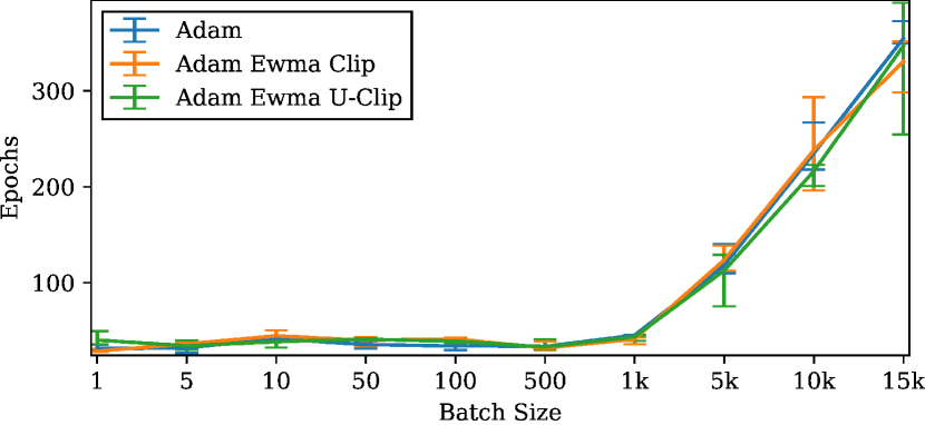
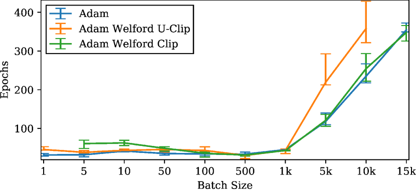
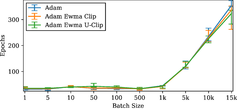
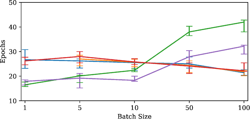
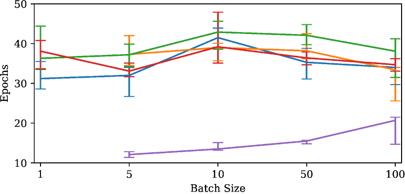
We train a small convolutional net on the CIFAR10 dataset to minimize the cross-entropy loss. We explore the performance of U-Clip in combination with SGD, momentum (parameter ) and Adam (parameters and ). We refer to these as the base optimizers. We calculate the median, minimum and max number of epochs needed to reach 99% training accuracy for each configuration over 5 seeds. The learning rate is tuned to the batch size according to the median (smaller is better) across 5 log-spaced values. Further experimental details are given in Section 7.1
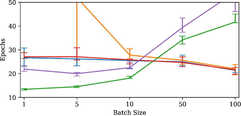
We report a selection of the results here with the rest in Section 9. We find that for smaller batch sizes ( 100) U-Clip rarely slows optimization when compared to the base optimizer and sometimes gives a significant advantage. On the other hand, for large batch sizes the carry seems to slow training or make it less stable. We believe the benefit for small batch sizes, as shown in Figure 5, is due to the memory of the carry smoothing out mini-batch noise. For small batch sizes this noise is prevalent so the carry is helpful. With larger batch sizes large gradients are more likely due (possibly transitory) large signals from the underlying expected objective. In this case the carry is harmful because a region of large gradients could make the carry large for many iterations.



3.2.2 ImageNet
We validate the performance of U-Clip on a larger scale experiment, training a ResNet50v2 [13] on ImageNet with Nesterov momentum. We modify a base setup by adding clipping and U-Clip for the following clip regions: constant , adaptive and proportional adaptive clipping . In each adaptive case we use each of Welford (sample mean/variance) and EWMA estimation (decay 0.95) as in Section 3.2.1. Further experimental details are given in Section 7.2
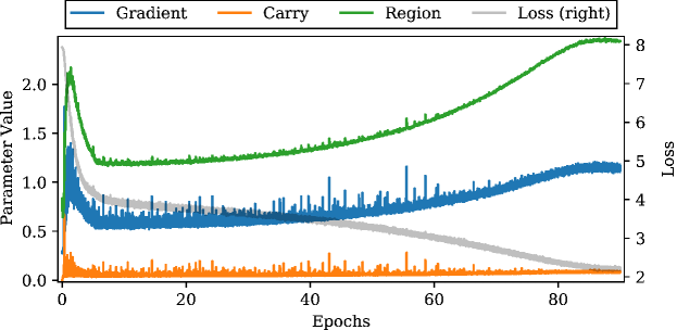
We run each configuration for 5 seeds and report the median and min/max range over the seeds of the best top 1 accuracy on a validation set. The results are presented in Table 1 and a sample optimization trajectory is given in Figure 6. We find it encouraging that U-Clip proves to be competitive with the base setup, but it does not provide significant benefit under these conditions, possibly because the batch size is relatively large. We made no attempt to tune the base setup according to the modifications, so it is likely that improvements on the results shown are possible. Time and resource constraints mean we must leave further exploration to future work.
| Median | Range | Clip Region | Carry | or |
|---|---|---|---|---|
| 77.2% | Welford | True | ( 1 , 2) | |
| 77.2% | EWMA | True | ( 1 , 2 ) | |
| 77.2% | Component | True | 0.25 | |
| 77.1% | Component | False | 0.25 | |
| 77.1% | EWMA | False | ( 1 , 2 ) | |
| 77.1% | No Clipping | - | - | |
| 77.0% | EWMA | False | ||
| 76.9% | Welford | False | ||
| 76.8% | EWMA | True | ||
| 76.2% | Norm | False | 0.25 | |
| 75.6% | Norm | True | 0.25 | |
| 72.7% | Welford | False | ||
| 61.2% | Welford | True |
4 Conclusion
We have presented U-Clip, a novel method for achieving on-average unbiased stochastic gradient clipping. U-Clip has desirable theoretical properties and solid empirical validation. The simplicity of U-Clip allows for solid theoretical analysis using elementary techniques, which we see as a key strength. In addition, our initial investigations find empirical performance that is competitive with standard methods, warranting further study. We hope that the reader is motivated to experiment with and extend U-Clip. We give suggestions for future work in Section 5.
Acknowledgements
This work was performed while BE was an intern at DeepMind. We would like to thank, in alphabetical order, the following people for helpful conversations and support: András György, Charline Le Lan, Claire Vernade, Denizalp Goktas, Flore Sentenac, Ilja Kuzborskij, Laurent Orseau, Mihaela Rosca, Sahra Ghalebikesabi and Sam Smith, and especially Ilja for valuable feedback on drafts.
References
- [1] Martin Abadi et al. “Deep learning with differential privacy” In Proceedings of the 2016 ACM SIGSAC conference on computer and communications security, 2016, pp. 308–318
- [2] Galen Andrew, Om Thakkar, Brendan McMahan and Swaroop Ramaswamy “Differentially private learning with adaptive clipping” In Advances in Neural Information Processing Systems 34, 2021, pp. 17455–17466
- [3] Sébastien Bubeck “Convex optimization: Algorithms and complexity” In Foundations and Trends® in Machine Learning 8.3-4 Now Publishers, Inc., 2015, pp. 231–357
- [4] Xiangyi Chen, Steven Z Wu and Mingyi Hong “Understanding gradient clipping in private SGD: A geometric perspective” In Advances in Neural Information Processing Systems 33, 2020, pp. 13773–13782
- [5] Aakanksha Chowdhery et al. “Palm: Scaling language modeling with pathways” In arXiv preprint arXiv:2204.02311, 2022
- [6] Jia Deng et al. “Imagenet: A large-scale hierarchical image database” In 2009 IEEE conference on computer vision and pattern recognition, 2009, pp. 248–255 Ieee
- [7] John Duchi, Elad Hazan and Yoram Singer “Adaptive subgradient methods for online learning and stochastic optimization.” In Journal of machine learning research 12.7, 2011
- [8] Jonas Geiping et al. “Stochastic training is not necessary for generalization” In arXiv preprint arXiv:2109.14119, 2021
- [9] Xavier Glorot and Yoshua Bengio “Understanding the difficulty of training deep feedforward neural networks” In Proceedings of the thirteenth international conference on artificial intelligence and statistics, 2010, pp. 249–256 JMLR WorkshopConference Proceedings
- [10] Eduard Gorbunov, Marina Danilova and Alexander Gasnikov “Stochastic optimization with heavy-tailed noise via accelerated gradient clipping” In Advances in Neural Information Processing Systems 33, 2020, pp. 15042–15053
- [11] Moritz Hardt, Ben Recht and Yoram Singer “Train faster, generalize better: Stability of stochastic gradient descent” In International conference on machine learning, 2016, pp. 1225–1234 PMLR
- [12] Elad Hazan, Kfir Levy and Shai Shalev-Shwartz “Beyond convexity: Stochastic quasi-convex optimization” In Advances in neural information processing systems 28, 2015
- [13] Kaiming He, Xiangyu Zhang, Shaoqing Ren and Jian Sun “Identity mappings in deep residual networks” In European conference on computer vision, 2016, pp. 630–645 Springer
- [14] Pooria Joulani, Andras Gyorgy and Csaba Szepesvári “Delay-tolerant online convex optimization: Unified analysis and adaptive-gradient algorithms” In Proceedings of the AAAI Conference on Artificial Intelligence 30.1, 2016
- [15] Diederik P Kingma and Jimmy Ba “Adam: A method for stochastic optimization” In arXiv preprint arXiv:1412.6980, 2014
- [16] Günter Klambauer, Thomas Unterthiner, Andreas Mayr and Sepp Hochreiter “Self-normalizing neural networks” In Advances in neural information processing systems 30, 2017
- [17] Alex Krizhevsky and Geoffrey Hinton “Learning multiple layers of features from tiny images” Toronto, ON, Canada, 2009
- [18] Vien V Mai and Mikael Johansson “Stability and convergence of stochastic gradient clipping: Beyond lipschitz continuity and smoothness” In International Conference on Machine Learning, 2021, pp. 7325–7335 PMLR
- [19] Laurent Orseau and Marcus Hutter “Isotuning With Applications To Scale-Free Online Learning” In arXiv preprint arXiv:2112.14586, 2021
- [20] Razvan Pascanu, Tomas Mikolov and Yoshua Bengio “On the difficulty of training recurrent neural networks” In International conference on machine learning, 2013, pp. 1310–1318 PMLR
- [21] Venkatadheeraj Pichapati et al. “AdaCliP: Adaptive clipping for private SGD” In arXiv preprint arXiv:1908.07643, 2019
- [22] Jack W Rae et al. “Scaling language models: Methods, analysis & insights from training gopher” In arXiv preprint arXiv:2112.11446, 2021
- [23] Herbert Robbins and Sutton Monro “A stochastic approximation method” In The annals of mathematical statistics JSTOR, 1951, pp. 400–407
- [24] Umut Simsekli, Levent Sagun and Mert Gurbuzbalaban “A tail-index analysis of stochastic gradient noise in deep neural networks” In International Conference on Machine Learning, 2019, pp. 5827–5837 PMLR
- [25] Ilya Sutskever, James Martens, George Dahl and Geoffrey Hinton “On the importance of initialization and momentum in deep learning” In International conference on machine learning, 2013, pp. 1139–1147 PMLR
- [26] Bohang Zhang, Jikai Jin, Cong Fang and Liwei Wang “Improved analysis of clipping algorithms for non-convex optimization” In Advances in Neural Information Processing Systems 33, 2020, pp. 15511–15521
- [27] Jingzhao Zhang, Tianxing He, Suvrit Sra and Ali Jadbabaie “Why gradient clipping accelerates training: A theoretical justification for adaptivity” In arXiv preprint arXiv:1905.11881, 2019
- [28] Xinwei Zhang, Xiangyi Chen, Mingyi Hong and Zhiwei Steven Wu “Understanding clipping for federated learning: Convergence and client-level differential privacy” In arXiv preprint arXiv:2106.13673 2, 2021
5 Suggestions for Future Work
-
•
Extension of theory to unbounded gradients, possibly with heavy-tailed noise which could be particularly relevant in deep learning [24].
- •
-
•
Extension of Lemma 2.3 to time varying learning rate and tuning the learning rate to get a scale free bound, possibly using techniques from [19]. In addition, one could adapt Lemma 2.3 to achieve convergence to a stationary point on non-convex functions. Our results could also be generalized to the minibatch setting.
-
•
Generalize carry bounds to online (not necessarily stochastic) setting. One could use the historical sample mean/variance of gradients as analogues for the statistical quantities and , e.g. .
-
•
Investigate relationship of U-Clip to Follow the Regularized Leader with delayed feedback [14].
-
•
Tuning of the experiments to give optimal performance and experiments on large language models, where clipping is particularly relevant.
-
•
U-Clip in alternative application domains, such as reward clipping in reinforcement learning.
-
•
Exploration, both theoretical and empirical, of alternative clipping schemes. For instance symmetric clipping, where the gradient is clipped to some interval (e.g. standard deviations) centred on an estimate of .
-
•
Exploration of U-Sign, in which the function is replaced element-wise. This gives the update equations (c.f. Equation 1 and surrounding description)
While clipping helps with the exploding gradient problem, U-Sign would also help prevent vanishing updates. Like U-Clip, it may be on-average unbiased.
6 Additional Theoretical Results
6.1 Convergence Result
Recall that WLOG we are free to take element-wise.
In Theorem 6.1, is a scalar specifying the same clip region for each coordinate. Per-coordinate clip regions are possible by applying Proposition 2.4 element-wise in the proof.
Theorem 6.1 (U-Clip convergence: component-wise clipping).
Consider U-Clip with learning rate and clipping regions component-wise. The expected regret is bounded by
where , , and .
Proof of Theorem 6.1.
We may apply Proposition 2.4 element-wise to . For any
by a union bound and the bound on in the statement of Proposition 2.4. The same calculation from the proof of Proposition 2.4 then gives
We can now apply Lemma 2.3 with to bound the the expected regret of U-Clip. Observe that and . We define and . With this, item 1 of Lemma 2.3 becomes
which, upon substituting in and using the definition of , becomes
∎
6.2 Omitted Proofs
We restate the results for the reader’s convenience.
6.3 Proof of Lemma 2.3
Lemma (Lemma 2.3).
Let be a sequence of convex functions where . Consider the update equations
where is a stochastic subgradient of at satisfying , and is the learning rate. We call the first sequence the iterates and the second the carry. Set . Suppose that the updates are bounded almost surely by , and let be a non-decreasing sequence.
-
1)
If the carry is bounded in expectation for then the expected (average) regret is bounded by
-
2)
Recall the definition . Suppose that the variables (independent by assumption) are sub-Gaussian with variance proxy . Assume also that the iterates are bounded . Then if with probability at least , then with probability at least we have
Proof of Lemma 2.3.
We start by using the subgradient inequality following from the convexity of the and then use the parallelogram rule for inner products
Then, also by convexity and using the assumption on the updates,
| () |
almost surely. Using and the update rule we consider the first term,
almost surely. Putting this back into Equation gives
| () |
We complete the proof by specializing Equation to the two cases in the statement.
First 1. The final term in Equation has mean 0, since by the law of total expectation . So taking expectations and using the condition along with gives the result.
Now item 2. With probability at least , . Along with non-decreasing this gives, from Equation
It remains only to control the final term. We have and that the quantity is sub-Gaussian with variance proxy : for any
The standard tail bound (Hoeffding) then gives
The result is immediate from a simple calculation and a union bound. ∎
6.4 Proof of Proposition 2.4
Proposition (Proposition 2.4).
In this result, all variables are real scalars. Consider the following update rules with
where projects onto the interval . We assume that the sequence satisfies and . Let be a real constant such that . Then for any
where and consequently
Proof of Proposition 2.4.
For any time and for , we define the events
with . Note that . The update rule is
If happens then . There is now only one possibility for . In particular, if then , and similarly if then so , hence we must instead have . Using this and the same idea iteratively, then using the expression for the gradients, it follows that implies
So
By conditioning on the history we may exploit independence and use Hoeffding’s inequality with to get
Then
| () | ||||
Using the same method, one can calculate that
and the result follows from a union bound.
To calculate the expectation, we will use the weaker form
Then
∎
6.5 Proof of Proposition 2.6
Proposition (Proposition 2.6).
Set for some . Consider the following update rules with
where projects onto the interval . Suppose there is a constant . Then with probability at least , setting and we get
It follows that
Proof of Proposition 2.6.
Define . For any time and for , we define the events
with . Note that . The update rule is
If happens then . There is now only one possibility for . In particular, if then , and similarly if then so , hence we must instead have . Using this and the same idea iteratively, then using the expression for the gradients, it follows that implies
So
Assume temporarily that , then by assumption on and Hoeffding’s inequality we have
Where . Now note that if then almost surely and the above result remains true. Using for any event and -field we integrate out and get
Using the same method one can calculate that . Then and a union bound gives
from which the first result is immediate. Doing the same integration at end of the proof of Proposition 2.4 and using gives
∎
7 Additional Experimental Details
7.1 CIFAR10
The network has two convolutional layers with 32 and 64 features respectively, initialized with the LeCun normal initialization, also known as the truncated normal initialization [16], with initial bias 0. Each convolutional later has a kernel and followed by average pooling over a window with strides. The convolution layers are follows my fully connected layers with features of width , initialized with Gaussian Glorot initialization [9] and initial bias of . All of the activations are ReLU.
Each experiment is run for 5 random seeds on a V100 GPU, with learning rates , , ,, and on on batch sizes 1, 5, 10, 50, 100, 500, 1000, 5000, 10000, 15000 for epochs 100, 300, 300, 300, 300, 500, 500, 500, 500, 500 per batch size (to give enough steps to converge). An experiment consists of training the model using one of the base optimizers either alone, with clipping (no carry) or with U-Clip. In the two cases where clipping is used, we consider component and norm clipping with constant clip region (over time and parameters) , and adaptive clipping with parameters with each of Welford and EWMA estimation.
7.2 ImageNet
The base setup is the Haiku implementation of ResNet50v2 with batch norm (decay rate 0.9) on ImageNet. The network is trained to minimize cross-entropy loss with weight decay () and label smoothing () with Nesterov momentum (decay 0.9) for 90 epochs and a cosine schedule learning rate with initial learning rate 0.1 and 5 warm-up epochs. We train on on a 4x4 TPU pod. Batch size is 128 per device, so 4096 in total.
8 Parallelization
In reference to single program, multiple data parallelization of U-Clip there are two options.444 In the single program, multiple data paradigm, the model is copied across multiple devices, gradients are computed on each device using different training data and the gradients are aggregated on a separate device. This allows for a batch size , sidestepping memory constraints on a single device. One could clip the gradients on each device individually then aggregate, or aggregate the gradients then clip the result.
The benefit of the former is that effect of any spurious/outsized gradients on any device on the aggregate is limited. For instance, maybe only one example on one device is causing issues. In this case, only the examples on the offending device would be affected. One could perform multiple rounds of gradient computations in this way before updating the weights, increasing the overall batch size further.
On the other hand, the latter has the benefit that noise/large values can cancel out “naturally”, maybe obviating the need to clip at all on that iteration. One might also prefer this approach since it interferes with the gradient statistics at the latest possible moment.
9 Additional Experimental Results: CIFAR10
