Maximum likelihood estimator
for skew Brownian motion:
the convergence rate

Antoine Lejay111Université de Lorraine, CNRS, IECL, Inria, F-54000 Nancy, France; ORCID: 0000-0003-0406-9550; Antoine.Lejay@univ-lorraine.fr    Sara Mazzonetto222Université de Lorraine, CNRS, IECL, Inria, F-54000 Nancy, France; ORCID: 0000-0001-6187-2716; Sara.Mazzonetto@univ-lorraine.fr
(March 1, 2024)
Abstract

We give a thorough description of the asymptotic property of the maximum likelihood estimator (MLE) of the skewness parameter of a Skew Brownian Motion (SBM). Thanks to recent results on the Central Limit Theorem of the rate of convergence of estimators for the SBM, we prove a conjecture left open that the MLE has asymptotically a mixed normal distribution involving the local time with a rate of convergence of order $1/4$. We also give a series expansion of the MLE and study the asymptotic behavior of the score and its derivatives, as well as their variation with the skewness parameter. In particular, we exhibit a specific behavior when the SBM is actually a Brownian motion, and quantify the explosion of the coefficients of the expansion when the skewness parameter is close to $-1$ or $1$.

MSC(2020) Classification: Primary 62F12; Secondary 62F03.

Keywords: Skew Brownian motion; maximum likelihood estimator (MLE); statistical estimation; null recurrent process.

Skew and other singular diffusions attract more and more interest in modeling diffusive stochastic behavior in presence of semi-permeable barriers, discontinuities, and thresholds. Beyond theoretical studies, simulation and inference are also necessary tools for practical purposes. For some example of applications in various fields, see e.g. [28, 9, 31, 36, 30, 8, 10, 7, 13] among others.

The inference of skew diffusion cannot follow from a simple adaptation of known techniques for Stochastic Differential Equations (SDE) as the ones presented in [12, 15]. In fact their distributions are singular with the ones of classical SDE. The limits are usually mixed normal ones and the rate is not necessarily $1/2$. The work dealing with the inference of skew diffusion is rather limited. Let us cite however [6, 21, 22, 27, 17, 26, 25, 24, 33, 34] for frequentist inference and [5, 3, 4] for Bayesian inference.

The Skew Brownian motion (SBM) is a basic brick for constructing Skew diffusion, as several transformations reduces Skew diffusions to SBM [16]. This latter process depends on a single parameter $\theta\in[-1,1]$ — the skewness parameter — which rules out its behavior when it crosses zero. For $\theta=0$, the SBM is a Brownian motion. For $\theta=\pm 1$, it is a Reflected Brownian motion.

A series of works considers the inference of the skewness parameter from high-frequency observations. In [21], the authors have given an asymptotic expansion of the Maximum Likelihood Estimator (MLE) $\theta_{n}$ of $\theta$ around $\theta=0$ in power of $n^{-1/4}$, where $n$ is the number of observations. A heuristic explanation of the power $1/4$ is given by analogy with the Skew Random Walk [18], where the MLE depends on the local time at zero of the discrete walk, which a random quantity of order $\sqrt{n}$. Indeed in [22], where the consistency of the MLE and another estimator is proved, it was empirically observed that the rate of convergence should be $1/4$, meaning that the observed points that “carry the information” are those close to 00, and are of order $\sqrt{n}$. This also explains why the asymptotic limit of the MLE involves the local time at 00. The limit is of type $\mathcal{s}(\theta)G/\sqrt{L_{1}}$ (when the process is observed on $[0,1]$), where $(L_{t})_{t\geq 0}$ is the symmetric local time at 00 of the SBM and $G$ is a centered unit, Gaussian independent from the SBM. The value of $\mathcal{s}(\theta)$ was empirically observed as closed to $\kappa\sqrt{1-\theta^{2}}$. It was conjectured in [22] that $\mathcal{s}(\theta)=\kappa\sqrt{1-\theta^{2}}$ as for the Skew Random Walk.

The article [27] brought the missing result required to establish a Central Limit Theorem on the MLE and other estimators. A related result may also be found in [32]. As for the results in [22], this is based on an extension of the work of J. Jacod [14] that cannot be applied directly as the SBM has a singular distribution with respect to the one of the BM.

In this article, we first prove the asymptotic normality of the MLE of the skewness parameter $\theta$ of the SBM. More precisely, we establish that

$$n^{1/4}(\theta_{n}-\theta)\xrightarrow[n\to\infty]{\text{stably}}{}\mathcal{s}(\theta)W(L_{T})\stackrel{{\scriptstyle\mathrm{law}}}{{=}}\mathcal{s}(\theta)\frac{W(1)}{\sqrt{L_{T}}}$$

for a Brownian motion $W$ independent from the SBM. In particular, we show that $\mathcal{s}(\theta)=\kappa(\theta)\sqrt{1-\theta^{2}}$ with a pre-factor $\kappa(\theta)$ that varies slowly.

Second, using a recent asymptotic inversion formula [20], we establish a series expansion of $\theta_{n}$ as

$$\theta_{n}=\theta+\sum_{k=1}^{+\infty}\mathsf{D}_{k,n}(\theta)\left(\frac{\mathcal{s}(\theta)\mathsf{P}_{n}(\theta)}{T^{1/4}n^{1/4}}\right)^{k},$$ (1)

for some random quantities $\mathsf{D}_{k,n}(\theta)$ whose asymptotic behavior is also studied, and $\mathsf{P}_{n}(\theta)$ is asymptotically pivotal (i.e., the asymptotic law does not depend on the parameter). All these results are based on the asymptotic behavior of the score and their derivatives at any orders. Expansion (1) provides some insight on the behavior of the MLE in function of the number of samples $n$ and the true value of $\theta$. In particular, the closer $\theta$ is to $\pm 1$, the more skewness is observed.

Furthermore, we show that $\mathsf{D}_{2k+1,n}(\theta=0)$ converges to 00 so that a more precise expression of the involving a multivariate mixed Gaussian distribution could be given for the MLE of $\theta=0$. This expression is an alternative to the one already given in [21].

Moreover, we give some numerical experiments on the rate of convergence of the distribution functions of the MLE and the score and its derivatives towards their limiting distributions. The rate of convergence of this Berry-Esseen type analysis seems to depend on $\theta$. This will be subject to further study.

Finally, we study the behavior of the limiting coefficients in function of $\theta$. In particular, the expansion in (1) exhibits a boundary layer estimate for $\theta$ close to $\pm 1$ as the coefficients explode in powers of $(1-\theta^{2})^{-1/2}$.


Outline. We present our main results in Section 1. They are built on the asymptotic behavior of the score and its derivative which we give in Section 2. We also study numerically the rate of convergence of the scores and their derivatives towards their limits in Section 2.1. The properties of the limiting coefficients are studied in Section 3. And the proofs of our main theorems are given in Section 4.

1 Main results

The SBM $X$ of parameter $\theta\in[-1,1]$ solves the SDE

$$X_{t}=B_{t}+\theta L_{t},\ t\geq 0$$ (2)

for $B$ a Brownian motion and $\{L_{t}\}_{t\geq 0}$ its symmetric local time of $X$ at point 00. Actually, the SDE (2) has a unique strong solution [16, 11]. No solution exists when $|\theta|>1$. For $\theta=\pm 1$, the SBM is a (positively if $\theta=1$ or negatively if $\theta=-1$) Reflected Brownian motion.

We denote by $(\Omega,\mathcal{F},\mathbb{P}_{\theta})$ the underlying probability space and by $\{\mathcal{F}_{t}\}_{t\geq 0}$ the filtration with respect to which $X$ is adapted. This filtration may be taken as the one generated by the driving Brownian motion and may be assumed to satisfy the usual conditions (i.e. it is complete and right continuous).

We are concerned with the estimation of the parameter of the SBM observed at discrete times over a finite time window. We will establish limits in high-frequency.

Data 1.

We observed the SBM $\{X_{t}\}_{t\in[0,T]}$ of parameter $\theta_{0}\in(-1,1)$ at times $\{t_{i}\}_{i=0,\dotsc,\lfloor nT\rfloor}$ on a time window $[0,T]$ with $t_{i}:=i/n$. The starting point is $X_{0}=0$. Note that $n$ is the number of sample per unit of time.

Remark 1.

We impose $X_{0}=0$ to ensure that $L_{T}\neq 0$. When $X_{0}\neq 0$, we could still apply our methodology on a random window $[\tau_{0}\wedge T,T]$ where $\tau_{0}$ is the first hitting time from 00. If $\tau_{0}>T$, then no observation can be used to estimate $\theta$.

The density transition function of the SBM of parameter $\theta$ is [35, 16]

$$p_{\theta}(t,x,y):=\frac{1}{\sqrt{2\pi t}}\begin{cases}\exp\left(-\frac{(x-y)^{2}}{2t}\right)+\theta\exp\left(-\frac{(x+y)^{2}}{2t}\right)&\text{ if }x\geq 0,\ y\geq 0,\\ \exp\left(-\frac{(x-y)^{2}}{2t}\right)-\theta\exp\left(-\frac{(x+y)^{2}}{2t}\right)&\text{ if }x\leq 0,\ y\leq 0,\\ (1-\theta)\exp\left(-\frac{(x-y)^{2}}{2t}\right)&\text{ if }x\geq 0,\ y\leq 0,\\ (1+\theta)\exp\left(-\frac{(x-y)^{2}}{2t}\right)&\text{ if }x\leq 0,\ y\geq 0.\end{cases}$$

The SBM is null recurrent process with invariant measure $\mu_{\theta}(\,\mathrm{d}x):=\mu_{\theta}(x)\,\mathrm{d}x$ with

$$\mu_{\theta}(x):=\begin{cases}1+\theta&\text{ if }x\geq 0,\\ 1-\theta&\text{ if }x<0.\end{cases}$$

When observed at regular times as in Data 1, we call likelihood the random function:

$$\Lambda_{n}(\theta)=\prod_{i=0}^{\lfloor nT\rfloor-1}p_{\theta}(\Delta t,X_{t_{i}},X_{t_{i+1}}),\ \theta\in[-1,1]\text{ with }\Delta t=\frac{1}{n}.$$

Since $[-1,1]\ni\theta\mapsto p_{\theta}(\Delta t,x,y)$ is analytic, $\theta\mapsto\Lambda_{n}(\theta)$ is also analytic. The score is $\partial_{\theta}\log\Lambda_{n}(\theta)$.

Let us define 333In the definition of $k_{\theta}(x,y)$, there is a mistake in [22]: $\Delta t$ has to be replaced by $T$. Note that in [22], $n$ is the number of samples while here, $n$ is the number of samples per unit. Therefore, the limit distribution in [22] is the local time at time $1$ of $\sqrt{T}X$, while here it is the one of $X$.

$$k_{\theta}(x,y):=\partial_{\theta}\log p_{\theta}(1,x,y)=\frac{\partial_{\theta}p_{\theta}(1,x,y)}{p_{\theta}(1,x,y)}=\frac{\operatorname{sgn}(y)}{\operatorname{sgn}(y)\theta+\exp(2(xy)^{+})},$$

where $(xy)^{+}$ stands for $\max(0,xy)$. For any $n>0$, the following scaling holds true:

$$k_{\theta}(x\sqrt{n},y\sqrt{n})=\partial_{\theta}\log p_{\theta}(\Delta t,x,y)\text{ with }\Delta t=\frac{1}{n}.$$
Remark 2.

The score rewrites $\partial_{\theta}\log\Lambda_{n}(\theta)=\sum_{i=0}^{\lfloor nT\rfloor-1}k_{\theta}(X_{t_{i}}\sqrt{n},X_{t_{i+1}}\sqrt{n})$.

Proposition 1 ([22]).

The maximum likelihood estimator (MLE)

$$\theta_{n}:=\operatorname*{arg\,max}_{\theta\in[-1,1]}\Lambda_{n}(\theta)$$

is the unique solution to $\partial_{\theta}\log\Lambda_{n}(\theta_{n})=0$ and is a consistent estimator of the parameter $\theta_{0}$ of the SBM under $\mathbb{P}_{\theta_{0}}$.

The goal of this paper is to refine the latter result providing asymptotic information.

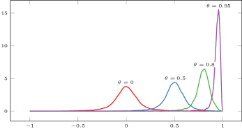
In Figure 1, we plot the empirical density of the MLE for various values of $\theta$. We use the method in [23] for the simulation of the SBM, while the MLE associated to each trajectory is obtained maximizing numerically the log-likelihood. We see that the MLE is concentrated around the true value. The more $\theta$ is closer to $1$, the more the density is skewed to the left. In the next section we examine this behavior. For reasons related to symmetry, for the remainder of the document, we restrict to consider the case $\theta\geq 0$.

Refer to caption
Figure 1: Density of the MLE for various values of $\theta$ using $10\,000$ samples of the SBM using $\Delta t=10^{-4}$ for $T=1$.

1.1 Asymptotic mixed normality of the MLE estimator

We establish, in the forthcoming Theorem 1, the asymptotic mixed normality of the MLE, with the non standard rate of $n^{1/4}$. This result has already been proven, when $\theta=0$, in [21]. Before to state the result, let us first introduce a definition specifying the nature of the asymptotic normality.

Definition 1 (Class of $\mathcal{L}$-mixed normal distribution).

Let $L_{1}$ be the local time at point 00 and time $1$ of the SBM $X$ and $G\sim\mathcal{N}(0,1)$ be independent from $\mathcal{F}_{1}$ (hence from $L_{1}$). Note that the distribution of $L_{1}$ does not depend on $\theta$. A random variable $M$ is said to be $\mathcal{L}$-mixed normal distributed if

$$M\stackrel{{\scriptstyle\mathrm{law}}}{{=}}\frac{G}{\sqrt{L}_{1}}.$$

Note that a $\mathcal{L}$-mixed normal distribution has an infinite second moment. It is a symmetric, unimodal distribution with heavy tails.

Remark 3 (Simulation of the local time).

The local time of the SBM is equal in distribution to the one of the Brownian motion, hence $L_{1}\stackrel{{\scriptstyle\mathrm{law}}}{{=}}|H|$ for $H\sim\mathcal{N}(0,1)$. Therefore, the local time and $\mathcal{L}$-mixed normal distributions are easily simulated.

Remark 4 (Scaling).

Let $L$ be the symmetric local time of a SBM $X$ at the point 00 and $W$ be a Brownian motion $W$ independent from $X$. They both satisfy a scaling property, in particular for the local time it holds $L_{T}\stackrel{{\scriptstyle\mathrm{law}}}{{=}}\sqrt{T}L_{1}$. Hence,

$$\frac{W(L_{T})}{L_{T}}\stackrel{{\scriptstyle\mathrm{law}}}{{=}}\frac{W(1)}{\sqrt{L_{T}}}\stackrel{{\scriptstyle\mathrm{law}}}{{=}}\frac{W(1)}{T^{1/4}\sqrt{L_{1}}}.$$

In other words, $T^{1/4}W(L_{T})/L_{T}$ and $T^{1/4}G/\sqrt{L_{1}}$ (for $G\sim\mathcal{N}(0,1)$ independent from $X$) are $\mathcal{L}$-mixed normal distributed.

We also introduce a quantity related to the asymptotic variance of the estimator and to the Fisher information:

$$\mathcal{s}(\theta):=\left(-\iint_{\mathbb{R}^{2}}\mu_{\theta}(x)p_{\theta}(1,x,y)\partial_{\theta}k(x,y)\,\mathrm{d}x\,\mathrm{d}y\right)^{\!-1/2}\in\mathbb{R}.$$ (3)

The quantity $\mathcal{s}(\theta)$ will be studied in more details in Proposition 2, Remark 5, and in Section 3, in particular in Section 3.3.

We are now ready to state the main result which says that $(nT)^{1/4}\mathcal{s}(\theta)^{-1}(\theta_{n}-\theta)$ is asymptotically a $\mathcal{L}$-mixed normal distribution under $\mathbb{P}_{\theta}$.

Theorem 1 (Asymptotic $\mathcal{L}$-mixed normality of the MLE for the SBM).

Let $\theta\in(-1,1)$. The MLE estimator $\theta_{n}$ is asymptotically mixed normal with

$$n^{1/4}(\theta_{n}-\theta)\xrightarrow[n\to\infty]{\text{stably}}\mathcal{s}(\theta)\frac{H}{\sqrt{L_{T}}},\text{ under }\mathbb{P}_{\theta},$$

where $H\sim\mathcal{N}(0,1)$ independent from $\mathcal{F}_{T}$ (hence of $L_{T}$).

The proof of Theorem 1 follows from the results of the next section, Section 1.2, which rely on the study of the score and its derivatives that we propose in Section 2.

Heuristically, the non standard rate of $n^{1/4}$, can be explained by the fact that the quality of the estimation depends mainly on the time spent by the SBM around 00, and that the fraction of observations when $\{X_{t_{i}}\}_{i=0,\dotsc,n}$ is of order $\sqrt{n}$. This fact is rigorously established for the Skew Random Walk where the local time is really the occupation time at the point where the bias-dynamic is perturbed [19].

Although it was conjectured in [22] from the results on the Skew Random Walk that the coefficient $\mathcal{s}(\theta)$ in front of the mixed Gaussian should be proportional to $\sqrt{1-\theta^{2}}$, we find a slowly varying pre-factor.

Proposition 2.

For all $\theta\in(-1,1)$, the function $(x,y)\mapsto\mu_{\theta}(x)p_{\theta}(1,x,y)\partial_{\theta}k(x,y)$ is integrable and its integral is negative, so $\mathcal{s}(\theta)\in(0,\infty)$ is well defined. Besides there exist two real constants $0<c_{1}\leq c_{2}<\infty$ such that for all $\theta\in(-1,1)$

$$c_{-}\sqrt{1-\theta^{2}}\leq\mathcal{s}(\theta)\leq c_{+}\sqrt{1-\theta^{2}}.$$

We find that $0.79\leq c_{-}<c_{+}\leq 0.88$, which is consistent with the numerical observations of [22].

The proof of Proposition 2 is provided in Section 3.3 where a more precise statement is formulated. Actually we show in Remark 14 that an accurate approximation of $\mathcal{s}(\theta)$ is given by

$$\mathcal{s}(\theta)\approx\frac{\sqrt{1-\theta^{2}}}{\sqrt{1.292+0.232\,\theta^{2}+0.071\,\theta^{4}}}.$$

1.2 Asymptotic expansion for the MLE estimator

Let us first consider the following family of statistics of interest:

$\displaystyle\mathsf{S}_{m}(n,\theta):=\frac{1}{n^{1/2}}\sum_{i=0}^{\lfloor nT\rfloor-1}\partial_{\theta}^{m}k_{\theta}(X_{t_{i}}\sqrt{n},X_{t_{i+1}}\sqrt{n})\text{ for }m\geq 0.$ (4)

Remark 2 shows that $\mathsf{S}_{m}(n,\theta)=\partial_{\theta}^{m}\left(\partial_{\theta}\log\Lambda_{n}(\theta)\right)/n^{1/2}$ so that $\mathsf{S}_{m}(n,/\theta)$ is the renormalized $m$-th order derivative of the score.

Let us also consider the statistics, on $\{\mathsf{S}_{1}(n,\theta)\neq 0\}$,

$\displaystyle\mathsf{d}_{k,n}(\theta):=\frac{-1}{k!}\frac{\mathsf{S}_{k}(n,\theta)}{\mathsf{S}_{1}(n,\theta)}\text{ for }k\geq 0\quad\text{ and }\quad\mathsf{P}_{n}(\theta):=n^{1/4}\frac{T^{1/4}}{\mathcal{s}(\theta)}\mathsf{d}_{0,n}(\theta),$

as well as the constants

$$\xi_{m}(\theta):=\iint_{\mathbb{R}^{2}}\mu_{\theta}(x)p_{\theta}(1,x,y)\partial_{\theta}^{m}k(x,y)\,\mathrm{d}x\,\mathrm{d}y,\quad\text{ for }m\in\mathbb{N}.$$ (5)

The integrability of $(x,y)\mapsto\mu_{\theta}(x)p_{\theta}(1,x,y)\partial_{\theta}^{m}k(x,y)$ is shown in Section 3, together with other properties of $\xi_{m}(\theta)$.

Remark 5.

The quantity $\mathcal{s}(\theta)$ given by (3) is related to $\xi_{1}(\theta)$: $\mathcal{s}(\theta)^{-2}=-\xi_{1}(\theta)$.

Proposition 3.

Under $\mathbb{P}_{\theta}$,

  1. 1.

    the statistics $\mathsf{P}_{n}(\theta)=n^{1/4}T^{1/4}\mathsf{d}_{0,n}(\theta)/\mathcal{s}(\theta)$ is asymptotically $\mathcal{L}$-mixed normal distributed;

  2. 2.

    for every $k\geq 1$,

    $$\mathsf{d}_{k,n}(\theta)\xrightarrow[n\to\infty]{\text{prob.}}\mathsf{d}_{k}(\theta):=\frac{-\xi_{k}(\theta)}{k!\xi_{1}(\theta)}=\frac{\mathcal{s}(\theta)^{2}}{k!}\xi_{k}(\theta).$$ (6)

Moreover, under $\mathbb{P}_{0}$, for every $k\geq 1$, $\mathsf{d}_{2k,n}(0)\xrightarrow[n\to\infty]{\text{prob.}}0$ and $\mathsf{d}_{2k}(0)$ is, up to a multiplicative constant, $\mathcal{L}$-mixed normal distributed. Furthermore $\{n^{1/4}\mathsf{d}_{2k,n}(0)\}_{k=0,\dotsc,m}$ converges stably for any $m\geq 1$. The limit is identified in Proposition 4 in Section 2.

Proof.

This is an immediate consequence of Proposition 4 in Section 2 on the asymptotic behavior of the score combined with Remark 5. ∎

In Theorem 2, we give an expansion of the MLE in term of $\mathsf{d}_{0,n}(\theta)$ (and so of $\frac{\mathcal{s}(\theta)\mathsf{P}_{n}(\theta)}{T^{1/4}n^{1/4}}$). It follows from applying Theorem 3 in [20]. For $\theta=0$, such a type of expansion was already given in [21] in the form provided in equation (8) below. We also provide an alternative expansion based on a finer analysis of the coefficients’ asymptotic behavior.

Let us introduce some notation: for any $m\in\mathbb{N}\cup\{\infty\}$, let

$$\Phi^{[m]}(\delta,x):=\sum_{k=1}^{m}\delta_{k}x^{k}$$ (7)

be the formal power series in $x$ of coefficients $\delta=\{\delta_{k}\}_{k\geq 1}$.

Theorem 2 (Asymptotic expansion, cf. [20, Theorem 3]).

For any integer $n\geq 1$, any $N\geq 1$, and any $\theta\in(-1,1)$, the MLE satisfies under $\mathbb{P}_{\theta}$,

$$\theta_{n}=\theta+\Phi^{[\infty]}(\mathsf{D}_{\cdot,n}(\theta),\mathsf{d}_{0,n}(\theta))=\theta+\sum_{k=1}^{+\infty}\mathsf{D}_{k,n}(\theta)\mathsf{d}_{0,n}(\theta)^{k},$$ (8)

where $\mathsf{D}_{1,n}(\theta):=1$ and $\mathsf{D}_{q,n}(\theta)$, $q=2,\ldots,N$, are given by the following recursive formula:

$$\mathsf{D}_{q,n}(\theta):=\sum_{m=2}^{q}\mathsf{d}_{m,n}(\theta)\sum_{k_{1}+\dotsb+k_{m}=q}\mathsf{D}_{k_{1},n}(\theta)\dotsb\mathsf{D}_{k_{m},n}(\theta).$$ (9)

If $\theta=0$, another expansion holds

$$\theta_{n}=\Phi^{[\infty]}(\mathsf{a}_{\cdot,n},n^{-1/4})=\mathsf{d}_{0,n}(0)+\sum_{\begin{subarray}{c}k\geq 3\\ k\text{ odd}\end{subarray}}\frac{\mathsf{a}_{k,n}}{n^{k/4}},$$ (10)

where $\mathsf{a}_{k,n}$ for $k=0,\ldots,N$ is $\mathsf{a}_{2q,n}:=0$ if $q\geq 0$, and

$$\displaystyle\mathsf{a}_{1,n}:=n^{1/4}\mathsf{d}_{0,n}(0)=\mathcal{s}(0)\mathsf{P}_{n}(0)/{T^{1/4}},$$
$$\displaystyle\begin{multlined}\mathsf{a}_{2q+1,n}:=\sum_{\begin{subarray}{c}m=2\\ m\text{ even }\end{subarray}}^{2q}n^{1/4}\mathsf{d}_{m,n}(0)\sum_{k_{1}+\dotsb+k_{m}=2q}\mathsf{a}_{k_{1},n}\cdots\mathsf{a}_{k_{m},n}\\ +\sum_{\begin{subarray}{c}m=3\\ m\text{ odd }\end{subarray}}^{2q+1}\mathsf{d}_{m,n}(0)\sum_{k_{1}+\dotsb+k_{m}=2q+1}\mathsf{a}_{k_{1},n}\cdots\mathsf{a}_{k_{m},n}.\end{multlined}\mathsf{a}_{2q+1,n}:=\sum_{\begin{subarray}{c}m=2\\ m\text{ even }\end{subarray}}^{2q}n^{1/4}\mathsf{d}_{m,n}(0)\sum_{k_{1}+\dotsb+k_{m}=2q}\mathsf{a}_{k_{1},n}\cdots\mathsf{a}_{k_{m},n}\\ +\sum_{\begin{subarray}{c}m=3\\ m\text{ odd }\end{subarray}}^{2q+1}\mathsf{d}_{m,n}(0)\sum_{k_{1}+\dotsb+k_{m}=2q+1}\mathsf{a}_{k_{1},n}\cdots\mathsf{a}_{k_{m},n}.$$
Remark 6.

From [20], it can be seen that $\Phi(\mathsf{d}_{\cdot,n}(\theta),\Phi(\mathsf{D}_{\cdot,n}(\theta),x))=-x$. For the first coefficients, it holds

$$\displaystyle\mathsf{D}_{2,n}=\mathsf{d}_{2,n},\ \mathsf{D}_{3,n}=\mathsf{d}_{3,n}+2\mathsf{d}_{2,n}^{2},$$
$$\displaystyle\mathsf{D}_{4,n}=\mathsf{d}_{4,n}+5\mathsf{d}_{2,n}\mathsf{d}_{3,n}+5\mathsf{d}_{2,n}^{3}$$
$$\displaystyle\text{and }\mathsf{D}_{5,n}=\mathsf{d}_{5,n}+6\mathsf{d}_{2,n}\mathsf{d}_{4,n}+21\mathsf{d}_{2,n}^{2}\mathsf{d}_{3,n}+14\mathsf{d}_{2,n}^{4}+3\mathsf{d}_{3,n}^{2}.$$

In the case of the sequence in (10),

$$\displaystyle\mathsf{a}_{3,n}=\mathsf{d}_{3,n}(0)\mathsf{P}_{n}(0)^{3}\mathcal{s}(0)^{3}/T^{3/4}+n^{1/4}\mathsf{d}_{2,n}(0)\mathsf{P}_{n}(0)^{2}\mathcal{s}(0)^{2}/T^{1/2}$$
 $$\displaystyle\text{ and }\mathsf{a}_{5,n}=(\mathsf{d}_{5,n}(0)+3\left(\mathsf{d}_{3,n}(0)\right)^{2})\mathsf{P}_{n}(0)^{5}\mathcal{s}(0)^{5}/T^{5/4}$$
$$\displaystyle+(5n^{1/4}\mathsf{d}_{2,n}(0)\mathsf{d}_{3,n}(0)+n^{1/4}\mathsf{d}_{4,n}(0))\mathsf{P}_{n}(0)^{4}\mathcal{s}(0)^{4}/T$$
$$\displaystyle+2n^{1/2}\left(\mathsf{d}_{2,n}(0)\right)^{2}\mathsf{P}_{n}(0)^{3}\mathcal{s}(0)^{3}/T^{3/4}.$$
Remark 7.

As $\mathsf{d}_{k,n}$ and $\mathsf{P}_{n}$ depend on $\theta$, they cannot be computed under the true parameter in the context of estimation (actually, $\mathsf{P}_{n}(\theta_{n})=0=\mathsf{d}_{0,n}(\theta_{n})$ for the MLE $\theta_{n}$) but can be used for statistical hypothesis testing.

The result shows a sort of “phase transition” between $\theta=0$ and $\theta\neq 0$. This is clearly related to the dichotomy in the convergence of $\mathsf{d}_{2m,n}(0)$ (vanishing) and $n^{1/4}\mathsf{d}_{2m,n}(0)$ for $m\geq 1$: Observe, for instance, that the second term in equation (10) is of order $1/n^{3/4}$ and in equation (8) is of order $1/n^{1/2}$. This latter term, in the case $\theta=0$ goes to 0 as $n$ increases.

Theorem 2 and Proposition 3 prove Theorem 1. Moreover they imply, for all $m\in\mathbb{N}$, approximations of the MLE given by the formal power series

$${\theta}_{n}^{[m]}:=\theta+\Phi^{[m]}(\mathsf{D}_{\cdot,n}(\theta),\mathsf{d}_{0,n}(\theta))\quad\text{and}\quad\check{\theta}_{n}^{[m]}:=\theta+\Phi^{[m]}(\mathsf{D}_{\cdot}(\theta),\mathsf{d}_{0,n}(\theta)),$$ (11)

where $\mathsf{D}_{k}(\theta)$ is defined similarly to $\mathsf{D}_{k,n}(\theta)$ in (9) with $\mathsf{d}_{k,n}$ replaced by $\mathsf{d}_{n}$ in (6). More precisely, $\mathsf{D}_{1}(\theta):=1$ and for $q=2,\ldots,N$, $\mathsf{D}_{q}$ is given by the recursive formula:

$$\mathsf{D}_{q}(\theta):=\sum_{m=2}^{q}\mathsf{d}_{m}(\theta)\sum_{k_{1}+\dotsb+k_{m}=q}\mathsf{D}_{k_{1}}(\theta)\dotsb\mathsf{D}_{k_{m}}(\theta).$$ (12)

Then, for instance,

$$\check{\theta}_{n}^{[3]}=\theta+\mathsf{d}_{0,n}-\frac{1}{2}\frac{\xi_{2}(\theta)}{\xi_{1}(\theta)}\left(\mathsf{d}_{0,n}\right)^{2}+\frac{1}{2}\left(\left(\frac{\xi_{2}(\theta)}{\xi_{1}(\theta)}\right)^{2}-\frac{\xi_{3}(\theta)}{3\xi_{1}(\theta)}\right)\left(\mathsf{d}_{0,n}\right)^{3}.$$

The power series $\theta_{n}^{[m]}$ is the $m$-th order truncation of (8). It has random coefficients $\mathsf{D}_{\cdot,n}(\theta)$ and random argument $\mathsf{d}_{0,n}(\theta)$ involving the score and its derivatives. The proxy $\check{\theta}_{n}^{[m]}$ is a power series with deterministic coefficients $\mathsf{D}_{\cdot}(\theta)$ (limit of $\mathsf{D}_{\cdot,n}(\theta)$) and the same random argument $\mathsf{d}_{0,n}(\theta)$ related to the score and its first derivative. Both $\theta_{n}^{[m]}$ and $\check{\theta}_{n}^{[m]}$ are non-linear expressions of $\mathsf{d}_{0,n}(\theta)$.

The following result enlightens the coefficients’ behavior as $\theta$ varies in $(-1,1)$. It is proved in Section 3.
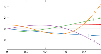
Lemma 1.

Let $\{\xi_{m}\}_{m\in\mathbb{N}}$ defined in (5). Then for all $m\in\mathbb{N}$:

  1. 1.

    $\xi_{0}\equiv 0$;

  2. 2.

    $\theta\mapsto\xi_{2m+1}(\theta)$ is even;

  3. 3.

    There exists $-\infty<c_{m,1}<c_{m,2}<0$ such that $-c_{m,1}\leq(1-\theta^{2})^{2m+1}\xi_{2m+1}(\theta)\leq c_{m,2}$ for all $\theta\in(-1,1)$;

  4. 4.

    $\xi_{2m}(\theta)$ is odd, in particular $\xi_{2m}(0)=0$;

  5. 5.

    There exists $c_{2m}\in(0,\infty)$ such that $-c_{2m}\leq(1-\theta^{2})^{2m}\xi_{2m}(\theta)<0$ for all $\theta\in(0,1)$.

The following result is proved by induction on the recursive formula (9).

Corollary 1 (of Proposition 3 and Lemma 1).

It holds that

$$\mathsf{D}_{k,n}(\theta)\xrightarrow[n\to\infty]{\text{prob.}}\mathsf{D}_{k}(\theta).$$

Besides, for any $k\geq 1$,

$$|\mathsf{D}_{k}(\theta)\mathcal{s}(\theta)^{k}|\leq\frac{C_{k}}{(1-\theta^{2})^{k/2-1}}$$

for a constant $C_{k}\geq 0$.

We plot the coefficients $\theta\mapsto\mathsf{D}_{k}(\theta)\mathcal{s}(\theta)^{k}$ in Figure 2, up to this scaling factor $\theta\mapsto(1-\theta^{2})^{1-k/2}$.

Refer to caption
Figure 2: Functions $\theta\mapsto\mathsf{D}_{k}(\theta)\mathcal{s}(\theta)^{k}(1-\theta^{2})^{k/2-1}$ with $\mathsf{D}_{k}$ defined by (12) for $\theta$ restricted to $[0,1]$ and $m=1,\dotsc,5$.
Remark 8.

The coefficients $\mathsf{D}_{k,n}(\theta)$ converge towards their limits at rate of $n^{1/4}$. This is a consequence of definition (9) and Proposition 3.
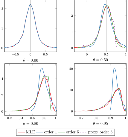
Refer to caption
Figure 3: Density of MLE, $\theta_{n}^{[1]}=\theta+\mathsf{d}_{0,n}(\theta)$, and the fifth order expansions $\theta_{n}^{[5]}$ and $\check{\theta}_{n}^{[5]}$ (11), for several values of $\theta$ using $10\,000$ samples of the SBM using $\Delta t=10^{-3}$ for $T=1$ (thus, $n=1000$).

In Figure 3 we show the empirical densities of the MLE $\theta_{n}$, $\theta_{n}^{[1]}=\theta+\mathsf{d}_{0,n}(\theta)$, $\theta_{n}^{[5]}$, and of the proxy $\check{\theta}_{n}^{[5]}$(see (11) for the definitions of $\theta_{n}^{[5]}$ and $\check{\theta}_{n}^{[5]}$). For $\theta=0$, $\mathsf{d}_{0,n}(0)$ replicates already very well the MLE behavior, therefore there $\theta_{n}^{[5]}$ and $\check{\theta}_{n}^{[5]}$ are not plotted. For $\theta\neq 0$, we observe that, while the lower order expansions replicate worse the MLE behavior, $\theta_{n}^{[5]}$ and $\check{\theta}_{n}^{[5]}$ do it quite well, and so do the higher order expansions. The expansions $\theta_{n}^{[5]}$ and $\check{\theta}_{n}^{[5]}$ are close one to another. Indeed they are respectively random and deterministic polynomials of $\mathsf{d}_{0,n}(\theta)$ such that, by Corollary 1, the random coefficients converge to the deterministic ones. To introduce the next paragraph, observe that the density of $\theta_{n}^{[1]}=\theta+\mathsf{d}_{0,n}(\theta)$ is skewed to the left when $\theta$ is close to $1$. Of course, since their density is close to the one of the MLE’s, $\theta_{n}^{[5]}$ and $\check{\theta}_{n}^{[5]}$ exhibit a skewed empirical distribution.

Remark 9.

Let us remind that as for $\theta_{n}-\theta$, $n^{1/4}\mathsf{d}_{0,n}(\theta)$ has asymptotic symmetric distribution: Proposition 3 ensures that $n^{1/4}\mathsf{d}_{0,n}(\theta)=\mathsf{P}_{n}(\theta)\mathcal{s}(\theta)T^{-1/4}$ is asymptotically $\mathcal{L}$-mixed normal distributed. Therefore the alternative proxys $\Phi^{[m]}(\mathsf{D}_{\cdot}(\theta),\mathsf{P}_{\infty}(\theta)\mathcal{s}(\theta)(nT)^{-1/4})$ where $\mathsf{P}_{\infty}$ follows a $\mathcal{L}$-mixed normal distribution, would not replicate skewness and they would need higher order expansions than the proxys $\check{\theta}^{[m]}_{n}$ in order to have empirical distribution which gets close to the MLE’s one.

Skewness.

We have observed skewness for the empirical distribution $\mathsf{d}_{0,n}(\theta)$ and of the MLE. This is due to the fact that the empirical density of the score shows that the more $\theta$ is close to $1$ the more the score is skewed to the left. However, the correlation between MLE and score is non-trivial : non-linear dependence. The approximations of the MLE in (11) are non-linear functions of the score and its derivative, actually of $\mathsf{d}_{0,n}$ which is basically their ratio. Since $\mathsf{D}_{2}(\theta)=\mathsf{d}_{2}(\theta)=-\frac{1}{2}\frac{\xi_{2}(\theta)}{\xi_{1}(\theta)}$, Lemma 1 establishes that $\operatorname{sgn}(\mathsf{D}_{2}(\theta))=-\operatorname{sgn}(\theta)$. This favors a skewness to the left (resp. right) when $\theta>0$ (resp. $\theta<0$) of the distribution of the proxys (11). In other words, the approximations of the MLE proposed above capture the skewness of the MLE.

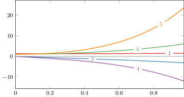
Boundary layer effect.

Let us set

$$f_{m}(\theta):=\frac{(-1)^{m}(1-\theta^{2})^{m}}{m!}\xi_{m}(\theta).$$ (13)
Refer to caption
Figure 4: Functions $\theta\mapsto f_{m}(\theta)$ defined by (13) for $\theta$ restricted to $[0,1]$ and $m=1,\dotsc,5$.

Then $f_{2k+1}$ is positive and bounded (from above and below by a positive constant), $f_{2k}(0)=0$ and $f_{2k}(\theta)$ is bounded. Then, (11) rewrites:

$$\check{\theta}^{[3]}_{n}=\theta+\frac{\sqrt{1-\theta^{2}}}{\sqrt{f_{1}(\theta)}}\frac{\mathsf{P}_{n}(\theta)}{(Tn)^{1/4}}+\frac{f_{2}(\theta)}{f_{1}(\theta)^{2}}\left(\frac{\mathsf{P}_{n}(\theta)}{(Tn)^{1/4}}\right)^{2}\\ +\frac{1}{\sqrt{1-\theta^{2}}}\frac{2(f_{2}(\theta))^{2}-f_{3}(\theta)f_{1}(\theta)}{f_{1}(\theta)^{7/2}}\left(\frac{\mathsf{P}_{n}(\theta)}{(Tn)^{1/4}}\right)^{3},$$

that is

$\displaystyle\mathsf{D}_{1}(\theta)\mathcal{s}(\theta)$ $\displaystyle=\frac{\sqrt{1-\theta^{2}}}{\sqrt{f_{1}(\theta)}},\quad\mathsf{D}_{2}(\theta)\mathcal{s}(\theta)^{2}=\frac{f_{2}(\theta)}{f_{1}(\theta)^{2}}$
$\displaystyle\text{ and }\mathsf{D}_{3}(\theta)\mathcal{s}(\theta)^{3}$ $\displaystyle=\frac{1}{\sqrt{1-\theta^{2}}}\frac{2f_{2}(\theta)^{2}-f_{3}(\theta)f_{1}(\theta)}{f_{1}(\theta)^{7/2}}.$

The term of order $2$ vanishes for $\theta=0$ as $f_{2}(0)=0$. With this expansion, one sees a “boundary layer” effect for $|\theta|$ close to $1$ in the explosion of the third order coefficient. Indeed if we push the expansion up to order $k$ (here we stopped at $k=3$), the corresponding coefficient explodes as $(1-\theta^{2})^{(k-2)/2}$ when $|\theta|$ is close to $1$. We have performed numerical simulations that suggest that no cancellation effect occurs so that the approximation by a polynomial expansion is no longer suitable.

In [20] we discussed a similar boundary layer phenomenon in the case of the Binomial family. One could expect the same to happen for the skewness parameter $\theta$ because of the pathwise construction of SBM done associating independent Bernoulli random variables with parameter $(1+\theta)/2$ to the excursions from 0 of a reflected Brownian motion and flipping each excursion based on the result of the Bernoulli random variable.

Change of variable and change of coordinates.

Combining the Faà di Bruno formula with (8), one may given some explicit expansion of $\varphi(\theta_{n})$ for any analytic function $\varphi$. Similarly, one may also consider $\theta_{n}$ in another system of coordinates, as discussed in [20]. On that point, two changes of variables appear to be natural: $\varphi_{1}(\theta)=\sqrt{1-\theta^{2}}$ and $\varphi_{1}(\theta)=1/\sqrt{1-\theta^{2}}$. The latter one stabilizes the variance. However, no change of coordinate impacts the asymptotic behavior of the score. Besides, we found through numerical experiments that using $\varphi_{1}$ or $\varphi_{2}$ does not improve Wald confidence intervals.

2 Asymptotic behavior of the score and its derivatives

In this section, we provide results which are necessary to prove Proposition 3. These results are an application of the results in [14] for the Brownian motion, and on the ones from [22] (convergence) and [27] (Central Limit Theorem) for the (true) SBM.

Let us recall that $\mathsf{S}_{m}$ in (4) is nothing else that a rescaled derivative of the score and $\xi_{m}(\theta)$ is a constant defined in (5). By Lemma 1, it holds that for all $\theta\in(-1,1)$, $\xi_{0}(\theta)=0$ and $\xi_{1}(\theta)$ is negative, and that for all integer $m$, $\xi_{2m}(0)=0$.

Proposition 4.

For any $\theta\in(-1,1)$, the family $\{\xi_{k}(\theta)\}_{k\geq 0}$ defined by (5) is such that:

  1. 1.

    Under $\mathbb{P}_{\theta}$, there exists a standard (with mean 00 and variance $1$) Gaussian random variable $H$ independent from $\mathcal{F}_{T}$ (the probability space $(\Omega,\mathcal{F},\mathbb{P}_{0})$ has been extended to carry $H$) such that for any $m\geq 0$,

    $\displaystyle n^{1/4}\mathsf{S}_{0}(n,\theta)\xrightarrow[n\to\infty]{\text{stably}}\sqrt{-\xi_{1}(\theta)}\sqrt{L_{T}}H,$
    $\displaystyle(\mathsf{S}_{1}(n,\theta),\dotsc,\mathsf{S}_{m}(n,\theta))\xrightarrow[n\to\infty]{\text{prob.}}(\xi_{1}(\theta)L_{T},\dotsc,\xi_{m}(\theta)L_{T}).$

    Thanks to the property of the stable convergence, we have joint stable convergence of $(n^{1/4}\mathsf{S}_{0}(n,\theta),\mathsf{S}_{1}(n,\theta),\dotsc,\mathsf{S}_{m}(n,\theta))$.

  2. 2.

    For $\theta=0$ (the SBM is actually a Brownian motion), under $\mathbb{P}_{0}$, there exists a Gaussian family $H=\{H_{k}\}_{k=0,\dotsc,m}$ independent from $\mathcal{F}_{T}$ with mean 00 and covariance $\operatorname{Cov}(H_{j},H_{\ell})=\Psi_{2j,2\ell}$ for $0\leq j,\ell\leq m$ described in Section 3.5 (the probability space $(\Omega,\mathcal{F},\mathbb{P}_{0})$ has been extended to carry $H$) such that for any $m\geq 0$,

    $\displaystyle\{n^{1/4}\mathsf{S}_{2k}(n,0)\}_{k=0,\dotsc,m}\xrightarrow[n\to\infty]{\text{stably}}\{\sqrt{L_{T}}H_{k}\}_{k=0,\dotsc,m},$
    $\displaystyle\{\mathsf{S}_{2k+1}(n,0)\}_{k=0,\dotsc,m}\xrightarrow[n\to\infty]{\text{prob.}}\{\xi_{2k+1}(0)L_{T}\}_{k=0,\dotsc,m}.$

    Thanks to the property of the stable convergence, we have joint stable convergence of $(n^{1/4}\mathsf{S}_{0}(n,\theta),\mathsf{S}_{1}(n,\theta),n^{1/4}\mathsf{S}_{2}(n,\theta),\dotsc)$.

Remark 10.

Following [14, 27], a stronger result holds: on an extended probability space, there exist a $m$-dimensional Brownian motion $\{W_{k}\}_{k\geq 0}$ independent from $L$ and a $m\times m$-matrix $\Xi(\theta)$ such that

$$\left\{\frac{1}{n^{1/4}}\left(\frac{1}{\sqrt{n}}\sum_{i=1}^{\lfloor nt\rfloor}\partial^{\ell}k_{\theta}(X_{i-1}\sqrt{n},X_{i}\sqrt{n})-\xi_{\ell}(\theta)L_{t}\right)\right\}_{\ell=0,\dotsc,m,\ t\in[0,T]}\\ \xrightarrow[n\to\infty]{\text{stably}}\{\Xi(\theta)W(L_{t})\}_{t\in[0,T]}.$$ (14)

A closed-form — yet cumbersome — expression exists for the matrix $\Xi(\theta)=\left(\Xi_{i,j}(\theta)\right)_{i,j=0,\ldots,m}$. Here, we focus on the particular cases $m=0$ and $\theta=0$ and we study $\{\xi_{k}(\theta)\}_{k=1,\dotsc,\max(m,1)}$ and $\Xi$ for these cases.

Remark 11.

When $\xi_{m}(\theta)=0$, (14) rewrites

$$n^{1/4}\mathsf{S}_{m}(n,\theta)\xrightarrow[n\to\infty]{\text{stably}}\Xi_{m,m}(\theta)\sqrt{L_{T}}G$$

for some constant $\Xi_{m,m}(\theta)$, and $G\sim\mathcal{N}(0,1)$ independent of $L_{T}$. In particular,

  1. 1.

    For any $\theta\in(-1,1)$ and $m=0$,

    $$\Xi_{0,0}(\theta)=\sqrt{-\xi_{1}(\theta)}=\frac{1}{\mathcal{s}(\theta)}.$$

    This follows from [27] and Lemma 4.

  2. 2.

    For $\theta=0$, $\Xi(0)\Xi(0)^{\mathrm{T}}=\Psi$ for $\Psi$ appearing in Proposition 4.2 and discussed in Section 3.5.

Statistical implications.

The convergence results of Proposition 4 are the key for the convergence of the MLE in Theorem 1. Besides, we could also use these results to construct

  • estimators of the local time using $\mathsf{S}_{1}(n,\theta_{n})/\xi_{1}(\theta_{n})$;

  • Wald confidence interval using $\mathcal{s}(\theta_{n})$ as a substitute for $\mathcal{s}(\theta)$;

  • hypothesis testing on the true value of $\theta$ using either a confidence interval around $\theta$, or $\mathsf{S}_{0}(n,\theta)^{2}/\mathsf{S}_{1}(n,\theta)$ which behaves asymptotically as a $\chi^{2}_{1}$ distribution.

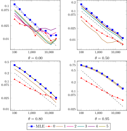
2.1 Rate of convergence

In this section, we estimate numerically the rate of convergence towards the the limit distribution of the score. More precisely, we study empirically the rate convergence of $\mathsf{S}_{k}(n,\theta)$ in (4) towards its limit. In particular, we show that the speeds deteriorates as $|\theta|$ becomes close to $1$.

We plot in Figure 5 the Kolmogorov-Smirnov distance $\Delta_{\mathrm{KS}}(n)$ between the empirical distributions

  1. (a)

    of $\mathcal{s}(\theta)^{-1}n^{1/4}(\theta_{n}-\theta)$ and $H/\sqrt{L_{T}}$ with $H\sim\mathcal{N}(0,1)$, independent from the local time.

  2. (b)

    of $\mathsf{S}_{k}(n,\theta)/\Xi_{k,k}(\theta)$ and $\sqrt{L_{T}}H$ with $H\sim\mathcal{N}(0,1)$, independent from the local time, for $k=0$ or for $\theta=0$ and $k$ even.

  3. (c)

    of $\mathsf{S}_{k}(n,\theta)/\xi_{k}(\theta)$ and $L_{T}$ in other cases.

Refer to caption
Figure 5: Behavior of $n\mapsto\Delta_{\mathrm{KS}}(n)$ using $10\,000$ samples of the SBM with $T=1$, and comparison with $C/\sqrt{n}$ (dashed line), in log-log scale, for statistics (a) (MLE), (b) (00 for any $\theta$ and $2,4$ if $\theta=0$) and (c) in the other cases.

Even for small moderate values of the sample size $n$, the asymptotic regime is reached most of the case. The 5 %-quantile of the Kolmogorov-Smirnov statistics is $0.52$ while the 1 %-quantile is $0.44$.

In each case, the statistics $\Delta_{\mathrm{KS}}(n)$ behaves like $C/n^{\eta}$, with $\eta$ close to $1/2$.

For the score of order 00 or when $\theta$ is close to $1$, the rate $\eta$ is lower than $1/2$. The constant $C$ is greater for the MLE than for the other Kolmogorov-Smirnov statistics. In each case, the constant increases with $\theta$, as well as the ratio between the constant $C$ for the MLE and the one for the score of order 00.

Note that we are close to the Berry-Esseen rate even though our sample is not composed of independent identically distributed random variables.

In Figure 5, when the Kolmogorov-Smirnov distances are small and $n$ is big, the plotted distance is affected by the Monte-Carlo error. For $\theta=0$, the terms of order $2$ and $4$ in the expansion of the MLE (8) vanish. The asymptotic law of these coefficients is the one given in (b). Note that, in the alternative expansion of the MLE (10), the terms of odd order of the latter expansion involve the statistics in (b) and (c). For $\theta\neq 0$, the effect of the terms of orders $k\geq 2$ in the expansion (8), which behave asymptotically as $(1-\theta^{2})^{1-k/2}$, have some increasing effect on the MLE.

3 The limiting coefficients

Our aim is to study the limiting coefficients $\mathcal{s}(\theta)$ in (3), $\xi_{m}(\theta)$ in (5) and $\Psi$ appearing in Proposition 4. We also prove Proposition 2 and Lemma 1. We actually establish additional properties useful in numerical studies and applications. For instance, in Section 3.4, we provide an expansion of $\theta\mapsto\xi_{m}(\theta)$ around 0. In Section 3.5, we study the matrix $\Psi$ in Proposition 4.2.

3.1 The coefficients $\xi_{k}$

We study up to Section 3.4 the limiting coefficients $\xi_{k}$.

We take profit from the explicit expression of the density, hence of $k_{\theta}$. We conveniently rewrite

$$k_{\theta}(x,y):=\begin{cases}\dfrac{1}{\theta+\exp(2xy)}&\text{ if }x\geq 0,\ y\geq 0,\\ \dfrac{1}{\exp(2xy)-\theta}&\text{ if }x\leq 0,\ y\leq 0,\\ \dfrac{1}{\theta-1}&\text{ if }x\geq 0,\ y\leq 0,\\ \dfrac{1}{1+\theta}&\text{ if }x\leq 0,\ y\geq 0.\end{cases}$$
Lemma 2.

For any $m\geq 0$,

$$\partial_{\theta}^{m}k_{\theta}(x,y)=m!(-1)^{m}k_{\theta}^{m+1}(x,y)$$ (15)

for any $x,y\in\mathbb{R}$.

Proof.

Let us note first that

$$\partial_{\theta}k_{\theta}(x,y)=\frac{-\operatorname{sgn}(y)^{2}}{(\operatorname{sgn}(y)\theta+\exp(2(xy)^{+}))^{2}}=\frac{-1}{(\operatorname{sgn}(y)\theta+\exp(2(xy)^{+}))^{2}}\\ =-k_{\theta}(x,y)^{2}.$$ (16)

Thus, (15) is true for $m=0,1$. Let us assume that (15) is true for some $m\geq 1$. With (16),

$$\partial_{\theta}^{m+1}k_{\theta}(x,y)=(-1)^{m}m!\partial_{\theta}(k_{\theta}(x,y)^{m+1})\\ =(-1)^{m}(m+1)!\partial_{\theta}k_{\theta}(x,y)\cdot k_{\theta}(x,y)^{m}=(-1)^{m+1}(m+1)!k_{\theta}(x,y)^{m+2}.$$

This proves that (15) is true for $m+1$, and thus for any $m$. ∎

Notation 1.

We define for some integer $m\geq 1$,

$\displaystyle\chi^{\pm\pm}_{m}(\theta):=\iint_{\mathbb{R}^{2}}\mathbf{1}_{\pm x\geq 0,\pm y\geq 0}k_{\theta}(x,y)^{m}p_{\theta}(1,x,y)\mu_{\theta}(x)\,\mathrm{d}x\,\mathrm{d}y,$ (17)
$\displaystyle\text{and }\chi_{m}(\theta):=\chi_{m}^{++}(\theta)+\chi_{m}^{--}(\theta)+\chi^{+-}_{m}(\theta)+\chi^{-+}_{m}(\theta).$ (18)

With Lemma 2, the coefficients $\xi_{m}$’s given by (5) are related to the $\chi_{m}$’s by

$$\xi_{m}(\theta)=m!(-1)^{m}\chi_{m+1}(\theta).$$ (19)

We now study $\chi_{m}(\theta)$ for $\theta\in(-1,1)$ and various values of $m$.

We note the relations

$\displaystyle p_{\theta}(1,-x,-y)$ $\displaystyle=p_{-\theta}(1,x,y),$ (20)
$\displaystyle k_{\theta}(-x,-y)$ $\displaystyle=-k_{-\theta}(x,y)$ (21)
$\displaystyle\text{and }\mu_{\theta}(-x)$ $\displaystyle=\mu_{-\theta}(x).$ (22)

A direct consequence of the symmetry relations (20)-(22) is the following lemma

Lemma 3 (Symmetry relation).

For any $m\geq 1$ and any $\theta\in(-1,1)$,

$$\displaystyle\chi^{--}_{m}(\theta)=(-1)^{m}\chi^{++}_{m}(-\theta)\text{ and }\chi^{-+}_{m}(\theta)=(-1)^{m}\chi^{+-}_{m}(-\theta).$$ (23)
Corollary 2.

For any $\theta\in(-1,1)$ and any $m\geq 1$,

  1. 1.

    $\theta\mapsto\chi_{2m}(\theta)$ is even and $\chi_{2m}(\theta)>0$.

  2. 2.

    $\theta\mapsto\chi_{2m+1}(\theta)$ is odd; in particular $\chi_{2m+1}(0)=0$ (we will see below in Lemma 7 that $\chi_{2m+1}(\theta)<0$ for any $\theta\in(0,1)$).

Proof.

Consequence of Lemma 3 and for proving $\chi_{2m}(\theta)>0$ one just observes the positivity of the integrands of equation (17). ∎

Lemma 4 (Values for $m=1$).

For any $\theta\in(-1,1)$, $\chi_{1}(\theta)=0$.

Proof.

This stems from the very definition of $k_{\theta}$ and the fact that $\int_{-\infty}^{+\infty}p_{\theta}(1,x,y)\,\mathrm{d}y=1$ so that $\partial_{\theta}\int_{-\infty}^{+\infty}p_{\theta}(1,x,y)\,\mathrm{d}y=0$. In fact,

$$\chi_{1}(\theta)=\int_{\mathbb{R}}\mathbb{E}_{\theta}[k_{\theta}(X_{0},X_{1})\nonscript\>|\nonscript\>\mathopen{}\allowbreak X_{0}=x]\mu_{\theta}(x)\,\mathrm{d}x$$

and for all $x\in\mathbb{R}$

$$\mathbb{E}_{\theta}[k_{\theta}(X_{0},X_{1})\nonscript\>|\nonscript\>\mathopen{}\allowbreak X_{0}=x]=\int_{\mathbb{R}}\frac{\partial_{\partial}p_{\theta}(1,x,y)}{p_{\theta}(1,x,y)}p_{\theta}(1,x,y)\,\mathrm{d}y=0.$$ (24)

Hence $\chi_{1}(\theta)=0$. ∎

Computation for $m\geq 2$.

The case $m\geq 2$ and $\theta>0$ is a bit more cumbersome.

Lemma 5.

For $m\geq 2$, $\theta\in(-1,1)$,

$$\chi^{+-}_{m}(\theta)=\frac{(-1)^{m}}{\sqrt{2\pi}}\frac{1+\theta}{(1-\theta)^{m-1}}\text{ and }\chi^{-+}_{m}(\theta)=\frac{1}{\sqrt{2\pi}}\frac{1-\theta}{(1+\theta)^{m-1}}.$$ (25)
Proof.

First,

$$\frac{1}{\sqrt{2\pi}}\iint_{\mathbb{R}^{2}}\mathbf{1}_{x\geq 0,y\geq 0}\exp\left(\frac{-(x+y)^{2}}{2}\right)\,\mathrm{d}x\,\mathrm{d}y=\int_{0}^{+\infty}\overline{\Phi}(z)\,\mathrm{d}z=\frac{1}{\sqrt{2\pi}}$$

with $\overline{\Phi}(x):=\frac{1}{\sqrt{2\pi}}\int_{x}^{+\infty}e^{-y^{2}/2}\,\mathrm{d}y$, the complementary distribution function of the unit, centered Gaussian random variable.

Hence,

$$\chi^{+-}_{m}(\theta)=\iint_{\mathbb{R}^{2}}\mathbf{1}_{x\geq 0,y\leq 0}k_{\theta}(x,y)^{m}p_{\theta}(1,x,y)\mu_{\theta}(x)\,\mathrm{d}x\,\mathrm{d}y=\frac{-(1+\theta)}{(1-\theta)^{m-1}}\int_{0}^{+\infty}\overline{\Phi}(x)\,\mathrm{d}x.$$

The value of $\chi_{m}^{-+}$ follows from (23). ∎

We express

$$\chi^{++}_{m}(\theta)=\iint_{\mathbb{R}^{2}}\mathbf{1}_{x\geq 0,y\geq 0}k_{\theta}(x,y)^{m}p_{\theta}(1,x,y)\mu_{\theta}(x)\,\mathrm{d}x\,\mathrm{d}y\\ =\iint_{\mathbb{R}^{2}}\mathbf{1}_{x\geq 0,y\geq 0}\frac{1}{\sqrt{2\pi}}(1+\theta)\frac{\exp\left(\frac{-(x-y)^{2}}{2}\right)}{(\theta+\exp(2xy))^{m}}\,\mathrm{d}x\,\mathrm{d}y\\ +\iint_{\mathbb{R}^{2}}\mathbf{1}_{x\geq 0,y\geq 0}\frac{1}{\sqrt{2\pi}}\theta(1+\theta)\frac{\exp\left(\frac{-(x+y)^{2}}{2}\right)}{(\theta+\exp(2xy))^{m}}\,\mathrm{d}x\,\mathrm{d}y\\ =\iint_{\mathbb{R}^{2}}\mathbf{1}_{x\geq 0,y\geq 0}\frac{1+\theta}{\sqrt{2\pi}}\exp\left(\frac{-(x+y)^{2}}{2}\right)\frac{1}{(\theta+\exp(2xy))^{m-1}}\,\mathrm{d}x\,\mathrm{d}y.$$ (26)

We could also use the following form

$$\chi^{++}_{m}(\theta)=\iint_{\mathbb{R}^{2}}\mathbf{1}_{x\geq 0,y\geq 0}\frac{1+\theta}{\sqrt{2\pi}}\exp\left(\frac{-x^{2}-y^{2}}{2}\right)\frac{\exp(xy)+\theta\exp(-xy)}{(\theta+\exp(2xy))^{m}}\,\mathrm{d}x\,\mathrm{d}y$$ (27)

which is suitable for Monte Carlo simulation as

$$\chi^{++}_{m}(\theta)=\frac{\sqrt{2\pi}}{4}(1+\theta)\mathbb{E}\left[\frac{\exp(|G\cdot G^{\prime}|)+\theta\exp(-|G\cdot G^{\prime}|)}{(\theta+\exp(2|G\cdot G^{\prime}|))^{m}}\right]$$ (28)

for two independent Gaussian, unit, centered random variables $G$ and $G^{\prime}$.

Remark 12.

The considerations in the remainder of this section or in Lemma 1 (which we are proving in this section), suggest to consider the equivalent expression

$$\chi^{++}_{m}(\theta)=\frac{\sqrt{2\pi}}{4(1-\theta)^{m}}(1+\theta)\mathbb{E}\left[(1-\theta)^{m}\frac{\exp(|G\cdot G^{\prime}|)+\theta\exp(-|G\cdot G^{\prime}|)}{(\theta+\exp(2|G\cdot G^{\prime}|))^{m}}\right]$$

which reduces the variance of the empirical mean without burdening the computational cost.

We consider first a close-form formula for the integral involved in $\chi^{++}_{m}(0)$.

Lemma 6 (Some values at $\theta=0$).

Let $m\geq 2$, then

$$\sqrt{2\pi}\chi^{++}_{m}(0)=\frac{1}{2\sqrt{m(m-1)}}\log\left(2m-1+2\sqrt{m(m-1)}\right)\in(0,1).$$

In particular, when $m$ is large, $\sqrt{2\pi}\chi^{++}_{m}(0)\sim\log(4m)/2m$.

Remark 13.

We could also write $\chi^{++}_{m}(0)=\frac{1}{2\sqrt{m(m-1)}}\operatorname{atanh}\frac{2\sqrt{m(m-1)}}{2m-1}$.

Proof of Lemma 6.

From (26) we see that $\sqrt{2\pi}\chi^{++}_{m}(0)=\alpha_{2m-1}$ where

$$\alpha_{n}:=\int_{0}^{+\infty}\int_{0}^{+\infty}\exp\left(\frac{-x^{2}-y^{2}}{2}-nxy\right)\,\mathrm{d}x\,\mathrm{d}y$$

for $n\geq 1$. Let $n\geq 2$ be fixed. Using the change of variable $(x,y)=(\sqrt{v\log(u)},\sqrt{\log(u)/v})$ for $u\geq 1$, $v\geq 0$, we obtain that

$$\alpha_{n}=\int_{0}^{+\infty}\int_{1}^{+\infty}\frac{1}{2vu}\frac{1}{u^{n+v/2+1/2v}}\,\mathrm{d}u\,\mathrm{d}v=\int_{0}^{+\infty}\frac{1}{v^{2}+2nv+1}\,\mathrm{d}v.$$

Since $n\geq 2$, from (3.3.17) in [1], this leads

$$\alpha_{n}=\frac{1}{2\sqrt{n^{2}-1}}\log\frac{n+\sqrt{n^{2}-1}}{n-\sqrt{n^{2}-1}}=\frac{1}{\sqrt{n^{2}-1}}\log(n+\sqrt{n^{2}-1})\in(0,1)$$

which can be also written as $\frac{1}{\sqrt{n^{2}-1}}\operatorname{atanh}\frac{\sqrt{n^{2}-1}}{n}$. ∎

The following inequalities are consequences of (26). For all $\theta\in[0,1)$, $m\geq 2$:

$$\pm\frac{1}{\sqrt{2\pi}}\frac{1}{(1\pm\theta)^{m-2}}\sqrt{2\pi}\chi^{++}_{m}(0)\leq\pm\chi^{++}_{m}(\pm\theta)\leq\pm\frac{1\pm\theta}{\sqrt{2\pi}}\sqrt{2\pi}\chi^{++}_{m}(0).$$ (29)
Lemma 7.

For any $m\geq 1$ and $\theta\in(-1,1)$ with $\theta\neq 0$, then $\xi_{m}(\theta)\neq 0$.

Proof.

Equality (19) and Corollary 2 ensure that it suffices to prove that $(0,1)\ni\theta\mapsto\chi_{2m+1}(\theta)<0$. Let $m\geq 1$ and $\theta\in(0,1)$ be fixed.

Equations (23), the explicit expression for $\chi^{-+}_{2m+1}(\theta)$ in (25), the upper inequality in (29) and the fact that $\sqrt{2\pi}\chi^{++}_{2m+1}(0)<1$ (see Lemma 6) yield

$$\begin{split}\chi_{2m+1}(\theta)&=\chi^{++}_{2m+1}(\theta)-\chi^{++}_{2m+1}(-\theta)+\chi^{+-}_{2m+1}(\theta)-\chi^{+-}_{2m+1}(-\theta)\\ &\leq\frac{1}{\sqrt{2\pi}}\left(2\theta\sqrt{2\pi}\chi^{++}_{2m+1}(0)-\frac{1+\theta}{(1-\theta)^{2m}}+\frac{1-\theta}{(1+\theta)^{2m}}\right)\\ &<\frac{1}{\sqrt{2\pi}}\left(2\theta-\frac{1+\theta}{(1-\theta)^{2m}}+\frac{1-\theta}{(1-\theta)^{2m}}\right)=\frac{2\theta}{\sqrt{2\pi}}\left(1-\frac{1}{(1-\theta)^{2m}}\right)<0.\end{split}$$

This proves that $\xi_{m}(\theta)$ does not vanish for $\theta\neq 0$. ∎

We are now ready to provide the proof of Lemma 1. The proof of Proposition 2 is also provided and requires studying $\chi_{2}(\theta)=-\xi_{1}(\theta)=\mathcal{s}(\theta)^{-2}$.

3.2 Proof of Lemma 1

As (19) relates $\xi$ and $\chi$, Item 1 in Lemma 1 follows from Lemma 4. Item 2 and 4 are Corollary 2. We now prove Items 3 and 5. Actually we provide a finer result.

For every $\theta\in(-1,1)$ and $k\geq 1$, by (23) and (25), it holds

$$\begin{split}\frac{\xi_{2m}(\theta)}{(2m)!}&=\chi_{2m+1}(\theta)=\chi^{++}_{2m+1}(\theta)-\chi^{++}_{2m+1}(-\theta)+\chi^{+-}_{2m+1}(\theta)-\chi^{+-}_{2m+1}(-\theta)\\ &=\chi^{++}_{2m+1}(\theta)-\chi^{++}_{2m+1}(-\theta)+\frac{1}{\sqrt{2\pi}}\frac{(1+\theta)^{2m+1}-(1-\theta)^{2m+1}}{(1-\theta^{2})^{2m}}\end{split}$$

and

$$\begin{split}-\frac{\xi_{2m-1}(\theta)}{(2m-1)!}&=\chi_{2m}(\theta)=\chi^{++}_{2m}(\theta)+\chi^{++}_{2m}(-\theta)+\chi^{+-}_{2m}(\theta)+\chi^{+-}_{2m}(-\theta)\\ &=\chi^{++}_{2m}(\theta)+\chi^{++}_{2m}(-\theta)+\frac{1}{\sqrt{2\pi}}\frac{1+\theta}{(1-\theta)^{2m}}+\frac{1}{\sqrt{2\pi}}\frac{1-\theta}{(1+\theta)^{2m}}.\end{split}$$

In the proof of Lemma 7 we have already obtained a bound. We find finer ones. Let us recall the bound here: for every $\theta\in(0,1)$

$$\begin{split}\frac{\xi_{2m}(\theta)}{(2m)!}&=\chi_{2m+1}(\theta)<-\frac{2\theta}{\sqrt{2\pi}}\left(\frac{1}{(1-\theta)^{2m}}-1\right).\end{split}$$

Similarly as in the proof of Lemma 7 we can obtain the desired bounds, by combining inequalities (29) and Lemma 6. For every $\theta\in(0,1)$ we get

$$\displaystyle\begin{split}\frac{\xi_{2m}(\theta)}{(2m)!}&\geq-\frac{1+\sqrt{2\pi}\chi^{++}_{2m+1}(0)}{\sqrt{2\pi}}\left(\frac{1}{(1-\theta)^{2m}}-\frac{1}{(1+\theta)^{2m}}\right)\\ &\qquad-\theta\frac{1-\sqrt{2\pi}\chi^{++}_{2m+1}(0)}{\sqrt{2\pi}}\left(\frac{1}{(1-\theta)^{2m}}+\frac{1}{(1+\theta)^{2m}}\right)\\ &\geq-\frac{2}{\sqrt{2\pi}}\left(\frac{1}{(1-\theta)^{2m}}+\frac{1}{(1+\theta)^{2m}}\right)>-\frac{4}{\sqrt{2\pi}}\frac{1}{(1-\theta)^{2m}};\end{split}$$ (30)
$$\displaystyle\begin{split}-\frac{\xi_{2m-1}(\theta)}{(2m-1)!}&=\chi_{2m}(\theta)\leq\chi^{++}_{2m}(0)\left(1+\theta+\frac{1}{(1-\theta)^{2(m-1)}}\right)\\ &\qquad+\frac{1}{\sqrt{2\pi}}\frac{1+\theta}{(1-\theta)^{2m-1}}+\frac{1}{\sqrt{2\pi}}\frac{1-\theta}{(1+\theta)^{2m-1}},\end{split}$$ (31)

and

$$\begin{split}-\frac{\xi_{2m-1}(\theta)}{(2m-1)!}&\geq\chi^{++}_{2m}(0)\left(1-\theta+\frac{1}{(1+\theta)^{2(m-1)}}\right)\\ &\qquad+\frac{1}{\sqrt{2\pi}}\frac{1+\theta}{(1-\theta)^{2m-1}}+\frac{1}{\sqrt{2\pi}}\frac{1-\theta}{(1+\theta)^{2m-1}}.\end{split}$$ (32)

We conclude that for all $\theta\in(-1,1)$,

$$-\frac{4}{\sqrt{2\pi}}\frac{1}{(1-|\theta|)^{2m-1}}<\frac{\xi_{2m-1}(\theta)}{(2m-1)!}<-\frac{1+|\theta|}{\sqrt{2\pi}}\frac{1}{(1-|\theta|)^{2m-1}}$$

as well as

$$\begin{split}&-\frac{4}{\sqrt{2\pi}}\frac{1}{(1-|\theta|)^{2m}}<\frac{\xi_{2m}(|\theta|)}{(2m)!}<-\frac{2|\theta|}{\sqrt{2\pi}}\left(\frac{1}{(1-|\theta|)^{2m}}-1\right)\leq 0,\\ &0\leq\frac{2|\theta|}{\sqrt{2\pi}}\left(\frac{1}{(1-|\theta|)^{2m}}-1\right)<\frac{\xi_{2m}(-|\theta|)}{(2m)!}<\frac{4}{\sqrt{2\pi}}\frac{1}{(1-|\theta|)^{2m}}.\end{split}$$

These inequalities imply Items 3 and 5 of Lemma 1 and complete its proof.

3.3 Proof of Proposition 2

We prove Proposition 2 which completes the analysis of the asymptotic mixed normality in Theorem 1.

The proof of Lemma 1, in particular (31)-(32), show that for all $\theta$,

$$-\frac{2}{\sqrt{2\pi}}\frac{1+\theta^{2}}{1-\theta^{2}}-\chi^{++}_{2}(0)(2+|\theta|)<\xi_{1}(\theta)<-\frac{2}{\sqrt{2\pi}}\frac{1+\theta^{2}}{1-\theta^{2}}-\chi^{++}_{2}(0)(2-|\theta|),$$

where $\chi^{++}_{2}(0)\approx 0.62$ by Lemma 6. This would already prove Proposition 2, but the next lemma allow us to establish better bounds.

Lemma 8.

Let

$$\mathcal{I}(\theta):=\int_{0}^{\infty}\int_{0}^{\infty}\frac{(1-e^{-2xy})}{(1-\theta^{2}e^{-4xy})}e^{-4xy-\frac{(x+y)^{2}}{2}}\,\mathrm{d}x\,\mathrm{d}y.$$

Then $\mathcal{I}$ is increasing on $[0,1]$ and $\mathcal{I}(\theta)\in[\mathcal{I}(0),\mathcal{I}(1)]$ where

$\displaystyle\mathcal{I}(0)$ $\displaystyle=\sqrt{2\pi}(\chi^{++}_{3}(0)-\chi^{++}_{4}(0))\approx 0.088,$
$\displaystyle\mathcal{I}(1)$ $\displaystyle=\int_{0}^{\infty}\int_{0}^{\infty}\frac{1}{(1+e^{-2xy})}e^{-4xy-\frac{(x+y)^{2}}{2}}\,\mathrm{d}x\,\mathrm{d}y\in[\sqrt{2\pi}\chi^{++}_{3}(0)/2,\sqrt{2\pi}\chi^{++}_{4}(0)],$

and

$$\mathcal{s}(\theta)^{-2}=-\xi_{1}(\theta)=\chi_{2}(\theta)=\frac{2}{\sqrt{2\pi}}\left(\frac{1+\theta^{2}}{1-\theta^{2}}+\sqrt{2\pi}\chi^{++}_{2}(0)-\theta^{2}\mathcal{I}(\theta)\right).$$ (33)

Recall that Lemma 6 shows that $\sqrt{2\pi}\chi^{++}_{2}(0)\approx 0.62$, $\sqrt{2\pi}\chi^{++}_{3}(0)/2\approx 0.24$, and $\sqrt{2\pi}\chi^{++}_{4}(0)\approx 0.38.$

Proof.

First note that $[-1,1]\ni\theta\mapsto\mathcal{I}(\theta)$ is an even function and increasing on $[0,1]$, therefore the first part of the statement follows from (26) and Lemma 6. We have already obtained the expressions (25) and (27) hence

$$\chi_{2}(\theta)=\frac{1}{\sqrt{2\pi}}\frac{1+\theta^{2}}{1-\theta^{2}}\\ +\int_{0}^{\infty}\int_{0}^{\infty}\frac{(1+\theta)(1-\theta e^{-2xy})+(1-\theta)(1+\theta e^{-2xy})}{(1-\theta^{2}e^{-4xy})}{e^{-2xy}}e^{-\frac{(x+y)^{2}}{2}}\,\mathrm{d}y\,\mathrm{d}x.$$

We rewrite the integrand in a suitable way

$$\begin{split}\chi_{2}(\theta)&=\frac{1}{\sqrt{2\pi}}\frac{1+\theta^{2}}{1-\theta^{2}}+\frac{2}{\sqrt{2\pi}}\int_{0}^{\infty}\int_{0}^{\infty}\frac{(1-\theta^{2}e^{-2xy})}{(1-\theta^{2}e^{-4xy})}{e^{-2xy}}e^{-\frac{(x+y)^{2}}{2}}\,\mathrm{d}y\,\mathrm{d}x\\ &=\frac{1}{\sqrt{2\pi}}\frac{1+\theta^{2}}{1-\theta^{2}}+\frac{2}{\sqrt{2\pi}}\int_{0}^{\infty}\int_{0}^{\infty}\left(1-\frac{\theta^{2}e^{-2xy}(1-e^{-2xy})}{(1-\theta^{2}e^{-4xy})}\right){e^{-2xy}}e^{-\frac{(x+y)^{2}}{2}}\,\mathrm{d}y\,\mathrm{d}x,\end{split}$$

where we recognize the right-hand-side of (33). ∎

Remark 14.

We have obtained the following bounds for $\chi_{2}(\theta)=-\xi_{1}(\theta)=\mathcal{s}(\theta)^{-2}$: By (33),

$$\frac{2}{\sqrt{2\pi}}\frac{1+\theta^{2}}{1-\theta^{2}}+2\chi^{++}_{2}(0)-\frac{2}{\sqrt{2\pi}}\theta^{2}\mathcal{I}(0)\leq\chi_{2}(\theta)\leq\frac{2}{\sqrt{2\pi}}\frac{1+\theta^{2}}{1-\theta^{2}}+2\chi^{++}_{2}(0)-\frac{2}{\sqrt{2\pi}}\theta^{2}\mathcal{I}(1).$$

Since $\mathcal{I}(0)=\sqrt{2\pi}(\chi^{++}_{3}(0)-\chi^{++}_{4}(0))\approx 0.088$ and $\mathcal{I}(1)\leq\sqrt{2\pi}\chi^{++}_{4}(0)$, by studying the bounds above which are functions of $\theta$, we can show that

$$\frac{\mathcal{s}(\theta)}{\sqrt{1-\theta^{2}}}\in[0.79,0.88].$$

Numerically, we found that $\mathcal{s}(\theta)$ is pretty close to its upper bound.

3.4 Expansion around 0

We provide a polynomial expansion around 00 of $\theta\mapsto\xi_{m}(\theta)$. By (19), it suffices to provide it for $\theta\mapsto\chi_{m}(\theta)$. Since we could not compute explicitly $\xi_{m}(\theta)$, this expansion allows us to compute it using their value at $\theta=0$ given in Lemma 6. Let us also recall that we could rewrite $\chi_{m}(\theta)$ in a form suitable for Monte Carlo simulation, see (28).

Let us define

$$\zeta_{m}(\theta):=\chi_{m}^{++}(\theta)+\chi_{m}^{+-}(\theta)-\chi_{m}^{--}(\theta)-\chi_{m}^{-+}(\theta).$$

Using the symmetry relations (20)-(22), $\theta\mapsto\zeta_{2m}(\theta)$ is odd, while $\theta\mapsto\zeta_{2m+1}(\theta)$ is even. In particular, $\zeta_{2m}(0)=0$.

Besides,

$$\chi_{2m}(0)=\beta_{2m}\text{ and }\zeta_{2m+1}(0)=\beta_{2m+1}$$

with

$$\beta_{m}:=\sqrt{\frac{2}{\pi}}\left(\sqrt{2\pi}\chi^{++}_{m}(0)+(-1)^{m}\right)$$

and $\chi^{++}_{m}(0)$ provided in Lemma 6.

Lemma 9.

For any $m\geq 1$,

$\displaystyle\partial_{\theta}\chi_{m}(\theta)$ $\displaystyle=-(m-1)\chi_{m+1}(\theta)+\zeta_{m}(\theta),$ (34)
$\displaystyle\partial_{\theta}\zeta_{m}(\theta)$ $\displaystyle=-(m-1)\zeta_{m+1}(\theta)+\chi_{m}(\theta).$ (35)
Proof.

Differentiating with respect to $\theta$,

$$\partial_{\theta}\chi^{\pm\pm}_{m}(\theta)=m\iint_{\mathbb{R}^{2}}\mathbf{1}_{\pm x\geq 0,\pm y\geq 0}\partial_{\theta}k_{\theta}(x,y)k_{\theta}(x,y)^{m-1}p_{\theta}(1,x,y)\mu_{\theta}(x)\,\mathrm{d}x\,\mathrm{d}y\\ +\iint_{\mathbb{R}^{2}}\mathbf{1}_{\pm x\geq 0,\pm y\geq 0}k_{\theta}(x,y)^{m}\frac{\partial_{\theta}p_{\theta}(1,x,y)}{p_{\theta}(1,x,y)}p_{\theta}(1,x,y)\mu_{\theta}(x)\,\mathrm{d}x\,\mathrm{d}y\\ +\iint_{\mathbb{R}^{2}}\mathbf{1}_{\pm x\geq 0,\pm y\geq 0}\operatorname{sgn}(x)k_{\theta}(x,y)^{m}p_{\theta}(1,x,y)\,\mathrm{d}x\,\mathrm{d}y.$$

With (15) and since $k_{\theta}(x,y)=\partial_{\theta}p_{\theta}(1,x,y)/p_{\theta}(1,x,y)$,

$$\partial_{\theta}\chi^{\pm\pm}_{m}(\theta)=-m\iint_{\mathbb{R}^{2}}\mathbf{1}_{\pm x\geq 0,\pm y\geq 0}\mu_{\theta}(x)k_{\theta}(x,y)^{m+1}p_{\theta}(1,x,y)\,\mathrm{d}x\,\mathrm{d}y\\ +\iint_{\mathbb{R}^{2}}\mathbf{1}_{\pm x\geq 0,\pm y\geq 0}\mu_{\theta}(x)k_{\theta}(x,y)^{m+1}p_{\theta}(1,x,y)\,\mathrm{d}x\,\mathrm{d}y\\ +\iint_{\mathbb{R}^{2}}\mathbf{1}_{\pm x\geq 0,\pm y\geq 0}\operatorname{sgn}(x)k_{\theta}(x,y)^{m}p_{\theta}(1,x,y)\,\mathrm{d}x\,\mathrm{d}y.$$

We then obtain

$\displaystyle\partial_{\theta}\chi^{++}_{m}(\theta)$ $\displaystyle=-(m-1)\chi^{++}_{m+1}(\theta)+\chi^{++}_{m}(\theta),$
$\displaystyle\partial_{\theta}\chi^{+-}_{m}(\theta)$ $\displaystyle=-(m-1)\chi^{+-}_{m+1}(\theta)+\chi^{+-}_{m}(\theta),$
$\displaystyle\partial_{\theta}\chi^{-+}_{m}(\theta)$ $\displaystyle=-(m-1)\chi^{-+}_{m+1}(\theta)-\chi^{-+}_{m}(\theta),$
$\displaystyle\partial_{\theta}\chi^{--}_{m}(\theta)$ $\displaystyle=-(m-1)\chi^{--}_{m+1}(\theta)-\chi^{--}_{m}(\theta).$

With these four expressions, we obtain easily (34) and (35). ∎

Corollary 3.

For $k\geq 1$ and $m\geq 1$,

$$\partial^{k}_{\theta}\chi_{m}(\theta)=\sum_{\ell=0}^{k}(-1)^{\ell}b_{\ell}\binom{k}{\ell}\Big{(}\chi_{m+\ell}(\theta)a_{\ell}+\zeta_{m+\ell}(\theta)(1-a_{\ell})\Big{)}$$ (36)

with

$$a_{\ell}=\begin{cases}1&\text{ if }k-\ell\text{ is even},\\ 0&\text{ if }k-\ell\text{ is odd}\end{cases}\text{ and }b_{\ell}=\begin{cases}1&\text{ if }\ell=0,\\ (m-1)\dotsb(m-\ell-2)&\text{ if }\ell\geq 1.\end{cases}.$$
Proof.

We form the formal power series in $\mathbb{R}[[\lambda,\mu]]$ for unknown $\lambda$ and $\mu$ by

$$X(\theta)=\sum_{m\geq 1}\lambda^{m}\chi_{m}(\theta)+\sum_{m\geq 1}\mu^{m}\zeta_{m}(\theta).$$

We then define two linear operators $S$ and $J$ on $\mathbb{R}[[\lambda,\mu]]$ defined by $S(\nu^{m+1})=-(m-1)\nu^{m}$ for $\nu=\lambda,\nu$ and $J(\lambda^{m})=\mu^{m}$, $J(\mu^{m})=\lambda^{m}$ so that $J$ exchanges $\mu$ and $\lambda$ and $J^{2}$ is idempotent. The operators $S$ and $J$ commute. With our choice of $S$,

$$S(X(\theta))=-\sum_{m\geq 1}(m-1)\lambda^{m}\chi_{m+1}(\theta)-\sum_{m\geq 1}\mu^{m}\zeta_{m+1}(\theta),$$

so that we write (34)-(35) as

$$\partial_{\theta}X(\theta)=(S+J)X(\theta).$$

Therefore,

$$\partial^{k}_{\theta}X(\theta)=\sum_{\ell=0}^{k}\binom{k}{\ell}S^{\ell}J^{k-\ell}X(\theta).$$

We then deduce (36). ∎

From (36),

$\displaystyle\partial^{2}_{\theta}\chi_{m}(\theta)$ $\displaystyle=(m-1)m\chi_{m+2}(\theta)-2(m-1)\zeta_{m+1}(\theta)+\chi_{m}(\theta),$
$\displaystyle\partial^{3}_{\theta}\chi_{m}(\theta)$ $\displaystyle=-(m-1)m(m+1)\chi_{m+3}(\theta)+3(m-1)m\zeta_{m+2}(\theta)-3(m-1)\chi_{m+1}+\zeta_{m}(\theta).$

The Taylor expansion around 00 leads to the following result.

Corollary 4.

For any $\theta$ with $|\theta|<1$, $\chi_{m}(\theta)=\chi_{m}(0)+\sum_{k\geq 1}c_{m,k}\theta^{k}$ where $c_{2m,1}=0$, $c_{2m+1,1}=-2m\chi_{2m+2}(0)$ and each of the $c_{m,k}$ is a linear superposition of values of $\beta_{\ell}$ for $\ell=m,\dotsc,\ell+k$.

In particular,

$$\chi_{2}(\theta)\approx 1.29+2.17\cdot\theta^{2}+\dotsb\text{ and }\chi_{3}(\theta)\approx-0.42\cdot\theta-2.93\cdot\theta^{2}+\dotsb.$$

3.5 The limiting covariance

We now show how to compute, at least numerically, the covariance matrix $\Psi$ appearing in Proposition 4.2. Recall that $\xi_{2i}(0)=0$ for any $i\geq 0$.

According to [14, Theorem 1.2, p. 511] or [27],

$$\Psi_{2i,2j}:=\int_{\mathbb{R}}\mathbb{E}\left[\left(\partial_{\theta}^{2i}k_{0}(B_{0},B_{1})\partial_{\theta}^{2j}k_{0}(B_{0},B_{1})\right)\nonscript\>\middle|\nonscript\>\mathopen{}\allowbreak B_{0}=x\right]\,\mathrm{d}x\\ +2\int_{\mathbb{R}}\mathbb{E}\left[\sum_{\ell\geq 1}\partial_{\theta}^{2i}k_{0}(B_{0},B_{1})\partial_{\theta}^{2j}k_{0}(B_{\ell},B_{\ell+1})\nonscript\>\middle|\nonscript\>\mathopen{}\allowbreak B_{0}=x\right]\,\mathrm{d}x,$$

for a Brownian motion $B$. Owing to (15) in Lemma 2,

$$\Psi_{2i,2j}=(2i)!(2j)!\int_{\mathbb{R}}\mathbb{E}\left[\sum_{\ell\leq 0}k_{0}^{2i+1}(B_{0},B_{1})k^{2j+1}_{0}(B_{\ell},B_{\ell+1})\nonscript\>\middle|\nonscript\>\mathopen{}\allowbreak B_{0}=x\right]\,\mathrm{d}x.$$

We decompose this expression as

$$\Psi_{2i,2j}=(2i)!(2j)!\left(\underline{\Psi}^{I}_{2i,2j}+\underline{\Psi}^{II}_{2i,2j}+\underline{\Psi}^{III}_{2i,2j}\right)$$

with

$\displaystyle\underline{\Psi}^{I}_{2i,2j}=$ $\displaystyle\int_{\mathbb{R}}\mathbb{E}\left[k_{0}^{2i+1}(B_{0},B_{1})k_{0}^{2j+1}(B_{0},B_{1})\nonscript\>\middle|\nonscript\>\mathopen{}\allowbreak B_{0}=x\right]\,\mathrm{d}x,$
$\displaystyle\underline{\Psi}^{II}_{2i,2j}=$ $\displaystyle\int_{\mathbb{R}}\mathbb{E}\left[k_{0}^{2i+1}(B_{0},B_{1})k^{2j+1}_{0}(B_{1},B_{2})\nonscript\>\middle|\nonscript\>\mathopen{}\allowbreak B_{0}=x\right]\,\mathrm{d}x$
$\displaystyle+\int_{\mathbb{R}}\mathbb{E}\left[k_{0}^{2j+1}(B_{0},B_{1})k^{2i+1}_{0}(B_{1},B_{2})\nonscript\>\middle|\nonscript\>\mathopen{}\allowbreak B_{0}=x\right]\,\mathrm{d}x,$
$\displaystyle\underline{\Psi}^{III}_{2i,2j}=$ $\displaystyle\int_{\mathbb{R}}\mathbb{E}\left[\sum_{\ell\geq 2}k_{0}^{2i+1}(B_{0},B_{1})k^{2j+1}_{0}(B_{\ell},B_{\ell+1})\nonscript\>\middle|\nonscript\>\mathopen{}\allowbreak B_{0}=x\right]\,\mathrm{d}x$
$\displaystyle+\int_{\mathbb{R}}\mathbb{E}\left[\sum_{\ell\geq 2}k_{0}^{2j+1}(B_{0},B_{1})k^{2i+1}_{0}(B_{\ell},B_{\ell+1})\nonscript\>\middle|\nonscript\>\mathopen{}\allowbreak B_{0}=x\right]\,\mathrm{d}x.$
Lemma 10.

It holds that

$$\underline{\Psi}_{2i,2j}^{I}=\chi_{2(i+j)+2}(0)=\frac{2}{\sqrt{2\pi}}\left(1+\sqrt{2\pi}\chi^{++}_{2(i+j+1)}(0)\right)=\frac{-\xi_{2(i+j)+1}(0)}{(2(i+j)+1)!}.$$ (37)

In particular, $\Xi_{0,0}(0)=\sqrt{\underline{\Psi}^{I}_{0,0}}=\sqrt{-\xi_{1}(0)}$.

Proof.

Eq. (37) follows from the definition of $\xi_{m}$ in (5) and (19). When $i=j=0$, by the Markov property and (24), we have $\underline{\Psi}^{II}_{0,0}=\underline{\Psi}^{III}_{0,0}=0$. ∎

By (18) and Lemma 5, $\chi_{2(i+j)+2}(0)=\frac{2}{\sqrt{2\pi}}(1+\sqrt{2\pi}\chi_{2(i+j)+2}^{++}(0))$, and an approximation of $\chi^{++}(0)$ is given in Lemma 6.

For $m\geq 1$, $m$ odd, we set

$\displaystyle\kappa_{m}(x,y)$ $\displaystyle:=\exp(-2m(xy)_{+})\operatorname{sgn}(y)=k_{0}(x,y)^{m}$
$\displaystyle\text{ and }\widehat{\kappa}_{m}(x,y)$ $\displaystyle:=\exp(-2m(xy)_{+})\operatorname{sgn}(x)=\kappa_{m}(y,x).$

We also define

$\displaystyle K_{m}(x)$ $\displaystyle:=\int\kappa_{m}(x)\exp\left(\frac{-(x-y)^{2}}{2}\right)\frac{\,\mathrm{d}y}{\sqrt{2\pi}}=\mathbb{E}[\kappa_{m}(x,B_{1})\nonscript\>|\nonscript\>\mathopen{}\allowbreak B_{0}=x]$
$\displaystyle\text{ and }\widehat{K}_{m}(x)$ $\displaystyle:=\int\widehat{\kappa}_{m}(x)\exp\left(\frac{-(x-y)^{2}}{2}\right)\frac{\,\mathrm{d}y}{\sqrt{2\pi}}=\mathbb{E}[\widehat{\kappa}_{m}(x,B_{1})\nonscript\>|\nonscript\>\mathopen{}\allowbreak B_{0}=x]$

for a Brownian motion $B$. With some straightforward computations,

$\displaystyle K_{m}(x)$ $\displaystyle=\operatorname{sgn}(x)\exp(2x^{2}m(m-1))\Phi(-(2m-1)|x|)-\operatorname{sgn}(x)\Phi(-|x|)$
$\displaystyle\text{ and }\widehat{K}_{m}(x)$ $\displaystyle=\operatorname{sgn}(x)\exp(2x^{2}m(m-1))\Phi(-(2m-1)|x|)+\operatorname{sgn}(x)\Phi(-|x|).$
Notation 2 ((Scaled) complementary error function).

The complementary error function and the scaled complementary error function are

$$\operatorname{erfc}(x):=\frac{2}{\sqrt{\pi}}\int_{x}^{+\infty}e^{-y^{2}}\,\mathrm{d}y=2\overline{\Phi}(x\sqrt{2})\text{ and }\operatorname{erfcx}(x):=\exp\left(x^{2}\right)\operatorname{erfc}(x)$$

for $x\geq 0$.

The functions $x\in[0,1]\mapsto\operatorname{erfc}(x)$ and $x\in[0,1]\mapsto\operatorname{erfcx}(x)$ take their values in $[0,1]$. Thanks to the Mill’s ratio, for $x$ large, $\operatorname{erfcx}(x)\sim 1/x\sqrt{\pi}$.

We also introduce

$$b_{m}:=\frac{2m-1}{\sqrt{2}}\text{ so that }2m(m-1)=b_{m}^{2}-\frac{1}{2}.$$

As $\Phi(-|x|)=\overline{\Phi}(|x|)$, we rewrite $K_{m}$ and $\widehat{K}_{m}$ as

$\displaystyle K_{m}(x)$ $\displaystyle=\frac{1}{2}\operatorname{sgn}(x)e^{-x^{2}/2}\left(\operatorname{erfcx}(b_{m}|x|)-\operatorname{erfcx}(|x|/\sqrt{2})\right)$
$\displaystyle\text{ and }\widehat{K}_{m}(x)$ $\displaystyle=\frac{1}{2}\operatorname{sgn}(x)e^{-x^{2}/2}\left(\operatorname{erfcx}(b_{m}|x|)+\operatorname{erfcx}(|x|/\sqrt{2})\right).$
Lemma 11.

For $i,j\geq 0$,

$$\underline{\Psi}^{III}_{2i,2j}=\sum_{\ell\geq 2}\frac{1}{\sqrt{2\pi}\sqrt{\ell-1}}\int_{-\infty}^{+\infty}\int_{-\infty}^{+\infty}\widehat{K}_{2i}(y)K_{2j}(z)\exp\left(\frac{-(z-y)^{2}}{2(\ell-1)}\right)\,\mathrm{d}y\,\mathrm{d}z\\ +\sum_{\ell\geq 2}\frac{1}{\sqrt{2\pi}\sqrt{\ell-1}}\int_{-\infty}^{+\infty}\int_{-\infty}^{+\infty}\widehat{K}_{2j}(y)K_{2i}(z)\exp\left(\frac{-(z-y)^{2}}{2(\ell-1)}\right)\,\mathrm{d}y\,\mathrm{d}z.$$
Proof.

We define for $m,n\geq 0$,

$$A(\ell,m,n):=\int_{-\infty}^{+\infty}\mathbb{E}[\kappa_{m}(B_{0},B_{1})\kappa_{n}(B_{\ell},B_{\ell+1})\nonscript\>|\nonscript\>\mathopen{}\allowbreak B_{0}=x]\,\mathrm{d}x$$ (38)

so that

$$\underline{\Psi}^{III}_{2i,2j}=\sum_{\ell\geq 2}2A(\ell,2i+1,2j+1).$$

We rewrite $A(\ell,m,n)$ using its integral form:

$$A(\ell,m,n)=\frac{1}{(2\pi)^{3/2}\sqrt{\ell-1}}\int_{-\infty}^{+\infty}\int_{-\infty}^{+\infty}\int_{-\infty}^{+\infty}\int_{-\infty}^{+\infty}\kappa_{m}(x,y)\kappa_{n}(z,u)\\ \times\exp\left(\frac{-(x-y)^{2}}{2}\right)\exp\left(\frac{-(z-y)^{2}}{2(\ell-1)}\right)\exp\left(\frac{-(z-u)^{2}}{2}\right)\,\mathrm{d}x\,\mathrm{d}y\,\mathrm{d}z\,\mathrm{d}u.$$ (39)

We compute first $A(\ell,m,n)$ for $\ell\geq 2$. Since $\widehat{\kappa}_{m}(y,x)=\kappa_{m}(x,y)$, inverting $x$ and $y$, and using the definitions of $K_{m}$ and $\widehat{K}_{m}$ leads to

$$A(\ell,m,n)=\frac{1}{\sqrt{2\pi}\sqrt{\ell-1}}\int_{-\infty}^{+\infty}\int_{-\infty}^{+\infty}\widehat{K}_{m}(y)K_{n}(z)\exp\left(\frac{-(z-y)^{2}}{2(\ell-1)}\right)\,\mathrm{d}y\,\mathrm{d}z.$$

This gives the result. ∎

Remark 15.

With a change of variable $(y,z)\to(y/\sqrt{j-1},z/\sqrt{j-1})$, for $A$ introduced in (38),

$$A(\ell,m,n)=\sqrt{2\pi}\sqrt{\ell-1}\int_{-\infty}^{+\infty}\int_{-\infty}^{+\infty}\widehat{K}_{m}(y\sqrt{\ell-1})K_{n}(z\sqrt{\ell-1})\exp(yz)\\ \times\exp\left(\frac{-z^{2}}{2}\right)\exp\left(\frac{-y^{2}}{2}\right)\frac{\,\mathrm{d}y}{\sqrt{2\pi}}\frac{\,\mathrm{d}z}{\sqrt{2\pi}}.$$

For two independent Gaussian random variables $G,G^{\prime}\sim\mathcal{N}(0,1)$, we may write

$$A(\ell,m,n)=\sqrt{2\pi}\sqrt{\ell-1}\mathbb{E}[K_{m}(G^{\prime}\sqrt{\ell-1})\widehat{K}_{n}(G\sqrt{\ell-1})\exp(G\cdot G^{\prime})],$$

where $G,G^{\prime}\sim\mathcal{N}(0,1)$ are independent. However, the variance is high so that Monte Carlo techniques are unstable here.

Lemma 12.

For $i,j\geq 1$,

$$\underline{\Psi}^{II}_{2i,2j}=\int_{0}^{+\infty}e^{-x^{2}}\operatorname{erfcx}(b_{2i+1}x)\operatorname{erfc}(b_{2j+1}x)\,\mathrm{d}x-\frac{2}{\sqrt{\pi}}\left(\sqrt{2}-1\right).$$
Proof.

As above,

$$A(1,m,n)=\int_{-\infty}^{+\infty}\widehat{K}_{m}(x)K_{n}(x)\,\mathrm{d}x\\ =\frac{1}{2}\int_{0}^{+\infty}e^{-x^{2}}\operatorname{erfcx}(b_{m}x)\operatorname{erfc}(b_{n}x)\,\mathrm{d}x-\frac{1}{2}\int_{0}^{+\infty}e^{-x^{2}}\operatorname{erfcx}(x/\sqrt{2})^{2}\,\mathrm{d}x.$$

The quantity $\underline{\Psi}_{2i,2j}^{III}$ is then

$$\underline{\Psi}_{2i,2j}^{II}=A(1,2i+1,2j+1)+A(1,2j+1,2i+1).$$

According to [29, 4.7.2],

$$\int_{0}^{+\infty}e^{-x^{2}}\operatorname{erfcx}\left(\frac{x}{\sqrt{2}}\right)^{2}\,\mathrm{d}x=\int_{0}^{+\infty}\operatorname{erfc}\left(\frac{x}{\sqrt{2}}\right)^{2}\,\mathrm{d}x=\frac{2}{\sqrt{\pi}}\left(\sqrt{2}-1\right)\approx 0.467.$$

No closed-form expression for $\int_{-\infty}^{+\infty}e^{-x^{2}}\operatorname{erfcx}(b_{m}x)\operatorname{erfc}(b_{n}x)\,\mathrm{d}x$ seems to exists. However, this integral is easy to compute numerically as there exists various implementation of $\operatorname{erfcx}$. This could be done through a quadrature method to compute the integral or using a Monte Carlo method as

$$\int_{0}^{+\infty}e^{-x^{2}}\operatorname{erfcx}(b_{m}x)\operatorname{erfc}(b_{n}x)\,\mathrm{d}x\\ =\frac{\sqrt{\pi}}{\sqrt{2m-1}}\mathbb{E}\left[\operatorname{erfcx}\left(\frac{\sqrt{2m-1}}{\sqrt{2}}|G|\right)\operatorname{erfcx}\left(\frac{\sqrt{2n-1}}{\sqrt{2}}|G|\right)\right].$$

This concludes the proof. ∎

Numerical computations.

We give some the first values of $\Psi$ obtained by numerical computations:

$$\{\Psi_{2i,2j}\}_{i,j=0,1,2}\approx\begin{bmatrix}\phantom{00}1.295&\phantom{00}1.422&\phantom{0}12.576\\ \phantom{00}1.422&\phantom{00}1.891&\phantom{0}18.135\\ \phantom{0}12.576&\phantom{0}18.135&181.421\end{bmatrix}.$$

Let us conclude by an observation: for $m\geq 2$, $m$ odd, we found the empirical rule of thumbs that $\underline{\Psi}_{m,m}/\underline{\Psi}^{I}_{m,m}$ behaves, for moderate values of $m$, as $C_{m}/\sqrt{2m}$ for a pre-factor $C_{m}$ varying slowly. In addition, $\underline{\Psi}^{I}_{m,m}$ converges to $\frac{2}{\sqrt{2\pi}}$ as $m\to\infty$ (see Lemma 6 and Lemma 10) while $\underline{\Psi}^{II}_{m,m}$ converges to $-2(\sqrt{2}-1)/\sqrt{\pi}$.

4 Proofs of the asymptotic results

The goal of this section is to prove Proposition 4. Proposition 3 is proved in Section 2 as a corollary of Proposition 4. Theorem 2 is a direct application of [20, Theorem 3]. The convergence in Theorem 1 follows from combining the expansion in Theorem 2 with Proposition 3.

Proposition 4 is a consequence of the results stated in Remark 10, in particular of the convergence (14) which is a simple application of [27]. The next Lemma 13 is an integrability condition which ensures that the assumptions of the main result in [27] are satisfied. Although (14) concerns derivatives of $k_{\theta}$, the lemma concerns its powers. This is justified by Lemma 2 in Section 3 where it is shown that $\partial_{\theta}^{m}k_{\theta}(x,y)$ is proportional to $k_{\theta}(x,y)^{m}$ with a multiplicative factor depending only on $m\in\mathbb{N}$.

Lemma 13.

For $m=1,2,3,\dotsc,$ and any $\gamma>3$, there exists $a>0$ such that for every $\theta\in(-1,1)$ there exists a measurable, bounded function ${h}_{\theta}:\mathbb{R}\to\mathbb{R}$ which satisfies

$$\int_{\mathbb{R}}{h}_{\theta}(x)|x|^{\gamma}\,\mathrm{d}x<+\infty\text{ and }|k_{\theta}^{m}(x,y)|\leq{h}_{\theta}(x)e^{a|y-x|},\text{ for any }x,y\in\mathbb{R}.$$
Proof.

Fix $a>0$. Observe that

$$|k_{\theta}(x,y)|\leq\frac{1}{(1-|\theta|)}\mathbf{1}_{\{xy\leq 0\}}+\frac{1}{(1-|\theta|)}e^{-2xy}\mathbf{1}_{\{xy>0\}}=:h_{\theta}(x,y)\leq\frac{1}{(1-|\theta|)}.$$

Now, $\mathbf{1}_{\{xy\leq 0\}}\leq e^{-a|x|}e^{a|y-x|}$. Let us find a bound for $e^{-2xy}e^{-a|y-x|}\mathbf{1}_{\{xy>0\}}$. Let us first assume $xy>0$ and $|y|\geq|x|$ then

$$e^{-2xy}e^{-a|y-x|}=e^{-2|x||y|}e^{-a|y|+a|x|}\leq e^{-2x^{2}}$$

and if $xy>0$ and $|y|<|x|$ then

$$e^{-2xy}e^{-a|y-x|}=e^{-2|x||y|}e^{-a|x|+a|y|}\leq e^{-2x^{2}}\mathbf{1}_{\{|x|\leq a/2\}}+e^{-a|x|}\mathbf{1}_{\{|x|>a/2\}}.$$

We conclude that for any $x,y\in\mathbb{R}$,

$$|k_{\theta}(x,y)|^{m}\leq(1-|\theta|)^{-(m-1)}h_{\theta}(x,y)\leq(1-|\theta|)^{-m}\left(e^{-2x^{2}}+e^{-a|x|}\right)e^{a|y-x|}$$

with $\int_{\mathbb{R}}\big{(}e^{-2x^{2}}+e^{-a|x|}\big{)}|x|^{\gamma}\,\mathrm{d}x<+\infty$. ∎

4.0.1 Item 1: Case $\theta\neq 0$

Item 1 of Proposition 4 is an immediate consequence of the result stated in Remark 10, Remark 11, and Lemma 1 which ensures that when $\theta\in(-1,1)$, $\xi_{0}(\theta)=0$, and when in addition $\theta\neq 0$, $\xi_{m}(\theta)\neq 0$ as soon as $m\geq 1$ and $\xi_{2m}(0)=0$.

Using the fact that given two sequences, one converging in probability and the other converges stably, joint stable convergence holds (see [2, Theorem 1])), we get the joint stable convergence of the vector $(\mathsf{S}_{k}(\theta))_{k=0,\dotsc,m}$ for any $m\geq 0$.

4.0.2 Item 2: Case $\theta=0$

From the above arguments we have only to focus on the convergence of

𝖲(n,0):=(n1/4𝖲0(n,0),n1/4𝖲2(n,0),,n1/4𝖲2m(n,0))assignsuperscript𝖲𝑛0superscript𝑛14subscript𝖲0𝑛0superscript𝑛14subscript𝖲2𝑛0superscript𝑛14subscript𝖲2𝑚𝑛0\mathsf{S}^{\leavevmode\hbox to9.8pt{\vbox to3.8pt{\pgfpicture\makeatletter\hbox{\hskip 0.4pt\lower-0.4pt\hbox to0.0pt{\pgfsys@beginscope\pgfsys@invoke{ }\definecolor{pgfstrokecolor}{rgb}{0,0,0}\pgfsys@color@rgb@stroke{0}{0}{0}\pgfsys@invoke{ }\pgfsys@color@rgb@fill{0}{0}{0}\pgfsys@invoke{ }\pgfsys@setlinewidth{0.4pt}\pgfsys@invoke{ }\nullfont\hbox to0.0pt{\pgfsys@beginscope\pgfsys@invoke{ }{}{{}}{} {}{} {}{} {}{}\pgfsys@beginscope\pgfsys@invoke{ }\pgfsys@setlinewidth{0.8pt}\pgfsys@invoke{ }{}\pgfsys@moveto{0.0pt}{0.0pt}\pgfsys@lineto{3.0pt}{3.0pt}\pgfsys@lineto{6.0pt}{0.0pt}\pgfsys@lineto{9.0pt}{3.0pt}\pgfsys@stroke\pgfsys@invoke{ } \pgfsys@invoke{\lxSVG@closescope }\pgfsys@endscope \pgfsys@invoke{\lxSVG@closescope }\pgfsys@endscope{}{}{}\hss}\pgfsys@discardpath\pgfsys@invoke{\lxSVG@closescope }\pgfsys@endscope\hss}}\lxSVG@closescope\endpgfpicture}}}(n,0):=(n^{1/4}\mathsf{S}_{0}(n,0),n^{1/4}\mathsf{S}_{2}(n,0),\dotsc,n^{1/4}\mathsf{S}_{2m}(n,0))

since $\mathsf{S}_{2m+1}(n,0)$ converges in probability to $\xi_{2m+1}(\theta)L_{T}$ for each $m\geq 0$.

The result is a direct consequence of [14, Theorem 1.2, p. 511] (which can be applied since Lemma 13 holds).

References

  • [1] Milton Abramowitz and Irene A. Stegun. Handbook of mathematical functions with formulas, graphs, and mathematical tables, volume 55 of National Bureau of Standards Applied Mathematics Series. 1964.
  • [2] D. J. Aldous and G. K. Eagleson. On mixing and stability of limit theorems. Ann. Probab., 6:325–331, 1978.
  • [3] Héctor Araya, Meryem Slaoui, and Soledad Torres. Bayesian inference for fractional oscillating Brownian motion. Comput. Statist., 37(2):887–907, 2022.
  • [4] Yizhou Bai, Yongjin Wang, Haoyan Zhang, and Xiaoyang Zhuo. Bayesian estimation of the skew Ornstein-Uhlenbeck process. Computational Economics, 60(2):479–527, July 2021.
  • [5] Manuel Barahona, Laura Rifo, Maritza Sepúlveda, and Soledad Torres. A simulation-based study on Bayesian estimators for the skew Brownian motion. Entropy, 18(7):Paper No. 241, 14, 2016.
  • [6] Olivier Bardou and Miguel Martinez. Statistical estimation for reflected skew processes. Stat. Inference Stoch. Process., 13(3):231–248, 2010.
  • [7] Said Karim Bounebache and Lorenzo Zambotti. A skew stochastic heat equation. J. Theor. Probab., 27(1):168–201, 2014.
  • [8] R.S. Cantrell and C. Cosner. Diffusion models for population dynamics incorporating individual behavior at boundaries: Applications to refuge design. Theoretical Population Biology, 55(2):189–207, 1999.
  • [9] Marc Decamps, Marc Goovaerts, and Wim Schoutens. Self exciting threshold interest rates models. Int. J. Theor. Appl. Finance, 9(7):1093–1122, 2006.
  • [10] Alexander Gairat and Vadim Shcherbakov. Density of skew Brownian motion and its functionals with application in finance. Math. Finance, 27(4):1069–1088, 2017.
  • [11] J. M. Harrison and L. A. Shepp. On skew Brownian motion. Ann. Probab., 9(2):309–313, 1981.
  • [12] I.A. Ibragimov and R.Z. Has’minskii. Statistical Estimation Asymptotic Theory. Springer, 1981.
  • [13] Andrey Itkin, Alexander Lipton, and Dmitry Muravey. Multilayer heat equations and their solutions via oscillating integral transforms. Physica A, 601:34, 2022. Id/No 127544.
  • [14] J. Jacod. Rates of convergence to the local time of a diffusion. Ann. Inst. H. Poincaré Probab. Statist., 34(4):505–544, 1998.
  • [15] Yu.A. Kutoyants. Parameter Estimation for Stochastic Processes. Heldermann, 1984.
  • [16] A. Lejay. On the constructions of the skew Brownian motion. Probab. Surv., 3:413–466, 2006.
  • [17] A. Lejay and P. Pigato. Statistical estimation of the oscillating brownian motion. Bernoulli, 24(4B):3568–3602, 2018.
  • [18] Antoine Lejay. Estimation of the bias parameter of the skew random walk and application to the skew Brownian motion. Stat. Inference Stoch. Process., 21(3):539–551, 2018.
  • [19] Antoine Lejay. Estimation of the bias parameter of the skew random walk and application to the skew Brownian motion. Stat. Inference Stoch. Process., 21(3):539–551, 2018.
  • [20] Antoine Lejay and Sara Mazzonetto. Beyond the delta method, 2022. Preprint https://hal.inria.fr/hal-03738371v1.
  • [21] Antoine Lejay, Ernesto Mordecki, and Soledad Torres. Is a Brownian motion skew? Scand. J. Stat., 41(2):346–364, 2014.
  • [22] Antoine Lejay, Ernesto Mordecki, and Soledad Torres. Two consistent estimators for the skew brownian motion. ESAIM: Probability and Statistics, 23:567–583, 2019.
  • [23] Antoine Lejay and Géraldine Pichot. Simulating diffusion processes in discontinuous media: a numerical scheme with constant time steps. J. Comput. Phys., 231(21):7299–7314, 2012.
  • [24] Antoine Lejay and Paolo Pigato. Statistical estimation of the oscillating Brownian motion. Bernoulli, 24(4B):3568–3602, 2018.
  • [25] Antoine Lejay and Paolo Pigato. A threshold model for local volatility: evidence of leverage and mean reversion effects on historical data. Int. J. Theor. Appl. Finance, 22(4):1950017, 24, 2019.
  • [26] Antoine Lejay and Paolo Pigato. Maximum likelihood drift estimation for a threshold diffusion. Scand. J. Stat., 47(3):609–637, 2020.
  • [27] Sara Mazzonetto. Rates of convergence to the local time of oscillating and skew brownian motions, 2019.
  • [28] Pedro P. Mota and Manuel L. Esquível. On a continuous time stock price model with regime switching, delay, and threshold. Quant. Finance, 14(8):1479–1488, 2014.
  • [29] Edward W. Ng and Murray Geller. A table of integrals of the error functions. J. Res. Nat. Bur. Standards Sect. B, 73B:1–20, 1969.
  • [30] Otso Ovaskainen and Stephen J. Cornell. Biased movement at a boundary and conditional occupancy times for diffusion processes. J. Appl. Probab., 40(3):557–580, 2003.
  • [31] Jorge M. Ramirez, Enrique A. Thomann, Edward C. Waymire, Roy Haggerty, and Brian Wood. A generalized Taylor-Aris formula and skew diffusion. Multiscale Model. Simul., 5(3):786–801, 2006.
  • [32] Christian Y. Robert. How large is the jump discontinuity in the diffusion coefficient of a time-homogeneous diffusion? Econometric Theory, page 1–33, 2022.
  • [33] Fei Su and Kung-Sik Chan. Quasi-likelihood estimation of a threshold diffusion process. J. Econometrics, 189(2):473–484, 2015.
  • [34] Fei Su and Kung-Sik Chan. Testing for threshold diffusion. J. Bus. Econom. Statist., 35(2):218–227, 2017.
  • [35] J. B. Walsh. A diffusion with discontinuous local time. In Temps locaux, volume 52-53, pages 37–45. Société Mathématique de France, 1978.
  • [36] M. Zhang. Calculation of diffusive shock acceleration of charged particles by skew Brownian motion. The Astrophysical Journal, 541:428–435, 2000.