Phase transitions induced by standard and predetermined measurements in transmon arrays

Abstract

The confluence of unitary dynamics and non-unitary measurements gives rise to intriguing and relevant phenomena, generally referred to as measurement-induced phase transitions. These transitions have been observed in quantum systems composed of trapped ions and superconducting circuits. However, their experimental realization demands substantial resources, primarily owing to the classical tracking of measurement outcomes, known as post-selection of trajectories. In this work, we first describe the statistical properties of an interacting transmon array which is repeatedly measured and predict the behavior of relevant quantities in the area-law phase using a combination of the replica method and non-Hermitian perturbation theory. We show that by using predetermined measurements that force the system to be locally in a certain state after performing a measurement we can make use of the distribution of the number of bosons measured at a single site as an indirect diagnostic for the phase transition in the entanglement of individual trajectories. Interestingly, a phase transition is obtained without considering an absorbing state. This implies that the predetermined measurement approach might be a viable experimental option to determine the phase of the system without requiring post-selection. We also show numerically that a transmon array, modeled by an attractive Bose-Hubbard model, in which local measurements of the number of bosons are probabilistically interleaved, exhibits a phase transition in the entanglement entropy properties of the ensemble of trajectories in the steady state.

I Introduction

Complex quantum systems can undergo a phase transition when subjected to quantum measurements, known as a measurement-induced phase transition (MIPT) [Potter2022]. Described years ago within the context of quantum to classical transition [aharonov00], its study has experienced a resurgence due to the advent of quantum technologies [li18, li19, chan19, skinner19, szyniszewski19, szyniszewski20, lunt20, tang20, bao20, jian20, choi20, gullans20, fuji20, gullans20, yang20, rossini20, ivanov20, bao21, sang21, Iaconis21, lavasani21, ippoliti21b, ippoliti21c, zabalo22, jian21b, sierant21, lu21, cote21, muller22, sharma22, liu2023]. In general, this phase transition is addressed in hybrid circuits composed of unitary evolution and non-unitary quantum measurements, which tend to increase and eliminate the entanglement between the elements of the system, respectively. In this way, two phases are defined: for infrequent measurements, the entanglement of the subsystems follows a volume-law, while for frequent measurements it follows an area-law. The relevant parameter of this phase transition is given by the measurement rate in the case of projective measurements [li18, skinner19, bao20], the strength of weak measurements [szyniszewski19, szyniszewski20, bao20, buchhold21, doggen22] or the type of measurements applied [sang21]; and may even be achieved solely by measurements due to frustration [ippoliti21b]. Based mainly on numerical studies of random quantum circuits, it has been argued that such a phase transition should be described by a 2D non-unitary conformal field theory, which explains the universal scaling of entanglement entropy near the critical point, although a complete analytical understanding is still lacking. [li19, li21, zabalo20, zabalo22, skinner19, jian20].

The recent development of noisy intermediate-scale quantum [preskill18] devices has also motivated the study of the MIPT within the context of open quantum systems since the interaction of a random quantum circuit with its environment can be interpreted as a closed system continuously being measured [Potter2022, skinner19, choi20, gullans20]. Therefore, the connections between the entanglement entropy transition and other phenomena related to quantum information and communication are especially relevant. In this regard, the phase transition can be understood as a transition in the circuit’s capability of purifying an initially mixed state [gullans20], in the threshold of its quantum error correction properties [choi20, gullans21], or the quantum channel capacity [choi20, kelly22], as well as in the information that can be extracted about the initial state of the system, quantified as the Fisher information [bao20].

The MIPT is characterized by a transition in the statistical properties of the system dynamics that can only be detected by examining individual quantum trajectories. These trajectories are pure states associated with specific measurement outcomes or trajectory-averaged quantities involving higher orders of the density matrix such as entanglement entropy or fluctuations of observables [bao21]. However, detecting these trajectories experimentally requires post-selecting all measurements to reconstruct the final state or calculate trajectory-averaged expectation values, which can hinder experimental performance due to the need for multiple circuit iterations. There are different proposals to eliminate or reduce post-selection, such as the use of space-time duals of random circuits in which post-selection is only necessary for the final measurements [ippoliti21c], the averaging of a reference ancilla that is entangled with the circuit [gullans20, dehghani2023], or by considering swapping between the circuit and the environment instead of measurements [weinstein22]. Recently, a MIPT in trapped ions using Clifford gates has been experimentally observed without the need for post-selection, using reference ancillae to detect the purified phase [Noel2022]; although it has been argued that it is also possible to perform a similar experiment to detect the unpurified phase [yoshida21]. However, the features of superconducting circuits, such as their scalability, speed, and richness of dynamics due to easy access to larger Hilbert spaces [cazalilla11, barends13, hacohen-gourgy15, roushan17, ma19, yan19, kjaergaard20, martinvazquez20], make this platform an ideal device to study MIPTs. Interestingly, its existence has recently been experimentally demonstrated by explicit post-selection in a superconducting quantum processor [Koh2023]. It is important to note that the MIPT, observed in diverse systems, is a generic property of quantum trajectories in open systems, regardless of implementation details in different devices [Potter2022].

To perform post-selection, one needs to know all the results of the measurements taken during the temporal evolution. To simplify this process, one can use a different type of measurement where the outcome is predetermined in advance, such that the probability is based solely on whether or not the measurement was conducted. This has been previously considered in systems evolving under a Bose-Hubbard Hamiltonian [tang20], to include possible unwanted effects of projective measurements on trapped ions [Czischek2021], or to study PT-symmetry breaking in non-Hermitian Hamiltonians [gopalakrishnan21]. It has been argued that this type of measurement instead generates a forced measurement-induced phase transition (FMIPT), which may belong to a different universality class than the MIPT described above [nahum21]. Recently, several works have addressed the effect of including some sort of feedback after each measurement, where they have demonstrated the existence of a phase transition in the averaged density matrix, which can be detected using simple linear observables that are easy to measure experimentally [buchhold22, iadecola22, odea22, ravindranath22, piotr2023, piroli2023]. However, this phase transition consists of an absorbing state phase transition (APT), and generally belongs to a different universality class than the MIPT observed in the entanglement of individual quantum trajectories [odea22]. Nevertheless, it is interesting to observe that including feedback corrections induces the same MIPT in individual quantum trajectories as seen in hybrid circuits without feedback [piroli2023]. Under certain conditions, the critical parameters of both transitions can coincide: in the limit of infinite local Hilbert-space dimension in Haar random and Clifford-like circuits [piroli2023], in the limit of applying a feedback correction after each measurement [ravindranath22, odea22], when the feedback involves long-range entangling operations [piotr2023]. Both transitions can even exhibit the same critical behavior, as is the case for free fermions governed by the essential scaling of a Berezhinskii-Kosterlitz-Thouless (BKT) transition [buchhold22], or in the case of random circuits with long-range feedback operations with specific features where the entanglement entropy inherit the behavior of the absorbing state phase transition [piotr2023]. It has been suggested that this APT generally falls into the direct percolation (DP) universality class, and it is expected to hold in local models targeting short-range correlated states without additional symmetries [odea22]. In the presence of symmetries, the APT has also been associated with a parity-conserving universality class [ravindranath22].

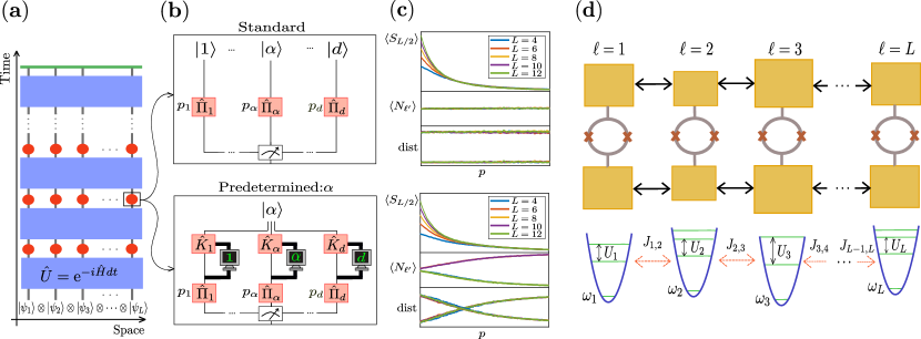
Figure 1: (a) Hybrid circuit of $L$ subsystems of dimension $d$ evolving under a unitary time evolution (blue rectangles) and probabilistic projective measurements (red circles) for an initial product state. The green line at the top corresponds to the steady state in which the observables are measured. (b) The standard measurements consists of a projective measurement $\hat{\Pi}_{n}=\ket{n}\bra{n}$ applied with a probability $p$ on each site $\ell$ whose outcome probabilities are given by Born’s rule $p_{n}=\braket{\psi}{\hat{\Pi}_{n}}{\psi}$, such that $\sum_{n=1}^{d}p_{n}=1$ defining $d$ different trajectories $\{\ket{1},\ket{2},...,\ket{d}\}$. The predetermined measurement consists of a standard measurement after which we access classically the result of the outcome (represented by the thick wire and the monitor), based on which we apply an outcome-dependent unitary operator $\hat{K}_{n}=\ket{n}\bra{\alpha}+\ket{\alpha}\bra{n}$ to the system forcing the subsystem to be in the state $\ket{\alpha}$ in all the trajectories. Note that here the measurement schemes are represented for a single site $\ell$, but the measurement is evaluated following a probability $p$ at every site and time step. (c) Numerical results for different observables averaged over circuit iterations at long times for $d=2$. For the standard measurement, the system undergoes a phase transition from a volume-law phase to an area-law phase with increasing measurement probability. Here the averaged results and distributions of simple observables do not provide any relevant critical information. For the predetermined measurement, we observe a similar phase transition but, in this case, the averaged results and, especially, its distribution provide useful statistical information about the phase transition location. (d) Scheme of an array of $L$ interacting transmons modeled as anharmonic oscillators with on-site energies $\omega_{\ell}$ and anharmonicities $U_{\ell}$, interacting capacitively with strengths given by $J_{\ell,\ell+1}$.

In Fig.1(a-b), we compare a standard measurement that produces one of $d$ possible results, with a predetermined measurement that projects the system to a predetermined state. Both are local projective measurements performed on a circuit composed of subsystems of arbitrary dimensions $d$. In the case of a standard measurement, $d$ different results can be produced after performing the measurement, thus defining $d$ different trajectories. A trajectory $n$ has a probability of occurrence $p_{n}$ given by Born’s rule. The state after the measurement is obtained by projecting the measured state by the operator $\hat{\Pi}_{n}=\ket{n}\bra{n}$. By contrast, the predetermined measurement consists of two events: first, a standard measurement is performed in the same way as in the previous case, and then a unitary operator $\hat{K}_{n}$, which depends on the result of the measurement $n$, is applied. This implies that we need to have short-term classical access to the result of the measurement to apply one or another unitary operator $\hat{K}_{n}$, thus forcing the system to be projected to a predetermined state and collapsing all the possible $d$ trajectories to a single one, without discarding any trajectory. After applying the unitary operation, information on the measurement outcome is unnecessary and does not need to be kept in a classical long-term memory. Therefore, the predetermined measurement can be understood as if we were to perform local quantum error correction in which we know the post-measurement state in advance. In this way, the probabilities associated with Born’s rule are eliminated being the measurement probability the only relevant parameter, and still eliminating the entanglement with the rest of the system.

Precisely, in this work, we propose that using predetermined measurements may inform us about the phase in which the system is located based on the statistical distribution of simple local observables without the need to carry out an explicit post-selection. In Fig. 1(c), we summarize the main result of the article. By measuring the boson number at one single site in the steady state, we can compare the distribution of the results with the theoretically expected distribution for area-law and volume-law phases. In the case of a standard measurement, the distributions are the same in the two phases, and therefore, the observable does not give any critical information. On the other hand, by introducing predetermined measurements, the boson number distributions are different in the area-law and volume-law phases. Therefore, we are able to indirectly find the expected approximate location of the phase transition as the crossing point of the fit of the observed distributions with the theoretical ones. Note that the distribution of the number of bosons at the steady states is obtained by merely collecting the outcomes, but it is not necessary to keep any other information. Importantly, the final results obtained for transmons modeling hard-core bosons are applicable to a wide range of scenarios, including arrays of subsystems with higher dimensions, disorder, and interactions. Both the analytical and numerical findings have a general nature, making them suitable for describing various systems.

The article is organized as follows: The attractive Bose-Hubbard model that describes the dynamics of interacting transmons is presented in Sec. II, along with creating a hybrid circuit consisting of unitary gates and non-unitary measurements. In Sec. III, we briefly describe the replica method approach to study the relevant statistical properties of the hybrid circuit encoded in the ground state of an effective non-Hermitian Hamiltonian, and we also introduce simple statistical arguments to adequately explain the dispersion of simple observables without using post-selection. In Section IV, we present the results for averaged observables in the area-law phase of hard-core bosons for both standard and predetermined measurements. Additionally, we suggest simple observables that can indirectly identify a phase transition in the entanglement entropy of individual trajectories when predetermined measurements are involved. In Sec. V we show numerical simulations to test the analytical predictions of the replica method for hard-core bosons. Finally, Sec. VI is dedicated to our conclusions and suggestions for future work.

II The model

To study a MIPT on an array of transmons undergoing projective measurements, we create a hybrid circuit consisting of unitary gates originating from the intrinsic dynamics of the transmons and non-unitary measurements introduced externally to monitor the system, see Fig. 1(a). Regarding the unitary elements, the dynamics of a one-dimensional array of $L$ interacting transmons [Fig. 1(d)] can be described by the disordered attractive Bose-Hubbard model [hacohen-gourgy15, roushan17] with Hamiltonian

$$\frac{\hat{H}}{\hbar}=\sum_{\ell=1}^{L}\left[\omega_{\ell}\hat{n}_{\ell}-\frac{U_{\ell}}{2}\hat{n}_{\ell}(\hat{n}_{\ell}-1)+J_{\ell}(\hat{a}_{\ell}^{\dagger}\hat{a}_{\ell+1}+\textrm{h.c.})\right],$$ (1)

where $\hat{a}_{\ell}$ and $\hat{a}^{\dagger}_{\ell}$ are the bosonic annihilation and creation operators at site $\ell$, which fulfill the commutation relations $[\hat{a}_{\ell},\hat{a}^{\dagger}_{\ell^{\prime}}]=\delta_{\ell,\ell^{\prime}}$, and $\hat{n}_{\ell}=\hat{a}^{\dagger}_{\ell}\hat{a}_{\ell}$ is the corresponding number operator. Within this description, $\omega_{\ell}$ accounts for the on-site energy and $U_{\ell}$ for the attractive interaction strength at site $\ell$, to which the bosonic excitations are subject. The term $J_{\ell}$ refers to the hopping rate of excitations between sites $\ell$ and $\ell+1$, and $J_{L}$ implicitly includes the boundary of the array, i.e. whether it has open or periodic boundary conditions. The Hamiltonian of Eq. (1) conserves the total number of excitations, since $[\hat{H},\hat{N}]=0$, where $\hat{N}=\sum_{\ell=1}^{L}\hat{n}_{\ell}$ is the total number operator. This implies that the dynamics occur in a single sector of a fixed number of excitations when initializing the system with a definite number of excitations.

For experimental purposes, it is convenient to take into account that the typical values of the parameters are around $\omega_{\ell}/2\pi\sim$5\text{\,}\mathrm{GHz}$$, $U_{\ell}/2\pi\sim~{}$200\text{\,}\mathrm{MHz}$$, and $J_{\ell}/2\pi\sim~{}$10\text{\,}\mathrm{MHz}$$ [koch2007, paik2011, arute2019], and range within the ratios $U_{\ell}/J_{\ell}\sim 2-30$ and $\omega_{\ell}/J_{\ell}\sim 50-1000$ [hacohen-gourgy15, roushan17]. Due to manufacturing defects, the exact parameter values differ between transmons and should be understood as being taken from a certain distribution. In most of the analysis, we will consider constant values $\omega_{\ell}\equiv\overline{\omega}$, $U_{\ell}\equiv\overline{U}$ and $J_{\ell}\equiv\overline{J}$, corresponding to the mean values of Gaussian distributions with variances $\sigma_{\omega}^{2}$, $\sigma_{U}^{2}$ and $\sigma_{J}^{2}$. Importantly, volume-law states can also be obtained even in the presence of a certain amount of disorder [Orell2019].

To create an analog circuit of the Bose-Hubbard Hamiltonian of Eq. (1), we use a Suzuki-Trotter decomposition to design a unitary layer corresponding to a time step $dt$ in terms of two-site gates [Pierkarska2018, Jaschke2018, Orell2019, Sieberer19, Barbiero2020, kargi21]. Briefly, we split the Hamiltonian of Eq. (1) into odd and even sites $\hat{H}=\sum_{\textnormal{odd }\ell}^{L}\hat{H}_{\ell}+\sum_{\textnormal{even }\ell}^{L}\hat{H}_{\ell}$, such that we can express the unitary time evolution operator as $e^{-i\hat{H}dt/\hbar}\approx\prod_{\text{even }\ell_{b}}^{L}e^{-i\hat{H}_{\ell_{b}}dt/\hbar}\prod_{\text{odd }\ell_{a}}^{L}e^{-i\hat{H}_{\ell_{a}}dt/\hbar}$ at first order in $dt$ (more details in App. A). After each layer of gates, we artificially introduce a probabilistic measurement layer in such a way that each time step, which is an effective layer of the hybrid circuit, can be expressed as

$$\ket{\widetilde{\psi}_{t+dt}}=\prod_{\ell_{c}}^{L}\hat{M}_{\ell_{c}}(p)\prod_{\text{even }\ell_{b}}^{L}e^{-i\hat{H}_{\ell_{b}}dt/\hbar}\prod_{\text{odd }\ell_{a}}^{L}e^{-i\hat{H}_{\ell_{a}}dt/\hbar}\ket{\widetilde{\psi}_{t}},$$ (2)

where $\hat{M}_{\ell}(p)$ represent the measurement operations performed with a certain probability $p$ at each site $\ell$. Furthermore, the state $\ket{\widetilde{\psi}_{t+dt}}$ needs to be renormalized due to the non-linearities that arise because of the non-unitary measurements. Note that we introduce the measurements ad hoc, assigning them a time scale $dt$ of the order of the trotterized gates, so we assume that the probability of performing a measurement at a particular site $\ell$ depends on the time scale $dt$ and a measurement rate $\Gamma$, such that $p=\Gamma dt$. For the numerical simulations, we define the layers simply by evolving the Hamiltonian (1) for a time $dt$ and then performing a measurement with a probability $p$, and finally renormalizing the state.

The type of measurement implemented is crucial, so we differentiate the two different cases based on the measurement operators $\hat{P}_{\ell}^{m}$ included in $M_{\ell}(p)$, where $m=0,1,...,d-1$ and $d$ is the dimension of each subsystem. First, we consider a standard measurement with operators $\hat{P}_{\ell}^{m}=\ket{m}\bra{m}$, whose outcome after performing a measurement range from $0$ to $d-1$ with an associate probability of occurrence given by the Born’s rule. Second, we introduce a predetermined measurement with operators $\hat{P}_{\ell}^{m}=\ket{\alpha_{\ell}}\bra{m}$, for a given set $[\alpha_{1},\alpha_{2},...,\alpha_{L}]$ that define the possible site-dependent outcomes after performing a measurement [note that $\hat{P}_{m}\equiv\hat{K}_{m}\hat{\Pi}_{m}$ in Fig. 1(b)]. This measurement can be understood as a correction in the following sense: first, a standard measurement is performed at site $\ell$ whose result depends on Born’s rule; second, we classically access this result, and, third, based on this, we perform a local operation on the site $\ell$ to project it onto state $\ket{\alpha_{\ell}}$. Importantly, these projectors do not break the permutation symmetry that is involved in the MIPT; it has been similarly considered in [Czischek2021, piroli2023]. In both cases, the operators fulfill the measurement condition $\sum_{m=0}^{d-1}(\hat{P}_{\ell}^{m})^{\dagger}(\hat{P}_{\ell}^{m})=\hat{I}$, although interestingly the standard measurement conserves the total number of bosons while the predetermined measurement does not.

III Statistical study

III.1 Replica method

After creating the hybrid circuit, which includes unitary gates with random parameters and interleaved probabilistic measurements that produce random or non-random outcomes based on the measurement type, we can analyze its long-term statistical behavior. However, this analysis becomes complex due to the numerous possibilities involved, both analytically and experimentally. For the analytical study of the statistical properties of the system, we will make use of the replica method, which has been used to describe simple random unitary circuits [zhou19, vasseur19, barbier21] where non-unitary measurements can be introduced [bao20], as well as additional symmetries [bao21], and whose statistical properties can be mapped to a classical mechanics model in which relevant statistical properties can be easily calculated, allowing us to study phase transitions in the entanglement entropy [jian21, jian21b].

For the implementation of the replica method to the Bose-Hubbard model with interspersed measurements (used differently in Ref. [Pierkarska2018]), we will focus on the work carried out by Bao et al. in Ref. [bao21], considering circuits that conserve the total number of bosons [oshima2023] instead of the $\mathbb{Z}_{2}$ symmetry-preserving circuits studied there. The symmetry of the conserved total number of bosons can be broken by the presence of predetermined measurements. Since we are interested in the ensemble of trajectories, we start by labeling the states at time $t$ with a sequence of measurement outcomes $m_{\bm{i}}$ and a set of gate parameters $\theta_{\mathbb{i}}$ as:

$$\hat{\tilde{\rho}}_{m_{\mathbb{i}},\theta_{\mathbb{i}}}(t)=\left(\hat{P}_{m_{t}}\hat{U}_{\theta_{t}}\cdots\hat{P}_{m_{1}}\hat{U}_{\theta_{1}}\right)\hat{\rho}_{0}\left(\hat{U}_{\theta_{1}}^{\dagger}\hat{P}_{m_{1}}^{\dagger}\cdots\hat{U}_{\theta_{t}}^{\dagger}\hat{P}_{m_{t}}^{\dagger}\right),$$ (3)

where $\hat{\rho}_{0}$ is the initial state, $\hat{U}_{\theta_{\mathbb{i}}}$ are the set of unitary evolution gates, $\hat{P}_{m_{\mathbb{i}}}$ are the projection operators associated with measurement outcomes $m_{\mathbb{i}}$, and $\mathbb{i}$ refers to all the positions in the circuit space-time. For studying the steady-state properties of the ensemble of states $\hat{\tilde{\rho}}_{m_{\mathbb{i}},\theta_{\mathbb{i}}}(t)$, and its associated probabilities, we consider the dynamics of $n$ copies—the replicas—of the density matrices $\ket{\ket{\tilde{\rho}_{m_{\mathbb{i}},\theta_{\mathbb{i}}}^{(n)}}}\equiv\hat{\tilde{\rho}}_{m_{\mathbb{i}},\theta_{\mathbb{i}}}^{\otimes n}$ interpreted as state vectors in the replicated Hilbert space $\mathcal{H}^{(n)}=(\mathcal{H}\otimes\mathcal{H}^{*})^{\otimes n}$, on which unitary $\check{\mathcal{U}}_{\theta_{i}}^{(n)}\equiv(\hat{U}_{\theta_{i}}\otimes\hat{U}_{\theta_{i}}^{*})^{\otimes n}$, and measurement projection operators $\check{\mathcal{M}}_{m_{i}}^{(n)}\equiv(\hat{P}_{m_{i}}\otimes\hat{P}_{m_{i}}^{\dagger})^{\otimes n}$ act, as well as general operators $\check{\mathcal{O}}^{(n)}\equiv(\hat{O}\otimes\hat{I})^{\otimes n}$ that are going to be used for computing observables.

Taking into account the non-normalized averaged state of the ensemble $\ket{\ket{\tilde{\rho}^{(n)}(t)}}=\sum_{m_{\mathbb{i}},\theta_{\mathbb{i}}}\ket{\ket{\tilde{\rho}_{m_{\mathbb{i}},\theta_{\mathbb{i}}}^{(n)}(t)}}=e^{-t\check{\mathcal{H}}_{\textnormal{eff}}}\ket{\ket{\rho_{0}^{(n)}}}$, we can exactly map the dynamics to an imaginary time evolution generated by an effective quantum Hamiltonian $\check{\mathcal{H}}_{\textnormal{eff}}$, such that the properties of the averaged state of the ensemble at long times are encoded in its ground state. Note that from now on we will consider $\hbar=1$ to simplify the notation. Using this formalism, we can compute the trajectory-averaged $k$-moment of an observable $\hat{O}$, which is given by

$$\overline{\left\langle O_{k}\right\rangle}= \lim_{n\to 1}\frac{\braket{\braket{\mathcal{I}^{(n)}}{\check{\mathcal{O}}_{k}^{(n)}}{\tilde{\rho}^{(n)}}}{missing}{missing}}{\braket{\braket{\mathcal{I}^{(n)}}{\tilde{\rho}^{(n)}}}{missing}}=\lim_{n\to 1}O_{k}^{(n)},$$ (4)

where $\overline{\cdot}$ refers to the average over gate parameters and $\left\langle\cdot\right\rangle$ to the average over measurements outcomes and the inner product is defined by $\braket{\braket{\mu}{\sigma}}{\equiv}\operatorname{tr}\left(\hat{\mu}^{\dagger}\hat{\sigma}\right)$, for arbitrary states $\hat{\mu}$ and $\hat{\sigma}$ and a reference state $\ket{\ket{\mathcal{I}^{(n)}}}$ in the replicated Hilbert space. Therefore, the quantities we are going to study for addressing phase transitions are the objects $O_{k}^{(n)}$ in Eq. (4), which corresponds to the exact trajectory-averaged quantum mechanical observables only in the replica limit $n\to 1$. It has been shown, at least for the von Neumann entropy that, although not being the same quantity, both share critical properties in the MIPT [bao20]. More details on this particular implementation of the formalism can be found in App. B and in Ref. [bao21].

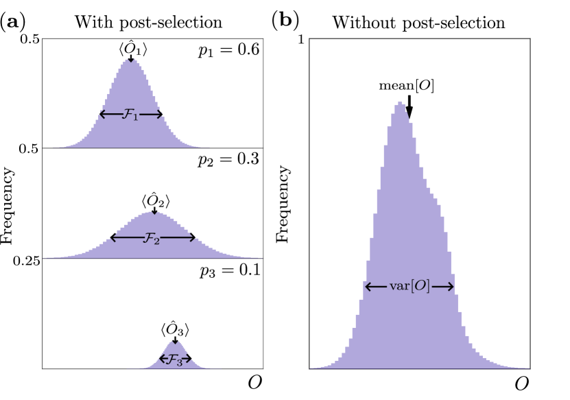
Figure 2: A toy model schematic highlighting experimental differences in computing the mean and variance of an arbitrary observable $\hat{O}$ with and without post-selection. For the sake of simplicity, in this example, the circuit produces only three different trajectories with associated probabilities $\{p_{1},p_{2},p_{3}\}$, and each count in the bins corresponds to final measurements made at long times for a total of $10^{7}$ iterations of the circuit, represented as the relative frequency. (a) Post-selected histogram of the distribution of measurement outcomes: We separate each of the iterations of the circuit by grouping them into the three different subgroups of trajectories, such that the mean values of the distribution of the observable correspond to the expectation values $\{\braket{\hat{O}_{1}},\braket{\hat{O}_{2}},\braket{\hat{O}_{3}}\}$ and the variances to the fluctuations $\{\mathcal{F}_{1},\mathcal{F}_{2},\mathcal{F}_{3}\}$ of the operator $\hat{O}$ for each type of trajectory, which they are pure states. (b) Histogram of the measurement outcomes without post-selection: We mix all the iterations of the circuit without taking into account to which trajectory corresponds, and compute the mean value $\textnormal{mean}[O]$ and variance $\textnormal{var}[O]\equiv\Delta O$ of the distribution of the observable $\hat{O}$ among all iterations. Since the mean values involve the first moment $k=1$, it is fulfilled that $\textnormal{mean}[O]\equiv\overline{\braket{O_{1}}}=p_{1}\braket{\hat{O}_{1}}+p_{2}\braket{\hat{O}_{2}}+p_{3}\braket{\hat{O}_{3}}$. However, the fluctuations of the operator involve the second moments $k=2$, so $\overline{\braket{\mathcal{F}}}=p_{1}\mathcal{F}_{1}+p_{2}\mathcal{F}_{2}+p_{3}\mathcal{F}_{3}$ and $\Delta O$ will give similar results only under certain conditions, see Eqs. (8) and (12).

III.2 Direct average of circuit realizations

Next, we will expose the role of the moment $k$ of Eq. (4) in the post-selection of trajectories to calculate trajectory-averaged quantities. For that, it is useful to express the trajectory-averaged quantities in terms of the measurement probability $p$ and probability distributions of the gate parameters $p_{\theta_{\mathbb{i}}}$ and the outcomes of the interleaved measurements $p_{m_{\mathbb{b}}}(\theta)$, such that

$$\overline{\langle O_{k}\rangle}=\sum_{b=0}^{M}p^{b}(1-p)^{M-b}\langle O_{k}^{b}\rangle_{\textnormal{m},\theta},$$ (5)

where the average expectation value is

$$\langle O_{k}^{b}\rangle_{\begin{subarray}{c}\textnormal{m},\theta\end{subarray}}=\int d\theta_{\mathbb{i}}\sum_{\mathbb{b}}^{\binom{M}{b}}\sum_{m_{\mathbb{b}}}^{d^{b}}p_{m_{\mathbb{b}},\theta_{\mathbb{i}}}\left[\operatorname{tr}\left(\hat{O}\hat{\rho}_{m_{\mathbb{b}},\theta_{\mathbb{i}}}\right)\right]^{k},$$ (6)

where and $\hat{O}$ can be any operator and $p_{m_{\mathbb{b}},\theta_{\mathbb{i}}}\equiv p_{\theta_{\mathbb{i}}}p_{m_{\mathbb{b}}}(\theta)$, $\binom{M}{b}=\frac{M!}{b!(M-b)!}$, $\mathbb{b}$ is an array with all the possible $\binom{M}{b}$ combinations of arranging $b$ measurements in the total $M$ positions of space-time. In other words, $M$ is the maximum number of measurements that is performed when $p=1$ and $\mathbb{b}=\mathbb{i}$; while no measurements are performed when $p=0$ and $\mathbb{b}=\emptyset\to p_{m_{\mathbb{b}},\theta_{\mathbb{i}}}=p_{\theta_{\mathbb{i}}}$. The probability distributions are normalized such that $\sum_{b=0}^{M}p^{b}(1-p)^{M-b}{\binom{M}{b}}=1$, $\sum_{m}^{d^{b}}p_{m_{\mathbb{b}}}(\theta)=1$ and $\int d\theta_{\mathbb{i}}p_{\theta_{\mathbb{i}}}=1$. We have considered that $p_{m_{\mathbb{i}}}(\theta_{\mathbb{i}})\to p_{m_{\mathbb{b}}}(\theta_{\mathbb{i}})$, because for the probability distribution we need to take into account those positions $\mathbb{b}$ where measurements have been performed and not all the possible positions $\mathbb{i}$ where a measurement could have been performed.

We can interpret that the trajectory-averaged first moment $k=1$ quantities, such as the number of bosons $\overline{\braket{N_{1}}}$ or the dispersion of the number of bosons over different circuit iterations $\Delta N$, can be obtained in a realistic experimental device by averaging all the results obtained from different experiments, i.e. iterations, without taking into account the final states. By contrast, the trajectory-averaged second moment $k=2$ quantities, such as the second Rényi entanglement entropy (related to the von Neumann entropy $\overline{\braket{S}}$ in the replica limit) and the fluctuation of the number operator $\overline{\braket{\mathcal{F}}}$ [agrawal2022, oshima2023], require to repeat the experiment for each final state independently, post-selecting the different trajectories from the different iterations of the circuit (Fig. 2). Throughout the paper, we exclusively compute observables from individual trajectories without calculating the averaged density matrix. For simple observables like the number of bosons, the computed value matches that obtained from the averaged density matrix.

The role of $k$ can be seen by simplifying Eqs. (5) and (6) to a generic expression $\overline{f}=\sum_{x}p_{1}(x)\sum_{y}[p_{2}(x,y)f(y)]^{k}$ where $p_{1}(x)$ is the probability of each trajectory and $p_{2}(x,y)$ is the probability of obtaining the different outcomes $f(y)$. This can be further simplified as $\overline{f}=\sum_{z}p(z)f(z)$ if $k=1$ and thus obtained from a general distribution, i.e. collecting results from different experiments without taking into account the trajectories. Here $p(z)$ is the probability of obtaining an outcome $f(z)$. The simplification does not hold for a general case if $k\geq 2$. Notice the subtle difference between averaging over trajectories analytically and averaging over iterations of the circuit numerically/experimentally, see Fig. 2 and App. LABEL:appsec:numerical_simulation.

We can go further and use the simple way of describing trajectory-averaged quantities in Eq. (5), to study quantities related to the variance of observables in the high measurement regime. In what follows, we consider the first $k=1$ and second $k=2$ moments of observables related to the boson number without any disorder in the parameters, such that Eq. (5) becomes

$$\langle N_{k}\rangle=\sum_{b=0}^{M}p^{b}(1-p)^{M-b}\sum_{\mathbb{b}}^{\binom{M}{b}}\sum_{m}^{d^{b}}p_{m_{\mathbb{b}}}[\operatorname{tr}(\hat{N}\hat{\rho}_{m_{\mathbb{b}}})]^{k},$$ (7)

where the usual number of bosons is given for $k=1$. We are particularly interested in the trajectory-averaged fluctuations of $\hat{N}$ for each trajectory

$$\langle\mathcal{F}\rangle= \sum_{b=0}^{M}p^{b}(1-p)^{M-b}$$ (8)

$$\times\sum_{\mathbb{b}}^{\binom{M}{b}}\sum_{m}^{d^{b}}p_{m_{\mathbb{b}}}\left\{\operatorname{tr}\left(\hat{N}^{2}\hat{\rho}_{m_{\mathbb{b}}}\right)-\left[\operatorname{tr}(\hat{N}\hat{\rho}_{m_{\mathbb{b}}})\right]^{2}\right\},$$

for which we calculate the variance of $\hat{N}$ for the final state of each trajectory, and then we average over all possible trajectories. We are also going to calculate the dispersion in the number of bosons with the average given by Eq. (7)

$$\Delta N\equiv \langle(N^{2})_{1}\rangle-\langle N_{1}\rangle^{2}.$$ (9)

To simplify notation, we now omit the sub-index $k=1$ when referring to the number of bosons.

The quantities of Eqs. (7)-(9) are typically difficult to evaluate, but we can derive useful expressions by making certain assumptions. The following results are obtained for a large measurement probability close to a perfectly measured system, as described in App. LABEL:appsec:circuit_average. Trajectory-averaged fluctuation of the number operator in the half of the chain, considering a predetermined measurement with spatial pattern $\overline{\alpha}={\alpha_{1},\alpha_{2},...,\alpha_{L}}$ and up to second order in $x\equiv(1-p)$, is given by

$$\braket{\mathcal{F}_{\frac{L}{2}}}\approx x^{2}\left[(\alpha_{\frac{L}{2}}+1)\alpha_{\frac{L}{2}+1}+\alpha_{\frac{L}{2}}(\alpha_{\frac{L}{2}+1}+1)\right]\left(\frac{J}{\Gamma}\right)^{2}.$$ (10)

We can also obtain the dispersion of the number of bosons in the half of the chain, which is not a trajectory-averaged quantity but the variance of the number of bosons of all circuit iterations. The calculations are a bit cumbersome, but it is enough to consider up to the first order in $x\equiv(1-p)$ to observe that there is a dependency on the size of the system,

$$\Delta N_{\frac{L}{2}}\approx xg(\overline{\alpha},L)\left(\frac{J}{\Gamma}\right)^{2},$$ (11)

where the exact expression of the function $g(\overline{\alpha},L)$ can be found in Eq. (LABEL:DN_nonconserving_app). However, this dependency is due to the non-conservation of the total number of bosons of the predetermined measurement. Selecting only the iterations where the total number of bosons coincides with $N_{\overline{\alpha}}=\sum_{\ell=1}^{L}\alpha_{\ell}=N_{T}$, we recover the same behavior as for the fluctuation up to the second order,

$$\Delta N_{\frac{L}{2}}^{N_{\overline{\alpha}}}\approx x^{2}\left[(\alpha_{\frac{L}{2}}+1)\alpha_{\frac{L}{2}+1}+\alpha_{\frac{L}{2}}(\alpha_{\frac{L}{2}+1}+1)\right]\left(\frac{J}{\Gamma}\right)^{2}.$$ (12)

Note that this last result does not imply post-selection as such. It only requires measuring the number of bosons at each site at the end of time evolution as a measure of the observable of interest, keeping the results with a total number $N_{\overline{\alpha}}$ and calculating the variance of the number distribution of bosons for the middle of the chain avoiding post-selection in a similar way as in [ippoliti21c]. Note that $\overline{\braket{\mathcal{F}}}$ and $\Delta N$ are essentially different quantities and have the same behavior for the predetermined measurement, but not for the standard measurement case. However, at least deep in the area-law phase, it is expected that $\Delta N$ overestimates the volume-law phase. It is important to keep in mind that $\overline{\braket{\mathcal{F}}}$ behaves like $\overline{\braket{S}}$, so the interest in measuring quantities such as $\Delta N^{N_{\overline{\alpha}}}$, which is equal to $\overline{\braket{\mathcal{F}}}$ in a certain regime, is to have observables that do not require post-selection to indirectly measure the entanglement.

III.3 Boson dynamics in an enlarged space

For the sake of simplicity, from now on we consider $n=2$ replicas, which is the lowest number of replicas needed to capture the relevant MIPT properties [bao20, bao21]. The transfer matrix between the state of the system at $t+dt$ and $t$ is then obtained by averaging the evolution over the distribution of unitary gates and the probabilities $p=\Gamma dt$ of applying measurement operators At first order in $dt$, we have that $\prod_{\ell^{\prime}}^{L}\braket{\check{\mathcal{M}}_{\ell^{\prime}}}\prod_{\ell}^{L}\overline{\check{\mathcal{U}}_{\ell}}\simeq e^{-dt\check{\mathcal{H}}_{\textnormal{eff}}}$, where the effective Hamiltonian is given by

$$\check{\mathcal{H}}_{\textnormal{eff}}=\sum_{\ell}^{L} \left\{\Gamma_{\ell}\left(\check{\mathcal{I}}-\sum_{m_{\ell}}^{d}\check{\mathcal{P}}_{m_{\ell}}\right)\right.$$ (13)

$$\left.+i\left[\overline{\omega}\check{\mathcal{n}}_{\ell}+\overline{J}\left(\check{\mathcal{a}}_{\ell}^{\dagger}\check{\mathcal{a}}_{\ell+1}+\check{\mathcal{a}}_{\ell}\check{\mathcal{a}}_{\ell+1}^{\dagger}\right)-\frac{\overline{U}}{2}\check{\mathcal{u}}_{\ell}\right]\right\},$$

where each $\check{\mathcal{P}}_{m_{\ell}}$ derives from a measurement operator and acts on the two replicas, $\check{\mathcal{n}}_{\ell}$, $\check{\mathcal{a}}_{\ell}$, $\check{\mathcal{a}}_{\ell}^{\dagger}$ and $\check{\mathcal{u}}_{\ell}$ derive from the unitary gates and each of them are composed of operators acting on one of the replicas, and finally $\check{\mathcal{I}}$ is the identity operator. The exact expressions can be found in App. B, see Eqs. (44)-(47). By means of the effective Hamiltonian of Eq. (13), we will compute different trajectory-averaged observables, related to the first moment $k=1$ not requiring post-selection and second moment $k=2$ requiring post-selection: $S^{(2)}$ is the $2$-conditional Renyi entropy that results in the properly trajectory-averaged von Neumann entropy in the replica limit in Eq. (LABEL:observable_entropy), and, similarly, the other trajectory-averaged quantities result, in the replica limit, in the number of bosons $N^{(2)}$ in Eq. (LABEL:observable_number) and the fluctuation of the number operator $\mathcal{F}^{(2)}$ in Eq. (LABEL:observable_fluctuation).

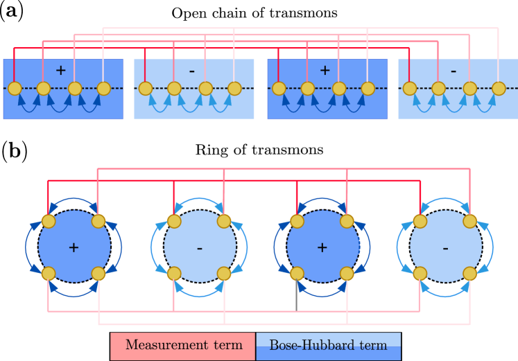
Figure 3: Scheme of the enlarged space where the effective Hamiltonian $\hat{H}_{\textnormal{eff}}$ is defined for a hybrid circuit of $L=4$ transmons (yellow circles) arranged (a) linearly or (b) in a ring configuration. Each rectangle represents the blocks of the replicas (dark blue for the kets and light blue for the bras) and the sign is given by the Eq. (17). All the terms belonging to the operator with origin in the measurements [red lines, Eq. (15)] act on all the blocks of all replicas, while the terms belonging to the operator with origin in the unitary evolution of the Bose-Hubbard Hamiltonian [blue areas and arrows, Eq. (16)] act on each block independently.

The ground state of the effective Hamiltonian of Eq. (13) encapsulates the statistical information of the ensemble of trajectories of the original hybrid circuit at long times, which allows us to compute relevant trajectory-averaged quantities related to the entanglement entropy and the number of bosons. Unlike previous works [bao21], in this case, the effective Hamiltonian given by $\check{\mathcal{H}}_{\textnormal{eff}}=\check{\mathcal{H}}_{\mathcal{M}}+i\check{\mathcal{H}}_{\mathcal{U}}$ is non-Hermitian. This kind of dynamics has been used before for describing other continuously measured systems [thiel20, dubey21, gopalakrishnan21]. Note that the term $\check{\mathcal{H}}_{\mathcal{U}}$ is Hermitian since it has its origin in the replicated Bose-Hubbard Hamiltonian, while the term $\check{\mathcal{H}}_{\mathcal{M}}$ has its origin in the measurements and its hermicity will depend on the type of measurements implemented in the circuit: the standard measurement yields a Hermitian operator, while a predetermined measurement yields a non-Hermitian operator since it is real and non-symmetric.

To study the ground state of the Hamiltonian in Eq. (13) it is useful to interpret it as an effective Bose-Hubbard Hamiltonian in an enlarged space so that the bosons move in an enlarged space and have additional interacting terms arising from measurements. This implies that the $d^{4L}$-dimensional effective Hamiltonian $\check{\mathcal{H}}_{\textnormal{eff}}=\check{\mathcal{H}}_{\mathcal{M}}+i\check{\mathcal{H}}_{\mathcal{U}}$ constructed by the tensor product of four copies of operators describing dynamics in a $L$-sites real space becomes a $d^{4L}$-dimensional effective Hamiltonian $\hat{H}_{\textnormal{eff}}=\hat{H}^{M}+i\hat{H}^{\rm BH}$ formed by operators describing the dynamics in a $4L$-sites enlarged space. Therefore, the original circuit consisting of $L$ transmons defines four different blocks in this enlarged space of $4L$ sites: $[1,L]$, $[L+1,2L]$, $[2L+1,3L]$ and $[3L+1,4L]$ (Fig. 3). In this way, the term $\hat{H}^{M}$ represents an interaction between blocks at the sites $l,l+L,l+2L,l+3L$ where $l$ corresponds to the site $\ell$ of the circuit where the measurement is performed, while $\hat{H}^{\rm BH}$ is simply a Bose-Hubbard Hamiltonian of $4L$ sites, whose parameters, i.e. $\overline{J}$, $\overline{\omega}$ and $\overline{U}$, have different signs between contiguous blocks. Note that the local terms of the on-site energies $\overline{\omega}$ and interactions $\overline{U}$ cover the full $4L$ space, while the hopping terms $\overline{J}$ are zero between the blocks. Therefore, we can reinterpret the terms of the effective Hamiltonian (13) in such a way that

$$\hat{H}_{\textnormal{eff}}=\hat{H}^{M}+i\hat{H}^{\rm BH},$$ (14)

where the measurement and Bose-Hubbard terms are

$$\hat{H}^{\rm M} =\Gamma\sum_{l=1}^{L}\left(\hat{I}-\sum_{m=0}^{d-1}\hat{P}_{l}^{m}\hat{P}_{l+L}^{m}\hat{P}_{l+2L}^{m}\hat{P}_{l+3L}^{m}\right),$$ (15)

$$\hat{H}^{\rm BH} =\sum_{l=1}^{4L}W(l)\left[\overline{\omega}\hat{n}_{l}+\overline{J}\left(\hat{a}_{l}^{\dagger}\hat{a}_{l+1}+h.c.\right)-\frac{\overline{U}}{2}\hat{n}_{l}(\hat{n}_{l}-\hat{I})\right],$$ (16)

with the sign function

$$W(l)=\begin{cases}+1,l\in\left[1,L\right]\cup\left[2L+1,3L\right],\\ -1,l\in\left[L+1,2L\right]\cup\left[3L+1,4L\right].\end{cases}$$ (17)

Note that Eqs. (14)-(17), apply to both standard and predetermined measurements, the only difference lies in the specific projector $\hat{P}_{l}^{m}$ required for each case. For exact details about obtaining the vectorized states from operators and the averaged observables, see App. LABEL:appsec:replica_method_effective_hamiltonian_enlarged.

Since the effective Hamiltonian describes the statistical properties of the circuit trajectories, some of its features are expected to contain information about the phase transition. MIPT is directly related to a spontaneous symmetry breaking, which arises because the relevant quantities, such as entanglement entropy and fluctuations of observables, for the phase transition, can be observed only in the nonlinear moments of the density matrix, whose time evolution can be expressed by the evolution of $n\geq 2$ replicas [bao21]. In this way, the dynamic has a permutation symmetry between the $n$ replicas, that is, both between kets and between bras, which is preserved in the area-law phase and broken in the volume-law phase.

Thus, we can study the nature of the ground states of $\hat{H}_{\textnormal{eff}}$ to understand the spontaneous symmetry breaking in limiting cases of the measurement rate $\Gamma$ [altland22]. Deep in the area-law phase, when $\Gamma\to\infty$, the term $\hat{H}^{M}$ predominates, and for the case of predetermined measurements, there is a non-degenerate ground state that is independent of the number of replicas, for which preserves the permutation symmetry. It can be seen in Fig. 3 that adding replicas does not affect the degeneracy of the ground state. Note that in the case of using a standard measurement, there are $d^{L}$ degenerated ground states corresponding to the possible outcomes of the measurements that are also independent of the number of replicas. Deep in the volume-law phase, when $\Gamma\to 0$, the term $\hat{H}^{\rm BH}$ predominates the effective Hamiltonian, in which, as we see in Fig. 3, the number of terms increases by adding replicas. However, in the effective Hamiltonian, $\hat{H}^{\rm BH}$ is purely imaginary at order $dt$, and therefore does not have a well-defined ground state (all eigenstates have a zero real part and the degeneracy trivially increases by increasing the number of replicas). But at higher orders of $dt$, $\hat{H}^{\rm BH}$ does have real components [bao21], whose terms also depend on the number of replicas, thus increasing the degeneracy of the ground states with the number of replicas, and breaking the permutation symmetry. Note that we cannot directly use the second-order term in the expression for the evolution operator in the replica space, Eq. (41), since it would be necessary to have previously performed a second-order Suzuki-Trotter decomposition, making the analytical expression considerably cumbersome. These are general arguments, to prove the existence of a MIPT, each case must be addressed individually and verified through numerical finite-size scaling analysis.

IV Trajectory-averaged observables

In this section, we derive analytical expressions for the trajectory-averaged observables as functions of the measurement rate $\Gamma$. We use the replica-method formalism and appropriately apply the non-Hermitian perturbation theory for each measurement type. We provide specific results for hard-core bosons in the area-law phase, but the main results can be extended to higher dimensions at low measurement rates.

IV.1 Perturbation theory for non-Hermitian Hamiltonians

The non-hermicity of the Hamiltonian of Eq. (14) hinders the use of standard quantum mechanical techniques to determine its ground state, mainly due to the non-orthogonality of eigenvectors. Thus, we will follow the bi-orthogonal quantum mechanical formalism [sterheim1972, Brody_2013], in which we obtain the eigenstates and eigenenergies for the operator $\hat{H}_{\textnormal{eff}}\ket{\phi_{m}}=E_{m}\ket{\phi_{m}}$ and its Hermitian conjugate $\hat{H}_{\textnormal{eff}}^{\dagger}\ket{\tilde{\phi}_{m}}=\tilde{E}_{m}\ket{\tilde{\phi}_{m}}$. In this way, although if $[\hat{H}^{M},\hat{H}^{\rm BH}]\neq 0$ the orthogonality of eigenstates $\braket{\phi_{m}}{\phi_{n}}=0$ for $E_{m}\neq E_{n}$ is no longer met, we have that $\tilde{E}_{n}=E_{n}^{*}$ is fulfilled, and $\{\tilde{\phi}_{m},\phi_{m}\}$ forms a bi-orthogonal set such that $\braket{\tilde{\phi}_{m}}{\phi_{n}}=\delta_{m,n}$ and $\hat{I}=\sum_{m}\ket{\phi_{m}}\bra{\tilde{\phi}_{m}}$. The ground state will be defined as the eigenstate with the lowest real part of the eigenenergy $\mathfrak{Re}(\braket{\tilde{\phi}}{\hat{H}_{\textnormal{eff}}}{\phi})$.

Since obtaining the exact analytical expression for the ground state of $\hat{H}_{\textnormal{eff}}$ is rather complicated, we will make use of the perturbation theory. We can define two regimes as a function of the measurement rate $\Gamma$: volume-law phase, where $\Gamma/\overline{J},\overline{\omega},\overline{U}\ll 1$ and $\hat{H}^{\rm M}$ acts as a perturbation; and area-law phase, where $\Gamma/\overline{J},\overline{\omega},\overline{U}\gg 1$ and $\hat{H}^{\rm BH}$ acts as an imaginary perturbation. In this work, we will focus on the area-law phase. Briefly, we expand the eigenenergies and eigenstates in terms of the parameter $\lambda\equiv\overline{J}/\Gamma\ll 1$ and solve the Schrödinger equation for $\hat{H}_{\textnormal{eff}}$ and $\hat{H}_{\textnormal{eff}}^{\dagger}$ (see Eqs. (LABEL:H_expanded_lambda)-(LABEL:Hdagger_expanded_lambda) in App. LABEL:appsec:non-Hermitian). The normalized correction for the non-degenerate state $\ket{\phi_{\alpha}}$ and energies up to second order in $\lambda$ are

$$\ket{\phi_{\alpha}}_{N}= \left[1+\frac{\lambda^{2}}{2}\sum_{n\neq\alpha}\frac{V_{n\tilde{\alpha}}^{*}V_{\tilde{n}\alpha}}{(\tilde{E}_{\alpha}^{(0)*}-\tilde{E}_{n}^{(0)*})(E_{\alpha}^{(0)}-E_{n}^{(0)})}\right]\ket{\phi_{\alpha}^{(0)}}$$

$$\quad+i\lambda\sum_{n\neq\alpha}\frac{V_{\tilde{n}\alpha}}{(E_{\alpha}^{(0)}-E_{n}^{(0)})}\ket{\phi_{n}^{(0)}}$$

$$\quad-\lambda^{2}\sum_{n,m\neq\alpha}\frac{V_{\tilde{n}m}V_{\tilde{m}\alpha}}{(E_{\alpha}^{(0)}-E_{n}^{(0)})(E_{\alpha}^{(0)}-E_{m}^{(0)})}\ket{\phi_{n}^{(0)}}$$

$$\quad+\lambda^{2}\sum_{n\neq\alpha}\frac{V_{\tilde{\alpha}\alpha}V_{\tilde{n}\alpha}}{(E_{\alpha}^{(0)}-E_{n}^{(0)})^{2}}\ket{\phi_{n}^{(0)}},$$ (18)

$$E_{\alpha}= E_{\alpha}^{(0)}+i\lambda V_{\tilde{\alpha}\alpha}-\lambda^{2}\sum_{n\neq\alpha}\frac{V_{\tilde{\alpha}n}V_{\tilde{n}\alpha}}{(E_{\alpha}^{(0)}-E_{n}^{(0)})}$$ (19)

where the matrix elements are $V_{\tilde{a}b}=\braket{\tilde{\phi}_{a}^{(0)}}{\hat{H}^{\rm BH}}{\phi_{b}^{(0)}}$ and $V_{a\tilde{b}}=\braket{\phi_{a}^{(0)}}{\hat{H}^{\rm BH}}{\tilde{\phi}_{b}^{(0)}}$. It can be shown that up to the second order in $\lambda$, the on-site energy $\sum_{l}^{4L}W(l)\hat{n}_{l}$ and interaction $\sum_{l}^{4L}W(l)\hat{n}_{l}(\hat{n}_{l}-\hat{I})$ terms do not play any role in obtaining the different quantities of Eqs. (LABEL:observable_entropy)-(LABEL:observable_number) because they vanish by their symmetry. We obtain the same result with the different approach considered in App. (LABEL:appsec:circuit_average), see Eq. (LABEL:observables_circuit_dt4_app). This implies that in the high measurement regime $\overline{J}/\Gamma\ll 1$ i.e. deep in the area-law phase, we just need to focus on the hopping terms $\sum_{l}^{4L}W(l)\overline{J}(\hat{a}_{l}^{\dagger}\hat{a}_{l+1}+h.c.)$.

IV.1.1 Predetermined measurements in transmons

To study the predetermined measurement, we need to establish a predetermined spatial profile for the local number of bosons $\{\alpha_{1},\alpha_{2},\dots,\alpha_{L}\}$ where $\alpha_{\ell}=0,1,\dots,d-1$, which will be forced by the measurement at each site in the original circuit $\ell\in[1,L]$. Although we focus on non-absorbing states, they can be achieved by setting all $\alpha_{\ell}$ either to zero or to $d-1$. The associated projectors will be given by $\hat{P}_{\ell}^{m}=\ket{\alpha_{\ell}}\bra{m}$, where $\sum_{m=0}^{d-1}(\hat{P}_{\ell}^{m})^{\dagger}(\hat{P}_{\ell}^{m})=\hat{I}$. Since $\hat{H}^{M}$ is non-Hermitian because it is a real non-symmetric operator that does not conserve the total number of bosons, we cannot use the boson number basis of $\hat{N}=\sum_{l}^{4L}\hat{n}_{l}$ as the unperturbed basis, and we need to obtain the full bi-orthogonal basis explicitly. We can start by considering the bi-orthogonal basis for the unperturbed effective Hamiltonian of one transmon of dimension $d$, which is given by

$$\ket{\phi}=\begin{cases}\ket{\overline{\alpha_{\ell}}},&E=0,\quad\#1\\ \ket{\overline{a}}-\ket{\overline{\alpha_{\ell}}},&E=1,\quad\#d-1\\ \ket{ijkl},&E=1,\quad\#d^{4}-d\end{cases}$$ (20)

$$\ket{\tilde{\phi}}=\begin{cases}\sum_{x=0}^{d-1}\ket{\overline{x}},&\tilde{E}=0,\quad\#1\\ \ket{\overline{b}},&\tilde{E}=1,\quad\#d-1\\ \ket{mnpq},&\tilde{E}=1,\quad\#d^{4}-d\end{cases}$$ (21)

where $\alpha_{\ell},a,b,i,j,k,l,m,n,p,q=0,1,...,d-1$ and satisfy the following conditions: $a\neq\alpha_{\ell}$, $b\neq\alpha_{\ell}$, no $i=j=k=l$, and no $m=n=p=q$. Note that we adopt the notation $\ket{\overline{n}}\equiv\ket{nnnn}$. The basis for the unperturbed effective Hamiltonian has a dimension $D=d^{4}$, fulfills the bi-orthonormality condition $\braket{\tilde{\phi}_{i}}{\phi_{j}}=\delta_{ij}$, and has a non-degenerate ground state. For obtaining the eigenstates for an arbitrary number of transmons $L$, we consider all possible combinations of Eqs. (20)-(21), such that

$$\ket{\Phi_{i_{1},i_{2},...,i_{L}}^{pre}}=\ket{\phi_{i_{i}}}\ket{\phi_{i_{2}}}\cdots\ket{\phi_{i_{L}}},$$ (22)

$$\ket{\tilde{\Phi}_{i_{1},i_{2},...,i_{L}}^{pre}}=\ket{\tilde{\phi}_{i_{i}}}\ket{\tilde{\phi}_{i_{2}}}\cdots\ket{\tilde{\phi}_{i_{L}}},$$ (23)

where $i_{1},i_{2},..,i_{L}$ are indices that run over all $d^{4}$ possibilities in the Eqs. (20)-(21), $\braket{\tilde{\Phi}_{i_{1},i_{2},...,i_{L}}}{\Phi_{j_{1},j_{2},...,j_{L}}}=\delta_{i_{1},j_{1}}\delta_{i_{2},j_{2}}\cdots\delta_{i_{L},j_{L}}$, and the total dimension is $D=d^{4L}$. Note that the energy is given by $0\leq E_{i_{1},i_{2},...,i_{L}}=\sum_{\ell=1}^{L}(1-\delta_{i_{\ell},1})\leq L$, such that the ground states have an energy $E_{1,1,...,1}=\tilde{E}_{1,1,...,1}=0$, and are given by

$$\ket{\Phi_{1,1,...,1}^{pre}}=\ket{\overline{\alpha_{1}}}\ket{\overline{\alpha_{2}}}\cdots\ket{\overline{\alpha_{L}}},$$ (24)

$$\ket{\tilde{\Phi}_{1,1,...,1}^{pre}}=\sum_{x_{1},x_{2},...x_{L}=0}^{d-1}\ket{\overline{x_{1}}}\ket{\overline{x_{2}}}\cdots\ket{\overline{x_{L}}},$$ (25)

where ${\alpha_{1},\alpha_{2},...,\alpha_{L}}$ are the boson number subspace projected at each site. For obtaining the bi-orthogonal basis, we have made use of a different notation which eases the calculations, such that the composite basis for $L\geq 2$ should be understood as

$$\ket{i_{1}j_{1}k_{1}l_{1}} \ket{i_{2}j_{2}k_{2}l_{2}}\cdots\ket{i_{L}j_{L}k_{L}l_{L}}=$$

$$\ket{i_{1}i_{2}...i_{L}j_{1}j_{2}...j_{L}k_{1}k_{2}...k_{L}l_{1}l_{2}...l_{L}},$$ (26)

where $i,j,k,l$ refer to the different blocks of the enlarged space, which arise from the kets and bras of the two replicas. As regards the perturbation theory, we will use the state of Eq. (24) in Eq. (18) as the non-degenerate ground state, considering inner products with states from Eq. (22) excluding the other bi-orthogonal ground state of Eq. (25) when necessary.

IV.1.2 Standard measurements

In the case of standard measurements, there are multiple degenerate ground states, specifically $d^{L}$ states. To simplify this degeneracy, we can consider a specific manifold determined by the definite initial state of the number of bosons, as $N$ remains constant during both unitary and non-unitary dynamics. The dimension of this manifold is given by $\binom{L+N-1}{N}$. While we usually employ degenerate-perturbation theory, we can make assumptions and utilize Eq. (18) instead. Since in the rest of the paper, we are going to consider hard-core bosons and a half-filling initial state, we can further simplify the dimension to $\binom{L}{L/2}$. The energy correction up to the second order, described in Eq. (19), breaks the degeneracy based on the number of density walls [ravindranath22]. The minimum value corresponds to a single-density wall where all bosons are stacked on one side of the chain. The remaining degeneracy lies between symmetric and antisymmetric superpositions of bosons stacked on the left and right sides. It can be proven that these two states never intersect in subsequent perturbation orders, and the degeneracy is eliminated at an order of $4(L/2)^{2}$, being the symmetric state the one with the smallest correction, such that the ground state is given by

$$\ket{\Phi_{0}^{st}}=\frac{1}{\sqrt{2}}\left(\ket{1,\dots,1,0,\dots,0}+\ket{0,\dots,0,1,\dots,1}\right).$$ (27)

These ideas have been numerically proven for up to $4$ transmons and can be extended to larger systems. Since the standard $\hat{H}^{M}$ is Hermitian, we can utilize the usual basis in the number of bosons.

IV.2 Observables for hard-core bosons in the area-law phase

In this subsection, we examine transmons as hard-core bosons starting from a Néel state. We calculate the trajectory-averaged observables using Eq. (5) for the perturbed ground states of Eqs. (24) and (27). We compute the replica quantities of Eqs. (LABEL:observable_entropy)-(LABEL:observable_number) that ultimately correspond to the trajectory-averaged observables in the proper replica limit. The final result will be presented here, while App. LABEL:appsec:averaged_observable provides explicit calculations for obtaining the result in a didactic manner for a related non-physical projective measurement.

First, we consider the predetermined measurements projecting to the half-filling sector $N/L=1/2$ consisting of operators $\hat{P}_{\ell}^{m}=\ket{1}\bra{m}$ and $\hat{P}_{\ell^{\prime}}^{m}=\ket{0}\bra{m}$, for $\ell$ and $\ell^{\prime}$ even and odd, respectively. In other words, we make projections to $N=1$ and $N=0$ at even and odd sites, respectively. Up to the second order in $\overline{J}/\Gamma$ i.e. deep in the area-law phase, we have that for the half of the chain $S_{L/2}^{(2)}\simeq(\overline{J}/\Gamma)^{2}$ and $\mathcal{F}_{L/2}^{(2)}\simeq(\overline{J}/\Gamma)^{2}/2$, which implies that entanglement entropy and fluctuations related quantities depend on the square of the measurement rate but not on the subsystem size, which corresponds to the proper behavior in the area-law phase. Note that the fluctuation scaling coincides with the result obtained previously in Eq. (10). The number of bosons provides the most interesting results as they are easy to measure experimentally. Even when using a predetermined measurement that does not conserve the total number of bosons, the average quantity $N_{L}^{(2)}=L/2$ remains constant in the area-law phase. Higher orders are expected to yield the same constant value due to the symmetry of perturbation and ground state, indicating a fixed trajectory-averaged total number of bosons $N_{\alpha}=\sum_{\ell=1}^{L}\alpha_{\ell}$ for any $\Gamma>0$. However, this may not hold true for a generic dimension $d$ and spatial profile $\overline{\gamma}$. In the enlarged space, fourth-order perturbation theory reveals states that can be mapped to trajectories in the original circuit with different total numbers of bosons. (See App. LABEL:appsec:averaged_observable_non_conservation, also checked numerically). Thus, starting from a defined boson number state, a system governed by a non-Hermitian Hamiltonian exhibits states with different total boson numbers when perturbed by an imaginary Hermitian Hamiltonian. This implies that the distribution of individual trajectories, as depicted in Fig. 2, carries information about the measurement rate $\Gamma$, even though the mean total number of bosons remains constant. For a small measurement rate, we can expect an ergodic phase, where all basis states are expected to be visited equally, resulting in a Gaussian distribution of the total boson number (confirmed numerically in both the enlarged space and original circuit). In contrast, the area-law phase features trajectories following a delta distribution centered at $N_{\alpha}$.

Another interesting quantity is the trajectory-averaged number of bosons at a single location in the chain of Eqs. (LABEL:N_l_even)-(LABEL:N_l_odd). Deep in the area-law phase, these are given by $N_{\ell}^{(2)}\simeq(\overline{J}/\Gamma)^{2}$ and $N_{\ell^{\prime}}^{(2)}\simeq 1-(\overline{J}/\Gamma)^{2}$, for even $\ell$ and odd $\ell^{\prime}$ sites, respectively. While the specific value does not provide information about the phase due to monotonic changes for any $\Gamma>0$, studying their distribution is meaningful in the sense explained for the total number of bosons. For two-dimensional subsystems i.e. hard-core bosons, there are only two possible values for all system sizes. For a small measurement rate, the number of bosons follows a uniform distribution, while for a large measurement rate, it forms a delta distribution centered at $\alpha_{\ell}=0$ and $\alpha_{\ell^{\prime}}=1$ for even $\ell$ and odd $\ell^{\prime}$ sites, respectively. Since for this observable, there is no size-dependent effect, we can expect the phase transition to coincide for a value $\Gamma_{c}$ for which the distribution of the total number of bosons fits equally well for both theoretical distributions. Note that while these quantities do not undergo the same phase transition as the corresponding entanglement phase transition for individual trajectories, they coincide because the statistics of the states in each phase are connected to a simple observable.

Interestingly, by determining the value of $\Gamma$ that aligns the observed distribution with the theoretical ones, we can derive a rough estimate of the critical measurement rate $\Gamma_{c}$ associated with the phase transition. For this purpose, we use a general distance measure, such as $d(\textnormal{obs},\textnormal{theo})=\sum_{n}^{N_{\rm bins}}|\textnormal{obs}(n)-\textnormal{theo}(n)|^{s}$, for any positive integer $s$. For an even site, the two theoretical distributions coincide for $p_{0}=3/4$ and $p_{1}=1/4$, where $p_{0}$ and $p_{1}$ refer to the proportion of results with $0$ and $1$ boson, respectively. Taking into account that $N_{\ell}^{(2)}\simeq(\overline{J}/\Gamma)^{2}$, we find $\Gamma_{c}^{d}/\overline{J}=2$ (or $p_{c}^{d}=0.04$ for comparison with numerical results). Note that this estimate may change when considering higher orders in perturbation theory.

For the standard measurement, we observe similar scaling for $S_{L/2}^{(2)}\approx(\overline{J}/\Gamma)^{2}$ and $\mathcal{F}_{L/2}^{(2)}\approx(\overline{J}/\Gamma)^{2}/2$. The total number of bosons is constant $N_{L}^{(2)}=L/2$, but in this case, it is a conserved quantity and remains constant for all trajectories, as we will show below. However, the number of bosons at a single site is also constant $N_{\ell}^{(2)}\simeq 1/2$, although individual trajectories will have different values. While the standard measurement yields the same statistical behavior for different phases, the measured observable value is constant regardless of the measurement rate. On the other hand, the quantities obtained through the replica method and statistical arguments in Sec. III are averaged over trajectories. To analyze the distributions of measured observables and study individual trajectories, numerical simulations are conducted in the following section.

V Numerical simulations

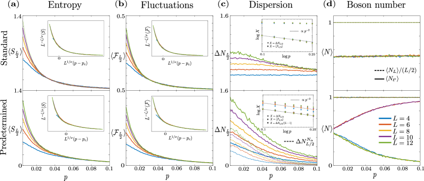
Figure 4: Numerical simulations for a transmon array in the hard-core boson limit using the standard and predetermined measurements for system sizes $L=4,6,8,10,12$. (a) von Neumann entropy and (b) Fluctuations of the number operator in the half of the chain averaged over iterations as a function of the measurement probability $p$. The insets show the finite-size scaling analysis using the Ansatz $L^{-\zeta/\nu}\braket{S/\mathcal{F}}=f[L^{-1/\nu}(p-p_{c})]$, where $p_{c}$ is the critical parameter, $\zeta$ and $\nu$ are the scaling exponents and $f[x]$ is an unknown function [houdayer04]. (c) Dispersion in the number of bosons in the half of the chain of transmons as a function of the measurement probability $p$. For the predetermined measurements we also include the dispersion in the specific total photon number sectors $N_{\overline{\alpha}}$ (light-colored dashed lines), see Eqs. (LABEL:DN_nonconserving_app) and (LABEL:DN_conserving_app) in App. LABEL:appsec:circuit_average. The insets show the comparison of the fluctuations of the number operator (diamonds) and the dispersions in the number of bosons (squares) with the $p^{-2}$ scaling (gray dashed lines) for larger values of the measurement probability. For the predetermined measurements we also show the dispersion divided by $L-1$ (stars), see Eq. (LABEL:DN_nonconserving_app) in App. LABEL:appsec:circuit_average. (d) The total boson number in the full chain $\braket{N_{L}}$ (dashed lines) and at one single site in the middle of the chain $\braket{N_{\ell^{\prime}}}$ (solid lines) as a function of the measurement probability $p$. For computing $\braket{S}$ and $\braket{\mathcal{F}}$ we considered post-selection of trajectories, while for $\braket{N}$ and $\Delta N$ we did not take into account any post-selection, see App. LABEL:appsec:numerical_simulation. The results are computed for $10^{4}$ iterations except for $L=12$, where the iteration count is $5\cdot 10^{3}$.

Once we have analytically demonstrated the utility of using predetermined measurements to define observables that contain statistical information about the system without the need for explicit post-selection, we now demonstrate this result on a specific circuit model by means of numerical simulations. The hybrid circuit is modeled by $L$ transmons that evolve unitarily under the possibility of applying non-unitary projective measurements in each position at each time step, which is performed or not depending on a measurement probability $p$ that can be related to the measurement rate $\Gamma$ introduced in the previous sections by $p=\Gamma dt$. This defines a time step in the hybrid circuit, which is repeated for $T/dt$ cycles, where $T=20\overline{J}^{-1}$ is the long time limit in which the quantities are evaluated and corresponds to the steady state. The initial state of the system is the product state $\ket{10}^{\otimes L/2}$, which has a definite total number of bosons given by $L/2$. The results shown below correspond to a chain of two-dimensional systems (qubits); the results on higher-dimensional systems in which standard measurements are used can be found in App. LABEL:appsec:numerical_simulation. All the numerical simulations were carried out without taking into account any disorder in the parameters (i.e.  $\overline{\braket{\cdot}}\to\braket{\cdot}$), thus simplifying the trajectories, which depend only on the results of the interleaved measurements performed during the time evolution.

V.1 Phase transitions in transmon arrays using different types of measurements

Figure 4 shows the main numerical results for system sizes $L=4-12$ as a function of the measurement probability using the two types of measurements for a large number of iterations of the circuit. Although all the quantities are calculated from the same set of simulations, there are crucial differences regarding post-selection. In the cases of the von Neumann entropy $\braket{S_{L/2}}$ and the fluctuations of the number operator $\braket{\mathcal{F}_{L/2}}$, we compute them for each final state of each iteration of the simulation, which are actual quantum trajectories that generally corresponds to a superposition. Then we average all the results over the iterations which, in this case, are equivalent to the trajectories. This reflects the need to account for explicit post-selection, i.e., keep track of the result of each measurement to know the exact final state, which is repeatedly measured to obtain the expected value. In the case of the boson number $\braket{N}$ and its dispersion $\Delta N$, we do not calculate any expectation value for the final states, but we emulate a real measurement by projecting the final state using Born’s rule and then averaging all these results over all iterations. This implies that each iteration is not equivalent to a real trajectory except in the cases where the final state of the trajectory is a product state, and the averaged values are obtained directly from the distribution of the results by $\textnormal{mean}[N]=\braket{N}$ and $\textnormal{var}[N]=\Delta N$, in the sense explained in Fig. 2. This implies that, if the trajectory corresponds to a superposition state, it is possible to obtain different values each time we perform the final measurement; therefore, it is not required to know the full final state to evaluate the number of bosons and its dispersion, which corresponds to the lack of need for post-selection.

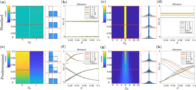
Figure 5: Boson number distributions for standard (a)-(d) and predetermined (e)-(h) measurements. (a), (e) Boson number distribution at the middle of the chain as a function of measurement probability $p$. The small panels represent the comparison of the boson number distribution with the theoretical uniform and delta distributions (solid and dashed lines) at $p=\{0.005,0.045,0.1\}$. (b), (f) The distance between the distributions with respect to theoretical uniform and delta distributions. The insets show the same analysis for the data of the sector $N_{\overline{\alpha}}$. (c), (g) The distribution of the total boson number in the full chain as a function of the measurement probability $p$. The small panels represent the comparison of the total boson number distribution with the theoretical Gaussian and delta distributions (solid and dashed lines) at $p=\{0.005,0.045,0.1\}$. (d), (h) The distance between the distributions with respect to theoretical delta and Gaussian as a function of measurement probability $p$. See App. LABEL:appsec:numerical_simulation for more details on the distributions. The results are computed for $10^{4}$ iterations except for $L=12$, where the iteration count is $5\cdot 10^{3}$.

Fig. 4(a) shows that the iteration-averaged von Neumann entropy of the half of the chain $\braket{S_{L/2}}$ has values dependent on subsystem size for small values of $p$ and collapses to the same size-independent values for a given $p_{c}$ that tending to zero, thus demonstrating the existence of a transition from a volume-law phase to an area-law phase. As expected, the collapsing behavior of the iteration-averaged fluctuation of the number operator in the half of the chain of transmons $\braket{\mathcal{F}_{L/2}}$ as a function of the measurement probability coincide with that of the von Neumann entropy [Fig. 4(b)]. The values thus obtained in the finite-size scaling analysis (figure insets) for the critical parameter $p_{c}$ and scaling exponents $\nu$ and $\zeta$ are the following: for the standard measurement, $p_{c}^{S,st}=0.022\pm 0.002$, $\nu^{S,st}=2.57\pm 0.15$, $\zeta^{S,st}=0.53\pm 0.06$ and $p_{c}^{\mathcal{F},st}=0.024\pm 0.002$, $\nu^{\mathcal{F,st}}=2.9\pm 0.2$, $\zeta^{\mathcal{F,st}}=0.50\pm 0.08$; and for the predetermined measurement, $p_{c}^{S,pre}=0.032\pm 0.003$, $\nu^{S,pre}=3.4\pm 0.2$, $\zeta^{S,pre}=0.9\pm 0.1$ and $p_{c}^{\mathcal{F},pre}=0.028\pm 0.004$, $\nu^{\mathcal{F,pre}}=3.8\pm 0.4$, $\zeta^{\mathcal{F,pre}}=1.01\pm 0.11$; for the von Neumann entropy and the fluctuation of the number operator in both cases. The analyzed systems are small, so the results of the finite-size scaling analysis should be considered approximations. In that sense, we can assume that both standard and predetermined measurements yield the same critical parameters, as one could expect, at least when there is an absorbing state [piroli2023]. However, due to the small system size, we can not rule out the possibility that the observed phase transition is a Berezinskii-Kosterlitz-Thouless (BKT) phase transition induced by the measurements rather than a canonical MIPT [alberton21]. In this case, instead of a volume-law phase, there is a sub-extensive phase where the entanglement entropy scales logarithmically with system size. This is plausible because the hard-core bosons model studied can be transformed into a free fermions model using the Jordan-Wigner transformation [Rigol2005], which is known to undergo a BKT phase transition with standard [alberton21] and predetermined [buchhold22] measurements. However, it is important to note that this issue is not trivial as the transformation introduces non-local correlations [Rigol2005] that may impact the properties of entanglement entropy (supplementary material in Ref. [alberton21]).

As predicted in App. LABEL:appsec:circuit_average, in the case of the standard measurement, the dispersion in the number of bosons in half of the chain of transmons $\Delta N_{L/2}$ as a function of $p$ does not behave similarly to the fluctuation and show a non-smooth dependency on the subsystem size [Fig. 4(c)]. In the case of the predetermined measurement, selecting the dispersion of the number of bosons of the half of the chain for the iterations with a total number of bosons $N_{\overline{\alpha}}=L/2$ [as described in Eq. (12)], there is a collapse of the curves, but it occurs for a higher measurement probability than in the case of $\braket{S_{L/2}}$ and $\braket{\mathcal{F}_{L/2}}$, being the volume-law phase overestimated and not giving useful information about the exact location of the critical point, but still proving the existence of two different phases. In the insets of Fig. 4(c), we show the comparison of $\braket{\mathcal{F}_{L/2}}$ and $\Delta N_{L/2}$ for larger measurement probabilities for the total dispersion of Eq. (11), thus representing the behavior in area-law phase. For the predetermined measurement, both quantities scale as $p^{-2}$ as predicted by the replica method for the fluctuation and by simple statistical arguments for the fluctuation and the dispersion. Interestingly, although both analytical approaches were performed at the limit of the fully measured system, the results agree with the numerical simulations for smaller measurement probabilities, but still in the area-law phase. Note that if we had considered all the iterations (thus including cases with a different total number of bosons), the dispersion scales in a similar way but with a factor $L-1$ depending on the size of the system as described in Eq. (11). The mean value of the total number of bosons $\braket{N_{L}}$ measured in the full chain of transmons results in constant values for both types of measurements [dashed lines in Fig. 4(d)], although the slight deviation in the case of the predetermined measurement demonstrates the existence of trajectories with different total numbers of bosons maintaining the same value on average, as predicted. Finally, we also show the number of bosons averaged over iterations at a single site $\braket{N_{\ell^{\prime}}}$ in the middle of the chain $\ell^{\prime}=L/2$ [solid lines in Fig. 4(c)], whose value is constant $\sim 1/2$ for the standard measurement and increases from $0$ to $1/2$ for even sites (decreases from $1$ to $1/2$ for odd sites) in the case of the predetermined measurement, agreeing quite good the result of the replica method.

V.2 Bosons number distribution indirectly diagnose the entanglement phase transition in individual trajectories for predetermined measurements

As discussed above in Fig. 4, $\braket{N}$ is not informative regarding the phase transition in either of the two measurements: $\braket{N_{L}}$ is constant in both cases and $\braket{N_{\ell^{\prime}}}$ is constant for the standard measurement and changes monotonically for the predetermined measurement, for all measurement probabilities. However, the fact that the phase transition occurs in the statistical properties of the circuit dynamics suggests studying the distribution of the measurement results of such observables, which ultimately depends on the distribution of the ground state over the Fock space [altland22]. In the area-law phase, the high measurement probability $p$ produces products states close to $\ket{\alpha_{1},\alpha_{2},...,\alpha_{L}}$, while in the volume-law phase, due to ergodicity, the stationary states will correspond to superpositions of the type of $\binom{L+N_{\rm T}-1}{N_{T}}^{-1/2}\sum_{i_{1}+i_{2}+\cdots+i_{L}=N_{T}}\ket{i_{1},i_{2},\dots,i_{L}}$ in which all states of the base vectors are visited with equal probability, where $N_{T}$ corresponds to the total number of bosons in a particular sector. Although an individual stationary state is a superposition of states belonging to the same sector, due to the presence of predetermined measurements that do not preserve the total number of bosons, different stationary states (i.e. trajectories and iterations) could belong to sectors other than the initial state. In this sense, we measure the fit of the observed distributions to the two distributions of the extreme cases $p=\{0,1\}$ for $N_{L}$ and $N_{\ell^{\prime}}$: in the area-law phase ($p=1$) there is a delta distribution corresponding to the value of the observable in the state $\ket{\alpha_{1},\alpha_{2},...,\alpha_{L}}$; and in the volume-law phase ($0<p\ll 1$) the distribution of the value of the observable corresponds to the one existing for a uniform distribution of the base vectors.

In Fig. 5 we show the numerical results regarding the distributions of the measured values of the number of bosons and their fit to two theoretical distributions for the predetermined and standard measurements. In this case, we do not consider any averaged quantity, but we take into account each of the actual measurement results for each iteration without post-selecting them (See App. LABEL:appsec:numerical_simulation for more details). In the case of $N_{\ell^{\prime}}$, the standard measurements fit the uniform distribution for all measurement probabilities [Fig. 5(a) and Fig. 5(b)], while the predetermined measurement fits a uniform distribution for small $p$ and a delta distribution for large $p$, with a crossing point between $p\sim 0.035$ and $p\sim 0.04$ [Fig. 5(e) and Fig. 5(f)]. This crossing point suggests that there is a transition between phases with different statistics in the steady states, and is in good agreement with the value of the critical parameter obtained by finite-size scaling for the iteration-averaged von Neumann entropy $p_{c}^{S,pre}=0.032\pm 0.003$. We can also compare this critical parameter with the rough estimate by the replica method $p_{c}^{d}=0.04$, which are in good agreement with the numerical results even having considered corrections only up to second order in $\overline{J}/\Gamma$ in the non-Hermitian perturbation theory. In the inset of Fig. 5(f), we show the same result for the data selected for the sector $N_{\overline{\alpha}}$, where there is a crossing point around $p\sim 0.03$.

In the case of the total number of bosons we show that for the predetermined measurement, there is an inversion in the fitting of the two distributions for different system sizes [Fig. 5(g) and Fig. 5(h)], although there is some size-dependent effect in the fittings, which should be re-scaled to locate the value of the critical parameter. Although the important result, in this case, is the existence of two phases and a transition between them, and that the volume-law phase coincides with the prediction of ergodicity based on purely theoretical arguments, that support the reasoning about replica symmetry breaking discussed in Sec. III. For the standard measurement, all trajectories have the same number of bosons, because the measurement preserves this symmetry fitting perfectly to the delta distribution [Fig. 5(c) and Fig. 5(d)].

Note that the theoretical distributions in the states yield different distributions for the number of bosons depending on the case. In the volume-law phase, the distribution for $N_{L}$ is a Gaussian centered at $N_{T}=L/2$ and uniform for $N_{\ell^{\prime}}$, but in both cases, these distributions are computed directly by considering a uniform distribution in the vectors of the basis. In the area-law phase, the distributions are $\delta_{N_{L},L/2}$ for $N_{L}$ and $\delta_{N_{\ell^{\prime}},\alpha_{\ell^{\prime}}}$ for $N_{\ell^{\prime}}$ (located at $N=0$ or $N=1$, depending on the parity of the site $\ell^{\prime}$ in the middle of the chain). This point is of utmost importance since the fact that the fitting $N_{\ell^{\prime}}$ does not change for the standard measurement does not imply an absence of a phase transition. As in the case of the predetermined measurements, the steady states are distributed uniformly over the basis states for the ergodic phase, which corresponds to a uniform distribution in the number of bosons. But in the area-law phase, we must consider the states corresponding to the $2^{L}$ eigenstates of the standard measurement so that the stationary states are uniformly distributed over the basis vectors, as in the case of the volume-law phase, yielding the same results in both phases. Note that the previous result is obtained from simple observables, which we propose indirectly coincides with the critical parameter of the entanglement transition in individual quantum trajectories. The nature of this transition is expected to be different, possibly even representing a crossover. Modifying the probability of performing a correction after each measurement shifts the critical point (data not shown), in the sense described in Refs. [odea22, ravindranath22].

VI Discussion and Conclusions

In this work, we have presented a new perspective on the experimental realization of entanglement phase transitions induced by measurements, by means of which we can have access to information about the phase in which the system is located by monitoring simple-to-measure observables without post-selecting trajectories, using quantum measurements, denoted as predetermined measurement, in which the post-measurement state is is determined in advance. For this, we have considered a superconducting circuit consisting of interacting transmons, Eq. (1), on which projective measurements are applied probabilistically, Eq. (2). To access the statistical information of the dynamics where the phase transition is observed, we have used the replica method, thus obtaining analytically an effective non-Hermitian Hamiltonian, Eq. (13), which can be interpreted as describing the dynamics of interacting bosons in an enlarged space, Eq. (14). By developing a non-Hermitian perturbation theory, Eq. (18), we have described the behavior of quantities that depend on explicit post-selection (entanglement entropy and fluctuations of the number operator) and independent of explicit post-selection (boson number), in the area-law phase for both the standard and predetermined measurements. By means of simple statistical arguments, we have also introduced a post-selection independent quantity that describes the dispersion of the boson number, which behaves similarly to the fluctuations of the numerical operator in the area law phase. Using numerical simulations, we have demonstrated the existence of a phase transition in the entanglement properties in interacting transmons, both for standard and predetermined measurements. In the case of predetermined measurements, the transition can be indirectly observed in the distribution of the number of bosons measured in a single transmon without the need to perform a post-selection of trajectories and without considering absorbing states.

The dynamics of our system, consisting of interacting transmons, can be described using the Bose-Hubbard model. It is important to note that this dynamic does not correspond to a quantum circuit in the context of quantum computing. To simplify our analysis and utilize available analytical tools like the replica method, we have designed a hybrid circuit involving unitary gates and measurements. In experimental systems, blocking the natural unitary dynamics of the system becomes necessary during measurements. This can be achieved by inhibiting the hopping interaction between the transmons, ensuring the isolation of the bosons during measurement procedures. This can be achieved either by detuning the transmon frequencies [Karamlou22] or having tunable couplers [arute2019]. Throughout the work, all the results are expressed as a function of the mean value of the hopping rate $\overline{J}$. The choice of this parameter in the experimental set determines the other parameters and critical values. These hybrid circuits are models of open quantum circuits interacting with an environment, representing the volume-law phase where the circuit is useful for computation/communication purposes. This encourages further investigation into the limit of continuous measurements, enabling the study of the Bose-Hubbard model without creating an artificial circuit. Consequently, the knowledge gained here can be applied to understand the natural dynamics of transmons as open quantum systems, aiding in comprehending the quantum-to-classical transition.

One of the biggest issues facing the experimental implementation of a MIPT is the need to perform an explicit post-selection of all the trajectories generated by the dynamics of the circuit in the different experiments in order to calculate the relevant quantities [Potter2022]. In this work, we have proposed the use of predetermined measurements to gain insight into the phase of the system without considering post-selection. These measurements consist of standard projective measurements after which we access their outcomes classically and we apply a unitary gate to bring the system to a predetermined state. This process resembles a probabilistic quantum error correction circuit, where we already know the correct state beforehand. The experimental implementation of predetermined measurements shares the same technical details as standard quantum error correction, making it relevant from an experimental standpoint. We have found through numerical simulations, and analytical analysis in the area-law phase, that fluctuations in the number operator have coinciding behavior with the entanglement entropy. This holds true for both standard and predetermined measurements. Similar outcomes have been observed in standard measurements [moghaddam2023], where fluctuations have been proven to provide an exponential shortcut compared to measuring entanglement entropy, thereby reducing the cost of post-selection.

It is also interesting to compare our results using predetermined measurements for studying simple observables with other recent works involving some sort of feedback after the measurements [buchhold22, iadecola22, odea22, ravindranath22, piotr2023, piroli2023]. In these works, the averaged density matrix undergoes an absorbing state phase transition (APT), which generally belongs to a different universality class than the MIPT occurring in the entanglement of individual quantum trajectories. Unlike our model, these works assume the existence of an absorbing state that remains unchanged under the action of the unitary circuit. Once absorbed, the state cannot change, and the timescale to reach this state reveals the APT at the critical point [piotr2023, ravindranath22, piroli2023, odea22]. In our case, there is no absorbing state since the unitary dynamics modify the state selected by the measurements; instead of a direct percolation model, we could speculate that our hybrid circuit could be cast as a classical reaction-diffusion model [hinrichsen2000], although it is not clear to which universality class it belongs. Also, the order parameter has a characteristic behavior along the APT, being constant in the absorbing phase and depending on the measurement parameter on the non-absorbing phase [piotr2023, odea22, piroli2023]. In our case, analytical and numerical results show that the order parameter quantities, e.g. the boson number at a single site, depend on the measurement probability for any non-zero probability. It is intriguing to explore whether the phase transitions in the averaged density matrix, with and without absorbing states, belong to the same universality class (and the absorbing state is not a necessary condition); or if they belong to different universality classes. Our approach eliminates the need for obtaining the averaged density matrix avoiding quantum state tomography. Additionally, by analyzing the results based on the sectors of the total number of bosons, we gain distinct and valuable information about the statistics using simple observables [Eq.(12), Fig.4(c), and the inset in Fig. 5(c)]. This suggests the possibility that the predetermined measurements include critical results for different sectors in an overlapping way.

For future work, it will be interesting to conduct numerical simulations of larger systems using tensor network methods to quantitatively examine critical parameters and scaling exponents of the phase transition and to which universality classes belong in different conditions; we still have to determine whether the hard-core bosons undergo a BKT or a MIPT phase transition. Transmons provide an ideal setting for this investigation as they allow for the modification of various parameters defining different system types. For instance, studying the effect of increasing anharmonicity, that is, on-site interactions, or introducing disorder in the Bose-Hubbard Hamiltonian parameters, which scales as $dt^{2}$ as demonstrated, could offer a more diverse range of phases [Orell2019, mansikkamaki21, yamamoto2023]. It would also be interesting to study how the dimension of the local subsystems affects the critical properties of the MIPT. Here we have seen preliminary results that arrays of two-dimensional subsystems with dimension, such as qubits or hard-core bosons, have a smaller critical parameter than the case where the dimension of the subsystem is larger in the case of standard measurements (see Fig. 4 and Fig. LABEL:fig:numerical_results_3), as predicted for qudits [bao20]. Although in transmons, the role of the anharmonicity could be non-trivially crucial as Fig. LABEL:fig:numerical_results_3(d) suggests. In our numerical simulations of higher dimensional transmons, we used a relatively large value of $U/J=5$, which is experimentally feasible, compared to the value of $U/J=0.14$ used in a similar model [tang20]. In that model, a phase transition from volume-law to area-law behavior was observed, with critical parameters close to those of random unitary circuit models [vasseur19]. Considering that our results in the limit of hard-core bosons ($U\to\infty$) possibly indicate a BKT phase transition, it would be interesting to investigate the influence of on-site interaction strength in arrays of system with higher local dimensions, that is, qudits or bosons.

Appendix A Suzuki-Trotter expansion

In this appendix we summarize the standard Suzuki-Trotter expansion procedure, after which we include a measurement layer. We will show how to create a hybrid circuit consisting of unitary evolution and interleaved probabilistic measurements, starting from a unitary Hamiltonian that describes the natural dynamics of the system. We use a Suzuki-Trotter decomposition of the Hamiltonian, Eq. (1), to design a unitary layer in terms of two-site gates [Pierkarska2018, Jaschke2018, Orell2019, Sieberer19, Barbiero2020, kargi21], and then we add a layer of measurements (in a similar way as in Ref. [tang20]), but without the necessity of considering matrix product states [vidal03]. Let us start by considering that, after a time interval $T$, the state of the system is given by

$$\ket{\psi_{T}}=e^{-i\hat{H}T}\ket{\psi_{0}},$$ (28)

where $\ket{\psi_{0}}$ is any initial state and we have made $\hat{H}/\hbar\equiv\hat{H}$. The Hamiltonian (1) can be decomposed into two terms $\hat{H}=\hat{H}_{\textnormal{odd}}+\hat{H}_{\textnormal{even}}$, where $\hat{H}_{\textnormal{odd}}\equiv\sum_{\text{odd }\ell}^{L}\hat{H}_{\ell}$ and $\hat{H}_{\textnormal{even}}\equiv\sum_{\text{even }\ell}^{L}\hat{H}_{\ell}$, and $\hat{H}_{\ell}$ is given by Ref. [vidal04]

$$\hat{H}_{\ell}\equiv\omega_{\ell}\hat{n}_{\ell}+J_{\ell}(\hat{a}_{\ell}^{\dagger}\hat{a}_{\ell+1}+h.c.)-\frac{U_{\ell}}{2}\hat{n}_{\ell}(\hat{n}_{\ell}-\hat{I}),$$ (29)

where $[\hat{H}_{\ell_{o}},\hat{H}_{\ell^{\prime}_{o}}]=[\hat{H}_{\ell_{e}},\hat{H}_{\ell^{\prime}_{e}}]=0$, for odd $(\ell_{o},\ell^{\prime}_{o})$ and even $(\ell_{e},\ell^{\prime}_{e})$ sites. Note that $[\hat{H}_{\textnormal{odd}},\hat{H}_{\textnormal{even}}]\neq 0$, but it does not affect the results [suzuki90]. Now, we can perform a Trotter expansion of order $q$ of the unitary time evolution operator $\hat{U}=e^{-i\hat{H}T}=e^{-i(\hat{H}_{\textnormal{odd}}+\hat{H}_{\textnormal{even}})T}$ for a small time step $dt>0$ such that [suzuki90]

$$\left[e^{-i(\hat{H}_{\textnormal{odd}}+\hat{H}_{\textnormal{even}})T}\right]^{T/dt}\approx\left[f_{q}\left(\hat{U}_{H_{o}dt},\hat{U}_{H_{e}dt}\right)\right]^{T/dt},$$ (30)

where $\hat{U}_{H_{o}dt}\equiv e^{-i\hat{H}_{\textnormal{odd}}dt}$, $\hat{U}_{H_{e}dt}\equiv e^{-i\hat{H}_{\textnormal{even}}dt}$ and $f_{q}(x,y)$ corresponds to the $q$ order expansion, where the first two orders are given by $f_{1}(x,y)=xy$ and $f_{2}(x,y)=x^{1/2}yx^{1/2}$.

Therefore, we can express the approximation to the evolution operator $\hat{U}=e^{-i\hat{H}T}$ as a product of $\mathcal{O}\left(T/dt\right)$ operators $\hat{U}_{H_{o}dt}$ and $\hat{U}_{H_{e}dt}$, which are constituted by the product of two-body gates

$$\hat{U}_{H_{o}dt}=\prod_{\text{odd }\ell}^{L}e^{-i\hat{H}_{\ell}dt},\quad\hat{U}_{H_{e}dt}=\prod_{\text{even }\ell}^{L}e^{-i\hat{H}_{\ell}dt}.$$ (31)

The approximation to the time evolution in (28) is obtained by applying iteratively $f_{q}(\hat{U}_{H_{o}dt},\hat{U}_{H_{e}dt})$ to $\ket{\psi_{0}}$ a number of $\mathcal{O}(T/dt)$ times (involving $\mathcal{O}(T/dt)$ times the set of gates $\hat{U}_{H_{o}dt}$ and $\hat{U}_{H_{e}dt}$). Considering $\ket{\tilde{\psi}_{t}}$ as the approximate evolved state at time $t$, the time evolution step is given by

$$\ket{\tilde{\psi}_{t+dt}}=f_{q}(\hat{U}_{H_{o}dt},\hat{U}_{H_{e}dt})\ket{\tilde{\psi}_{t}},$$ (32)

which introduces an error made by the order-$dt$ Trotter expansion (30), arising from neglecting corrections that scale as $\epsilon_{te}\sim(dt)^{2q}T^{2}$ (for an error given by $\epsilon_{te}(t)\equiv 1-|\braket{\psi_{t}}{\tilde{\psi}_{t}}|^{2}$). Finally, we add a layer of measurement operators, which are going to be applied with a probability $p$, such that the effective time step of the circuit is expressed as

$$\ket{\tilde{\psi}_{t+dt}}=\prod_{\ell}^{L}M_{\ell}(p)f_{q}(\hat{U}_{H_{o}dt},\hat{U}_{H_{e}dt})\ket{\tilde{\psi}_{t}},$$ (33)

where $M_{\ell}(p)$ represents the measurements, and $\ket{\tilde{\psi}_{t+dt}}$ needs to be renormalized after the measurements have been performed. It is important to note that the time scale $dt$ of the layer of measurements does not come from any approximation, but is set ad hoc. We are keeping just the first order in $dt$ since first and second-order Trotter expansion approximations yield the same results in the posterior analysis since the effective Hamiltonian is obtained up to first order in $dt$, in such a way the Trotter expansion errors $\epsilon_{te}$ are minimal. For the same reason, in the subsequent analysis, we would obtain the same effective Hamiltonian if we had considered $q=2$.

Appendix B Replica method

Replica method is a mathematical tool that consists of considering a number of replicas $n$ of an object describing a system (such as a partition function or a density matrix), which allows us to more easily calculate certain averaged quantities. For example, let us consider that we are interested in computing the average of the free energy of a system $\overline{F[J]}=-k_{B}T\overline{\ln Z[J]}$, where the averaging is performed over a certain distribution in $J$. In practical examples, computing $\overline{\ln Z[J]}$ can be a cumbersome task, but we can use a trick by relying on the Taylor expansion, where we introduce artificially a replica index $n$, such that the relation $\lim_{n\to 0}(Z^{n}-1)/n=\ln Z$ holds. This means that studying $(\overline{Z^{n}}-1)/n$ is analogous to studying $\overline{\ln Z}$ and in the replica limit $n\to 0$ both quantities are identical. In the present case, this method is useful since it allows us to express the von Neumann entropy as

$$\overline{S_{1}}=-\overline{\operatorname{tr}\left[\hat{\rho}\log\hat{\rho}\right]}=-\lim_{n\to 1}\frac{1}{n-1}\log\overline{\operatorname{tr}\hat{\rho}^{n}},$$ (34)

where the $n$-Rényi entropy is given by $S_{n}=\left(1-n\right)^{-1}\operatorname{tr}\hat{\rho}^{n}$ as usual. Note that we will work with a certain number of replicas, and different $n$-Rényi entropies might be thought to have different critical properties, although numerical simulations indicate that this is not the case, and they share the same critical properties [bao20].

B.1 Replicated space

Although in this article we follow the work done by Bao et al. [bao21] quite faithfully, we present below all the details of the formalism for greater clarity since we have used a slightly different notation and some details of our models differ. In the last subsection, we present the arguments for studying the effective Hamiltonian as a modified Bose-Hubbard model in an enlarged space. Since we are interested in the ensemble of trajectories of the circuit dynamics, we start by labeling states for particular sequences of measurement outcomes $m_{\bm{i}}$ and set of gate parameters $\theta_{\mathbb{i}}$ (we will refer to this sequence also as trajectory):

$$\hat{\tilde{\rho}}_{m_{\mathbb{i}},\theta_{\mathbb{i}}}(t)=\hat{P}_{m_{t}}\hat{U}_{\theta_{t}}\cdots\hat{P}_{m_{1}}\hat{U}_{\theta_{1}}\hat{\rho}_{0}\hat{U}_{\theta_{1}}^{\dagger}\hat{P}_{m_{1}}^{\dagger}\cdots\hat{U}_{\theta_{t}}^{\dagger}\hat{P}_{m_{t}}^{\dagger},$$ (35)

where $\hat{\rho}_{0}$ is the initial state, $\hat{U}_{\theta_{\mathbb{i}}}$ are the set of unitary evolution parameters, $\hat{P}_{m_{\mathbb{i}}}$ are the projection operators associated with measurement outcomes $m_{\mathbb{i}}$, and $\mathbb{i}$ refers to all the positions in the circuit space-time. The ensemble of states $\mathfrak{P}=\left\{\hat{\rho}_{m_{\mathbb{i}},\theta_{\mathbb{i}}},p_{m_{\mathbb{i}},\theta_{\mathbb{i}}}\right\}_{m_{\mathbb{i}},\theta_{\mathbb{i}}}$ is formed by the set of normalized quantum states $\hat{\rho}_{m_{\mathbb{i}},\theta_{\mathbb{i}}}\equiv\hat{\tilde{\rho}}_{m_{\mathbb{i}},\theta_{\mathbb{i}}}/p_{m_{\mathbb{i}},\theta_{\mathbb{i}}}$ and its probability distributions $p_{m_{\mathbb{i}},\theta_{\mathbb{i}}}=p_{\theta_{\mathbb{i}}}p_{m_{\mathbb{i}}}(\theta)$. The probabilities include the probability distribution for the gate parameters $p_{\theta_{\textbf{i}}}$ and the measurement outcomes probability that depends on the gate distribution parameters on the state in a sense of Born’s rule $p_{m_{\mathbb{i}}}(\theta)$. Note that the states do not need to be fully measured as in the Eq. (35), but $\mathfrak{P}$ includes also partially-measured states where we need to consider $\hat{P}_{m_{i}}=\hat{I}$ in those space-time events where no measurement was performed. Therefore, $\mathfrak{P}$ includes all possible trajectories ranging from the linear unitary trajectories with no measurements to the trajectories where all the measurements have been performed, whose proportion in the ensemble will depend on the measurement probability parameter $p$.

For studying the steady-state properties of this ensemble of states $\mathfrak{P}$, we consider the dynamics of $n$ copies of the density matrix, such that for a particular sequence of measurements and parameters, Eq. (35), the system density matrix is $\ket{\ket{\tilde{\rho}_{m_{\mathbb{i}},\theta_{\mathbb{i}}}^{(n)}}}\equiv\hat{\tilde{\rho}}_{m_{\mathbb{i}},\theta_{\mathbb{i}}}^{\otimes n}$. Similarly, we define operators acting in this replicated Hilbert space $\mathcal{H}^{(n)}=\left(\mathcal{H}\otimes\mathcal{H}^{*}\right)^{\otimes n}$, such that the unitary and measurement operators should be treated in the following way

$$\check{\mathcal{U}}_{\theta_{i}}^{(n)}\equiv(\hat{U}_{\theta_{i}}\otimes \hat{U}_{\theta_{i}}^{*})^{(n)}\to$$

$$\check{\mathcal{U}}_{\theta_{i}}^{(n)}\ket{\ket{\tilde{\rho}_{m_{\mathbb{i}},\theta_{\mathbb{i}}}^{(n)}}}\equiv(\hat{U}_{\theta_{i}}\hat{\tilde{\rho}}_{m_{\mathbb{i}},\theta_{\mathbb{i}}}\hat{U}_{\theta_{i}}^{\dagger})^{\otimes n},$$ (36)

$$\check{\mathcal{M}}_{m_{i}}^{(n)}\equiv(\hat{P}_{m_{i}} \otimes\hat{P}_{m_{i}}^{\dagger})^{(n)}\to$$

$$\check{\mathcal{M}}_{m_{i}}^{(n)}\ket{\ket{\tilde{\rho}_{m_{\mathbb{i}},\theta_{\mathbb{i}}}^{(n)}}}\equiv(\hat{P}_{m_{i}}\hat{\tilde{\rho}}_{m_{\mathbb{i}},\theta_{\mathbb{i}}}\hat{P}_{m_{i}}^{\dagger})^{\otimes n},$$ (37)

while a regular operator $\hat{O}$ (i.e., to calculate observables), acts on the state in the following way

$$\check{\mathcal{O}}^{(n)}\equiv(\hat{O}\otimes \hat{I})^{(n)}\to$$

$$\check{\mathcal{O}}^{(n)}\ket{\ket{\tilde{\rho}_{m_{\mathbb{i}},\theta_{\mathbb{i}}}^{(n)}}}\equiv(\hat{O}\hat{\tilde{\rho}}_{m_{\mathbb{i}},\theta_{\mathbb{i}}})^{\otimes n}.$$ (38)

From this point on, we will work with the un-normalized averaged state of the ensemble $\ket{\ket{\tilde{\rho}^{(n)}}}=\sum_{m_{\mathbb{i}},\theta_{\mathbb{i}}}\ket{\ket{\tilde{\rho}_{m_{\mathbb{i}},\theta_{\mathbb{i}}}^{(n)}}}=\sum_{m_{\mathbb{i}},\theta_{\mathbb{i}}}p_{m_{\mathbb{i}},\theta_{\mathbb{i}}}^{n}\ket{\ket{\rho_{m_{\mathbb{i}},\theta_{\mathbb{i}}}^{(n)}}}$, because it can be expressed as a linear function of the initial state at any time $t$, such that

$$\ket{\ket{\tilde{\rho}^{(n)}(t)}} =\sum_{m_{\mathbb{i}},\theta_{\mathbb{i}}}\ket{\ket{\tilde{\rho}_{m_{\mathbb{i}},\theta_{\mathbb{i}}}^{(n)}}}$$

$$=\sum_{m_{\mathbb{i}},\theta_{\mathbb{i}}}\check{\mathcal{M}}_{m_{t}}\check{\mathcal{U}}_{\theta_{t}}\cdots\check{\mathcal{M}}_{m_{1}}\check{\mathcal{U}}_{\theta_{1}}\ket{\ket{\hat{\tilde{\rho}}_{0}^{(n)}}}$$

$$\equiv\check{\mathcal{V}}(t)\ket{\ket{\rho_{0}^{(n)}}},$$ (39)

where the dynamics has been integrated into a linear operator $\check{\mathcal{V}}(t)$. In case of a continuous distribution for the gate parameters, we should have considered $\sum_{\theta_{\mathbb{i}}}\to\int{d\theta_{\mathbb{i}}}$. It is precisely this time evolution that we map exactly to an imaginary time evolution generated by an effective quantum Hamiltonian

$$\ket{\ket{\tilde{\rho}^{(n)}(t)}}=e^{-t\check{\mathcal{H}}_{\textnormal{eff}}}\ket{\ket{\rho_{0}^{(n)}}},$$ (40)

such that the properties of the averaged state of the ensemble $\left.\ket{\tilde{\rho}^{(n)}(t)}\right\rangle$ in the long time limit are encoded in the ground state of $\check{\mathcal{H}}_{\textnormal{eff}}$, and we have considered $\hbar=1$.

B.2 Effective Hamiltonian in the replicated space

To obtain the effective Hamiltonian in Eq. (40), we need to compute the operator $\check{\mathcal{V}}(t)$ of Eq. (39), for which we average at each space-time position $\ell^{t}\in\{1,...,M\}$ where $M=LT$. Each space-time position $\ell^{t}$ can be averaged independently, although some considerations need to be taken for averaging two-sites unitary gates. We can also average the measurement outcomes and unitary gate parameters distributions independently, obtaining $\check{\mathcal{M}}_{\ell}$ and $\check{\mathcal{U}}_{\ell}$, respectively. We assume that the gate parameters of the unitary evolution can take values from different Gaussian distributions with different mean values and variances: $\theta_{\mathbb{i}}\equiv\{\omega_{\mathbb{i}},J_{\mathbb{i}},U_{\mathbb{i}}\}$: $\left\{\overline{\omega},\sigma_{\omega}^{2}\right\}$ for the on-site energy $\omega_{\ell}$, $\left\{\overline{J},\sigma_{J}^{2}\right\}$ for the hopping strength $J_{\ell}$ and $\left\{\overline{U},\sigma_{U}^{2}\right\}$ for the interaction $U_{\ell}$. In this work we are going to consider $n=2$ replicas; to simplify the notation, we will omit the superscript $(2)$ in the following calculations. Therefore, we can perform the averaging over the circuit realizations in the following way

$$\overline{\check{\mathcal{U}}_{\ell}}= \overline{\hat{U}_{\ell}\otimes\hat{U}_{\ell}^{*}\otimes\hat{U}_{\ell}\otimes\hat{U}_{\ell}^{*}}$$

$$= \overline{e^{-i\omega_{\ell}\left(\check{\mathcal{n}}_{\ell}\right)dt}e^{-iJ_{\ell}\left(\check{\mathcal{a}}_{\ell}^{\dagger}\check{\mathcal{a}}_{\ell+1}+\check{\mathcal{a}}_{\ell}\check{\mathcal{a}}_{\ell+1}^{\dagger}\right)dt}e^{-i\frac{U_{\ell}}{2}\left(-\check{\mathcal{u}}_{\ell}\right)dt}}e^{\mathcal{O}(dt^{2})}$$

$$= \left(\frac{1}{\sqrt{2\pi\sigma_{\omega}^{2}}}\int_{-\infty}^{\infty}d\omega_{\ell}e^{-\frac{1}{2}\left(\frac{\omega_{\ell}-\overline{\omega}}{\sigma_{\omega}}\right)^{2}}e^{-i\omega_{\ell}\left(\check{\mathcal{n}}_{\ell}\right)dt}\right)\left(\frac{1}{\sqrt{2\pi\sigma_{J}^{2}}}\int_{-\infty}^{\infty}dJ_{\ell}e^{-\frac{1}{2}\left(\frac{J_{\ell}-\overline{J}}{\sigma_{J}}\right)^{2}}e^{-iJ_{\ell}\left(\check{\mathcal{a}}_{\ell}^{\dagger}\check{\mathcal{a}}_{\ell+1}+\check{\mathcal{a}}_{\ell}\check{\mathcal{a}}_{\ell+1}^{\dagger}\right)dt}\right)$$

$$\left(\frac{1}{\sqrt{2\pi\sigma_{U}^{2}}}\int_{-\infty}^{\infty}dU_{\ell}e^{-\frac{1}{2}\left(\frac{U_{\ell}-\overline{U}}{\sigma_{U}}\right)^{2}}e^{-i\frac{U_{\ell}}{2}\left(-\check{\mathcal{u}}_{\ell}\right)dt}\right)e^{\mathcal{O}(dt^{2})}$$

$$= \left(e^{-i\overline{\omega}\left(\check{\mathcal{n}}_{\ell}\right)dt-\frac{1}{2}\sigma_{\omega}^{2}\left(\check{\mathcal{n}}_{\ell}\right)^{2}dt^{2}}\right)\left(e^{-i\overline{J}\left(\check{\mathcal{a}}_{\ell}^{\dagger}\check{\mathcal{a}}_{\ell+1}+\check{\mathcal{a}}_{\ell}\check{\mathcal{a}}_{\ell+1}^{\dagger}\right)dt-\frac{1}{2}\sigma_{J}^{2}\left(\check{\mathcal{a}}_{\ell}^{\dagger}\check{\mathcal{a}}_{\ell+1}+\check{\mathcal{a}}_{\ell}\check{\mathcal{a}}_{\ell+1}^{\dagger}\right)^{2}dt^{2}}\right)$$

$$\left(e^{-i\frac{1}{2}\overline{U}\left(-\check{\mathcal{u}}_{\ell}\right)dt-\frac{1}{8}\sigma_{U}^{2}\left(-\check{\mathcal{u}}_{\ell}\right)^{2}dt^{2}}\right)e^{\mathcal{O}(dt^{2})}$$

$$= e^{-i\check{\mathcal{A}}_{\ell}dt-\check{\mathcal{B}}_{\ell}dt^{2}}e^{\mathcal{O}(dt^{2})},$$ (41)

where the operators of the replicated space are given by

$$\check{\mathcal{A}}_{\ell} =\overline{\omega}\check{\mathcal{n}}_{\ell}+\overline{J}(\check{\mathcal{a}}_{\ell}^{\dagger}\check{\mathcal{a}}_{\ell+1}+\check{\mathcal{a}}_{\ell}\check{\mathcal{a}}_{\ell+1}^{\dagger})-\frac{1}{2}\overline{U}\check{\mathcal{u}}_{\ell},$$ (42)

$$\check{\mathcal{B}}_{\ell} =\frac{1}{2}\sigma_{\omega}^{2}\left(\check{\mathcal{n}}_{\ell}\right)^{2}+\frac{1}{2}\sigma_{J}^{2}(\check{\mathcal{a}}_{\ell}^{\dagger}\check{\mathcal{a}}_{\ell+1}+\check{\mathcal{a}}_{\ell}\check{\mathcal{a}}_{\ell+1}^{\dagger})^{2}+\frac{1}{8}\sigma_{U}^{2}\left(\check{\mathcal{u}}_{\ell}\right)^{2},$$ (43)

$$\check{\mathcal{n}}_{\ell} =\hat{n}_{\ell}\hat{I}\hat{I}\hat{I}-\hat{I}\hat{n}_{\ell}\hat{I}\hat{I}+\hat{I}\hat{I}\hat{n}_{\ell}\hat{I}-\hat{I}\hat{I}\hat{I}\hat{n}_{\ell},$$ (44)

$$\check{\mathcal{u}}_{\ell} =[\hat{n}_{\ell}(\hat{n}_{\ell}-\hat{I})]\hat{I}\hat{I}\hat{I}-\hat{I}[\hat{n}_{\ell}(\hat{n}_{\ell}-\hat{I})]\hat{I}\hat{I}+\hat{I}\hat{I}[\hat{n}_{\ell}(\hat{n}_{\ell}-\hat{I})]\hat{I}-\hat{I}\hat{I}\hat{I}[\hat{n}_{\ell}(\hat{n}_{\ell}-\hat{I})],$$ (45)

$$\check{\mathcal{a}}_{\ell}^{\dagger}\check{\mathcal{a}}_{\ell+1} =(\hat{a}_{\ell}^{\dagger}\hat{I}\hat{I}\hat{I})(\hat{a}_{\ell+1}\hat{I}\hat{I}\hat{I})-(\hat{I}\hat{a}_{\ell}^{\dagger}\hat{I}\hat{I})(\hat{I}\hat{a}_{\ell+1}\hat{I}\hat{I})+(\hat{I}\hat{I}\hat{a}_{\ell}^{\dagger}\hat{I})(\hat{I}\hat{I}\hat{a}_{\ell+1}\hat{I})-(\hat{I}\hat{I}\hat{I}\hat{a}_{\ell}^{\dagger})(\hat{I}\hat{I}\hat{I}\hat{a}_{\ell+1}),$$ (46)

$$\check{\mathcal{a}}_{\ell}\check{\mathcal{a}}_{\ell+1}^{\dagger} =(\hat{a}_{\ell}\hat{I}\hat{I}\hat{I})(\hat{a}_{\ell+1}^{\dagger}\hat{I}\hat{I}\hat{I})-(\hat{I}\hat{a}_{\ell}\hat{I}\hat{I})(\hat{I}\hat{a}_{\ell+1}^{\dagger}\hat{I}\hat{I})+(\hat{I}\hat{I}\hat{a}_{\ell}\hat{I})(\hat{I}\hat{I}\hat{a}_{\ell+1}^{\dagger}\hat{I})-(\hat{I}\hat{I}\hat{I}\hat{a}_{\ell})(\hat{I}\hat{I}\hat{I}\hat{a}_{\ell+1}^{\dagger}).$$ (47)

Note that expressions for the operators have been simplified $\check{\mathcal{O}}=\hat{O}_{1}\otimes\hat{O}_{2}\otimes\hat{O}_{3}\otimes\hat{O}_{4}\equiv\hat{O}_{1}\hat{O}_{2}\hat{O}_{3}\hat{O}_{4}$, where $\hat{O}_{i}$ and $\check{\mathcal{O}}$ are $d$-dimensional and $d^{4}$-dimensional operators, respectively, and should be understood in the sense of Eq. (38). In what follows, we will describe all the relevant steps followed in Eq. (41). In the first step, we have taken into account that $e^{\hat{A}}\otimes e^{\hat{B}}=e^{\hat{A}\otimes\hat{I}+\hat{I}\otimes\hat{B}}$; note that the operators defined in (29) include the four terms, each acting on different Hilbert spaces, i.e. they commute. Note that some of the replicated operators do not commute between them: $[\check{\mathcal{n}}_{\ell},\check{\mathcal{a}}_{\ell}^{\dagger}\check{\mathcal{a}}_{\ell+1}+\check{\mathcal{a}}_{\ell}\check{\mathcal{a}}_{\ell+1}^{\dagger}]\neq 0$ and $[\check{\mathcal{u}}_{\ell},\check{\mathcal{a}}_{\ell}^{\dagger}\check{\mathcal{a}}_{\ell+1}+\check{\mathcal{a}}_{\ell}\check{\mathcal{a}}_{\ell+1}^{\dagger}]\neq 0$. Therefore, we have consider that $e^{\hat{A}dt+\hat{B}dt+\hat{C}dt}=e^{\hat{A}dt}e^{\hat{B}dt}e^{\hat{C}dt}e^{\mathcal{O}(dt^{2})}$, where the term $e^{\mathcal{O}(dt^{2})}$ includes all the commutators of order $dt^{2}$ arising from the Baker-Campbell-Hausdorff (BCH) formula. In the second step, we perform a standard Gaussian integration considering the means and variances of the different parameters, and that for each integration the operators commute with themselves. In the last step, we consider again the BCH formula and group all the $\mathcal{O}(dt^{2})$ terms in $e^{\mathcal{O}(dt^{2})}$. Note that, since the following commutators vanish $[(\check{\mathcal{n}}_{\ell}+\check{\mathcal{n}}_{\ell+1})^{2},(\check{\mathcal{a}}_{\ell}^{\dagger}\check{\mathcal{a}}_{\ell+1}+\check{\mathcal{a}}_{\ell}\check{\mathcal{a}}_{\ell+1}^{\dagger})^{2}]$, $[(\check{\mathcal{n}}_{\ell}+\check{\mathcal{n}}_{\ell+1})^{2},\check{\mathcal{a}}_{\ell}^{\dagger}\check{\mathcal{a}}_{\ell+1}+\check{\mathcal{a}}_{\ell}\check{\mathcal{a}}_{\ell+1}^{\dagger}]$ and $[\check{\mathcal{n}}_{\ell}+\check{\mathcal{n}}_{\ell+1},(\check{\mathcal{a}}_{\ell}^{\dagger}\check{\mathcal{a}}_{\ell+1}+\check{\mathcal{a}}_{\ell}\check{\mathcal{a}}_{\ell+1}^{\dagger})^{2}]$, it is true that $e^{\mathcal{O}(dt^{2})}=I$ if there is no interactions (i.e. $U_{\ell}=0$) and we make the change $\check{\mathcal{n}}_{\ell}\to\frac{1}{2}(\check{\mathcal{n}}_{\ell}+\check{\mathcal{n}}_{\ell+1})$. This implies that $\overline{\check{\mathcal{U}}_{\ell}(U_{\ell}=0)}=e^{-i\hat{A}_{\ell}dt-\hat{B}_{\ell}dt^{2}}$, and we can have a better physical interpretation of how the variance in the distribution of parameters will affect the subsequent analysis; in the case of $U_{\ell}\neq 0$ the result is (41), where the terms involving the variance of the parameters are of the same order as a complicate term involving different commutators, and the interpretation is less clear. It is important to note that to study the $dt^{2}$ terms properly, we need to perform the Trotter expansion up to second order (i.e. considering $q=2$ and $f_{2}(x,y)=x^{1/2}yx^{1/2}$). Interestingly, non-disorder systems yield the same result up to the first order without requiring a Trotter expansion.

For the average over the measurement results, we define the following operators, which include the average over the possible outcomes,

$$\braket{\check{\mathcal{M}}_{\ell}}=\left(1-\Gamma_{\ell}dt\right)\check{\mathcal{I}}+\Gamma_{\ell}dt\sum_{m_{\ell}}^{d}\check{\mathcal{P}}_{m_{\ell}},$$ (48)

where $\Gamma_{\ell}$ may be viewed as the rate at which a measurement of a certain type is performed, $\check{\mathcal{I}}=\hat{I}\hat{I}\hat{I}\hat{I}$, $\check{\mathcal{P}}_{m_{\ell}}=\hat{P}_{m_{\ell}}\hat{P}_{m_{\ell}}^{\dagger}\hat{P}_{m_{\ell}}\hat{P}_{m_{\ell}}^{\dagger}$ and $\hat{P}_{m_{\ell}}$ are the projectors. As discussed in App. A, we introduce ad hoc the factor $dt$, but it does not derive from any Trotter expansion as the one of the Bose-Hubbard Hamiltonian.

Finally, we obtain the transfer matrix between the state of the system at $t+dt$ and $t$ by averaging the time evolution over the gate parameters and the probabilities $p=\Gamma dt$ of applying measurement operators. For this, we only need to average over the different sites in space $\ell\in L$ for a single time $t$, i.e. just the elements from a time step,