GAT: Guided Adversarial Training with Pareto-optimal Auxiliary Tasks

Abstract

While leveraging additional training data is well established to improve adversarial robustness, it incurs the unavoidable cost of data collection and the heavy computation to train models. To mitigate the costs, we propose Guided Adversarial Training (GAT), a novel adversarial training technique that exploits auxiliary tasks under a limited set of training data. Our approach extends single-task models into multi-task models during the min-max optimization of adversarial training, and drives the loss optimization with a regularization of the gradient curvature across multiple tasks. GAT leverages two types of auxiliary tasks: self-supervised tasks, where the labels are generated automatically, and domain-knowledge tasks, where human experts provide additional labels. Experimentally, GAT increases the robust AUC of CheXpert medical imaging dataset from 50% to 83% and On CIFAR-10, GAT outperforms eight state-of-the-art adversarial training and achieves 56.21% robust accuracy with Resnet-50. Overall, we demonstrate that guided multi-task learning is an actionable and promising avenue to push further the boundaries of model robustness.

1 Introduction

Despite their impressive performance, Deep Neural Networks (DNNs) are sensitive to small, imperceptible perturbations in the input. The resulting adversarial inputs raise multiple questions about the robustness of such systems, especially in safety-critical domains such as autonomous driving (Cao et al., 2019), financial services (Ghamizi et al., 2020), and medical imaging (Ma et al., 2021).

Adversarial training (AT) (Madry et al., 2017a) is the de facto standard for building robust models. In its simplest form, AT trains the model with the original training data and adversarial examples crafted from them. Robustness can be further increased with additional data in the AT process, including unlabeled data (Carmon et al., 2019), augmented data (Rebuffi et al., 2021), or artificial data from generative models (Gowal et al., 2021). These approaches produce significantly more robust models (e.g. ResNet50 with 51.56% robust accuracy on CIFAR-10) and can be further enhanced through the use of very large models (WideResNet-70-16 with 66% robust accuracy) (Croce et al., 2020).

However, the robustness achieved by AT with data augmentation has already reached a plateau (Schmidt et al., 2018; Gowal et al., 2021) whereas the computational costs of AT in large models prohibit their use at scale. This is why research has explored new techniques to increase robustness, taking inspiration from, e.g., Neural Architecture Search  (Ghamizi et al., 2019; Dong & Yang, 2019) and self-supervised learning (Hendrycks et al., 2019; Chen et al., 2020). They are, however, not yet competitive to data augmentation techniques in terms of clean and robust performances.

In this paper, we propose Guided Adversarial Training (GAT), a new technique based on multi-task learning to improve AT. Inspired from preliminary investigations of robustness in multi-task models Mao et al. (2020) and Ghamizi et al. (2021), we demonstrate that robustness can be improved by adding auxiliary tasks to the model and introducing a gradient curvature minimization and a multi-objective weighting strategy into the AT optimization process. Our novel regularization can achieve optimal pareto-fronts across the tasks for both clean and robust performances. To this end, GAT can exploit both self-supervised tasks without human intervention (e.g. image rotation) and domain-knowledge tasks using human-provided labels.

Our experiments demonstrate that GAT outperforms eight state-of-the-art AT techniques based on data augmentation and training optimization, with an improvement on CIFAR-10 of 3.14% to 26.4% compared to state of the art adversarial training with data-augmentation. GAT shines in scarce data scenarios (e.g. medical diagnosis tasks), where data augmentation is not applicable.

Our large study across five datasets and six tasks demonstrates that task augmentation is an efficient alternative to data augmentation, and can be key to achieving both clean and robust performances.

Our algorithm and replication packages are available on https://github.com/yamizi/taskaugment

2 Background

2.1 Multi-task learning (MTL)

MTL leverages shared knowledge across multiple tasks to learn models with higher efficiency (Vandenhende et al., 2021; Standley et al., 2020a). A multi-task model is commonly composed of an encoder that learns shared parameters across the tasks and a decoder part that branches out into task-specific heads.

We can view MTL as a form of inductive bias. By introducing an inductive bias, MTL causes a model to prefer some hypotheses over others (Ruder, 2017). MTL effectively increases the sample size we are using to train our model. As different tasks have different noise patterns, a model that learns two tasks simultaneously can learn a more general representation. Learning task A alone bears the risk of overfitting to task A, while learning A and B jointly enables the model to obtain a better representation (Caruana, 1997).

2.2 Adversarial robustness

An adversarial attack is the process of intentionally introducing perturbations on the inputs of a model to cause the wrong predictions. One of the earliest attacks is the Fast Gradient Sign Method (FGSM) (Goodfellow et al., 2014a). It adds a small perturbation $\delta$ to the input of a neural network, which is defined as: $\eta=\epsilon\,\text{sign}(\delta_{x}\mathscr{L}(\theta,x,y))$, where $\theta$ are the parameters of the network, $x$ is the input data, $y$ is its associated label, $\mathscr{L}_{\theta}(x,y)$ is the loss function used, and $\epsilon$ is the strength of the attack.

Following Goodfellow et al. (2014a), other attacks were proposed, such as by adding iterations (I-FGSM) (Kurakin et al., 2016), projections and random restart (PGD) (Madry et al., 2017b), and momentum (MIM) (Dong et al., 2018).

Given a multi-task model $\mathscr{M}_{\theta}$ parameterized by $\theta$ for $M$ tasks, an input example $x$, and its corresponding ground-truth label $\bar{y}$, the attacker seeks the perturbation $\delta$ that will maximize the joint loss $\mathscr{L}_{\theta}$ of the attacked tasks:

$$\underset{\delta\in\Delta}{\operatorname{argmax}}\>\mathscr{L}_{\theta}(x+\delta,\bar{y})\>\text{s.t.}\>||\delta||_{p}\leq\epsilon,$$ (1)

where $p\in\{1,2,\infty\}$ and $\|\cdot\|_{p}$ denotes the $\ell_{p}$-norm. A typical choice for a perturbation space is to take $\Delta=\{\delta:\|\delta\|_{\infty}\leq\epsilon\}$ for some $\epsilon>0$.

$\mathscr{L}_{\theta}(x+\delta,\bar{y})=\sum_{j=1}^{M}\mathscr{L}_{j}(x+\delta,y_{j})$ is the joint loss of the M attacked tasks.

Adversarial training (AT)

AT is a method for learning networks which are robust to adversarial attacks. Given a multi-task model $\mathscr{M}_{\theta}$ parameterized by $\theta$, a dataset $\{(x_{i},y_{i})\}$, a loss function $\mathscr{L}_{\theta}$, and a perturbation space $\Delta$ , the learning problem is cast as the following optimization:

$$\min_{\theta}\sum_{i}\max_{\delta\in\Delta}\mathscr{L}_{\theta}(x_{i}+\delta,y_{i})$$ (2)

The procedure for AT uses some adversarial attack to approximate the inner maximization over $\Delta$, followed by some variation of gradient descent on the model parameters $\theta$.

2.3 Adversarial vulnerability

Simon-Gabriel et al. (2019) introduced the concept of adversarial vulnerability to evaluate and compare the robustness of single-task models and settings. Mao et al. (2020) extended it to multi-task models as follows:

Definition 2.1.

Let $\mathscr{M}$ be a multi-task model, $\mathscr{T}^{\prime}\subseteq\mathscr{T}$ be a subset of its tasks, and $\mathcal{L}_{\mathscr{T}^{\prime}}$ be the joint loss of tasks in $\mathscr{T}^{\prime}$. Then, we denote by $\mathbb{E}_{x}[\delta\mathcal{L}(\mathscr{T}^{\prime},\epsilon)]$ the adversarial vulnerability of $\mathscr{M}$ on $\mathscr{T}^{\prime}$ to an $\epsilon$-sized $\|.\|_{p}$-attack, and define it as the average increase of $\mathcal{L}_{\mathscr{T}^{\prime}}$ after attack over the whole dataset:

$$\mathbb{E}_{x}[\delta\mathcal{L}(\mathscr{T}^{\prime},\epsilon)]=\\ \mathbb{E}_{x}\left[\max_{\|\delta\|_{p}\leq\epsilon}\mid\mathcal{L}_{\mathscr{T}^{\prime}}(x+\delta,\bar{y})-\mathcal{L}_{\mathscr{T}^{\prime}}(x,\bar{y})\mid\right]$$

This definition matches the definitions of previous work (Goodfellow et al., 2014b; Sinha et al., 2017) of the robustness of deep learning models: the models are considered vulnerable when a small perturbation causes a large average variation of the joint loss.

Similarly, the adversarial task vulnerability of a task $i$ is the average increase of $\mathcal{L}_{\mathscr{T}^{\prime}}(x,y_{i})$ after attack.

3 Preliminaries

To build our method, we first investigate the factors that influence the robustness of multi-task models. This preliminary study enables us to derive relevant metrics to optimize during the AT process for multi-task models.

Our idea stems from previous observations that task weights can have a significant impact on the robustness of multi-task models (Ghamizi et al., 2022). We pursue this investigation and identify the three main factors of adversarial vulnerability in multi-task models: The relative orientation of the gradient of the tasks’ loss, their magnitude similarity and the weighting of the clean and adversarial contributions to the loss (Proof in Appendix A.1).

Theorem 3.1.

Consider a multi-task model $\mathscr{M}$ where an attacker targets $\mathscr{T}=\{t_{1},t_{2}\}$ two tasks weighted with $\alpha_{1}$ and $\alpha_{2}$ respectively, with an $\epsilon$-sized $\|.\|_{p}$-attack. If the model is converged, and the gradient for each task is i.i.d. with zero mean and the tasks are correlated, the adversarial vulnerability of the model can be approximated as

$$\mathbb{E}_{x}[\delta\mathcal{L}^{\prime}]\propto\sqrt{1+2\frac{\alpha_{1}.\alpha_{2}.\operatorname{Cov}\left(\partial_{x}\mathcal{L}_{1},\partial_{x}\mathcal{L}_{2}\right)}{\alpha_{1}^{2}\sigma_{1}^{2}+\alpha_{2}^{2}\sigma_{2}^{2}}},$$ (3)

where $\sigma_{i}^{2}=\operatorname{Cov}\left(\partial_{x}\mathcal{L}_{i},\partial_{x}\mathcal{L}_{i}\right)$ and $\partial_{x}\mathcal{L}(x,y_{i})$ the gradient of the task $i$.

The above theorem reveals that adversarial vulnerability is particularly sensitive to the relative amplitude of the gradients of the tasks and their orientation. In standard multi-task learning (MTL), the relative properties of the task gradients – such as the orientation angle, magnitude similarity, and curvature – have an impact on the learning speed and on the achieved clean accuracy (Vandenhende et al., 2021). Therefore, task weighting approaches like Projecting Conflicting Gradients (PCG) (Yu et al., 2020) rely on these properties to optimize standard training.

3.1 Empirical study

To confirm empirically the findings of Theorem 3, we study the following metrics and empirically check their correlation to robustness.

Definition 3.2.

Let $\phi_{ij}$ be the angle between two tasks’ gradients $\mathbf{g}_{i}$ and $\mathbf{g}_{j}$. We define the gradients as conflicting when $\cos\phi_{ij}<0$.

Definition 3.3.

The gradient magnitude similarity between two gradients $\mathbf{g}_{i}$ and $\mathbf{g}_{j}$ is $\Phi(\mathbf{g}_{i},\mathbf{g}_{j})=\frac{2\|\mathbf{g}_{i}\|_{2}\|\mathbf{g}_{j}\|_{2}}{\|\mathbf{g}_{i}\|_{2}^{2}+\|\mathbf{g}_{j}\|_{2}^{2}}.$

When the magnitude of two gradients is the same, this value equals 1. As the gradient magnitude difference increases, the similarity goes towards zero.

Definition 3.4.

The multi-task curvature bounding measure between two gradients $\mathbf{g}_{i}$ and $\mathbf{g}_{j}$ is $\xi(\mathbf{g}_{i},\mathbf{g}_{j})=(1-\cos^{2}\phi_{ij})\frac{\|\mathbf{g}_{i}-\mathbf{g}_{j}|_{2}^{2}}{\|\mathbf{g}_{i}+\mathbf{g}_{j}\|_{2}^{2}}.$

The multi-task curvature bounding measure combines information about both the orientation of the gradients of the tasks and the relative amplitude of the gradients.

We evaluate in Fig. 1 the Pearson correlation coefficient between the robust accuracy and each of the three metrics. For adversarially trained models (top), both the Gradient multi-task curvature bounding measure (left) and the Gradient cosine angle (right) are strongly negatively correlated with the adversarial robustness, with respectively a correlation coefficient $r$ of $-0.86$ and $-0.87$. However, for models trained with standard training, only the Gradient multi-task curvature bounding measure is negatively correlated ($r=-0.45$) to the robustness of the models.

These results show that the gradient curvature measure can be a good surrogate to study the robustness of MTL models, especially with AT. The negative correlation between the gradient curvature measure and the robust accuracy suggests that a flatter multitask loss landscape leads to more robust models. Our results are in coherence with the seminal works from Engstrom et al. (2017) and Moosavi-Dezfooli et al. (2018) studied in the single-task setting.

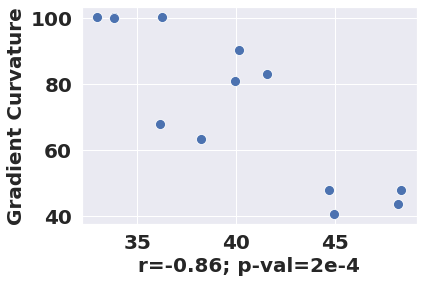
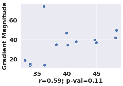
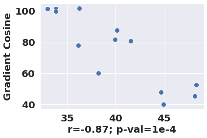
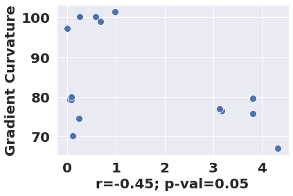
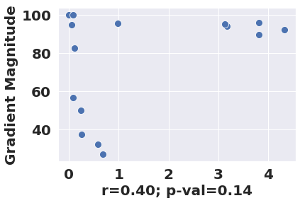
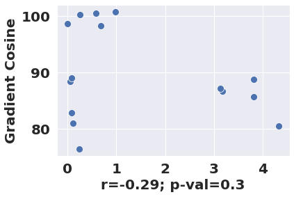
Figure 1: Robust accuracy (X-axis) with each of our three metrics (Y-axis). Top: Models with AT, bottom: Models with standard training. Left: Gradient multi-task curvature bounding measure, middle: Gradient magnitude similarity, right: Gradient cosine angle. Below each scatter plot is the Pearson correlation coefficient r and its p-value between the robust accuracy and the studied metric. This study confirms that the Gradient Curvature is a good surrogate for adversarial robustness and can be used to optimize the robustness.

4 Method

Based on our preliminary findings, we propose GAT – Guided Adversarial Training – as a new approach for effective AT. GAT introduces three novel components: (1) a multi-task AT using both self-supervised and domain-knowledge tasks, (2) a gradient curvature regularization that guides the AT towards less vulnerable loss landscapes, and (3) a pareto-optimal multi-objective optimization of the weights of each loss (clean and robust losses for target tasks) at each step of the min-max optimization of AT.

4.1 The proposed approach: GAT

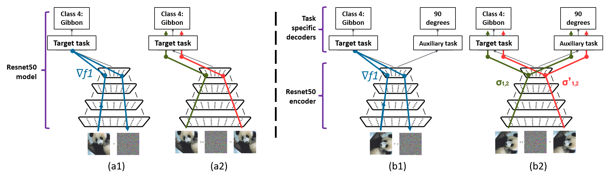
Figure 2: Comparison of single-task AT (a) and our proposed approach GAT (b). GAT preserves the original target task and adds an auxiliary task where abundant labels are available: For instance, a self-supervised task like rotation angle prediction. In (a1) and (b1), we generate the adversarial example using only the loss of the target task (blue line). We update the models’ weights with backpropagation in (a2) and (b2). We compute the model’s weights update with GAT (b2) using a weighted combination ($\sigma_{1,2},\sigma^{\prime}_{1,2}$) of the loss of the different tasks over the clean examples (green line) and the adversarial examples (red line).

GAT first transforms any single-task model into a multi-task model before AT. We connect additional decoders to the penultimate layer of the existing model. The architecture of each decoder is selected for one auxiliary task specifically. For example, we use a single dense layer as a decoder for classification tasks and a U-net (Ronneberger et al., 2015) decoder for segmentation tasks. In Figure 2, we extend an ImageNet classification model into a multi-task model that learns both the class (target task) and the orientation (auxiliary task) of the image. The auxiliary task here is ’the rotation angle prediction’, a self-supervised classification task where we can generate the labels on the fly by rotating the original image.

We consider two types of task augmentation. In self-supervised task augmentation, the image is pre-processed with some image transformation like jigsaw scrambling (Noroozi & Favaro, 2016) or image rotation (Gidaris et al., 2018). The auxiliary task predicts the applied image transformation (e.g., the permutation matrix for the jigsaw task, the rotation angle for the rotation task). In domain-knowledge tasks, a human oracle provides additional labels. In the medical imaging case, these additional labels may include, e.g., other pathologies and stages or patient data like gender and age.

A naive implementation of AT (Eq. (2)) to multi-task models consists of the following min-max optimization problem:

$$\min_{\theta}\sum_{i}\max_{\delta\in\Delta}\sum_{j=1}^{M}(\mathscr{L}_{j}(x_{i},y_{i,j})+\mathscr{L}_{j}(x_{i}+\delta,y_{i,j})),$$ (4)

where $y_{i,j}$ is the label of the input example $i$ for the task $j$.

4.2 Guiding the gradient curvature with regularization

We showed in Section 3 that the curvature bounding measure is a reliable surrogate of the adversarial robustness of models. Hence, we guide the AT of Eq. (4) with a curvature regularization term:

$$\mathscr{L}_{j}^{\mathrm{(reg)}}=\sum_{k=1}^{j-1}(1-\cos^{2}\phi_{jk})\frac{\|\mathbf{g}_{j}-\mathbf{g}_{k}|_{2}^{2}}{\|\mathbf{g}_{j}+\mathbf{g}_{k}\|_{2}^{2}}.$$

Therefore, the definitive formulation of GAT:

$$\begin{array}[]{l}\min_{\theta}\sum_{i}\max_{\delta\in\Delta}\sum_{j=1}^{M}\\ \left(\alpha_{j}^{\mathrm{(clean)}}\mathscr{L}_{j}(x_{i},y_{i,j})+\alpha_{j}^{\mathrm{(adv)}}\mathscr{L}_{j}(x_{i}+\delta,y_{i,j})+\mathscr{L}_{j}^{\mathrm{(reg)}}\right)\par\end{array}$$ (5)

where $\alpha_{j}^{\mathrm{(clean)}}$ and $\alpha_{j}^{\mathrm{(adv)}}$ are positive weights that control the relative contribution of the clean and adversarial loss (respectively) of task $j$ to the objective function to optimize. Their value will be optimized automatically throughout the AT process, as proposed below.

4.3 Adversarial Training as a multi-objective optimization problem (MOOP)

The optimization proposed in Eq. (5) faces conflicting gradients between the clean and adversarial losses, and possibly between the target and auxiliary tasks. Weighting strategies for MTL (Liu et al., 2021; Yu et al., 2020; Wang et al., 2020) all assume that the tasks’ gradients are misaligned and not totally opposed. The case of GAT is more complex because there is no guarantee that this assumption holds across the AT optimization. Instead of achieving the minimization of the whole loss, we seek to reach a Pareto-stationary point where we cannot improve the loss of one task without degrading the loss of another task (Kaisa, 1999).

To solve this MOOP, we extend the Multi-Gradient Descent Algorithm (MGDA) (Desideri, 2012) to AT. We generalize gradient descent to multi-objective settings by identifying a descent direction common to all objectives (i.e., clean and robust losses of target tasks) and tune the weights of the tasks’ losses at each adversarial training batch. MGDA formally guarantees convergence to a Pareto-stationary point (Desideri, 2012) to achieve both clean and robust performances. Subsequent research by Sener & Koltun (2018) has shown that the Multi-Gradient Descent Algorithm (MGDA) ”yields a Pareto optimal solution under realistic assumptions”. We rely on these assumptions and the upper bound they propose using the Frank-Wolfe-based optimizer (Algorithm 3) to achieve Pareto optimality. The only assumption we use is the same as the one proven by Sener & Koltun (2018), namely, the non-singularity assumption. The assumption is reasonable because the singularity implies that tasks are linearly related, and a trade-off is not necessary. Our empirical study in section 3.1 confirms that our tasks are not linearly related.

Algorithm 1 presents GAT and is explained in details (including the MGDA procedure) in Appendix A.3.

Algorithm 1 Pseudo-Algorithm of GAT

  Given: a single task model $\mathscr{M}$ parameterized by $\theta^{s}$ for the shared encoder and $\theta^{t}$ for the specific heads, a batch example $x$, and $\bar{y}=(y_{1},...,y_{s},...y_{m})$ its corresponding labels for each task, with $y_{1}$ the target task, $y_{1<i\leq s}$ the auxiliary self-supervised tasks and $y_{s<i\leq m}$ the auxiliary domain-knowledge tasks;

  Given: an input processing $f_{t}$ for each auxiliary self-supervised $t$ task with label $y_{1<t\leq s}$.

  Given: a $PGD$ adversarial attack with a step size $\epsilon_{step}$; a maximum perturbation $\epsilon$; $S$ number of attack iterations;

  Step 1: Create a decoder $D_{i}$ at the penultimate layer of $\mathscr{M}$ for each of the auxiliary task $t_{i}$ / $i>1$.

  Step 2: For each epoch and batch $x$ Do

1. For each self-supervised task $t_{1<i\leq s}$:
   $x\leftarrow\operatorname*{\bigcirc}_{t=2}^{s}\ f_{t}(x)$

2. $\hat{x}\leftarrow\mathrm{PGD}(x,y_{1},\epsilon_{step},\epsilon,S)$.

3. Get the task losses $l$ and regularization losses $l^{(reg)}$:
   $l\leftarrow l_{1,x},l_{1,\hat{x}},\ldots,l_{M,x},l_{M,\hat{x}},l^{(reg)}_{M+1,x},\ldots,l^{(reg)}_{2M-1,x}$.

4. $\alpha_{1},\ldots,\alpha_{2M-1}\leftarrow$ MGDA($\theta$,$l$)

5. $\theta^{s}\leftarrow\theta^{s}-\eta\sum_{t=1}^{2M-1}\alpha_{t}\nabla_{\theta^{sh}}l_{t,x}(\theta^{s},\theta^{t})$

  Step 3: Disable the auxiliary branches added at step 1.

5 Experiments

We extensively evaluate GAT on two datasets and demonstrate that GAT achieves better robust performances than SoTA data augmentation AT: We compare GAT with Cutmix (Yun et al., 2019), MaxUp (Gong et al., 2020), unlabeled data augmentation (Carmon et al., 2019), denoising diffusion probabilistic models augmentations (DDPM) (Gowal et al., 2021), self-supervised pre-training (Chen et al., 2020), self-supervised multi-task learning (Hendrycks et al., 2019). We also compare GAT to three popular AT approaches that do not focus on data augmentation: Madry adversarial training (Madry et al., 2017b), TRADES adversarial training (Zhang et al., 2019), and FAST adversarial training (Wong et al., 2020).

The extension of our evaluation to different settings is discussed in Section 7.

5.1 Experimental setup

We present below our main settings. Further details are in Appendix A.4.

Datasets.

CIFAR-10 (Krizhevsky et al., 2009) is a 32x32 color image dataset. We evaluate two scenarios: A full 50.000 image AT scenario and an AT scenario using a subset of 10% to simulate scarce data scenarios. A study with 25%, and 50% of the original data is in the Appendix B.1.

CheXpert (Irvin et al., 2019) is a public chest X-ray dataset. It consists of 512x512 grayscale image radiography collected from one hospital. We report below the results for predicting the Edema and the Atelectasis disease as target tasks, and provide results for other combinations of pathologies in Appendix B.2. We confirm our results for another medical imaging dataset (NIH) in Appendix C.2.

Architecture.

We use an encoder-decoder image classification architecture, with ResNet-50v2 as encoders for the main study. We provide in Appendix C complementary studies with WideResnet28 encoders.

Task augmentations.

For both CIFAR-10 and CheXpert datasets, we evaluate two self-supervised tasks: Jigsaw, where we split the images into 16 chunks and scramble them according to a permutation matrix. The permutation matrix represents the labels of the Jigsaw prediction task. In the Rotation auxiliary task, we rotate the images by 0, 90, 180, or degrees, and the 4 rotation angles are the labels learned by the Rotation prediction task.

To evaluate domain-knowledge tasks, we generate new labels as follows. For CIFAR-10, we split the existing 10 classes into 2 macro classes: Vehicles or Animals. We refer to this task as Macro. For CheXpert, we add the binary classification of Cardiomegaly and Pneumothorax as auxiliary tasks. These auxiliary pathologies often co-occur with Edema and Atelectasis. We also extract the age and gender meta-data related to the patients and use them to build auxiliary tasks. Learning the Age is a regression task, while learning the Gender is a 3-class classification task.

Training.

Both natural and AT is combined with common data augmentations (rotation, cropping, scaling), using SGD with lr=0.1, a cosine annealing, and early stopping. We train CIFAR-10 models for 400 epochs and CheXpert models for 200 epochs. We perform AT following Madry’s approach (Madry et al., 2017a) with a 10-steps PGD attack and $\epsilon=8/255$ size budgets, and we only target the main task to craft the adversarial examples.

5.2 Results

GAT improves up to 21% the robustness of CIFAR-10 models over AT strategies.

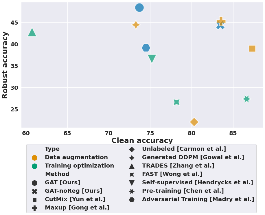
Figure 3: Comparison of GAT performances with state-of-the-art AT mechanisms on CIFAR-10 classification. In yellow AT with data augmentations and in green techniques with AT optimizations. GAT outperforms all existing approaches in terms of robust accuracy and remains competitive in terms of clean accuracy.

We show in Fig. 3 (and Appendix B.3) the clean and robust accuracy on CIFAR-10 of AT with various optimizations compared to AT with our approach. GAT outperforms data-augmentation AT techniques in terms of robust accuracy from 3.14% to 26.4% points, and outperforms AT training optimizations up to 21.82%.

GAT increases up to 41% the robustness of medical diagnosis.

Figure 4 shows the clean and robust AUC of the single-task baseline models (circle marker), and the task-augmented models.

For Atelectasis (blue), age task augmentation leads to lower results than the baseline. However, all remaining task augmentations outperform the baseline both on the clean and robust AUC. The gender augmentation increases the robust AUC of Atelectasis from 58.75% to 83.34%.

For Edema (orange), Task augmentation with Jigsaw leads to the best clean and robust AUC increase. The robust AUC jumps from 55.68% to 70.47% compared to single-task AT.

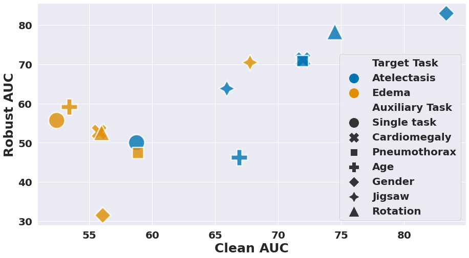
Figure 4: Comparison of different Task Augmentation strategies with single-task models using AT; Clean and robust AUC of GAT vs Single task AT of models trained to diagnose Atelectasis and Edema pathologies.

Table 1: The mean and std across three runs for combinations of our approach with data augmentation techniques. The blue cells indicate the combinations where GAT outperform data augmentation techniques with statistical significance, the underlined cells are the combinations that outperform task augmentation alone and, in bold the best performances.

Task	Robust accuracy (%)				Clean accuracy (%)
Augment	None	Jigsaw	Macro	Rotation	None	Jigsaw	Macro	Rotation
None	39.09$\pm$0.13	32.95$\pm$0.59	48.38$\pm$0.11	36.13$\pm$0.29	74.49$\pm$0.16	43.99$\pm$0.36	73.70$\pm$0.51	56.51$\pm$0.12
Cutmix	38.95$\pm$0.32	23.86$\pm$0.55	41.09$\pm$0.22	20.19$\pm$0.04	87.31$\pm$0.12	60.53$\pm$1.10	87.52$\pm$0.16	87.86$\pm$0.33
Unlabeled	21.98$\pm$0.18	26.33$\pm$0.28	33.88$\pm$0.15	35.29$\pm$0.20	80.30$\pm$0.41	49.32$\pm$1.06	84.57$\pm$0.05	71.08$\pm$0.08
Pre-train	27.30$\pm$0.40	35.47$\pm$0.38	32.64$\pm$0.27	33.78$\pm$0.35	86.64$\pm$0.26	87.56$\pm$0.18	86.69$\pm$0.31	87.85$\pm$0.21

GAT and data augmentation strategies can be combined to improve clean and robust performances.

The regularization term of the curvature measure used in GAT involves and may negatively impacts clean performance. We investigate if combining GAT with data-augmentation techniques can mitigate these effects. We show in Table 1 that GAT with various data augmentation strategies achieves higher robust accuracy than models with data augmentation alone in seven of the nine cases (in blue, Table 1). The two exceptions are CutMix when combined with Jigsaw or Rotation. Compared to GAT alone, all combinations of GAT with data augmentation show a slight drop in robustness (e.g., GAT with Rotation drops from 36.13% to 33.78%) but significantly improve clean accuracy. For example, they increase from 56.51% to 87.85% using the Rotation auxiliary task.

6 Ablation studies

We demonstrate in the following why the implementation choices of our approach GAT are the best, and how other choices impact the performance of GAT.

Impact of weighting strategies.

We proposed to formulate the AT process through the lens of Pareto-stationary optimization. We argue that this Pareto approach is more relevant than other multi-task strategies to handle adversarial and clean losses across multiple (potential) opposing tasks. To confirm this hypothesis, we provide in Table 2 an ablation study of GAT on the CIFAR-10 dataset. Both best clean and robust performances are achieved by GAT.

Moreover, GAT achieved best the pareto-optimum. We construct the front obtained by each weighting strategy, then compute its associated hyper-volume metric. This metric measures the volume of the dominated portion of the objective space and lower values indicate better pareto fronts. The best values are achieved by GAT with MGDA in Appendix C.3.

Table 2: Ablation study of the impact of the weighting strategies on the test and robust accuracies.

	Test acc	Robust acc
Macro Task + Equal weights	83.00 %	32.16 %
Macro Task + MGDA (Ours)	73.70 %	48.38 %
Macro Task + GV (Wang et al., 2020)	64.11 %	35.56 %
Macro Task + PCG (Yu et al., 2020)	63.76 %	44.74 %

Impact of task-dependent adversarial perturbations.

As our primary focus is the robustness of the main task only, we generate the perturbation $\delta$ only on the main task as presented in step 1 of Figure 2. Therefore, the perturbation $\delta$ is independent of the auxiliary tasks in Equation 5. One can also generate adversarial examples dependent on the auxiliary tasks. It can be relevant if we want to robustify all the tasks of the model together. This study differs from the threat model and objectives of our paper. Nevertheless, we evaluate in Table 3 the three cases.

Our findings indicate that there is no transferability from the Jigsaw task (the robustness improved from 0 to 1.64%), weak transferability from the Rotation task which improves the robustness to 12.22%), and strong transferability from the Macro task (where the robustness improved to 41.98%). We can explain this phenomenon by how related are the auxiliary tasks to the main task. Indeed, the Macro task is the most related to the main task. We acknowledge that further research is needed in this area, and we appreciate your interest in our work.

Overall, our results suggest that robustifying both tasks require additional optimizations. Indeed, it suggests that $\delta$ generated on both tasks does not robustify the main task for Jigsaw and Rotation, and can significantly deteriorate its clean performance.

Table 3: Comparison of GAT for models adversarially trained with a perturbation $\delta$ dependent of the main task only, or a perturbation $\delta$ dependant of both tasks.

AT on	Auxiliary task	Test acc	Robust acc
	None	74.49 %	39.09 %
Main only	Jigsaw	43.99 %	32.95 %
	Rotation	56.51 %	36.13 %
	Macro	73.70 %	48.38 %
Both tasks	Jigsaw	32.20 %	17.20 %
	Rotation	44.90 %	24.80 %
	Macro	75.20 %	36.50 %
Auxiliary only	Jigsaw	79.70 %	1.64%
	Rotation	86.03%	12.22%
	Macro	83.98%	41.98 %

Impact of the number of tasks

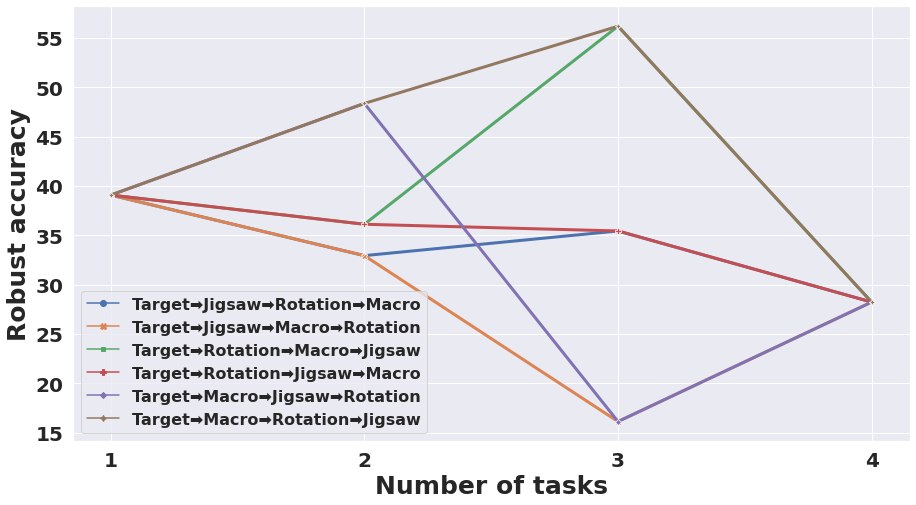
Figure 5: Adversarial robustness’ change when adding additional tasks then AT from scratch with GAT.

While our approach is proven for two tasks (because of Theorem 3 and MGDA), we hypothesize that it can still achieve higher robustness than SoTA with additional tasks. We show in Figure 5 how GAT behaves with additional tasks. Performances peak at three tasks using the combination of Macro and Rotation auxiliary tasks, while AT with combinations of three or four tasks involving the Jigsaw task remains less effective.

7 Generalization studies

Table 4: Robust accuracy of different models AT with GAT, with 3 different task augmentations, compared to their counterpart single task AT. In bold the cases where GAT outperforms single-task AT.

Scenario	Auxiliary task
	None	Jigsaw	Macro	Rotation
AutoAttack	27.01	29.63	32.54	13.82
AutoPGD	40.00	23.00	40.90	21.00
FAB	61.90	34.30	63.40	56.10
Transfer	1.53	13.44	10.8	15.45
WideResnet28	42.52	32.75	46.6	41.06

For a fair computational cost comparison, we compared GAT with AT techniques on the same Resnet50 architecture and training protocol. Some AT leverage larger models or datasets, or longer training to achieve better robustness on standardized benchmarks (Croce et al., 2020). We study in the following whether GAT can generalize to more complex datasets and tasks, larger models, or different threat models.

Generalization to dense tasks.

While our study focused on classification tasks, GAT can be deployed with self-supervised dense tasks like auto-encoders or depth estimation. To confirm the generalization of our approach, we evaluate an additional dataset: ROBIN; one of the most recent benchmarks to evaluate robustness of models (Zhao et al., 2021). We evaluate 3 additional self-supervised dense tasks: Depth estimation, Histogram of Oriented Gradients, and Auto-encoder. We evaluate these tasks both on CIFAR-10 and ROBIN. Our results in Table 5 suggest that dense tasks can also be used to improve the robustness of models.

Table 5: Comparison of the performance GAT for models adversarially trained with dense tasks.

Dataset	Auxiliary Task	Test acc	Robust acc
CIFAR10	No auxiliary	74.49 %	39.09 %
	Depth estimation	43.12 %	0.5 %
	HOG	83.39 %	44.59 %
	Auto-encoder	85.11 %	42.23 %
ROBIN	No auxiliary	93.71 %	56.78 %
	Depth estimation	87.43 %	18.54 %
	HOG	98.59 %	94.93 %
	Auto-encoder	98.78 %	94.84 %

Generalization to larger architectures.

We train WideResnet28-10 models with GAT and compare their robust accuracy to a single-task WideResnet28-10 model with AT. Macro increases the single-task model’s robust accuracy from 42.52% to 46.6%.

Generalization to adaptive attacks.

To assess if GAT is not a gradient-obfuscation defense, we evaluate our defended models against a large set of adversarial attacks. AutoPGD(Croce & Hein, 2020a), a parameter-free gradient attack, and FAB(Croce & Hein, 2020b), a white-box boundary attack. Autoattack (Croce & Hein, 2020c) is an ensemble that combines the previous white-box attacks with the black-box attack SquareAttack(Andriushchenko et al., 2020) in targeted and untargeted threat models.

The results in Table 4 show that GAT with Jigsaw or Macro auxiliary tasks provide better robustness to AutoAttack than AT with the target task alone. Thus, we confirm that stronger attacks do not easily overcome the robustness provided by GAT.

Generalization to transfer attacks.

We evaluate in Table 4 the threat model where the attacker has access to the full training set but has no knowledge of the auxiliary tasks leveraged by GAT. Models trained with GAT have slightly different decision boundaries from models with common AT. The success rate of surrogate attacks drops from 98.47% (i.e., 1.53% robust accuracy) to 84.55% when we train the target task with Rotation based GAT.

Generalization to extremely scarce data.

We restrict the AT of the models to 10% of the full CIFAR-10 training dataset and compare the performance of AT with GAT. GAT with self-supervised tasks and GAT with domain-knowledge tasks both outperform single-task model AT. In particular, the Macro task augmentation boosts the robust accuracy from 8.37% to 22.42%. The detailed results with 10%, 25%, and 50% of training data are in Appendix B.3.

8 Related Work

Multi-task learning

Vandenhende et al. (2021) recently proposed a new taxonomy of MTL approaches. They organized MTL research around two main questions: (i) which tasks should be learned together and (ii) how we can optimize the learning of multiple tasks. For example, there are multiple grouping and weighting strategies such as Gradient Vaccine (GV) (Wang et al., 2020), and Project Conflicting Gradients (PCG) (Yu et al., 2020) that can significantly impact the training of MT models.

Multi-objective optimization for large number of tasks remains also an open-problem, and the recent work from Standley et al. (2020b) investigated which tasks can be combined to improve clean performance.

Our work explores the orthogonal question of robustness: (iii) how can we combine auxiliary tasks with AT to improve the adversarial robustness?

Self-supervised multi-task learning

Recent work has evaluated the impact of self-supervised tasks on the robustness. Klingner et al.  (Klingner et al., 2020) evaluated how the robustness and performances are impacted by MTL for depth tasks. Their study does not tackle at all adversarial training and focuses on vanilla training. Hendrycks et al.  (Hendrycks et al., 2019) evaluated the robustness of multi-task models with rotation tasks to PGD attacks. However, they do not take into account the MTL in the adversarial process. PGD is applied summed on both the losses and is therefore used as a single task model.

Adversarial training

The original AT formulation has been improved, either to balance the trade-off between standard and robust accuracy like TRADES (Zhang et al., 2019) and FAT (Zhang et al., 2020), or to speed up the training (Shafahi et al., 2019; Wong et al., 2020). Finally, AT was combined with data augmentation techniques, either with unlabeled data (Carmon et al., 2019), self-supervised pre-training (Chen et al., 2020), or Mixup (Rebuffi et al., 2021).

These approaches, while very effective, entail a computation overhead that can be prohibitive for practical cases like medical imaging. Our work suggests that GAT is a parallel line of research and can be combined with these augmentations.

Provable robustness

This type of robustness is generally not comparable to empirical robustness (which we target) and is not considered in established robustness benchmarks like RobustBench(Croce et al., 2020). Provable robustness of MTL is therefore an orthogonal field to our research.

Conclusion

In this paper, we demonstrated that augmenting single-task models with self-supervised and domain-knowledge auxiliary tasks significantly improves the robust accuracy of classification. We proposed a novel adversarial training approach, Guided Adversarial Training that solves the min-max optimization of adversarial training through the prism of Pareto multi-objective learning and curvature regularization. Our approach complements existing data augmentation techniques for robust learning and improves adversarially trained models’ clean and robust accuracy. We expect that combining data augmentation and task augmentation is key for further breakthroughs in adversarial robustness.

Appendix A Appendix A: Replication

A.1 Proofs

Definition A.1.

Let $\mathscr{M}$ be a multi-task model. $\mathscr{T}^{\prime}\subseteq\mathscr{T}$ a subset of its tasks and $\mathcal{L}_{\mathscr{T}}^{\prime}$ the joint loss of tasks in $\mathscr{T}^{\prime}$. Then, we call $\mathbb{E}_{x}[\delta\mathcal{L}(\mathscr{T}^{\prime},\epsilon)]$ the adversarial vulnerability of $\mathscr{M}$ on $\mathscr{T}^{\prime}$ to an $\epsilon$-sized $\|.\|_{p}$-attack.

And we define it as the average increase of $\mathcal{L}_{\mathscr{T}^{\prime}}$ after attack over the whole dataset, i.e.:

$$\mathbb{E}_{x}[\delta\mathcal{L}(\mathscr{T}^{\prime},\epsilon)]=\mathbb{E}_{x}\left[\max_{\|\delta\|_{p}\leq\epsilon}\mid\mathcal{L}_{\mathscr{T}^{\prime}}(x+\delta,\bar{y})-\mathcal{L}_{\mathscr{T}^{\prime}}(x,\bar{y})\mid\right]$$

Lemma A.2.

Under an $\epsilon$-sized $\|.\|_{p}$-attack, the adversarial vulnerability of a multi-task model can be approximated through the first-order Taylor expansion, that is:

$$\mathbb{E}_{x}[\delta\mathcal{L}^{\prime}(x,\bar{y},\epsilon,\mathscr{T}^{\prime})]\propto\mathbb{E}_{x}[\mid\mid\partial_{x}\mathcal{L}^{\prime}(x,\bar{y})\mid\mid_{q}]$$ (6)

Proof.

From definition 1, we have:

$$\mathbb{E}_{x}[\delta\mathcal{L}(\mathscr{T}^{\prime},\epsilon)]=\mathbb{E}_{x}\left[\max_{\|\delta\|_{p}\leq\epsilon}\mid\mathcal{L}_{\mathscr{T}^{\prime}}(x+\delta,\bar{y})-\mathcal{L}_{\mathscr{T}^{\prime}}(x,\bar{y})\mid\right]$$

Given the perturbation $\delta$ is minimal, we can approximate $\delta\mathcal{L}$ with a Taylor expansion up to the first order:

$$\mathbb{E}_{x}[\delta\mathcal{L}(\mathscr{T}^{\prime},\epsilon)]=\mathbb{E}_{x}\left[\max_{\|\delta\|_{p}\leq\epsilon}\mid\mathcal{L}_{\mathscr{T}^{\prime}}(x+\delta,\bar{y})-\mathcal{L}_{\mathscr{T}^{\prime}}(x,\bar{y})\mid\right]\approx\mathbb{E}_{x}\left[\max_{\|\delta\|_{p}\leq\epsilon}\mid\delta\cdot\partial_{x}\mathcal{L}^{\prime}(x,\bar{y})\mid\right]$$

The noise $\delta$ is optimally adjusted to the coordinates of $\partial_{x}\mathcal{L}^{\prime}$ within an $\epsilon$-constraint. By the definition of the dual-norm, we get:

$$\mathbb{E}_{x}[\delta\mathcal{L}^{\prime}(x,\bar{y},\delta,\mathscr{T}^{\prime})]\approx\mid\mid\delta\mid\mid_{p}\cdot\mathbb{E}_{x}[\mid\mid\partial_{x}\mathcal{L}^{\prime}(x,\bar{y})\mid\mid_{q}]$$ (7)

where $q$ is the dual norm of $p$ and $\frac{1}{p}+\frac{1}{q}=1$ and $1\leq p\leq\infty$.

Once given the p-norm bounded ball, i.e., $\mid\mid\delta\mid\mid_{p}$ is constant (denoted $C$ in the following), we get:

$$\mathbb{E}_{x}[\delta\mathcal{L}^{\prime}(x,\bar{y},\epsilon,\mathscr{T}^{\prime})]\approx C\cdot\mathbb{E}_{x}[\mid\mid\partial_{x}\mathcal{L}^{\prime}(x,\bar{y})\mid\mid_{q}]\propto\mathbb{E}_{x}[\mid\mid\partial_{x}\mathcal{L}^{\prime}(x,\bar{y})\mid\mid_{q}]$$ (8)

∎

Theorem A.3.

Consider a multi-task model $\mathscr{M}$ where an attacker targets $\mathscr{T}=\{t_{1},t_{2}\}$ two tasks weighted with $\alpha_{1}$ and $\alpha_{2}$ respectively, with an $\epsilon$-sized $\|.\|_{p}$-attack. If the model is converged, and the gradient for each task is i.i.d. with zero mean and the tasks are correlated, the adversarial vulnerability of the model can be approximated as

$$\mathbb{E}_{x}[\delta\mathcal{L}^{\prime}]\propto\sqrt{1+2\frac{\alpha_{1}.\alpha_{2}.\operatorname{Cov}\left(\partial_{x}\mathcal{L}_{1},\partial_{x}\mathcal{L}_{2}\right)}{\alpha_{1}^{2}\sigma_{1}^{2}+\alpha_{2}^{2}\sigma_{2}^{2}}},$$ (9)

where $\sigma_{i}^{2}=\operatorname{Cov}\left(\partial_{x}\mathcal{L}_{i},\partial_{x}\mathcal{L}_{i}\right)$ and $\partial_{x}\mathcal{L}(x,y_{i})$ the gradient of the task $i$.

A.2

Proof.

let $\mathbf{r}_{i}=\alpha_{i}\cdot\partial_{x}\mathcal{L}(x,y_{i})$ the weighted gradient of the task i, with a weight $\alpha_{i}$ such as the joint gradient of $\mathscr{M}$ is defined as $\partial_{x}\mathcal{L}(x,\bar{y})=\sum_{i=1}^{M}\mathbf{r}_{i}$. let $p=q=2$

We have:

$$\mathbb{E}_{x}\left[\mid\mid C\cdot\partial_{x}\mathcal{L}^{\prime}(x,\bar{y})\mid\mid_{2}^{2}\right]=\mathbb{E}_{x}\left[\mid\mid\sum_{j=1}^{M}C\cdot r_{i}\mid\mid_{2}^{2}\right]$$ (10)

$$=C^{2}\mathbb{E}_{x}\left[\sum_{i=1}^{M}\mid\mid\mathbf{r}_{i}\mid\mid_{2}^{2}+2\sum_{i=1}^{M}\sum_{j=1}^{i-1}\mid\mid\mathbf{r}_{i}\mid\mid_{2}\mid\mid\mathbf{r}_{j}\mid\mid_{2}\right]$$

$$=C^{2}\left(\sum_{i=1}^{M}\mathbb{E}_{x}[\mathbf{r}_{i}^{2}]+2\sum_{i=1}^{M}\sum_{j=1}^{i-1}\mathbb{E}_{x}[\mathbf{r}_{i}\mathbf{r}_{j}]\right)$$

For two tasks, we have then:

$$\mathbb{E}_{x}\left[\mid\mid C\cdot\partial_{x}\mathcal{L}^{\prime}(x,\bar{y})\mid\mid_{2}^{2}\right]=C^{2}\left(\mathbb{E}_{x}[\mathbf{r}_{1}^{2}]+\mathbb{E}_{x}[\mathbf{r}_{2}^{2}]+2\mathbb{E}_{x}[\mathbf{r}_{1}\mathbf{r}_{2}]\right)$$ (11)

We know:

$$\operatorname{Cov}\left(\mathbf{r}_{i},\mathbf{r}_{j}\right)=\mathbb{E}_{x}\left[\mathbf{r}_{i}\mathbf{r}_{j}\right]-\mathbb{E}_{x}\left[\mathbf{r}_{i}\right]\mathbb{E}_{x}\left[\mathbf{r}_{j}\right]$$ (12)

According to the assumptions, the gradient of each task is i.i.d with zero means: $\mathbb{E}_{x}\left[\mathbf{r}_{i}\right]=0$ Then $\operatorname{Cov}\left(\mathbf{r}_{i},\mathbf{r}_{j}\right)=\mathbb{E}_{x}\left[\mathbf{r}_{i}\mathbf{r}_{j}\right]$ and $\mathbb{E}_{x}\left[\mathbf{r}_{i}^{2}\right]=\operatorname{Cov}\left(\mathbf{r}_{i},\mathbf{r}_{i}\right)=\alpha_{i}^{2}\operatorname{Cov}\left(\partial_{x}\mathcal{L}_{i},\partial_{x}\mathcal{L}_{i}\right)=\alpha_{i}^{2}\sigma_{i}^{2}$.

$$\mathbb{E}_{x}\left[\mid\mid C\cdot\partial_{x}\mathcal{L}^{\prime}(x,\bar{y})\mid\mid_{2}^{2}\right]={C^{2}}\left(\alpha_{1}^{2}\sigma_{1}^{2}+\alpha_{2}^{2}\sigma_{2}^{2}+2\cdot\alpha_{1}\alpha_{2}\operatorname{Cov}\left(\partial_{x}\mathcal{L}_{1},\partial_{x}\mathcal{L}_{2}\right)\right)$$ (13)

$$=K\cdot\left(1+2\frac{\alpha_{1}\alpha_{2}\operatorname{Cov}\left(\partial_{x}\mathcal{L}_{1},\partial_{x}\mathcal{L}_{2}\right)}{\alpha_{1}^{2}\sigma_{1}^{2}+\alpha_{2}^{2}\sigma_{2}^{2}}\right)$$

$$C\cdot\mathbb{E}_{x}\left[\mid\mid\partial_{x}\mathcal{L}^{\prime}(x,\bar{y})\mid\mid_{2}\right]=\sqrt{K}\cdot\sqrt{\left(1+2\frac{\alpha_{1}\alpha_{2}\operatorname{Cov}\left(\partial_{x}\mathcal{L}_{1},\partial_{x}\mathcal{L}_{2}\right)}{\alpha_{1}^{2}\sigma_{1}^{2}+\alpha_{2}^{2}\sigma_{2}^{2}}\right)}$$

where $K=C^{2}(\alpha_{1}^{2}\sigma_{1}^{2}+\alpha_{2}^{2}\sigma_{2}^{2})$

Using the first order adversarial vulnerability (Lemma 2), we then have:

$$\mathbb{E}_{x}[\delta\mathcal{L}^{\prime}]\approx C\cdot\mathbb{E}_{x}\left[\mid\mid\partial_{x}\mathcal{L}^{\prime}(x,\bar{y})\mid\mid_{2}\right]\approx\sqrt{K}\cdot\sqrt{1+2\frac{\alpha_{1}\alpha_{2}\operatorname{Cov}\left(\partial_{x}\mathcal{L}_{1},\partial_{x}\mathcal{L}_{2}\right)}{\alpha_{1}^{2}\sigma_{1}^{2}+\alpha_{2}^{2}\sigma_{2}^{2}}}\propto\sqrt{1+2\frac{\alpha_{1}.\alpha_{2}.\operatorname{Cov}\left(\partial_{x}\mathcal{L}_{1},\partial_{x}\mathcal{L}_{2}\right)}{\alpha_{1}^{2}\sigma_{1}^{2}+\alpha_{2}^{2}\sigma_{2}^{2}}}$$ (14)

with K a constant dependent of the bounded ball and the attacked tasks.

∎

A.3 GAT Algorithm

Algorithm 2 Pseudo-Algorithm of GAT

  Given: a single task model $\mathscr{M}$ parameterized by $\theta^{s}$ for the shared encoder and $\theta^{t}$ for the specific heads, a batch example $x$, and $\bar{y}=(y_{1},...,y_{s},...y_{m})$ its corresponding labels for each task, with $y_{1}$ the target task, $y_{1<i\leq s}$ the auxiliary self-supervised tasks and $y_{s<i\leq m}$ the auxiliary domain-knowledge tasks;

  Given: an input processing $f_{t}$ for each auxiliary self-supervised $t$ task with label $y_{1<t\leq s}$.

  Given: a weight optimizer $opt$; a list of task-specific decoders functions $\mathscr{D}=\{D_{1},...,D_{M}\}$

  Given: a $PGD$ adversarial attack with a step size $\epsilon_{step}$; a maximum perturbation $\epsilon$; $S$ number of attack iterations;

  Step 1: Create a decoder $D_{i}$ at the penultimate layer of $\mathscr{M}$ for each of the auxiliary task $t_{i}$ / $i>1$.

  Step 2: For each epoch and batch $x$ Do

1. For each self-supervised task $t_{1<i\leq s}$, successively pre-process the batch examples $x$ with the appropriate input processing function:
   $x\leftarrow\operatorname*{\bigcirc}_{t=2}^{s}\ f_{t}(x)$

2. Generate $\hat{x}$, the adversarial examples of $x$: $\hat{x}\leftarrow\mathrm{PGD}(x,y_{1},\epsilon_{step},\epsilon,S)$.

3. Compute the losses $l_{i,x}$ and $l_{i,\hat{x}}$ of $x$ and $\hat{x}$ respectively for each task $t_{i}$ with label $y_{i}$; $l\leftarrow l_{1,x},l_{1,\hat{x}},\ldots,l_{M,x},l_{M,\hat{x}},l^{(reg)}_{M+1,x},\ldots,l^{(reg)}_{2M-1,x}$.

4. Apply MGDA to find the minimum norm element in the convex hull given the list of losses:
   $\alpha_{1},\ldots,\alpha_{2M-1}\leftarrow$ MGDA($\theta^{s},\theta^{t}\theta$,$l$)

5. Back-propagate the weighted gradients and update the model weights with optimizer $opt$.
   $\theta^{s}\leftarrow\theta^{s}-\eta\sum_{t=1}^{2M-1}\alpha_{t}\nabla_{\theta^{sh}}l_{t,x}(\theta^{s},\theta^{t})$

  Step 3: Disable the auxiliary branches added at step 1.

Following Sener & Koltun (2018), we use the Frank-Wolfe algorithm(Jaggi, 2013) to solve the constrained optimization problem as follows:

Algorithm 3 MGDA($\theta^{s},\theta^{t}$,$l$) procedure (Sener & Koltun, 2018)

  Initialize $\alpha=(\alpha^{1},\ldots,\alpha^{T})=(\frac{1}{T},\ldots,\frac{1}{T})$

  Precompute $\mathcal{M}$ st. $\mathcal{M}_{i,j}=\big{(}\nabla_{\theta^{sh}}\hat{l}_{i}(\theta^{sh},\theta^{i})\big{)}^{\intercal}\big{(}\nabla_{\theta^{sh}}\hat{l}_{j}(\theta^{sh},\theta^{j})\big{)}$

  Repeat

   $\hat{t}=\operatorname*{arg\,min}_{r}\sum_{t}\alpha^{t}\mathcal{M}_{rt}$

   $\hat{\gamma}=\operatorname*{arg\,min}_{\gamma}\big{(}(1-\gamma)\bm{\alpha}+\gamma\bm{e}_{\hat{t}}\big{)}^{\intercal}\mathcal{M}\big{(}(1-\gamma)\bm{\alpha}+\gamma\bm{e}_{\hat{t}}\big{)}$

  $\bm{\alpha}=(1-\hat{\gamma})\bm{\alpha}+\hat{\gamma}\bm{e}_{\hat{t}}$

  until $\hat{\gamma}\sim 0$ or Number of Iterations Limit

  return $\alpha^{1},\ldots,\alpha^{T}$

A.4 Experimental Setting

A.4.1 Datasets

We show in table 6 the general properties of the datasets used in training our models. Table 7 ((Cohen et al., 2020)) details the number of positive and negative examples with each label for each dataset. Our models are trained either on CheXpert or NIH depending on the evaluation.

Our evaluation covers as target tasks very scarce pathologies (Edema, Pneumonia), and medium scarce pathologies (Atelectasis), across both datasets.

	NIH	CheXpert
Number of patient radiographs	112,120	224,316
Number of patients	30,805	65,240
Age in years: mean (standard deviation)	46.9 (16.6)	60.7 (18.4)
Percentage of females (%)	43.5%	40.6%
Number of pathology labels	8	14

Table 6: Characteristics of NIH and CheXpert datasets used in our evaluation.

Dataset	NIH	CheXpert
Atelectasis	1702/29103	12691/14317
Cardiomegaly	767/30038	9099/17765
Consolidation	427/30378	5390/22504
Edema	82/30723	14929/20615
Effusion	1280/29525	20640/23500
Emphysema	265/30540	-
Enlarged Cardio	-	5181/20506
Fibrosis	571/30234	-
Fracture	-	4250/14948
Hernia	83/30722	-
Infiltration	3604/27201	-
Lung Lesion	-	4217/14422
Lung Opacity	-	30873/15675
Mass	1280/29525	-
Nodule	1661/29144	-
Pleural Thickening	763/30042	-
Pneumonia	168/30637	2822/14793
Pneumothorax	269/30536	4311/32685

Table 7: Samples distributions across each pathology and dataset. Each cell shows the number of positive/negative samples of the label. There are 7 common pathologies in NIH and CheXpert datasets. Among those, in bold the pathologies evaluated as target task, and in underline the pathologies used as an auxiliary.

All datasets, CheXpert, NIH, and ROBIN use images of the same dimensions as ImageNet (256x256). We did not include Tiny ImageNet in our study as it lacks multiple tasks required for a comprehensive evaluation. Furthermore, we chose the ROBIN dataset as it is a subset of ImageNet that offers additional labels that can serve as auxiliary task, making it the most suitable variant for our study.

A.5 Architectures

The majority of the tests are carried out using the Resnet50v2 (He et al., 2016) encoder, which has a depth of 50 and 25.6M parameters. This encoder is the main focus because it is the most widely used for Xray image classification (Ganesan et al., 2019). We also perform some tests using the WRN-28-10 (Zagoruyko & Komodakis, 2016) encoder, which has a depth of 28, a width multiplier of 10, and 36M parameters.

A.6 Adversarial Training

The outer minimization:

We use MADRY adversarial training (Madry et al., 2017a), i.e. we train the model using a summed loss computed from the clean and adversarial examples. for ATTA, we use a backpropagation over the pareto optimal of the four losses. The learning uses the SGD optimizer with lr=0.1, a cosine annealing, and checkpoint over the best performance.

The inner maximization:

We generate the adversarial examples with PGD (Madry et al., 2017b), on $\ell_{\infty}$ norms and $\epsilon=8/255$ for CIFAR-10 and STL-10 and $\epsilon=4/255$ for CheXpert and NIH models. We use in the iterative attack 1 random start, and 10 steps.

A.7 Robustness evaluation

We evaluate the robustness against PGD-10 on $\ell_{\infty}$ norms and $\epsilon=8/255$ for CIFAR-10 and STL-10 and $\epsilon=4/255$ for CheXpert and NIH models. We also evaluate CIFAR-10 models against AutoAttack (Croce & Hein, 2020a). Autoattack is a mixture of $\ell_{\infty}epsilon=8/255$ attacks: untargeted AUTOPGD (a variant of PGD with an adaptive step) on the cross-entropy loss with 100 steps, targeted AUTOPGD with 100 steps, a 100 steps FAB attack, and finally a 5000 queries Square attack.

These hyper-parameters of AutoAttack are consistent with AutoAttack’s default parameterization in Kim (2020); Croce et al. (2020).

A.8 Computation budget

We train all our models on slurm nodes, using single node training. Each node has one A100 GPU 32Gb V100 SXM2. We train CIFAR-10 and STL-10 models for 400 epochs and CheXpert and NIH models for 200 epochs. The WRN-70-16 model is trained for 40 epochs to account for being 10 times larger than the Resnet50 used for the main evaluation.

Our license is MIT Licence, and we use the following external packages:

Torchxrayvision:

Located in folder ./torchxrayvision. Adapted from https://github.com/mlmed/torchxrayvision: Apache Licence

Taskonomy/Taskgrouping:

Located in folder ./utils/multitask_models. Adapted from https://github.com/tstandley/taskgrouping/ MIT Licence

LibMTL:

Located in folder ./utils/weights. Adapted from https://github.com/median-research-group/LibMTL MIT Licence

Appendix B Appendix B: Detailed results of the main study

B.1 Limited data training with CIFAR-10

GAT:

To evaluate whether test accuracy (i.e. equal weights task augmentation) is effective when access to adversarial training data is limited, we first train models with the full dataset for 200 epochs then we adversarial fine-tune (PGD-4; 8/255) the models with a subset of training data (10%, 50%). For each scenario, we fine-tune 3 different models with different seeds and report in Table 8 the Test Accuracy (Test accuracy) and Robust Accuracy (Robust accuracy) with and without an auxiliary task. We report the mean and standard deviation across the runs. The std across the experiments is pretty low and the conclusions of the main paper hold.

Table 8: Evaluation results of 4 Different ($\mathcal{D}_{i},\mathcal{T}_{i},\mathcal{A}_{i}$) Scenarios: $\mathcal{D}_{1}$ (adversarial fine-tuning with 10% of the training data), $\mathcal{D}_{2}$ (adversarial fine-tuning with 50% of the training data), $\mathcal{T}_{1,2,3}$ training respectively without an auxiliary task, with Rotation and with Jigsaw task, $\mathcal{A}_{1}$ (Robust Accuracy against a PGD-4 attack), $\mathcal{A}_{2}$ (Robust Accuracy against a PGD-10 attack).

Dataset subset	Auxiliary	PGD steps	Metric	mean	std
0.1	None	10	Test accuracy	60.41	0.62
			Robust accuracy	8.37	0.32
		4	Test accuracy	60.38	0.59
			Robust accuracy	11.81	0.23
	Jigsaw	10	Test accuracy	51.98	0.53
			Robust accuracy	32.41	0.46
		4	Test accuracy	51.06	1.47
			Robust accuracy	32.26	0.85
	Rotation	10	Test accuracy	50.41	0.11
			Robust accuracy	15.01	0.29
		4	Test accuracy	50.17	0.49
			Robust accuracy	20.01	0.27
	Macro	10	Test accuracy	65.62	0.48
			Robust accuracy	22.42	0.35
		4	Test accuracy	65.65	0.42
			Robust accuracy	42.68	0.38
0.5	None	10	Test accuracy	77.45	0.25
			Robust accuracy	25.04	0.15
		4	Test accuracy	77.51	0.15
			Robust accuracy	31.71	0.08
	Jigsaw	10	Test accuracy	59.72	0.45
			Robust accuracy	29.08	1.58
		4	Test accuracy	58.42	1.16
			Robust accuracy	33.68	0.52
	Rotation	10	Test accuracy	59.77	0.58
			Robust accuracy	17.09	0.51
		4	Test accuracy	59.69	0.70
			Robust accuracy	24.56	0.49
	Macro	10	Test accuracy	73.68	0.72
			Robust accuracy	33.76	0.71
		4	Test accuracy	73.62	0.81
			Robust accuracy	54.14	0.63

B.2 CheXpert detailed results

We extend the evaluation of the main paper to 6 additional combinations of auxiliary tasks and target task, using the Pneumonia pathology as a target. We present all the results in Table 10. These extended results corroborate that AT with auxiliary task significantly improves the robustness of classification models on the CheXpert dataset (Irvin et al., 2019).

Table 9: GAT different data scenarios: 10%, 25% and 50% of CIFAR-10 dataset. We evaluate 3 different task augmentations with MGDA weighting strategy.

Scenario	Clean accuracy (%)				Robust accuracy (%)
	None	Jigsaw	Macro	Rotation	None	Jigsaw	Macro	Rotation
10%	52.66	42.7	54.89	47.07	12.46	32.14	13.43	39.2
25%	68.39	49.76	68.54	62.85	24.56	32.08	27.74	47.75
50%	76.13	66.57	76.5	78.19	33.69	23.79	31.94	16.63

Table 10: Robust and clean AUC of CheXpert models trained with GAT.

Target Task	Auxiliary Task	Robust AUC	Clean AUC
Atelectasis	Single task	50.00	58.76
Atelectasis	Cardiomegaly	71.20	71.97
Atelectasis	Pneumothorax	70.93	71.92
Atelectasis	Age	46.26	66.89
Atelectasis	Gender	83.00	83.35
Atelectasis	Jigsaw	63.81	65.92
Atelectasis	Rotation	78.32	74.50
Edema	Single task	55.69	52.42
Edema	Cardiomegaly	52.74	55.79
Edema	Pneumothorax	47.40	58.86
Edema	Age	59.17	53.41
Edema	Gender	31.46	56.07
Edema	Jigsaw	70.47	67.77
Edema	Rotation	52.59	55.98
Pneumonia	Single task	38.70	56.66
Pneumonia	Cardiomegaly	57.47	57.05
Pneumonia	Pneumothorax	32.25	56.74
Pneumonia	Age	49.15	56.58
Pneumonia	Gender	60.08	57.59
Pneumonia	Jigsaw	46.45	56.47
Pneumonia	Rotation	60.76	60.00

B.3 CIFAR10 detailed results

Table 11: Robust and clean Accuracy of CIFAR-10 models trained with GAT vs trained with other adversarial training (AT) optimizations

Method	Robust accuracy (%)	Clean accuracy (%)	Type of AT optimization
GAT [Ours]	48.38	73.70	Task augmentation
GAT-noReg [Ours]	44.34	83.47	Task augmentation
CutMix (Yun et al., 2019)	38.95	87.31	Data augmentation
Maxup (Gong et al., 2020)	45.24	83.54	Data augmentation
Unlabeled (Carmon et al., 2019)	21.98	80.30	Data augmentation
DDPM (Gowal et al., 2021)	44.41	73.27	Data augmentation
TRADES (Zhang et al., 2019)	42.76	60.73	Training optimization
FAST (Wong et al., 2020)	26.56	78.18	Training optimization
Self-supervised (Hendrycks et al., 2019)	36.50	75.20	Training & data optimization
Pre-training (Chen et al., 2020)	27.30	86.64	Training & data optimization
Madry Adversarial Training (Madry et al., 2017b)	39.09	74.49	Training optimization

We gather the performance of all SoTA adversarial training approaches in Table 11. GAT without regularization term has a lower robustness but preserves better the clean performance. For DDPM, we follow Gowal et al. (2021) and use samples generated by a Denoising Diffusion Probabilistic Model (Ho et al., 2020) to improve robustness. The DDPM is solely trained on the original training data and does not use additional external data. We do not however use the additional optimizations proposed by Gowal et al. (2021) to achieve their results, and stick to the same training protocol as all our experiments.

Their additional training optimizations are detailed in their repository: https://github.com/deepmind/deepmind-research/tree/master/adversarial_robustness/pytorch.

Appendix C Appendix C: Complementary results

C.1 Statistical significance when compared with SoTA

Dietterich suggests the McNemar’s test in seminal study on the use of statistical hypothesis tests to compare classifiers(Dietterich, 1998).

The test is particularly suggested when the methods being compared can only be assessed once, e.g. on a single test set, as opposed to numerous evaluations using a resampling methodology, such as k-fold cross-validation. It is also recommended when the computation cost of training the same model multiple times is high. Both are our cases in this study.

The results in Table 2 of the main paper use this statistical test. The blue cells are the ones where we can reject Null Hypothesis: Classifiers with ATTA vs without have a different proportion of errors on the test set. In our study, we use $\alpha=0.05$ and provide in the figshare repository https://figshare.com/projects/ATTA/139864 the Contingency tables and raw values of the test: You can find the sumary of the evaluation below:

• Model ’Rotation’ VS ’Macro’

  statistic=792.000, p-value=0.000

  Different proportions of errors (reject H0): The two classifiers have a different proportion of errors on the test

• Model ’Rotation’ VS ’Jigsaw’

  statistic=610.000, p-value=0.000

  reject H0

• Model ’Rotation’ VS ’Depth’

  statistic=464.000, p-value=0.000

  reject H0

• Model ’Rotation’ VS ’Hog’

  statistic=770.000, p-value=0.000

  reject H0

• Model ’Rotation’ VS ’Rot + Unlabeled’

  statistic=395.000, p-value=0.000

  reject H0

• Model ’Rotation’ VS ’Macro + Unlabeled’

  statistic=380.000, p-value=0.000

  reject H0

• Model ’Rotation’ VS ’Unlabeled’

  statistic=788.000, p-value=0.000

  reject H0

• Model ’Rotation’ VS ’Jigsaw + Unlabeled’

  statistic=638.000, p-value=0.000

  reject H0

• Model ’Rotation’ VS ’Rot + Cutmix’

  statistic=610.000, p-value=0.000

  reject H0

• Model ’Rotation’ VS ’Macro + Cutmix’

  statistic=842.000, p-value=0.010

  reject H0

• Model ’Rotation’ VS ’Jigsaw + Cutmix’

  statistic=590.000, p-value=0.000

  reject H0

• Model ’Macro’ VS ’Rotation’

  statistic=792.000, p-value=0.000

  reject H0

• Model ’Macro’ VS ’Jigsaw’

  statistic=502.000, p-value=0.000

  reject H0

• Model ’Macro’ VS ’Depth’

  statistic=372.000, p-value=0.000

  reject H0

• Model ’Macro’ VS ’Hog’

  statistic=460.000, p-value=0.095

  Same proportions of errors (fail to reject H0)

• Model ’Macro’ VS ’Rot + Unlabeled’

  statistic=509.000, p-value=0.000

  reject H0

• Model ’Macro’ VS ’Macro + Unlabeled’

  statistic=287.000, p-value=0.000

  reject H0

• Model ’Macro’ VS ’Unlabeled’

  statistic=715.000, p-value=0.103

  Same proportions of errors (fail to reject H0)

• Model ’Macro’ VS ’Jigsaw + Unlabeled’

  statistic=472.000, p-value=0.000

  reject H0

• Model ’Macro’ VS ’Rot + Cutmix’

  statistic=621.000, p-value=0.000

  reject H0

• Model ’Macro’ VS ’Macro + Cutmix’

  statistic=631.000, p-value=0.010

  reject H0

• Model ’Macro’ VS ’Jigsaw + Cutmix’

  statistic=468.000, p-value=0.000

  reject H0

• Model ’Jigsaw’ VS ’Rotation’

  statistic=610.000, p-value=0.000

  reject H0

• Model ’Jigsaw’ VS ’Macro’

  statistic=502.000, p-value=0.000

  reject H0

• Model ’Jigsaw’ VS ’Depth’

  statistic=1066.000, p-value=0.000

  reject H0

• Model ’Jigsaw’ VS ’Hog’

  statistic=523.000, p-value=0.000

  reject H0

• Model ’Jigsaw’ VS ’Rot + Unlabeled’

  statistic=344.000, p-value=0.000

  reject H0

• Model ’Jigsaw’ VS ’Macro + Unlabeled’

  statistic=255.000, p-value=0.000

  reject H0

• Model ’Jigsaw’ VS ’Unlabeled’

  statistic=563.000, p-value=0.000

  reject H0

• Model ’Jigsaw’ VS ’Jigsaw + Unlabeled’

  statistic=1116.000, p-value=0.000

  reject H0

• Model ’Jigsaw’ VS ’Rot + Cutmix’

  statistic=1415.000, p-value=0.000

  reject H0

• Model ’Jigsaw’ VS ’Macro + Cutmix’

  statistic=580.000, p-value=0.000

  reject H0

• Model ’Jigsaw’ VS ’Jigsaw + Cutmix’

  statistic=1278.000, p-value=0.444

  Same proportions of errors (fail to reject H0)

• Model ’Depth’ VS ’Rotation’

  statistic=464.000, p-value=0.000

  reject H0

• Model ’Depth’ VS ’Macro’

  statistic=372.000, p-value=0.000

  reject H0

• Model ’Depth’ VS ’Jigsaw’

  statistic=1066.000, p-value=0.000

  reject H0

• Model ’Depth’ VS ’Hog’

  statistic=390.000, p-value=0.000

  reject H0

• Model ’Depth’ VS ’Rot + Unlabeled’

  statistic=265.000, p-value=0.000

  reject H0

• Model ’Depth’ VS ’Macro + Unlabeled’

  statistic=192.000, p-value=0.000

  reject H0

• Model ’Depth’ VS ’Unlabeled’

  statistic=453.000, p-value=0.000

  reject H0

• Model ’Depth’ VS ’Jigsaw + Unlabeled’

  statistic=1218.000, p-value=0.000

  reject H0

• Model ’Depth’ VS ’Rot + Cutmix’

  statistic=816.000, p-value=0.000

  reject H0

• Model ’Depth’ VS ’Macro + Cutmix’

  statistic=352.000, p-value=0.000

  reject H0

• Model ’Depth’ VS ’Jigsaw + Cutmix’

  statistic=857.000, p-value=0.000

  reject H0

• Model ’Hog’ VS ’Rotation’

  statistic=770.000, p-value=0.000

  reject H0

• Model ’Hog’ VS ’Macro’

  statistic=460.000, p-value=0.095

  Same proportions of errors (fail to reject H0)

• Model ’Hog’ VS ’Jigsaw’

  statistic=523.000, p-value=0.000

  reject H0

• Model ’Hog’ VS ’Depth’

  statistic=390.000, p-value=0.000

  reject H0

• Model ’Hog’ VS ’Rot + Unlabeled’

  statistic=560.000, p-value=0.000

  reject H0

• Model ’Hog’ VS ’Macro + Unlabeled’

  statistic=312.000, p-value=0.000

  reject H0

• Model ’Hog’ VS ’Unlabeled’

  statistic=774.000, p-value=0.800

  Same proportions of errors (fail to reject H0)

• Model ’Hog’ VS ’Jigsaw + Unlabeled’

  statistic=484.000, p-value=0.000

  reject H0

• Model ’Hog’ VS ’Rot + Cutmix’

  statistic=629.000, p-value=0.000

  reject H0

• Model ’Hog’ VS ’Macro + Cutmix’

  statistic=631.000, p-value=0.000

  reject H0

• Model ’Hog’ VS ’Jigsaw + Cutmix’

  statistic=445.000, p-value=0.000

  reject H0

• Model ’Rot + Unlabeled’ VS ’Rotation’

  statistic=395.000, p-value=0.000

  reject H0

• Model ’Rot + Unlabeled’ VS ’Macro’

  statistic=509.000, p-value=0.000

  reject H0

• Model ’Rot + Unlabeled’ VS ’Jigsaw’

  statistic=344.000, p-value=0.000

  reject H0

• Model ’Rot + Unlabeled’ VS ’Depth’

  statistic=265.000, p-value=0.000

  reject H0

• Model ’Rot + Unlabeled’ VS ’Hog’

  statistic=560.000, p-value=0.000

  reject H0

• Model ’Rot + Unlabeled’ VS ’Macro + Unlabeled’

  statistic=470.000, p-value=0.000

  reject H0

• Model ’Rot + Unlabeled’ VS ’Unlabeled’

  statistic=475.000, p-value=0.000

  reject H0

• Model ’Rot + Unlabeled’ VS ’Jigsaw + Unlabeled’

  statistic=310.000, p-value=0.000

  reject H0

• Model ’Rot + Unlabeled’ VS ’Rot + Cutmix’

  statistic=261.000, p-value=0.000

  reject H0

• Model ’Rot + Unlabeled’ VS ’Macro + Cutmix’

  statistic=460.000, p-value=0.000

  reject H0

• Model ’Rot + Unlabeled’ VS ’Jigsaw + Cutmix’

  statistic=326.000, p-value=0.000

  reject H0

• Model ’Macro + Unlabeled’ VS ’Rotation’

  statistic=380.000, p-value=0.000

  reject H0

• Model ’Macro + Unlabeled’ VS ’Macro’

  statistic=287.000, p-value=0.000

  reject H0

• Model ’Macro + Unlabeled’ VS ’Jigsaw’

  statistic=255.000, p-value=0.000

  reject H0

• Model ’Macro + Unlabeled’ VS ’Depth’

  statistic=192.000, p-value=0.000

  reject H0

• Model ’Macro + Unlabeled’ VS ’Hog’

  statistic=312.000, p-value=0.000

  reject H0

• Model ’Macro + Unlabeled’ VS ’Rot + Unlabeled’

  statistic=470.000, p-value=0.000

  reject H0

• Model ’Macro + Unlabeled’ VS ’Unlabeled’

  statistic=225.000, p-value=0.000

  reject H0

• Model ’Macro + Unlabeled’ VS ’Jigsaw + Unlabeled’

  statistic=191.000, p-value=0.000

  reject H0

• Model ’Macro + Unlabeled’ VS ’Rot + Cutmix’

  statistic=292.000, p-value=0.000

  reject H0

• Model ’Macro + Unlabeled’ VS ’Macro + Cutmix’

  statistic=213.000, p-value=0.000

  reject H0

• Model ’Macro + Unlabeled’ VS ’Jigsaw + Cutmix’

  statistic=201.000, p-value=0.000

  reject H0

• Model ’Unlabeled’ VS ’Rotation’

  statistic=788.000, p-value=0.000

  reject H0

• Model ’Unlabeled’ VS ’Macro’

  statistic=715.000, p-value=0.103

  Same proportions of errors (fail to reject H0)

• Model ’Unlabeled’ VS ’Jigsaw’

  statistic=563.000, p-value=0.000

  reject H0

• Model ’Unlabeled’ VS ’Depth’

  statistic=453.000, p-value=0.000

  reject H0

• Model ’Unlabeled’ VS ’Hog’

  statistic=774.000, p-value=0.800

  Same proportions of errors (fail to reject H0)

• Model ’Unlabeled’ VS ’Rot + Unlabeled’

  statistic=475.000, p-value=0.000

  reject H0

• Model ’Unlabeled’ VS ’Macro + Unlabeled’

  statistic=225.000, p-value=0.000

  reject H0

• Model ’Unlabeled’ VS ’Jigsaw + Unlabeled’

  statistic=452.000, p-value=0.000

  reject H0

• Model ’Unlabeled’ VS ’Rot + Cutmix’

  statistic=574.000, p-value=0.000

  reject H0

• Model ’Unlabeled’ VS ’Macro + Cutmix’

  statistic=622.000, p-value=0.000

  reject H0

• Model ’Unlabeled’ VS ’Jigsaw + Cutmix’

  statistic=482.000, p-value=0.000

  reject H0

• Model ’Jigsaw + Unlabeled’ VS ’Rotation’

  statistic=638.000, p-value=0.000

  reject H0

• Model ’Jigsaw + Unlabeled’ VS ’Macro’

  statistic=472.000, p-value=0.000

  reject H0

• Model ’Jigsaw + Unlabeled’ VS ’Jigsaw’

  statistic=1116.000, p-value=0.000

  reject H0

• Model ’Jigsaw + Unlabeled’ VS ’Depth’

  statistic=1218.000, p-value=0.000

  reject H0

• Model ’Jigsaw + Unlabeled’ VS ’Hog’

  statistic=484.000, p-value=0.000

  reject H0

• Model ’Jigsaw + Unlabeled’ VS ’Rot + Unlabeled’

  statistic=310.000, p-value=0.000

  reject H0

• Model ’Jigsaw + Unlabeled’ VS ’Macro + Unlabeled’

  statistic=191.000, p-value=0.000

  reject H0

• Model ’Jigsaw + Unlabeled’ VS ’Unlabeled’

  statistic=452.000, p-value=0.000

  reject H0

• Model ’Jigsaw + Unlabeled’ VS ’Rot + Cutmix’

  statistic=1305.000, p-value=0.000

  reject H0

• Model ’Jigsaw + Unlabeled’ VS ’Macro + Cutmix’

  statistic=463.000, p-value=0.000

  reject H0

• Model ’Jigsaw + Unlabeled’ VS ’Jigsaw + Cutmix’

  statistic=968.000, p-value=0.000

  reject H0

• Model ’Rot + Cutmix’ VS ’Rotation’

  statistic=610.000, p-value=0.000

  reject H0

• Model ’Rot + Cutmix’ VS ’Macro’

  statistic=621.000, p-value=0.000

  reject H0

• Model ’Rot + Cutmix’ VS ’Jigsaw’

  statistic=1415.000, p-value=0.000

  reject H0

• Model ’Rot + Cutmix’ VS ’Depth’

  statistic=816.000, p-value=0.000

  reject H0

• Model ’Rot + Cutmix’ VS ’Hog’

  statistic=629.000, p-value=0.000

  reject H0

• Model ’Rot + Cutmix’ VS ’Rot + Unlabeled’

  statistic=261.000, p-value=0.000

  reject H0

• Model ’Rot + Cutmix’ VS ’Macro + Unlabeled’

  statistic=292.000, p-value=0.000

  reject H0

• Model ’Rot + Cutmix’ VS ’Unlabeled’

  statistic=574.000, p-value=0.000

  reject H0

• Model ’Rot + Cutmix’ VS ’Jigsaw + Unlabeled’

  statistic=1305.000, p-value=0.000

  reject H0

• Model ’Rot + Cutmix’ VS ’Macro + Cutmix’

  statistic=561.000, p-value=0.000

  reject H0

• Model ’Rot + Cutmix’ VS ’Jigsaw + Cutmix’

  statistic=1275.000, p-value=0.000

  reject H0

• Model ’Macro + Cutmix’ VS ’Rotation’

  statistic=842.000, p-value=0.010

  reject H0

• Model ’Macro + Cutmix’ VS ’Macro’

  statistic=631.000, p-value=0.010

  reject H0

• Model ’Macro + Cutmix’ VS ’Jigsaw’

  statistic=580.000, p-value=0.000

  reject H0

• Model ’Macro + Cutmix’ VS ’Depth’

  statistic=352.000, p-value=0.000

  reject H0

• Model ’Macro + Cutmix’ VS ’Hog’

  statistic=631.000, p-value=0.000

  reject H0

• Model ’Macro + Cutmix’ VS ’Rot + Unlabeled’

  statistic=460.000, p-value=0.000

  reject H0

• Model ’Macro + Cutmix’ VS ’Macro + Unlabeled’

  statistic=213.000, p-value=0.000

  reject H0

• Model ’Macro + Cutmix’ VS ’Unlabeled’

  statistic=622.000, p-value=0.000

  reject H0

• Model ’Macro + Cutmix’ VS ’Jigsaw + Unlabeled’

  statistic=463.000, p-value=0.000

  reject H0

• Model ’Macro + Cutmix’ VS ’Rot + Cutmix’

  statistic=561.000, p-value=0.000

  reject H0

• Model ’Macro + Cutmix’ VS ’Jigsaw + Cutmix’

  statistic=327.000, p-value=0.000

  reject H0

• Model ’Jigsaw + Cutmix’ VS ’Rotation’

  statistic=590.000, p-value=0.000

  reject H0

• Model ’Jigsaw + Cutmix’ VS ’Macro’

  statistic=468.000, p-value=0.000

  reject H0

• Model ’Jigsaw + Cutmix’ VS ’Jigsaw’

  statistic=1278.000, p-value=0.444

  Same proportions of errors (fail to reject H0)

• Model ’Jigsaw + Cutmix’ VS ’Depth’

  statistic=857.000, p-value=0.000

  reject H0

• Model ’Jigsaw + Cutmix’ VS ’Hog’

  statistic=445.000, p-value=0.000

  reject H0

• Model ’Jigsaw + Cutmix’ VS ’Rot + Unlabeled’

  statistic=326.000, p-value=0.000

  reject H0

• Model ’Jigsaw + Cutmix’ VS ’Macro + Unlabeled’

  statistic=201.000, p-value=0.000

  reject H0

• Model ’Jigsaw + Cutmix’ VS ’Unlabeled’

  statistic=482.000, p-value=0.000

  reject H0

• Model ’Jigsaw + Cutmix’ VS ’Jigsaw + Unlabeled’

  statistic=968.000, p-value=0.000

  reject H0

• Model ’Jigsaw + Cutmix’ VS ’Rot + Cutmix’

  statistic=1275.000, p-value=0.000

  reject H0

• Model ’Jigsaw + Cutmix’ VS ’Macro + Cutmix’

  statistic=327.000, p-value=0.000

  reject H0

The test is particularly suggested when the methods being compared can only be assessed once, e.g. on a single test set, as opposed to numerous evaluations using a resampling methodology, such as k-fold cross-validation.

C.2 GAT on a supplementary Chest X-ray dataset: NIH

We present in Figure 6 similar study of the main paper, but on the NIH dataset. Our conclusions that GAT outperforms Adversarial training (circles in 6) are confirmed on this dataset as well.

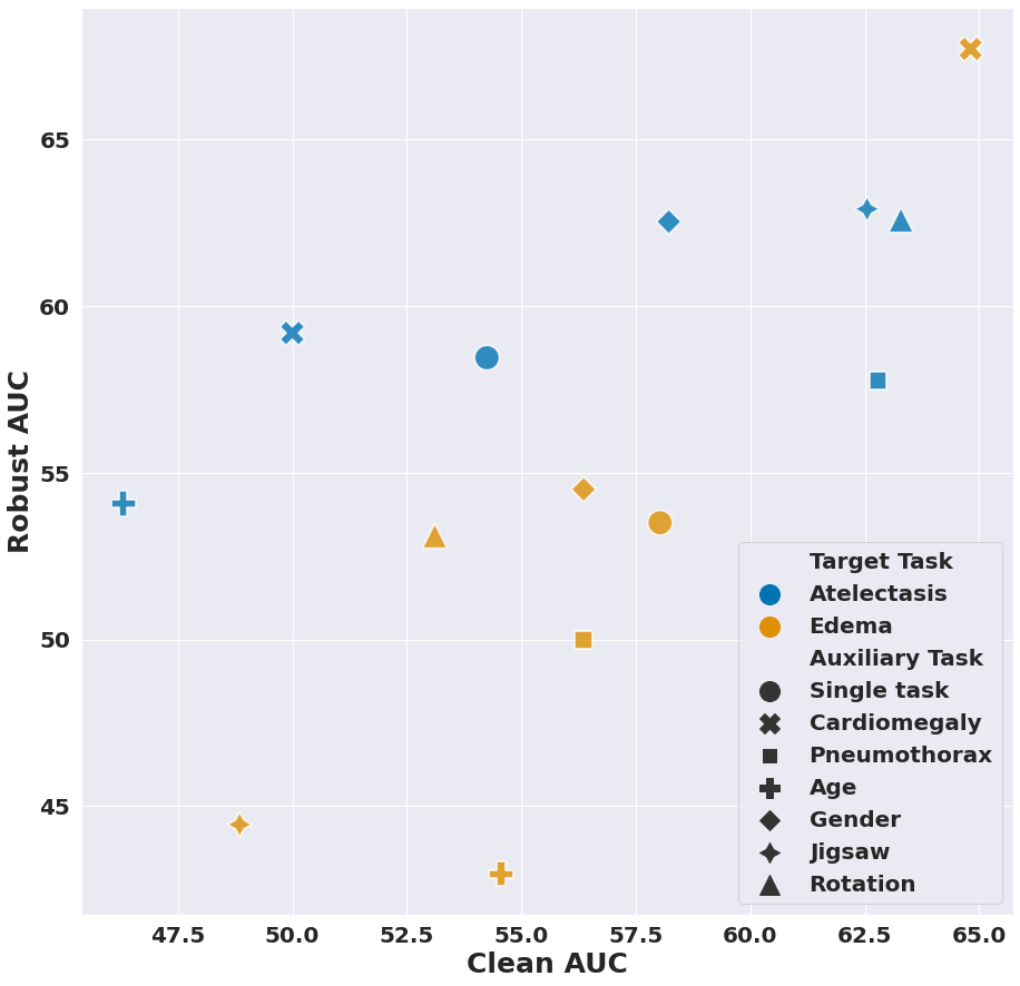
Figure 6: Comparison of different Task Augmentation strategies with single-task models using Adversarial Training; Clean and robust AUC of GAT vs Single task adversarial training to diagnose Atelectasis and Edema pathologies for the NIH dataset

Table 12: Four Different $\mathcal{T}_{i}$ Scenarios: $\mathcal{T}_{1}$ ; standard training, $\mathcal{T}_{2}$ : adversarial training @ Goodfellow, $\mathcal{T}_{3}$ : adversarial training @ Madry, $\mathcal{T}_{4}$ : adversarial training @ Trades (Zhang et al., 2019), and $\mathcal{T}_{5}$ : adversarial training @ Fast(Wong et al., 2020), with 3 different task augmentations and equal weighting strategies.

Scenario	Clean accuracy (%)			Robust accuracy (%)
	Jigsaw	Macro	Rotation	Jigsaw	Macro	Rotation
$\mathcal{T}_{1}$ : Standard training	88.78	93.04	69.67	0.59	0.06	3.18
$\mathcal{T}_{3}$ : Madry AT	64.9	83.00	68.23	20.25	32.16	25.43
$\mathcal{T}_{2}$ : Goodfellow AT	55.01	77.49	42.29	40.5	38.24	34.43
$\mathcal{T}_{4}$ : Trades AT	46.4	60.73	50.24	33.61	42.76	42.05
$\mathcal{T}_{5}$ : Fast AT	52.35	78.18	56.36	19.06	26.56	19.84

C.3 GAT combined with other weighting strategies

We evaluate 5 weighting strategies on Resnet-50 architectures:

1. Equal weights (Equal),

2. Impartial Multi-task Learning (IMTL) (Liu et al., 2021),

3. Multiple Gradient Descent Algorithm (MGDA) (Sener & Koltun, 2018),

4. Gradient Vaccine (GradVac) (Wang et al., 2020),

5. Project Conflicting Gradients (PCGrad) (Yu et al., 2020)

The results in Table 13 uncover that adversarial training using the Macro task yields the best performance in 4 over 5 weighting strategies, and that MGDA weighting strategies yields the best clean and robust accuracy among the weighting strategies (with the MACRO task). MGDA uses multi-objective optimization to converge to the pareto-stationnary for both the tasks we train over. This search algorithm shows that we can attain loss landscapes with high clean and robust performances that greedy gradient algorithms (equal weights, GradVac, PCGrad) fail to uncover.

We used the default hyper-parameters for the weighting strategies. One possible work would be to fine-tune the weighting strategies to the adversarial training setting.

Table 13: Evaluation results of Two Different $\mathcal{T}_{i}$ Scenarios: $\mathcal{T}_{1}$ (standard training), $\mathcal{T}_{2}$ (adversarial training), with 3 different task augmentations and 5 weighting strategies. In bold, the best values for each scenario

Scenario	Weight	Clean accuracy (%)			Robust accuracy (%)
		Jigsaw	Macro	Rotation	Jigsaw	Macro	Rotation
$\mathcal{T}_{1}$	Equal	88.78	93.04	69.67	0.59	0.06	3.18
	GradVac	89.08	93.01	68.42	0.26	0.09	3.81
	IMTL	61.46	93.75	71.24	0.98	0.09	3.81
	GAT [Ours]	41.65	93.89	70.26	0.00	0.24	4.33
	PCGrad	88.85	92.99	69.11	0.69	0.11	3.13
$\mathcal{T}_{2}$	Equal	55.01	77.49	42.29	40.5	38.24	34.43
	GradVac	44.67	64.11	57.71	36.24	35.56	40.17
	IMTL	42.05	69.63	59.61	33.84	48.21	39.93
	MGDA [Ours]	43.99	73.7	56.51	32.95	48.38	36.13
	PCGrad	41.6	63.76	56.38	33.8	44.74	41.59

Hyper-volume.

Hyper-volume is a popular metric to compare different pareto fronts. It only needs a reference point as showed in Fi.7. It calculates the area/volume, which is dominated by the provided set of solutions with respect to a reference point. We use the implementation from the Pymoo library.

We provide in Table LABEL:table:hypervolume the hyper-volume metric of the fronts obtained using each of the weighting strategies (MGDA, IMTL, GV, PCG) we compare. Lower values indicate better solutions. The results confirm that using MGDA for GAT leads to better pareto-fronts.

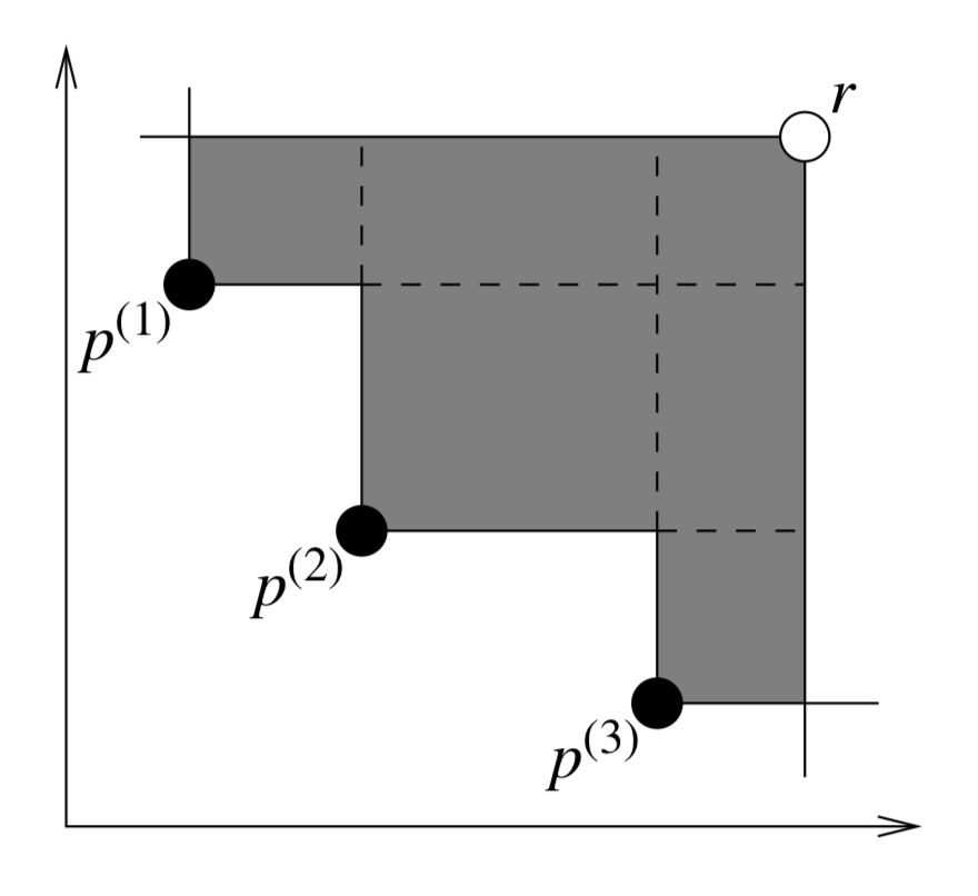
Figure 7: Hypervolume (Fonseca et al., 2006)

Table 14: Hyper-volume of different fronts. Lower values mean better pareto-fronts.

Weight	Hyper-volume
MGDA (OURS)	0.4442
IMTL	0.4534
PCG	0.4679
GV	0.4497

C.4 Impact of number of tasks

We show in Table 15 how robust accuracy of models fluctuate depending on the choice and number of auxiliary tasks. It seems that the Jigsaw task is the most vulnerable and causes significant degradation of the robustness of the model.

Table 15: Impact of the number of tasks on the robust accuracy of models.

Added tasks	Robust accuracy (%)	Number of tasks
Target (No auxiliary task)	39.09	1
Target + Jigsaw	32.95	2
Target + Rotation	36.13	2
Target + Macro	48.38	2
Target + Jigsaw + Rotation	35.45	3
Target + Jigsaw + Macro	16.13	3
Target + Rotation + Macro	56.21	3
Target + Macro + Rotation + Jigsaw	28.24	4

C.5 Adaptive attacks: AutoAttack

We evaluate for all the models of the study the adversarial robustness against AutoAttack. For 3/4 scenarios, adversarial training with task augmentation using Macro tasks outperforms single-task adversarial training.

Table 16: Robust accuracy (%) against AutoAttack of different models adversarially trained with GAT, with 3 different task augmentations, compared to their counterpart single task adversarially trained models. In bold the cases where GAT outperforms single-task AT.

Dataset	Scenario	Auxiliary task
		None	Jigsaw	Macro	Rotation
CIFAR-10	100% Dataset	27.01	29.63	32.54	13.82
	10% Dataset	14.27	11.63	15.00	11.56
	WideResnet28-10	36.29	15.99	34.44	25.72
	WideResNet-70-16	36.29	15.99	34.44	25.72
STL-10	100% Dataset	19.40	12.78	20.02	17.64

C.6 Surrogate attacks

We evaluate in Table 17 the transferability of attacks from a surrogate model to a target model. Both models are trained on the same training dataset.

(1) When the target model has an auxiliary task, the success rate of the attack crafted from a single-task surrogate model drops by 14%. (2) When the surrogate model has an auxiliary task, the success rate against a single task target model drops by 60%.

(1) indicates that the adversarial examples generated to fool a multi-task model actually lie in a loss landscape that is not adversarial for the single task model: The PGD optimization is misguided when multiple tasks are present.

(2) The adversarial examples generated against one single task are actual relevant to models with multiple tasks. It means that multitask learning by itself has the same vulnerable area as the single task-learning, it is just that gradient-based attacks have more difficulty to find them.

Table 17: Evaluation results of Three Different combinations of surrogate models and target models. For each combination, we craft the adversarial examples on the surrogate and evaluate the success rate of the examples on the target models. Both surrogate and target models are trained with standard training.

Target $\rightarrow$	Single Task	Auxiliary Rotation	Auxiliary Jigsaw
Surrogate $\downarrow$	Success rate %
Single Task	98.47	84.55	86.56
Auxiliary Rotation	37.95	98.05	79.86
Auxiliary Jigsaw	37.48	79.35	98.59

References

- Andriushchenko et al. (2020) Andriushchenko, M., Croce, F., Flammarion, N., and Hein, M. Square attack: a query-efficient black-box adversarial attack via random search. In Computer Vision–ECCV 2020: 16th European Conference, Glasgow, UK, August 23–28, 2020, Proceedings, Part XXIII, pp. 484–501. Springer, 2020.
- Cao et al. (2019) Cao, Y., Xiao, C., Cyr, B., Zhou, Y., Park, W., Rampazzi, S., Chen, Q. A., Fu, K., and Mao, Z. M. Adversarial sensor attack on lidar-based perception in autonomous driving. In Proceedings of the 2019 ACM SIGSAC conference on computer and communications security, pp. 2267–2281, 2019.
- Carmon et al. (2019) Carmon, Y., Raghunathan, A., Schmidt, L., Duchi, J. C., and Liang, P. S. Unlabeled data improves adversarial robustness. Advances in Neural Information Processing Systems, 32, 2019.
- Caruana (1997) Caruana, R. Multitask learning. Machine learning, 28(1):41–75, 1997.
- Chen et al. (2020) Chen, T., Liu, S., Chang, S., Cheng, Y., Amini, L., and Wang, Z. Adversarial robustness: From self-supervised pre-training to fine-tuning. In Proceedings of the IEEE/CVF Conference on Computer Vision and Pattern Recognition, pp. 699–708, 2020.
- Cohen et al. (2020) Cohen, J. P., Hashir, M., Brooks, R., and Bertrand, H. On the limits of cross-domain generalization in automated x-ray prediction, 2020.
- Croce & Hein (2020a) Croce, F. and Hein, M. Reliable evaluation of adversarial robustness with an ensemble of diverse parameter-free attacks. In International conference on machine learning, pp. 2206–2216. PMLR, 2020a.
- Croce & Hein (2020b) Croce, F. and Hein, M. Minimally distorted adversarial examples with a fast adaptive boundary attack. In International Conference on Machine Learning, pp. 2196–2205. PMLR, 2020b.
- Croce & Hein (2020c) Croce, F. and Hein, M. Reliable evaluation of adversarial robustness with an ensemble of diverse parameter-free attacks. In International conference on machine learning, pp. 2206–2216. PMLR, 2020c.
- Croce et al. (2020) Croce, F., Andriushchenko, M., Sehwag, V., Debenedetti, E., Flammarion, N., Chiang, M., Mittal, P., and Hein, M. Robustbench: a standardized adversarial robustness benchmark. arXiv preprint arXiv:2010.09670, 2020.
- Desideri (2012) Desideri, J.-A. Multiple-gradient descent algorithm (mgda) for multiobjective optimization. Comptes Rendus Mathematique, 350(5):313–318, 2012. ISSN 1631-073X. doi: https://doi.org/10.1016/j.crma.2012.03.014. URL https://www.sciencedirect.com/science/article/pii/S1631073X12000738.
- Dietterich (1998) Dietterich, T. G. Approximate Statistical Tests for Comparing Supervised Classification Learning Algorithms. Neural Computation, 10(7):1895–1923, 10 1998. ISSN 0899-7667. doi: 10.1162/089976698300017197. URL https://doi.org/10.1162/089976698300017197.
- Dong & Yang (2019) Dong, X. and Yang, Y. Searching for a robust neural architecture in four gpu hours, 2019. URL https://arxiv.org/abs/1910.04465.
- Dong et al. (2018) Dong, Y., Liao, F., Pang, T., Su, H., Zhu, J., Hu, X., and Li, J. Boosting adversarial attacks with momentum. In Proceedings of the IEEE conference on computer vision and pattern recognition, pp. 9185–9193, 2018.
- Engstrom et al. (2017) Engstrom, L., Tran, B., Tsipras, D., Schmidt, L., and Madry, A. Exploring the landscape of spatial robustness, 2017. URL https://arxiv.org/abs/1712.02779.
- Fonseca et al. (2006) Fonseca, C. M., Paquete, L., and López-Ibáñez, M. An improved dimension-sweep algorithm for the hypervolume indicator. 2006 IEEE International Conference on Evolutionary Computation, pp. 1157–1163, 2006.
- Ganesan et al. (2019) Ganesan, P., Rajaraman, S., Long, R., Ghoraani, B., and Antani, S. Assessment of data augmentation strategies toward performance improvement of abnormality classification in chest radiographs. In 2019 41st Annual International Conference of the IEEE Engineering in Medicine and Biology Society (EMBC), pp. 841–844. IEEE, 2019.
- Ghamizi et al. (2019) Ghamizi, S., Cordy, M., Papadakis, M., and Traon, Y. L. Automated search for configurations of convolutional neural network architectures. In Proceedings of the 23rd International Systems and Software Product Line Conference - Volume A, SPLC ’19, pp. 119–130, New York, NY, USA, 2019. Association for Computing Machinery. ISBN 9781450371384. doi: 10.1145/3336294.3336306. URL https://doi.org/10.1145/3336294.3336306.
- Ghamizi et al. (2020) Ghamizi, S., Cordy, M., Gubri, M., Papadakis, M., Boystov, A., Le Traon, Y., and Goujon, A. Search-based adversarial testing and improvement of constrained credit scoring systems. In Proceedings of the 28th ACM Joint Meeting on European Software Engineering Conference and Symposium on the Foundations of Software Engineering, ESEC/FSE 2020, pp. 1089–1100, New York, NY, USA, 2020. Association for Computing Machinery. ISBN 9781450370431. doi: 10.1145/3368089.3409739. URL https://doi.org/10.1145/3368089.3409739.
- Ghamizi et al. (2021) Ghamizi, S., Cordy, M., Papadakis, M., and Traon, Y. L. Adversarial robustness in multi-task learning: Promises and illusions, 2021. URL https://arxiv.org/abs/2110.15053.
- Ghamizi et al. (2022) Ghamizi, S., Cordy, M., Papadakis, M., and Traon, Y. L. Adversarial robustness in multi-task learning: Promises and illusions. Proceedings of the AAAI Conference on Artificial Intelligence, 36(1):697–705, Jun. 2022. doi: 10.1609/aaai.v36i1.19950. URL https://ojs.aaai.org/index.php/AAAI/article/view/19950.
- Gidaris et al. (2018) Gidaris, S., Singh, P., and Komodakis, N. Unsupervised representation learning by predicting image rotations. arXiv preprint arXiv:1803.07728, 2018.
- Gong et al. (2020) Gong, C., Ren, T., Ye, M., and Liu, Q. Maxup: A simple way to improve generalization of neural network training, 2020. URL https://arxiv.org/abs/2002.09024.
- Goodfellow et al. (2014a) Goodfellow, I. J., Shlens, J., and Szegedy, C. Explaining and harnessing adversarial examples. arXiv preprint arXiv:1412.6572, 2014a.
- Goodfellow et al. (2014b) Goodfellow, I. J., Shlens, J., and Szegedy, C. Explaining and harnessing adversarial examples. arXiv preprint arXiv:1412.6572, 2014b.
- Gowal et al. (2021) Gowal, S., Rebuffi, S.-A., Wiles, O., Stimberg, F., Calian, D. A., and Mann, T. A. Improving robustness using generated data. Advances in Neural Information Processing Systems, 34, 2021.
- He et al. (2016) He, K., Zhang, X., Ren, S., and Sun, J. Identity mappings in deep residual networks. In European conference on computer vision, pp. 630–645. Springer, 2016.
- Hendrycks et al. (2019) Hendrycks, D., Mazeika, M., Kadavath, S., and Song, D. Using self-supervised learning can improve model robustness and uncertainty. Advances in neural information processing systems, 32, 2019.
- Ho et al. (2020) Ho, J., Jain, A., and Abbeel, P. Denoising diffusion probabilistic models, 2020. URL https://arxiv.org/abs/2006.11239.
- Irvin et al. (2019) Irvin, J., Rajpurkar, P., and al. Chexpert: A large chest radiograph dataset with uncertainty labels and expert comparison, 2019.
- Jaggi (2013) Jaggi, M. Revisiting Frank-Wolfe: Projection-free sparse convex optimization. In Dasgupta, S. and McAllester, D. (eds.), Proceedings of the 30th International Conference on Machine Learning, volume 28 of Proceedings of Machine Learning Research, pp. 427–435, Atlanta, Georgia, USA, 17–19 Jun 2013. PMLR. URL https://proceedings.mlr.press/v28/jaggi13.html.
- Kaisa (1999) Kaisa, M. Nonlinear Multiobjective Optimization, volume 12 of International Series in Operations Research & Management Science. Kluwer Academic Publishers, Boston, USA, 1999.
- Kim (2020) Kim, H. Torchattacks: A pytorch repository for adversarial attacks. arXiv preprint arXiv:2010.01950, 2020.
- Klingner et al. (2020) Klingner, M., Bar, A., and Fingscheidt, T. Improved noise and attack robustness for semantic segmentation by using multi-task training with self-supervised depth estimation. In Proceedings of the IEEE/CVF Conference on Computer Vision and Pattern Recognition Workshops, pp. 320–321, 2020.
- Krizhevsky et al. (2009) Krizhevsky, A., Hinton, G., et al. Learning multiple layers of features from tiny images. 2009.
- Kurakin et al. (2016) Kurakin, A., Goodfellow, I., and Bengio, S. Adversarial machine learning at scale. arXiv preprint arXiv:1611.01236, 2016.
- Liu et al. (2021) Liu, L., Li, Y., Kuang, Z., Xue, J., Chen, Y., Yang, W., Liao, Q., and Zhang, W. Towards impartial multi-task learning. ICLR, 2021.
- Ma et al. (2021) Ma, X., Niu, Y., Gu, L., Wang, Y., Zhao, Y., Bailey, J., and Lu, F. Understanding adversarial attacks on deep learning based medical image analysis systems. Pattern Recognition, 110:107332, 2021. ISSN 0031-3203. doi: https://doi.org/10.1016/j.patcog.2020.107332. URL https://www.sciencedirect.com/science/article/pii/S0031320320301357.
- Madry et al. (2017a) Madry, A., Makelov, A., Schmidt, L., Tsipras, D., and Vladu, A. Towards deep learning models resistant to adversarial attacks. arXiv preprint arXiv:1706.06083, 2017a.
- Madry et al. (2017b) Madry, A., Makelov, A., Schmidt, L., Tsipras, D., and Vladu, A. Towards deep learning models resistant to adversarial attacks. arXiv preprint arXiv:1706.06083, 2017b.
- Mao et al. (2020) Mao, C., Gupta, A., Nitin, V., Ray, B., Song, S., Yang, J., and Vondrick, C. Multitask learning strengthens adversarial robustness. In Computer Vision - ECCV 2020 - 16th European Conference, Glasgow, UK, August 23-28, 2020, Proceedings, Part II, volume 12347 of Lecture Notes in Computer Science, pp. 158–174. Springer, 2020. doi: 10.1007/978-3-030-58536-5“˙10. URL https://doi.org/10.1007/978-3-030-58536-5_10.
- Moosavi-Dezfooli et al. (2018) Moosavi-Dezfooli, S.-M., Fawzi, A., Uesato, J., and Frossard, P. Robustness via curvature regularization, and vice versa, 2018. URL https://arxiv.org/abs/1811.09716.
- Noroozi & Favaro (2016) Noroozi, M. and Favaro, P. Unsupervised learning of visual representations by solving jigsaw puzzles. In European conference on computer vision, pp. 69–84. Springer, 2016.
- Rebuffi et al. (2021) Rebuffi, S.-A., Gowal, S., Calian, D. A., Stimberg, F., Wiles, O., and Mann, T. A. Data augmentation can improve robustness. Advances in Neural Information Processing Systems, 34, 2021.
- Ronneberger et al. (2015) Ronneberger, O., Fischer, P., and Brox, T. U-net: Convolutional networks for biomedical image segmentation. In International Conference on Medical image computing and computer-assisted intervention, pp. 234–241. Springer, 2015.
- Ruder (2017) Ruder, S. An overview of multi-task learning in deep neural networks. arXiv preprint arXiv:1706.05098, 2017.
- Schmidt et al. (2018) Schmidt, L., Santurkar, S., Tsipras, D., Talwar, K., and Madry, A. Adversarially robust generalization requires more data. Advances in neural information processing systems, 31, 2018.
- Sener & Koltun (2018) Sener, O. and Koltun, V. Multi-task learning as multi-objective optimization. In Bengio, S., Wallach, H., Larochelle, H., Grauman, K., Cesa-Bianchi, N., and Garnett, R. (eds.), Advances in Neural Information Processing Systems, volume 31. Curran Associates, Inc., 2018. URL https://proceedings.neurips.cc/paper/2018/file/432aca3a1e345e339f35a30c8f65edce-Paper.pdf.
- Shafahi et al. (2019) Shafahi, A., Najibi, M., Ghiasi, M. A., Xu, Z., Dickerson, J., Studer, C., Davis, L. S., Taylor, G., and Goldstein, T. Adversarial training for free! Advances in Neural Information Processing Systems, 32, 2019.