Renormalized density matrix downfolding: a rigorous framework in learning emergent models from ab initio many-body calculations

Abstract

We present a generalized framework, renormalized density matrix downfolding (R-DMD), to derive systematically improvable effective models from ab initio calculations. This framework moves beyond the common role of ab initio calculations as calculating the parameters of a proposed Hamiltonian. Instead, R-DMD provides the capability to decide whether a given effective Hilbert space can be identified from the ab initio data and assess the relative quality of ansatz Hamiltonians. Any method of ab initio solution can be used as a data source, and as the ab initio solutions improve, the resultant model also improves. We demonstrate the framework in an application to the downfolding of a hydrogen chain to a spin model, in which we find the interatomic separations for which a nonperturbative mapping can be made, and compute a renormalized spin model Hamiltonian that quantitatively reproduces the ab initio dynamics.

A fundamental objective of condensed matter physics is to classify states of matter that emerge from the common makeup of electrons and nuclei. The program for doing this was laid out in the renormalization group approach [1, 2, 3]. A crucial tool in serving this objective is the use of effective Hamiltonians/Lagrangians, which are often written in terms of effective degrees of freedom, such as quasiparticles. However, applications where renormalization group can be applied non-perturbatively are few and far between, and represent a major challenge in the study of materials such as the cuprates [4, 5, 6, 7, 8, 9, 10, 11, 12, 13, 14], pyrochlore iridates [15, 16], spin liquid candidates [17, 18, 19], and twisted bilayer graphene [20, 21], and these materials appear to be too complex for the effective Hamiltonian to be fully determined by experiment.

Over the past few years, it has been shown that many-body approaches to the ab initio problem can often obtain reasonably high accuracy solutions even for strongly correlated systems. Approaches such as multi-reference quantum chemistry methods [22, 23, 24, 25], various flavors of quantum Monte Carlo [26, 27, 28, 29], and density matrix renormalization group [4, 30, 31] use heuristics to achieve systematically improvable approximations of the ground states. Recently, it has been shown that converged results can be obtained using these techniques [32, 33, 34, 35]; however, these studies are limited to small system sizes of 30 or fewer electrons. However, up to now, there is no method to systematically connect these high-accuracy many-body methods to lower energy effective theories, which is necessary to study longer length scales and larger systems.

The state of the art in downfolding from ab initio calculations is to construct an effective Hamiltonian from density functional theory, with interactions added either through a constrained random phase approximation (cRPA) [36, 37] or $GW$ [38, 39, 11]. However, these downfolding methods based on DFT are limited by their ingredients, and for strongly correlated systems, their accuracy is often poor [40, 33].

We present a rigorous, non-perturbative, method to compute downfolded models using accurate many-body ab initio solutions, which we term renormalized density matrix downfolding (R-DMD). The quality of the model is based upon reproducing the ab initio data, so all choices in constructing the model can be systematically improved based on obtaining the best fit to the data. In this sense of reproducing ab initio data, the method is amenable to machine learning methods, especially feature selection techniques. Renormalization of physical quantities, such as effective spin, is obtained as a result of the downfolding and can be dynamical, in contrast to standard techniques [41]. We demonstrate the method using the strongly correlated hydrogen chain, in which we map the regions of phase space in which the ab initio system can be mapped onto a spin model, and construct a complete nonperturbative renormalization to a spin model where possible.

I The landscape of downfolding techniques

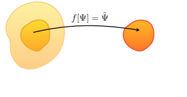
Figure 1: A 1-1 mapping between the ab initio emergent low-energy Hilbert space and the model Hilbert space enables ab initio dynamics to be reproduced by an effective model.

Table 1: A unified comparison of common approaches to downfolding to reduced Hamiltonians.

Method	$\mathcal{LE}$ choice	$f$	$H_{\text{eff}}$
DFT+cRPA	active orbitals	bare	$H_{\text{KS}}+H_{\text{DC}}+H_{\text{cRPA}}$
Shrieffer-Wolff transformation	Eigenstates of $H_{0}$		Perturbatively renormalized
Canonical transformation	rotation	bare	In principle exact, but usually truncated
Spectral fitting	eigenstates of $H_{ab}$	closest energy	Best fit to ab initio data
DMD	eigenstates of $H_{ab}$	bare	Best fit to ab initio data
R-DMD	eigenstates of $H_{ab}$	closest match	Best fit to ab initio data

To help understand the choices in downfolding, in Fig 1, we outline the general procedure. A subspace of the ab initio Hilbert space $\mathcal{H}_{ab}$, called $\mathcal{LE}$ is chosen to represent the low-energy space. A 1-1 mapping $f$ is constructed between $\mathcal{LE}$ and some model Hilbert space $\mathcal{H}_{\text{model}}$. We start with the following general considerations, which are easy to show:

1. If $\mathcal{LE}$ is spanned by a set of energy eigenstates, then dynamics within that space are closed (i.e., an effective Hamiltonian is sufficient). If it is not, then the resulting dynamics on the model space must have frequency dependence.

2. For any choice of the 1-1 mapping $f$, if (1) is satisfied and $\langle\Psi_{i}|H_{ab}|\Psi_{j}\rangle=\langle f[\Psi_{i}]|H_{\mathrm{model}}|f[\Psi_{j}]\rangle$ $\forall\,\Psi_{i},\Psi_{j}\in\mathcal{LE}$, the dynamics in the model system exactly match the dynamics of the ab initio system.

3. $f$ can be constructed in any way, as long as it is 1-1 and (2) is true. However, some constructions of $f$ result in more complex effective Hamiltonians than others.

4. Note also that $\mathcal{LE}$ must be the same dimension as $\mathcal{H}_{\text{model}}$; otherwise, a 1-1 mapping does not exist.

Note that this paradigm can be adjusted and modified; if $\mathcal{LE}$ is smaller than $\mathcal{H}_{\text{model}}$, then a mapping can be made, and as long as the effective Hamiltonian satisfies (2), the dynamics are preserved. To prevent extraneous low-energy states in the model space, additional terms might be necessary in the model Hamiltonian $H_{\text{model}}$. Also, depending on the choice of $\mathcal{LE}$, it may or may not map onto a simple model Hilbert space $\mathcal{H}_{\text{model}}$. The downfolding process is actually one of design; there are many correct ways to do it but only some of them will result in simple and interpretable models.

DFT+cRPA: In this technique [36], a set of correlated one-particle orbitals (“active orbitals”) is chosen, and the screened Coulomb interaction between them is evaluated. Because $\mathcal{LE}$ is chosen based on active orbitals, it is not closed under the operation of the Hamiltonian, and a frequency-dependent interaction emerges. For the problem considered here (downfolding onto a spin model), a straightforward application of DFT+cRPA is elusive.

Schrieffer-Wolff transformation [42, 43] is a venerable perturbative method that requires that the projected subspace be energetically separated from the rest of the Hilbert space. For this reason, for the case of the hydrogen chain to spin model mapping, this method is expected to work well for large interatomic separations. As we shall show, it is possible to map the low energy spectrum of the hydrogen chain onto a spin model well outside the perturbative regime.

Spectral fitting is a technique that is similar to the current method, in that it uses reference ab initio calculations. In this method, a model is assumed and the parameters are varied to best represent the eigenenergies of the model. A common application of this method is the derivation of the hopping parameters in tight-binding models without wannierization of the Kohn-Sham orbitals, but simply through fitting to either experiment [44] or Kohn-Sham spectra [45]. In contrast to cRPA and Schrieffer-Wolff, such a method is nonperturbative; however, it requires eigenenergies to be matched to one another. As we shall show, it is not necessarily the case that states with the same energy actually correspond to states with similar properties, so a criterion based solely on energy may scramble the physics.

Density matrix downfolding (DMD) [46, 47, 48] is a method that attempts to overcome some of the issues with spectral fitting regarding the properties of the wave function, and also does not require one to obtain exact eigenstates. In this method, one matches the expectation value of the Hamiltonian between the model and ab initio states. However, it does not ensure a 1-1 mapping between the two spaces.

II Renormalized density matrix downfolding

In the new method, we aim to use high-accuracy ab initio data to choose the low-energy space, construct the 1-1 mapping, and to fit the effective Hamiltonian. This technique is non-perturbative and based on high quality ab initio solutions, and overcomes the issues of spectral fitting and density matrix downfolding. Because the 1-1 map is constructed explicitly, R-DMD can also detect when a mapping is possible or not, thus allowing us to evaluate the appropriateness of a model, a capability that most downfolding methods lack. A summary of the strategy is as follows.

1. In this work, $\mathcal{LE}$ is selected based on clustering in a wave function descriptor space. This is done for the hydrogen chain case to correctly identify spin excitations versus charge excitations. A simple energy cutoff would not work. We believe this to be a powerful strategy that encompasses many options; for example, in graphene, one might wish to separate the $p_{z}$ bands from the others, which would be achieved by evaluating the occupation number on the $p_{z}$ states.

2. The key innovation of R-DMD is to construct the 1-1 mapping $f$ not based on exact similarity between model and ab initio states, but approximate similarity. This is intermediate between a method like spectral fitting, which makes no guarantees that the physics of the model resembles the ab initio, and methods such as DMD or DFT+cRPA, which require the model to be written in terms of the bare electrons, resulting in complex Hamiltonians. This choice also improves the fitting process significantly versus spectral fitting. The effective model need not be solved, unlike spectral fitting.

3. With $\mathcal{LE}$ chosen and $f$ constructed, the Hamiltonian parameters are simply fit to minimize the deviation between the model eigenenergies and the ab initio eigenenergies.

III Constructing the ab initio data set

We use real-space variational Monte Carlo (VMC) to obtain approximate many-body wave functions for the eigenstates of the ab initio Hamiltonian,

$$H_{ab}=\sum_{iI}\left(-\frac{1}{2}\nabla_{i}^{2}-\frac{Z_{I}}{\left|\mathbf{r}_{i}-\mathbf{x}_{I}\right|}\right)+\sum_{i\neq j}\frac{1}{\left|\mathbf{r}_{i}-\mathbf{r}_{j}\right|}.$$ (1)

The trial wave functions take a multi-Slater-Jastrow form,

$$\Psi_{T}(\mathbf{r}_{1},\mathbf{r}_{2},\cdots,\mathbf{r}_{N}) =e^{J(\mathbf{r}_{1},\mathbf{r}_{2},\cdots,\mathbf{r}_{N})}$$

$$\times\sum_{k}c_{k}D^{\uparrow}_{k}(\chi_{i\uparrow}(\mathbf{r}_{j}))D^{\downarrow}_{k}(\chi_{i\downarrow}(\mathbf{r}_{j})),$$ (2)

where $\mathbf{r}_{i}$ and $\mathbf{x}_{I}$ represent the real-space coordinates of the $i$th electron and $I$th ion. The multi-Slater expansion $\sum_{k}c_{k}D^{\uparrow}_{k}(\chi_{i\uparrow}(\mathbf{r}_{j}))D^{\downarrow}_{k}(\chi_{i\downarrow}(\mathbf{r}_{j}))$, was generated using a multi-reference quantum chemistry method, restricted Hartree-Fock (RHF) + complete active space self-consistent field (CASSCF) [23]. We started with RHF and optimized molecular orbitals variationally with a single Slater determinant as the ground state ansatz. Then, in state-averaged CASSCF(8, (4, 4)), we chose an active space that includes the first eight molecular orbitals and all the electrons, constrained in the $S_{z}=0$ sector. The CASSCF ansatzes for the eigenstates are expansions of determinants given by all the possible excitations within the active space. The molecular orbitals $\chi_{i\sigma}({\mathbf{r}})$ were parameterized using correlation consistent triple-zeta basis set [49], which includes up to the $3d$ orbitals of hydrogen atoms. In the state-averaged CASSCF calculation, the coefficients $c_{k}$ and $\chi_{i\sigma}(\mathbf{r})$ are optimized to minimize the cost function, which is chosen as the energy averaged over the first $m$ eigenstates. Here, we chose $m=400$ based on the allowed computational resources. The trial wave functions for all the excited states contain the same fixed Jastrow function $e^{J}$ that includes electron-ion and electron-electron correlations, defined in Ref. [50]. The Jastrow function $J(\mathbf{r}_{1},\cdots,\mathbf{r}_{N})$ was optimized for the ground state wave function. We checked that this approximation does not change the derived model, but the model parameters can be improved with more accurate ab initio wave functions.

The training data set for detecting the emergent low-energy Hilbert space $\mathcal{LE}$ is built with the following descriptors of the ab initio eigenstates:

• the energy expectation value:

  $E[\Psi_{a}]=\bra{\Psi_{a}}H_{\text{{ab}}}\ket{\Psi_{a}}$,

• the $l$th-nearest-neighbor hopping, $l=1,\,2,\,3$:

  $d_{t_{l}}[\Psi_{a}]=\sum_{i,\sigma}\bra{\Psi_{a}}c_{i\sigma}^{\dagger}c_{i+l\sigma}+c_{i+l\sigma}^{\dagger}c_{i\sigma}\ket{\Psi_{a}}$,

• the total double occupancy:

  $d_{U}[\Psi_{a}]=\sum_{i}\bra{\Psi_{a}}n_{i\uparrow}n_{i\downarrow}\ket{\Psi_{a}},~{}n_{i\sigma}=c^{\dagger}_{i\sigma}c_{i\sigma}$,

• the spin-spin correlation:

  $d_{J}[\Psi_{a}]=\sum_{\langle i,j\rangle}\bra{\Psi_{a}}\mathbf{S}_{i}\cdot\mathbf{S}_{j}\ket{\Psi_{a}}$,

where $c^{\dagger}_{i\sigma}$($c_{i\sigma}$) creates(annihilates) an electron in orbital $\phi_{i\sigma}$ of the minimal basis set (see appendix A for details in constructing the minimal basis set). $\mathbf{S}_{i}=\sum_{i,\alpha\alpha^{\prime}}c^{\dagger}_{i\alpha}\boldsymbol{\sigma}_{\alpha\alpha^{\prime}}c_{i\alpha^{\prime}}$, where $\boldsymbol{\sigma}=(\sigma_{x},\sigma_{y},\sigma_{z})$ are the spin $1/2$ Pauli matrices.

IV Selection of $\mathcal{LE}$ via clustering

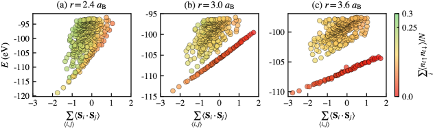
Figure 2: A low-energy space is assignable when there are distinguishable clusters of energy eigenstates in an extended descriptor space. Each point is an energy eigenstate of an 8-atom hydrogen chain. The lines of states in which energy increases roughly linearly with $\sum_{\langle i,j\rangle}\langle\mathbf{S}_{i}\cdot\mathbf{S}_{j}\rangle$ can be mapped 1-1 to a spin Hilbert space. The statistical uncertainties are of order .01 for both quantities, and much smaller than the symbols.

In Fig 2, we show the results of the ab initio solutions of the 8-atom hydrogen chain. Starting from the large separation distance of $r=3.6\,a_{\mathrm{B}}$ (panel (c)), one can easily identify spin-like excitations, in which the double occupancy is low, and the energy varies approximately linearly with the spin correlation $d_{J}$, as one would expect for a Heisenberg-like model. At higher energies, one can see the charge excitations, which have significant double occupancy. As the separation is decreased, the double occupancy in the spin excitations increases, and the charge excitations are closer to energy; however, at $r=3.0\,a_{\mathrm{B}}$, the two groups are still visible by eye. Finally, by $r=2.4\,a_{\mathrm{B}}$, still before the metal-insulator transition, the charge and spin excitations have merged and are not distinguishable except for a few states at very low energy.

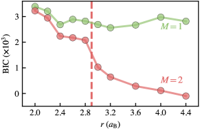
Figure 3: Detection of clusters using a Gaussian mixture model. Above $2.9\,a_{\mathrm{B}}$, there is a significant improvement in the Bayesian information criterion (BIC) for two clusters ($M=2$), indicating the presence of two classes of eigenstate.

An obvious choice for $\mathcal{LE}$ is to use an energy cutoff, as is common in the renormalization group. A problem with this choice is demonstrated in Fig 2(b) and (c), in which there are clear groups of eigenstates when the spin-spin, double occupancy, and energy are considered, but these states overlap in energy. Only when the charge excitations merge with the spin excitations are there not distinguishable spin and charge sectors. While this can be seen by eye for a simple system like this, to systematically classify the eigenstates, we used a Gaussian mixture model (GMM). The GMM is a probabilistic model that assumes a set of descriptors $\mathbf{d}$ of size $n$ is described by a mixture of $M$ Gaussian distributions [51], In particular, it allows for the clusters to be highly anisotropic, as they are in the case here. In this work, we used the machine learning package scikit-learn [52] to determine the distribution with full rank covariance matrices. In the case of the hydrogen chain, $\mathbf{d}$ includes all the descriptors listed in section III. We find that the energy, double occupancy, and spin correlations are the most relevant descriptors; adding more does not change the results of the clustering algorithm.

In order to compute the number of optimal clusters of eigenstates, we chose to use the Bayesian information criterion (BIC) to measure the accuracy of the GMM [53] and apply the heuristic elbow criterion [54] to determine $M$ in the GMM when clustering the eigenstates. The BIC score penalizes the sample size and the total number of parameters to avoid overfitting, so that we are able to detect emergence of disjoint eigenstate clusters that can be assigned to a low-energy space. With this method, $\mathcal{LE}$ is not dictated by an energy cutoff, but instead, an extended descriptor space (energy, spin-spin correlation, and double occupancy) is necessary for it to be detected.

Fig. 3 shows the BIC scores of one- and two-cluster GMMs, for hydrogen chains with interatomic separations $r\geq 2.0\,a_{\mathrm{B}}$, obtained using all the descriptors available. The decrease in BIC for a two-cluster GMM at $3.0\,a_{\mathrm{B}}$ clearly shows that the ab initio eigenstates can be assigned to two groups (the spin- and charge-like excitations). According to this metric, the spin excitations merge into the charge excitations at around $3.0\,a_{\text{B}}$, i.e., an interatomic separation that is unrelated to the ground state metal-insulator transition, indicating the formation of a complex correlated state without a well-separated magnetic spectrum. Note that distinct spin and charge sectors exist even when the double occupancy of the ground state is quite large; at $3.0\,a_{\mathrm{B}}$, it is almost half the noninteracting value of 0.25 in the ground state.

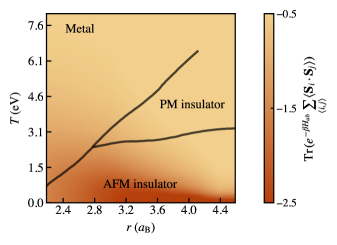
Figure 4: An approximate phase diagram for the hydrogen chain. The colors represent the thermal expectation values of the spin-spin correlations, computed using the ab initio eigenstates of the 8-atom chain. The phase boundaries were sketched based on the values of spin-spin correlations.

We will note here that the selection method is ultimately justified by the quality of $H_{\text{eff}}$. It is an interesting avenue of future research, for more complex systems, whether clusters represent the best partitioning or whether there are more effective methods. The key contribution of this work is that we now have a systematic way of internally assessing one method versus another for any system.

The presence or absence of distinguishable clusters correlates with physics in this system. In Fig 4, an approximate phase diagram is shown. The point at which the clusters become indistinct ($2.8\,a_{\mathrm{B}}$) corresponds to the point at which the paramagnetic insulator phase disappears in the phase diagram, and a metallic antiferromagnet appears.

V Construction of the 1-1 mapping $f$

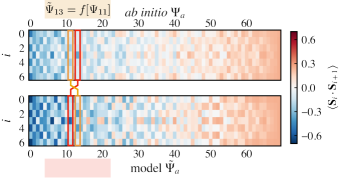
Figure 5: The optimal 1-1 mapping $\tilde{\Psi}=f[\Psi]$ between the ab-initio and model eigenstates: the local spin correlation of the many-body eigenstates at $r=3.0\,a_{\text{B}}$. The model eigenstates are eigenstates of the Heisenberg model. States (columns) are labeled according to their energies and matched according to the similarity of the local descriptors (rows). For example, $\Psi_{11}$ is mapped to model state $\tilde{\Psi}_{13}$ (highlighted in yellow boxes), and $\Psi_{13}$ is mapped to $\tilde{\Psi}_{11}$ (red boxes).

Our ultimate criterion is that the ab initio Hamiltonian operator is reproduced in the model, i.e., $H_{\text{eff}}$ satisfies

$$\langle\Psi_{i}|H_{ab}|\Psi_{j}\rangle=\langle f[\Psi_{i}]|H_{\mathrm{eff}}|f[\Psi_{j}]\rangle,$$ (3)

for all $\Psi_{i},\Psi_{j}\in\mathcal{LE}$, then the dynamics in the model system are the same as the ab initio. This requires a functional mapping $f$ between the indices of the two operators. $f$ can be chosen arbitrarily so long as Eqn 3 is satisfied. Therefore, one can choose any heuristic, so long as Eqn 3 can be matched.

In the case of mapping the hydrogen chain to a spin model, we take advantage of a simplification that occurs since we are interested in finding the best Heisenberg model. The energy eigenstates of the Heisenberg model are identical independent of the value of $J$. We thus associate the ab initio eigenstate $\Psi_{a}$ with the model eigenstate $\tilde{\Psi}_{b}$ based on a similarity of the local spin-spin correlations. An example is shown in Fig 5. We construct a vector of descriptors in first principles $d_{ai}=\langle\Psi_{a}|\mathbf{S}_{i}\cdot\mathbf{S}_{i+1}|\Psi_{a}\rangle$ and the equivalent for the model space. Then we compute the $N\times N$ distance matrix $D_{ab}=\sum_{i}(d_{ai}-\tilde{d}_{bi})^{2}$. The assignment problem is then solved using the linear assignment method [55].

In more complex situations, this method can be extended as follows. Define

$$D_{ij}=\langle\Psi_{i}|\hat{D}|\Psi_{j}\rangle$$ (4)

and

$$\tilde{D}_{ij}=\langle\tilde{\Phi}_{i}|\hat{\tilde{D}}|\tilde{\Phi}_{j}\rangle,$$ (5)

for operators $\hat{D}$ in the ab initio space, corresponding operator $\hat{\tilde{D}}$ in the model space, and $\tilde{\Phi}_{i}$ some orthogonal basis in the model space. Then, the optimal assignment can be given by choosing a rotation matrix $R$ such that the objective function

$$\lVert D-R^{T}\tilde{D}R\rVert^{2}$$ (6)

is minimized. Our simpler strategy above is equivalent to this with the constraint that the rotation matrix can only interchange eigenstates of the Heisenberg model, not create superpositions of them.

We will also note here that $f$ could be assigned in other ways; it is an interesting research avenue to explore what heuristics result in the most accurate and simple $H_{\text{eff}}$ for common systems. One could potentially apply machine learning tools to select the correct assignment of states for a given criterion of simplicity and accuracy of $H_{\text{eff}}$. As we shall show later, the method we use here results in accurate Heisenberg models for the hydrogen chain. We expect, since it is physically motivated, methods such as the one presented here will be useful.

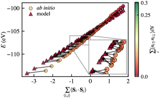
Figure 6: Optimal Heisenberg model with mapping determined from Fig 5 with $r=3.0\,a_{\mathrm{B}}$. The energy of the model states is computed with the optimal Heisenberg model. A perfect mapping would have model and ab initio states with exactly the same energy. The mapping renormalizes the spin operator explicitly for each wave function in $\mathcal{LE}$; the horizontal distance is the renormalization of spin. In the figure, the black arrows indicate this state-wise renormalization of the spin operator.

The result of the assignment is shown in Fig 6. At this interatomic separation, the effective spins in the model are quite different from the ab initio spins. From this assignment, one can see the effects of renormalization on the model description of the antiferromagnetic ground state, and very little in the ferromagnetic highest energy state, since the mapped model spin correlations are very different for the antiferromagnetic state, while very similar for the ferromagnetic state. The mapping is not a constant renormalization of the magnitude of the spin operators; on the contrary, the spin moment measured in the model space is related to the ab initio spin by a state-dependent factor. Without constructing the mapping explicitly, it would be very difficult to guess the spin renormalization even in this simple case.

VI Determination of $H_{\mathrm{eff}}$

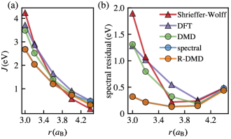
Figure 7: (a) The derived $J$ values and (b) the spectral residual evaluated using Schrieffer-Wolff transformation, DFT, DMD, spectral-fitting DMD (spectral), and R-DMD versus the interatomic separation.

If $H_{\text{eff}}$ satisfies Eqn 3, then the dynamics in the model system are the same as the ab initio. One can see this easily because

$$\exp(-iH_{ab}t)|\Psi\rangle=f^{-1}\left[\exp(-iH_{\mathrm{eff}}t)|f[\Psi]\rangle\right].$$ (7)

Because we are matching energy eigenstates to energy eigenstates, the off-diagonal elements of Eqn 3 are automatically satisfied. We thus fit $J$ and $E_{0}$ to minimize the loss function

$$\sum_{a}\left(J\langle f[\Psi_{a}]|\tilde{\mathbf{S}}_{i}\cdot\tilde{\mathbf{S}}_{j}|f[\Psi_{a}]\rangle+E_{0}-\langle\Psi_{a}|H_{ab}|\Psi_{a}\rangle\right)^{2},$$ (8)

where $\tilde{\mathbf{S}}_{i}$ are spin-1/2 operators in the spin Hilbert space (not the ab initio space).

In Fig 7, we compare the derived $J$ and the error compared to the underlying ab initio data as a function of interatomic spacing. We compare to the DFT-computed $J$ from broken-symmetry magnetic states, the Schreiffer-Wolf perturbative calculation from an effective $t-U$ model (see appendix B), density matrix downfolding (DMD), and matching the spectrum without matching the properties of the states (spectral). Perturbative methods such as Schreiffer-Wolf work well for large interatomic separation $r$, but overestimate $J$ at smaller $r$. Unlike R-DMD, perturbative techniques also give no indication of their accuracy/applicability at lower interatomic separations. Broken symmetry DFT calculations are similar, both in the lack of indication of applicability and in the poor calculation of the $J$ term at lower $r$ due to inaccuracies in the density functional. In this simple case, spectral mapping is very similar to R-DMD, where the matching function is the minimum difference between eigenstate energies. However, in the general case, spectral mapping would require many diagonalizations of the effective Hamiltonian, while R-DMD does not require the effective Hamiltonian to be diagonalized at all.

VII Conclusion

We have presented a new approach to the determination of multiscale models, called renormalized density matrix downfolding (R-DMD), bringing the derivation of electronic models to the same footing as atomic force field models. This approach is systematically improvable in two senses: the underlying data can be improved systematically by considering progressively more accurate solutions of the ab initio problem, and the effective Hilbert space and Hamiltonian can be systematically improved to better represent the underlying ab initio data. Note that this method does not require exact energy eigenstates, so long as the ab initio data is a superposition of the eigenstates that span $\mathcal{LE}$, nor does it require the model Hamiltonian to be diagonalized. Renormalization of quantum operators is determined as a byproduct of the procedure and is explicitly constructed.

R-DMD is a flexible framework, in which the mapping function $f$ and the choice of the low-energy space $\mathcal{LE}$ can be selected at will to produce the most accurate and simple resultant Hilbert space and Hamiltonian. Eqn 3 gives a variational criterion for constructing low-energy models. The selection of $\mathcal{LE}$ and $f$ are arbitrary as long as $\mathcal{LE}$ is spanned by eigenstates and $f$ is 1-1. It is also possible to adapt R-DMD to treat systems in which $\mathcal{LE}$ is not closed under the application of $H_{ab}$. In this case, the energy-conserving Hamiltonian framework used here would need to be extended to a Lagrangian or Linbladian description in the model space.

VIII Acknowledgements

The initial contributions of Y.C. in performing calculations, generating the data, and developing the theory, and the contributions of L.K.W. in supervising, writing, and creating the theory were supported by the U.S. Department of Energy, Office of Science, Office of Basic Energy Sciences, Computational Materials Sciences Program, under Award No. DE-SC0020177. The contribution of Y.C. in writing was funded by the Abrahams Postdoctoral Fellowship from the Center for Materials Theory, Department of Physics & Astronomy at Rutgers University. The contributions of S.J. in developing the method of systematically constructing the 1-1 mapping $f$ and writing were supported by the National Science Foundation under Grant No. DGE-1922758. This work made use of the Illinois Campus Cluster, a computing resource that is operated by the Illinois Campus Cluster Program (ICCP) in conjunction with the National Center for Supercomputing Applications (NCSA) and which is supported by funds from the University of Illinois at Urbana-Champaign. This research used resources of the Oak Ridge Leadership Computing Facility at the Oak Ridge National Laboratory, which is supported by the Office of Science of the U.S. Department of Energy under Contract No. DE-AC05-00OR22725.

Appendix A Finding a minimal basis set of a $\mathcal{LE}$

In general, constructing a localized basis set for a set of ab initio eigenstates is not necessary — one could optimize the basis when determining the $\mathcal{LE}$, enforcing the effective Hamiltonian to be as compact as possible. However, in the case of the 8-atom hydrogen chain, we found using a localized basis set constructed in the following way sufficiently good for obtaining compact models in hydrogen chains. Note that one might need to use generalized principal components of two-body or even higher-order reduced density matrices if one is to describe higher-order interactions. Since the descriptors evaluated on the basis sets are only used for determining the 1-1 mapping $f$, as long as $f$ stays topologically the same, the choice of the basis sets does not matter.

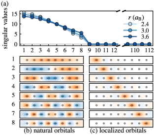
Figure A.1: Determination of the minimal basis. (a). The singular values of the stacked 1-RDMs in the molecular orbital basis of the first 400 CASSCF eigenstates for $r=2.4,3.0,3.6\,a_{\text{B}}$. (b). The natural orbitals, which are the column vectors corresponding to the eight non-zero singular values shown in (a), for $r=3.0\,a_{\text{B}}$. (c). The intrinsic atomic orbitals (IAOs) of the eight natural orbitals. These IAOs are localized in real space and used when computing the wave function descriptors.

For each interatomic separation $r$, we computed the principal components of the eigenstates’ one-body reduced density matrices (1-RDMs) in the full molecular orbital basis. Let us assume the total number of atomic orbitals which parameterize the many-body wave functions is $A$. The spin $\sigma$ 1-RDM of eigenstate $\Psi_{a}$ in molecular orbital basis $\left\{\chi_{i\sigma}\right\}$ is given by $\rho_{ij}^{\sigma}\left[\Psi_{a}\right]=\braket{\Psi_{a}}{\tilde{c}^{\dagger}_{i\sigma}\tilde{c}_{j\sigma}}{\Psi_{a}},\,\sigma=\uparrow,\,\downarrow$, where $\tilde{c}^{\dagger}_{i\sigma}$ and $\tilde{c}_{i\sigma}$ are the creation and annihilation operators of an electron in molecular orbital $\chi_{i\sigma}$, expanded in terms of the $A$ atomic orbitals. For each eigenstate, $\rho^{\sigma}$ is a matrix of size $A\times A$. We included only the first 400 many-body eigenstates, which demonstrate our method well with affordable computational cost, in the ab initio Hilbert space with ordering given by state-averaged CASSCF. Then we stacked the 1-RDMs of both spin channels for all the eigenstates in columns and obtained an $A\times(800A)$ matrix $\varrho=\big{(}\rho^{\uparrow}[\Psi_{1}],\cdots,\rho^{\uparrow}[\Psi_{400}],\rho^{\downarrow}[\Psi_{1}],\cdots,\rho^{\downarrow}[\Psi_{400}]\big{)}$, and did singular value decomposition to $\varrho$: $\varrho=U\Sigma V$. The column vectors of $U$ with non-zero singular values are the natural orbitals of the Hilbert space spanned by the first 400 eigenstates. Lastly, we computed the intrinsic atomic orbitals (IAOs) [56] of the natural orbitals. These IAOs are localized in real space and will be used for building the ab initio data set.

Appendix B Hubbard model derived using matching pursuit

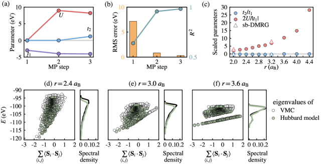
Figure B.2: (a) Parameter values for each matching pursuit (MP) step. A zero value indicates that the parameter is not yet included in the fit. (b) RMS error of the effective model and $R^{2}$ of the fit at each MP step. (c) Scaled parameter values ($t_{2}/t_{1}$ and $2U/|t_{1}|$) for each interatomic separation. For $r\geq 3.6\,a_{\text{B}}$, a $t_{1}-U$ model is chosen as the optimal model, so $t_{2}=0$. The results of the model derived using sliced-basis DMRG (sb-DMRG, see Ref. [57]) are plotted in comparison. (d-f) The VMC (multi-Slater-Jastrow wave functions with fixed Jastrow) eigenvalues and Hubbard model eigenvalues for $r=2.4,\,3.0,\,3.6\,a_{\text{B}}$, along with the comparison between their spectral densities.

In the paper, we described how the AFM Heisenberg model is detected from highly-accurate ab initio many-body calculations. We discovered that the Heisenberg model only emerges for certain interatomic separations when the ab initio eigenstates can be clustered into two sub-clusters. In fact, for hydrogen chains with AFM insulating ground states, the Hubbard model well describes all the eigenstates of interest, including both the spin and charge excitations. Fig. B.2 (a) shows the parameter values when we use the matching pursuit (MP) algorithm [58] to select the important terms in the effective Hamiltonian. MP chooses the descriptors based on their correlation with the residual of the previous fit. At MP step 1, we fit the ab initio data to a $t_{1}$ only model. Then, at MP step 2, $U$ is included in the effective Hamiltonian since it correlated the most with the residual of a $t_{1}$ mode. At MP step 3, $t_{2}$ is then included. The fit is improved as more descriptors are included in the effective Hamiltonian (see Fig. B.2 (b)), as the RMS error is reduced and $R^{2}$ is increased. In Fig. B.2 (c), we summarized the scaled fitted parameters as a function of the interatomic separation $r$ and compared them with the state-of-the-art downfolded results using sliced-basis DMRG (sb-DMRG) [57]. Our results agree with the sb-DMRG values.

In Fig. B.2 (d-f) panels, we compared the ab initio eigenvalues and the eigenvalues yielded by diagonalizing the fitted Hubbard models, along with their spectral densities. The distribution of the eigenvalues roughly agrees, while we note that there are discrepancies at the high energy. We think this is due to two possible reasons. At higher energy, the next-nearest-neighbor interaction is relevant. However, due to the lack of higher-energy ab initio data, we were not able to capture the effect of next-nearest-neighbor interaction. Also, similar to the Heisenberg model, the Hubbard model also requires renormalization using quasi-particle operators in order to accurately reproduce the ab initio properties. In Fig. 7, for the Schrieffer-Wolff transformation results, the $J$ values are computed as $J=\frac{4t_{1}^{2}}{U}$, using the $t_{1}$ and $U$ parameters obtained as above. The spectral residual of the Schrieffer-Wolff model is then evaluated with a fitted intersection $E_{0}$ value by minimizing the spectral residual.

References

- Głazek and Wilson [1993] S. D. Głazek and K. G. Wilson, Physical Review D 48, 5863 (1993).
- Głazek and Wilson [1994] S. D. Głazek and K. G. Wilson, Physical Review D 49, 4214 (1994).
- Wilson [1975] K. G. Wilson, Rev. Mod. Phys. 47, 773 (1975).
- White [1992] S. R. White, Physical Review Letters 69, 2863 (1992).
- Maier et al. [2000] T. Maier, M. Jarrell, T. Pruschke, and J. Keller, Physical Review Letters 85, 1524 (2000).
- Becca et al. [2001] F. Becca, L. Capriotti, and S. Sorella, Physical Review Letters 87, 167005 (2001).
- Sorella et al. [2002] S. Sorella, G. B. Martins, F. Becca, C. Gazza, L. Capriotti, A. Parola, and E. Dagotto, Physical Review Letters 88, 117002 (2002).
- Anisimov et al. [2002] V. I. Anisimov, M. A. Korotin, I. A. Nekrasov, Z. V. Pchelkina, and S. Sorella, Physical Review B 66, 100502(R) (2002).
- Spanu et al. [2008] L. Spanu, M. Lugas, F. Becca, and S. Sorella, Physical Review B 77, 024510 (2008).
- Ashkenazi [2011] J. Ashkenazi, Journal of Superconductivity and Novel Magnetism 24, 1281 (2011).
- Hirayama et al. [2013] M. Hirayama, T. Miyake, and M. Imada, Phys. Rev. B 87, 195144 (2013).
- Qin et al. [2020] M. Qin, C.-M. Chung, H. Shi, E. Vitali, C. Hubig, U. Schollwöck, S. R. White, and S. Zhang (Simons Collaboration on the Many-Electron Problem), Physical Review X 10, 031016 (2020).
- Jiang et al. [2021] S. Jiang, D. J. Scalapino, and S. R. White, Proceedings of the National Academy of Sciences 118, e2109978118 (2021).
- Jiang et al. [2022] S. Jiang, D. J. Scalapino, and S. R. White, Physical Review B 106, 174507 (2022).
- Witczak-Krempa et al. [2014] W. Witczak-Krempa, G. Chen, Y. B. Kim, and L. Balents, Annual Review of Condensed Matter Physics 5, 57 (2014).
- Rau et al. [2016] J. G. Rau, E. K.-H. Lee, and H.-Y. Kee, Annual Review of Condensed Matter Physics 7, 195 (2016).
- Banerjee et al. [2017] A. Banerjee, J. Yan, J. Knolle, C. A. Bridges, M. B. Stone, M. D. Lumsden, D. G. Mandrus, D. A. Tennant, R. Moessner, and S. E. Nagler, Science 356, 1055 (2017).
- Savary and Balents [2017] L. Savary and L. Balents, Reports on Progress in Physics 80, 016502 (2017).
- Zhou et al. [2017] Y. Zhou, K. Kanoda, and T.-K. Ng, Reviews of Modern Physics 89, 025003 (2017).
- Andrei and MacDonald [2020] E. Y. Andrei and A. H. MacDonald, Nature Materials 19, 1265 (2020).
- Andrei et al. [2021] E. Y. Andrei, D. K. Efetov, P. Jarillo-Herrero, A. H. MacDonald, K. F. Mak, T. Senthil, E. Tutuc, A. Yazdani, and A. F. Young, Nature Reviews Materials 6, 201 (2021).
- Huron et al. [1973] B. Huron, J. P. Malrieu, and P. Rancurel, The Journal of Chemical Physics 58, 5745 (1973).
- Ruedenberg et al. [1982] K. Ruedenberg, M. W. Schmidt, M. M. Gilbert, and S. Elbert, Chemical Physics 71, 41 (1982).
- Cimiraglia and Persico [1987] R. Cimiraglia and M. Persico, Journal of Computational Chemistry 8, 39 (1987).
- Holmes et al. [2016] A. A. Holmes, N. M. Tubman, and C. J. Umrigar, Journal of Chemical Theory and Computation 12, 3674 (2016).
- Baroni and Moroni [1999] S. Baroni and S. Moroni, Physical Review Letters 82, 4745 (1999).
- Foulkes et al. [2001] W. M. C. Foulkes, L. Mitas, R. J. Needs, and G. Rajagopal, Reviews of Modern Physics 73, 33 (2001).
- Zhang and Krakauer [2003] S. Zhang and H. Krakauer, Phys. Rev. Lett. 90, 136401 (2003).
- Booth et al. [2009] G. H. Booth, A. J. W. Thom, and A. Alavi, The Journal of Chemical Physics 131, 054106 (2009).
- White and Martin [1999] S. R. White and R. L. Martin, The Journal of Chemical Physics 110, 4127 (1999).
- Chan and Head-Gordon [2002] G. K.-L. Chan and M. Head-Gordon, The Journal of Chemical Physics 116, 10.1063/1.1449459 (2002).
- Shepherd et al. [2012] J. J. Shepherd, A. Grüneis, G. H. Booth, G. Kresse, and A. Alavi, Physical Review B 86, 035111 (2012).
- Williams et al. [2020] K. T. Williams, Y. Yao, J. Li, L. Chen, H. Shi, M. Motta, C. Niu, U. Ray, S. Guo, R. J. Anderson, J. Li, L. N. Tran, C.-N. Yeh, B. Mussard, S. Sharma, F. Bruneval, M. van Schilfgaarde, G. H. Booth, G. K.-L. Chan, S. Zhang, E. Gull, D. Zgid, A. Millis, C. J. Umrigar, and L. K. Wagner (Simons Collaboration on the Many-Electron Problem), Physical Review X 10, 011041 (2020).
- Motta et al. [2020] M. Motta, C. Genovese, F. Ma, Z.-H. Cui, R. Sawaya, G. K.-L. Chan, N. Chepiga, P. Helms, C. Jiménez-Hoyos, A. J. Millis, U. Ray, E. Ronca, H. Shi, S. Sorella, E. M. Stoudenmire, S. R. White, and S. Zhang (Simons Collaboration on the Many-Electron Problem), Physical Review X 10, 031058 (2020).
- Benali et al. [2020] A. Benali, K. Gasperich, K. D. Jordan, T. Applencourt, Y. Luo, M. C. Bennett, J. T. Krogel, L. Shulenburger, P. R. C. Kent, P.-F. Loos, A. Scemama, and M. Caffarel, The Journal of Chemical Physics 153, 184111 (2020).
- Aryasetiawan et al. [2004] F. Aryasetiawan, M. Imada, A. Georges, G. Kotliar, S. Biermann, and A. I. Lichtenstein, Physical Review B 70, 195104 (2004).
- Aryasetiawan et al. [2006] F. Aryasetiawan, K. Karlsson, O. Jepsen, and U. Schönberger, Physical Review B 74, 125106 (2006).
- Hedin [1965] L. Hedin, Physical Review 139, A796 (1965).
- Aryasetiawan and Gunnarsson [1998] F. Aryasetiawan and O. Gunnarsson, Reports on Progress in Physics 61, 237 (1998).
- Cohen et al. [2008] A. J. Cohen, P. Mori-Sánchez, and W. Yang, Science 321, 792 (2008).
- Szilva et al. [2023] A. Szilva, Y. Kvashnin, E. A. Stepanov, L. Nordström, O. Eriksson, A. I. Lichtenstein, and M. I. Katsnelson, Reviews of Modern Physics 95, 035004 (2023).
- Schrieffer and Wolff [1966] J. R. Schrieffer and P. A. Wolff, Physical Review 149, 491 (1966).
- Bravyi et al. [2011] S. Bravyi, D. P. DiVincenzo, and D. Loss, Annals of Physics 326, 2793 (2011).
- Kuzmenko et al. [2009] A. B. Kuzmenko, I. Crassee, D. van der Marel, P. Blake, and K. S. Novoselov, Phys. Rev. B 80, 165406 (2009).
- Ribeiro et al. [2009] R. M. Ribeiro, V. M. Pereira, N. M. R. Peres, P. R. Briddon, and A. H. Castro Neto, New Journal of Physics 11, 115002 (2009).
- Changlani et al. [2015] H. J. Changlani, H. Zheng, and L. K. Wagner, The Journal of Chemical Physics 143, 102814 (2015).
- Zheng et al. [2018] H. Zheng, H. J. Changlani, K. T. Williams, B. Busemeyer, and L. K. Wagner, Frontiers in Physics 6, 43 (2018).
- Chang and Wagner [2020] Y. Chang and L. K. Wagner, Physical Review Research 2, 013195 (2020).
- Dunning [1989] T. H. Dunning, The Journal of Chemical Physics 90, 1007 (1989).
- Wheeler et al. [2023] W. A. Wheeler, S. Pathak, K. G. Kleiner, S. Yuan, J. N. B. Rodrigues, C. Lorsung, K. Krongchon, Y. Chang, Y. Zhou, B. Busemeyer, K. T. Williams, A. Muñoz, C. Y. Chow, and L. K. Wagner, The Journal of Chemical Physics 158, 114801 (2023).
- Reynolds [2009] D. A. Reynolds, Encyclopedia of biometrics 741 (2009).
- Pedregosa et al. [2011] F. Pedregosa, G. Varoquaux, A. Gramfort, V. Michel, B. Thirion, O. Grisel, M. Blondel, P. Prettenhofer, R. Weiss, V. Dubourg, J. Vanderplas, A. Passos, D. Cournapeau, M. Brucher, M. Perrot, and E. Duchesnay, Journal of Machine Learning Research 12, 2825 (2011).
- Schwarz [1978] G. Schwarz, The Annals of Statistics 6, 10.1214/aos/1176344136 (1978).
- Kodinariya and Makwana [2013] T. M. Kodinariya and P. R. Makwana, International Journal 1, 90 (2013).
- Kuhn [1955] H. W. Kuhn, Naval Research Logistics Quarterly 2, 83 (1955).
- Knizia [2013] G. Knizia, Journal of Chemical Theory and Computation 9, 4834 (2013).
- Sawaya and White [2022] R. C. Sawaya and S. R. White, Physical Review B 105, 045145 (2022).
- Mallat and Zhifeng Zhang [1993] S. Mallat and Zhifeng Zhang, IEEE Transactions on Signal Processing 41, 3397 (1993).