Guaranteed quasi-error reduction of adaptive Galerkin FEM for parametric PDEs with lognormal coefficients

Abstract

Solving high-dimensional random parametric PDEs poses a challenging computational problem. It is well-known that numerical methods can greatly benefit from adaptive refinement algorithms, in particular when functional approximations in polynomials are computed as in stochastic Galerkin and stochastic collocations methods. This work investigates a residual based adaptive algorithm used to approximate the solution of the stationary diffusion equation with lognormal coefficients. It is known that the refinement procedure is reliable, but the theoretical convergence of the scheme for this class of unbounded coefficients remains a challenging open question. This paper advances the theoretical results by providing a quasi-error reduction results for the adaptive solution of the lognormal stationary diffusion problem. A computational example supports the theoretical statement.

Key words. uncertainty quantification, adaptivity, convergence, parametric PDEs, residual error estimator, lognormal diffusion

AMS subject classifications. 65N12, 65N15, 65N50, 65Y20, 68Q25

1 Introduction

In the natural sciences and engineering most modern simulation methods rely on partial differential equations (PDEs). In these applications, the simulation typically requires knowledge about many, only indirectly observable parameters such as material properties or experimental inaccuracies. Incorporating uncertainties or variations of the unknown parameters into the physical model often leads to an extremely challenging discretization complexity, also known as the “curse of dimensionality”. To mitigate the numerical obstacles and obtain a better understanding of the problems underlying structure, model order reduction techniques have been an essential area of research activity in the last decade.

One of the core ideas in this field concerns constructing a solution iteratively, increasing the complexity locally only where it is necessary. The main contribution of this work is to investigate and prove a guaranteed reduction of the quasi-error, consisting of error and error estimator, of such an adaptive algorithm, driven by a residual based error estimator, when applied to a certain class of elliptic parametric PDEs with unbounded coefficients. As a model problem, we consider the parameter dependent stationary diffusion equation

$$-\operatorname{div}_{x}\bigl{(}a(x,y)\operatorname{\nabla}_{x}u(x,y)\bigr{)} =f(x)\quad\mbox{in }D,$$ (1.1)

$$u(x,y) ~{}=0\qquad\mbox{on }\partial D,$$

on a domain $D\subset\mathbb{R}^{2}$. Here $y=(y_{1},\dots,y_{\hat{M}})\subset\mathbb{R}^{\hat{M}}$ is a high or even infinite dimensional parameter vector determining the diffusion coefficient field $a$ and hence the solution $u$ of (1.1). In particular, we consider the coefficient to be the exponential of an affine random field $\gamma$ of Gaussian variables, i.e., $a(x,y)=\exp\gamma(x,y)$, which is generally referred to as a lognormal coefficient. Several different adaptive schemes for both bounded (affine) and unbounded diffusion coefficients have been investigated in the literature [1, 2, 3, 4, 5, 6, 7, 8]. So far establishing convergence of the adaptive algorithms has only been accomplished for bounded affine diffusion coefficients [9, 10, 11, 12].

The main result of this work, Theorem 5.2, establishes that the adaptive Algorithm 1, which is based on the one described in [8], reduces the quasi-error $\operatorname{err}_{\ell}^{2}=\|\operatorname{\nabla}(u-u_{\ell})\|^{2}+\omega_{\ell}\eta_{\mathrm{det},\ell}^{2}+\omega_{\ell}\tau\eta_{\mathrm{sto},\ell}^{2}$, $\omega_{\ell},\tau>0$, in each iteration $\ell\in\mathbb{N}$, i.e.,

$$\begin{split}\operatorname{err}_{\ell+1}^{2}\leq\delta_{\ell}\operatorname{err}_{\ell}^{2},\qquad 0<\delta_{\ell}<1,\end{split}$$ (1.2)

even for an unbounded lognormal coefficient $a$. In our case the residual error estimator is composed of two contributions, namely $\eta_{\mathrm{det}}$ and $\eta_{\mathrm{sto}}$, and satisfies the reliability estimate $\|u-u_{\ell}\|^{2}\lesssim\eta_{\mathrm{det}}(u_{\ell})^{2}+\eta_{\mathrm{sto}}(u_{\ell})^{2}$ [1, 7]. We follow the proof in [9], which extends the basic strategies for deterministic finite element methods [13, 14, 15, 16, 17] to the parametric setting. Here the major difference to the bounded affine case manifests in the adapted solution spaces necessary to guarantee well-posedness of (1.1). As a consequence, establishing basic properties, such as Lipschitz continuity of $\eta_{\mathrm{det}}$ and $\eta_{\mathrm{sto}}$ or the additivity of $\eta_{\mathrm{sto}}$ with respect to the stochastic index set, becomes non-trivial.

Figure 1: Schematic overview of the ingredients required for the quasi-error reduction proof and how they are employed.

Figure 1 visualizes schematically how the newly established properties are employed to prove that Algorithm 1 reduces the quasi-error (1.2) in each iteration. We first utilize the Lipschitz continuity of $\eta_{\mathrm{det}}$ and $\eta_{\mathrm{sto}}$ as well as the continuity of $\eta_{\mathrm{det}}$ with respect to the index set to prove Lemma 5.1, which yields an upper bound of the estimator contributions depending only on quantities of the previous iteration step. Similarly, the embedding of weighted Gaussian $L^{p}$-spaces, the coercivity of the bilinear form (2.9) and the reliability of the estimator lead to a bound of the error $\|u-u_{\ell+1}\|$ by quantities depending only on level $\ell$. Refining either the spatial mesh or the stochastic space using a Dörfler marking strategy allows us to derive a quasi error reduction for the two different refinement scenarios. Here quasi additivity of $\eta_{\mathrm{sto}}$ in the index set is required to show the reduction in case $\eta_{\mathrm{sto}}$ is the dominating contribution. Finally, the involved free constants have to be chosen appropriately to ensure (1.2) holds simultaneously for both spatial and stochastic refinement for some $0<\delta<1$.

We point out that while convergence with affine coefficients can be shown [9, 10, 6], the same strong statement cannot be achieved in our setting, despite the derived quasi-error reduction in each refinement step. The crucial estimate on our analysis os commented on in Remark 5.3. Nevertheless, numerical results indicate the practical convergence of the adaptive algorithm.

The remainder of this work is structured as follows. Section 2 introduces the model problem setting, its variational formulation as well as the spatial and stochastic discretization. In Section 3, we define the residual based error estimator and introduce the algorithm that steers the adaptive refinement of the spatial mesh and the stochastic index set. Thereafter, we show some basic properties of the error estimator contributions in Section 4, which are essential to prove the main result in Section 5. Finally, we show numerical evidence to confirm the theoretical results in Section 6.

2 Parametric model problem

This section introduces the required notation for the parametric model problem (1.1). We give a short overview of the analytical setting and describe the results necessary to overcome most of the technical challenges caused by the unbounded lognormal coefficient.

2.1 Stationary diffusion with lognormal coefficient

Let $D\subset\mathbb{R}^{2}$ be a polygonal bounded Lipschitz domain representing the spatial computational area. Note that the restriction to a two dimensional spatial domain is for simplification of the problem only. All results also hold true for $D\subset\mathbb{R}^{d}$ for $d=1,2,3$, see e.g. [7] for details. For $\hat{M}\in\mathbb{N}\cup\{\infty\}$ and almost all $y\in\mathbb{R}^{\hat{M}}$, let

$$\gamma(x,y)=\sum_{m=1}^{\hat{M}}\gamma_{m}(x)y_{m}\qquad\mbox{for any }x\in D.$$ (2.1)

As we define the diffusion coefficient $a$ in (1.1) as the exponential of $\gamma$, it is important to note that the affine structure of $\gamma$ is common in applications. In a typical setting, where the randomness of the parametric problem is given through a random field with known covariance kernel, the Karhunen-Loève expansion [18] is a popular tool to decorrelate the random field into an affine sum similar to (2.1). The unbounded diffusion coefficient is now given by

$$a(x,y)=\exp(\gamma(x,y)).$$ (2.2)

Without loss of generality we restrict this work to a deterministic source term $f\in L^{2}(D)$ and homogeneous Dirichlet boundary conditions.

The unboundedness of coefficient $a$ yields an ill-posed problem and adapted function spaces have to be introduced, cf. [19, 20, 21, 22, 23]. In the following, we give a summary of the necessary concepts and refer to [7, 24] for a concise description of the underlying analysis. Let $\mathcal{X}:=H_{0}^{1}(D)$ be equipped with the norm $\|w\|_{\mathcal{X}}=\|\operatorname{\nabla}w\|_{L^{2}(D)}$, $\|w\|_{D}=\|w\|_{L^{2}(D)}$ and let $\mathcal{F}:=\{\mu\in\mathbb{N}_{0}^{\infty}\colon|\operatorname{supp}\mu|<\infty\}$ be the set of finitely supported multi-indices, where $\operatorname{supp}\mu$ denotes the set of all indices of $\mu$ different from zero. The set of admissible parameters $y\in\mathbb{R}^{\hat{M}}$ is then given by

$$\Gamma:=\{y\in\mathbb{R}^{\hat{M}}\colon\sum_{m=1}^{\hat{M}}\|\gamma_{m}\|_{L^{\infty}(D)}|y_{m}|<\infty\},$$ (2.3)

which excludes only a set of measure zero from $\mathbb{R}^{\hat{M}}$ [24]. For any $\rho\geq 0$, we set $\sigma_{m}(\rho)=\exp(\rho\|\gamma_{m}\|_{L^{\infty}(D)})\geq 1$ and define

$$\zeta_{\rho}(y):=\prod_{m=1}^{\hat{M}}\zeta_{\rho,m}(y_{m})\quad\mbox{for}\quad\zeta_{\rho,m}(y_{m}):=\frac{1}{\sigma_{m}(\rho)}\exp\Bigl{(}\bigl{(}\frac{1}{2}-\frac{1}{2\sigma_{m}(\rho)^{2}}\bigr{)}y_{m}^{2}\Bigr{)}.$$ (2.4)

Since $\zeta_{\rho,m}$ is the Radon-Nikodym derivative of $\mathcal{N}(0,\sigma_{m}(\rho)^{2})$ with respect to the standard Gaussian measure, we can define the probability density function of $\mathcal{N}(0,\sigma_{m}(\rho)^{2})$ via

$$\pi_{\rho,m}(y_{m})=\zeta_{\rho,m}(y_{m})\frac{1}{\sqrt{2\pi}}\exp(-\frac{1}{2}y_{m}^{2}).$$ (2.5)

Note that $\pi_{0,m}$ is the density of the standard Gaussian measure itself, since $\zeta_{0,m}\equiv 1$. With this, we define the weighted product measure $\pi_{\rho}(y):=\prod_{m=1}^{\hat{M}}\pi_{\rho,m}(y_{m})$. Since we assume $y_{m}\sim\mathcal{N}(0,\sigma_{m}(\rho)^{2})$ for some $\rho>0$, we refer to $a$ as a lognormal coefficient field.

For any $\vartheta\in[0,1]$ and $\rho>0$, define the bilinear form for all $w,v\in L^{2}(\Gamma,\pi_{\vartheta\rho};\mathcal{X})$ by

$$B(w,v):=B_{\vartheta\rho}(w,v):=\int_{\Gamma}\int_{D}a(x,y)\operatorname{\nabla}w(x,y)\cdot\operatorname{\nabla}v(x,y)\,\mathrm{d}x\,\mathrm{d}\pi_{\vartheta\rho}(y)$$ (2.6)

and denote by $\|w\|_{B}=B(w,w)^{1/2}$ the energy norm induced by $B$. Additionally, let $\|w\|_{\pi_{\vartheta\rho},D}=\|w\|_{L^{2}(\Gamma,\pi_{\vartheta\rho};L^{2}(D))}$. The variational form of (1.1) then reads: Find $u\in\mathcal{V}$ such that

$$B(u,v)=F(v)\quad\mbox{for all }v\in\mathcal{V},$$ (2.7)

where $F(v)=\int_{\Gamma}\int_{D}f(x)v(x,y)\,\mathrm{d}x\,\mathrm{d}\pi_{\vartheta\rho}(y)$ and

$$\mathcal{V}:=\{w\colon\Gamma\to\mathcal{X}\mbox{ measurable with }B_{\vartheta\rho}(w,w)<\infty\}.$$

Remark 2.1.

With this problem adapted function space, it follows by [24, Proposition 2.43] that

$$L^{2}(\Gamma,\pi_{\rho};\mathcal{X})\subset\mathcal{V}\subset L^{2}(\Gamma,\pi_{0};\mathcal{X})$$

are continuous embeddings for any $0<\vartheta<1$. Thus, the bilinear form $B_{\vartheta\rho}$ is $\mathcal{V}$–elliptic and bounded in the sense that

$$|B_{\vartheta\rho}(w,v)| \leq\hat{c}_{\vartheta\rho}\,\|\operatorname{\nabla}w\|_{\pi_{\rho},D}\,\|\operatorname{\nabla}v\|_{\pi_{\rho},D} \mbox{for all }w,v\in L^{2}(\Gamma,\pi_{\rho};\mathcal{X}),$$ (2.8)

$$B_{\vartheta\rho}(w,w) \geq\check{c}_{\vartheta\rho}\|\operatorname{\nabla}w\|_{\pi_{0},D}^{2} \mbox{for all }w\in L^{2}(\Gamma,\pi_{0};\mathcal{X}),$$ (2.9)

for some $\hat{c}_{\vartheta\rho},\check{c}_{\vartheta\rho}>0$, which implies the well-posedness of (2.7).

2.2 Discretization

Since the spatial domain $D$ has a polygonal boudary, we assume a shape regular triangulation $\mathcal{T}$ that represents $D$ exactly. We denote by $\mathcal{E}$ the set of edges of $\mathcal{T}$ and let $\partial T=\{E\in\mathcal{E}\colon E\cap\bar{T}\neq\emptyset\}$ for any triangle $T\in\mathcal{T}$. For any $E\in\mathcal{E}$ denote by $h_{E}=|E|$ the length of $E$ and let $h_{T}=\max_{E\in\partial T}h_{E}$ denote the diameter of any $T\in\mathcal{T}$.

For the spatial discretization, consider the conforming Lagrange finite element space of order $p$

$$\mathcal{X}_{p}(\mathcal{T})=P_{p}(\mathcal{T})\cap C(\bar{\mathcal{T}})=\operatorname{span}\{\varphi_{j}\}_{j=1}^{J},$$ (2.10)

where $P_{p}(\mathcal{T})$ denotes the space of element-wise polynomials of order $p$. Here, $J\in\mathbb{N}$ denotes the dimension of the finite element space. Define the normal jump of a function $\xi\in H^{1}(D;\mathbb{R}^{2})$ over the edge $E=\bar{T}\cap\bar{T^{\prime}}$ by $\llbracket\xi\rrbracket_{E}=(\xi|_{T}-\xi|_{T^{\prime}})\cdot n_{E}$ for the edge normal vector $n_{E}=n_{T}=-n_{T^{\prime}}$ of $E$. Since the direction of the normal $n_{E}$ depends on the enumeration of the neighbouring triangles, we assume an arbitrary but fixed choice of the sign of $n_{E}$ for each $E\in\mathcal{E}$.

By $\{P^{m}_{k}\}_{k=0}^{\infty}$ we denote a set of orthogonal and normalized polynomials in $L^{2}(\Gamma,\pi_{\vartheta\rho,m})$. This defines a tensorized orthonormal product basis $\{P_{\mu}\}_{\mu\in\mathcal{F}}$ of $L^{2}(\Gamma,\pi_{\vartheta\rho})$ by $P_{\mu}(y):=\prod_{m=1}^{\hat{M}}P_{\mu_{m}}^{m}(y_{m})=\prod_{m\in\operatorname{supp}\mu}P_{\mu_{m}}^{m}(y_{m})$. Due to the weighted $L^{2}$ spaces of our functional setting, the basis $\{P_{\mu}\}$ consists of scaled Hermite polynomials, see [24, 8]. Note that the use of global polynomials is justified by the high (holomorphic) regularity of the solution of (1.1) with respect to the stochastic variables [25, 26, 20]. For any $\alpha,\beta,\mu\in\mathbb{N}_{0}^{\hat{M}}$ we define the triple product

$$\tau_{\alpha\beta\mu}:=\prod_{m=1}^{\hat{M}}\tau_{\alpha_{m}\beta_{m}\mu_{m}}^{m}\qquad\mbox{for}\qquad\tau_{\alpha_{m}\beta_{m}\mu_{m}}^{m}:=\int_{\Gamma}P_{\alpha_{m}}^{m}P_{\beta_{m}}^{m}P_{\mu_{m}}^{m}\,\mathrm{d}\pi_{\vartheta\rho,m}(y)$$ (2.11)

and note that $\tau_{ijk}^{m}=0$ if $i+j+k$ is odd or if $\max\{i,j,k\}>(i+j+k)/2$. For more analytical properties of the scaled Hermite polynomials we refer to [7, 8].

For any $j\in\mathbb{N}_{0}$ and $k\in\mathbb{N}$, let $[j\operatorname{:}k]:=\{j,\dots,k-1\}$, where $[j\operatorname{:}k]:=\{0\}$ if $j\geq k$ and $[k]:=[0\operatorname{:}k-1]$. Define the full tensor index set $\Lambda_{d}$ for any $d\in\mathbb{N}^{\hat{M}}$ by

$$\Lambda_{d}:=[d_{1}]\times\dots[d_{\hat{M}}]\times[1]\times\dots\subset\mathcal{F}.$$ (2.12)

Given two full tensor sets $\Lambda_{d},\Lambda_{\hat{d}}$ with $d,\hat{d}\in\mathbb{N}^{\hat{M}}$, we define the sum of the two sets by $\Lambda_{d}+\Lambda_{\hat{d}}=\Lambda_{d+\hat{d}-1}$ and refer to $\partial\Lambda_{d}=\partial_{\hat{d}}\Lambda_{d}=\Lambda_{d+\hat{d}-1}\setminus\Lambda_{d}$ as the boundary of $\Lambda_{d}$ with respect to $\Lambda_{\hat{d}}$. Note that we will implicitly assume $d=(d_{1},\dots,d_{M},1,\dots,1)\in\mathbb{N}^{\hat{M}}$ for any $d\in\mathbb{N}^{M}$ with $M<\hat{M}$ to ensure compatibility of dimensions.

Given these sets, we define the fully discrete approximation space by

$$\mathcal{V}_{N}:=\mathcal{V}_{N}(\Lambda_{d};\mathcal{T},p):=\Bigl{\{}w_{N}(x,y)=\sum_{j=1}^{J}\sum_{\mu\in\Lambda_{d}}\boldsymbol{w_{N}}[j,\mu]\varphi_{j}(x)P_{\mu}(y)\mbox{ with }\boldsymbol{w_{N}}\in\mathbb{R}^{J\times d}\Bigr{\}}\subset\mathcal{V}.$$ (2.13)

We refer to $\boldsymbol{w_{N}}$ as the coefficient tensor of $w_{N}$ with respect to the bases $\{\varphi_{j}\}$ and $\{P_{\mu}\}$. With this the Galerkin projection $u_{N}\in\mathcal{V}_{N}$ of the solution $u$ of (2.7) is determined uniquely by

$$B(u_{N},v_{N})=F(v_{N})\qquad\mbox{for all }v_{N}\in\mathcal{V}_{N}.$$ (2.14)

3 Error estimator and adaptive algorithm

In this section a reliable residual based error estimator for the Galerkin solution $u_{N}\in\mathcal{V}_{N}$ is introduced. Moreover, an algorithm for the adaptive refinement of the spatial and stochastic approximation spaces is described. The estimator we define is based on the one presented in [7] and we refer to [1, 9, 7] for details on the underlying analysis.

3.1 A posteriori error estimator

In the following, let $p\in\mathbb{N}$ be some fixed FE polynomial degree, $d\in\mathbb{N}^{M}$ and $\hat{d}\in\mathbb{N}^{\hat{M}}$ for $M\leq\hat{M}\in\mathbb{N}$. Furthermore, assume that we have access to an approximation $a_{N}\in\mathcal{V}_{N}(\Lambda_{\hat{d}};\mathcal{T},p)$ of (2.2) of the form

$$a(x,y)\approx a_{N}(x,y)=\sum_{j=1}^{J}\sum_{\hat{\mu}\in\Lambda_{\hat{d}}}\boldsymbol{a_{N}}[j,\hat{\mu}]\varphi_{j}(x)P_{\hat{\mu}}(y)$$ (3.1)

for any triangulation $\mathcal{T}$. In order to avoid an obfuscation of the analysis, we assume the approximation error to be negligible with respect to the overall error we would like to achieve. Then, for any $w\in\mathcal{V}$, consider the residual $\mathcal{R}(w)\in\mathcal{V}^{*}=L^{2}(\Gamma,\pi_{\vartheta\rho};\mathcal{X}^{*})$ of (2.7) for $a_{N}$ instead of $a$, given implicitly for all $v\in\mathcal{V}$ by

$$\langle\mathcal{R}(w),v\rangle_{V^{*},V}=\int_{\Gamma}\int_{D}f(x)v(x,y)-a_{N}(x,y)\operatorname{\nabla}w(x,y)\cdot\operatorname{\nabla}v(x,y)\,\mathrm{d}x\,\mathrm{d}\pi_{\vartheta\rho}(y).$$ (3.2)

Similarily, we consider the bilinear form (2.6) with $a_{N}$ instead of $a$ in the following.

Remark 3.1.

The residual associated to (2.7) can be split into a term containing $\mathcal{R}(w)$ and a term describing the approximation error of the diffusion coefficient

$$\langle f+\operatorname{div}(a\operatorname{\nabla}w),v\rangle_{\mathcal{V}^{*},V}=\langle\mathcal{R}(w),v\rangle_{\mathcal{V}^{*},V}+\int_{\Gamma}\int_{D}(a-a_{N})\operatorname{\nabla}w\cdot\operatorname{\nabla}v\,\mathrm{d}x\,\mathrm{d}\pi_{\vartheta\rho}(y),$$ (3.3)

which implies that the task of finding $a_{N}$ to approximate (2.2) can be considered separately. Since there exist several approaches to compute such an approximation [27, 28, 7, 29] and [29] even provides a computable a posteriori bound of the approximation error for any $a_{N}\in\mathcal{V}_{N}(\Lambda_{\hat{d}};\mathcal{T},p)$, we assume that the second term of (3.3) is negligible and restrict ourselves to (3.2). We also need to assume that (2.8)– (2.9) still hold when using $a_{N}$ instead of $a$, possibly with different constants $\hat{c}_{\vartheta\rho}$ and $\check{c}_{\vartheta\rho}$. Note that the solution error incurred by approximating $u$ by $u_{N}$ is bounded by the Strang lemma, see e.g. [30, Chap. 3-§1].

For any $w_{N}\in\mathcal{V}_{N}$ we define $r(w_{N}):=a_{N}\operatorname{\nabla}w_{N}$ and note that by [7, Lemma 3.1]

$$r(w_{N})=\sum_{\mu\in\Lambda_{d+\hat{d}-1}}r_{\mu}(w_{N})P_{\mu}\quad\mbox{for}\quad r_{\mu}(w_{N})=\sum_{j,k=1}^{J}\sum_{\alpha\in\Lambda_{d}}\sum_{\hat{\alpha}\in\Lambda_{\hat{d}}}\boldsymbol{a_{N}}[k,\hat{\alpha}]\boldsymbol{w_{N}}[j,\alpha]\tau_{\alpha\hat{\alpha}\mu}\varphi_{k}\operatorname{\nabla}\varphi_{j}$$ (3.4)

has support on $\Lambda_{d+\hat{d}-1}$ due to the properties of the triple product $\tau_{\alpha\hat{\alpha}\mu}$. With this we introduce the deterministic estimator contribution

$$\eta_{\mathrm{det}}(w_{N},\mathcal{T},\Lambda_{d})^{2}:=\sum_{T\in\mathcal{T}}\Bigl{(}\eta_{\mathrm{det},T}(w_{N},\Lambda_{d})^{2}+\eta_{\mathrm{det},\partial T}(w_{N},\Lambda_{d})^{2}\Bigr{)}$$ (3.5)

for volume and jump contributions given by

$$\eta_{\mathrm{det},T}(w_{N},\Lambda_{d}) :=h_{T}\|\sum_{\mu\in\Lambda_{d}}\bigl{(}f\delta_{\mu 0}-\operatorname{div}r_{\mu}(w_{N})\bigr{)}P_{\mu}\,\zeta_{\vartheta\rho}\|_{\pi_{0},T},$$ (3.6)

$$\eta_{\mathrm{det},\partial T}(w_{N},\Lambda_{d}) :=h_{T}^{1/2}\|\sum_{\mu\in\Lambda_{d}}\llbracket r_{\mu}(w_{N})\rrbracket_{\partial T}P_{\mu}\,\zeta_{\vartheta\rho}\|_{\pi_{0},\partial T},$$ (3.7)

where $\delta_{\mu\hat{\mu}}$ denotes the (multiindex) Kronecker delta. In a similar fashion we define the stochastic estimator contribution by

$$\eta_{\mathrm{sto}}(w_{N},\Delta):=\|\sum_{\mu\in\Delta}r_{\mu}(w_{N})P_{\mu}\zeta_{\vartheta\rho}\|_{\pi_{0},D}\qquad\mbox{for any }\qquad\Delta\subseteq\partial\Lambda_{d}.$$ (3.8)

Let the overall error estimator for any $w_{N}\in\mathcal{V}_{N}$ and (heuristically chosen) equilibration constant $c_{\mathrm{ref}}>0$ be given by

$$\eta(w_{N})^{2}=\eta_{\mathrm{det}}(w_{N},\mathcal{T},\Lambda_{d})^{2}+c_{\mathrm{ref}}^{2}\eta_{\mathrm{sto}}(w_{N},\partial\Lambda_{d})^{2}.$$ (3.9)

Then [7] yields the following reliability bound.

Theorem 3.2 (reliability).

Let $u$ be the solution of (2.7) and let $u_{N}\in\mathcal{V}_{N}$ be the Galerkin solution of (2.14). There exists a constant $c_{\mathrm{rel}}>0$ depending only on the constant in (2.9) and the shape regularity of $\mathcal{T}$ such that

$$\|u-u_{N}\|_{B}\leq c_{\mathrm{rel}}\,\eta(u_{N}).$$

Remark 3.3.

The estimator considered in [7] is not the same as (3.9) for two reasons. First, (3.7) has a different ordering, which implies that (3.5) is equivalent to the deterministic estimator contribution in [7] with a constant depending only on the shape regularity of $\mathcal{T}$. Second, we neglect error contributions introduced by the low-rank compression and the inexact iterative solver of the Galerkin solution $u_{N}$ of (2.14). This is motivated by promising experimental results in recent works [31, 32, 33], where it is shown numerically that these errors can in principle be controlled. Hence, we assume that the Galerkin solution $u_{N}$ is computable and focus on showing the reduction of the quasi-error through the adaptive algorithm in our setting.

3.2 Adaptive algorithm

Given a fixed FE polynomial degree $p\in\mathbb{N}_{0}$, an initial triangulation $\mathcal{T}$ and initial stochastic dimensions $d\in\mathbb{N}^{M}$, Algorithm 1 relies on a classical loop of Solve, Estimate, Mark and Refine to generate approximative solutions $u_{\ell}$ of (1.1). According to Remark 3.1, we assume $\hat{d}\in\mathbb{N}^{\hat{M}}$ sufficiently large such that the approximation error of the discretized diffusion coefficient (3.1) is negligible in each iteration of Algorithm 1. As $\hat{d}$ remains unchanged during the algorithm, we abbreviate $\partial\Lambda_{d}=\partial_{\hat{d}}\Lambda_{d}$ in the following.

Input: mesh $\mathcal{T}$; FE polynomial degree $p$; stochastic dimensions $d$; Dörfler thresholds $0<\theta_{\mathrm{det}},\theta_{\mathrm{sto}}\leq 1$; maximum number of iterations $L$; look ahead $q\in\mathbb{N}^{\hat{M}}$

1 set $\mathcal{T}_{1}=\mathcal{T}$, $\Lambda_{d_{1}}=\Lambda_{d}$;

2 for $\ell=1,2,\dots$ do

3      Solve

4            compute solution $u_{\ell}\in\mathcal{V}_{N}(\Lambda_{d_{\ell}};\mathcal{T}_{\ell},p)$ of (2.14);

5      

6      Estimate

7            compute $\eta_{\mathrm{det},\ell}(u_{\ell},\mathcal{T}_{\ell},\Lambda_{d_{\ell}})$ as in (3.5);

8             compute $\eta_{\mathrm{sto},\ell}(u_{\ell},\partial\Lambda_{d_{\ell}})$ as in (3.8);

9            

10      

11      if $\ell\geq L$: break

12      

13      Mark

14            if $\eta_{\mathrm{det},\ell}(u_{\ell},\mathcal{T}_{\ell},\Lambda_{d_{\ell}})\geq c_{\mathrm{ref}}\,\eta_{\mathrm{sto},\ell}(u_{\ell},\partial\Lambda_{d_{\ell}})$ then

15                  set $\Delta_{\ell}=\emptyset$ and choose minimal set $\mathcal{M}_{\ell}\subseteq\mathcal{T}_{\ell}$ such that $\eta_{\mathrm{det},\ell}(u_{\ell},\mathcal{M}_{\ell},\Lambda_{d_{\ell}})\geq\theta_{\mathrm{det}}\,\eta_{\mathrm{det},\ell}(u_{\ell},\mathcal{T}_{\ell},\Lambda_{d_{\ell}})$;

16            else

17                  choose minimal set $\mathcal{M}\subseteq\{1,\dots,\hat{M}\}$ such that $\sum_{m\in\mathcal{M}}\eta_{\mathrm{sto},\ell}(u_{\ell},\Delta_{\ell,m,q_{m}})\geq\theta_{\mathrm{sto}}\,\eta_{\mathrm{sto},\ell}(u_{\ell},\partial\Lambda_{d_{\ell}})$;

18                   set $\mathcal{M}_{\ell}=\emptyset$ and $\Delta_{\ell}=\bigcup_{m\in\mathcal{M}}\Delta_{\ell,m,q_{m}}$;

19            

20      

21      Refine

22            $\mathcal{T}_{\ell+1}\leftarrow\mathrm{\bf bisect}(\mathcal{T}_{\ell},\mathcal{M}_{\ell})$;

23             $\Lambda_{d_{l+1}}\leftarrow\Lambda_{d_{\ell}}\cup\Delta_{\ell}$;

24      

Algorithm 1 Adaptive refinement scheme

In each iteration $\ell$ of the loop, we compute the Galerkin solution $u_{\ell}$ of (2.14) (Solve) and the estimator contributions (3.5) and (3.8) (Estimate). During the Mark step, we employ a conditional Dörfler marking strategy based on the dominating estimator contribution to determine how to refine $\mathcal{T}_{\ell}$ and $\Lambda_{d_{\ell}}$. If $\eta_{\mathrm{det},\ell}(u_{\ell},\mathcal{T}_{\ell},\Lambda_{d_{\ell}})$ dominates we set the marked stochastic set $\Delta_{\ell}=\emptyset$ and employ a Dörfler marking strategy to the mesh $\mathcal{T}_{\ell}$, where we use the Dörfler threshold $\theta_{\mathrm{det}}$. For the refinement of the spatial mesh $\mathcal{T}_{\ell}$ we use newest vertex bisection [17] on all marked elements $T\in\mathcal{M}_{\ell}$, which is denoted by ${\bf bisect}(\mathcal{T}_{\ell},\mathcal{M}_{\ell})$ in Algorithm 1. If, on the other hand, $c_{\mathrm{ref}}\,\eta_{\mathrm{sto},\ell}(u_{\ell},\partial\Lambda_{d_{\ell}})$ dominates, where $c_{\mathrm{ref}}$ is the equilibration constant in (3.9), we set the marked triangles to $\mathcal{M}_{\ell}=\emptyset$ and employ the Dörfler marking with threshold $\theta_{\mathrm{sto}}$ to {$\Delta_{\ell,m,q_{m}}\}_{m=1}^{\hat{M}}$. The index sets $\Delta_{\ell,m,q_{m}}$ are given for each $m=1,\dots,\hat{M}$ by

$$\Delta_{\ell,m,q_{m}}=\bigotimes_{j=1}^{m-1}[d_{j}]\ \otimes\ [d_{m}:d_{m}+q_{m}]\ \otimes\ \bigotimes_{j=m+1}^{\hat{M}}[d_{j}]\qquad\mbox{for }q_{m}\in[1\operatorname{:}\hat{d}_{m}-1].$$ (3.10)

Algorithm 1 iterates through the Solve, Estimate, Mark and Refine routines until the maximal number of loops is reached. Note that specifying the maximum number of iterations a priori in Algorithm 1 is impractical for most applications and done here only for simplification. More reasonable stopping criteria such as specifying a target threshold for the total error estimator or limiting the maximum of allowed degrees of freedom could be applied as well.

4 Estimator Properties

In this section we establishes some fundamental properties of the estimator contributions, which are required to prove the quasi-error reduction of Algorithm 1 for the unbounded lognormal diffusion coefficient (2.2). The proof follows [9] and is based on the continuity of the estimators. As a preparation, we first establish how $\zeta_{\rho}^{\alpha}\pi_{0}$ behaves for different exponents $\alpha\geq 0$.

Lemma 4.1 (embedding of weighted $L^{p}$-spaces).

Let $\alpha\geq 0$ and

$$0\leq\rho\leq\rho_{\alpha}=\begin{cases}1&\mbox{if }\alpha\leq 1,\\ \min\Bigl{\{}1,\frac{\ln(\alpha(\alpha-1)^{-1})}{2\hat{\gamma}}\Bigr{\}}&\mbox{if }\alpha>1,\end{cases}$$

where $\hat{\gamma}$ is an upper bound for (2.1), i.e., $\|\gamma_{m}\|_{L^{\infty}(D)}\leq\hat{\gamma}$ for all $m=0,\dots,\hat{M}$. Then there exists a constant $c_{\alpha}>0$ such that $\pi_{\rho,\alpha}=c_{\alpha}\zeta_{\rho}^{\alpha}\pi_{0}$ is the probability density function of a centered Gaussian distribution. Moreover, for any $0\leq\alpha\leq\beta$ and $\rho\leq\rho_{\beta}$, it holds

$$L^{p}(\Gamma,\pi_{\rho,\beta})\subset L^{p}(\Gamma,\pi_{\rho,\alpha})\qquad\mbox{for any }p\in[1,\infty).$$

Proof.

Note that for any $\alpha>0$ and $\sigma_{\alpha,m}(\rho)=\sigma_{m}(\rho)\bigl{(}\alpha+(1-\alpha)\sigma_{m}(\rho)^{2}\bigr{)}^{-1/2}$ it holds

$$\begin{split}\zeta_{\rho,m}(y_{m})^{\alpha}\pi_{0,m}(y_{m})&=\frac{1}{\sqrt{2\pi}\sigma_{m}(\rho)^{\alpha}}\exp\Bigl{(}-\frac{y_{m}^{2}}{2\sigma_{\alpha,m}(\rho)^{2}}\Bigr{)}.\end{split}$$

Defining the normalization constant

$$c_{\alpha,m}(\rho):=\sigma_{m}(\rho)^{\alpha-1}\sqrt{\alpha+(1-\alpha)\sigma_{m}(\rho)^{2}}=\sigma_{m}(\rho)^{\alpha}\sigma_{\alpha,m}(\rho)^{-1}$$

then yields that $\pi_{\rho,\alpha,m}=c_{\alpha,m}(\rho)\zeta_{\rho,m}^{\alpha}\pi_{0,m}$ is the probability density function of a univariate centered Gaussian distribution with variance $\sigma_{\alpha,m}(\rho)^{2}$. Since $\sigma_{m}(\rho)=\exp(\rho\|\gamma_{m}\|_{L^{\infty}(D)})$, we need

$$0<\rho<\begin{cases}1&\mbox{if }\alpha\leq 1,\\ \min\Bigl{\{}1,\frac{\ln(\alpha(\alpha-1)^{-1})}{2\|\gamma_{m}\|_{L^{\infty}(D)}}\Bigr{\}}&\mbox{if }\alpha>1,\end{cases}$$

to ensure that $\pi_{\rho,\alpha,m}$ is integrable with respect to the standard Lebesgue measure. As a consequence and by the definition of $\hat{\gamma}$, $\rho\leq\rho_{\alpha}$ ensures integrability of $\pi_{\rho,\alpha}=\prod_{m=1}^{\hat{M}}\pi_{\rho,\alpha,m}$. It is easy to see that for any $0<\alpha<\beta\in\mathbb{R}$ and $w\in L^{p}(\Gamma,\pi_{\rho,\beta})$,

$$\|w\|_{L^{p}(\Gamma,\pi_{\rho,\alpha})}\leq c\,\|\zeta_{\rho}^{\alpha-\beta}\|_{L^{\infty}(\Gamma)}\|w\|_{L^{p}(\Gamma,\pi_{\rho,\beta})}\quad\text{with}\quad c=\prod_{m=1}^{\hat{M}}\frac{c_{\alpha,m}(\rho)}{c_{\beta,m}(\rho)}.$$

Moreover, $|\zeta_{\rho,m}^{\alpha-\beta}|\leq\sigma_{m}(\rho)^{\beta-\alpha}<\infty$, which implies

$$\|\zeta_{\rho}^{\alpha-\beta}\|_{L^{\infty}(\Gamma)}=\prod_{m=1}^{\hat{M}}\sigma_{m}(\rho)^{\beta-\alpha}<\infty.$$

Consequently, $L^{p}(\Gamma,\pi_{\rho,\beta})\subset L^{p}(\Gamma,\pi_{\rho,\alpha})$ for all $1\leq p\in\mathbb{R}$. ∎

To prove the Lipschitz continuity of $\eta_{\mathrm{det}}$ and $\eta_{\mathrm{sto}}$ later in this section, we also require the following observation.

Corollary 4.2.

Let $w$ be a polynomial, $\alpha\geq 0$ and $\rho\leq\rho_{\alpha}$ as in Lemma 4.1. Then it holds

$$\|w\zeta_{\rho}^{\alpha}\|_{L^{p}(\Gamma,\pi_{0})}<\infty.$$

Proof.

By Lemma 4.1 there exists a constant $c>0$ such that $\|w\zeta_{\rho}^{\alpha}\|_{L^{p}(\Gamma,\pi_{0})}^{p}=c\|w\|_{L^{p}(\Gamma,\pi_{\rho,p\alpha})}^{p}$. Since $w$ is a polynomial and $\pi_{\rho,p\alpha}$ decays exponentially, $\|w\|_{L^{p}(\Gamma,\pi_{\rho,p\alpha})}<\infty$. ∎

4.1 Deterministic estimator contribution

In the following, we show that the deterministic estimator contribution (3.5) satisfies some continuity conditions.

Theorem 4.3 (Lipschitz continuity of $\eta_{\mathrm{det,T}}$ in the first component).

For any $v_{N},w_{N}\in\mathcal{V}_{N}=\mathcal{V}_{N}(\Lambda_{d};\mathcal{T},p)$ and $T\in\mathcal{T}$ there exists a constant $c_{\mathrm{det}}>0$ depending only on the active set $\Lambda_{d}$, such that

$$|\eta_{\mathrm{det},T}(v_{N},\Lambda_{d})-\eta_{\mathrm{det},T}(w_{N},\Lambda_{d})|\leq c_{\mathrm{det}}\|\operatorname{\nabla}(v_{N}-w_{N})\|_{\pi_{\vartheta\rho},T}.$$

Proof.

For any $\mu\in\Lambda_{d}$ consider the expansion $P_{\mu}\zeta_{\vartheta\rho}=\sum_{\nu\in\mathbb{N}_{0}^{\hat{M}}}z_{\mu,\nu}H_{\nu}$ where $\{H_{\nu}\}_{\nu\in\mathbb{N}_{0}^{\hat{M}}}$ is an orthonormal basis in $L^{2}(\Gamma,\pi_{0})$. Additionally, define the estimator components

$$\eta_{\mathrm{det},T,\nu}(v_{N},\Lambda_{d}) :=h_{T}\Bigl{\|}\sum_{\mu\in\Lambda_{d}}\bigl{(}f\delta_{\mu 0}+\operatorname{div}r_{\mu}(v_{N})\bigr{)}z_{\mu,\nu}\Bigr{\|}_{T},$$ (4.1)

$$\eta_{\mathrm{det},\partial T,\nu}(v_{N},\Lambda_{d}) :=h_{T}^{1/2}\Bigl{\|}\sum_{\mu\in\Lambda_{d}}\llbracket r_{\mu}(v_{N})\rrbracket_{\partial T}z_{\mu,\nu}\Bigr{\|}_{\partial T\cap D}.$$ (4.2)

With the inverse estimate $\|\operatorname{div}\xi_{N}\|_{T}\leq c_{\mathrm{inv}}h_{T}^{-1}\|\xi_{N}\|_{T}$ for any $\xi_{N}\in\operatorname{\nabla}\mathcal{V}_{N}=\{\operatorname{\nabla}v_{N}\colon v_{N}\in\mathcal{V}_{N}\}$ it holds

$$\begin{split}&|\eta_{\mathrm{det},T,\nu}(v_{N},\Lambda_{d})-\eta_{\mathrm{det},T,\nu}(w_{N},\Lambda_{d})|\\ &\qquad\leq h_{T}\|\operatorname{div}\bigl{(}\sum_{\mu\in\Lambda_{d}}r_{\mu}(v_{N}-w_{N})z_{\mu,\nu}\bigr{)}\|_{T}\\ &\qquad\leq c_{\mathrm{inv}}\|\sum_{\mu\in\Lambda_{d}}r_{\mu}(v_{N}-w_{N})z_{\mu,\nu}\|_{T}\\ &\qquad=c_{\mathrm{inv}}\|\sum_{\mu\in\Lambda_{d}}\sum_{\alpha\in\Lambda_{\hat{d}}}\sum_{\beta\in\Lambda_{d}}a_{\alpha}\operatorname{\nabla}(v_{N}-w_{N})_{\beta}\tau_{\alpha\beta\mu}z_{\mu,\nu}\|_{T}\\ &\qquad\leq\sum_{\mu\in\Lambda_{d}}\sum_{\alpha\in\Lambda_{d+\tilde{d}-1}}\sum_{\beta\in\Lambda_{d}}c_{\mathrm{inv}}\|a_{\alpha}\|_{L^{\infty}(D)}\|\operatorname{\nabla}(v_{N}-w_{N})_{\beta}\|_{T}|\tau_{\alpha\beta\mu}z_{\mu,\nu}|,\end{split}$$

where $\tilde{d}$ is the component wise minimum of $d$ and $\hat{d}$ and $a_{\alpha}=\sum_{k=1}^{J}\boldsymbol{a}_{N}[k,\alpha]\varphi_{k}\in\mathcal{X}_{p}(\mathcal{T})$. By the same argument and the inverse estimate $\|\operatorname{\nabla}\xi_{N}\cdot n_{T}\|_{\partial T\cap D}\leq c_{\mathrm{inv}}h_{T}^{-1/2}\|\operatorname{\nabla}\xi_{N}\|_{T}$ for any $\xi_{N}\in\mathcal{V}_{N}$, with the outer unit normal vector $n_{T}$ of $T$, we derive the bound

$$\begin{split}&|\eta_{\mathrm{det},\partial T,\nu}(v_{N},\Lambda_{d})-\eta_{\mathrm{det},\partial T,\nu}(w_{N},\Lambda_{d})|\\ &\qquad\leq\sum_{\mu\in\Lambda_{d}}\sum_{\alpha\in\Lambda_{d+\tilde{d}-1}}\sum_{\beta\in\Lambda_{d}}2c_{\mathrm{inv}}\|a_{\alpha}\|_{L^{\infty}(D)}\|\operatorname{\nabla}(v_{N}-w_{N})_{\beta}\|_{T}|\tau_{\alpha\beta\mu}z_{\mu,\nu}|.\end{split}$$

Let $s_{T,\nu}:=\eta_{\mathrm{det},T,\nu}(v_{N},\Lambda_{d})+\eta_{\mathrm{det},T,\nu}(w_{N},\Lambda_{d})$ and $s_{\partial T,\nu}=\eta_{\mathrm{det},\partial T,\nu}(v_{N},\Lambda_{d})+\eta_{\mathrm{det},\partial T,\nu}(w_{N},\Lambda_{d})$. The previous two estimates and the third binomial formula then yield

$$\begin{split}&|\eta_{\mathrm{det},T}(v_{N},\Lambda_{d})^{2}-\eta_{\mathrm{det},T}(w_{N},\Lambda_{d})^{2}|\\ &\qquad\leq\sum_{\nu\in\mathbb{N}_{0}^{\hat{M}}}|\eta_{\mathrm{det},T,\nu}(v_{N},\Lambda_{d})-\eta_{\mathrm{det},T,\nu}(w_{N},\Lambda_{d})|\,s_{T,\nu}\\ &\qquad\qquad+\sum_{\nu\in\mathbb{N}_{0}^{\hat{M}}}|\eta_{\mathrm{det},\partial T,\nu}(v_{N},\Lambda_{d})-\eta_{\mathrm{det},\partial T,\nu}(w_{N},\Lambda_{d})|\,s_{\partial T,\nu}\\ &\qquad\leq\sum_{\beta\in\Lambda_{d}}\|\operatorname{\nabla}(v_{N}-w_{N})_{\beta}\|_{T}\,S_{\beta}\end{split}$$

for

$$S_{\beta}:=\sum_{\alpha\in\Lambda_{d+\tilde{d}-1}}\sum_{\mu\in\Lambda_{d}}\sum_{\nu\in\mathbb{N}_{0}^{\hat{M}}}c_{\mathrm{inv}}\|a_{\alpha}\|_{L^{\infty}(D)}(s_{T,\nu}+2s_{\partial T,\nu})|\tau_{\alpha\beta\mu}z_{\mu,\nu}|.$$

We now define the constant

$$c(\Lambda_{d})^{2}:=\sum_{\beta\in\Lambda_{d}}\sum_{\nu\in\mathbb{N}_{0}^{\hat{M}}}\Bigl{(}\sum_{\mu\in\Lambda_{d}}\sqrt{5}c_{\mathrm{inv}}|z_{\mu,\nu}|\sum_{\alpha\in\Lambda_{d+\tilde{d}-1}}\|a_{\alpha}\|_{L^{\infty}(D)}\tau_{\alpha\beta\mu}\Bigr{)}^{2}$$ (4.3)

and obtain $\sum_{\beta\in\Lambda_{d}}S_{\beta}^{2}\leq c(\Lambda_{d})^{2}\sum_{\nu\in\mathbb{N}_{0}^{\hat{M}}}\bigl{(}s_{T,\nu}^{2}+s_{\partial T,\nu}^{2}\bigr{)}$. By the definition of $s_{T,\nu}$, $s_{\partial T,\nu}$ and the triangle inequality, it follows directly that

$$\Bigl{(}\sum_{\nu\in\mathbb{N}_{0}^{\hat{M}}}\bigl{(}s_{T,\nu}^{2}+s_{\partial T,\nu}^{2}\bigr{)}\Bigr{)}^{1/2}\leq\sqrt{2}\bigl{(}\eta_{\mathrm{det},T}(v_{N},\Lambda_{d})+\eta_{\mathrm{det},T}(v_{N},\Lambda_{d})\bigr{)}.$$

Combining the obtained bounds results in

$$\begin{split}&|\eta_{\mathrm{det},T}(v_{N},\Lambda_{d})-\eta_{\mathrm{det},T}(w_{N},\Lambda_{d})|\Bigl{(}\eta_{\mathrm{det},T}(v_{N},\Lambda_{d})+\eta_{\mathrm{det},T}(w_{N},\Lambda_{d})\Bigr{)}\\ &\qquad=|\eta_{\mathrm{det},T}(v_{N},\Lambda_{d})^{2}-\eta_{\mathrm{det},T}(w_{N},\Lambda_{d})^{2}|\\ &\qquad\leq\sum_{\beta\in\Lambda_{d}}\|\operatorname{\nabla}(v_{N}-w_{N})_{\beta}\|_{T}\,S_{\beta}\\ &\qquad\leq\sqrt{2}c(\Lambda_{d})\,\|\operatorname{\nabla}(v_{N}-w_{N})\|_{\pi_{\vartheta\rho},T}\Bigl{(}\eta_{\mathrm{det},T}(v_{N},\Lambda_{d})+\eta_{\mathrm{det},T}(w_{N},\Lambda_{d})\Bigr{)}.\end{split}$$

Since $\|P_{\mu}\zeta_{\vartheta\rho}\|_{\pi_{0}}<\infty$ for all $\mu\in\Lambda_{d}$ by Corollary 4.2, the proof is concluded by

$$\begin{split}c(\Lambda_{d})^{2}&\leq 5c_{\mathrm{inv}}^{2}\sum_{\beta\in\Lambda_{d}}\sum_{\nu\in\mathbb{N}_{0}^{\hat{M}}}\Bigl{(}\sum_{\mu\in\Lambda_{d}}z_{\mu,\nu}^{2}\Bigr{)}\Bigl{(}\sum_{\mu\in\Lambda_{d}}\bigl{(}\sum_{\alpha\in\Lambda_{d+\tilde{d}-1}}\|a_{\alpha}\|_{L^{\infty}(D)}|\tau_{\alpha\beta\mu}|\bigr{)}^{2}\Bigr{)}\\ &=5c_{\mathrm{inv}}^{2}\Bigl{(}\sum_{\mu\in\Lambda_{d}}\|P_{\mu}\zeta_{\vartheta\rho}\|_{\pi_{0}}^{2}\Bigr{)}\Bigl{(}\sum_{\beta\in\Lambda_{d}}\sum_{\mu\in\Lambda_{d}}\bigl{(}\sum_{\alpha\in\Lambda_{d+\tilde{d}-1}}\|a_{\alpha}\|_{L^{\infty}(D)}|\tau_{\alpha\beta\mu}|\bigr{)}^{2}\Bigr{)}\\ &<\infty.\end{split}$$

∎

Remark 4.4.

The finiteness of the sums in the last estimate of the proof is caused by the polynomial basis $\{P_{\mu}\}$. For the orthonormal polynomials, the triple product satisfies $\tau_{ijk}=0$ for any $k>i+j$. Hence, every coefficient $r_{\mu}(w_{N})$ only consists of finitely many expansion terms $a_{\alpha}$ with $\alpha\in\Lambda_{2d-1}$ independent of $\hat{d}$.

Theorem 4.5 (continuity of $\eta_{\mathrm{det}}$ in the third component).

Let $0\in\Lambda_{d}\subset\hat{\Lambda}\subset\mathbb{N}_{0}^{\hat{M}}$ be arbitrary sets, $\Delta=\hat{\Lambda}\cap\partial\Lambda_{d}$ and $w_{N}\in\mathcal{V}_{N}=\mathcal{V}_{N}(\Lambda_{d};\mathcal{T},p)$. Then there exists a constant $\tilde{c}_{\mathrm{det}}>0$ such that

$$\eta_{\mathrm{det}}(v_{N},\mathcal{T},\hat{\Lambda}\setminus\Lambda_{d})\leq\tilde{c}_{\mathrm{det}}\,\eta_{\mathrm{sto}}(v_{N},\Delta).$$

Proof.

We consider the expansion $P_{\mu}\zeta_{\vartheta\rho}=\sum_{\nu\in\mathbb{N}_{0}^{\hat{M}}}z_{\mu,\nu}H_{\nu}$ for any $\mu\in\Lambda_{d}$ where $\{H_{\nu}\}_{\nu\in\mathbb{N}_{0}^{\hat{M}}}$ is an orthonormal basis in $L^{2}(\Gamma,\pi_{0})$. Let $\eta_{\mathrm{det},T,\nu}(v_{N},\Lambda_{d})$ and $\eta_{\mathrm{det},\partial T,\nu}(v_{N},\Lambda_{d})$ be defined as in (4.1) and (4.2), respectively. Since $r_{\mu}(w_{N})=0$ for any $\mu\in\hat{\Lambda}\setminus(\Lambda_{d}\cup\partial\Lambda_{d})$, we get

$$\begin{split}\eta_{\mathrm{det}}(w_{N},\mathcal{T},\hat{\Lambda}\setminus\Lambda_{d})^{2}&=\eta_{\mathrm{det}}(w_{N},\mathcal{T},\Delta)^{2}\\ &=\sum_{T\in\mathcal{T}}\bigl{(}\eta_{\mathrm{det},T}(w_{N},\Delta)^{2}+\eta_{\mathrm{det},\partial T}(w_{N},\Delta)^{2}\bigl{)}\\ &=\sum_{T\in\mathcal{T}}\sum_{\nu\in\mathbb{N}_{0}^{\hat{M}}}\bigl{(}\eta_{\mathrm{det},T,\nu}(w_{N},\Delta)^{2}+\eta_{\mathrm{det},\partial T,\nu}(w_{N},\Delta)^{2}\bigl{)}.\end{split}$$

By utilizing the same inverse inequalities as in the proof of Theorem 4.3, i.e.,

$$\|\operatorname{div}\xi_{N}\|_{T}\leq c_{\mathrm{inv}}h_{T}^{-1}\|\xi_{N}\|_{T}\qquad\mbox{and}\qquad\|\xi_{N}\cdot n_{T}\|_{\partial T\cap D}\leq c_{\mathrm{inv}}h_{T}^{-1/2}\|\xi_{N}\|_{T},$$

we obtain the estimates

$$\begin{split}\sum_{T\in\mathcal{T}}\eta_{\mathrm{det},T,\nu}(w_{N},\Delta)^{2}&=\sum_{T\in\mathcal{T}}h_{T}^{2}\|\operatorname{div}\bigl{(}\sum_{\mu\in\Delta}r_{\mu}(w_{N})z_{\mu,\nu}\bigr{)}\|_{T}^{2}\leq c_{\mathrm{inv}}^{2}\|\bigl{(}\sum_{\mu\in\Delta}r_{\mu}(w_{N})z_{\mu,\nu}\bigr{)}\|_{D}^{2},\end{split}$$

and

$$\begin{split}\sum_{T\in\mathcal{T}}\eta_{\mathrm{det},\partial T,\nu}(w_{N},\Delta)^{2}&=\sum_{T\in\mathcal{T}}h_{T}\|\sum_{\mu\in\Delta}\llbracket r_{\mu}(w_{N})\rrbracket_{\partial T}z_{\mu,\nu}\|_{\partial T\cap D}^{2}\leq 2c_{\mathrm{inv}}^{2}\|\sum_{\mu\in\Delta}r_{\mu}(w_{N})z_{\mu,\nu}\|_{D}^{2}.\end{split}$$

These two estimates and Parseval’s inequality yield

$$\eta_{\mathrm{det}}(w_{N},\mathcal{T},\hat{\Lambda}\setminus\Lambda_{d})^{2}\leq 3c_{\mathrm{inv}}^{2}\sum_{\nu\in\mathbb{N}_{0}^{\hat{M}}}\|\sum_{\mu\in\Delta}r_{\mu}(w_{N})z_{\mu,\nu}\|_{D}^{2}=3c_{\mathrm{inv}}^{2}\eta_{\mathrm{sto}}(w_{N},\Delta)^{2},$$

which concludes the proof. ∎

Remark 4.6.

For the special case $\hat{\Lambda}\subseteq\Lambda_{d}\cup\partial\Lambda_{d}$, we have $\Delta=\hat{\Lambda}\cap\partial\Lambda_{d}=\hat{\Lambda}\setminus\Lambda_{d}$ and the inequality in Theorem 4.5 simplifies to

$$\eta_{\mathrm{det}}(v_{N},\mathcal{T},\Delta)\leq\tilde{c}_{\mathrm{det}}\,\eta_{\mathrm{sto}}(v_{N},\Delta).$$

4.2 Stochastic estimator contribution

In this section we establish that the stochastic estimator contribution is Lipschitz continuous in the first component. We also introduce the quasi additivity of $\eta_{\mathrm{sto}}$ in the stochastic index set, which visualizes one of the key differences between a lognormal and a bounded affine diffusion coefficient.

Theorem 4.7 (Lipschitz continuity of $\eta_{\mathrm{sto}}$ in the first component).

For any $v_{N},w_{N}\in\mathcal{V}_{N}=\mathcal{V}_{N}(\Lambda_{d};\mathcal{T},p)$ there exists a constant $c_{\mathrm{sto}}>0$ depending only on the boundary of the active set $\partial\Lambda_{d}$ such that

$$|\eta_{\mathrm{sto}}(v_{N},\partial\Lambda_{d})-\eta_{\mathrm{sto}}(w_{N},\partial\Lambda_{d})|\leq c_{\mathrm{sto}}\|\operatorname{\nabla}(v_{N}-w_{N})\|_{\pi_{\vartheta\rho},D}.$$

Proof.

For any $\mu\in\partial\Lambda_{d}$ we consider the expansion $P_{\mu}\zeta_{\vartheta\rho}=\sum_{\nu\in\mathbb{N}_{0}^{\hat{M}}}z_{\mu,\nu}H_{\nu}$ into an orthonormal basis $\{H_{\nu}\}_{\nu\in\mathbb{N}_{0}^{\hat{M}}}$ of $L^{2}(\Gamma,\pi_{0})$ and define

$$\eta_{\mathrm{sto},\nu}(v_{N},\partial\Lambda_{d})=\|\sum_{\mu\in\partial\Lambda_{d}}r_{\mu}(v_{N})z_{\mu,\nu}\|_{D}.$$

With this, the triangle and the inverse triangle inequality we follow

$$\begin{split}|\eta_{\mathrm{sto},\nu}(v_{N},\partial\Lambda_{d})-\eta_{\mathrm{sto},\nu}(w_{N},\partial\Lambda_{d})|&\leq\|\sum_{\mu\in\partial\Lambda_{d}}r_{\mu}(v_{N}-w_{N})z_{\mu,\nu}\|_{D}\\ &\leq\sum_{\mu\in\partial\Lambda_{d}}\sum_{\alpha\in\Lambda_{\hat{d}}}\sum_{\beta\in\Lambda_{d}}\|a_{\alpha}\operatorname{\nabla}(v_{N}-w_{N})_{\beta}\|_{D}\,|\tau_{\alpha\beta\mu}z_{\mu,\nu}|\\ &\leq\sum_{\mu\in\partial\Lambda_{d}}\sum_{\alpha\in\Lambda_{\hat{d}}}\sum_{\beta\in\Lambda_{d}}\|a_{\alpha}\|_{L^{\infty}(D)}\|\operatorname{\nabla}(v_{N}-w_{N})_{\beta}\|_{D}\,|\tau_{\alpha\beta\mu}z_{\mu,\nu}|.\end{split}$$

Let $s_{\mathrm{sto},\nu}:=\eta_{\mathrm{sto},\nu}(v_{N},\partial\Lambda_{d})+\eta_{\mathrm{sto},\nu}(w_{N},\partial\Lambda_{d})$. Then the third binomial formula and the previous estimate imply

$$\begin{split}&|\eta_{\mathrm{sto}}(v_{N},\partial\Lambda_{d})^{2}-\eta_{\mathrm{sto}}(w_{N},\partial\Lambda_{d})^{2}|\\ &\qquad\leq\sum_{\nu\in\mathbb{N}_{0}^{\hat{M}}}|\eta_{\mathrm{sto},\nu}(v_{N},\partial\Lambda_{d})^{2}-\eta_{\mathrm{sto},\nu}(w_{N},\partial\Lambda_{d})^{2}|\\ &\qquad\leq\sum_{\nu\in\mathbb{N}_{0}^{\hat{M}}}|\eta_{\mathrm{sto},\nu}(v_{N},\partial\Lambda_{d})-\eta_{\mathrm{sto},\nu}(w_{N},\partial\Lambda_{d})|s_{\mathrm{sto},\nu}\\ &\qquad\leq\sum_{\nu\in\mathbb{N}_{0}^{\hat{M}}}\sum_{\mu\in\partial\Lambda_{d}}\sum_{\alpha\in\Lambda_{\hat{d}}}\sum_{\beta\in\Lambda_{d}}\|a_{\alpha}\|_{L^{\infty}(D)}\|\operatorname{\nabla}(v_{N}-w_{N})_{\beta}\|_{D}\,|\tau_{\alpha\beta\mu}z_{\mu,\nu}\,|s_{\mathrm{sto},\nu}\\ &\qquad=\sum_{\beta\in\Lambda_{d}}\|\operatorname{\nabla}(v_{N}-w_{N})_{\beta}\|_{D}\,S_{\beta},\end{split}$$

where we define

$$S_{\beta}:=\sum_{\alpha\in\Lambda_{\hat{d}}}\sum_{\mu\in\partial\Lambda_{d}}\sum_{\nu\in\mathbb{N}_{0}^{\hat{M}}}\|a_{\alpha}\|_{L^{\infty}(D)}\,|\tau_{\alpha\beta\mu}z_{\mu,\nu}|\,s_{\mathrm{sto},\nu}.$$

With the Cauchy-Schwarz inequality, $S_{\beta}$ can be bounded by

$$\begin{split}S_{\beta}&=\sum_{\nu\in\mathbb{N}_{0}^{\hat{M}}}s_{\mathrm{sto},\nu}\sum_{\mu\in\partial\Lambda_{d}}|z_{\mu,\nu}|\sum_{\alpha\in\Lambda_{\hat{d}}}\|a_{\alpha}\|_{L^{\infty}(D)}|\tau_{\alpha\beta\mu}|\\ &\leq\Bigl{(}\sum_{\nu\in\mathbb{N}_{0}^{\hat{M}}}s_{\mathrm{sto},\nu}^{2}\Bigr{)}^{1/2}\Bigl{(}\sum_{\nu\in\mathbb{N}_{0}^{\hat{M}}}\bigl{(}\sum_{\mu\in\partial\Lambda_{d}}|z_{\mu,\nu}|\sum_{\alpha\in\Lambda_{\hat{d}}}\|a_{\alpha}\|_{L^{\infty}(D)}|\tau_{\alpha\beta\mu}|\bigl{)}^{2}\Bigl{)}^{1/2},\end{split}$$

for which we note that

$$(\sum_{\nu\in\mathbb{N}_{0}^{\hat{M}}}s_{\mathrm{sto},\nu}^{2})^{1/2}\leq\eta_{\mathrm{sto}}(v_{N},\partial\Lambda_{d})+\eta_{\mathrm{sto}}(w_{N},\partial\Lambda_{d})$$

is independent of $\beta$. With this, the triangle inequality and

$$c(\partial\Lambda_{d})^{2}:=\sum_{\beta\in\Lambda_{d}}\sum_{\nu\in\mathbb{N}_{0}^{\hat{M}}}\bigl{(}\sum_{\mu\in\partial\Lambda_{d}}|z_{\mu,\nu}|\sum_{\alpha\in\Lambda_{\hat{d}}}\|a_{\alpha}\|_{L^{\infty}(D)}\,|\tau_{\alpha\beta\mu}|\bigl{)}^{2},$$ (4.4)

it follows

$$\Bigl{(}\sum_{\beta\in\Lambda_{d}}S_{\beta}^{2}\Bigr{)}^{1/2}\leq c(\partial\Lambda_{d})\,\Bigl{(}\eta_{\mathrm{sto}}(v_{N},\partial\Lambda_{d})+\eta_{\mathrm{sto}}(w_{N},\partial\Lambda_{d})\Bigr{)}.$$ (4.5)

Using the third binomial formula once more in combination with the Cauchy-Schwarz inequality, (4.5) and

$$|\eta_{\mathrm{sto}}(v_{N},\partial\Lambda_{d})^{2}-\eta_{\mathrm{sto}}(w_{N},\partial\Lambda_{d})^{2}|\leq\sum_{\beta\in\Lambda_{d}}\|\operatorname{\nabla}(v_{N}-w_{N})_{\beta}\|_{D}\,S_{\beta}$$

yields

$$\begin{split}&|\eta_{\mathrm{sto}}(v_{N},\partial\Lambda_{d})-\eta_{\mathrm{sto}}(w_{N},\partial\Lambda_{d})|\Bigl{(}\eta_{\mathrm{sto}}(v_{N},\partial\Lambda_{d})+\eta_{\mathrm{sto}}(w_{N},\partial\Lambda_{d})\Bigr{)}\\ &\qquad=|\eta_{\mathrm{sto}}(v_{N},\partial\Lambda_{d})^{2}-\eta_{\mathrm{sto}}(w_{N},\partial\Lambda_{d})^{2}|\\ &\qquad\leq\sum_{\beta\in\Lambda_{d}}\|\operatorname{\nabla}(v_{N}-w_{N})_{\beta}\|_{D}\,S_{\beta}\\ &\qquad\leq c(\partial\Lambda_{d})\,\|\operatorname{\nabla}(v_{N}-w_{N})\|_{\pi_{\vartheta\rho},D}\Bigl{(}\eta_{\mathrm{sto}}(v_{N},\partial\Lambda_{d})+\eta_{\mathrm{sto}}(w_{N},\partial\Lambda_{d})\Bigr{)}.\end{split}$$

It remains to show that $c(\partial\Lambda_{d})<\infty$. A direct calculation yields

$$\begin{split}c(\partial\Lambda_{d})&\leq\Bigl{(}\sum_{\mu\in\partial\Lambda_{d}}\sum_{\nu\in\mathbb{N}_{0}^{\hat{M}}}z_{\mu,\nu}^{2}\Bigr{)}\Bigl{(}\sum_{\beta\in\Lambda_{d}}\sum_{\mu\in\partial\Lambda_{d}}\bigl{(}\sum_{\alpha\in\Lambda_{\hat{d}}}\|a_{\alpha}\|_{L^{\infty}(D)}\,|\tau_{\alpha\beta\mu}|\bigr{)}^{2}\Bigr{)}\\ &=\Bigl{(}\sum_{\mu\in\partial\Lambda_{d}}\|P_{\mu}\zeta_{\vartheta\rho}\|_{\pi_{0}}^{2}\Bigr{)}\Bigl{(}\sum_{\beta\in\Lambda_{d}}\sum_{\mu\in\partial\Lambda_{d}}\bigl{(}\sum_{\alpha\in\Lambda_{\hat{d}}}\|a_{\alpha}\|_{L^{\infty}(D)}\,|\tau_{\alpha\beta\mu}|\bigr{)}^{2}\Bigr{)}.\end{split}$$

Since we assume $\Lambda_{\hat{d}}$ to be a finite set, $\partial\Lambda_{d}=\Lambda_{d+\hat{d}-1}\setminus\Lambda_{d}$ is finite as well. Thus, all the sums above are finite and $\|P_{\mu}\zeta_{\vartheta\rho}\|_{\pi_{0}}<\infty$ for all $\mu\in\partial\Lambda_{d}$ by Corollary 4.2, which concludes the proof. ∎

Remark 4.8.

If we consider an extension of [9] and require a bound on the operator norm of the multiplication by $a$, we need to ensure that there exists a constant $c>0$ independent of $\beta$ such that

$$K_{\beta}=\sum_{\mu\in\mathcal{F}}\sum_{\alpha\in\mathcal{F}}\|a_{\alpha}\|_{L^{\infty}(D)}\,|\tau_{\alpha\beta\mu}|\leq c\qquad\mbox{for all }\beta\in\Lambda_{d}.$$ (4.6)

Requiring (4.6) instead of a finite expansion of $a$ indeed yields that the second term in the last inequality of the proof above can be bounded, i.e.,

$$\sum_{\beta\in\Lambda_{d}}\sum_{\mu\in\partial\Lambda_{d}}\bigl{(}\sum_{\alpha\in\mathcal{F}}\|a_{\alpha}\|_{L^{\infty}(D)}\,|\tau_{\alpha\beta\mu}|\bigr{)}^{2}\leq c^{2}|\Lambda_{d}|<\infty.$$

However, the infinite sum $\sum_{\mu\in\partial\Lambda_{d}}\|P_{\mu}\zeta_{\vartheta\rho}\|_{\pi_{0}}^{2}$ becomes unbounded in that case as we cannot guarantee $\|P_{\mu}\zeta_{\vartheta\rho}\|_{\pi_{0}}=0$ for all except finitely many $\mu\in\partial\Lambda_{d}$.

If the diffusion coefficient $a$ is uniformly bounded, well-posedness of (1.1) is given without the need for adapted function spaces [1]. Consequently, it is possible to simplify the Lipschitz constant derived in Theorem 4.7 as follows.

Corollary 4.9.

If there exists constants $\check{c},\hat{c}>0$ such that $\check{c}\leq a(x,y)\leq\hat{c}$ uniformly for all $x\in D$ and almost all $y\in\Gamma$, then

$$|\eta_{\mathrm{sto}}(v_{N},\partial\Lambda_{d})-\eta_{\mathrm{sto}}(w_{N},\partial\Lambda_{d})|\leq\hat{c}\,\|\operatorname{\nabla}(v_{N}-w_{N})\|_{\pi_{0},D}\qquad\mbox{for all }v_{N},w_{N}\in\mathcal{V}_{N}.$$

Proof.

By the boundedness of $a$, the third binomial formula and the orthonormality of $\{P_{\mu}\}$, it holds that

$$\begin{split}&|\eta_{\mathrm{sto}}(v_{N},\partial\Lambda_{d})^{2}-\eta_{\mathrm{sto}}(w_{N},\partial\Lambda_{d})^{2}|\\ &\qquad=\Bigl{|}\int_{\Gamma}\int_{D}a\operatorname{\nabla}(v_{N}-w_{N})\bigl{(}\sum_{\mu\in\partial\Lambda_{d}}r_{\mu}(v_{N}+w_{N})P_{\mu}\bigr{)}\,\mathrm{d}x\,\mathrm{d}\pi_{\vartheta\rho}(y)\Bigr{|}\\ &\qquad\leq\hat{c}\,\|\operatorname{\nabla}(v_{N}-w_{N})\|_{\pi_{\vartheta\rho},D}\,\|\sum_{\mu\in\partial\Lambda_{d}}r_{\mu}(v_{N}+w_{N})P_{\mu}\|_{\pi_{\vartheta\rho},D}\\ &\qquad\leq\hat{c}\,\|\operatorname{\nabla}(v_{N}-w_{N})\|_{\pi_{\vartheta\rho},D}\Bigl{(}\eta_{\mathrm{sto}}(v_{N},\partial\Lambda_{d})+\eta_{\mathrm{sto}}(w_{N},\partial\Lambda_{d})\Bigr{)}.\end{split}$$

The boundedness of $a$ implies boundedness and ellipticity of the bilinear form (2.6), which implies $\zeta_{\vartheta\rho}\equiv 1$ and thus $\pi_{\vartheta\rho}=\pi_{0}$. The rest follows the same arguments as in the proof of Theorem 4.7. ∎

We note that the Lipschitz continuity of $\eta_{\mathrm{sto}}$ for the affine field $\gamma$ was established in [9, Lemma 4.5], which holds with the same Lipschitz constant. Since $\gamma$ is a special case of a bounded positive diffusion field, Corollary 4.9 can be seen as a generalization of [9].

As the regularization parameter $\vartheta\in(0,1)$ influences the deviation of $\pi_{\vartheta\rho}$ from $\pi_{0}$, it is possible to show that $\eta_{\mathrm{sto}}$ is almost additive in the second argument if $\vartheta$ is chosen small enough.

Theorem 4.10 (quasi additivity of $\eta_{\mathrm{sto}}$ in the second component).

For any $\varepsilon>0$, there exists $\vartheta_{\varepsilon}\in(0,1)$ such that for any $\vartheta\leq\vartheta_{\varepsilon}$ and any $\Delta\subseteq\partial\Lambda_{d}$

$$\eta_{\mathrm{sto}}(w_{N},\partial\Lambda_{d}\setminus\Delta)^{2}\leq\eta_{\mathrm{sto}}(w_{N},\partial\Lambda_{d})^{2}-\eta_{\mathrm{sto}}(w_{N},\Delta)^{2}+\varepsilon.$$

Proof.

Let $g_{\Delta}(w_{N})$ and $g_{\partial\Lambda_{d}\setminus\Delta}(w_{N})$ be given respectively by

$$g_{\Delta}(w_{N})=\sum_{\mu\in\Delta}r_{\mu}(w_{N})P_{\mu}\qquad\mbox{and}\qquad g_{\partial\Lambda_{d}\setminus\Delta}(w_{N})=\sum_{\mu\in\partial\Lambda_{d}\setminus\Delta}r_{\mu}(w_{N})P_{\mu}.$$

Since $g_{\Delta}(w_{N})\perp_{\pi_{\vartheta\rho},D}g_{\partial\Lambda_{d}\setminus\Delta}(w_{N})$, the binomial formula and the Cauchy-Schwarz inequality yield

$$\begin{split}\eta_{\mathrm{sto}}(w_{N},\partial\Lambda)^{2}&=\eta_{\mathrm{sto}}(w_{N},\partial\Lambda_{d}\setminus\Delta)^{2}+\eta_{\mathrm{sto}}(w_{N},\Delta)^{2}+2\,\langle g_{\Delta}(w_{N})g_{\partial\Lambda_{d}\setminus\Delta}(w_{N}),\;\zeta_{\vartheta\rho}^{2}-\zeta_{\vartheta\rho}\rangle_{\pi_{0},D}\\ &\geq\eta_{\mathrm{sto}}(w_{N},\partial\Lambda_{d}\setminus\Delta)^{2}+\eta_{\mathrm{sto}}(w_{N},\Delta)^{2}-2\,\|g_{\Delta}(w_{N})g_{\partial\Lambda_{d}\setminus\Delta}(w_{N})\|_{\pi_{0},D}\|\zeta_{\vartheta\rho}^{2}-\zeta_{\vartheta\rho}\|_{\pi_{0}}.\end{split}$$

By Lemma 4.1, $\zeta_{\vartheta\rho}^{\alpha}\pi_{0}$ is proportional to a Gaussian probability density for any $\alpha>0$ as long as $\vartheta\rho\leq\rho_{\alpha}$. In particular, the normalization constant reads

$$c_{\alpha}(\vartheta\rho)=\prod_{m=1}^{\hat{M}}c_{\alpha,m}(\vartheta\rho)\qquad\mbox{with}\qquad c_{\alpha,m}(\vartheta\rho)=\sigma_{m}(\vartheta\rho)^{\alpha-1}\sqrt{\alpha+(1-\alpha)\sigma_{m}(\vartheta\rho)^{2}}.$$

Since $\sigma_{m}(\vartheta\rho)^{\alpha}=\exp(\alpha\vartheta\rho\|\gamma_{m}\|_{L^{\infty}(D)})\to 1$ as $\vartheta\to 0$ for any $\alpha\in\mathbb{R}$, we get $c_{\alpha}(\vartheta\rho)\to 1$. This implies

$$0\leq\|\zeta_{\vartheta\rho}^{2}-\zeta_{\vartheta\rho}\|_{\pi_{0}}^{2}=\int_{\Gamma}\zeta_{\vartheta\rho}^{4}\,\mathrm{d}\pi_{0}+\int_{\Gamma}\zeta_{\vartheta\rho}^{2}\,\mathrm{d}\pi_{0}-2\int_{\Gamma}\zeta_{\vartheta\rho}^{3}\,\mathrm{d}\pi_{0}\ \xrightarrow{\vartheta\to 0}\ 0.$$

Since $\|g_{\Delta}(w_{N})g_{\partial\Lambda_{d}\setminus\Delta}(w_{N})\|_{\pi_{0},D}$ is independent of $\vartheta$, Lemma 4.1 yields that there exists $0<\vartheta_{\varepsilon}\leq\min\{\rho_{\alpha}\ |\ \alpha=2,3,4\}$ such that

$$\|\zeta_{\vartheta\rho}^{2}-\zeta_{\vartheta\rho}\|_{\pi_{0}}\leq\frac{1}{2}\varepsilon\|g_{\Delta}(w_{N})g_{\partial\Lambda_{d}\setminus\Delta}(w_{N})\|_{\pi_{0},D}^{-1},$$

for any $\vartheta<\vartheta_{\varepsilon}$, which proves the claim. ∎

5 Quasi-Error Reduction by the Adaptive Algorithm

With the properties established in the previous section, this section proves the reduction of the quasi-error (1.2) in each iteration of the adaptive Algorithm 1 as the main result of this work. As depicted in Figure 1, it is first required to establish an estimate that relates the estimator contributions on one level to similar quantities of the previous level.

Lemma 5.1.

For any non-empty sets $0\in\Lambda_{d}\subset\hat{\Lambda}\subset\mathbb{N}_{0}^{\hat{M}}$ and triangulations $\mathcal{T},\hat{\mathcal{T}}$, where $\hat{\mathcal{T}}$ is a one-level refinement of $\mathcal{T}$, let $\mathcal{M}=\mathcal{T}\setminus(\hat{\mathcal{T}}\cap\mathcal{T})$ be the set of triangles marked for refinement and $\Delta=\partial\Lambda_{d}\cap\hat{\Lambda}$ the set of added stochastic indices. Then it holds for any $w_{N}\in\mathcal{V}_{N}=\mathcal{V}_{N}(\Lambda_{d};\mathcal{T},p)$, $\hat{w}_{N}\in\hat{\mathcal{V}}_{N}=\hat{\mathcal{V}}_{N}(\hat{\Lambda};\hat{\mathcal{T}},p)$ and $\varepsilon_{\mathrm{det}},\varepsilon_{\mathrm{sto}}>0$, $\tau\geq 0$ that

$$\begin{split}&\eta_{\mathrm{det}}(\hat{w}_{N},\hat{\mathcal{T}},\hat{\Lambda})^{2}+\tau\eta_{\mathrm{sto}}(\hat{w}_{N},\partial\hat{\Lambda})^{2}\\ &\qquad\leq(1+\varepsilon_{\mathrm{det}})\Bigl{(}\eta_{\mathrm{det}}(w_{N},\mathcal{T},\Lambda_{d})^{2}-\lambda\,\eta_{\mathrm{det}}(w_{N},\mathcal{M},\Lambda_{d})^{2}\Bigr{)}\\ &\qquad\quad+(1+\varepsilon_{\mathrm{sto}})\tau\,\eta_{\mathrm{sto}}(w_{N},\partial\Lambda_{d}\setminus\Delta)^{2}+3(1+\varepsilon_{\mathrm{det}})c_{\mathrm{inv}}^{2}\,\eta_{\mathrm{sto}}(w_{N},\Delta)^{2}\\ &\qquad\quad+\Bigl{(}(1+\varepsilon_{\mathrm{det}}^{-1})c_{\mathrm{det}}^{2}+(1+\varepsilon_{\mathrm{sto}}^{-1})c_{\mathrm{sto}}^{2}\tau\Bigr{)}\,\|\operatorname{\nabla}(w_{N}-\hat{w}_{N}))\|_{\pi_{\rho},D}^{2},\end{split}$$

with $\lambda=1-2^{-1/2}$ and $c_{\mathrm{sto}}$, $c_{\mathrm{det}}$ from Theorem 4.3 and Theorem 4.7, respectively.

Proof.

By Theorem 4.3 we have

$$\begin{split}\eta_{\mathrm{det}}(\hat{w}_{N},\hat{\mathcal{T}},\hat{\Lambda})^{2}&\leq\sum_{\hat{T}\in\hat{\mathcal{T}}}\Bigl{(}\eta_{\mathrm{det},\hat{T}}(w_{N},\hat{\Lambda})+|\eta_{\mathrm{det},\hat{T}}(\hat{w}_{N},\hat{\Lambda})-\eta_{\mathrm{det},\hat{T}}(w_{N},\hat{\Lambda})|\Bigr{)}^{2}\\ &\leq\sum_{\hat{T}\in\hat{\mathcal{T}}}\Bigl{(}\eta_{\mathrm{det},\hat{T}}(w_{N},\hat{\Lambda})+c_{\mathrm{det}}\|\operatorname{\nabla}(w_{N}-\hat{w}_{N})\|_{\pi_{\vartheta\rho},\hat{T}}\Bigr{)}^{2}.\end{split}$$

Using Young’s inequality for the mixed terms of the last estimate yields for any $\varepsilon_{\mathrm{det}}>0$

$$\begin{split}&2c_{\mathrm{det}}\eta_{\mathrm{det},\hat{T}}(w_{N},\hat{\Lambda})\|\operatorname{\nabla}(w_{N}-\hat{w}_{N})\|_{\pi_{\vartheta\rho},\hat{T}}\\ &\qquad\leq\varepsilon_{\mathrm{det}}\eta_{\mathrm{det},\hat{T}}(w_{N},\hat{\Lambda})^{2}+\varepsilon_{\mathrm{det}}^{-1}c_{\mathrm{det}}^{2}\|\operatorname{\nabla}(w_{N}-\hat{w}_{N})\|_{\pi_{\vartheta\rho},\hat{T}}^{2},\end{split}$$

which implies

$$\eta_{\mathrm{det}}(\hat{w}_{N},\hat{\mathcal{T}},\hat{\Lambda})^{2}\leq(1+\varepsilon_{\mathrm{det}})\eta_{\mathrm{det}}(w_{N},\hat{\mathcal{T}},\hat{\Lambda})^{2}+(1+\varepsilon_{\mathrm{det}}^{-1})c_{\mathrm{det}}^{2}\|\operatorname{\nabla}(w_{N}-\hat{w}_{N})\|_{\pi_{\vartheta\rho},D}^{2}.$$

Applying Theorem 4.5 then gives

$$\begin{split}\eta_{\mathrm{det}}(w_{N},\hat{\mathcal{T}},\hat{\Lambda})^{2}&\leq\eta_{\mathrm{det}}(w_{N},\hat{\mathcal{T}},\Lambda_{d})^{2}+\eta_{\mathrm{det}}(w_{N},\hat{\mathcal{T}},\hat{\Lambda}\setminus\Lambda_{d})^{2}\\ &\leq\eta_{\mathrm{det}}(w_{N},\hat{\mathcal{T}},\Lambda_{d})^{2}+3c_{\mathrm{inv}}^{2}\eta_{\mathrm{sto}}(w_{N},\partial\Lambda_{d}\cap\hat{\Lambda})^{2}.\end{split}$$

Let $T\in\mathcal{M}\subset\mathcal{T}$ be a triangle marked for refinement and denote by $\hat{\mathcal{T}}(T)=\{\hat{T}\in\hat{\mathcal{T}}\colon\hat{T}\subset T\}$ the set of all children of $T$ in $\hat{\mathcal{T}}$. Since $w_{N}$ is smooth on all edges $\hat{E}\in\operatorname{int}(T)$ it follows that $\llbracket r_{\mu}(w_{N})\rrbracket_{\hat{E}}=0$ for all $\mu\in\Lambda_{d}$. Since we assume $D\subset\mathbb{R}^{2}$ and $\hat{\mathcal{T}}$ to be a one-level refinement of $\mathcal{T}$ obtained via newest-vertex bisection, there holds

$$h_{\hat{T}}=|\hat{T}|^{1/2}\leq\Big{(}\frac{1}{2}|T|\Bigr{)}^{1/2}=2^{-1/2}h_{T}$$

for any $\hat{T}\in\hat{\mathcal{T}}(T)$. We note that technically $h_{T}\approx|T|^{1/2}$ with equivalence constants induced by the shape regularity of $\mathcal{T}$, which we will ignore here to keep the notation as concise as possible. With $\lambda=1-2^{-1/2}$ we get

$$\begin{split}\eta_{\mathrm{det}}(w_{N},\hat{\mathcal{T}},\Lambda_{d})^{2}&=\eta_{\mathrm{det}}(w_{N},\hat{\mathcal{T}}\setminus\hat{\mathcal{T}}(\mathcal{M}),\Lambda)^{2}+\eta_{\mathrm{det}}(w_{N},\hat{\mathcal{T}}(\mathcal{M}),\Lambda)^{2}\\ &\leq\eta_{\mathrm{det}}(w_{N},\mathcal{T}\setminus\mathcal{M},\Lambda_{d})^{2}+2^{-1/2}\,\eta_{\mathrm{det}}(w_{N},\mathcal{M},\Lambda_{d})^{2}\\ &=\eta_{\mathrm{det}}(w_{N},\mathcal{T},\Lambda_{d})^{2}-\lambda\,\eta_{\mathrm{det}}(w_{N},\mathcal{M},\Lambda_{d})^{2}.\end{split}$$

Combining the above estimates yields

$$\begin{split}\eta_{\mathrm{det}}(\hat{w}_{N},\hat{\mathcal{T}},\hat{\Lambda})^{2}&\leq(1+\varepsilon_{\mathrm{det}})\Bigl{(}\eta_{\mathrm{det}}(w_{N},\mathcal{T},\Lambda_{d})^{2}-\lambda\,\eta_{\mathrm{det}}(w_{N},\mathcal{M},\Lambda_{d})^{2}\Bigr{)}\\ &\qquad+3(1+\varepsilon_{\mathrm{det}})c_{\mathrm{inv}}^{2}\,\eta_{\mathrm{sto}}(w_{N},\Delta)^{2}+(1+\varepsilon_{\mathrm{det}}^{-1})c_{\mathrm{det}}^{2}\,\|\operatorname{\nabla}(w_{N}-\hat{w}_{N})\|_{\pi_{\vartheta\rho},D}^{2}.\end{split}$$

Similarly, Theorem 4.7 and Young’s inequality for any $\varepsilon_{\mathrm{sto}}>0$ leads to the estimate

$$\begin{split}\eta_{\mathrm{sto}}(\hat{w}_{N},\partial\hat{\Lambda})^{2}&\leq\Bigl{(}\eta_{\mathrm{sto}}(w_{N},\partial\hat{\Lambda})+|\eta_{\mathrm{sto}}(\hat{w}_{N},\partial\hat{\Lambda})-\eta_{\mathrm{st}}(w_{N},\partial\hat{\Lambda})|\Bigr{)}^{2}\\ &\leq\Bigl{(}\eta_{\mathrm{sto}}(w_{N},\partial\hat{\Lambda})+c_{\mathrm{sto}}\,\|\operatorname{\nabla}(w_{N}-\hat{w}_{N})\|_{\pi_{\vartheta\rho},D}\Bigr{)}^{2}\\ &\leq(1+\varepsilon_{\mathrm{sto}})\,\eta_{\mathrm{sto}}(w_{N},\partial\hat{\Lambda})^{2}+(1+\varepsilon_{\mathrm{sto}}^{-1})c_{\mathrm{sto}}^{2}\,\|\operatorname{\nabla}(w_{N}-\hat{w}_{N})\|_{\pi_{\vartheta\rho},D}^{2}.\end{split}$$

Note that $\Lambda_{d}\subset\hat{\Lambda}$ implies $\partial\Lambda_{d}\subset\hat{\Lambda}\cup\partial\hat{\Lambda}$ and thus $\Delta=\partial\Lambda_{d}\cap\hat{\Lambda}=\partial\Lambda_{d}\setminus\partial\hat{\Lambda}$. Since $r_{\mu}(w_{N})=0$ for $\mu\not\in\Lambda_{d}\cup\partial\Lambda_{d}$, we get that $\eta_{\mathrm{sto}}(w_{N},\partial\hat{\Lambda}\setminus\partial\Lambda_{d})^{2}=0$, which yields

$$\eta_{\mathrm{sto}}(\hat{w}_{N},\partial\hat{\Lambda})^{2}=\eta_{\mathrm{sto}}(\hat{w}_{N},\partial\Lambda_{d}\cap\partial\hat{\Lambda})^{2}=\eta_{\mathrm{sto}}(\hat{w}_{N},\partial\Lambda_{d}\setminus(\partial\Lambda_{d}\cap\hat{\Lambda}))^{2}=\eta_{\mathrm{sto}}(\hat{w}_{N},\partial\Lambda_{d}\setminus\Delta)^{2}.$$

Combining all the results above and estimating the norm by Lemma 4.1 concludes the proof. ∎

With Lemma 5.1, Lemma 4.1 and Theorem 4.10 we can now prove reduction of the quasi error (1.2) on each level.

Theorem 5.2 (quasi-error reduction).

Let $c_{\mathrm{ref}}>0$, $0<\theta_{\mathrm{det}},\theta_{\mathrm{sto}}<1$ and let $u_{\ell}$, $\mathcal{T}_{\ell}$, $\mathcal{M}_{\ell}$, $\Lambda_{\ell}$, $\Delta_{\ell}$, $\eta_{\mathrm{det},\ell}$ and $\eta_{\mathrm{sto},\ell}$ denote a sequence of approximate solutions, triangulations, marked cells, stochastic indices, marked indices and error indicators, respectively, generated by the adaptive Algorithm 1. Then there exist $0<\delta_{\ell}<1$, $\omega_{\ell}>0$, $\tau>0$ and a regularization threshold $0<\vartheta^{*}<1$, such that for any $\vartheta\leq\vartheta^{*}$ it holds

$$\|u-u_{\ell+1}\|_{B}^{2}+\omega_{\ell}\,\eta_{\mathrm{det},\ell+1}^{2}+\omega_{\ell}\tau\,\eta_{\mathrm{sto},\ell+1}^{2}\leq\delta_{\ell}\Bigl{(}\|u-u_{\ell}\|_{B}^{2}+\omega_{\ell}\,\eta_{\mathrm{det},\ell}^{2}+\omega_{\ell}\tau\,\eta_{\mathrm{sto},\ell}^{2}\Bigr{)}.$$

Proof.

Let $e_{\ell}:=\|u-u_{\ell}\|_{B}$, $d_{\ell}:=\|u_{\ell}-u_{\ell+1}\|_{B}$ and $\tilde{d}_{\ell}:=\|\operatorname{\nabla}(u_{\ell}-u_{\ell+1})\|_{\pi_{\rho},D}$. With Galerkin orthogonality $e_{\ell+1}^{2}=e_{\ell}^{2}-d_{\ell}^{2}$ and Lemma 5.1 it follows

$$\begin{split}&e_{\ell+1}^{2}+\omega\,\eta_{\mathrm{det},\ell+1}^{2}+\omega\tau\,\eta_{\mathrm{sto},\ell+1}^{2}\\ &\qquad\leq e_{\ell}^{2}+\omega\Bigl{(}(1+\varepsilon_{\mathrm{det}}^{-1})c_{\mathrm{det}}^{2}+(1+\varepsilon_{\mathrm{sto}}^{-1})c_{\mathrm{sto}}^{2}\tau\Bigr{)}\tilde{d}_{\ell}^{2}-d_{\ell}^{2}\\ &\qquad\qquad+\omega(1+\varepsilon_{\mathrm{det}})\,\eta_{\mathrm{det},\ell}^{2}-\omega(1+\varepsilon_{\mathrm{det}})\lambda\,\eta_{\mathrm{det},\ell}(u_{\ell},\mathcal{M}_{\ell},\Lambda_{\ell})^{2}\\ &\qquad\qquad+\omega(1+\varepsilon_{\mathrm{sto}})\tau\,\eta_{\mathrm{sto},\ell}(u_{\ell},\partial\Lambda_{\ell}\setminus\Delta_{\ell})^{2}+3\omega(1+\varepsilon_{\mathrm{det}})c_{\mathrm{inv}}^{2}\,\eta_{\mathrm{sto},\ell}(u_{\ell},\Delta_{\ell})^{2}.\end{split}$$

Let $\omega_{\ell}^{*}:=\hat{c}_{\vartheta\rho}^{-1}\bigl{(}(1+\varepsilon_{\mathrm{det}}^{-1})c_{\mathrm{det}}^{2}+(1+\varepsilon_{\mathrm{sto}}^{-1})c_{\mathrm{sto}}^{2}\tau\bigr{)}^{-1}$, where $\hat{c}_{\vartheta\rho}$ is the boundedness constant in (2.8), and let $\omega_{\ell}=\omega_{\ell}^{*}d_{\ell}^{2}\tilde{d}_{\ell}^{-2}$ such that the terms containing $d_{\ell}$ and $\tilde{d}_{\ell}$ cancel each other. Note that $\omega_{\ell}$ can always be chosen this way since $d_{\ell}>0$ implies $0<\omega_{\ell}\leq\omega_{\ell}^{*}<\infty$. Next, we introduce the convex combination

$$e_{\ell}^{2}=(1-\alpha)e_{\ell}^{2}+\alpha e_{\ell}^{2}\leq(1-\alpha)e_{\ell}^{2}+\alpha c_{\mathrm{rel}}^{2}\eta_{\mathrm{det},\ell}^{2}+\alpha c_{\mathrm{rel}}^{2}c_{\mathrm{ref}}^{2}\eta_{\mathrm{sto},\ell}^{2}$$

for any $\alpha\in(0,1)$, where $c_{\mathrm{rel}}$ is the reliability constant from Theorem 3.2 and $c_{\mathrm{ref}}$ is the equilibration constant from (3.9). With this it follows

$$\begin{split}&e_{\ell+1}^{2}+\omega_{\ell}\,\eta_{\mathrm{det},\ell+1}^{2}+\omega_{\ell}\tau\,\eta_{\mathrm{sto},\ell+1}^{2}\\ &\qquad\leq(1-\alpha)e_{\ell}^{2}+\Bigl{(}\alpha c_{\mathrm{rel}}^{2}+\omega_{\ell}(1+\varepsilon_{\mathrm{det}})\Bigr{)}\eta_{\mathrm{det},\ell}^{2}\\ &\qquad\qquad-\omega_{\ell}(1+\varepsilon_{\mathrm{det}})\lambda\,\eta_{\mathrm{det},\ell}(u_{\ell},\mathcal{M}_{\ell},\Lambda_{\ell})^{2}+\alpha c_{\mathrm{rel}}^{2}c_{\mathrm{ref}}^{2}\,\eta_{\mathrm{sto},\ell}^{2}\\ &\qquad\qquad+\omega_{\ell}(1+\varepsilon_{\mathrm{sto}})\tau\,\eta_{\mathrm{sto},\ell}(u_{\ell},\partial\Lambda_{\ell}\setminus\Delta_{\ell})^{2}+3\omega_{\ell}(1+\varepsilon_{\mathrm{det}})c_{\mathrm{inv}}^{2}\,\eta_{\mathrm{sto},\ell}(u_{\ell},\Delta_{\ell})^{2}.\end{split}$$

Next we need to distinguish between the different marking scenarios of Algorithm 1. We first consider refinement of the spatial domain, i.e., $\eta_{\mathrm{det},\ell}\geq c_{\mathrm{ref}}\eta_{\mathrm{sto},\ell}$, which implies $\Delta_{\ell}=\emptyset$ and

$$\begin{split}&\alpha c_{\mathrm{rel}}^{2}c_{\mathrm{ref}}^{2}\,\eta_{\mathrm{sto},\ell}^{2}+\omega_{\ell}(1+\varepsilon_{\mathrm{sto}})\tau\,\eta_{\mathrm{sto},\ell}(u_{\ell},\partial\Lambda_{\ell}\setminus\Delta_{\ell})^{2}+3\omega_{\ell}(1+\varepsilon_{\mathrm{det}})c_{\mathrm{inv}}^{2}\,\eta_{\mathrm{sto},\ell}(u_{\ell},\Delta_{\ell})^{2}\\ &\qquad=\omega_{\ell}\tau\Bigl{(}\alpha c_{\mathrm{rel}}^{2}c_{\mathrm{ref}}^{2}\omega_{\ell}^{-1}\tau^{-1}+(1+\varepsilon_{\mathrm{sto}})\Bigr{)}\eta_{\mathrm{sto},\ell}^{2}\\ &\qquad=\omega_{\ell}\tau\varepsilon_{\mathrm{sto}}(1+\beta_{1})\,\eta_{\mathrm{sto},\ell}^{2}+\omega_{\ell}\tau c_{2}\,\eta_{\mathrm{sto},\ell}^{2},\end{split}$$

for any $\beta_{1}>0$ and

$$c_{2}=c_{2}(\alpha,\varepsilon_{\mathrm{sto}},\tau,\beta_{1})=\alpha c_{\mathrm{rel}}^{2}c_{\mathrm{ref}}^{2}\omega_{\ell}^{-1}\tau^{-1}+(1-\varepsilon_{\mathrm{sto}}\beta_{1}).$$

Moreover, by the Dörfler criterion we have $\eta_{\mathrm{det},\ell}(u_{\ell},\mathcal{M}_{\ell},\Lambda_{\ell})\geq\theta_{\mathrm{det}}\eta_{\mathrm{det},\ell}$ and since $\eta_{\mathrm{sto},\ell}\leq c_{\mathrm{ref}}^{-1}\eta_{\mathrm{det},\ell}$ we obtain

$$\begin{split}&\Bigl{(}\alpha c_{\mathrm{rel}}^{2}+\omega_{\ell}(1+\varepsilon_{\mathrm{det}})\Bigr{)}\eta_{\mathrm{det},\ell}^{2}-\omega_{\ell}(1+\varepsilon_{\mathrm{det}})\lambda\,\eta_{\mathrm{det},\ell}(u_{\ell},\mathcal{M}_{\ell},\Lambda_{\ell})^{2}+\omega_{\ell}\tau\varepsilon_{\mathrm{sto}}(1+\beta_{1})\,\eta_{\mathrm{sto},\ell}^{2}\\ &\qquad\qquad\leq\omega_{\ell}c_{1}\,\eta_{\mathrm{det},\ell}^{2},\end{split}$$

for

$$\begin{split}c_{1}=c_{1}(\alpha,\varepsilon_{\mathrm{det}},\varepsilon_{\mathrm{sto}},\tau,\beta_{1})=\alpha c_{\mathrm{rel}}^{2}\omega_{\ell}^{-1}+(1+\varepsilon_{\mathrm{det}})(1-\lambda\theta_{\mathrm{det}}^{2})+\tau\varepsilon_{\mathrm{sto}}(1+\beta_{1})c_{\mathrm{ref}}^{-2}.\end{split}$$

We thus have

$$e_{\ell+1}^{2}+\omega_{\ell}\,\eta_{\mathrm{det},\ell+1}^{2}+\omega_{\ell}\tau\,\eta_{\mathrm{sto},\ell+1}^{2}\leq(1-\alpha)e_{\ell}^{2}+\omega_{\ell}c_{1}\,\eta_{\mathrm{det},\ell}^{2}+\omega_{\ell}\tau c_{2}\,\eta_{\mathrm{sto},\ell}^{2}.$$ (5.1)

In the second case, when Algorithm 1 refines the stochastic space, we have $\eta_{\mathrm{det},\ell}<c_{\mathrm{ref}}\eta_{\mathrm{sto},\ell}$, which implies $\mathcal{M}_{\ell}=\emptyset$ and

$$\begin{split}&\Bigl{(}\alpha c_{\mathrm{rel}}^{2}+\omega_{\ell}(1+\varepsilon_{\mathrm{det}})\Bigr{)}\eta_{\mathrm{det},\ell}^{2}-\omega_{\ell}(1+\varepsilon_{\mathrm{det}})\lambda\,\eta_{\mathrm{det},\ell}(u_{\ell},\mathcal{M}_{\ell},\Lambda_{\ell})^{2}\\ &\qquad=\omega_{\ell}\Bigl{(}\alpha c_{\mathrm{rel}}^{2}\omega_{\ell}^{-1}+(1+\varepsilon_{\mathrm{det}})\Bigr{)}\eta_{\mathrm{det},\ell}^{2}\\ &\qquad=\omega_{\ell}c_{3}\,\eta_{\mathrm{det},\ell}^{2}+\omega_{\ell}\varepsilon_{\mathrm{det}}(1+\beta_{2})\,\eta_{\mathrm{det},\ell}^{2}\end{split}$$

for any $\beta_{2}>0$ and

$$c_{3}=c_{3}(\alpha,\varepsilon_{\mathrm{det}},\beta_{2})=\alpha c_{\mathrm{rel}}^{2}\omega_{\ell}^{-1}+(1-\varepsilon_{\mathrm{det}}\beta_{2}).$$

Again, by the Dörfler criterion, it holds $\eta_{\mathrm{sto},\ell}(u_{\ell},\Delta_{\ell})\geq\theta_{\mathrm{sto}}\eta_{\mathrm{sto},\ell}$ and in combination with $\eta_{\mathrm{det},\ell}\leq c_{\mathrm{ref}}\eta_{\mathrm{sto},\ell}$ and Theorem 4.10 we estimate

$$\begin{split}&\alpha c_{\mathrm{rel}}^{2}c_{\mathrm{ref}}^{2}\,\eta_{\mathrm{sto},\ell}^{2}+\omega_{\ell}\varepsilon_{\mathrm{det}}(1+\beta_{2})\,\eta_{\mathrm{det},\ell}^{2}\\ &\quad+\omega_{\ell}(1+\varepsilon_{\mathrm{sto}})\tau\,\eta_{\mathrm{sto},\ell}(u_{\ell},\partial\Lambda_{\ell}\setminus\Delta_{\ell})^{2}+3\omega_{\ell}(1+\varepsilon_{\mathrm{det}})c_{\mathrm{inv}}^{2}\,\eta_{\mathrm{sto},\ell}(u_{\ell},\Delta_{\ell})^{2}\\ &\qquad\qquad\leq\omega_{\ell}\tau c_{4}\,\eta_{\mathrm{sto},\ell}^{2},\end{split}$$

where we set

$$\begin{split}c_{4}&=c_{4}(\alpha,\varepsilon_{\mathrm{det}},\varepsilon_{\mathrm{sto}},\tau,\beta_{2},\vartheta)\\ &=\alpha\tau^{-1}\check{c}_{\vartheta\rho}^{-1}c_{\mathrm{rel}}^{2}c_{\mathrm{ref}}^{2}+\tau^{-1}\varepsilon_{\mathrm{det}}c_{\mathrm{ref}}^{2}(1+\beta_{2})+(1+\varepsilon_{\mathrm{sto}})(1+\varepsilon_{\vartheta})\\ &\qquad-\theta_{\mathrm{sto}}^{2}\Bigl{(}1+\varepsilon_{\mathrm{sto}}-3(1+\varepsilon_{\mathrm{det}})c_{\mathrm{inv}}^{2}\tau^{-1}\Bigr{)}.\end{split}$$

Here, we set $0<\varepsilon_{\vartheta}\leq\varepsilon_{\vartheta}^{*}\eta_{\mathrm{sto},\ell}^{-2}$, where $\varepsilon_{\vartheta}^{*}$ is the maximal $\varepsilon$ such that Theorem 4.10 holds for $\vartheta$. Similar to (5.1), this now yields the estimate

$$e_{\ell+1}^{2}+\omega_{\ell}\,\eta_{\mathrm{det},\ell+1}^{2}+\omega_{\ell}\tau\,\eta_{\mathrm{sto},\ell+1}^{2}\leq(1-\alpha)e_{\ell}^{2}+\omega_{\ell}c_{3}\,\eta_{\mathrm{det},\ell}^{2}+\omega_{\ell}\tau c_{4}\,\eta_{\mathrm{sto},\ell}^{2}.$$ (5.2)

What remains is to choose the parameters $\alpha$, $\varepsilon_{\mathrm{det}}$, $\varepsilon_{\mathrm{sto}}$, $\tau$, $\beta_{1}$ $\beta_{2}$ and $\vartheta$ such that simultaneously $0<c_{1},\dots,c_{4}<1$. First we note that $c_{1}>0$ is trivially satisfied since $\lambda<1$ and thus $1-\lambda\theta_{\mathrm{det}}^{2}>0$ independent of the choice of $\theta_{\mathrm{det}}\in(0,1)$. With

$$\begin{split}\varepsilon_{\mathrm{det}}<\frac{\lambda\theta_{\mathrm{det}}^{2}}{3(1-\lambda\theta_{\mathrm{det}}^{2})},\quad\varepsilon_{\mathrm{sto}}<\frac{\lambda\theta_{\mathrm{det}}^{2}c_{\mathrm{ref}}^{2}}{3\tau(1+\beta_{1})}\qquad\mbox{and}\qquad\alpha<\frac{\lambda\theta_{\mathrm{det}}^{2}\omega_{\ell}}{3c_{\mathrm{rel}}^{2}}\end{split}$$

we ensure that $c_{1}<1$. If additionally

$$\frac{1}{2\varepsilon_{\mathrm{sto}}}<\beta_{1}<\frac{1}{\varepsilon_{\mathrm{sto}}}\qquad\mbox{and}\qquad\alpha<\frac{\omega_{\ell}\tau}{2c_{\mathrm{rel}}^{2}c_{\mathrm{ref}}^{2}},$$

we guarantee that $0<\alpha c_{\mathrm{rel}}^{2}c_{\mathrm{ref}}^{2}\omega_{\ell}^{-1}\tau^{-1}<c_{2}<1$. To ensure that $0<c_{4}<1$, we set $\tau>3(1+\varepsilon_{\mathrm{det}})c_{\mathrm{inv}}^{2}$ such that $1-3(1+\varepsilon_{\mathrm{det}})c_{\mathrm{inv}}^{2}\tau^{-1}>0$. By Theorem 4.10 there exist $\vartheta^{*}\in(0,1)$ such that

$$0<\varepsilon_{\vartheta}<\frac{\theta_{\mathrm{sto}}^{2}(1-3c_{\mathrm{inv}}^{2}\tau^{-1})}{(2+\frac{3}{2c_{\mathrm{ref}}^{2}(1+\beta_{2})}\theta_{\mathrm{sto}}^{2}c_{\mathrm{inv}}^{2})}\qquad\mbox{for all }\vartheta<\vartheta^{*}.$$

Now we choose

$$\varepsilon_{\mathrm{det}}<\frac{\varepsilon_{\vartheta}\tau}{2c_{\mathrm{ref}}^{2}(1+\beta_{2})},\qquad\varepsilon_{\mathrm{sto}}<\frac{\theta_{\mathrm{sto}}^{2}(1-3c_{\mathrm{inv}}^{2}\tau^{-1})-(2+\frac{3}{2c_{\mathrm{ref}}^{2}(1+\beta_{2})}\theta_{\mathrm{sto}}^{2}c_{\mathrm{inv}}^{2})\varepsilon_{\vartheta}}{1+\varepsilon_{\vartheta}-\theta_{\mathrm{sto}}^{2}}$$

and $\alpha<\frac{1}{2}\varepsilon_{\vartheta}\omega_{\ell}\tau c_{\mathrm{rel}}^{-2}c_{\mathrm{ref}}^{-2}$, which leads to

$$c_{4}<\frac{1}{2}\varepsilon_{\vartheta}+\frac{1}{2}\varepsilon_{\vartheta}+1+\varepsilon_{\vartheta}-2\varepsilon_{\vartheta}=1.$$

Note that the upper bound of $\varepsilon_{\vartheta}$ implies that the upper bound of $\varepsilon_{\mathrm{sto}}$ is positive. Moreover, since $(1+\varepsilon_{\vartheta}-\theta_{\mathrm{sto}}^{2})>0$ and $1-3(1+\varepsilon_{\mathrm{det}})c_{\mathrm{inv}}^{2}\tau^{-1}<1$ for any $\tau>0$, it follows

$$0<(1+\varepsilon_{\mathrm{sto}})(1+\varepsilon_{\vartheta})-\theta_{\mathrm{sto}}^{2}\bigl{(}1+\varepsilon_{\mathrm{sto}}-3(1+\varepsilon_{\mathrm{det}})c_{\mathrm{inv}}^{2}\tau^{-1}\bigr{)}$$

and thus $0<c_{4}$. Finally,

$$\frac{1}{2\varepsilon_{\mathrm{det}}}<\beta_{2}<\frac{1}{\varepsilon_{\mathrm{det}}}\qquad\mbox{and}\qquad\alpha<\frac{\omega_{\ell}}{2c_{\mathrm{rel}}^{2}}$$

lead to $0<c_{3}<1$. Choosing $\alpha,\varepsilon_{\mathrm{det}}$ and $\varepsilon_{\mathrm{sto}}$ smaller than the minimum of the respective bounds above yields $0<c_{1},\dots,c_{4}<1$ and thus concludes the proof with $\delta_{\ell}:=\max\{1-\alpha,c_{1},\dots,c_{4}\}<1$. ∎

Remark 5.3 (error reduction and convergence).

Theorem 5.2 proves reduction of the quasi-error in each iteration. However, as it is possible that $\delta_{\ell}$ grows faster then $\exp(-\ell^{-k})$ for $k>1$ as $\ell\to\infty$, this might not imply convergence of the quasi-error to zero. Furthermore, it is impossible to bound $\delta_{\ell}$ independently of $\ell$ for the lognormal diffusion coefficient (2.2) since function spaces with adapted Gaussian measures have to be used (from a theoretical perspective at least). As a consequence, (2.8) and (2.9) hold with respect to differently weighted norms. This causes a dependence of the Lipschitz constants in Themorem 4.3 and Theorem 4.7 on the size of the active set $\Lambda_{\ell}$ and yields no positive lower bound for $\|\bullet\|_{B}/\|\operatorname{\nabla}\bullet\|_{\pi_{\rho},D}$.

When neglecting these theoretical aspects that are usually irrelevant in practice, convergence could even be shown in the standard Gaussian space with unbounded coefficient.

Remark 5.3 also implies that $\delta_{\ell}$ can be bounded independently of $\ell$ if $a$ is bounded uniformly from above and below. Hence, as a byproduct of Theorem 5.2 we obtain a generalization of the convergence result in [9, Theorem 7.2] from affine to arbitrary uniformly bounded and positive diffusion coefficients.

Corollary 5.4 (convergence for bounded coefficients).

Consider the setting of Theorem 5.2 and additionally assume that the coefficient $a_{N}$ is uniformly positive and bounded, i.e., there exist $0<\check{a}<\hat{a}<\infty$ such that $\check{a}\leq a_{N}(x,y)\leq\hat{a}$ for all $x\in D$ and almost all $y\in\Gamma$. Then there exist $0<\delta<1$, $\omega>0$ independent of $\ell$ and $\tau>0$, such that

$$\|u-u_{\ell+1}\|_{B}^{2}+\omega\,\eta_{\mathrm{det},\ell+1}^{2}+\omega\tau\,\eta_{\mathrm{sto},\ell+1}^{2}\leq\delta\Bigl{(}\|u-u_{\ell}\|_{B}^{2}+\omega\,\eta_{\mathrm{det},\ell}^{2}+\omega\tau\,\eta_{\mathrm{sto},\ell}^{2}\Bigr{)}.$$

Proof.

Due to the boundedness of $a_{N}$ the problem is well posed in $L^{2}(\Gamma,\pi_{0};\mathcal{X})$ and no adapted function spaces are required. As a consequence $\|\bullet\|_{B}\approx\|\operatorname{\nabla}\bullet\|_{\pi_{0},D}$ proves the claim. ∎

6 Numerical experiments

In this section we show that the quasi-error reduction of Algorithm 1 can also be observed in numerical experiments. For that we rely on typical benchmark problems as used in for example [28, 7, 8]. As spatial domain we consider the L-shape $D=(0,1)^{2}\setminus[0.5,1]^{2}$. The derived total error estimator $\eta$ is used to steer the adaptive refinement of the triangulation $\mathcal{T}$ and the space $\Lambda_{d}$ as described in Algorithm 1.

To validate the reliability of the estimator and its contributions in the adaptive scheme, we compute an empirical approximation of the true $L^{2}(\Gamma,\pi;\mathcal{X})$-error using $N_{\mathrm{MC}}$ samples, i.e.

$$\|\operatorname{\nabla}(u-u_{\ell})\|_{\pi_{0},D}^{2}\approx\mathcal{E}(u_{\ell})^{2}=\frac{1}{N_{\mathrm{MC}}}\sum_{i=1}^{N_{\mathrm{MC}}}\|\operatorname{\nabla}\hat{u}(y^{(i)})-\operatorname{\nabla}u_{\ell}(y^{(i)})\|_{\pi_{0},D}^{2}.$$ (6.1)

Here, $\hat{u}(y^{(i)})$ is the deterministic sampled solution $u(y^{(i)})$ projected onto a uniform refinement $\hat{\mathcal{T}}$ of the finest FE mesh $\mathcal{T}_{L}$ obtained in the adaptive refinement loop. Since all triangulations generated by Algorithm 1 as well as $\hat{\mathcal{T}}$ are nested, we employ simple nodal interpolation of each $u_{\ell}$ onto $\hat{\mathcal{T}}$ to guarantee $u_{\ell}\in\mathcal{V}_{N}(\Lambda_{d};\hat{\mathcal{T}},p)$. The choice of $N_{\mathrm{MC}}=250$ proved to be sufficient to obtain consistent estimates of the error in our experiments as well as in other works (cf. [7, 8]).

As benchmark problem we consider the stationary diffusion problem (1.1) with constant right-hand side $f(x,y)=1$. We assume the coefficients of the affine diffusion field (2.1) to enumerate planar Fourier modes in increasing total order, i.e.,

$$\gamma_{m}(x)=\frac{9}{10\zeta(\sigma)}m^{-\sigma}\cos\bigl{(}2\pi\beta_{1}(m)x_{1}\bigr{)}\,\cos\bigl{(}2\pi\beta_{2}(m)x_{2}\bigr{)},\qquad m=1,\dots,\hat{M},$$

where $\zeta$ is the Riemann zeta function and, for $k(m)=\lfloor-\frac{1}{2}+\sqrt{\frac{1}{4}+2m}\rfloor$, $\beta_{1}(m)=m-k(m)(k(m)+1)/2$ and $\beta_{2}(m)=k(m)-\beta_{1}(m)$. For our experiments we consider an expansion length of $\hat{M}=20$, decay $\sigma=2$, choose $\rho=1$ and $\vartheta=0.1$ similar to [7] and discretize  (2.2) in the same finite element space as the solution, i.e., conforming Lagrange elements of order $p=1$ or $p=3$. All finite element computations are conducted with the FEniCS package [34]. For the stochastic discretization we rely on a low-rank tensor decomposition, i.e., the Tensor Train format [35], to approximate all stochastic quantities. In particular we build on the same framework as [8], which uses the open source software package xerus [36].

The constant right-hand side has an exact representation in the Tensor Train format, see e.g. [8] for the construction. To assure that the approximation $a_{N}$ of the lognormal diffusion coefficient (2.2) is sufficient, we employ the approach described in [29]. In particular we enforce that the relative approximation error $\|a-a_{N}\|_{L^{2}(\Gamma,\pi_{0};L^{\infty}(D))}$ is at least one order of magnitude smaller then the empirical error (6.1).

Algorithm 1 is instantiated with a single mode $M=1$ discretized with an affine polynomial, i.e., dimension $d_{1}=2\in\mathbb{N}^{1}$. The initial spatial mesh consists of $|\mathcal{T}_{1}|=143$ triangles for affine and $|\mathcal{T}_{1}|=64$ for cubic ansatz functions. The marking parameters are set to $\theta_{\mathrm{det}}=0.3$ and $\theta_{\mathrm{sto}}=0.5$, respectively. To achieve equilibration of the two estimator contributions we choose $c_{\mathrm{ref}}=5$. We terminate Algorithm 1 after $L=12$ iteration steps.

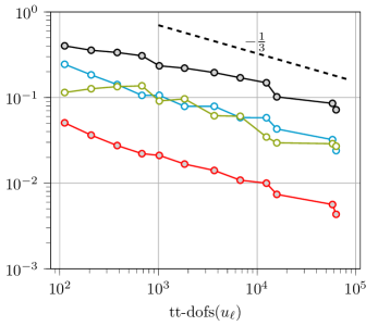
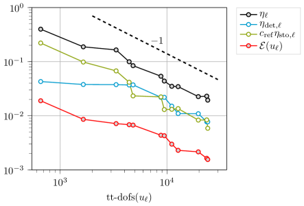
Figure 2: Reduction of estimator and error on the L-shaped domain for affine (left) and cubic (right) Lagrange finite elements with respect to the Tensor Train degrees of freedom of the Galerkin projection $u_{N}$.

Figure 2 depict the sampled root mean squared $H_{0}^{1}(D)$ error $\mathcal{E}(u_{\ell})$, the overall error estimator $\eta(u_{\ell})$ and the two estimator contributions $\eta_{\mathrm{det}}(u_{\ell})$ and $\eta_{\mathrm{sto}}(u_{\ell})$ for affine and cubic Lagrange finite elements, respectively. The plots depict error and estimator against the degrees of freedom (dofs) of the coefficient tensor of the Galerkin projection $u_{N}$ compressed by the Tensor Train format, i.e.

$$\operatorname{tt-dofs}(u_{N})=Jr_{1}-r_{1}^{2}+\sum_{m=1}^{M-1}(r_{m}d_{m}r_{m+1}-r_{m+1}^{2})+r_{M}d_{M},$$

where $r=(r_{1},\dots,r_{M})\in\mathbb{N}^{M}$ are the Tensor Train ranks, see e.g. [37] for details.

The estimator mirrors the behaviour of the error with a consistent overestimation by a factor $c_{\mathrm{rel}}\approx 10$, which is in line with Theorem 3.2. Additionally, the deterministic estimator contribution $\eta_{\mathrm{det}}$ captures the singularity of the L-shaped domain and prioritizes to refine the mesh at the reentrant corner as known from deterministic adaptive FE methods, which is in line with previous results [EGSZ14, 10, 3, 5, EMPS20]. We also observe that Algorithm 1 focusses on refinement of the finite element mesh for $p=1$ and tends to enlarge the stochastic space in the case $p=3$. Again, this is in line with the expectations, as the higher regularity of cubic finite elements allows for coarser spatial resolution.

Finally we note that the experiments are in line with the results of Theorem 5.2 as we observe a reduction of both error and estimator in each iteration. Interestingly, we even see that the algorithm reduces both error and estimator with an overall constant rate, which is consistent with the results of e.g. [7, 8]. This is a stronger behaviour than predicted by Theorem 5.2. An explanation of this could be that the diffusion coefficient is “effectively” bounded and positive by any experimental setup since only finitely many point evaluations can be used to generate the numerical representation of (2.2). This implies that $a$ is effectively only considered on a bounded domain, which yields boundedness from above and below as assumed in Corollary 5.4.

EGSZ14EigelGittelson2014asgfem EMPS20EigelMarschall2020lognormal

References

- [1] Martin Eigel, Claude Jeffrey Gittelson, Christoph Schwab and Elmar Zander “Adaptive stochastic Galerkin FEM” In Computer Methods in Applied Mechanics and Engineering 270 Elsevier BV, 2014, pp. 247–269 DOI: 10.1016/j.cma.2013.11.015
- [2] Alex Bespalov and David Silvester “Efficient Adaptive Stochastic Galerkin Methods for Parametric Operator Equations” In SIAM Journal on Scientific Computing 38.4 Society for Industrial & Applied Mathematics (SIAM), 2016, pp. A2118–A2140 DOI: 10.1137/15m1027048
- [3] Alex Bespalov and Leonardo Rocchi “Efficient Adaptive Algorithms for Elliptic PDEs with Random Data” In SIAM/ASA Journal on Uncertainty Quantification 6.1 Society for Industrial & Applied Mathematics (SIAM), 2018, pp. 243–272 DOI: 10.1137/17m1139928
- [4] Adam J. Crowder, Catherine E. Powell and Alex Bespalov “Efficient Adaptive Multilevel Stochastic Galerkin Approximation Using Implicit A Posteriori Error Estimation” In SIAM Journal on Scientific Computing 41.3 Society for Industrial & Applied Mathematics (SIAM), 2019, pp. A1681–A1705 DOI: 10.1137/18m1194420
- [5] Alex Bespalov, Dirk Praetorius and Michele Ruggeri “Two-Level a Posteriori Error Estimation for Adaptive Multilevel Stochastic Galerkin Finite Element Method” In SIAM/ASA Journal on Uncertainty Quantification 9.3 Society for Industrial & Applied Mathematics (SIAM), 2021, pp. 1184–1216 DOI: 10.1137/20m1342586
- [6] Markus Bachmayr and Igor Voulis “An adaptive stochastic Galerkin method based on multilevel expansions of random fields: Convergence and optimality” In ESAIM: Mathematical Modelling and Numerical Analysis 56.6 EDP Sciences, 2022, pp. 1955–1992 DOI: 10.1051/m2an/2022062
- [7] Martin Eigel, Manuel Marschall, Max Pfeffer and Reinhold Schneider “Adaptive stochastic Galerkin FEM for lognormal coefficients in hierarchical tensor representations” In Numerische Mathematik 145.3 Springer ScienceBusiness Media LLC, 2020, pp. 655–692 DOI: 10.1007/s00211-020-01123-1
- [8] Martin Eigel, Nando Farchmin, Sebastian Heidenreich and Philipp Trunschke “Adaptive non-intrusive reconstruction of solutions to high-dimensional parametric PDEs” arXiv, 2021 DOI: 10.48550/ARXIV.2112.01285
- [9] Martin Eigel, Claude Jeffrey Gittelson, Christoph Schwab and Elmar Zander “A convergent adaptive stochastic Galerkin finite element method with quasi-optimal spatial meshes” In ESAIM: Mathematical Modelling and Numerical Analysis 49.5 EDP Sciences, 2015, pp. 1367–1398 DOI: 10.1051/m2an/2015017
- [10] Alex Bespalov, Dirk Praetorius, Leonardo Rocchi and Michele Ruggeri “Convergence of Adaptive Stochastic Galerkin FEM” In SIAM Journal on Numerical Analysis 57.5 Society for Industrial & Applied Mathematics (SIAM), 2019, pp. 2359–2382 DOI: 10.1137/18m1229560
- [11] Alex Bespalov, Dirk Praetorius and Michele Ruggeri “Convergence and rate optimality of adaptive multilevel stochastic Galerkin FEM” In IMA Journal of Numerical Analysis 42.3 Oxford University Press (OUP), 2021, pp. 2190–2213 DOI: 10.1093/imanum/drab036
- [12] Martin Eigel, Oliver G. Ernst, Björn Sprungk and Lorenzo Tamellini “On the Convergence of Adaptive Stochastic Collocation for Elliptic Partial Differential Equations with Affine Diffusion” In SIAM Journal on Numerical Analysis 60.2 Society for Industrial & Applied Mathematics (SIAM), 2022, pp. 659–687 DOI: 10.1137/20m1364722
- [13] Peter Binev, Wolfgang Dahmen and Ron DeVore “Adaptive Finite Element Methods with convergence rates” In Numerische Mathematik 97.2 Springer ScienceBusiness Media LLC, 2004, pp. 219–268 DOI: 10.1007/s00211-003-0492-7
- [14] J. Cascon, Christian Kreuzer, Ricardo H. Nochetto and Kunibert G. Siebert “Quasi-Optimal Convergence Rate for an Adaptive Finite Element Method” In SIAM Journal on Numerical Analysis 46.5 Society for Industrial & Applied Mathematics (SIAM), 2008, pp. 2524–2550 DOI: 10.1137/07069047x
- [15] Willy Dörfler “A Convergent Adaptive Algorithm for Poisson’s Equation” In SIAM Journal on Numerical Analysis 33.3 Society for Industrial & Applied Mathematics (SIAM), 1996, pp. 1106–1124 DOI: 10.1137/0733054
- [16] Pedro Morin, Ricardo H. Nochetto and Kunibert G. Siebert “Data Oscillation and Convergence of Adaptive FEM” In SIAM Journal on Numerical Analysis 38.2 Society for Industrial & Applied Mathematics (SIAM), 2000, pp. 466–488 DOI: 10.1137/s0036142999360044
- [17] Rob Stevenson “The completion of locally refined simplicial partitions created by bisection” In Mathematics of Computation 77.261 American Mathematical Society (AMS), 2008, pp. 227–241 DOI: 10.1090/s0025-5718-07-01959-x
- [18] Yingbo Hua and Wanquan Liu “Generalized Karhunen-Loeve transform” In IEEE Signal Processing Letters 5.6 Institute of ElectricalElectronics Engineers (IEEE), 1998, pp. 141–142 DOI: 10.1109/97.681430
- [19] Markus Bachmayr, Albert Cohen, Ronald DeVore and Giovanni Migliorati “Sparse polynomial approximation of parametric elliptic PDEs. Part II: lognormal coefficients” In ESAIM: Mathematical Modelling and Numerical Analysis 51.1 EDP Sciences, 2017, pp. 341–363
- [20] Viet Ha Hoang and Christoph Schwab “N-term Wiener chaos approximation rates for elliptic PDEs with lognormal gaussian random inputs” In Mathematical Models and Methods in Applied Sciences 24.04 World Scientific Pub Co Pte Lt, 2014, pp. 797–826 DOI: 10.1142/s0218202513500681
- [21] C.. Gittelson “Stochastic Galerkin Discretization of the Log-Normal isotropic Diffusion Problem” In Mathematical Models and Methods in Applied Sciences 20.02 World Scientific Pub Co Pte Lt, 2010, pp. 237–263 DOI: 10.1142/s0218202510004210
- [22] Antje Mugler and Hans-Jörg Starkloff “On the convergence of the stochastic Galerkin method for random elliptic partial differential equations” In ESAIM: Mathematical Modelling and Numerical Analysis-Modélisation Mathématique et Analyse Numérique 47.5, 2013, pp. 1237–1263
- [23] J. Galvis and M. Sarkis “Approximating infinity-dimensional stochastic Darcy’s equations without uniform ellipticity” In SIAM J. Numer. Anal. 47.5, 2009, pp. 3624–3651 DOI: 10.1137/080717924
- [24] Christoph Schwab and Claude Jeffrey Gittelson “Sparse tensor discretizations of high-dimensional parametric and stochastic PDEs” In Acta Numerica 20 Cambridge University Press, 2011, pp. 291–467 DOI: 10.1017/S0962492911000055
- [25] Albert Cohen, Ronald DeVore and Christoph Schwab “Convergence Rates of Best N-term Galerkin Approximations for a Class of Elliptic sPDEs” In Foundations of Computational Mathematics 10.6 Springer ScienceBusiness Media LLC, 2010, pp. 615–646 DOI: 10.1007/s10208-010-9072-2
- [26] Albert Cohen, Ronald DeVore and Christoph Schwab “Analytic regularity and polynomial approximation of parametric and stochastic elliptic PDEs” World Scientific Pub Co Pte Lt, 2011, pp. 11–47 DOI: 10.1142/s0219530511001728
- [27] Mike Espig, Wolfgang Hackbusch, Alexander Litvinenko, Hermann G Matthies and Philipp Wähnert “Efficient low-rank approximation of the stochastic Galerkin matrix in tensor formats” In Computers & Mathematics with Applications 67.4 Elsevier, 2014, pp. 818–829
- [28] Sergey Dolgov and Robert Scheichl “A Hybrid Alternating Least Squares–TT-Cross Algorithm for Parametric PDEs” In SIAM/ASA Journal on Uncertainty Quantification 7.1 Society for Industrial & Applied Mathematics (SIAM), 2019, pp. 260–291 DOI: 10.1137/17m1138881
- [29] Martin Eigel, Nando Farchmin, Sebastian Heidenreich and P. Trunschke “Efficient approximation of high-dimensional exponentials by tensor networks” In International Journal for Uncertainty Quantification 13.1 Begell House, 2023, pp. 25–51 DOI: 10.1615/int.j.uncertaintyquantification.2022039164
- [30] D. Braess “Finite elements” Theory, fast solvers, and applications in elasticity theory, Translated from the German by Larry L. Schumaker Cambridge University Press, Cambridge, 2007, pp. xviii+365 DOI: 10.1017/CBO9780511618635
- [31] Martin Eigel, Reinhold Schneider, Philipp Trunschke and Sebastian Wolf “Variational Monte Carlo—bridging concepts of machine learning and high-dimensional partial differential equations” In Advances in Computational Mathematics 45.5-6 Springer ScienceBusiness Media LLC, 2019, pp. 2503–2532 DOI: 10.1007/s10444-019-09723-8
- [32] Martin Eigel, Reinhold Schneider and Philipp Trunschke “Convergence bounds for empirical nonlinear least-squares” In ESAIM: Mathematical Modelling and Numerical Analysis 56.1 EDP Sciences, 2022, pp. 79–104 DOI: 10.1051/m2an/2021070
- [33] Philipp Trunschke “Convergence bounds for nonlinear least squares and applications to tensor recovery”, 2021 arXiv:2108.05237 [math.NA]
- [34] Martin Alnæs, Jan Blechta, Johan Hake, August Johansson, Benjamin Kehlet, Anders Logg, Chris Richardson, Johannes Ring, Marie E Rognes and Garth N Wells “The FEniCS Project Version 1.5” In Archive of Numerical Software Vol 3 University Library Heidelberg, 2015, pp. 9–23 DOI: 10.11588/ANS.2015.100.20553
- [35] I.. Oseledets “Tensor-Train Decomposition” In SIAM Journal on Scientific Computing 33.5 Society for Industrial & Applied Mathematics (SIAM), 2011, pp. 2295–2317 DOI: 10.1137/090752286
- [36] Benjamin Huber and Sebastian Wolf “Xerus - A General Purpose Tensor Library”, https://libxerus.org/, 2014–2021
- [37] Sebastian Holtz, Thorsten Rohwedder and Reinhold Schneider “On manifolds of tensors of fixed TT-rank” In Numerische Mathematik 120.4 Springer ScienceBusiness Media LLC, 2011, pp. 701–731 DOI: 10.1007/s00211-011-0419-7