On symmetry breaking for the Navier-Stokes equations

Abstract.

Inspired by an open question by Chemin and Zhang about the regularity of the 3D Navier-Stokes equations with one initially small component, we investigate symmetry breaking and symmetry preservation. Our results fall in three classes. First we prove strong symmetry breaking. Specifically, we demonstrate third component norm inflation (3rdNI) and Isotropic Norm Inflation (INI) starting from zero third component. Second we prove symmetry breaking for initially zero third component, even in the presence of a favorable initial pressure gradient. Third we study certain symmetry preserving solutions with a shear flow structure. Specifically, we give applications to the inviscid limit and exhibit explicit solutions that inviscidly damp to the Kolmogorov flow.

1. Introduction

Symmetries preserved by evolution play an important role in the mathematical theory of the Navier-Stokes equations and Euler equations:

$$\partial_{t}{u^{\nu}}+u^{\nu}\cdot\nabla u^{\nu}+\nabla P =\nu\Delta u^{\nu}\quad \hbox{in }{\mathbb{R}}_{+}\times{\mathbb{T}}^{3},\quad\hbox{\rm div}\,u^{\nu} =0,\quad\nu\geq 0.$$ (1.1)

On the one hand, certain preserved symmetries lead to the preservation of certain structures that grant smoothness of solutions [33], [41]. On the other hand, preserved symmetries reduce the number of degrees of freedom of the Navier-Stokes and Euler equations, which can make it possible to prove or numerically investigate the existence of singularities [22], [14], [26, 27].

In this vein, in recent years there has been a substantial amount of activity aimed at showing that additional assumptions of one component of the velocity field (solving the Navier-Stokes equations) imply that the solution is regular. On the other side of coin, this corresponds to showing that solutions of the Navier-Stokes equations that become singular must do so in an isotropic manner. Research in this direction was initiated in the seminal paper of Neustupa and Penel [37]. Since then there have been many contributions to one-component regularity for the Navier-Stokes equations, with recent contributions showing regularity provided that one-component of the velocity field has a finite norm either almost preserved [10, 11] or preserved with respect to the Navier-Stokes scaling symmetry [12, 13, 43].

The purpose of this paper is to understand the dynamics of the Navier-Stokes equations when one-component of the initial data is zero. Throughout we will set the third component of the initial data to be zero, without loss of generality. Our main motivation is an open question raised by Chemin, Zhang and Zhang [13] when discussing endpoint one-component regularity criteria. Specially, in [13, page 873], Chemin, Zhang and Zhang formulate the following open question:

(Q) [If] for some unit vector $e$ of ${\mathbb{R}}^{3}$, [the component of the initial data] $\|u_{\rm in}\cdot e\|_{H^{\frac{1}{2}}}$ is small with respect to some universal constant, is it implied that there is no blow up for the Fujita-Kato solution of (NS)?

1.1. Main results of the paper

In relation to the aforementioned open problem (Q), our first two results show that initial data with zero third component can exhibit third component norm inflation (3rdNI, Theorem A) and Isotropic Norm Inflation (INI, Theorem A’) with respect to critical norms specified in [7].

Theorem A (strong symmetry breaking).

For any $0<\delta<1$, there exists mean-free $C^{\infty}({\mathbb{T}}^{3})$ solenoidal initial data $u_{\rm in}$ and $\bar{u}_{\rm in}$ with vanishing third component,

$$\|u_{\rm in}-\bar{u}_{\rm in}\|_{\dot{B}^{-1}_{\infty,\infty}}=\|u_{\rm in}^{\rm h}-\bar{u}_{\rm in}^{\rm h}\|_{\dot{B}^{-1}_{\infty,\infty}}<\delta,$$

and such that the following holds true.
There exists a unique solution $u$ $({\rm resp.}~{}\bar{u})$ of the Cauchy problem (1.1) subject to initial data $u_{\rm in}$ (resp. $\bar{u}_{\rm in}$) belonging to $C^{\infty}((0,T]\times{\mathbb{T}}^{3})$ for some time $0<T<\delta$ with $\bar{u}^{3}\equiv 0$ on $[0,T]\times{\mathbb{R}}^{3}$ and

$$\|u^{3}{(T,\cdot)}-\bar{u}^{3}{(T,\cdot)}\|_{\dot{B}^{-1}_{\infty,\infty}}=\|u^{3}{(T,\cdot)}\|_{\dot{B}^{-1}_{\infty,\infty}}>\frac{1}{\delta}.$$

Moreover,

$$\min\big{(}\|u^{1}{(T,\cdot)}\|_{L^{3}},\|u^{2}{(T,\cdot)}\|_{L^{3}},\|u^{3}{(T,\cdot)}\|_{L^{3}}\big{)}>\frac{1}{\delta}.$$ (1.2)

Theorem A does not provide negative evidence towards (Q), but demonstrates that regularity in that case can only be granted by a yet to be discovered mechanism unrelated to the preservation of smallness of the third component of the corresponding solution. However, the solution in Theorem A remains small in $\dot{B}^{-1}_{\infty,\infty}$ at $T$ in certain directions (see the discussion in subsection 1.3). Thus, the construction in Theorem A does not rule out the possibility that solutions, with initial third component equal to zero, remain small along some time-varying direction. Such a possibility is in fact ruled out by our second result below.

Theorem A’ (strong isotropic symmetry breaking).

For any $0<\delta<1$, there exists mean-free $C^{\infty}({\mathbb{T}}^{3})$ solenoidal initial data $u_{\rm in}$ and $\bar{u}_{\rm in}$ with vanishing third component,

$$\|u_{\rm in}-\bar{u}_{\rm in}\|_{\dot{B}^{-1}_{\infty,\infty}}=\|u_{\rm in}^{\rm h}-\bar{u}_{\rm in}^{\rm h}\|_{\dot{B}^{-1}_{\infty,\infty}}<\delta,$$

and such that the following holds true.
There exists a unique solution $u$ of the Cauchy problem (1.1) subject to initial data $u_{\rm in}$ belonging to $C^{\infty}((0,T]\times{\mathbb{T}}^{3})$ for some time $0<T<\delta$ and such that

$${\inf_{\mathbf{e}\in\mathbb{R}^{3}:|\mathbf{e}|=1}\|u(T,\cdot)\cdot\mathbf{e}\|_{\dot{B}^{-1}_{\infty,\infty}}>\frac{1}{\delta}.}$$ (1.3)

We dub the norm inflation in all directions in (1.3) ‘Isotropic Norm Inflation’ (INI).

Now define the initial pressure $P_{\rm in}$ associated to the initial data $u_{\rm in}$, which satisfies

$$-\Delta P_{\rm in}:=\nabla u_{\rm in}:(\nabla u_{\rm in})^{\rm T}.$$ (1.4)

Note that the initial data used to prove Theorems A and A’, which will heuristically be described in subsections 1.2-1.3, both necessarily generate an initial pressure $P_{\rm in}$ that satisfies $\partial_{3}P_{\rm in}\neq 0.$ From the equation for the third component of the associated solution (1.1), it is qualitatively clear that such an initial pressure will always produce a solution that breaks the symmetry of the third component zero. In this regard, we call pressure of this type unfavorable. Notice that there are other examples of plane-wave initial data that demonstrate symmetry breaking. We refer for instance to Figure 1 that shows breaking for the Taylor-Green vortex

$$u_{in}(x_{1},x_{2},x_{3})=(\sin x_{1}\cos x_{2}\cos x_{3},-\cos x_{1}\sin x_{2}\cos x_{3},0).$$

Notice that

$$\Delta P_{in}=2(\cos x_{3})^{2}\big{(}(\cos x_{1}\cos x_{2})^{2}-(\sin x_{1}\sin x_{2})^{2}\big{)}$$

so that the pressure for the Taylor-Green vortex is also unfavorable.

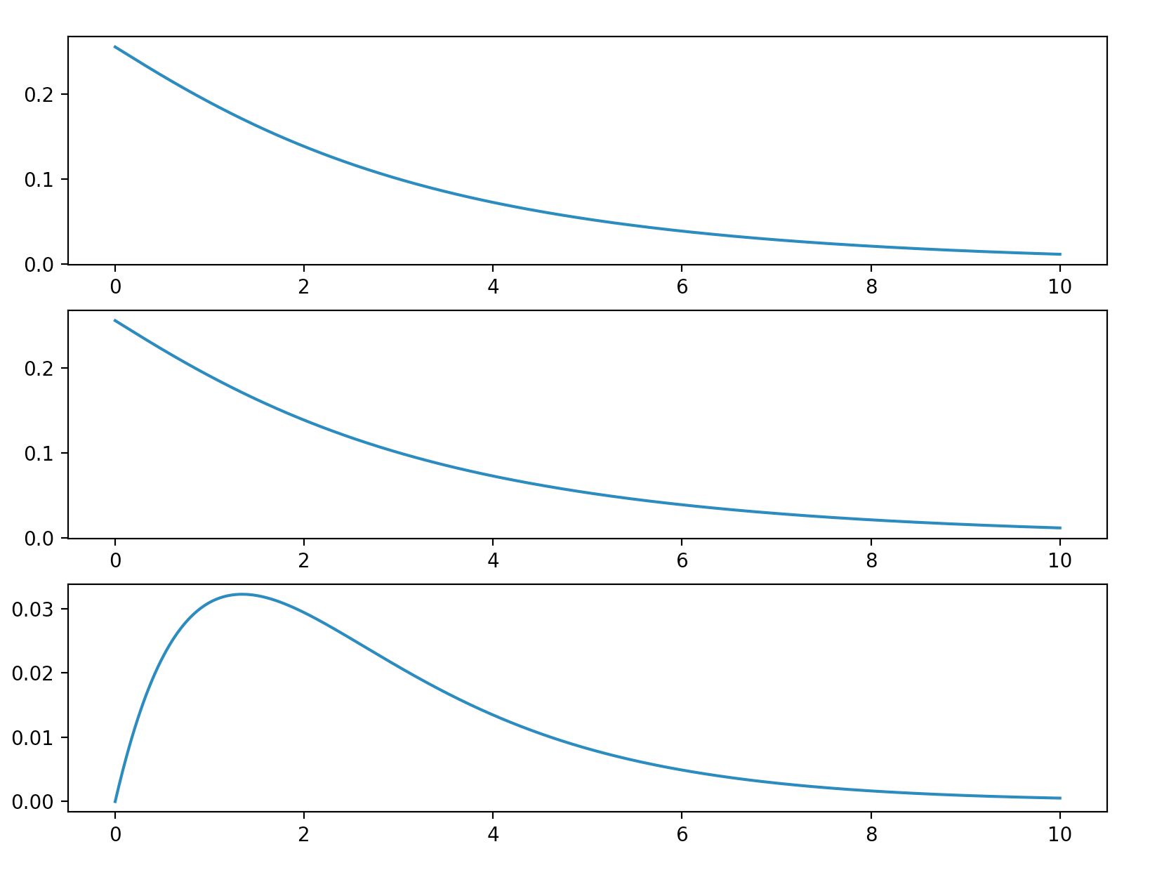
Figure 1. Taylor-Green vortex solution of Navier-Stokes with viscosity $\nu=10^{-1}$. From top to bottom: $\|u^{1}(\cdot,t)\|_{L^{1}({\mathbb{T}}^{3})}$, $\|u^{2}(\cdot,t)\|_{L^{1}({\mathbb{T}}^{3})}$ and $\|u^{3}(\cdot,t)\|_{L^{1}({\mathbb{T}}^{3})}$. This simulation shows breaking with initial pressure unfavorable (see Footnote 4 for a definition) to symmetry preservation. Choice of parameters: total time $T=10$ and time step $dt=10^{-2}$; spectral code by Mikael Mortensen taken from https://github.com/spectralDNS/spectralDNS with $(2^{5})^{3}$ mesh points.

As a consequence of the above, for initial data $u_{\rm in}$ with zero third component, we say that an initial pressure $P_{\rm in}$ is favorable if

$$\hbox{\rm div}_{\rm h}u^{\rm h}_{\rm in}=0\quad{\rm with}\quad\partial_{3}P_{\rm in}=0,\quad{\rm where}~{}-\Delta P_{\rm in}:=\nabla_{\rm h}u^{\rm h}_{\rm in}:(\nabla_{\rm h}u^{\rm h}_{\rm in})^{\rm T}.$$ (1.5)

For a favorable initial pressure, the equation for the third component of (1.1) does not immediately imply that the third component of the solution breaks symmetry and becomes non-zero. In the Theorem below we are able to demonstrate an initial data below, which has zero third component and favorable initial pressure, yet the corresponding solution breaks the symmetry and has non-zero third component on some time interval.

Theorem B (symmetry breaking despite favorable pressure gradient).

We consider the initial data

$$u_{\rm in}{=}\left(\cos x_{2}\,\frac{N}{N+\sin x_{3}},\,\cos x_{1}\,\frac{N+\sin x_{3}}{N},\,0\right)$$ (1.6)

which has favorable initial pressure gradient in the sense that $\partial_{3}P_{in}=0$, see (1.5).
Then there exists a positive constant $N_{0}$ such that for any $N>N_{0},$ the initial data given by (1.6) generates a unique solution $u$ to the Navier-Stokes equations (1.1) on $[0,1]\times{\mathbb{T}}^{3}$ that satisfies

$$\|u^{3}(t,\cdot)\|_{L^{\infty}({\mathbb{T}}^{3})}\sim\frac{t^{2}}{N^{2}},$$ (1.7)

for any $0\leq t\leq\frac{1}{N^{2}}\ll 1$.

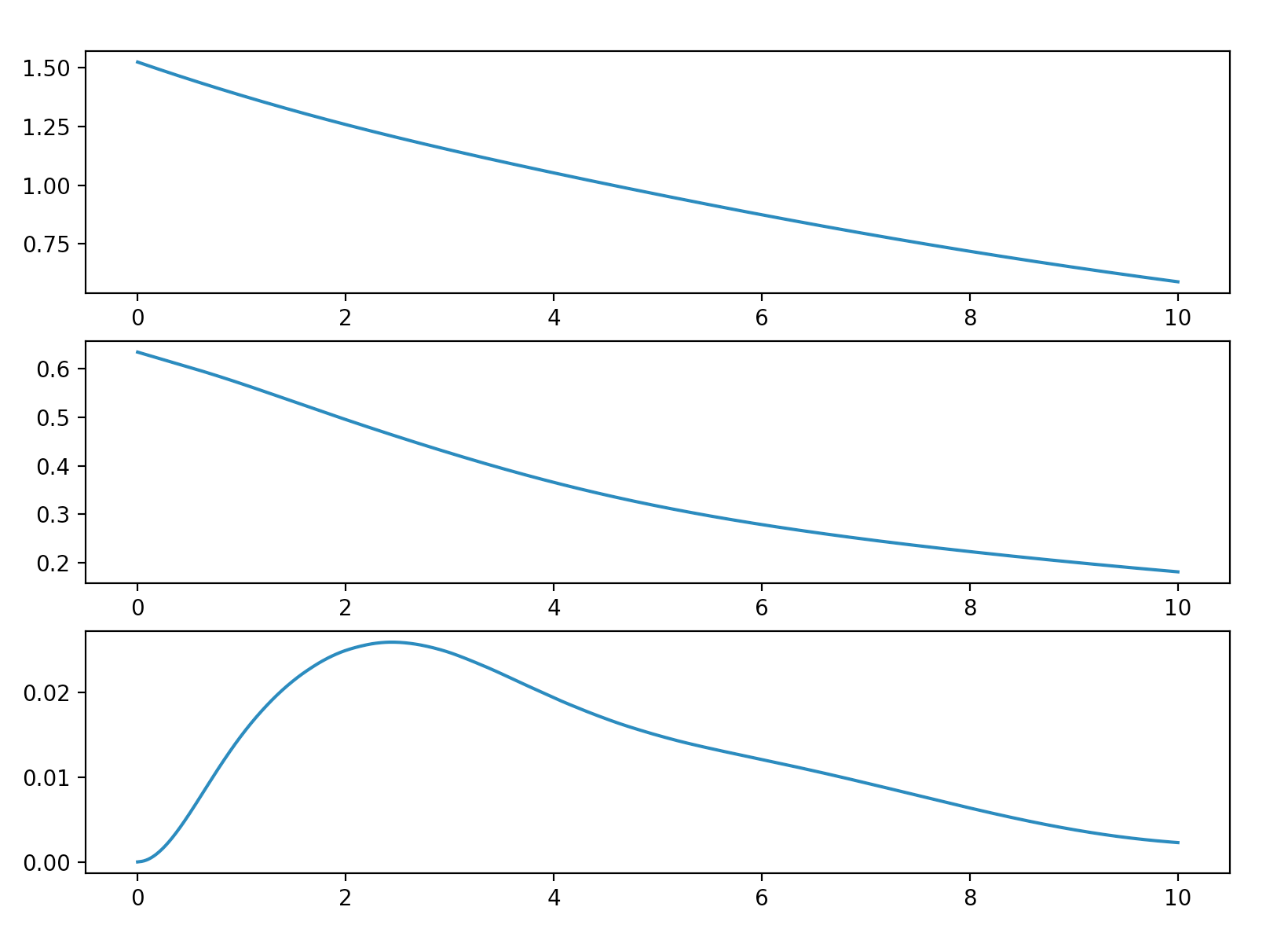
Figure 2. Simulation of the Navier-Stokes equations with viscosity $\nu=10^{-1}$ and initial data from Theorem B taking $N=1.1$. From top to bottom: $\|u^{1}(\cdot,t)\|_{L^{1}({\mathbb{T}}^{3})}$, $\|u^{2}(\cdot,t)\|_{L^{1}({\mathbb{T}}^{3})}$ and $\|u^{3}(\cdot,t)\|_{L^{1}({\mathbb{T}}^{3})}$. This simulation shows breaking despite initial pressure favorable (see Footnote 5 for a definition) to symmetry preservation. Choice of parameters: total time $T=10$ and time step $dt=10^{-2}$; spectral code by Mikael Mortensen taken from https://github.com/spectralDNS/spectralDNS with $(2^{5})^{3}$ mesh points.

Remark 1 (comparison to other symmetry breaking results).

The non-uniqueness numerical results of Guillod and Šverák [24] concern Leray-Hopf solutions of the Navier-Stokes equations that break a symmetry class. In the context of the Euler equations and convex integration, symmetry breaking and restoration mechanisms were explicitly investigated in [2]. The non-uniqueness results for dissipative solutions of Euler by Scheffer [38], Shnirelman [40], De Lellis and Székelyhidi [21], Isett [29] and for weak solutions of Navier-Stokes by Buckmaster and Vicol [8] can also be seen as symmetry breaking results. Our results are in a different vein though. We show breaking of symmetry on some time interval where the solution is unique and smooth.

Remark 2 (isotropic motion with initial third component zero).

For the construction in Theorem A’, one can also show that for all $\mathbf{e}\in\mathbb{R}^{3}$ with $|\mathbf{e}|=1$:

$$\|u(T,\cdot)\cdot\mathbf{e}\|_{\dot{B}^{-1}_{\infty,\infty}}\sim\frac{1}{\delta}.$$

Thus at time $T$, the velocity field is comparable in all unit directions with respect to the $\dot{B}^{-1}_{\infty,\infty}$ norm, despite evolving from initial data with zero third component.

Further results

Our interest here is on flows that preserve the symmetry $u_{3}=0$ and on applications of such flows.

There are indeed flows solving Navier-Stokes and Euler that have a shear-flow structure and keep the third component identically zero, as for instance the plane parallel channel flows $(u^{1}(x_{3},t),u^{2}(x_{1},x_{3},t),0)$ introduced by Wang [44]. Rotating these flows gives rise to a whole family of symmetry preserving pressureless shear flows that we dub ‘2.75D shear flows’, which are defined as follows. Let $\lambda\in\mathbb{Z}$ be a constant. Consider the initial data

$$u_{\rm in}=\big{(}f(\lambda x_{1}+x_{2},x_{3}),\,-\lambda f(\lambda x_{1}+x_{2},x_{3})-g(x_{3}),0\big{)},\quad x\in{\mathbb{T}}^{3}.$$ (1.8)

In fact, in the case that $u_{\rm in}$ merely belongs to $L^{2}({\mathbb{T}}^{3})$ (that corresponds to $f$ or $g$ being rough), one can obtain a Leray-Hopf weak solution to the problem (1.1) with $\nu>0$, and initial data $u_{\rm in}$, given by

$$u^{\nu}=\big{(}F_{\nu}(t,\lambda x_{1}+x_{2},x_{3}),-\lambda F_{\nu}(t,\lambda x_{1}+x_{2},x_{3})-e^{\nu t\partial_{3}^{2}}g(x_{3}),0\big{)}$$ (1.9)

where $F_{\nu}:{\mathbb{R}}_{+}\times{\mathbb{T}}^{2}\to{\mathbb{R}}$ is the unique global-in-time solution to

$$\left\{\begin{aligned} &\partial_{t}F_{\nu}-e^{\nu t\partial_{2}^{2}}g(y_{2})\,\partial_{1}F_{\nu}=\nu\bigl{(}(\lambda^{2}+1)\partial_{1}^{2}+\partial_{2}^{2}\bigr{)}F_{\nu}\quad{\rm in}~{}~{}{\mathbb{T}}^{2}\times{\mathbb{R}}_{+}\\ &F_{\nu}(0,y_{1},y_{2})=f(y_{1},y_{2}).\end{aligned}\right.$$ (1.10)

For more insights about the derivation of these flows, we refer to Appendix A.

Remark 3 (2.75D shear flows for Euler).

One also has ‘2.75D shear flows’ that solve the Euler equations in a distributional sense:

$$u^{E}(t,x)=\big{(}f(\lambda x_{1}+x_{2}+tg(x_{3}),x_{3}),-\lambda f(\lambda x_{1}+x_{2}+tg(x_{3}),x_{3})-g(x_{3}),0\big{)},$$ (1.11)

where $f\in L^{2}({\mathbb{T}}^{3})$ and $g\in C^{\infty}({\mathbb{T}}^{2})$.

Inviscid damping

In Section 4.1 we show that the 2.75D shear flows for Euler, see Remark 3, inviscidly damp to the Kolmogorov flow $u^{K}=(0,\sin x_{3},0)$. The Kolmogorov flow is a stationary solution of the 3D Euler equations in $\mathbb{T}^{3}$. In [20] Coti-Zelati, Elgindi and Widmayer exhibit 2D stationary solutions to the Euler equations near $u^{K}$, thus demonstrating a lack of inviscid damping near $u^{K}$. On the other hand, 2.75D shear Euler flows (1.11) can be used to produce explicit solutions that inviscidly damp to $u^{K}$ for large times. This and [20] show that dynamics near the Kolmogorov flow in $\mathbb{T}^{3}$ are rich and no generic behavior can be expected.

Vanishing viscosity

In Section 4.2 we investigate the vanishing viscosity limit for 2.75D shear flow solutions of Navier-Stokes that are Onsager supercritical. Turbulence theory from [30, 31, 32] predicts that if $u^{\nu}$ is a weak Leray-Hopf solution in $\mathbb{T}^{3}\times(0,\infty)$, with viscosity $\nu$ and initial data $u_{\rm in}$, then generically one has anomalous dissipation:

$$\liminf_{\nu\rightarrow 0}\nu\int\limits\limits_{0}^{T}\int\limits\limits_{\mathbb{T}^{3}}|\nabla u^{\nu}|^{2}dxds>0.$$ (1.12)

It is known that if (1.12) and the vanishing viscosity limit holds in suitable topology, then the corresponding Euler flow $u^{E}$ must belong to Onsager supercritical spaces such as $C^{\frac{1}{3}-}$ or $\dot{H}^{\frac{5}{6}-}$. See [19] and [15], for example.

Using 2.75D shear flows for the Navier-Stokes and Euler equations, we show in Propositions 4.1 and 4.2 that the vanishing viscosity limit and the corresponding Euler flow belonging to Onsager supercritical spaces are not sufficient conditions for anomalous dissipation. Moreover in Proposition 4.1, we build upon the work of [4] to give an example of a rough solution to the 3D Euler equations that satisfies the local energy balance.

1.2. Heuristics for strong symmetry breaking

In this subsection, we give some heuristics for Theorem A.

The mechanism to get norm inflation in the critical $\dot{B}^{-1}_{\infty,\infty}$ space is well understood thanks to the work of Bourgain and Pavlović [7], and later Yoneda [45] and Cheskidov and Dai [16]. We mention here also the work of Wang [42], which demonstrates norm inflation phenomena in the spaces $\dot{B}^{-1}_{\infty,q}$ for $1\leq q\leq 2$, but the construction is different from the one considered here.

Our point here is to explain how to get norm inflation on the third component (3rdNI), starting from data with third component equal to zero as in the case of Theorem A. Such norm inflation on the third component cannot be obtained from the previously known constructions.

As a starting point, let us consider the general plane-wave initial data

$$\kappa(r)\sum_{j=1}^{r}A_{j}\big{(}\mathbf{v}\cos(\mathbf{k_{j}}\cdot x)+\mathbf{v^{\prime}}\cos(\mathbf{k_{j}^{\prime}}\cdot x)\big{)}.$$ (1.13)

Here $\mathbf{v},\,\mathbf{v^{\prime}}\in{\mathbb{R}}^{3}$ are fixed constant vectors, $\kappa(r)$ is some function such that $\kappa(r)\rightarrow 0$ when $r\rightarrow\infty$, $A_{j}\in[0,\infty)$ is a sequence of amplitudes growing geometrically, and $k_{j}\,k_{j}^{\prime}\in{\mathbb{R}}^{3}$ are two sequences of vectors whose magnitudes grow at a geometric rate. Hence the initial data given by (1.13) is a superposition of highly oscillating plane waves. This data covers the situations studied in [7, 45, 16]. In all these studies, $\kappa(r)$ and the sequence $A_{j}$ need to be finely tuned in order to produce a small $\dot{B}^{-1}_{\infty,\infty}$ norm at initial time but a large one after an arbitrarily short time.

We now describe the geometric constraints that we put on the vectors $\mathbf{v}$, $\mathbf{v^{\prime}}$, $\mathbf{k_{j}}$ and $\mathbf{k_{j}^{\prime}}$. There are two obvious conditions. First, in order to satisfy the divergence-free condition, we impose

$$\mathbf{v}\cdot\mathbf{k}_{j}=0=\mathbf{v}^{\prime}\cdot\mathbf{k}_{j}^{\prime}.$$ (3rdNI Condition 1)

Second, in order to have vertical velocity zero initially, we impose

$$\mathbf{v}\cdot\mathbf{e}_{3}=\mathbf{v^{\prime}}\cdot\mathbf{e}_{3}=0$$ (3rdNI Condition 2)

where $\mathbf{e}_{3}$ is the third vector of the canonical basis of ${\mathbb{R}}^{3}$. In order to produce norm inflation in $\dot{B}^{-1}_{\infty,\infty}$ from this superposition of highly oscillating plane waves, one needs to produce a non-oscillating function from the interaction of the term oscillating with wavenumber $\mathbf{k_{j}}$ and the term oscillating with wavenumber $\mathbf{k_{j}^{\prime}}$. Hence, following [7, 45, 16], we impose that there exists a fixed constant vector $\boldsymbol{\eta}\in{\mathbb{R}}^{3}$ such that

$$\mathbf{k_{j}}-\mathbf{k_{j}^{\prime}}=\boldsymbol{\eta}.$$ (3rdNI Condition 3)

The norm inflation mechanism can be seen as a backward energy cascade, producing large-scale, non-oscillating, structures from small-scale, highly oscillating, structures.

We now investigate the conditions needed to get norm inflation of the third component. A computation of the second Duhamel iterate leads to the following inflation term

$$\kappa(r)^{2}\sum_{j=1}^{r}\Big{(}\int\limits_{0}^{t}e^{-(|\mathbf{k_{j}}|^{2}+|\mathbf{k_{j}^{\prime}}|^{2})(t-s)}ds\Big{)}\mathbb{P}\big{(}\sin(\boldsymbol{\eta}\cdot x)((\mathbf{v}\cdot\mathbf{k_{i}^{\prime}})\mathbf{v^{\prime}}-(\mathbf{v^{\prime}}\cdot\mathbf{k_{j}})\mathbf{v}\big{)}.$$ (1.14)

Notice that the third component of

$$\sin(\boldsymbol{\eta}\cdot x)((\mathbf{v}\cdot\mathbf{k_{i}^{\prime}})\mathbf{v^{\prime}}-(\mathbf{v^{\prime}}\cdot\mathbf{k_{j}})\mathbf{v})$$ (1.15)

is zero. Hence, in order to get norm inflation on the third component, one needs the quantity in (1.15) to have a non-zero divergence, which will impose further constraints on $\mathbf{k_{i}},\ \mathbf{k_{i}^{\prime}},\ \mathbf{v},\ \mathbf{v^{\prime}}$ and $\boldsymbol{\eta}$. This is in stark contrast with previous studies [7, 45, 16], where the quantity in (1.15) is divergence-free and hence the norm inflation term remains in the span of $\mathbf{v}$ and $\mathbf{v^{\prime}}$.

Computing the Helmholtz-Leray projection in the norm inflation term (1.14) we get

$$\begin{split}&\mathbb{P}\big{(}\sin(\boldsymbol{\eta}\cdot x)((\mathbf{v}\cdot\mathbf{k_{j}^{\prime}})\mathbf{v^{\prime}}-(\mathbf{v^{\prime}}\cdot\mathbf{k_{j}})\mathbf{v}\big{)}\\ &=\sin(\boldsymbol{\eta}\cdot x)\Big{(}(\mathbf{v}\cdot\mathbf{k_{j}^{\prime}})\mathbf{v^{\prime}}-(\mathbf{v^{\prime}}\cdot\mathbf{k_{j}})\mathbf{v}-\frac{\boldsymbol{\eta}}{|\boldsymbol{\eta}|^{2}}\big{(}(\mathbf{v}\cdot\mathbf{k_{j}^{\prime}})(\mathbf{v^{\prime}}\cdot\boldsymbol{\eta})-(\mathbf{v^{\prime}}\cdot\mathbf{k_{j}})(\mathbf{v}\cdot\boldsymbol{\eta})\big{)}\Big{)}.\end{split}$$ (1.16)

Therefore, we need

$$\boldsymbol{\eta}\cdot\mathbf{e}_{3}\neq 0$$ (3rdNI Condition 4)

and

$$(\mathbf{v}\cdot\mathbf{k_{j}^{\prime}})(\mathbf{v^{\prime}}\cdot\boldsymbol{\eta})-(\mathbf{v^{\prime}}\cdot\mathbf{k_{j}})(\mathbf{v}\cdot\boldsymbol{\eta})\neq 0$$

in order to have norm inflation on the third component of the velocity. Using (3rdNI Condition 1) we can rewrite the last condition as

$$(\mathbf{v}\cdot\mathbf{k_{j}^{\prime}})(\mathbf{v^{\prime}}\cdot\mathbf{k_{j}})\neq 0$$

i.e.

$$\mathbf{v}\cdot\mathbf{k_{j}^{\prime}}\neq 0\quad\mbox{and}\quad\mathbf{v}^{\prime}\cdot\mathbf{k_{j}}\neq 0.$$ (3rdNI Condition 5)

Notice that conditions (3rdNI Condition 1)-(3rdNI Condition 5) are necessary but also sufficient to have norm inflation on the third component. There are many possible choices within the constraints (3rdNI Condition 1)-(3rdNI Condition 5). In particular, taking

$$\mathbf{v}=(1,-\lambda,0)\quad\mbox{and}\quad\mathbf{k_{j}}=(\lambda,1,2^{j-1}K)$$

for $\lambda,\,K\in{\mathbb{Z}}$, one has a whole family of initial data with $u_{\rm in}^{3}=0$ that produces norm inflation on the third component in $\dot{B}^{-1}_{\infty,\infty}$ and such that $u_{\rm in}$ is close in $\dot{B}^{-1}_{\infty,\infty}$ to a 2.75D shear flow initial data defined in (1.8).

1.3. Heuristics for strong isotropic symmetry breaking

From the previous subsection, notice that for initial data of the form

$$\kappa(r)\sum_{j=1}^{r}A_{j}\big{(}\mathbf{v}\cos(\mathbf{k_{j}}\cdot x)+\mathbf{v^{\prime}}\cos(\mathbf{k_{j}^{\prime}}\cdot x)\big{)}$$

that satisfies (3rdNI Condition 1)-(3rdNI Condition 5), the associated inflation term (1.16) vanishes in the direction $\boldsymbol{\eta}$. Here

$$\mathbf{k_{j}}-\mathbf{k_{j}^{\prime}}=\boldsymbol{\eta}\quad\textrm{for}\,\textrm{all}\,j.$$ (1.17)

This represents a block in using such initial data for obtaining the isotropic norm inflation (1.3) in Theorem A’.

To overcome this, we instead take initial data of the form

$$\kappa(r)\sum_{j=1}^{r^{3}}A_{j}\big{(}\mathbf{v_{j}}\cos(\mathbf{k_{j}}\cdot x)+\mathbf{v_{j}^{\prime}}\cos(\mathbf{k_{j}^{\prime}}\cdot x)\big{)}$$

$$\textrm{with}\quad\mathbf{k_{j}}-\mathbf{k_{j}^{\prime}}=\boldsymbol{\eta_{j}}.$$ (1.18)

Here, $\mathbf{v_{j}}$ and $\mathbf{v_{j}^{\prime}}$ vary with $j$ and crucially the low frequency vector $\boldsymbol{\eta_{j}}$ points in different directions depending on the index $j$. Specifically, we glue higher frequency terms to the initial data in Theorem A, such that the added terms $\mathbf{v_{j}}$,$\mathbf{v_{j}^{\prime}}$ and $\boldsymbol{\eta_{j}}$ point in different directions depending on $j$.

The initial data we design in Theorem A’ can be decomposed into three pieces $u_{\rm in}=u_{\rm in}^{(1)}+u_{\rm in}^{(2)}+u_{\rm in}^{(3)}$ such that

• each $u_{\rm in}^{(1)}$-$u_{\rm in}^{(3)}$ separately generate an associated Navier-Stokes solution with a norm inflation term, with each of these norm inflation terms being of comparable size in $\dot{B}^{-1}_{\infty,\infty}$,

• the norm inflation term associated to $u_{\rm in}$ is the sum of the norm inflation terms associated to $u_{\rm in}^{(1)}$-$u_{\rm in}^{(3)}$.

Careful choices of $\mathbf{v_{j}}$, $\mathbf{v_{j}^{\prime}}$, $\mathbf{k_{j}}$ and $\mathbf{k_{j}^{\prime}}$ then give that the norm inflation terms associated to $u_{\rm in}^{(1)}$-$u_{\rm in}^{(3)}$ point in linearly independent directions. This, together with our choices of $\mathbf{v_{j}}$, $\mathbf{v_{j}^{\prime}}$, $\mathbf{k_{j}}$ and $\mathbf{k_{j}^{\prime}}$ and the fact that $\dot{B}^{-1}_{\infty,\infty}$ is an $L^{\infty}$-based space, enable us to show that for any fixed unit vector $\mathbf{e}$

• (i) the dot product of $\mathbf{e}$ with at least one of the norm inflation terms associated to $u_{\rm in}^{(1)}$-$u_{\rm in}^{(3)}$ has a $\dot{B}^{-1}_{\infty,\infty}$ norm with a large lower bound,

• (ii) the lower bound in (i) also serves as a lower bound for the $\dot{B}^{-1}_{\infty,\infty}$ norm of the dot product of $\mathbf{e}$ with the norm inflation term associated to $u_{\rm in}$.

These features then imply that $u_{\rm in}$ generates a norm inflation term that has large $\dot{B}^{-1}_{\infty,\infty}$ norm in all unit directions. This in turn leads to the results described in Theorem A’.

1.4. Heuristics for symmetry breaking despite favorable pressure gradient

In this subsection, we give some heuristics for Theorem B.

Let us first explain how we design the initial data. Our objective is to find an initial data that will generate symmetry breaking despite favorable initial pressure (see Footnote 5). The two fractions in $u_{\rm in}$ are there to fulfill the condition $\partial_{3}P_{\rm in}\equiv 0$, where $P_{\rm in}$ is defined by (1.4). We also remark that the order in $t$ in (1.7) is expected because $\partial_{3}P_{\rm in}=0$ at $t=0$ formally implies that $\partial_{t}u_{3}=0$ at $t=0$. The breaking is not driven by the vertical derivative of the pressure at the initial time, as is the case in Theorem A and for the Taylor-Green vortex, see Figure 1.

In our proof, the condition $N>N_{0}$ appears for technical reasons in order to identify the leading order term. Indeed, for $N$ large, the term involving $S_{1}$ is the dominant term in the right hand side of (3.22). Notice also that the larger the $N$, the closer our data is from the two-dimensional data $(\cos x_{2},\cos x_{1},0)$ that generates a unique global two-dimensional solution to 3D Navier-Stokes. This has two implications. First, one sees, that $u_{\rm in}$ generates a unique solution to the 3D Navier-Stokes equations on ${\mathbb{T}}^{3}\times[0,1]$ for $N$ large. Second, the larger the $N$, the weaker the symmetry breaking effect should be. This observation is consistent with the bound $O(t^{2}/N^{2})$ in (1.7).

Remark 4 (on the condition $N\gg 1$ in Theorem B).

Figure 2 shows a simulation of the Navier-Stokes equations with initial data from Theorem B taking $N=1.1$. The graph shows that symmetry breaking happens in spite of the fact that $N$ is taken small. Therefore we expect that the result of Theorem B remains true for $1<N\leq N_{0}$.

1.5. Outline of the paper

Section 2 is devoted to the proof of strong symmetry breaking, namely Theorem A (see Subsection 2.1) and to the proof of strong isotropic symmetry breaking, namely Theorem A’ (see Subsection 2.2). Section 3 addresses the proof of Theorem B, i.e. symmetry breaking despite pressure favorable to symmetry preservation. The last part of the paper, Section 4 is concerned with some applications of the 2.75D shear flows, which are symmetry preserving shear flows. This section contains two types of results. First, in Section 4.1 we investigate inviscid damping effects for 2.75D shear flow solutions of Euler. Second, in Section 4.2 we study Onsager supercritical inviscid limits of 2.75D shear flows. Finally in Appendix A, we give another perspective on the derivation of 2.75D shear flows.

1.6. Notations and preliminary results

We begin this section by introducing relevant notation. We denote by $C$ positive numerical constants that may change from one line to the other, and we sometimes write $A\lesssim B$ instead of $A\leq CB.$ Likewise, $A\sim B$ means that $C_{1}B\leq A\leq C_{2}B$ with absolute constants $C_{1}$, $C_{2}$. Throughout the paper, $i$-th coordinate $(i=1,2,3)$ of a vector $v$ will be denoted by $v^{i},$ and horizontal component of $v$ will be denoted by $v^{\rm h}.$ For a real-valued matrix $\mathcal{M}$, $\mathcal{M}^{\rm T}$ represents its transpose, while for two multidimensional real-valued matrices $\mathcal{M}_{1},\mathcal{M}_{2},$ $\mathcal{M}_{1}:\mathcal{M}_{2}$ denotes their standard inner product. For $X$ a Banach space, $p\in[1,\infty]$ and $T\in(0,\infty]$, the notation $L^{p}(0,T;X)$ or $L^{p}_{T}(X)$ stands for the set of measurable functions $f:[0,T]\to X$ with $t\mapsto\|f(t)\|_{X}$ in $L^{p}(0,T)$, endowed with the norm $\|\cdot\|_{L^{p}_{T}(X)}:=\|\|\cdot\|_{X}\|_{L^{p}(0,T)}.$ We keep the same notation for functions with several components.

We recall that the Besov spaces $\dot{B}^{-2\sigma}_{\infty,\infty}$ (with $\sigma>0$) is equipped with the norm

$$\|v(\cdot)\|_{\dot{B}^{-2\sigma}_{\infty,\infty}}=\bigl{\|}\|s^{\sigma}e^{s\Delta}v(\cdot)\|_{L^{\infty}}\bigr{\|}_{L^{\infty}({\mathbb{R}}_{+})}.$$

Note also that one has the embedding

$$L^{3}({\mathbb{T}}^{3})\hookrightarrow\dot{B}^{-1}_{\infty,\infty}({\mathbb{T}}^{3})$$ (1.19)

for mean-free functions on the torus. As is usual, we define the bilinear operator

$$\mathcal{B}(u,v)(t,x):=-\int\limits_{0}^{t}e^{(t-\tau)\Delta}\mathcal{P}\bigl{(}u\cdot\nabla v\bigr{)}(\tau,x)\,d\tau$$

with $\mathcal{P}$ the projection on divergence-free vector fields (the so-called Leray projection).

We need the following obvious estimates for the one-dimensional heat kernel

$$\mathcal{K}(t,x_{3}):=\frac{1}{\sqrt{4\pi t}}e^{\frac{-|x_{3}|^{2}}{4t}},\quad\forall~{}(t,x_{3})\in{\mathbb{R}}_{+}\times{\mathbb{T}}.$$ (1.20)

Lemma 1.1.

Let $g\in{C}^{\infty}({\mathbb{T}}),$ then for any $s\in{\mathbb{R}}_{+},$ one has

$$\|(\mathcal{K}\star g)(s,\cdot)\|_{L^{\infty}({\mathbb{T}})}\leq\|g\|_{L^{\infty}({\mathbb{T}})}$$

and

$$\|(\mathcal{K}\star g)(s,\cdot)-g(\cdot)\|_{L^{\infty}({\mathbb{T}})}\leq s\,\|g^{\prime\prime}\|_{L^{\infty}({\mathbb{T}})}.$$

Finally, we state a standard absorbing lemma which is useful for our proofs.

Lemma 1.2.

Suppose that $y:[0,T]\to[0,\infty)$ is continuous and satisfies $y(0)=0.$ Furthermore suppose that for all $t\in[0,T],$ $y$ satisfies the following inequality:

$$\sup_{s\in[0,t]}y(s)\leq a\Big{(}\sup_{s\in[0,t]}y(s)\Big{)}^{2}+b\sup_{s\in[0,t]}y(s)+c,$$

with $a,b,c>0$ and $b+2ac<\frac{1}{4}.$ Then we conclude that

$$\sup_{s\in[0,T]}y(s)<2c.$$

2. Strong symmetry breaking

2.1. Proof of Theorem A

In this section, our objective is to prove Theorem A. We investigate the growth of the vertical velocity for the three-dimensional Navier-Stokes problem (1.1) supplemented with initial data $u_{\rm in}$ that is close in the critical Besov spaces $\dot{B}^{-1}_{\infty,\infty}$ to initial data considered in (1.8). For a heuristic description of the growth mechanism with a focus on how to produce third component norm inflation from anisotropic initial data, we refer to (1.2). We proceed in three steps.

Step 1: choice of the initial data

Let $\Gamma_{1},\Gamma_{2}:\mathbb{N}\mapsto{\mathbb{R}}$ be such that

$$\Gamma_{1}(m):=\sum_{j=1}^{m}\frac{1}{j}\quad{\rm and}\quad\Gamma_{2}(m):=\Gamma_{1}^{\frac{1}{3}}(m)\quad{\rm for}~{}m\in\mathbb{N}.$$ (2.1)

Let $r$ be a large integer (to be specified later). We set initial data $u_{\rm in}$ and $\bar{u}_{\rm in}$ as follows:

$$u_{\rm in} {=}\frac{1}{\Gamma_{2}{(r)}}\sum_{j=1}^{r}\frac{k_{j}}{\sqrt{j}}\big{(}\mathbf{v}~{}{\cos(x_{1}+x_{2}+k_{j}x_{3})}+\mathbf{v^{\prime}}~{}{\cos(-x_{2}+(k_{j}+1)x_{3}})\big{)},$$

$$\bar{u}_{\rm in} {=}\frac{1}{\Gamma_{2}{(r)}}\sum_{j=1}^{r}\frac{k_{j}}{\sqrt{j}}~{}\mathbf{v}~{}{\cos(x_{1}+x_{2}+k_{j}x_{3})},$$

where $\mathbf{v}=\left(1,-1,0\right),~{}\mathbf{v^{\prime}}=\left(1,0,0\right)$ are vectors and we define the sequence $k_{j}=2^{3j}T^{-\frac{1}{2}}$ ($j=1,\cdots,r$). The existence time $0<T<1$ is to be determined in terms of $r$.

Obviously, $\bar{u}_{\rm in}$ has the structure (1.8) by taking

$$\lambda=1,\quad f(y_{1},y_{2})=\frac{1}{\Gamma_{2}{(r)}}\sum_{j=1}^{r}\frac{k_{j}}{\sqrt{j}}~{}\mathbf{v}~{}{\cos\big{(}y_{1}+k_{j}y_{2}\big{)}},\quad g=0.$$

Thus the vertical velocity of the corresponding 2.75D shear flow remains identically zero for all positive time.

Notice that

$$u_{\rm in}-\bar{u}_{\rm in} =\frac{1}{\Gamma_{2}{(r)}}\sum_{j=1}^{r}\frac{k_{j}}{\sqrt{j}}~{}\mathbf{v^{\prime}}~{}{\cos(-x_{2}+({k}_{j}+1)x_{3})},$$

$$e^{t\Delta}(u_{\rm in}-\bar{u}_{\rm in})(x) =\frac{1}{\Gamma_{2}{(r)}}\sum_{j=1}^{r}\frac{k_{j}}{\sqrt{j}}~{}\mathbf{v^{\prime}}~{}{\cos(-x_{2}+({k}_{j}+1)x_{3})~{}e^{-((k_{j}+1)^{2}+1)t}}$$

and for appropriate $r,$ we have

$$\|u_{\rm in}-\bar{u}_{\rm in}\|_{\dot{B}^{-1}_{\infty,\infty}} \leq\frac{1}{\Gamma_{2}{(r)}}\sup_{s>0}\Big{(}\sum_{j=1}^{r}\frac{k_{j}}{\sqrt{j}}s^{\frac{1}{2}}e^{-((k_{j}+1)^{2}+1)s}\Big{)}$$

$$\lesssim\frac{1}{\Gamma_{2}{(r)}}\sup_{s>0}\Big{(}\sum_{j=1}^{r}{k_{j}}s^{\frac{1}{2}}e^{-k_{j}^{2}s}\Big{)}\lesssim\frac{1}{\Gamma_{2}{(r)}}=\Gamma_{1}^{-\frac{1}{3}}(r).$$

In the above and in what follows, we use that series of the type $\sum_{j\in{\mathbb{N}}}{k_{j}}s^{\frac{1}{2}}e^{-k_{j}^{2}s}$ and $\sum_{j\in{\mathbb{N}}}{k_{j}^{2}}se^{-k_{j}^{2}s}$ are uniformly bounded in $s$. This can be easily seen by splitting the sum into $\{j:\ 16^{j}\frac{s}{T}<1\}$ and its complement.

Step 2: analysis of the second approximation

Now, we analyze the second approximate solution associated with initial data $u_{\rm in}$. In order to do that, let us first recall $u_{1}(t,x)=e^{t\Delta}u_{\rm in}$ with

$$u_{1}(t,x){=}\frac{1}{\Gamma_{2}{(r)}}\sum_{j=1}^{r}\frac{k_{j}}{\sqrt{j}}\Big{(}\mathbf{v}\,{\cos(x_{1}+x_{2}+k_{j}x_{3})}\,e^{-(k_{j}^{2}+2)t}\\ +\mathbf{v^{\prime}}\,{\cos(-x_{2}+({k}_{j}+1)x_{3})}\,e^{-((k_{j}+1)^{2}+1)t}\Big{)},$$ (2.2)

and $v_{2}:=\mathcal{B}(u_{1},u_{1})$ with

$$\ v_{2}(t,x)=\frac{1}{\Gamma^{2}_{2}(r)}\sum_{i=1}^{r}\sum_{j=1}^{r}\int\limits_{0}^{t}e^{(t-\tau)\Delta}~{}\mathcal{P}U_{i,j}(\tau,x)\,d\tau,$$

where

$$U_{i,j}(\tau,x):= \frac{k_{i}k_{j}}{\sqrt{ij}}\Big{(}\mathbf{v}~{}G_{i,j}^{+}(\tau,x)+\mathbf{v^{\prime}}~{}G_{i,j}^{-}(\tau,x)\Big{)}$$

and

$$G_{i,j}^{+}(\tau,x) :={-}{\frac{1}{2}}\Big{(}\sin\big{(}x_{1}+2x_{2}+(k_{j}-k_{i}-1)x_{3}\big{)}+\sin\big{(}x_{1}+(k_{j}+k_{i}+1)x_{3}\big{)}\Big{)}$$

$$\qquad\times e^{-((k_{j}^{2}+(k_{i}+1)^{2}+3)\tau},$$

$$G_{i,j}^{-}(\tau,x) :={-}{\frac{1}{2}}\Big{(}\sin\big{(}-x_{1}-2x_{2}+(k_{j}-k_{i}+1)x_{3}\big{)}+\sin\big{(}x_{1}+(k_{j}+k_{i}+1)x_{3}\big{)}\Big{)}$$

$$\qquad\times e^{-((k_{j}+1)^{2}+k_{i}^{2}+3)\tau}.$$

We see that

$$U_{j,j}(\tau,x) ={\frac{1}{2}}\frac{k_{j}^{2}}{j}{(\mathbf{v^{\prime}}-\mathbf{v})}~{}\sin\big{(}x_{1}+2x_{2}-x_{3}\big{)}~{}e^{-(2k_{j}^{2}+2k_{j}+4)\tau}$$

$$\quad{-}{\frac{1}{2}}\frac{k_{j}^{2}}{j}(\mathbf{v}+\mathbf{v^{\prime}})~{}\sin(x_{1}+(2k_{j}+1)x_{3})~{}e^{-(2k_{j}^{2}+2k_{j}+4)\tau}$$

$$:=U_{j,j}^{+}(\tau,x)+U_{j,j}^{-}(\tau,x).$$

So we can decompose $v_{2}$ as $v_{2}=v_{2,1}+v_{2,2}+v_{2,3},$ where

$$\left\{\begin{aligned} &v_{2,1}(t,x):=\frac{1}{\Gamma^{2}_{2}(r)}\sum_{j=1}^{r}\int\limits_{0}^{t}e^{(t-\tau)\Delta}~{}\mathcal{P}U^{+}_{j,j}(\tau,x)\,d\tau,\\ &v_{2,2}(t,x):=\frac{1}{\Gamma^{2}_{2}(r)}\sum_{j=1}^{r}\int\limits_{0}^{t}e^{(t-\tau)\Delta}~{}\mathcal{P}U^{-}_{j,j}(\tau,x)\,d\tau,\\ &v_{2,3}(t,x):=\frac{1}{\Gamma^{2}_{2}(r)}\sum_{j=1}^{r}\sum_{i<j}\int\limits_{0}^{t}e^{(t-\tau)\Delta}~{}\mathcal{P}\big{(}U_{i,j}(\tau,x)+U_{j,i}(\tau,x)\big{)}\,d\tau.\end{aligned}\right.$$ (2.3)

Note that $v_{2,1}$ will be the term producing the norm inflation.

Lemma 2.1.

We have the following key estimates:

$$\|v_{2,1}(t,\cdot)\|_{L^{\infty}({\mathbb{T}}^{3})}\lesssim\frac{\Gamma_{1}(r)}{\Gamma_{2}^{2}(r)}=\Gamma_{1}^{\frac{1}{3}}(r),\quad{\rm for}~{}t>0$$ (2.4)

and for each components of $v_{2,1}$ on the time interval $[T/320,T]$,

$$\|v_{2,1}^{1}(t,\cdot)\|_{\dot{B}^{-1}_{\infty,\infty}}=\|v_{2,1}^{2}(t,\cdot)\|_{\dot{B}^{-1}_{\infty,\infty}}=\|v_{2,1}^{3}(t,\cdot)\|_{\dot{B}^{-1}_{\infty,\infty}}\gtrsim{\Gamma^{\frac{1}{3}}_{1}(r)},$$ (2.5)

$$\|v_{2,1}^{1}(t,\cdot)\|_{L^{3}}=\|v_{2,1}^{2}(t,\cdot)\|_{L^{3}}=\|v_{2,1}^{3}(t,\cdot)\|_{L^{3}}\gtrsim{\Gamma^{\frac{1}{3}}_{1}(r)}.$$ (2.6)

Moreover, for $t>0$

$$\|v_{2,2}(t,\cdot)\|_{L^{\infty}({\mathbb{T}}^{3})}\lesssim\frac{1}{\Gamma_{2}^{2}(r)}=\Gamma_{1}^{-\frac{2}{3}}(r),$$ (2.7)

$$\|v_{2,3}(t,\cdot)\|_{L^{\infty}({\mathbb{T}}^{3})}\lesssim\frac{1}{\Gamma_{2}^{2}(r)}=\Gamma_{1}^{-\frac{2}{3}}(r),$$ (2.8)

$$\|u_{1}(t,\cdot)\|_{L^{\infty}({\mathbb{T}}^{3})}\lesssim\frac{1}{\sqrt{t}~{}\Gamma_{2}(r)}={\Gamma_{1}^{-\frac{1}{3}}(r)}\,t^{-\frac{1}{2}}.$$ (2.9)

Proof of Lemma 2.1.

Firstly, a direct computation gives that

$${\mathcal{P}\left((\mathbf{v^{\prime}}-\mathbf{v})\sin(x_{1}+2x_{2}-x_{3})\right)=\frac{1}{3}\sin(x_{1}+2x_{2}-x_{3})\,(-1,1,1).}$$

Then, by the definition of $v_{2,1}$ in (2.3) and above equality,

$$v_{2,1}(t,x)=\frac{{(-1,1,1)}}{\Gamma^{2}_{2}(r)}\sum_{j=1}^{r}\frac{k_{j}^{2}}{{6}j}\int\limits_{0}^{t}e^{(t-\tau)\Delta}\sin(x_{1}+2x_{2}-x_{3})~{}~{}e^{-(2k_{j}^{2}+2k_{j}+4)\tau}\,d\tau.$$

Thus for $t>0$

$$\|v_{2,1}(t,\cdot)\|_{L^{\infty}}\lesssim\frac{1}{\Gamma^{2}_{2}(r)}\sum_{j=1}^{r}\frac{k_{j}^{2}}{j}\int\limits_{0}^{t}e^{-2k_{j}^{2}\tau}\,d\tau\lesssim\frac{\Gamma_{1}(r)}{\Gamma^{2}_{2}(r)}.$$

The vertical component of $v_{2,1}$ is given by

$$v_{2,1}^{3}(t,x)=\frac{{1}}{\Gamma^{2}_{2}(r)}\sum_{j=1}^{r}\frac{k_{j}^{2}}{6j}\int\limits_{0}^{t}e^{(t-\tau)\Delta}\sin(x_{1}+2x_{2}-x_{3})~{}e^{-(2k_{j}^{2}+2k_{j}+4)\tau}\,d\tau.$$ (2.10)

Using this and that $k_{1}^{2}T=64$, we obtain

$$\|v_{2,1}^{3}(t,\cdot)\|_{\dot{B}^{-1}_{\infty,\infty}} \gtrsim\frac{1}{\Gamma^{2}_{2}(r)}~{}\sup_{s>0}\Big{(}\sum_{j=1}^{r}\frac{k_{j}^{2}}{j}s^{\frac{1}{2}}\,\int\limits_{0}^{t}e^{-6(t-\tau+s)}\,e^{-4k_{j}^{2}\tau}\,d\tau\Big{)}$$

$$\gtrsim\frac{1}{\Gamma^{2}_{2}(r)}~{}\sum_{j=1}^{r}\frac{e^{-6t}}{j}~{}\int\limits_{0}^{t}k_{j}^{2}\,e^{-4k_{j}^{2}\tau}\,d\tau$$

$$\gtrsim\frac{1}{\Gamma^{2}_{2}(r)}~{}\sum_{j=1}^{r}\frac{1}{j}~{}(1-e^{-4k_{j}^{2}t})$$

$$\gtrsim\frac{1}{\Gamma^{2}_{2}(r)}\sum_{j=1}^{r}\frac{1}{j}(1-e^{-1})\gtrsim\frac{\Gamma_{1}(r)}{\Gamma^{2}_{2}(r)}$$ (2.11)

for $t\in[T/256,T]$ with $T<1.$ Moreover, we see that the components of $v_{2,1}$ are comparable, and due to the fact the embedding (1.19), we get (2.5) and (2.6) easily.

Next, let us estimate $v_{2,2}(t,x)$ and $u_{1}(t,x)$ for $t>0.$ We have by the definition of $v_{22}$ in (2.3) that

$$\|v_{2,2}(t,\cdot)\|_{L^{\infty}} \lesssim\frac{1}{\Gamma^{2}_{2}(r)}\sum_{j=1}^{r}\frac{k_{j}^{2}}{j}\int\limits_{0}^{t}e^{-(1+(2k_{j}+1)^{2})(t-\tau)}e^{-(2k_{j}^{2}+2k_{j}+4)\tau}\,d\tau,$$

$$\lesssim\frac{1}{\Gamma^{2}_{2}(r)}\sum_{j=1}^{r}k_{j}^{2}t\,e^{-(2k_{j}^{2}+2k_{j}+4)t}~{}\frac{1-e^{-(2k_{j}^{2}+2k_{j}-2)t}}{(2k_{j}^{2}+2k_{j}-2)t}$$

$$\lesssim\frac{1}{\Gamma^{2}_{2}(r)}\sum_{j=1}^{r}k_{j}^{2}t\,e^{-k_{j}^{2}t}\lesssim\frac{1}{\Gamma^{2}_{2}(r)},$$

where we used that $\frac{(1-e^{-(2k_{j}^{2}+2k_{j}-2)t})}{(2k_{j}^{2}+2k_{j}-2)t}$ is uniformly bounded for $t>0$. Similarly, from (2.2) we have for $t>0,$

$$\|\sqrt{t}~{}u_{1}(t,\cdot)\|_{L^{\infty}} \lesssim\frac{1}{\Gamma_{2}(r)}\sum_{j=1}^{r}{(k_{j}^{2}t)^{\frac{1}{2}}}e^{-k_{j}^{2}t}\lesssim\frac{1}{\Gamma_{2}(r)}.$$

Thus, we have shown (2.7) and (2.9).

Finally, using $\frac{k_{j}}{2}\leq{k_{j}-k_{i}}-1$ for $i<j$ and $\sum_{i<j}k_{i}\leq\frac{k_{j}}{4}$, it is easy to see that

$$-2(k_{j}-k_{i})^{2}=-2k_{i}^{2}-2(k_{j}-2k_{i})k_{j}\leq-(2k_{i}^{2}+k_{j}^{2}).$$

Therefore we have for $v_{2,3}$

$$\|v_{2,3}(t,\cdot)\|_{L^{\infty}} \lesssim\frac{1}{\Gamma_{2}^{2}(r)}\sum_{j=1}^{r}\sum_{i<j}\frac{k_{i}k_{j}}{\sqrt{ij}}$$

$$\qquad\times\int\limits_{0}^{t}\left(e^{-(k_{j}-k_{i}-1)^{2})(t-\tau)}+e^{-(k_{j}+k_{i}+1)^{2}(t-\tau)}\right)~{}e^{-(k_{j}^{2}+k_{i}^{2})\tau}\,d\tau$$

$$\lesssim\frac{1}{\Gamma_{2}^{2}(r)}\sum_{j=1}^{r}k_{j}^{2}\int\limits_{0}^{t}e^{-\frac{1}{4}k_{j}^{2}(t-\tau)}~{}e^{-k_{j}^{2}\tau}\,d\tau$$

$$\lesssim\frac{1}{\Gamma_{2}^{2}(r)}\sum_{j=1}^{r}k_{j}^{2}t\,e^{-\frac{1}{4}k_{j}^{2}t}\frac{1-e^{-\frac{3}{4}k_{j}^{2}t}}{k_{j}^{2}t}\lesssim\frac{1}{\Gamma_{2}^{2}(r)}.\qed$$

Step 3: error analysis

We will show that for appropriately chosen $0<T<1$, there exists a solution $u$ on $[0,1]\times{\mathbb{T}}^{3}$. We will then analyze the remainder term $w$ between $u$ and the second iterate. Showing the existence of $u$ is equivalent to finding $w$ satisfying the integral equation

$$w=F_{1}+F_{2}+F_{3}$$ (2.12)

with

$$F_{1}:= {\mathcal{B}}(w,u_{1})+{\mathcal{B}}(u_{1},w)+{\mathcal{B}}(w,v_{2})+{\mathcal{B}}(v_{2},w),$$

$$F_{2}:= {\mathcal{B}}(w,w),$$

$$F_{3}:= {\mathcal{B}}(u_{1},v_{2})+{\mathcal{B}}(v_{2},u_{1})+{\mathcal{B}}(v_{2},v_{2}).$$

Then $u$ is given by $u=u_{1}+v_{2}+w$. From Lemma 2.1, we have for $v_{2}$ that

$$\|v_{2}(t,\cdot)\|_{L^{\infty}} \lesssim\|v_{2,1}(t,\cdot)\|_{L^{\infty}}+\|v_{2,2}(t,\cdot)\|_{L^{\infty}}+\|v_{2,2}(t,\cdot)\|_{L^{\infty}}$$

$$\lesssim\Gamma^{\frac{1}{3}}_{1}(r).$$ (2.13)

From (2.9),

$$\|u_{1}(t,\cdot)\|_{L^{\infty}}\lesssim\Gamma_{1}^{-\frac{1}{3}}(r)~{}T^{-\frac{1}{2}}\lesssim\Gamma_{1}^{\frac{1}{6}}(r).$$ (2.14)

By the $L^{\infty}$ bilinear estimate and estimates (2.13)-(2.14), we have for $0<t\leq T<1$,

$$\|{\mathcal{B}}(A,u_{1})(t,\cdot)\|_{L^{\infty}} \lesssim{\Gamma_{1}^{-\frac{1}{3}}(r)}\int\limits_{0}^{t}(t-\tau)^{-\frac{1}{2}}\tau^{-\frac{1}{2}}\,d\tau\sup_{t\in[0,T]}\|A(t,\cdot)\|_{L^{\infty}}$$

$$\lesssim{\Gamma_{1}^{-\frac{1}{3}}(r)}\int\limits_{0}^{1}(1-s)^{-\frac{1}{2}}s^{-\frac{1}{2}}\,ds\sup_{t\in[0,T]}\|A(t,\cdot)\|_{L^{\infty}}$$

$$\lesssim{\Gamma_{1}^{-\frac{1}{3}}(r)}\sup_{t\in[0,T]}\|A(t,\cdot)\|_{L^{\infty}},$$ (2.15)

$$\|{\mathcal{B}}(A,v_{2})(t,\cdot)\|_{L^{\infty}} \lesssim{\Gamma_{1}^{\frac{1}{3}}(r)}\int\limits_{0}^{t}(t-\tau)^{-\frac{1}{2}}\,d\tau\sup_{t\in[0,T]}\|A(t,\cdot)\|_{L^{\infty}}$$

$$\lesssim{\Gamma_{1}^{\frac{1}{3}}(r)}\sqrt{T}\sup_{t\in[0,T]}\|A(t,\cdot)\|_{L^{\infty}},$$ (2.16)

$$\|{\mathcal{B}}(u_{1},v_{2})(t,\cdot)\|_{L^{\infty}} \lesssim\Gamma_{1}^{-\frac{1}{3}}(r){\Gamma_{1}^{\frac{1}{3}}(r)}\int\limits_{0}^{t}(t-\tau)^{-\frac{1}{2}}\tau^{-\frac{1}{2}}\,d\tau\lesssim 1,$$ (2.17)

$$\|{\mathcal{B}}(v_{2},v_{2})(t,\cdot)\|_{L^{\infty}} \lesssim{\Gamma_{1}^{\frac{1}{3}}(r)}{\Gamma_{1}^{\frac{1}{3}}(r)}\int\limits_{0}^{t}(t-\tau)^{-\frac{1}{2}}\,d\tau\lesssim\Gamma_{1}^{\frac{2}{3}}(r)\sqrt{T}$$ (2.18)

and

$$\|{\mathcal{B}}(A,B)(t,\cdot)\|_{L^{\infty}} \lesssim\sqrt{T}\sup_{t\in[0,T]}\|A(t,\cdot)\|_{L^{\infty}}\sup_{t\in[0,T]}\|B(t,\cdot)\|_{L^{\infty}}.$$ (2.19)

We take $\delta=\Gamma_{1}^{-\frac{1}{3}}(r)$ and $T=\Gamma_{1}^{-1}(r)$. Notice that $T<\delta$ and $\sqrt{T}\big{(}1+{\Gamma_{1}^{\frac{2}{3}}(r)}\sqrt{T}\big{)}\lesssim\Gamma_{1}^{-\frac{1}{3}}(r)\ll 1$ for large $r$. Using this and (2.15)-(2.19), we can apply [23, Lemma A.1]. This gives the existence of $w\in C([0,T]\times{\mathbb{R}}^{3})$. We also infer that

$$\sup_{t\in[0,T]}\|w(t,\cdot)\|_{L^{\infty}}$$

$$\lesssim~{}\sup_{t\in[0,T]}\big{(}\|{\mathcal{B}}(w,u_{1})\|_{L^{\infty}}+\|{\mathcal{B}}(w,v_{2})\|_{L^{\infty}}+\|{\mathcal{B}}(w,w)\|_{L^{\infty}}+\|{\mathcal{B}}(u_{1},v_{2})\|_{L^{\infty}}$$

$$~{}~{}+\|{\mathcal{B}}(v_{2},v_{2})\|_{L^{\infty}}\big{)}$$

$$\lesssim~{}\Big{(}\sup_{t\in[0,T]}\|w(t,\cdot)\|_{L^{\infty}}\Big{)}^{2}\sqrt{T}+\left({\Gamma_{1}^{-\frac{1}{3}}(r)}+{\Gamma_{1}^{\frac{1}{3}}(r)}\sqrt{T}\right)\sup_{t\in[0,T]}\|w(t,\cdot)\|_{L^{\infty}}$$

$$~{}~{}+\left(1+{\Gamma_{1}^{\frac{2}{3}}(r)}\sqrt{T}\right).$$

The choice of $T$ made above allows us to apply an absorbing argument (see Lemma 1.2). Hence we have the following a priori bound for sufficiently large $r$

$$\sup_{t\in[0,T]}\|w(t,\cdot)\|_{L^{\infty}}\lesssim\Gamma_{1}^{\frac{1}{6}}(r).$$ (2.20)

We now prove the main theorem. Thanks to Lemma 2.1 and (2.20), (2.14), we conclude that for $t\in[T/256,T]$ and large enough $r$

$$\|u^{3}(t,\cdot)\|_{\dot{B}^{-1}_{\infty,\infty}} =\|u^{3}_{1}+v_{2}^{3}+w^{3}\|_{\dot{B}^{-1}_{\infty,\infty}}$$

$$\geq\|v_{2}^{3}(t,\cdot)\|_{\dot{B}^{-1}_{\infty,\infty}}-\|u_{1}(t,\cdot)\|_{\dot{B}^{-1}_{\infty,\infty}}-\|w(t,\cdot)\|_{\dot{B}^{-1}_{\infty,\infty}}$$

$$\geq\|v_{2,1}^{3}(t,\cdot)\|_{\dot{B}^{-1}_{\infty,\infty}}-\|v_{2,2}(t,\cdot)\|_{L^{\infty}}-\|v_{2,3}(t,\cdot)\|_{L^{\infty}}-\|u_{1}(t,\cdot)\|_{L^{\infty}}$$

$$\qquad-\|w(t,\cdot)\|_{L^{\infty}}$$

$$\gtrsim\Gamma_{1}^{\frac{1}{3}}(r)-\Gamma_{1}^{-\frac{2}{3}}(r)-\Gamma_{1}^{\frac{1}{6}}(r)\gtrsim\Gamma_{1}^{\frac{1}{3}}(r)=\frac{1}{\delta},$$

where we used the embedding (1.19). Finally, the results stated in Theorem A follow from the fact that $u=u_{1}+v_{2,1}+v_{2,2}+v_{2,3}+w$ and using that

$$\|u_{1}(t,\cdot)\|_{L^{\infty}}+\|v_{2,2}(t,\cdot)\|_{L^{\infty}}+\|v_{2,3}(t,\cdot)\|_{L^{\infty}}+\|w(t,\cdot)\|_{L^{\infty}}\ll\Gamma_{1}^{\frac{1}{3}}(r),$$

we obtain (1.2) from (2.6).

This completes the proof of Theorem A.

2.2. Proof of Theorem A’

The outcome of the previous proof is that the data (1.8) is well-designed to show the norm inflation on the third component. This data will serve as a first building block for constructing the initial data for Theorem A’. Two other blocks will be added in order to prove Isotropic Norm Inflation as stated in (1.3). The objective of this construction is to rule out the possibility of compensations between different components.

Step 1: choice of the initial data

Let $\Gamma_{1}$ and $\Gamma_{2}$ be defined as in (2.1). Let $r$ be a large integer (to be specified later). We set initial data $u_{\rm in}$ as follows:

$$u_{\rm in} {=}\frac{1}{\Gamma_{2}{(r)}}\sum_{j=1}^{r^{3}}\frac{k_{j}}{\sqrt{j}}\big{(}\mathbf{v_{j}}\cos(\mathbf{k_{j}}\cdot x)+\mathbf{v_{j}^{\prime}}\cos(\mathbf{k_{j}^{\prime}}\cdot x)\big{)},$$ (2.21)

where we define the sequence $k_{j}=2^{3j}T^{-\frac{1}{2}}$ ($j=1,\cdots,r^{3}$) and where $\mathbf{v_{j}},\ \mathbf{v^{\prime}_{j}},\ \mathbf{k_{j}},\mathbf{k_{j}^{\prime}}$ are vectors which (contrary to the construction in Theorem A) depend on $j$ in the following way:

$$\mathbf{v_{j}}=\left\{\begin{array}[]{rl}(1,-1,0),&1\leq j\leq r,\\ (1,0,0),&r+1\leq j\leq r^{2},\\ (1,1,0),&r^{2}+1\leq j\leq r^{3},\end{array}\right.,\quad\mathbf{v_{j}^{\prime}}=\left\{\begin{array}[]{rl}(1,0,0),&1\leq j\leq r,\\ (1,1,0),&r+1\leq j\leq r^{2},\\ (0,1,0),&r^{2}+1\leq j\leq r^{3},\end{array}\right.$$

and

$$\mathbf{k_{j}}=\left\{\begin{array}[]{rl}(1,1,k_{j}),&1\leq j\leq r,\\ (0,1,k_{j}),&r+1\leq j\leq r^{2},\\ (1,-1,k_{j}),&r^{2}+1\leq j\leq r^{3},\end{array}\right.,\quad\mathbf{k_{j}^{\prime}}=\left\{\begin{array}[]{rl}(0,-1,k_{j}+1),&1\leq j\leq r,\\ (-1,1,k_{j}),&r+1\leq j\leq r^{2},\\ (1,0,k_{j}),&r^{2}+1\leq j\leq r^{3}.\end{array}\right.$$

Notice that we have the following relations

$$\mathbf{v_{j}}\cdot\mathbf{k_{j}}=0=\mathbf{v_{j}^{\prime}}\cdot\mathbf{k_{j}^{\prime}},\quad\mathbf{v_{j}}\cdot\mathbf{e_{3}}=0=\mathbf{v_{j}^{\prime}}\cdot\mathbf{e_{3}},$$

which guarantee that the data is incompressible and has vanishing third component. Moreover, we have a low frequency vector

$$\boldsymbol{\eta_{j}}:=\mathbf{k_{j}}-\mathbf{k_{j}^{\prime}}=\left\{\begin{array}[]{rl}(1,2,-1),&1\leq j\leq r,\\ (1,0,0),&r+1\leq j\leq r^{2},\\ (0,-1,0),&r^{2}+1\leq j\leq r^{3}\end{array}\right.$$ (2.22)

that varies according to $j$. This is key to the isotropic norm inflation mechanism. Notice that

$$\mathbf{v_{j}}\cdot\mathbf{k_{j}^{\prime}}=\left\{\begin{array}[]{rl}1,&1\leq j\leq r,\\ -1,&r+1\leq j\leq r^{2},\\ 1,&r^{2}+1\leq j\leq r^{3},\end{array}\right.,\quad\mathbf{v_{j}}\cdot\boldsymbol{\eta_{j}}=\left\{\begin{array}[]{rl}-1,&1\leq j\leq r,\\ 1,&r+1\leq j\leq r^{2},\\ -1,&r^{2}+1\leq j\leq r^{3}.\end{array}\right.$$

Step 2: analysis of the second approximation

As above, we consider the second Duhamel iterate from which the norm inflation comes

$$v_{2}:=\mathcal{B}(u_{1},u_{1}),$$

where $u_{1}:=e^{t\Delta}u_{\rm in}$ is the first Duhamel iterate. We identify the inflation term $v_{2,1}$ by decomposing as above, cf. (2.3): $v_{2}=v_{2,1}+v_{2,2}+v_{2,3},$ where

$$\left\{\begin{aligned} &v_{2,1}(t,x):=\frac{1}{\Gamma^{2}_{2}(r)}\sum_{j=1}^{r^{3}}\int\limits_{0}^{t}e^{(t-\tau)\Delta}~{}\mathcal{P}U^{+}_{j,j}(\tau,x)\,d\tau,\\ &v_{2,2}(t,x):=\frac{1}{\Gamma^{2}_{2}(r)}\sum_{j=1}^{r^{3}}\int\limits_{0}^{t}e^{(t-\tau)\Delta}~{}\mathcal{P}U^{-}_{j,j}(\tau,x)\,d\tau,\\ &v_{2,3}(t,x):=\frac{1}{\Gamma^{2}_{2}(r)}\sum_{j=1}^{r^{3}}\sum_{i<j}\int\limits_{0}^{t}e^{(t-\tau)\Delta}~{}\mathcal{P}\big{(}U_{i,j}(\tau,x)+U_{j,i}(\tau,x)\big{)}\,d\tau.\end{aligned}\right.$$ (2.23)

Here,

$$U_{i,j}(\tau,x):= -\frac{k_{i}k_{j}}{2\sqrt{ij}}\mathbf{v_{j}}\Big{(}(\mathbf{v_{i}}\cdot\mathbf{k_{j}})\Big{(}\sin((\mathbf{k_{j}}+\mathbf{k_{i}})\cdot x)+\sin((\mathbf{k_{j}}-\mathbf{k_{i}})\cdot x)\Big{)}e^{-\tau(|\mathbf{k_{j}}|^{2}+|\mathbf{k_{i}}|^{2})}$$

$$+(\mathbf{v_{i}^{\prime}}\cdot\mathbf{k_{j}})\Big{(}\sin((\mathbf{k_{j}}+\mathbf{{k}_{i}^{\prime}})\cdot x)+\sin((\mathbf{k_{j}}-\mathbf{{k}_{i}^{\prime}})\cdot x)\Big{)}e^{-\tau(|\mathbf{k_{j}}|^{2}+|\mathbf{{k}_{i}^{\prime}}|^{2})}\Big{)}$$

$$-\frac{k_{i}k_{j}}{2\sqrt{ij}}\mathbf{{v}_{j}^{\prime}}\Big{(}(\mathbf{v_{i}}\cdot\mathbf{{k}_{j}^{\prime}})\Big{(}\sin((\mathbf{{k}_{j}^{\prime}}+\mathbf{k_{i}})\cdot x)+\sin((\mathbf{{k}_{j}^{\prime}}-\mathbf{k_{i}})\cdot x)\Big{)}e^{-\tau(|\mathbf{{k}_{j}^{\prime}}|^{2}+|\mathbf{k_{i}}|^{2})}$$

$$+(\mathbf{v_{i}^{\prime}}\cdot\mathbf{{k}_{j}^{\prime}})\Big{(}\sin((\mathbf{{k}_{j}^{\prime}}+\mathbf{{k}_{i}^{\prime}})\cdot x)+\sin((\mathbf{{k}_{j}^{\prime}}-\mathbf{{k}_{i}^{\prime}})\cdot x)\Big{)}e^{-\tau(|\mathbf{{k}_{j}^{\prime}}|^{2}+|\mathbf{{k}_{i}^{\prime}}|^{2})}\Big{)}$$

and

$$U_{j,j}(\tau,x)=U^{+}_{j,j}(\tau,x)+U^{-}_{j,j}(\tau,x),$$

with

$$U^{+}_{j,j}(\tau,x):= -\frac{k_{j}^{2}}{2j}\Big{(}\mathbf{v_{j}}(\mathbf{v_{j}^{\prime}}\cdot\mathbf{k_{j}})\sin((\mathbf{k_{j}}+\mathbf{{k}_{j}^{\prime}})\cdot x)e^{-\tau(|\mathbf{k_{j}}|^{2}+|\mathbf{{k}_{j}^{\prime}}|^{2})}+\mathbf{v_{j}^{\prime}}(\mathbf{v_{j}}\cdot\mathbf{{k}_{j}^{\prime}})\sin((\mathbf{{k}_{j}^{\prime}}+\mathbf{k_{j}})\cdot x)e^{-\tau(|\mathbf{{k}_{j}^{\prime}}|^{2}+|\mathbf{k_{j}}|^{2})}\Big{)}$$

Using the relation (2.22), it appears that

$$v_{2,1}(t,x)= \frac{(-1,1,1)}{\Gamma^{2}_{2}(r)}\sum_{j=1}^{r}\frac{k_{j}^{2}}{6j}\int\limits_{0}^{t}e^{-6(t-\tau)}e^{-(2k_{j}^{2}+2k_{j}+4)\tau}\sin(x_{1}+2x_{2}-x_{3})~{}\,d\tau$$

$$+\frac{(0,-1,0)}{\Gamma^{2}_{2}(r)}\sum_{j=r+1}^{r^{2}}\frac{k_{j}^{2}}{2j}\int\limits_{0}^{t}e^{-(t-\tau)}e^{-(3+2k_{j}^{2})\tau}\sin(x_{1})\,d\tau$$

$$+\frac{(1,0,0)}{\Gamma^{2}_{2}(r)}\sum_{j=r^{2}+1}^{r^{3}}\frac{k_{j}^{2}}{2j}\int\limits_{0}^{t}e^{-(t-\tau)}e^{-(3+2k_{j}^{2})\tau}\sin(-x_{2})\,d\tau.$$ (2.24)

Essentially the same arguments as in Lemma 2.1 yield that for all $t>0$

$$\|v_{2,2}(t,\cdot)\|_{L^{\infty}({\mathbb{T}}^{3})}\lesssim\frac{1}{\Gamma_{2}^{2}(r)}=\Gamma_{1}^{-\frac{2}{3}}(r),$$ (2.25)

$$\|v_{2,3}(t,\cdot)\|_{L^{\infty}({\mathbb{T}}^{3})}\lesssim\frac{1}{\Gamma_{2}^{2}(r)}=\Gamma_{1}^{-\frac{2}{3}}(r),$$ (2.26)

$$\|u_{1}(t,\cdot)\|_{L^{\infty}({\mathbb{T}}^{3})}\lesssim\frac{1}{\sqrt{t}~{}\Gamma_{2}(r)}={\Gamma_{1}^{-\frac{1}{3}}(r)}\,t^{-\frac{1}{2}}.$$ (2.27)

Let us focus on obtaining a lower bound in $\dot{B}^{-1}_{\infty,\infty}$ of the dot product of $v_{2,1}(t,\cdot)$ with any unit direction. This is the main difference with respect to the proof of Theorem A. We claim that for all $t\in[T/320,T]$, for $r\geq 64$,

$$\inf_{\mathbf{e}\in\mathbb{R}^{3}:|\mathbf{e}|=1}\|v_{2,1}(t,\cdot)\cdot\mathbf{e}\|_{\dot{B}^{-1}_{\infty,\infty}}\gtrsim\Gamma_{1}^{\frac{1}{3}}(r).$$ (2.28)

To show this, we make use of the structure of the inflation term $v_{2,1}$ in (2) and we also utilize the following simple fact from algebra

$$\max\left(\left|\left(\begin{array}[]{c}\alpha\\ \beta\\ \gamma\end{array}\right)\cdot\left(\begin{array}[]{c}-1\\ 1\\ 1\end{array}\right)\right|,\left|\left(\begin{array}[]{c}\alpha\\ \beta\\ \gamma\end{array}\right)\cdot\left(\begin{array}[]{c}0\\ -1\\ 0\end{array}\right)\right|,\left|\left(\begin{array}[]{c}\alpha\\ \beta\\ \gamma\end{array}\right)\cdot\left(\begin{array}[]{c}1\\ 0\\ 0\end{array}\right)\right|\right)\geq{\frac{1}{4\sqrt{2}}}.$$ (2.29)

According to (2.29), first suppose that the unit vector $\mathbf{e}=(\alpha,\beta,\gamma)$ satisfies

$$\left|\left(\begin{array}[]{c}\alpha\\ \beta\\ \gamma\end{array}\right)\cdot\left(\begin{array}[]{c}-1\\ 1\\ 1\end{array}\right)\right|\geq{\frac{1}{4\sqrt{2}}}.$$ (2.30)

Using this, the form of $v_{2,1}$ in (2) and the same arguments as in (2.10)-(2), we obtain that for $t\in[T/320,T]$

$$\sup_{s>0}s^{\frac{1}{2}}|e^{s\Delta}v_{2,1}(t,0,0,\tfrac{\pi}{2})\cdot\mathbf{e}|\gtrsim\frac{\sup_{s>0}s^{\frac{1}{2}}e^{-6s}}{\Gamma^{2}_{2}(r)}\sum_{j=1}^{r}\frac{k_{j}^{2}}{j}\int\limits_{0}^{t}e^{-6(t-\tau)}e^{-\tau(2k_{j}^{2}+2k_{j}+4)}d\tau\gtrsim\Gamma^{\frac{1}{3}}_{1}(r).$$

Hence, in the first case (2.30) we get that for all $t\in[T/320,T]$ and $r\geq 64$

$$\|v_{2,1}(t,\cdot)\cdot\mathbf{e}\|_{\dot{B}^{-1}_{\infty,\infty}}\gtrsim\Gamma_{1}^{\frac{1}{3}}(r).$$

For the second case according to (2.29), suppose that the unit vector $\mathbf{e}=(\alpha,\beta,\gamma)$ satisfies

$$\left|\left(\begin{array}[]{c}\alpha\\ \beta\\ \gamma\end{array}\right)\cdot\left(\begin{array}[]{c}0\\ -1\\ 0\end{array}\right)\right|\geq{\frac{1}{4\sqrt{2}}}.$$ (2.31)

From this, the form of $v_{2,1}$ in (2) and similar arguments as in the first case, we obtain that for $t\in[T/320,T]$ and $r\geq 64$

$$\sup_{s>0}s^{\frac{1}{2}}|e^{s\Delta}v_{2,1}(t,\tfrac{\pi}{2},0,\tfrac{\pi}{2})\cdot\mathbf{e}| \gtrsim\frac{\sup_{s>0}s^{\frac{1}{2}}e^{-s}}{\Gamma^{2}_{2}(r)}\sum_{j=r+1}^{r^{2}}\frac{k_{j}^{2}}{j}\int\limits_{0}^{t}e^{-(t-\tau)}e^{-\tau(2k_{j}^{2}+3)}d\tau$$

$$\gtrsim\frac{1}{{\Gamma^{2}_{2}(r)}}\sum_{j=r+1}^{r^{2}}\frac{1}{j}\gtrsim\frac{\Gamma_{1}(r)}{\Gamma^{2}_{2}(r)}\gtrsim\Gamma^{\frac{1}{3}}_{1}(r).$$

Hence, in the second case (2.31) we get that for all $t\in[T/320,T]$ and $r\geq 64$

$$\|v_{2,1}(t,\cdot)\cdot\mathbf{e}\|_{\dot{B}^{-1}_{\infty,\infty}}\gtrsim\Gamma_{1}^{\frac{1}{3}}(r).$$

For the third and final case according to (2.29), suppose that the unit vector $\mathbf{e}=(\alpha,\beta,\gamma)$ satisfies

$$\left|\left(\begin{array}[]{c}\alpha\\ \beta\\ \gamma\end{array}\right)\cdot\left(\begin{array}[]{c}1\\ 0\\ 0\end{array}\right)\right|\geq{\frac{1}{4\sqrt{2}}}.$$ (2.32)

From this, the form of $v_{2,1}$ in (2) and similar arguments as in the previous cases, we obtain that for $t\in[T/320,T]$ and $r\geq 64$

$$\sup_{s>0}s^{\frac{1}{2}}|e^{s\Delta}v_{2,1}(t,0,\tfrac{\pi}{2},0)\cdot\mathbf{e}| \gtrsim\frac{\sup_{s>0}s^{\frac{1}{2}}e^{-s}}{\Gamma^{2}_{2}(r)}\sum_{j=r^{2}+1}^{r^{3}}\frac{k_{j}^{2}}{j}\int\limits_{0}^{t}e^{-(t-\tau)}e^{-\tau(2k_{j}^{2}+3)}d\tau$$

$$\gtrsim\frac{1}{{\Gamma^{2}_{2}(r)}}\sum_{j=r^{2}+1}^{r^{3}}\frac{1}{j}\gtrsim\frac{\Gamma_{1}(r)}{\Gamma^{2}_{2}(r)}\gtrsim\Gamma^{\frac{1}{3}}_{1}(r).$$

Hence, in the third case (2.32) we get that for all $t\in[T/320,T]$ and $r\geq 64$

$$\|v_{2,1}(t,\cdot)\cdot\mathbf{e}\|_{\dot{B}^{-1}_{\infty,\infty}}\gtrsim\Gamma_{1}^{\frac{1}{3}}(r).$$

Combing these three cases, we see that we have established (2.28).

Using (2.28) with (2.25)-(2.27), we see that the final error analysis is carried out as in Step 3 of Theorem A above, chosing $\delta=\Gamma_{1}^{-\frac{1}{3}}(r)$ and $T=\Gamma_{1}^{-1}(r)$. This concludes the proof of Theorem A’.

3. Symmetry breaking in the presence of favorable pressure

The objective of this section is to prove Theorem B. In the following, we construct an initial data $(u_{\rm in}^{\rm h},0)$ satisfying condition (1.5) and such that the condition $u^{3}\equiv 0$ is instantly broken for the Navier-Stokes problem (1.1). For further insights about the heuristics behind our construction, we refer to Section 1.4.

In this section, we use the data introduced in Theorem B:

$$u_{\rm in}{=}\left(\cos x_{2}\,\frac{N}{N+\sin x_{3}},\,\cos x_{1}\,\frac{N+\sin x_{3}}{N},\,0\right).$$

First, let us explain why a unique solution $u$ exists on $[0,1]\times{\mathbb{T}}^{3}$ for $N$ sufficiently large. Let

$$u_{\rm in}^{2D}=(\cos x_{2},\cos x_{1},0)$$

and let $u^{2D}\in L^{\infty}((0,1)\times{\mathbb{T}}^{3})$ be the two-dimensional global solution. Then,

$$u_{\rm in}-u_{\rm in}^{2D}=\left(-\cos x_{2}\,\frac{\sin x_{3}}{N+\sin x_{3}},\,\cos x_{1}\,\frac{\sin x_{3}}{N},\,0\right)$$ (3.1)

and we see finding $u$ is equivalent to finding $U$ on $[0,1]\times{\mathbb{T}}^{3}$ satsifying

$$U=e^{t\Delta}(u_{\rm in}-u_{\rm in}^{2D})+{\mathcal{B}}(U,u^{2D})+{\mathcal{B}}(u^{2D},U)+{\mathcal{B}}(U,U).$$ (3.2)

Using the previously discussed $L^{\infty}$-bilinear estimates and (3.1), we see that for sufficiently large $N$ we can apply [23, Lemma A.1] on successive time intervals to get existence of $U\in L^{\infty}((0,1)\times{\mathbb{T}}^{3})$ satisfying (3.2).

We rewrite the Navier-Stokes equations (1.1) as

$$u=e^{t\Delta}u_{{\rm in}}+\mathcal{B}(u,u).$$

Now, we define the first and the second approximate solutions in the following natural way: let $u_{1}=e^{t\Delta}u_{\rm in}$ and

$$u_{2}:=e^{t\Delta}u_{\rm in}+v_{2}\quad{\rm with}\quad v_{2}:=\mathcal{B}(u_{1},u_{1}).$$

We denote the difference between $u$ and the second approximation $u_{2}$ by $w$. Then $w$ satisfies the integral equation (2.12).

Step 1: analysis of $v_{2}$

We show that for the initial data $u_{\rm in}$ the third component of the first approximate solution $u_{2}^{3}$ has a non-zero $\dot{B}^{0}_{\infty,\infty}$ norm for a short time interval. Notice that

$$u_{1}(t,x){=}\left(\begin{array}[]{c}e^{-t}\cos x_{2}\,e^{t\partial_{3}^{2}}(\frac{N}{N+\sin x_{3}})\\ e^{-t}\cos x_{1}\,\frac{N+e^{-t}\sin x_{3}}{N}\\ 0\end{array}\right)\cdotp$$ (3.3)

Recalling the definition

$$v_{2}(t,x)=-\int\limits_{0}^{t}e^{(t-\tau)\Delta}\mathcal{P}(u_{1}\cdot\nabla u_{1})(\tau,x)\,d\tau,$$

we have

$$v_{2}(t,x) =\int\limits_{0}^{t}e^{(t-\tau)\Delta}\mathcal{P}\left(\begin{array}[]{c}e^{-2\tau}\cos x_{1}\sin x_{2}\,F(\tau,x_{3})\\ e^{-2\tau}\sin x_{1}\cos x_{2}\,F(\tau,x_{3})\\ 0\end{array}\right)\,d\tau$$ (3.7)

$$=-2\int\limits_{0}^{t}e^{-2\tau}e^{(t-\tau)\Delta}\mathcal{P}\left(\begin{array}[]{c}0\\ 0\\ \sin x_{1}\sin x_{2}\,\partial_{3}F(\tau,x_{3})\end{array}\right)\,d\tau$$ (3.11)

$$=-\int\limits_{0}^{t}e^{-2\tau}e^{(t-\tau)\Delta}(-\Delta)^{-1}\left(\begin{array}[]{c}\cos x_{1}\sin x_{2}\,\partial_{3}^{2}F(\tau,x_{3})\\ \sin x_{1}\cos_{2}\,\partial_{3}^{2}F(\tau,x_{3})\\ 2\sin x_{1}\sin x_{2}\partial_{3}F(\tau,x_{3})\\ \end{array}\right)\,d\tau,$$ (3.15)

where $F(\tau,x_{3}):=\frac{N+e^{-\tau}\sin x_{3}}{N}\,e^{\tau\partial_{3}^{2}}\Bigl{(}\frac{N}{N+\sin x_{3}}\Bigr{)}.$

Since we are not able to write an explicit formula for $F$, we need to determine the main contributions of $F$ while keeping control of the remainder parts. Unlike the case of [42], there is no way to use the Taylor series $e^{\tau\Delta}=\sum_{j\in\mathbb{N}}\frac{(\tau\Delta)^{j}}{j!}$ to single out the main parts of $F$. Indeed at each order of $e^{\tau\partial_{3}^{2}}\frac{\cos x_{3}}{(N+\sin x_{3})^{2}}$ there is a remainder term $\frac{\cos x_{3}}{(N+\sin x_{3})^{2}}$ and thus we are not able to control the tail, even for a short time. Therefore, our idea is to first write a Taylor expansion for $\frac{N}{N+\sin x_{3}}$ and then compute the associated heat flows.

Since $u^{3}_{2}=v_{2}^{3}$ we need to consider

$$\partial_{3}F(\tau,x_{3}) =e^{-\tau}\Bigl{\{}N(1-e^{\tau})\,e^{\tau\partial_{3}^{2}}\Bigl{(}\frac{\cos x_{3}}{(N+\sin x_{3})^{2}}\Bigr{)}+\cos x_{3}\,(e^{\tau\partial_{3}^{2}}-1)\Bigl{(}\frac{1}{N+\sin x_{3}}\Bigr{)}$$

$$\qquad\qquad-(N+\sin x_{3})(e^{\tau\partial_{3}^{2}}-1)\Bigl{(}\frac{\cos x_{3}}{(N+\sin x_{3})^{2}}\Bigr{)}\Bigr{\}}.$$

It is clear that due to the structure of the initial data one has that $\partial_{3}F(\tau,x_{3})|_{\tau=0}=0$ and $\partial_{\tau}\partial_{3}F(\tau,x_{3})|_{\tau=0}\sim\frac{1}{N^{2}}$. Thus, for a short time $\partial_{3}F(\tau,x_{3})\sim\frac{\tau}{N^{2}}.$

Using the fact that

$$\frac{1}{N+\sin x_{3}}=\frac{1}{N}\,\frac{1}{1+\frac{\sin x_{3}}{N}}=\frac{1}{N}\sum_{j\in\mathbb{N}}(-\frac{\sin x_{3}}{N})^{j},$$

we write

$$\frac{1}{N+\sin x_{3}}=\frac{1}{N}-\frac{\sin x_{3}}{N^{2}}+R_{1}(x_{3})\quad\mbox{with}\quad R_{1}(x_{3}):=\frac{\sin^{2}x_{3}}{(N+\sin x_{3})N^{2}}.$$

Then, we have

$$(e^{\tau\partial_{3}^{2}}-1)\Bigl{(}\frac{1}{N+\sin x_{3}}\Bigr{)}=(e^{\tau\partial_{3}^{2}}-1)\Bigl{(}\frac{1}{N}-\frac{\sin x_{3}}{N^{2}}+R_{1}(x_{3})\Bigr{)}\\ =\frac{\sin x_{3}}{N^{2}}(1-e^{-\tau})+(e^{\tau\partial_{3}^{2}}-1)R_{1}(x_{3}).$$ (3.16)

Notice that $\frac{d}{dx_{3}}\frac{1}{N+\sin x_{3}}=-\frac{\cos x_{3}}{(N+\sin x_{3})^{2}}$, so one has that

$$\frac{\cos x_{3}}{(N+\sin x_{3})^{2}}=\frac{\cos x_{3}}{N^{2}}-\frac{\sin(2x_{3})}{N^{3}}+R_{2}(x_{3})\quad\mbox{with}\quad R_{2}:=\frac{(N+2\sin x_{3})\sin x_{3}\cos x_{3}}{(N+\sin x_{3})^{2}N^{3}}.$$

Furthermore,

$$(e^{\tau\partial_{3}^{2}}-1)\Bigl{(}\frac{\cos x_{3}}{(N+\sin x_{3})^{2}}\Bigr{)}=(e^{\tau\partial_{3}^{2}}-1)\Bigl{(}\frac{\cos x_{3}}{N^{2}}-\frac{\sin(2x_{3})}{N^{3}}+R_{2}(x_{3})\Bigr{)}\\ =\frac{\cos x_{3}}{N^{2}}(e^{-\tau}-1)+\frac{\sin(2x_{3})}{N^{3}}(1-e^{-4\tau})+(e^{\tau\partial_{3}^{2}}-1)R_{2}(x_{3}).$$ (3.17)

For the first term in the formula of $F$, we note that

$$e^{\tau\partial_{3}^{2}}\Bigl{(}\frac{\cos x_{3}}{(N+\sin x_{3})^{2}}\Bigr{)}=\frac{\cos x_{3}}{N^{2}}e^{-\tau}-\frac{\sin(2x_{3})}{N^{3}}e^{-4\tau}+e^{\tau\partial_{3}^{2}}R_{2}(x_{3}).$$ (3.18)

Applying (3.16)-(3.18) into the formula of $\partial_{3}F$ and then using (3.7), we get

$$\Delta u_{2}^{3}(t,x) =\frac{2}{N^{2}}\int\limits_{0}^{t}e^{(t-\tau)\Delta}\Bigl{\{}\sin x_{1}\sin x_{2}\sin(2x_{3})(e^{-6\tau}-e^{-4\tau})\Bigr{\}}\,d\tau$$

$$\quad-\frac{2}{N^{3}}\int\limits_{0}^{t}e^{(t-\tau)\Delta}\Bigl{\{}\sin x_{1}\sin x_{2}\sin x_{3}\sin(2x_{3})(e^{-3\tau}-e^{-7\tau})\Bigr{\}}\,d\tau$$

$$\quad+\int\limits_{0}^{t}e^{(t-\tau)\Delta}2e^{-3\tau}\sin x_{1}\sin x_{2}\Bigl{\{}N(1-e^{\tau})e^{\tau\partial_{3}^{2}}R_{2}(x_{3})$$

$$\qquad\quad\quad+\cos x_{3}(e^{\tau\partial_{3}^{2}}-1)R_{1}(x_{3})-(N+\sin x_{3})(e^{\tau\partial_{3}^{2}}-1)R_{2}(x_{3})\Bigr{\}}\,d\tau$$

$$:=S_{1}(t,x)+S_{2}(t,x)+S_{3}(t,x).$$

Now, we are ready to estimate $\Delta u^{3}_{2}(t,x)$ in the space $\dot{B}^{-2}_{\infty,\infty}$ for a small time $t~{}(0<t\ll 1)$. For $s>0,$ we find that

$$e^{s\Delta}S_{1}(t,x) =\frac{2}{N^{2}}\sin x_{1}\sin x_{2}\sin(2x_{3})\int\limits_{0}^{t}e^{-6(t+s-\tau)}(e^{-6\tau}-e^{-4\tau})\,d\tau$$

$$=\frac{2}{N^{2}}\sin x_{1}\sin x_{2}\sin(2x_{3})(te^{-6t}-\frac{1}{2}(e^{-4t}-e^{-6t}))e^{-6s},$$

thus

$$\begin{split}\|S_{1}(t,\cdot)\|_{\dot{B}^{-2}_{\infty,\infty}}&=\sup_{s>0}s\|e^{s\Delta}S_{1}(t,\cdot)\|_{L^{\infty}({\mathbb{T}}^{3})}\\ &=\frac{1}{N^{2}}(e^{-4t}-(2t+1)e^{-6t})\,\sup_{s>0}se^{-6s}\geq\frac{1}{3e}\frac{t^{2}}{N^{2}}.\end{split}$$ (3.19)

To estimate $e^{s\Delta}S_{2},$ let us recall the formula

$$\sin x_{3}\sin(2x_{3})=\frac{1}{2}\cos(x_{3})-\frac{1}{2}\cos(3x_{3}),$$

then

$$e^{s\Delta}S_{2}(t,x) =\frac{1}{N^{3}}\sin x_{1}\sin x_{2}e^{-2(t+s)}\int\limits_{0}^{t}e^{(t+s-\tau)\partial_{3}^{2}}\Bigl{(}\cos(2x_{3})-\cos x_{3}\Bigr{)}(e^{-\tau}-e^{-5\tau})\,d\tau$$

$$={\frac{1}{N^{3}}\sin x_{1}\sin x_{2}\cos(3x_{3})\left(\frac{1}{8}e^{-3t}+\frac{1}{4}e^{-7t}+\frac{1}{8}e^{-11t}\right)e^{-11s}}$$

$$\quad-\frac{1}{N^{3}}\sin x_{1}\sin x_{2}\cos x_{3}\left(te^{-3t}+\frac{1}{4}e^{-7t}-\frac{1}{4}e^{-3t}\right)e^{-3s}.$$

Thus, we have

$$\quad\|e^{s\Delta}S_{2}(t,\cdot)\|_{L^{\infty}({\mathbb{T}}^{3})}$$

$$\leq{\frac{1}{N^{3}}\left(\frac{1}{8}e^{-3t}+\frac{1}{4}e^{-7t}+\frac{1}{8}e^{-11t}\right)e^{-11s}}+\frac{1}{N^{3}}\left(te^{-3t}+\frac{1}{4}e^{-7t}-\frac{1}{4}e^{-3t}\right)e^{-3s}$$

and

$$\|S_{2}(t,\cdot)\|_{\dot{B}^{-2}_{\infty,\infty}}=\sup_{s>0}s\|e^{s\Delta}S_{2}(t,\cdot)\|_{L^{\infty}({\mathbb{T}}^{3})}\\ \leq\frac{1}{N^{3}}\left(e^{-11t}\left(\frac{1}{8}e^{8t}+\frac{1}{4}e^{4t}+\frac{1}{8}\right)+e^{-3t}\left(t+\frac{1}{4}e^{-4t}-\frac{1}{4}\right)\right)\,\sup_{s>0}se^{-3s}\leq\frac{4}{3e}\frac{t^{2}}{N^{3}}.$$ (3.20)

To estimate $S_{3}$, we write

$$e^{s\Delta}S_{3}(t,x) =2e^{-2(t+s)}\sin x_{1}\sin x_{2}\int\limits_{0}^{t}e^{-\tau}\Bigl{\{}N(1-e^{\tau})e^{(t+s)\partial_{3}^{2}}R_{2}(x_{3})$$

$$\quad+e^{(t+s-\tau)\partial_{3}^{2}}\Bigl{(}\cos x_{3}(e^{\tau\partial_{3}^{2}}-1)R_{1}(x_{3})-(N+\sin x_{3})(e^{\tau\partial_{3}^{2}}-1)R_{2}(x_{3})\Bigr{)}\Bigr{\}}\,d\tau,$$

and by Lemma 1.1

$$\|e^{s\Delta}S_{3}(t,\cdot)\|_{L^{\infty}({\mathbb{T}}^{3})}\leq 2e^{-2(t+s)}\int\limits_{0}^{t}e^{-\tau}\Bigl{\{}(e^{\tau}-1)N\|R_{2}\|_{L^{\infty}({\mathbb{T}})}\\ \qquad\quad+\tau\|R_{1}^{\prime\prime}\|_{L^{\infty}({\mathbb{T}})}+(N+1)\tau\|R_{2}^{\prime\prime}\|_{L^{\infty}({\mathbb{T}})}\Bigr{\}}\,d\tau\\ \leq 2e^{-2(t+s)}\Bigl{(}(t-1+e^{-t})N\|R_{2}\|_{L^{\infty}({\mathbb{T}})}+(1-(t+1)e^{-t})(\|R_{1}^{\prime\prime}\|_{L^{\infty}({\mathbb{T}})}+(N+1)\|R_{2}^{\prime\prime}\|_{L^{\infty}({\mathbb{T}})})\Bigr{\}}.$$

It is easy to check that

$$\|R_{2}\|_{L^{\infty}({\mathbb{T}})}\leq{\frac{16}{N^{4}}}$$

and

$$\|R_{1}^{\prime\prime}\|_{L^{\infty}({\mathbb{T}})}\leq{\frac{48}{N^{3}}},\quad\|R_{2}^{\prime\prime}\|_{L^{\infty}({\mathbb{T}})}\leq{\frac{928}{N^{4}}}.$$

Thus

$$\|S_{3}(t,\cdot)\|_{\dot{B}^{-2}_{\infty,\infty}}=\sup_{s>0}s\|e^{s\Delta}S_{3}(t,\cdot)\|_{L^{\infty}({\mathbb{T}}^{3})}\leq\frac{496}{e}\frac{t^{2}}{N^{3}}.$$ (3.21)

Let $N_{0}:=3000$. Combining (3.19)-(3.21), we have for all $N>N_{0}$,

$$\begin{split}\|u_{2}^{3}(t,\cdot)\|_{L^{\infty}}&\geq\|\Delta u_{2}^{3}(t,\cdot)\|_{\dot{B}^{-2}_{\infty,\infty}}\\ &\geq\|S_{1}(t,\cdot)\|_{\dot{B}^{-2}_{\infty,\infty}}-\|S_{2}(t,\cdot)\|_{\dot{B}^{-2}_{\infty,\infty}}-\|S_{3}(t,\cdot)\|_{\dot{B}^{-2}_{\infty,\infty}}\geq\frac{1}{6e}\frac{t^{2}}{N^{2}}.\end{split}$$ (3.22)

Step 2: further analysis of $v_{2}$

Similar to previous computations, one obtains that

$$\|\partial_{3}F(\tau,\cdot)\|_{L^{\infty}({\mathbb{T}})}+\|\partial_{3}^{2}F(\tau,\cdot)\|_{L^{\infty}({\mathbb{T}})}\lesssim\frac{\tau}{N}.$$ (3.23)

Thus, from (3.7) and (3.23) we have

$$\|v_{2}(t,\cdot)\|_{L^{\infty}({\mathbb{T}}^{3})}\lesssim\|\Delta v_{2}(t,\cdot)\|_{L^{\infty}({\mathbb{T}}^{3})}\lesssim\int\limits_{0}^{t}e^{-2\tau}\frac{\tau}{N}\,d\tau\lesssim\frac{t^{2}}{N}.$$ (3.24)

Meanwhile, from (3.3) we see that

$$\|u_{1}(t,\cdot)\|_{L^{\infty}({\mathbb{T}}^{3})}\lesssim e^{-t}.$$ (3.25)

Step 3: final error estimate

Now we analyze the remaining part of the solution, which we denote by $w$. We use $L^{\infty}$ bilinear estimates for controlling the error. Recall equation (2.12), estimates (3.24), (3.25). Therefore using the equation for the perturbation (2.12) and the estimates (3.24), (3.25), we have for all $0<T<1$,

$$\sup_{0\leq t\leq T}\|w(t,\cdot)\|_{L^{\infty}({\mathbb{T}}^{3})}$$

$$\leq ~{}\sup_{0\leq t\leq T}\big{(}\|{\mathcal{B}}(w,u_{1})\|_{L^{\infty}}+\|{\mathcal{B}}(u_{1},w)\|_{L^{\infty}}+\|{\mathcal{B}}(w,v_{2})\|_{L^{\infty}}+\|{\mathcal{B}}(v_{2},w)\|_{L^{\infty}}$$

$$~{}~{}+\|{\mathcal{B}}(w,w)\|_{L^{\infty}}\|B(u_{1},v_{2})\|_{L^{\infty}}+\|{\mathcal{B}}(v_{2},u_{1})\|_{L^{\infty}}+\|{\mathcal{B}}(v_{2},v_{2})\|_{L^{\infty}}\big{)}$$

$$\lesssim ~{}\sup_{0\leq t\leq T}\big{(}\|{\mathcal{B}}(w,u_{1})\|_{L^{\infty}}+\|{\mathcal{B}}(w,v_{2})\|_{L^{\infty}}+\|{\mathcal{B}}(w,w)\|_{L^{\infty}}+\|{\mathcal{B}}(u_{1},v_{2})\|_{L^{\infty}}$$

$$~{}~{}+\|{\mathcal{B}}(v_{2},v_{2})\|_{L^{\infty}}\big{)}$$

$$\lesssim T^{\frac{1}{2}}\left(1+\frac{T^{2}}{N}+\sup_{0\leq t\leq T}\|w(t,\cdot)\|_{L^{\infty}({\mathbb{T}}^{3})}\right)\sup_{0\leq t\leq T}\|w(t,\cdot)\|_{L^{\infty}({\mathbb{T}}^{3})}+\left(\frac{T^{\frac{5}{2}}}{N}+\frac{T^{\frac{9}{2}}}{N^{2}}\right).$$

By an absorbing argument (see Lemma 1.2) for $T\ll 1$ and $N\gg 1$, we obtain

$$\sup_{0\leq t\leq T}\|w(t,\cdot)\|_{L^{\infty}({\mathbb{T}}^{3})}\lesssim\frac{T^{\frac{5}{2}}}{N}.$$ (3.26)

Using the fact that $u^{3}=u_{2}^{3}+w^{3}$, estimates (3.22) and (3.26) imply that

$$\|u^{3}(t,\cdot)\|_{L^{\infty}({\mathbb{T}}^{3})} \geq\|u_{2}^{3}(t,\cdot)\|_{L^{\infty}({\mathbb{T}}^{3})}-\|w(t,\cdot)\|_{L^{\infty}({\mathbb{T}}^{3})}$$

$$\gtrsim t^{2}\Bigl{(}\frac{1}{N^{2}}-\frac{t^{\frac{1}{2}}}{N}\Bigr{)}\gtrsim\frac{t^{2}}{N^{2}}$$

and

$$\|u^{3}(t,\cdot)\|_{L^{\infty}({\mathbb{T}}^{3})} \leq\|u_{2}^{3}(t,\cdot)\|_{L^{\infty}({\mathbb{T}}^{3})}+\|w(t,\cdot)\|_{L^{\infty}({\mathbb{T}}^{3})}\lesssim\frac{t^{2}}{N^{2}}$$

for any $0\leq t\leq T\leq\frac{1}{2N^{2}}\ll 1.$

This completes the proof of Theorem B.

4. 2.75D shear flows

4.1. 2.75D shear flows and nonlinear inviscid damping

Let us now describe the aforementioned example of a 3D Euler solution that weakly converges but does not strongly converges to the Kolmogorov flow $u^{K}=(0,\sin x_{3},0)$ in $L^{2}({\mathbb{T}}^{3})$ as $t\to\infty$. In (1.11), take $f(y_{1},y_{2})=\sin y_{1}$ and $g(y_{3})=-\sin y_{3}$. Then the following smooth initial data

$$(\sin(\lambda x_{1}+x_{2}),\,-\lambda\sin(\lambda x_{1}+x_{2})+\sin x_{3},\,0),\quad x\in{\mathbb{T}}^{3}$$

gives a global-in-time solution to the 3D Euler equations of the form

$$u^{E}=\left(\begin{array}[]{c}\sin\bigl{(}\lambda x_{1}+x_{2}-t\sin x_{3}\bigr{)}\\ -\lambda\sin\bigl{(}\lambda x_{1}+x_{2}-t\sin x_{3}\bigr{)}+\sin x_{3}\\ 0\end{array}\right)\cdotp$$ (4.1)

Next consider a continuous function $\eta:[0,\frac{\pi}{2}]\to{\mathbb{R}},$ which is compactly supported in $(0,\frac{\pi}{2})$. Moreover, consider

$$\int\limits_{0}^{\frac{\pi}{2}}\sin(t\sin x_{3})\eta(x_{3})\,dx_{3} =\int\limits_{0}^{1}\sin(ty)\,\frac{\eta(\arcsin(y))}{\sqrt{1-y^{2}}}\,dy\to 0,~{}{\rm as}~{}t\to\infty,$$ (4.2)

where we used the fact that $\{\sin(ty)\}_{t>0}$ converges weakly to zero in the space $L^{2}([0,1])$. Using the same arguments used to establish (4.2), one can conclude that $\{\sin(\lambda x_{1}+x_{2}+t\cos x_{3})\}_{t>0}$ weakly converges to zero in $L^{2}({\mathbb{T}}^{3})$ as $t\rightarrow\infty.$ Hence, $u^{E}(\cdot,t)$ converges weakly to $u^{K}$ in $L^{2}({\mathbb{T}}^{3})$ as $t\rightarrow\infty$. To see that $u^{E}(\cdot,t)$ does not converge strongly to $u^{K}$ in $L^{2}({\mathbb{T}}^{3})$ as $t\rightarrow\infty$, note that the $L^{2}$ norm of $u^{E}(\cdot,t)$ is conserved in time and is initially not equal to the $L^{2}$ norm of $u^{K}$.

4.2. 2.75D shear flows and Onsager supercritical inviscid limits

The solution $u^{\nu}:{\mathbb{R}}_{+}\times{\mathbb{T}}^{3}\to{\mathbb{R}}^{3}$ defined by (1.9) satisfies the following energy equality

$$\|u^{\nu}(t,\cdot)\|_{L^{2}}^{2}+2\nu\int\limits_{0}^{t}\int\limits_{{\mathbb{T}}^{3}}|\nabla u^{\nu}(s,x)|^{2}\,dxds=\|u_{\rm in}\|_{L^{2}}^{2},~{}{\rm for~{}all~{}}t\geq 0.$$ (4.3)

Such solutions are unique in the class of 2.75D flows sharing the same symmetry, yet may not necessarily be unique in the general class of weak Leray-Hopf solutions with the same initial data in $L^{2}({\mathbb{T}}^{3})$. Recall from (1.11) that the corresponding Euler solution with initial data (1.8) is given by

$$u^{E}(t,x)=(f(\lambda x_{1}+x_{2}+tg(x_{3}),x_{3}),-\lambda f(\lambda x_{1}+x_{2}+tg(x_{3}),x_{3})-g(x_{3}),0).$$ (4.4)

In this section, we investigate properties of $u^{\nu}$, $u^{E}$ and the vanishing viscosity limit.

Proposition 4.1.

Let $f\in L^{2}({\mathbb{T}}^{2};{\mathbb{R}})$ and $g\in{C}^{\infty}({\mathbb{T}}).$ Consider initial data $u_{\rm in}$ in the form of (1.8) with associated $f,g.$ Suppose that $u^{\nu}$ is the global-in-time solution given by (1.9) to the problem (1.1) ($\nu>0$) with initial data $u_{\rm in}$, and $u^{E}$ is the global-in-time solution given by (4.4) for the 3D Euler equations with initial data $u_{\rm in}$.

The above set up implies that the following holds true:

1. $\forall~{}T>0,u^{\nu}\to u^{E}$ in $L^{2}((0,T)\times{\mathbb{T}}^{3})$ as $\nu\to 0.$

2. (pointwise convergence) $\forall~{}t\geq 0,u^{\nu}(t,\cdot)\to u^{E}(t,\cdot)$ in $L^{2}({\mathbb{T}}^{3})$ as $\nu\to 0.$

3. There is an absence of anomalous dissipation in the vanishing viscosity limit. Namely, for all $t\geq 0:$

   $$\lim_{\nu\to 0}\,\nu\int\limits_{0}^{t}\int\limits_{{\mathbb{T}}^{3}}|\nabla u^{\nu}(s,x)|^{2}\,dxds=0.$$ (4.5)

4. Let $f\in L^{3}({\mathbb{T}}^{2};{\mathbb{R}})$ then $u^{E}$ satisfies the local energy balance. Namely for all positive $\varphi\in{C}^{\infty}({\mathbb{R}}_{+}\times{\mathbb{T}}^{3};{\mathbb{R}})$ and $t\geq 0$

   $$\qquad\int\limits_{{\mathbb{T}}^{3}}|u^{E}(t,x)|^{2}\varphi(t,x)\,dx-\int\limits_{{\mathbb{T}}^{3}}|u_{\rm in}(x)|^{2}\varphi(0,x)\,dx\\ =\int\limits_{0}^{t}\int\limits_{{\mathbb{T}}^{3}}\partial_{t}\varphi|u^{E}|^{2}+|u^{E}|^{2}u^{E}\cdot\nabla\varphi\,dxds.$$ (4.6)

Proof of Proposition 4.1.

We first prove item $(1).$ Following the same arguments as [5, Theorem 5], we see that

$$u^{\nu}\overset{\ast}{\rightharpoonup}u^{E}\quad\textrm{in}\quad L^{\infty}(0,T;L^{2}(\mathbb{T}^{3}))\quad\mbox{as}\ \nu\rightarrow 0.$$ (4.7)

Using arguments along the same lines as [4], we have that for all $t\geq 0$,

$$\|u^{E}(\cdot,t)\|_{L^{2}}^{2}=\|u_{\rm in}\|_{L^{2}}^{2}.$$ (4.8)

Thanks to (4.7), one has that

$$u^{\nu}\rightharpoonup u^{E}~{}{\rm weakly}~{}{\rm in}~{}L^{2}((0,T)\times{\mathbb{T}}^{3}),~{}{\rm as}~{}\nu\to 0.$$ (4.9)

Then it is enough to show

$$\int\limits_{0}^{T}\int\limits_{{\mathbb{T}}^{3}}|u^{\nu}(s,x)|^{2}\,dxds\to\int\limits_{0}^{T}\int\limits_{{\mathbb{T}}^{3}}|u^{E}(s,x)|^{2}\,dxds,\quad{\rm as}~{}\nu\to 0.$$ (4.10)

We have the integrated energy balances:

$$\int\limits_{0}^{T}\int\limits_{{\mathbb{T}}^{3}}|u^{\nu}(t,x)|^{2}\,dxdt+2\nu\int\limits_{0}^{T}\int\limits_{0}^{t}\int\limits_{{\mathbb{T}}^{3}}|\nabla u^{\nu}(s,x)|^{2}\,dxdsdt=T\|u_{\rm in}\|_{L^{2}}^{2},$$

$$\int\limits_{0}^{T}\int\limits_{{\mathbb{T}}^{3}}|u^{E}(t,x)|^{2}\,dxdt=T\|u_{\rm in}\|_{L^{2}}^{2}.$$

From the first energy balance above,

$$\limsup_{\nu\to 0}\left(\int\limits_{0}^{T}\int\limits_{{\mathbb{T}}^{3}}|u^{\nu}(t,x)|^{2}\,dxdt\right)\\ \leq\limsup_{\nu\to 0}\left(\int\limits_{0}^{T}\int\limits_{{\mathbb{T}}^{3}}|u^{\nu}(t,x)|^{2}\,dxdt+2\nu\int\limits_{0}^{T}\int\limits_{0}^{t}\int\limits_{{\mathbb{T}}^{3}}|\nabla u^{\nu}(s,x)|^{2}\,dxdsdt\right)=T\|u_{\rm in}\|_{L^{2}}^{2}.$$

From (4.9) and (4.8),

$$T\|u_{\rm in}\|_{L^{2}}^{2}=\int\limits_{0}^{T}\int\limits_{{\mathbb{T}}^{3}}|u^{E}(t,x)|^{2}\,dxdt\leq\liminf_{\nu\to 0}\left(\int\limits_{0}^{T}\int\limits_{{\mathbb{T}}^{3}}|u^{\nu}(t,x)|^{2}\,dxdt\right).$$

Thus (4.10) is satisfied and we get $u^{\nu}\to u^{E}$ in $L^{2}((0,T)\times{\mathbb{T}}^{3})$ as $\nu\to 0.$

To prove item $(2),$ we proceed similarly as for item $(1).$ First, due to (1.9)-(1.10) and the energy equality (4.3), we have that

$$\sup_{\nu}\|\partial_{t}u^{\nu}\|_{L^{2}(0,T;W^{-1,2}(\mathbb{T}^{3}))}<\infty.$$ (4.11)

This, together with a classical diagonalisation argument argument and (4.7), yields that

$$\forall t\geq 0\quad u^{\nu}(\cdot,t)\rightharpoonup u^{E}(\cdot,t)\quad\textrm{in}\,\,L^{2}(\mathbb{T}^{3}).$$ (4.12)

Using (4.3) again, we write

$$\limsup_{\nu\to 0}\int\limits_{{\mathbb{T}}^{3}}|u^{\nu}(t,x)|^{2}\,dx\\ \leq\limsup_{\nu\to 0}\bigg{(}\int\limits_{{\mathbb{T}}^{3}}|u^{\nu}(t,x)|^{2}\,dx+2\nu\int\limits_{0}^{t}\int\limits_{{\mathbb{T}}^{3}}|\nabla u^{\nu}(s,x)|^{2}\,dxds\bigg{)}=\|u_{\rm in}\|_{L^{2}}^{2}.$$

By virtue of (4.12) and the energy balance (4.8) for the associated Euler flow, we write

$$\|u_{\rm in}\|_{L^{2}}^{2}=\int\limits_{{\mathbb{T}}^{3}}|u^{E}(t,x)|^{2}\,dx\leq\liminf_{\nu\to 0}\int\limits_{{\mathbb{T}}^{3}}|u^{\nu}(t,x)|^{2}\,dx\leq\|u_{\rm in}\|_{L^{2}}^{2}.$$

Thus

$$\int\limits_{{\mathbb{T}}^{3}}|u^{\nu}(t,x)|^{2}\,dx\to\int\limits_{{\mathbb{T}}^{3}}|u^{E}(t,x)|^{2}\,dx,\quad{\rm as}~{}\nu\to 0,$$

which together with (4.12) gives item $(2).$

For the proof of item $(3),$ notice that for any $t\geq 0,$

$$\int\limits_{{\mathbb{T}}^{3}}|u^{\nu}(t,x)|^{2}\,dx+2\nu\int\limits_{0}^{t}\int\limits_{{\mathbb{T}}^{3}}|\nabla u^{\nu}(s,x)|^{2}\,dxds=\|u_{\rm in}\|_{L^{2}}^{2}=\int\limits_{{\mathbb{T}}^{3}}|u^{E}(t,x)|^{2}\,dx.$$

It is then easy to find that

$$\lim_{\nu\to 0}\left(\int\limits_{{\mathbb{T}}^{3}}|u^{\nu}(t,x)|^{2}\,dx+2\nu\int\limits_{0}^{t}\int\limits_{{\mathbb{T}}^{3}}|\nabla u^{\nu}(s,x)|^{2}\,dxds\right)=\int\limits_{{\mathbb{T}}^{3}}|u^{E}(t,x)|^{2}\,dx.$$

Combining with item $(2)$ implies (4.5).

Let us now prove item $(4)$. The proof includes two steps: at first, we mollify $f$ to get a series of smooth solutions in the form of (1.11) and write down the local energy equalities for these smooth solutions, then we pass to the limit by using that $f\in L^{3}$ (which is sharp as an assumption in view of the nonlinear term).

Note that since $f\in L^{3}({\mathbb{T}}^{2};{\mathbb{R}}),$ there exists sequence $\{f_{k}\}_{k\in\mathbb{N}}\in{C}^{\infty}({\mathbb{T}}^{2};{\mathbb{R}})$ such that $\|f_{k}-f\|_{L^{3}}\to 0,~{}k\to\infty.$ Define

$$u^{E,k}(t,x)=(f_{k}(\lambda x_{1}+x_{2}+tg(x_{3}),x_{3}),-\lambda f_{k}(\lambda x_{1}+x_{2}+tg(x_{3}),x_{3})-g(x_{3}),0).$$

By Fubini’s theorem, one has

$$\|u^{E,k}(t,\cdot)-u^{E}(t,\cdot)\|_{L^{3}}^{3}\\ \leq(|\lambda|^{3}+1)\int\limits_{{\mathbb{T}}^{3}}|f_{k}(\lambda x_{1}+x_{2}+tg(x_{3}),x_{3})-f(\lambda x_{1}+x_{2}+tg(x_{3}),x_{3})|^{3}\,dx\\ =2\pi(|\lambda|^{3}+1)\|f_{k}-f\|_{L^{3}}^{3}\to 0,~{}{\rm as}~{}k\to\infty$$

and

$$\lim_{k\to\infty}\|u^{E,k}(0,\cdot)-u_{\rm in}(\cdot)\|_{L^{2}}=0.$$

Now, since $u^{E,k}$ is smooth on ${\mathbb{R}}_{+}\times{\mathbb{T}}^{3}$ so for any positive $\varphi\in{C}^{\infty}({\mathbb{R}}_{+}\times{\mathbb{T}}^{3})$ and $t\geq 0,$

$$\int\limits_{{\mathbb{T}}^{3}}|u^{E,k}(t,x)|^{2}\varphi(t,x)\,dx\\ =\int\limits_{{\mathbb{T}}^{3}}|u^{E,k}(0,x)|^{2}\varphi(0,x)\,dx+\int\limits_{0}^{t}\int\limits_{{\mathbb{T}}^{3}}\partial_{t}\varphi|u^{E,k}|^{2}+|u^{E,k}|^{2}u^{E,k}\cdot\nabla\varphi\,dxds.$$

Using above convergence properties, we pass to the limit as $k\to\infty,$ and obtain the energy balance (4.6). ∎

Note that the third item in Proposition 4.1 only gives convergence of energy pointwise. Below we show that if the Euler solution has some additional Onsager supercritical Sobolev regularity, then one obtains a uniform convergence of the energy (i.e. $u^{\nu}\to u^{E}$ in $L^{\infty}({\mathbb{R}}_{+};L^{2}({\mathbb{T}}^{3}))$) and a rate of vanishing of the anomalous dissipation. Proposition 4.1 also implies that the sufficient conditions in [18] and [36] on the Euler flow for the inviscid limit to hold in $L^{\infty}({\mathbb{R}}_{+};L^{2}({\mathbb{T}}^{3}))$ are not necessary conditions. For 2D results on the vanishing viscosity and conservation of energy in Onsager supercritical regimes we refer to [17, 34].

In particular, we have the following result.

Proposition 4.2.

Let $f\in{H}^{\ell}({\mathbb{T}}^{2};{\mathbb{R}})$ with $\ell\in(0,\frac{5}{6}).$ Consider initial data $u_{\rm in}$ in the form of (1.8) with associated $f$ and $g\in C^{\infty}(\mathbb{T})$. Suppose that $u^{\nu}$ is the global-in-time solution given by (1.9) for the problem (1.1) ($\nu>0$) with initial data $u_{\rm in}$, and $u^{E}$ is the global-in-time solution given by (4.4) for the 3D Euler equations with initial data $u_{\rm in}$.

The above set up implies that the following holds true:

• For $t\geq 0$ and $\nu\in(0,1)$,

  $$\nu\int\limits_{0}^{t}\int\limits_{{\mathbb{T}}^{3}}|\nabla u^{\nu}|\,dxds\leq\nu^{\ell}C(\lambda,\ell,t,\|g^{\prime}\|_{L^{\infty}},\|f\|_{H^{\ell}}).$$

• If $f\in{H}^{\ell}({\mathbb{T}}^{2};{\mathbb{R}})$ with $\ell\in[\frac{1}{2},\frac{5}{6})$, then

  $$u^{\nu}\to u^{E}\quad{\rm{in}}~{}~{}{C}([0,T];L^{2}({\mathbb{T}}^{3})),~{}\forall~{}T>0$$

  and for any $\ell^{\prime}\in[0,\ell)$ and $\nu\in(0,1)$,

  $$\sup_{t\in[0,T]}\|u^{\nu}(t,\cdot)-u^{E}(t,\cdot)\|_{\dot{H}^{\ell^{\prime}}}\leq\nu^{\frac{1}{4}(1-\frac{\ell^{\prime}}{\ell})}C(\lambda,\ell,\ell^{\prime},T,\|g\|_{W^{3,\infty}},\|f\|_{H^{\ell}}).$$ (4.13)

Proof.

First let us establish item $(1)$. Fix $\nu>0$. For $f\in L^{2}(\mathbb{T}^{2};\mathbb{R})$, let $T_{\nu}(f):=F_{\nu}$ be such that $F_{\nu}$ satisfies (1.10). Then

$$T_{\nu}:L^{2}(\mathbb{T}^{2})\rightarrow L^{2}(0,\infty;\dot{H}^{1}(\mathbb{T}^{2}))\cap C([0,\infty;L^{2}(\mathbb{T}^{2}))$$

is a well-defined linear operator, due to the uniqueness of solutions to (1.10) in the class $L^{2}(0,\infty;\dot{H}^{1}(\mathbb{T}^{2}))\cap C([0,\infty;L^{2}(\mathbb{T}^{2}))$ with $L^{2}$ initial data. Furthermore, an $L^{2}$ energy estimate on (1.10) yields

$$\|T_{\nu}(f)\|_{L^{\infty}(0,\infty;L^{2})},\nu^{\frac{1}{2}}\|T_{\nu}(f)\|_{L^{2}(0,\infty;\dot{H}^{1})}\leq\|f\|_{L^{2}}.$$ (4.14)

When $f\in H^{1}(\mathbb{T}^{2})$, applying an $H^{1}$ energy estimate to (1.10) and then Gronwall’s inequality yields

$$\|T_{\nu}(f)\|_{L^{\infty}(0,\infty;\dot{H}^{1})},\nu^{\frac{1}{2}}\|T_{\nu}(f)\|_{L^{2}(0,\infty;\dot{H}^{2})}\lesssim e^{ct\|g^{\prime}\|_{L^{\infty}}}\|f\|_{H^{1}}.$$ (4.15)

Here, $c>0$ is a universal constant. Using (4.14)-(4.15), we can apply [28, Theorem 2.2.10], [6, Theorem 6.45] and the interpolation theory for linear operators [1, Theorem 7.23]. This yields that for every $f\in{H}^{\ell}(\mathbb{T}^{2})$ ($\ell\in(0,\tfrac{5}{6})$) and $t\geq 0$

$$\nu^{\frac{1}{2}}\|F_{\nu}\|_{L^{2}(0,t;\dot{H}^{1+\ell})}\lesssim e^{c\ell t\|g^{\prime}\|_{L^{\infty}}}\|f\|_{H^{\ell}}.$$ (4.16)

Applying similar arguments pointwise in time to $T_{\nu}(f)$ also yields that for every $f\in{H}^{\ell}(\mathbb{T}^{2})$ ($\ell\in(0,\tfrac{5}{6})$) and $t\geq 0$

$$\|F_{\nu}\|_{L^{\infty}(0,t;\dot{H}^{\ell})}\lesssim e^{c\ell t\|g^{\prime}\|_{L^{\infty}}}\|f\|_{H^{\ell}}.$$ (4.17)

Using the interpolation inequality for Sobolev spaces, Hölder’s inequality and (4.16)-(4.17) gives that for any $f\in{H}^{\ell}(\mathbb{T}^{2})$ ($\ell\in(0,\tfrac{5}{6})$) and $t\geq 0$:

$$\nu\int\limits_{0}^{t}\int\limits_{\mathbb{T}^{2}}|\nabla F_{\nu}|^{2}dxds \leq\nu\int\limits_{0}^{t}\|F_{\nu}(s,\cdot)\|_{\dot{H}^{\ell}}^{2\ell}\|F_{\nu}(s,\cdot)\|_{\dot{H}^{1+\ell}}^{2(1-\ell)}ds$$

$$\leq(\nu t)^{\ell}\|F_{\nu}\|_{L^{\infty}(0,t;\dot{H}^{\ell})}^{2\ell}\Big{(}\nu\int\limits_{0}^{t}\|F_{\nu}(s,\cdot)\|^{2}_{\dot{H}^{1+\ell}}ds\Big{)}^{1-\ell}$$

$$\lesssim_{\ell}(\nu t)^{\ell}e^{2c\ell t\|g^{\prime}\|_{L^{\infty}}}\|f\|_{H^{\ell}}^{2}.$$ (4.18)

Recall that $u^{\nu}$ is given by (1.9), where $\lambda\in\mathbb{Z}\setminus\{0\}.$ Together with (4.18), this gives

$$\nu\int\limits_{0}^{t}\int\limits_{{\mathbb{T}}^{3}}|\nabla u^{\nu}|^{2}dxds \lesssim\lambda^{4}\nu\int\limits_{0}^{t}\int\limits_{{\mathbb{T}}^{3}}|\nabla F_{\nu}|^{2}dxds+\nu\int\limits_{0}^{t}\int\limits_{{\mathbb{T}}}|\nabla e^{\nu s\partial_{3}^{2}}g|^{2}dxds$$

$$\lesssim_{\ell}(\nu t)^{\ell}e^{2c\ell t\|g^{\prime}\|_{L^{\infty}}}\|f\|_{H^{\ell}}^{2}+t\nu\|g^{\prime}\|_{L^{2}}^{2}.$$

This establishes item $(1)$.

Let us now prove item $(2)$. Define

$$F(t,x_{1},x_{2}):=f(x_{1}+tg(x_{2}),x_{2}),$$

which is a distributional solution to

$$\left\{\begin{aligned} &\partial_{t}F-g(y_{2})\,\partial_{1}F=0\quad{\rm in}~{}~{}{\mathbb{T}}^{2}\times{\mathbb{R}}_{+}\\ &F(0,y_{1},y_{2})=f(y_{1},y_{2}).\end{aligned}\right.$$ (4.19)

Furthermore, by Fubini’s theorem

$$\|F(t,\cdot)\|_{L^{2}}=\|f\|_{L^{2}}\quad\forall t\geq 0.$$ (4.20)

Similar arguments as those used to establish (4.17) give that for all $f\in H^{\ell}$ and $t\geq 0$

$$\|F\|_{L^{\infty}(0,t;\dot{H}^{\ell})}\lesssim\max(1,t\|g^{\prime}\|_{L^{\infty}})^{\ell}\|f\|_{H^{\ell}}.$$ (4.21)

Hence, using this and (4.17) gives

$$\|F_{\nu}-F\|_{L^{\infty}(0,t;\dot{H}^{\ell})}\lesssim(\max(1,t\|g^{\prime}\|_{L^{\infty}})^{\ell}+e^{c\ell t\|g^{\prime}\|_{L^{\infty}}})\|f\|_{H^{\ell}}$$ (4.22)

Using (4.21), (4.20) and the interpolation inequality for Sobolev spaces, one deduces that

$$\|F\|_{L^{\infty}(0,t;\dot{H}^{\frac{1}{2}})}\lesssim_{\ell}\max(1,t\|g^{\prime}\|_{L^{\infty}})^{\frac{1}{2}}\|f\|_{H^{\ell}}.$$ (4.23)

Similarly, (4.14) and (4.17) imply

$$\|F_{\nu}\|_{L^{\infty}(0,t;\dot{H}^{\frac{1}{2}})}\lesssim_{\ell}e^{\frac{ct\|g^{\prime}\|_{L^{\infty}}}{2}}\|f\|_{H^{\ell}}.$$ (4.24)

Using the interpolation inequality for Sobolev spaces and Hölder’s inequality, we have

$$\nu\int\limits_{0}^{t}\|F_{\nu}\|_{\dot{H}^{\frac{3}{2}}}^{2}ds \leq\nu\int\limits_{0}^{t}\|F_{\nu}\|_{\dot{H}^{\ell}}^{2(\ell-\frac{1}{2})}\|F_{\nu}\|_{\dot{H}^{1+\ell}}^{2(\frac{3}{2}-\ell)}ds$$

$$\leq\|F_{\nu}\|_{L^{\infty}(0,t;\dot{H}^{\ell})}^{2(\ell-\frac{1}{2})}\Big{(}\nu\int\limits_{0}^{t}\|F_{\nu}\|_{\dot{H}^{1+\ell}}^{2}ds\Big{)}^{\frac{3}{2}-\ell}(t\nu)^{\ell-\frac{1}{2}}.$$

Using this and (4.16)-(4.17) gives

$$\nu\int\limits_{0}^{t}\|F_{\nu}\|_{\dot{H}^{\frac{3}{2}}}^{2}ds\leq e^{c\ell t\|g^{\prime}\|_{L^{\infty}}}\|f\|_{H^{\ell}}^{2}(t\nu)^{\ell-\frac{1}{2}}.$$ (4.25)

Next, we consider the equation satisfied by $F_{\nu}-F$:

$$\left\{\begin{aligned} \partial_{t}(F_{\nu}-F)-g(y_{2})\,\partial_{1}(F_{\nu}-F)=&(e^{t\nu\partial_{y_{2}}^{2}}g-g(y_{2}))\partial_{1}F_{\nu}\\ &+{\nu}\bigl{(}(\lambda^{2}+1)\partial_{1}^{2}+\partial_{2}^{2}\bigr{)}F_{\nu}\quad{\rm in}~{}~{}{\mathbb{T}}^{2}\times{\mathbb{R}}_{+}\\ (F_{\nu}-F)(0,y_{1},y_{2})=&0.\end{aligned}\right.$$ (4.26)

Performing an $L^{2}$ energy estimate on (4.26) gives

$$\|(F_{\nu}-F)(t,\cdot)\|_{L^{2}}^{2}= 2\int\limits_{0}^{t}\int\limits_{\mathbb{T}^{2}}(e^{t\nu\partial_{y_{2}}^{2}}g-g(y_{2}))\partial_{1}F_{\nu}(F_{\nu}-F)dy_{1}dy_{2}ds$$ (4.27)

$$+2\int\limits_{0}^{t}\int\limits_{\mathbb{T}^{2}}{\nu}\bigl{(}(\lambda^{2}+1)\partial_{1}^{2}+\partial_{2}^{2}\bigr{)}F_{\nu}(F_{\nu}-F)dy_{1}dy_{2}ds:=I+II.$$

First, let us estimate $I$:

$$|I|\leq 2t^{\frac{1}{2}}\|e^{t\nu\partial_{y_{2}}^{2}}g-g\|_{L^{\infty}(\mathbb{T}\times(0,t))}\|F_{\nu}-F\|_{L^{\infty}(0,t;L^{2})}\Big{(}\int\limits_{0}^{t}\|\partial_{1}F_{\nu}\|_{L^{2}}^{2}ds\Big{)}^{\frac{1}{2}}.$$

This, Lemma 1.1, (4.14) and (4.20) imply that

$$I\lesssim t^{\frac{3}{2}}\nu^{\frac{1}{2}}\|f\|_{L^{2}}\|g^{\prime\prime}\|_{L^{\infty}}.$$ (4.28)

Now we estimate II in (4.27):

$$II\leq 2(\nu t)^{\frac{1}{2}}(\lambda^{2}+1)\|F_{\nu}-F\|_{L^{\infty}(0,t;\dot{H}^{\frac{1}{2}})}\Big{(}\nu\int\limits_{0}^{t}\|F_{\nu}\|_{\dot{H}^{\frac{3}{2}}}^{2}ds\Big{)}^{\frac{1}{2}}.$$

Using (4.23)-(4.24) and (4.25) gives

$$II\lesssim_{\ell}(\nu t)^{\frac{1}{4}+\frac{\ell}{2}}(\lambda^{2}+1)e^{\frac{c\ell t\|g^{\prime}\|_{L^{\infty}}}{2}}\big{(}\max(1,t\|g^{\prime}\|_{L^{\infty}})^{\frac{1}{2}}+e^{\frac{ct\|g^{\prime}\|_{L^{\infty}}}{2}}\big{)}\|f\|_{H^{\ell}}.$$ (4.29)

Combining (4.28)-(4.29) gives

$$\sup_{t\in[0,T]}\|F_{\nu}(t,\cdot)-F(t,\cdot)\|_{L^{2}}^{2}$$

$$\lesssim_{\ell}(\nu T)^{\frac{1}{4}+\frac{\ell}{2}}(\lambda^{2}+1)e^{\frac{c\ell T\|g^{\prime}\|_{L^{\infty}}}{2}}\big{(}\max(1,T\|g^{\prime}\|_{L^{\infty}})^{\frac{1}{2}}$$

$$\quad+e^{\frac{cT\|g^{\prime}\|_{L^{\infty}}}{2}}\big{)}\|f\|_{H^{\ell}}+T^{\frac{3}{2}}\nu^{\frac{1}{2}}\|f\|_{L^{2}}\|g^{\prime\prime}\|_{L^{\infty}}.$$ (4.30)

Using this, the fact that $u^{\nu}$ and $u^{E}$ are given by (1.9) and (4.4) and Lemma 1.1 , we get the following. Namely,

$$\sup_{t\in[0,T]}\|u^{\nu}(t,\cdot)-u^{E}(t,\cdot)\|_{L^{2}}^{2}$$

$$\lesssim_{\ell}\sup_{t\in[0,T]}\|e^{t\nu\partial_{y_{2}}^{2}}g-g\|_{L^{2}}^{2}+(\nu T)^{\frac{1}{4}+\frac{\ell}{2}}(\lambda^{2}+1)e^{\frac{c\ell T\|g^{\prime}\|_{L^{\infty}}}{2}}\big{(}\max(1,T\|g^{\prime}\|_{L^{\infty}})^{\frac{1}{2}}$$

$$\qquad+e^{\frac{cT\|g^{\prime}\|_{L^{\infty}}}{2}}\big{)}\|f\|_{H^{\ell}}+T^{\frac{3}{2}}\nu^{\frac{1}{2}}\|f\|_{L^{2}}\|g^{\prime\prime}\|_{L^{\infty}}$$

$$\lesssim(\nu T)^{2}\|g^{\prime\prime}\|_{L^{\infty}}+(\nu T)^{\frac{1}{4}+\frac{\ell}{2}}(\lambda^{2}+1)e^{\frac{c\ell T\|g^{\prime}\|_{L^{\infty}}}{2}}\big{(}\max(1,T\|g^{\prime}\|_{L^{\infty}})^{\frac{1}{2}}$$

$$\qquad+e^{\frac{cT\|g^{\prime}\|_{L^{\infty}}}{2}}\big{)}\|f\|_{H^{\ell}}+T^{\frac{3}{2}}\nu^{\frac{1}{2}}\|f\|_{L^{2}}\|g^{\prime\prime}\|_{L^{\infty}}.$$ (4.31)

This gives (4.13) for $\ell^{\prime}=0$ as required. To get (4.13) for $\ell^{\prime}\in(0,\ell)$ we interpolate (4.30) with (4.22) to get

$$\sup_{t\in[0,T]}\|F_{\nu}(t,\cdot)-F(t,\cdot)\|_{\dot{H}^{\ell^{\prime}}}{\leq\nu^{\frac{1}{4}(1-\frac{\ell^{\prime}}{\ell})}C(\ell,\ell^{\prime},T,\|g\|_{W^{2,\infty}},\|f\|_{H^{\ell}})}.$$ (4.32)

Furthermore, using Lemma 1.1 we see that

$$\sup_{t\in[0,T]}\|e^{t\nu\partial_{y_{2}}^{2}}g-g\|_{\dot{H}^{\ell^{\prime}}}\lesssim(\nu T)\|g\|_{W^{3,\infty}}.$$ (4.33)

By similar reasoning as the $\ell^{\prime}=0$ case we then get

$$\sup_{t\in[0,T]}\|u^{\nu}(t,\cdot)-u^{E}(t,\cdot)\|_{\dot{H}^{\ell^{\prime}}}\\ \leq|\lambda|^{1+\ell^{\prime}}\sup_{t\in[0,T]}\|F_{\nu}(t,\cdot)-F(t,\cdot)\|_{\dot{H}^{\ell^{\prime}}}+\sup_{t\in[0,T]}\|e^{t\nu\partial_{y_{2}}^{2}}g-g\|_{\dot{H}^{\ell^{\prime}}}.$$ (4.34)

Combing this with (4.32)-(4.33) gives (4.13) for all $\ell^{\prime}\in[0,\ell)$ as required. ∎

4.3. Strong ill-posedness for 3D Euler equations in anisotropic spaces

Let $f\in W^{1,p}({\mathbb{T}};W^{1,q}({\mathbb{T}}))$, $g\in W^{1,q}({\mathbb{T}})$ and $p,q\in[2,\infty)$. For $\lambda\in{\mathbb{Z}}\setminus\{0\}$, consider the following initial data

$$(f(\lambda x_{1}+x_{2},x_{3}),-\lambda f(\lambda x_{1}+x_{2},x_{3})-g(x_{3}),0)\in W^{1,p}({\mathbb{T}}^{2};W^{1,q}({\mathbb{T}})),$$

which generates an explicit solution $U^{E}$ in the form of (1.11) to the 3D Euler equations on the torus. Using identical reasoning as in [3], it is clear that the roughness of $g$ means that $u_{E}(t,x)$ will not lie in the expected solution space $W^{1,p}({\mathbb{T}}^{2};W^{1,q}({\mathbb{T}}))$ for any positive time $t$, which shows strong ill-posedness in the sense of Hadamard (non-existence) in the anisotropic Sobolev space. We also anticipate that it is possible to show illposedness of the 3D Euler equations for initial data that has dependence on three spatial dimensions and belongs to other anisotropic spaces (analogous to the isotropic spaces considered in [4]).

Appendix A Heuristics for the structure of 2.75D shear flows

In this appendix we give some heuristics about the derivation of 2.75D shear flows. As mentioned earlier, they are rotated versions of the parallel flows introduced by Wang [44]. Here we outline another derivation based on the analysis of the following reduced Navier-Stokes system

$$\left\{\begin{aligned} \partial_{t}{u^{\rm h}}+u^{\rm h}\cdot\nabla_{\rm h}u^{\rm h}+\nabla_{\rm h}\mathnormal{P}&=\Delta\mathnormal{u}^{\rm h},\\ \partial_{3}P&=0,\\ \hbox{\rm div}_{\rm h}\mathnormal{u}^{\rm h}&=0,\\ u^{\rm h}|_{t=0}&=u^{\rm h}_{\rm in}.\end{aligned}\right..$$ (A.1)

We dub that system the ‘2.75D Navier-Stokes equations’. It is well-known that solutions to this system with $H^{1}$ data are smooth.

Consider initial data $u^{\rm h}_{\rm in}$ of the form

$$u^{\rm h}_{\rm in}=\Bigl{(}\partial_{2}\phi(x),\,-\partial_{1}\phi(x)\Bigr{)}.$$ (A.2)

Let us look for solutions of system (A.1) under the form

$$u^{\rm h}=\Bigl{(}\partial_{2}\Phi(t,x),\,-\partial_{1}\Phi(t,x)\Bigr{)}=\nabla_{\rm h}^{\perp}\Phi,$$ (A.3)

where $\nabla_{\rm h}^{\perp}:=(\partial_{2},-\partial_{1})$. Notice that the pressure is now given by

$$\left\{\begin{aligned} &\Delta_{\rm h}P=-\hbox{\rm div}_{\rm h}(u^{\rm h}\cdot\nabla_{h}u^{\rm h})=2\det\bigl{(}{\rm Hessian}_{\rm h}~{}~{}\Phi\bigr{)}\\ &\partial_{3}P=0,\end{aligned}\right.$$

where we used the vector identities

$$\hbox{\rm div}_{\rm h}\Bigl{(}(\nabla_{\rm h}^{\perp}\Phi)\cdot\nabla_{\rm h}(\nabla_{\rm h}^{\perp}\Phi)\Bigr{)} =\hbox{\rm div}_{\rm h}\hbox{\rm div}_{\rm h}\Bigl{(}(\nabla_{\rm h}^{\perp}\Phi)\otimes(\nabla_{\rm h}^{\perp}\Phi)\Bigr{)}$$

$$=(\nabla_{\rm h}\nabla_{\rm h}^{\perp}\Phi):(\nabla_{\rm h}\nabla_{\rm h}^{\perp}\Phi)^{\rm T}=-2\det\bigl{(}{\rm Hessian}_{\rm h}~{}~{}\Phi\bigr{)},$$

where

$${\rm Hessian}_{\rm h}{:=}\left(\begin{array}[]{cc}\partial_{1}^{2}&\partial_{1}\partial_{2}\\ \partial_{1}\partial_{2}&\partial_{2}^{2}\end{array}\right)\cdotp$$

In order to have $\partial_{3}P=0$, one has to satisfy

$$\partial_{3}\det\bigl{(}{\rm Hessian}_{\rm h}~{}~{}\Phi\bigr{)}=0.$$

If there exist a function $\Psi:{\mathbb{T}}\times{\mathbb{R}}_{+}\to{\mathbb{R}}$ and a constant $\lambda\in\mathbb{Z}$ such that

$$\mathcal{L}_{\lambda}\Phi(t,x)=\Psi(t,x_{3})\quad{\rm with}\quad\mathcal{L}_{\lambda}:=\partial_{1}-\lambda\partial_{2},$$ (A.4)

then we have

$$\partial_{1}\mathcal{L}_{\lambda}\Phi=\partial_{2}\mathcal{L}_{\lambda}\Phi=0\quad{\rm i.e.}\quad\left(\begin{array}[]{c}\partial_{1}^{2}\Phi\\ \partial_{1}\partial_{2}\Phi\end{array}\right)=\lambda\left(\begin{array}[]{c}\partial_{1}\partial_{2}\Phi\\ \partial_{2}^{2}\Phi\end{array}\right),$$

and thus

$$\det\bigl{(}{\rm Hessian}_{\rm h}~{}~{}\Phi\bigr{)}=0.$$ (A.5)

In the following, we will focus on the case (A.4) for the Cauchy problem (A.1). Concerning the initial data, we also need to look for a function $\psi:{\mathbb{T}}\to{\mathbb{R}}$ such that

$$\mathcal{L}_{\lambda}\phi(x)-\psi(x_{3})=0.$$ (A.6)

Recalling that the velocity $u^{\rm h}=\nabla^{\perp}_{\rm h}\Phi$ and taking into consideration (A.4), one has

$$u^{\rm h}\cdot\nabla_{\rm h}u^{\rm h}=(-1,\lambda)\,\Psi\partial_{2}^{2}\Phi$$

and $P$ is a constant. Finally, we are lead to considering the following system

$$\left\{\begin{aligned} &\partial_{t}{\partial_{2}\Phi}-\Psi(t,x_{3})\,\partial_{2}^{2}\Phi=\Delta\partial_{2}\Phi\quad&\hbox{in}\ ~{}~{}{\mathbb{R}}_{+}\times{\mathbb{T}}^{3},\\ &\partial_{t}{(\lambda\partial_{2}\Phi+\Psi(t,x_{3}))}-\lambda\Psi(t,x_{3})\,\partial_{2}^{2}\Phi=\Delta(\lambda\partial_{2}\Phi+\Psi(t,x_{3}))\quad&\hbox{in}\ ~{}~{}{\mathbb{R}}_{+}\times{\mathbb{T}}^{3},\\ &(\Phi,\Psi)|_{t=0}=(\phi,\psi)\quad{\rm with}\quad\mathcal{L}_{\lambda}\phi-\psi(x_{3})=0,\end{aligned}\right.$$

which can be simplified as

$$\left\{\begin{aligned} &\partial_{t}{\partial_{2}\Phi}-\Psi(t,x_{3})\,\partial_{2}^{2}\Phi=\Delta\partial_{2}\Phi\quad&\hbox{in}\ ~{}~{}{\mathbb{R}}_{+}\times{\mathbb{T}}^{3},\\ &\partial_{t}\Psi(t,x_{3})=\partial_{3}^{2}\Psi(t,x_{3})\quad&\hbox{in}\ ~{}~{}{\mathbb{R}}_{+}\times{\mathbb{T}},\\ &(\Phi,\Psi)|_{t=0}=(\phi,\psi)\quad{\rm with}\quad\mathcal{L}_{\lambda}\phi-\psi(x_{3})=0.\end{aligned}\right.$$ (A.7)

In conclusion, $\Psi(t,x_{3})=(\mathcal{K}\star\psi)(t,x_{3})$, where $\mathcal{K}$ is the one-dimensional heat kernel see (1.20), and $\partial_{2}\Phi$ satisfies the linear transport-heat equation

$$\left\{\begin{aligned} &\partial_{t}v+V\cdot\nabla v=\Delta v\quad{\rm in}~{}~{}{\mathbb{R}}_{+}\times{\mathbb{T}}^{3}\quad{\rm with}\quad V=(0,-\Psi(t,x_{3}),0),\\ &v_{\rm in}=\partial_{2}\phi.\end{aligned}\right.$$ (A.8)

Taking $\psi(x_{3})=g(x_{3})$ and

$$\phi(x)=\phi(\lambda x_{1}+x_{2},x_{3})=\int\limits_{0}^{\lambda x_{1}+x_{2}}f(y_{1},x_{3})\,dy_{1}+x_{1}\psi(x_{3}).$$

Obviously, $\phi(x)$ and $\psi(x_{3})$ satisfy (A.6), so the associated solution $\partial_{2}\Phi(t,x)$ of (A.8) for which $u^{\rm h}$ given by (A.3) solves problem (A.1).

Data availability statement

Data sharing is not applicable to this article as no datasets were generated or analyzed during the current study.

Conflict of interest

The authors declare that they have no conflict of interest.

References

- [1] R. A. Adams and J. J. F. Fournier. Sobolev spaces, volume 140 of Pure and Applied Mathematics (Amsterdam). Elsevier/Academic Press, Amsterdam, second edition, 2003.
- [2] C. Bardos, M. C. Lopes Filho, D. Niu, H. Nussenzveig Lopes, and E. S. Titi. Stability of two-dimensional viscous incompressible flows under three-dimensional perturbations and inviscid symmetry breaking. SIAM Journal on Mathematical Analysis, 45(3):1871–1885, 2013.
- [3] C. Bardos and E. S. Titi. Euler equations for an ideal incompressible fluid. Uspekhi Mat. Nauk, 62(3(375)):5–46, 2007.
- [4] C. Bardos and E. S. Titi. Loss of smoothness and energy conserving rough weak solutions for the Euler equations. Discrete Contin. Dyn. Syst. Ser. S, 3(2):185–197, 2010.
- [5] C. Bardos, E. S. Titi, and E. Wiedemann. The vanishing viscosity as a selection principle for the Euler equations: the case of 3D shear flow. C. R. Math. Acad. Sci. Paris, 350(15-16):757–760, 2012.
- [6] J. Bergh and J. Löfström. Interpolation spaces. An introduction. Grundlehren der Mathematischen Wissenschaften, No. 223. Springer-Verlag, Berlin-New York, 1976.
- [7] J. Bourgain and N. Pavlović. Ill-posedness of the Navier-Stokes equations in a critical space in 3D. J. Funct. Anal., 255(9):2233–2247, 2008.
- [8] T. Buckmaster and V. Vicol. Nonuniqueness of weak solutions to the Navier-Stokes equation. Ann. of Math. (2), 189(1):101–144, 2019.
- [9] C. Cao and E. S. Titi. Global well-posedness of the three-dimensional viscous primitive equations of large scale ocean and atmosphere dynamics. Ann. of Math. (2), 166(1):245–267, 2007.
- [10] D. Chae and J. Wolf. On the Serrin-type condition on one velocity component for the Navier-Stokes equations. Arch. Ration. Mech. Anal., 240(3):1323–1347, 2021.
- [11] J.-Y. Chemin, I. Gallagher, and P. Zhang. Some remarks about the possible blow-up for the Navier-Stokes equations. Comm. Partial Differential Equations, 44(12):1387–1405, 2019.
- [12] J.-Y. Chemin and P. Zhang. On the critical one component regularity for 3-D Navier-Stokes systems. Ann. Sci. Éc. Norm. Supér. (4), 49(1):131–167, 2016.
- [13] J.-Y. Chemin, P. Zhang, and Z. Zhang. On the critical one component regularity for 3-D Navier-Stokes system: general case. Arch. Ration. Mech. Anal., 224(3):871–905, 2017.
- [14] J. Chen and T. Y. Hou. Stable nearly self-similar blowup of the 2D Boussinesq and 3D Euler equations with smooth data. arXiv e-prints, page arXiv:2210.07191, Oct. 2022.
- [15] A. Cheskidov, P. Constantin, S. Friedlander, and R. Shvydkoy. Energy conservation and onsager’s conjecture for the euler equations. Nonlinearity, 21(6):1233, 2008.
- [16] A. Cheskidov and M. Dai. Norm inflation for generalized Navier-Stokes equations. Indiana Univ. Math. J., 63(3):869–884, 2014.
- [17] A. Cheskidov, M. C. L. Filho, H. J. N. Lopes, and R. Shvydkoy. Energy conservation in two-dimensional incompressible ideal fluids. Comm. Math. Phys., 348(1):129–143, 2016.
- [18] P. Constantin. Note on loss of regularity for solutions of the -D incompressible Euler and related equations. Comm. Math. Phys., 104(2):311–326, 1986.
- [19] P. Constantin, E. Weinan, and E. S. Titi. Onsager’s conjecture on the energy conservation for solutions of euler’s equation. Communications in Mathematical Physics, 165(1):207–209, 1994.
- [20] M. Coti Zelati, T. M. Elgindi, and K. Widmayer. Stationary Structures near the Kolmogorov and Poiseuille Flows in the 2d Euler Equations. arXiv e-prints, page arXiv:2007.11547, July 2020.
- [21] C. De Lellis and L. Székelyhidi, Jr. The Euler equations as a differential inclusion. Ann. of Math. (2), 170(3):1417–1436, 2009.
- [22] T. Elgindi. Finite-time singularity formation for solutions to the incompressible Euler equations on . Ann. of Math. (2), 194(3):647–727, 2021.
- [23] I. Gallagher, D. Iftimie, and F. Planchon. Asymptotics and stability for global solutions to the Navier-Stokes equations. Ann. Inst. Fourier (Grenoble), 53(5):1387–1424, 2003.
- [24] J. Guillod and V. Šverák. Numerical investigations of non-uniqueness for the Navier-Stokes initial value problem in borderline spaces. arXiv e-prints, page arXiv:1704.00560, Apr. 2017.
- [25] M. Hieber and T. Kashiwabara. Global strong well-posedness of the three dimensional primitive equations in -spaces. Arch. Ration. Mech. Anal., 221(3):1077–1115, 2016.
- [26] T. Y. Hou. Potential singularity of the 3D Euler equations in the interior domain. Foundations of Computational Mathematics, pages 1–47, 2022.
- [27] T. Y. Hou. Potentially singular behavior of the 3D Navier–Stokes equations. Foundations of Computational Mathematics, pages 1–49, 2022.
- [28] T. Hytönen, J. van Neerven, M. Veraar, and L. Weis. Analysis in Banach spaces. Vol. I. Martingales and Littlewood-Paley theory, volume 63 of Ergebnisse der Mathematik und ihrer Grenzgebiete. 3. Folge. A Series of Modern Surveys in Mathematics [Results in Mathematics and Related Areas. 3rd Series. A Series of Modern Surveys in Mathematics]. Springer, Cham, 2016.
- [29] P. Isett. A proof of onsager’s conjecture. Annals of Mathematics, 188(3):871–963, 2018.
- [30] A. N. Kolmogoroff. Dissipation of energy in the locally isotropic turbulence. C. R. (Doklady) Acad. Sci. URSS (N.S.), 32:16–18, 1941.
- [31] A. Kolmogorov. The local structure of turbulence in incompressible viscous fluid for very large Reynold’s numbers. C. R. (Doklady) Acad. Sci. URSS (N.S.), 30:301–305, 1941.
- [32] A. N. Kolmogorov. On degeneration of isotropic turbulence in an incompressible viscous liquid. C. R. (Doklady) Acad. Sci. URSS (N. S.), 31:538–540, 1941.
- [33] O. A. Ladyženskaja. Unique global solvability of the three-dimensional Cauchy problem for the Navier-Stokes equations in the presence of axial symmetry. Zap. Naučn. Sem. Leningrad. Otdel. Mat. Inst. Steklov. (LOMI), 7:155–177, 1968.
- [34] S. Lanthaler, S. Mishra, and C. Parés-Pulido. On the conservation of energy in two-dimensional incompressible flows. Nonlinearity, 34(2):1084, 2021.
- [35] Y. Maekawa and Y. Terasawa. The Navier-Stokes equations with initial data in uniformly local spaces. Differential Integral Equations, 19(4):369–400, 2006.
- [36] N. Masmoudi. Remarks about the inviscid limit of the Navier-Stokes system. Comm. Math. Phys., 270(3):777–788, 2007.
- [37] J. Neustupa and P. Penel. Regularity of a suitable weak solution to the Navier-Stokes equations as a consequence of regularity of one velocity component. In Applied nonlinear analysis, pages 391–402. Kluwer/Plenum, New York, 1999.
- [38] V. Scheffer. An inviscid flow with compact support in space-time. J. Geom. Anal., 3(4):343–401, 1993.
- [39] G. Seregin. Lecture notes on regularity theory for the Navier-Stokes equations. World Scientific, 2014.
- [40] A. Shnirelman. On the nonuniqueness of weak solution of the Euler equation. Comm. Pure Appl. Math., 50(12):1261–1286, 1997.
- [41] M. R. Ukhovskii and V. I. Iudovich. Axially symmetric flows of ideal and viscous fluids filling the whole space. J. Appl. Math. Mech., 32:52–61, 1968.
- [42] B. Wang. Ill-posedness for the Navier-Stokes equations in critical Besov spaces . Adv. Math., 268:350–372, 2015.
- [43] W. Wang, D. Wu, and Z. Zhang. Scaling invariant Serrin criterion via one velocity component for the Navier-Stokes equations. arXiv e-prints, page arXiv:2005.11906, May 2020.
- [44] X. Wang. A Kato type theorem on zero viscosity limit of Navier-Stokes flows. Indiana University Mathematics Journal, pages 223–241, 2001.
- [45] T. Yoneda. Ill-posedness of the 3D-Navier-Stokes equations in a generalized Besov space near . J. Funct. Anal., 258(10):3376–3387, 2010.