Nonlinear electromagnetic response for Hall effect in time-reversal breaking materials

Abstract

It is known that materials with broken time-reversal symmetry can have Hall responses. Here we show that in addition to the conventional currents, either linear or nonlinear in the electric field, another Hall current can occur in the time-reversal breaking materials within the second-order response to in-plane electric and vertical magnetic fields. Such a Hall response is generated by the oscillation of the electromagnetic field and has a quantum origin arising from a novel dipole associated with the Berry curvature and band velocity. We demonstrate that the massive Dirac model of LaAlO3/LaNiO3/LaAlO3 quantum well can be used to detect this Hall effect. Our work widens the theory of the Hall effect in the time-reversal breaking materials by proposing a new kind of nonlinear electromagnetic response.

Introduction Since the discovery of the Hall effect Hall et al. (1879), which is the phenomenon of the voltage drop perpendicular to the applied magnetic field and charge current, the transport properties under the magnetic field have been one of the essential solid-state research areas. As the magnetic field becomes strong enough, the system enters the quantum regime, where the Hall conductivity is quantized into $\nu e^{2}/h$ with the filling factor $\nu$ and the Planck constant $h$ Klitzing et al. (1980); Girvin and Prange (1990); Yoshioka (2002). Depending on the strength of the electron-electron interaction, the quantum Hall effect is classified into the integer and fractional quantum Hall effects, where $\nu$ is integral and rational number, respectively. The TKNN description of the integer quantum Hall effect Thouless et al. (1982) brought a new paradigm of the topological analysis in condensed matter physics and has led to many intriguing phenomena, such as the quantum anomalous Hall effect Haldane (1988), spin Hall effect Kane and Mele (2005), and diverse topological phases such as topological insulators Hasan and Kane (2010); Qi and Zhang (2011) and Weyl semimetals Yan and Felser (2017); Armitage et al. (2018).

Most of the studies mentioned above have been performed within a linear response theory by expanding transport quantities with respect to the applied electric field. Recently, the second-order nonlinear Hall effects, i.e., the current is proportional to the square of the electric field: $j_{a}\propto E_{b}E_{c}$, have attracted great interest due to their geometric aspects. The second-order responses can be divided into Ohmic-type and Hall-type Tsirkin and Souza (2022). The Ohmic-type refers to the nonlinear Drude current induced by the intraband effects and depends quadratically on the relaxation time $\tau$ Holder et al. (2020); Watanabe and Yanase (2021). The Hall-type contains two kinds of responses. One is attributed to the intrinsic mechanism of the band structure. It is independent of the relaxation time and the oscillating frequency $\omega$ of the fields, and requires time-reversal broken Gao et al. (2014); Liu et al. (2021); Wang et al. (2021). And another comes from the Berry curvature dipole. It is related to the relaxation time and the oscillating frequency, and respects time-reversal symmetry Sodemann and Fu (2015); Morimoto et al. (2016); Facio et al. (2018); You et al. (2018); Zhang et al. (2018); Ma et al. (2019); Kang et al. (2019); Gao et al. (2020); Du et al. (2021a, b).

In this Letter, we predict a novel Hall effect by using the second-order nonlinear response theory and expanding the current with respect to the electric and magnetic fields. Here, the electromagnetic field is in the form of a plane wave, and we assume that the polarization of the electric and magnetic fields are along $y$- and $z$-direction, respectively. The Hall current in the $x$-axis is given by

$$j_{x}(2\omega)=\alpha_{xyz}E_{y}B_{z},$$ (1)

where $E_{y}$ and $B_{z}$ are the amplitudes of the electromagnetic fields. Most importantly, we show that the electromagnetic coefficient $\alpha_{xyz}$ is proportional to a new kind of dipole associated with the Berry curvature and band velocity. The Hall current found in this work also depends on the oscillating frequency of the external fields, which is similar to the current arising from the Berry curvature dipole Sodemann and Fu (2015). However, for finite current, our system should be time-reversal broken, since in the presence of time-reversal symmetry, the Berry curvature and band velocity are all odd functions of momentum, and then the dipole vanishes. Such a Hall current can be detected in a massive Dirac model of LaAlO₃/LaNiO₃/LaAlO₃ quantum well. Our Letter widens the theory for the Hall effect in the time-reversal breaking system.

Two-dimensional model

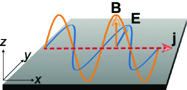
Figure 1: Schematic of the two-dimensional system under consideration. An electric field $\mathbf{E}$ in the plane and a magnetic field $\mathbf{B}$ perpendicular to the plane are applied. The induced Hall current $\mathbf{j}$ is perpendicular to the direction of the electric field. The fields propagate in the same direction as the Hall current.

In this Letter, we consider a two-dimensional clean system and apply an in-plane electric field polarized along $y$-direction and propagating along $x$-direction, i.e. $\mathbf{E}=E_{y}\hat{y}e^{iqx-i\omega t}$+c.c., and a magnetic field polarized along $z$-direction, i.e. $\mathbf{B}=B_{z}\hat{z}e^{iqx-i\omega t}$+c.c., as illustrated in Fig. 1. Here, $q$ and $\omega$ are the moduli of the momentum and frequency of the fields, respectively. Under the presence of such external fields, the system can be described by the vector potential

$$\mathbf{A}=A_{y}\hat{y}e^{iqx-i\omega t}+\mathrm{c.c.},$$ (2)

where $A_{y}$ satisfies the relations $A_{y}=E_{y}/i\omega=B_{z}/iq$.

In this paper, we consider a generic linear continuum Hamiltonian targeting various two-dimensional Dirac systems in the limit of the low temperature. Then, the corresponding Hamiltonian of the sample $H_{0}(\mathbf{k})$ satisfies the restriction $\partial_{k_{i}}\partial_{k_{j}}H_{0}(\mathbf{k})=\partial_{k_{i}}\hat{v}_{j}=0$, where $\hat{v}_{j}=\partial_{k_{j}}H_{0}(\mathbf{k})$ is the velocity operator in $j$-direction and we have set $\hbar=1$. As a result, the full Hamiltonian of the system in the presence of the external fields can be written as $H(\mathbf{k})=H_{0}(\mathbf{k})+H^{{}^{\prime}}(\mathbf{k})$. Here $H^{{}^{\prime}}(\mathbf{k})$ is the perturbed Hamiltonian , which is given by

$$H^{{}^{\prime}}(\mathbf{k})=e\hat{\mathbf{v}}\cdot\mathbf{A},$$ (3)

where $-e$ is the charge of the electron. The second-order term of the vector potential in the perturbed Hamiltonian, i.e. $e^{2}\partial_{\mathbf{k}}(\mathbf{v}\cdot\mathbf{A})\cdot\mathbf{A}/2$, vanishes in the linear system.

Second-order nonlinear response theory Now we consider the second-order response with respect to the vector potential. The current operator in our system is described by $\hat{j}_{x}=-e\partial_{k_{x}}H(\mathbf{k})=-e\hat{v}_{x}$. By using Fourier transformation and second quantization, the expectation value of the current $\langle\hat{j}_{x}(2\mathbf{q},2i\omega)\rangle$ in momentum-frequency space can be written as Araki et al. (2021)

$$j_{x}(2\mathbf{q},2i\omega)=\frac{1}{S\beta}\sum_{\mathbf{k},i\omega_{n}}\mathrm{Tr}[\hat{j}_{x}\delta G(\mathbf{k},i\omega_{n};\mathbf{k}-2\mathbf{q},i\omega_{n}-2i\omega)],$$ (4)

where $S$ is the area of the system, $\beta=1/k_{B}T$ is the inverse temperature, $\mathbf{q}=q\hat{x}$, $\omega_{n}=(2n+1)\pi/\beta$ and $\omega=2m\pi/\beta$ are the fermionic and bosonic Matsubara frequencies, respectively. For second-order response, the perturbation of the Green function is given by

$$\delta G(\mathbf{k},i\omega_{n};\mathbf{k}-2\mathbf{q},i\omega_{n}-2i\omega)=e^{2}G(\mathbf{k},i\omega_{n})\hat{v}_{y}A_{y}G(\mathbf{k}-\mathbf{q},i\omega_{n}-i\omega)\hat{v}_{y}A_{y}G(\mathbf{k}-2\mathbf{q},i\omega_{n}-2i\omega),$$ (5)

where the Green function has the form

$$G(\mathbf{k},i\omega_{n})=\sum_{a}\frac{|u_{a}(\mathbf{k})\rangle\langle u_{a}(\mathbf{k})|}{i\omega_{n}+\mu-\varepsilon_{a}(\mathbf{k})}.$$ (6)

Here $|u_{a}(\mathbf{k})\rangle$ is the periodic part of Bloch wave functions for band $a$, $\mu$ is the chemical potential, and $\varepsilon_{a}(\mathbf{k})$ is the energy dispersion of band $a$. For linear Hamiltonian, the second-order nonlinear response forms a triangle diagram, as shown in Fig. 2. Unlike the previous treatment of the second-order response Gao et al. (2020); Parker et al. (2019), here the momentum $\mathbf{q}$ of the external fields is taken into account.

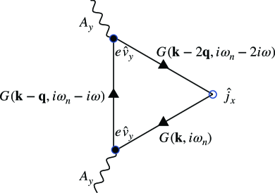
Figure 2: The triangle diagram of the second-order response current. The wavy lines refer to the external vector potential, the solid lines are the electron propagator, i.e., the Green function, the solid vertexes represent the operator $e\hat{v}_{y}$ in the perturbed Hamiltonian, and the hollow vertex denotes the Hall current operator.

By taking the Matsubara sum over $i\omega_{n}$ in Eq. (4) and performing the analytical continuation $i\omega\rightarrow\omega+i0$, one obtains

$$j_{x}(2\mathbf{q},2\omega)=\frac{-e^{3}}{S}\Pi(\mathbf{q},\omega)A_{y}A_{y},$$ (7)

with

$$\Pi(\mathbf{q},\omega)=\sum_{\mathbf{k},a,b,c}M_{abc}(\mathbf{k},\mathbf{q})F_{abc}(\mathbf{k},\mathbf{q},\omega).$$ (8)

Here

$$M_{abc}(\mathbf{k},\mathbf{q}) = \langle u_{c}(\mathbf{k}-2\mathbf{q})|\hat{v}_{x}|u_{a}(\mathbf{k})\rangle\langle u_{a}(\mathbf{k})|\hat{v}_{y}|u_{b}(\mathbf{k}-\mathbf{q})\rangle$$ (9)

$$\times\langle u_{b}(\mathbf{k}-\mathbf{q})|\hat{v}_{y}|u_{c}(\mathbf{k}-2\mathbf{q})\rangle$$

is the correlation function with band indices $a$, $b$, and $c$,

$$F_{abc}(\mathbf{k},\mathbf{q},\omega)=\frac{1}{\varepsilon_{a}(\mathbf{k})-\varepsilon_{b}(\mathbf{k}-\mathbf{q})-\omega}\bigg{[}\frac{f(\varepsilon_{a}(\mathbf{k}))-f(\varepsilon_{c}(\mathbf{k}-2\mathbf{q}))}{\varepsilon_{a}(\mathbf{k})-\varepsilon_{c}(\mathbf{k}-2\mathbf{q})-2\omega}-\frac{f(\varepsilon_{b}(\mathbf{k}-\mathbf{q}))-f(\varepsilon_{c}(\mathbf{k}-2\mathbf{q}))}{\varepsilon_{b}(\mathbf{k}-\mathbf{q})-\varepsilon_{c}(\mathbf{k}-2\mathbf{q})-\omega}\bigg{]}$$ (10)

is the Matsubara summation, and $f(\varepsilon_{i}(\mathbf{k}))=1/(e^{\beta(\varepsilon_{i}(\mathbf{k})-\mu)}+1)$ is the Fermi-Dirac distribution function.

To derive the response to the electric and magnetic fields, we need to expand $\Pi(\mathbf{q},\omega)$ to first order in $q$ as $\Pi(\mathbf{q},\omega)=\Pi(0,\omega)+q\Pi(\omega)$, where $\Pi(\omega)=\partial_{q}\Pi(\mathbf{q},\omega)|_{q=0}$. Then we expand $\Pi(\omega)$ in terms of $\omega$ to zero-order, i.e. $\Pi(\omega)=\Pi(0)=\mathrm{lim}_{\omega\rightarrow 0}\Pi(\omega)$. As a result, $\Pi(\mathbf{q},\omega)A_{y}$ in Eq. (7) becomes $-i\Pi(0)B_{z}$. Here we actually take the uniform limit, i.e. sending $\mathbf{q}\rightarrow 0$ before $\omega\rightarrow 0$. The function $\Pi(\mathbf{q},\omega)$ satisfies the following relation SI

$$\Pi(\mathbf{q},\omega)=\Pi^{*}(-\mathbf{q},-\omega).$$ (11)

Then one can get

$$\Pi(0)=-\Pi^{*}(0)=i\mathrm{lm}\Pi(0).$$ (12)

The current thus becomes

$$j_{x}(2\omega)=\frac{ie^{3}}{S\omega}\mathrm{lm}\Pi(0)E_{y}B_{z}.$$ (13)

For two-band system, the energy bands $a,b,c$ in $M_{abc}(\mathbf{k},\mathbf{q})$ and $F_{abc}(\mathbf{k},\mathbf{q},\omega)$ can only be upper or lower bands. If the bands $a,b,c$ are the same band, $\mathrm{lm}M_{aaa}(\mathbf{k},0)$ and $F_{aaa}(\mathbf{k},0,\omega)$ will all be zero. Then $\mathrm{lm}\Pi(\omega)=\partial_{q}\mathrm{lm}M_{aaa}(\mathbf{k},\mathbf{q})|_{q=0}F_{aaa}(\mathbf{k},0,\omega)+\mathrm{lm}M_{aaa}(\mathbf{k},0)\partial_{q}F_{aaa}(\mathbf{k},\mathbf{q},\omega)|_{q=0}=0$, i.e. the full intraband term’s contribution to the second-order response vanishes. Note that for the linear response in the uniform limit, the intra-band terms also give zero contributions Chang and Yang (2015); Zhong et al. (2016). For nonzero response, the bands $a,b,c$ should take $a,b,b$; $a,b,a$; $a,a,b$.

One can decompose $\Pi(\mathbf{q},\omega)$ in Eq. (8) into the intraband part $\Pi_{\mathrm{intra}}(\mathbf{q},\omega)$ and interband part $\Pi_{\mathrm{inter}}(\mathbf{q},\omega)$. The intraband part $\Pi_{\mathrm{intra}}(\mathbf{q},\omega)$ is further split into three terms such that $\Pi_{\mathrm{intra}}(\mathbf{q},\omega)=\sum_{\alpha=1}^{3}\Pi^{(\alpha)}_{\mathrm{intra}}(\mathbf{q},\omega)$, where

$$\Pi^{(1)}_{\mathrm{intra}}(\mathbf{q},\omega)=\sum_{\mathbf{k},a\neq b}\frac{-M_{abb}(\mathbf{k},\mathbf{q})}{\varepsilon^{\mathbf{0},\mathbf{q}}_{a,b}(\mathbf{k})-\omega}\frac{f^{\mathbf{q},2\mathbf{q}}_{b,b}(\mathbf{k})}{\varepsilon^{\mathbf{q},2\mathbf{q}}_{b,b}(\mathbf{k})-\omega},$$ (14)

$$\Pi^{(2)}_{\mathrm{intra}}(\mathbf{q},\omega)=\sum_{\mathbf{k},a\neq b}\frac{M_{aba}(\mathbf{k},\mathbf{q})}{\varepsilon^{\mathbf{0},\mathbf{q}}_{a,b}(\mathbf{k})-\omega}\frac{f^{\mathbf{0},2\mathbf{q}}_{a,a}(\mathbf{k})}{\varepsilon^{\mathbf{0},2\mathbf{q}}_{a,a}(\mathbf{k})-2\omega},$$ (15)

and

$$\Pi^{(3)}_{\mathrm{intra}}(\mathbf{q},\omega)=\sum_{\mathbf{k},a\neq b}\frac{M_{aab}(\mathbf{k},\mathbf{q})}{\varepsilon^{\mathbf{q},2\mathbf{q}}_{a,b}(\mathbf{k})-\omega}\frac{f^{\mathbf{0},\mathbf{q}}_{a,a}(\mathbf{k})}{\varepsilon^{\mathbf{0},\mathbf{q}}_{a,a}(\mathbf{k})-\omega},$$ (16)

Here we use the abbreviations $f^{\mathbf{q},\mathbf{q^{\prime}}}_{a,b}(\mathbf{k})=f(\varepsilon_{a}(\mathbf{k}-\mathbf{q}))-f(\varepsilon_{b}(\mathbf{k}-\mathbf{q^{\prime}}))$ and $\varepsilon^{\mathbf{q},\mathbf{q^{\prime}}}_{a,b}(\mathbf{k})=\varepsilon_{a}(\mathbf{k}-\mathbf{q})-\varepsilon_{b}(\mathbf{k}-\mathbf{q^{\prime}})$. From these, we expand the imaginary part of $\Pi_{\mathrm{intra}}(\mathbf{q},\omega)$, take the uniform limit and obtain SI

$$\mathrm{lm}\Pi_{\mathrm{intra}}(0)=-\sum_{\mathbf{k},a\neq b}F^{ab}_{xy}v_{ay}\partial_{k_{x}}f(\varepsilon_{a}(\mathbf{k})),$$ (17)

where $F^{ab}_{xy}=-2\mathrm{lm}\langle\partial_{k_{x}}u_{a}(\mathbf{k})|u_{b}(\mathbf{k})\rangle\langle u_{b}(\mathbf{k})|\partial_{k_{y}}u_{a}(\mathbf{k})\rangle$ is the Berry curvature which is the imaginary part of quantum geometric tensor Provost and Vallee (1980); Zhang (2022) and $v_{iy}=\partial_{k_{y}}\varepsilon_{i}(\mathbf{k})$ is the band velocity along $y$-axis.

The interband part $\Pi_{\mathrm{inter}}(\mathbf{q},\omega)$ is also composed of three terms such that $\Pi_{\mathrm{inter}}(\mathbf{q},\omega)=\sum_{\alpha=1}^{3}\Pi^{(\alpha)}_{\mathrm{inter}}(\mathbf{q},\omega)$. Since the interband term is irrespective of the order of limits $\mathbf{q}\rightarrow 0$ and $\omega\rightarrow 0$, we take $\omega=0$ before $\mathbf{q}\rightarrow 0$ and have

$$\Pi^{(1)}_{\mathrm{inter}}(\mathbf{q},0)=\sum_{\mathbf{k},a\neq b}\frac{M_{abb}(\mathbf{k},\mathbf{q})}{\varepsilon^{\mathbf{0},\mathbf{q}}_{a,b}(\mathbf{k})}\frac{f^{\mathbf{0},2\mathbf{q}}_{a,b}(\mathbf{k})}{\varepsilon^{\mathbf{0},2\mathbf{q}}_{a,b}(\mathbf{k})},$$ (18)

$$\Pi^{(2)}_{\mathrm{inter}}(\mathbf{q},0)=-\sum_{\mathbf{k},a\neq b}\frac{M_{aba}(\mathbf{k},\mathbf{q})}{\varepsilon^{\mathbf{0},\mathbf{q}}_{a,b}(\mathbf{k})}\frac{f^{2\mathbf{q},\mathbf{q}}_{a,b}(\mathbf{k})}{\varepsilon^{2\mathbf{q},\mathbf{q}}_{a,b}(\mathbf{k})},$$ (19)

and

$$\Pi^{(3)}_{\mathrm{inter}}(\mathbf{q},0)=-\sum_{\mathbf{k},a\neq b}\frac{M_{aab}(\mathbf{k},\mathbf{q})}{\varepsilon^{\mathbf{q},2\mathbf{q}}_{a,b}(\mathbf{k})}\frac{f^{\mathbf{0},2\mathbf{q}}_{a,b}(\mathbf{k})}{\varepsilon^{\mathbf{0},2\mathbf{q}}_{a,b}(\mathbf{k})}.$$ (20)

From these, we expand $\mathrm{lm}\Pi_{\mathrm{inter}}(\mathbf{q},0)$ and get SI

$$\mathrm{lm}\Pi_{\mathrm{inter}}(0)=\sum_{\mathbf{k},a\neq b}f(\varepsilon_{a}(\mathbf{k}))\partial_{k_{x}}\big{[}F^{ab}_{xy}(v_{ay}-v_{by})\big{]}.$$ (21)

Combining the contribution of the intraband and interband terms, the Hall current becomes

$$j_{x}(2\omega)=\frac{ie^{3}}{S\omega}\sum_{\mathbf{k},a\neq b}f(\varepsilon_{a}(\mathbf{k}))\partial_{k_{x}}\big{[}F^{ab}_{xy}(2v_{ay}-v_{by})\big{]}E_{y}B_{z}.$$ (22)

Here we have taken integration by parts for the Fermi surface term in Eq. (17). Eq. (22) is the main result of this paper. It shows that in the Hall device, there is a second-order Hall response which is proportional to a dipole, i.e.

$$D=\int\frac{d^{2}k}{(2\pi)^{2}}\sum_{a\neq b}f(\varepsilon_{a}(\mathbf{k}))\partial_{k_{x}}\big{[}F^{ab}_{xy}(2v_{ay}-v_{by})\big{]}.$$ (23)

Under time-reversal symmetry, such a dipole vanishes, since the partial differential, the Berry curvature, and the band velocity are all odd functions of momentum in such a case. It is worth noting that there is a similar second-order response to the electromagnetic field, i.e. the magnetononlinear anomalous Hall effect Gao et al. (2014). However, this effect comes from the intrinsic mechanism of the band structure, has time-reversal symmetry, and has no Drude-like dependency on $\omega\tau$. Here for our clean system, the relaxation time $\tau$ approaches infinity.

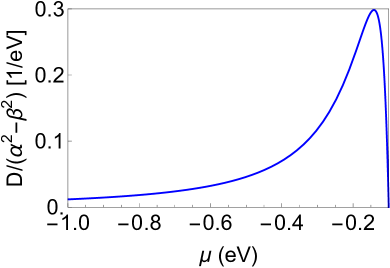
Figure 3: The dipole as a function of chemical potential $\mu$. The band gap $\Delta$ is chosen to be 0.1eV.

Massive Dirac model As an example, let us consider a Dirac Hamiltonian with broken time-reversal symmetry motivated by the LaAlO₃/LaNiO₃/LaAlO₃ quantum well system with spin-orbit coupling Tao and Tsymbal (2018). The low-energy physics of the material around Dirac points can be described by the Hamiltonian

$$H_{0}(\mathbf{k})=\alpha(k_{x}-k_{y})\sigma_{x}+\beta(k_{x}+k_{y})\sigma_{z}+\Delta\sigma_{y}.$$ (24)

Here $\mathbf{k}$ is momentum defined near the Dirac point, $(\alpha,\beta)$ are expansion coefficients determined by the band parameters. The gap $\Delta$ is generated by turning on the spin-orbit coupling. The energy dispersion of upper band $(+)$ and lower band $(-)$ are respectively given by $\varepsilon_{\pm}(\mathbf{k})=\pm\varepsilon_{0}$, where $\varepsilon_{0}=\sqrt{k^{{}^{\prime}2}_{x}+k^{{}^{\prime}2}_{y}+\Delta^{2}}$, $k^{{}^{\prime}}_{x}=\alpha(k_{x}-k_{y})$, and $k^{{}^{\prime}}_{y}=\beta(k_{x}+k_{y})$. Then the band velocity is $v_{\pm y}=\pm(-\alpha k^{{}^{\prime}}_{x}+\beta k^{{}^{\prime}}_{y})/\varepsilon_{0}$ and the Berry curvature is given by $F^{-+}_{xy}=-\alpha\beta\Delta/\varepsilon_{0}^{3}$. In the case of zero temperature and the chemical potential $\mu<-\Delta$, the integrand function in the dipole, i.e. Eq. (23), becomes $3\alpha\beta\Delta[k^{{}^{\prime}2}_{x}(3\alpha^{2}+\beta^{2})-k^{{}^{\prime}2}_{y}(\alpha^{2}+3\beta^{2})+\Delta^{2}(\beta^{2}-\alpha^{2})]/(4\pi^{2}\varepsilon_{0}^{6})$, $dk_{x}dk_{y}=dk^{{}^{\prime}}_{x}dk^{{}^{\prime}}_{y}/(2\alpha\beta)$, and the integral is over the region $\varepsilon_{-}(\mathbf{k})<\mu$, i.e. $k^{{}^{\prime}2}_{x}+k^{{}^{\prime}2}_{y}>\mu^{2}-\Delta^{2}$. By using polar coordinate, the dipole is found to be

$$D=\frac{3(\alpha^{2}-\beta^{2})(\mu^{2}-\Delta^{2})\Delta}{8\pi\mu^{4}}.$$ (25)

At the chemical potential $\mu=-\sqrt{2}\Delta$, the dipole takes its maximum $D=3(\alpha^{2}-\beta^{2})/(32\pi\Delta)$, which is shown in Fig. 3.

Discussion Here we mainly restrict our system to be linear. If we relax the restriction, the perturbed Hamiltonian and Hall current operator can contain second-order and first-order terms of vector potential $\mathbf{A}$, respectively. As a consequence, in addition to the considered triangle term, two additional terms will appear in the second-response current.

Up to the second order of the electric and magnetic fields, the total Hall current in time-reversal breaking materials can be expressed in the form $j_{x}=\sigma_{xy}E_{y}+\gamma_{xij}E_{i}E_{j}+\alpha_{xij}E_{i}B_{j}$. Note that the first two terms do not depend on the frequency of the external fields. Therefore, the dipole in this nonlinear electromagnetic response can be extracted from the derivative of the current with respect to the oscillation period of the external fields.

In this work, we consider the two-dimensional system where electric and magnetic fields are placed as shown in Fig. 1. Following a similar method, the results can be generalized to a three-dimensional system where electric and magnetic fields are placed in other ways. Besides, by replacing the Hall current operator in the response with the spin current operator, the research can be extended to the spin system too Sinova et al. (2004); Zhang and Rhim (2022).

Acknowledgements A.Z. and J.-W.R. were supported by the National Research Foundation of Korea (NRF) Grant funded by the Korea government (MSIT) (Grant No. 2021R1A2C1010572). J.-W.R. was supported by the National Research Foundation of Korea (NRF) Grant funded by the Korea government (MSIT) (Grant No. 2021R1A5A1032996) and Creation of the Quantum Information Science R&D Ecosystem (Grant No. 2022M3H3A106307411) through the National Research Foundation of Korea (NRF) funded by the Korean government (Ministry of Science and ICT).

Supplementary Materials for
“Nonlinear electromagnetic response for Hall effect in time-reversal breaking materials”

I I. The proof of the relation: $\Pi(\mathbf{q},\omega)=\Pi^{*}(-\mathbf{q},-\omega)$

Here we show the details of the proof of the relation: $\Pi(\mathbf{q},\omega)=\Pi^{*}(-\mathbf{q},-\omega)$ in the main text, i.e.

$$\sum_{\mathbf{k},a,b,c}M_{abc}(\mathbf{k},\mathbf{q})F_{abc}(\mathbf{k},\mathbf{q},\omega)=\sum_{\mathbf{k},a,b,c}M^{*}_{abc}(\mathbf{k},-\mathbf{q})F_{abc}(\mathbf{k},-\mathbf{q},-\omega).$$ (S1)

We start from the expressions of $M_{abc}(\mathbf{k},\mathbf{q})$ and $F_{abc}(\mathbf{k},\mathbf{q},\omega)$, i.e.

$$M_{abc}(\mathbf{k},\mathbf{q})=\langle u_{c}(\mathbf{k}-2\mathbf{q})|\hat{v}_{x}|u_{a}(\mathbf{k})\rangle\langle u_{a}(\mathbf{k})|\hat{v}_{y}|u_{b}(\mathbf{k}-\mathbf{q})\rangle\langle u_{b}(\mathbf{k}-\mathbf{q})|\hat{v}_{y}|u_{c}(\mathbf{k}-2\mathbf{q})\rangle$$ (S2)

and

$$F_{abc}(\mathbf{k},\mathbf{q},\omega)=\frac{1}{\varepsilon_{a}(\mathbf{k})-\varepsilon_{b}(\mathbf{k}-\mathbf{q})-\omega}\bigg{[}\frac{f(\varepsilon_{a}(\mathbf{k}))-f(\varepsilon_{c}(\mathbf{k}-2\mathbf{q}))}{\varepsilon_{a}(\mathbf{k})-\varepsilon_{c}(\mathbf{k}-2\mathbf{q})-2\omega}-\frac{f(\varepsilon_{b}(\mathbf{k}-\mathbf{q}))-f(\varepsilon_{c}(\mathbf{k}-2\mathbf{q}))}{\varepsilon_{b}(\mathbf{k}-\mathbf{q})-\varepsilon_{c}(\mathbf{k}-2\mathbf{q})-\omega}\bigg{]}.$$ (S3)

Then $M^{*}_{abc}(\mathbf{k},-\mathbf{q})$ is

$$M^{*}_{abc}(\mathbf{k},-\mathbf{q})=\langle u_{a}(\mathbf{k})|\hat{v}_{x}|u_{c}(\mathbf{k}+2\mathbf{q})\rangle\langle u_{c}(\mathbf{k}+2\mathbf{q})|\hat{v}_{y}|u_{b}(\mathbf{k}+\mathbf{q})\rangle\langle u_{b}(\mathbf{k}+\mathbf{q})|\hat{v}_{y}|u_{a}(\mathbf{k})\rangle,$$ (S4)

and $F^{*}_{abc}(\mathbf{k},-\mathbf{q},-\omega)$ becomes

$$F_{abc}(\mathbf{k},-\mathbf{q},-\omega)=\frac{1}{\varepsilon_{a}(\mathbf{k})-\varepsilon_{b}(\mathbf{k}+\mathbf{q})+\omega}\bigg{[}\frac{f(\varepsilon_{a}(\mathbf{k}))-f(\varepsilon_{c}(\mathbf{k}+2\mathbf{q}))}{\varepsilon_{a}(\mathbf{k})-\varepsilon_{c}(\mathbf{k}+2\mathbf{q})+2\omega}-\frac{f(\varepsilon_{b}(\mathbf{k}+\mathbf{q}))-f(\varepsilon_{c}(\mathbf{k}+2\mathbf{q}))}{\varepsilon_{b}(\mathbf{k}+\mathbf{q})-\varepsilon_{c}(\mathbf{k}+2\mathbf{q})+\omega}\bigg{]}.$$ (S5)

Transferring the momentum from $\mathbf{k}$ to $\mathbf{k}-2\mathbf{q}$, $\sum_{\mathbf{k},a,b,c}M^{*}_{abc}(\mathbf{k},-\mathbf{q})F_{abc}(\mathbf{k},-\mathbf{q},-\omega)$ will be $\sum_{\mathbf{k},a,b,c}M^{*}_{abc}(\mathbf{k}-2\mathbf{q},-\mathbf{q})F_{abc}(\mathbf{k}-2\mathbf{q},-\mathbf{q},-\omega)$, where

$$M^{*}_{abc}(\mathbf{k}-2\mathbf{q},-\mathbf{q})=\langle u_{a}(\mathbf{k}-2\mathbf{q})|\hat{v}_{x}|u_{c}(\mathbf{k})\rangle\langle u_{c}(\mathbf{k})|\hat{v}_{y}|u_{b}(\mathbf{k}-\mathbf{q})\rangle\langle u_{b}(\mathbf{k}-\mathbf{q})|\hat{v}_{y}|u_{a}(\mathbf{k}-2\mathbf{q})\rangle,$$ (S6)

and

$$F_{abc}(\mathbf{k}-2\mathbf{q},-\mathbf{q},-\omega) = \frac{1}{\varepsilon_{a}(\mathbf{k}-2\mathbf{q})-\varepsilon_{b}(\mathbf{k}-\mathbf{q})+\omega}$$ (S7)

$$\bigg{[}\frac{f(\varepsilon_{a}(\mathbf{k}-2\mathbf{q}))-f(\varepsilon_{c}(\mathbf{k}))}{\varepsilon_{a}(\mathbf{k}-2\mathbf{q})-\varepsilon_{c}(\mathbf{k})+2\omega}-\frac{f(\varepsilon_{b}(\mathbf{k}-\mathbf{q}))-f(\varepsilon_{c}(\mathbf{k}))}{\varepsilon_{b}(\mathbf{k}-\mathbf{q})-\varepsilon_{c}(\mathbf{k})+\omega}\bigg{]}.$$

Now exchanging the indexes $a$ and $c$, i.e. $a\leftrightarrow c$, one gets $\sum_{\mathbf{k},a,b,c}M^{*}_{cba}(\mathbf{k}-2\mathbf{q},-\mathbf{q})F_{cba}(\mathbf{k}-2\mathbf{q},-\mathbf{q},-\omega)$, where

$$M^{*}_{cba}(\mathbf{k}-2\mathbf{q},-\mathbf{q})=\langle u_{c}(\mathbf{k}-2\mathbf{q})|\hat{v}_{x}|u_{a}(\mathbf{k})\rangle\langle u_{a}(\mathbf{k})|\hat{v}_{y}|u_{b}(\mathbf{k}-\mathbf{q})\rangle\langle u_{b}(\mathbf{k}-\mathbf{q})|\hat{v}_{y}|u_{c}(\mathbf{k}-2\mathbf{q})\rangle=M_{abc}(\mathbf{q}),$$ (S8)

and

$$F_{cba}(\mathbf{k}-2\mathbf{q},-\mathbf{q},-\omega) = \frac{1}{\varepsilon_{c}(\mathbf{k}-2\mathbf{q})-\varepsilon_{b}(\mathbf{k}-\mathbf{q})+\omega}$$ (S9)

$$\bigg{[}\frac{f(\varepsilon_{c}(\mathbf{k}-2\mathbf{q}))-f(\varepsilon_{a}(\mathbf{k}))}{\varepsilon_{c}(\mathbf{k}-2\mathbf{q})-\varepsilon_{a}(\mathbf{k})+2\omega}-\frac{f(\varepsilon_{b}(\mathbf{k}-\mathbf{q}))-f(\varepsilon_{a}(\mathbf{k}))}{\varepsilon_{b}(\mathbf{k}-\mathbf{q})-\varepsilon_{a}(\mathbf{k})+\omega}\bigg{]}$$

$$= F_{abc}(\mathbf{q},\omega).$$

Thus we have

$$\sum_{\mathbf{k},a,b,c}M^{*}_{abc}(-\mathbf{q})F_{abc}(-\mathbf{q},-\omega)=\sum_{\mathbf{k},a,b,c}M_{abc}(\mathbf{q})F_{abc}(\mathbf{q},\omega),$$ (S10)

i.e. the (S1) is proved.

II II. The contribution of the intraband terms

Here we show the contribution of the intraband terms in $\Pi(\mathbf{q},\omega)$. The intraband terms in $\Pi(\mathbf{q},\omega)$ are respectively

$$\Pi^{(1)}_{\mathrm{intra}}(\mathbf{q},\omega)=\sum_{\mathbf{k},a\neq b}\frac{-M_{abb}(\mathbf{k},\mathbf{q})}{\varepsilon_{a}(\mathbf{k})-\varepsilon_{b}(\mathbf{k}-\mathbf{q})-\omega}\frac{f(\varepsilon_{b}(\mathbf{k}-\mathbf{q}))-f(\varepsilon_{b}(\mathbf{k}-2\mathbf{q}))}{\varepsilon_{b}(\mathbf{k}-\mathbf{q})-\varepsilon_{b}(\mathbf{k}-2\mathbf{q})-\omega},$$ (S11)

$$\Pi^{(2)}_{\mathrm{intra}}(\mathbf{q},\omega)=\sum_{\mathbf{k},a\neq b}\frac{M_{aba}(\mathbf{k},\mathbf{q})}{\varepsilon_{a}(\mathbf{k})-\varepsilon_{b}(\mathbf{k}-\mathbf{q})-\omega}\frac{f(\varepsilon_{a}(\mathbf{k}))-f(\varepsilon_{a}(\mathbf{k}-2\mathbf{q}))}{\varepsilon_{a}(\mathbf{k})-\varepsilon_{a}(\mathbf{k}-2\mathbf{q})-2\omega},$$ (S12)

and

$$\Pi^{(3)}_{\mathrm{intra}}(\mathbf{q},\omega)=\sum_{\mathbf{k},a\neq b}\frac{M_{aab}(\mathbf{k},\mathbf{q})}{\varepsilon_{a}(\mathbf{k}-\mathbf{q})-\varepsilon_{b}(\mathbf{k}-2\mathbf{q})-\omega}\frac{f(\varepsilon_{a}(\mathbf{k}))-f(\varepsilon_{a}(\mathbf{k}-\mathbf{q}))}{\varepsilon_{a}(\mathbf{k})-\varepsilon_{a}(\mathbf{k}-\mathbf{q})-\omega}.$$ (S13)

Expanding these intraband terms to first order in $q$, one can get

$$\Pi^{(1)}_{\mathrm{intra}}(\mathbf{q},\omega)=q\sum_{\mathbf{k},a\neq b}\frac{M_{abb}(\mathbf{k},0)}{\varepsilon_{a}(\mathbf{k})-\varepsilon_{b}(\mathbf{k})-\omega}\frac{f^{\prime}(\varepsilon_{b}(\mathbf{k}))}{\omega},$$ (S14)

$$\Pi^{(2)}_{\mathrm{intra}}(\mathbf{q},\omega)=-q\sum_{\mathbf{k},a\neq b}\frac{M_{aba}(\mathbf{k},0)}{\varepsilon_{a}(\mathbf{k})-\varepsilon_{b}(\mathbf{k})-\omega}\frac{f^{\prime}(\varepsilon_{a}(\mathbf{k}))}{\omega},$$ (S15)

and

$$\Pi^{(3)}_{\mathrm{intra}}(\mathbf{q},\omega)=-q\sum_{\mathbf{k},a\neq b}\frac{M_{aab}(\mathbf{k},0)}{\varepsilon_{a}(\mathbf{k})-\varepsilon_{b}(\mathbf{k})-\omega}\frac{f^{\prime}(\varepsilon_{a}(\mathbf{k}))}{\omega}.$$ (S16)

Here $f^{\prime}=\partial_{k_{x}}f$. We note that $M_{aba}(\mathbf{k},0)=\langle u_{a}(\mathbf{k})|\hat{v}_{x}|u_{a}(\mathbf{k})\rangle\langle u_{a}(\mathbf{k})|\hat{v}_{y}|u_{b}(\mathbf{k})\rangle\langle u_{b}(\mathbf{k})|\hat{v}_{y}|u_{a}(\mathbf{k})\rangle$ which is a real number, so $\Pi^{(2)}_{\mathrm{intra}}(\mathbf{q},\omega)$ can be omitted since it does not contribute to the response. Besides, after exchanging the indexes $a,b$ for $\Pi^{(1)}_{\mathrm{intra}}(\mathbf{q},\omega)$, one has

$$\Pi^{(1)}_{\mathrm{intra}}(\mathbf{q},\omega) = -q\sum_{\mathbf{k},a\neq b}\frac{M_{baa}(\mathbf{k},0)}{\varepsilon_{a}(\mathbf{k})-\varepsilon_{b}(\mathbf{k})+\omega}\frac{f^{\prime}(\varepsilon_{a}(\mathbf{k}))}{\omega}$$ (S17)

$$= q\sum_{\mathbf{k},a\neq b}\frac{M_{baa}(\mathbf{k},0)f^{\prime}(\varepsilon_{a}(\mathbf{k}))}{\varepsilon_{a}(\mathbf{k})-\varepsilon_{b}(\mathbf{k})}\bigg{(}\frac{1}{\varepsilon_{a}(\mathbf{k})-\varepsilon_{b}(\mathbf{k})}-\frac{1}{\omega}\bigg{)},$$

where

$$M_{baa}(\mathbf{k},0)=\langle u_{a}(\mathbf{k})|\hat{v}_{x}|u_{b}(\mathbf{k})\rangle\langle u_{b}(\mathbf{k})|\hat{v}_{y}|u_{a}(\mathbf{k})\rangle\langle u_{a}(\mathbf{k})|\hat{v}_{y}|u_{a}(\mathbf{k})\rangle,$$ (S18)

and we have expanded $\Pi^{(1)}_{\mathrm{intra}}(\mathbf{q},\omega)$ in the limit $\omega\rightarrow 0$. Note that $M_{aab}(\mathbf{k},0)$ in $\Pi^{(3)}_{\mathrm{intra}}(\mathbf{q},\omega)$ is

$$M_{aab}(\mathbf{k},0) = \langle u_{b}(\mathbf{k})|\hat{v}_{x}|u_{a}(\mathbf{k})\rangle\langle u_{a}(\mathbf{k})|\hat{v}_{y}|u_{a}(\mathbf{k})\rangle\langle u_{a}(\mathbf{k})|\hat{v}_{y}|u_{b}(\mathbf{k})\rangle$$ (S19)

$$= M^{*}_{baa}(\mathbf{k},0).$$

Thus

$$\Pi^{(3)}_{\mathrm{intra}}(\mathbf{q},\omega)=-q\sum_{\mathbf{k},a\neq b}\frac{M^{*}_{baa}(\mathbf{k},0)f^{\prime}(\varepsilon_{a}(\mathbf{k}))}{\varepsilon_{a}(\mathbf{k})-\varepsilon_{b}(\mathbf{k})}\bigg{(}\frac{1}{\varepsilon_{a}(\mathbf{k})-\varepsilon_{b}(\mathbf{k})}+\frac{1}{\omega}\bigg{)},$$ (S20)

and then

$$\mathrm{lm}\Pi_{\mathrm{intra}}(\mathbf{q},\omega)=2q\sum_{\mathbf{k},a\neq b}\frac{\mathrm{lm}M_{baa}(\mathbf{k},0)f^{\prime}(\varepsilon_{a}(\mathbf{k}))}{(\varepsilon_{a}(\mathbf{k})-\varepsilon_{b}(\mathbf{k}))^{2}}=-q\sum_{\mathbf{k},a\neq b}F^{ab}_{xy}v_{ay}\partial_{k_{x}}f(\varepsilon_{a}(\mathbf{k})),$$ (S21)

i.e. the intraband terms in $\Pi(\mathbf{q},\omega)$ contributes $-\sum_{\mathbf{k},a\neq b}F^{ab}_{xy}v_{ay}\partial_{k_{x}}f(\varepsilon_{a}(\mathbf{k}))$ to $\mathrm{lm}\Pi(0)$. Here $F^{ab}_{xy}=-2\mathrm{lm}\langle u_{a}(\mathbf{k})|\hat{v}_{x}|u_{b}(\mathbf{k})\rangle\langle u_{b}(\mathbf{k})|\hat{v}_{y}|u_{a}(\mathbf{k})\rangle/(\varepsilon_{a}(\mathbf{k})-\varepsilon_{b}(\mathbf{k}))^{2}$ is the Berry curvature.

III III. The contribution of the interband terms

Here we show the derivation of Eq. (21) in the main text. The interband terms in $\Pi(\mathbf{q},\omega)$ can be respectively decomposed as

$$\sum_{\mathbf{k},a\neq b}\frac{M_{abb}(\mathbf{k},\mathbf{q})}{\varepsilon_{a}(\mathbf{k})-\varepsilon_{b}(\mathbf{k}-\mathbf{q})}\frac{f(\varepsilon_{a}(\mathbf{k}))-f(\varepsilon_{b}(\mathbf{k}-2\mathbf{q}))}{\varepsilon_{a}(\mathbf{k})-\varepsilon_{b}(\mathbf{k}-2\mathbf{q})}$$

$$=\sum_{\mathbf{k},a\neq b}\frac{M_{abb}(\mathbf{k},\mathbf{q})}{\varepsilon_{a}(\mathbf{k})-\varepsilon_{b}(\mathbf{k}-\mathbf{q})}\frac{f(\varepsilon_{a}(\mathbf{k}))}{\varepsilon_{a}(\mathbf{k})-\varepsilon_{b}(\mathbf{k}-2\mathbf{q})}$$

$$-\sum_{\mathbf{k},a\neq b}\frac{M_{baa}(\mathbf{k},\mathbf{q})}{\varepsilon_{a}(\mathbf{k}-\mathbf{q})-\varepsilon_{b}(\mathbf{k})}\frac{f(\varepsilon_{a}(\mathbf{k}-2\mathbf{q}))}{\varepsilon_{a}(\mathbf{k}-2\mathbf{q})-\varepsilon_{b}(\mathbf{k})},$$ (S22)

$$\sum_{\mathbf{k},a\neq b}\frac{-M_{aba}(\mathbf{k},\mathbf{q})}{\varepsilon_{a}(\mathbf{k})-\varepsilon_{b}(\mathbf{k}-\mathbf{q})}\frac{f(\varepsilon_{a}(\mathbf{k}-2\mathbf{q}))-f(\varepsilon_{b}(\mathbf{k}-\mathbf{q}))}{\varepsilon_{a}(\mathbf{k}-2\mathbf{q})-\varepsilon_{b}(\mathbf{k}-\mathbf{q})}$$

$$=\sum_{\mathbf{k},a\neq b}\frac{-M_{aba}(\mathbf{k},\mathbf{q})}{\varepsilon_{a}(\mathbf{k})-\varepsilon_{b}(\mathbf{k}-\mathbf{q})}\frac{f(\varepsilon_{a}(\mathbf{k}-2\mathbf{q}))}{\varepsilon_{a}(\mathbf{k}-2\mathbf{q})-\varepsilon_{b}(\mathbf{k}-\mathbf{q})}$$

$$+\sum_{\mathbf{k},a\neq b}\frac{M_{bab}(\mathbf{k},\mathbf{q})}{\varepsilon_{a}(\mathbf{k}-\mathbf{q})-\varepsilon_{b}(\mathbf{k})}\frac{f(\varepsilon_{a}(\mathbf{k}-\mathbf{q}))}{\varepsilon_{a}(\mathbf{k}-\mathbf{q})-\varepsilon_{b}(\mathbf{k}-2\mathbf{q})},$$ (S23)

and

$$\sum_{\mathbf{k},a\neq b}\frac{-M_{aab}(\mathbf{k},\mathbf{q})}{\varepsilon_{a}(\mathbf{k}-\mathbf{q})-\varepsilon_{b}(\mathbf{k}-2\mathbf{q})}\frac{f(\varepsilon_{a}(\mathbf{k}))-f(\varepsilon_{b}(\mathbf{k}-2\mathbf{q}))}{\varepsilon_{a}(\mathbf{k})-\varepsilon_{b}(\mathbf{k}-2\mathbf{q})}$$

$$=\sum_{\mathbf{k},a\neq b}\frac{-M_{aab}(\mathbf{k},\mathbf{q})}{\varepsilon_{a}(\mathbf{k}-\mathbf{q})-\varepsilon_{b}(\mathbf{k}-2\mathbf{q})}\frac{f(\varepsilon_{a}(\mathbf{k}))}{\varepsilon_{a}(\mathbf{k})-\varepsilon_{b}(\mathbf{k}-2\mathbf{q})}$$

$$+\sum_{\mathbf{k},a\neq b}\frac{M_{bba}(\mathbf{k},\mathbf{q})}{\varepsilon_{a}(\mathbf{k}-2\mathbf{q})-\varepsilon_{b}(\mathbf{k}-\mathbf{q})}\frac{f(\varepsilon_{a}(\mathbf{k}-2\mathbf{q}))}{\varepsilon_{a}(\mathbf{k}-2\mathbf{q})-\varepsilon_{b}(\mathbf{k})}.$$ (S24)

We note that $M_{abb}(\mathbf{k},\mathbf{q})=\langle u_{b}(\mathbf{k}-2\mathbf{q})|\hat{v}_{x}|u_{a}(\mathbf{k})\rangle\langle u_{a}(\mathbf{k})|\hat{v}_{y}|u_{b}(\mathbf{k}-\mathbf{q})\rangle\langle u_{b}(\mathbf{k}-\mathbf{q})|\hat{v}_{y}|u_{b}(\mathbf{k}-2\mathbf{q})\rangle$ can be expanded as

$$M_{abb}(\mathbf{k},\mathbf{q})=M_{abb}(\mathbf{k},0)+q\partial_{q}M_{abb}(\mathbf{k},\mathbf{q})|_{q=0},$$ (S25)

where $M_{abb}(\mathbf{k},0)=\langle u_{a}(\mathbf{k})|\hat{v}_{y}|u_{b}(\mathbf{k})\rangle\langle u_{b}(\mathbf{k})|\hat{v}_{x}|u_{a}(\mathbf{k})\rangle v_{by}$, and

$$\partial_{q}M_{abb}(\mathbf{k},\mathbf{q})|_{q=0} = -\partial_{k_{x}}M_{abb}(\mathbf{k},0)-\langle\partial_{k_{x}}u_{b}(\mathbf{k})|u_{a}(\mathbf{k})\rangle\langle u_{a}(\mathbf{k})|\hat{v}_{y}|u_{b}(\mathbf{k})\rangle v_{ax}v_{by}$$ (S26)

$$-\langle u_{b}(\mathbf{k})|\hat{v}_{x}|u_{a}(\mathbf{k})\rangle\langle u_{a}(\mathbf{k})|\hat{v}_{y}|u_{b}(\mathbf{k})\rangle\langle u_{b}(\mathbf{k})|\hat{v}_{y}|u_{a}(\mathbf{k})\rangle\langle u_{a}(\mathbf{k})|\partial_{k_{x}}u_{b}(\mathbf{k})\rangle$$

$$+\langle u_{b}(\mathbf{k})|\partial_{k_{x}}u_{a}(\mathbf{k})\rangle\langle u_{a}(\mathbf{k})|\hat{v}_{y}|u_{b}(\mathbf{k})\rangle v_{bx}v_{by}$$

$$+\langle u_{b}(\mathbf{k})|\hat{v}_{x}|u_{a}(\mathbf{k})\rangle\langle\partial_{k_{x}}u_{a}(\mathbf{k})|u_{b}(\mathbf{k})\rangle v_{by}v_{by}$$

$$= -\partial_{k_{x}}M_{abb}(\mathbf{k},0)-\langle\partial_{k_{x}}u_{a}(\mathbf{k})|u_{b}(\mathbf{k})\rangle\langle u_{b}(\mathbf{k})|\hat{v}_{y}|u_{a}(\mathbf{k})\rangle(v_{ax}+v_{bx})v_{by}.$$

Here $v_{ai}=\partial_{k_{i}}\varepsilon_{a}(\mathbf{k})$, and we have omitted real terms. Besides,

$$\frac{1}{\varepsilon_{a}(\mathbf{k})-\varepsilon_{b}(\mathbf{k}-\mathbf{q})}\frac{f(\varepsilon_{a}(\mathbf{k}))}{\varepsilon_{a}(\mathbf{k})-\varepsilon_{b}(\mathbf{k}-2\mathbf{q})} = \bigg{[}\frac{1}{(\varepsilon_{a}(\mathbf{k})-\varepsilon_{b}(\mathbf{k}))^{2}}-3q\frac{v_{bx}}{(\varepsilon_{a}(\mathbf{k})-\varepsilon_{b}(\mathbf{k}))^{3}}\bigg{]}f(\varepsilon_{a}(\mathbf{k})).$$

So the first term of Eq. (III) contributes

$$\sum_{\mathbf{k},a\neq b}\mathrm{lm}\bigg{[}\frac{\partial_{q}M_{abb}(\mathbf{k},\mathbf{q})|_{q=0}}{(\varepsilon_{a}(\mathbf{k})-\varepsilon_{b}(\mathbf{k}))^{2}}-3\frac{M_{abb}(\mathbf{k},0)v_{bx}}{(\varepsilon_{a}(\mathbf{k})-\varepsilon_{b}(\mathbf{k}))^{3}}\bigg{]}f(\varepsilon_{a}(\mathbf{k})$$ (S28)

to the $\mathrm{lm}\Pi(0)$ in the current.

The second term of Eq. (III) can be rewritten as

$$-\sum_{\mathbf{k},a\neq b}\frac{M_{baa}(\mathbf{k},\mathbf{q})}{\varepsilon_{a}(\mathbf{k}-\mathbf{q})-\varepsilon_{b}(\mathbf{k})}\frac{f(\varepsilon_{a}(\mathbf{k}-2\mathbf{q}))}{\varepsilon_{a}(\mathbf{k}-2\mathbf{q})-\varepsilon_{b}(\mathbf{k})}=-\sum_{\mathbf{k},a\neq b}\frac{M_{baa}(\mathbf{k}+2\mathbf{q},\mathbf{q})}{\varepsilon_{a}(\mathbf{k}+\mathbf{q})-\varepsilon_{b}(\mathbf{k}+2\mathbf{q})}\frac{f(\varepsilon_{a}(\mathbf{k}))}{\varepsilon_{a}(\mathbf{k})-\varepsilon_{b}(\mathbf{k}+2\mathbf{q})}.$$ (S29)

Here $M_{baa}(\mathbf{k}+2\mathbf{q},\mathbf{q})=\langle u_{a}(\mathbf{k})|\hat{v}_{x}|u_{b}(\mathbf{k}+2\mathbf{q})\rangle\langle u_{b}(\mathbf{k}+2\mathbf{q})|\hat{v}_{y}|u_{a}(\mathbf{k}+\mathbf{q})\rangle\langle u_{a}(\mathbf{k}+\mathbf{q})|\hat{v}_{y}|u_{a}(\mathbf{k})\rangle$ can be decomposed as

$$M_{baa}(\mathbf{k}+2\mathbf{q},\mathbf{q}) = M_{baa}(\mathbf{k},0)+q\partial_{q}M_{baa}(\mathbf{k}+2\mathbf{q},\mathbf{q})|_{q=0}$$ (S30)

with $M_{baa}(\mathbf{k},0)=\langle u_{a}(\mathbf{k})|\hat{v}_{x}|u_{b}(\mathbf{k})\rangle\langle u_{b}(\mathbf{k})|\hat{v}_{y}|u_{a}(\mathbf{k})\rangle v_{ay}$ and

$$\partial_{q}M_{baa}(\mathbf{k}+2\mathbf{q},\mathbf{q})|_{q=0} = \partial_{k_{x}}M_{baa}(\mathbf{k},0)-\langle\partial_{k_{x}}u_{a}(\mathbf{k})|u_{b}(\mathbf{k})\rangle\langle u_{b}(\mathbf{k})\hat{v}_{y}|u_{a}(\mathbf{k})\rangle(v_{ax}+v_{bx})v_{ay}.$$

Besides,

$$\frac{-1}{\varepsilon_{a}(\mathbf{k}+\mathbf{q})-\varepsilon_{b}(\mathbf{k}+2\mathbf{q})}\frac{f(\varepsilon_{a}(\mathbf{k}))}{\varepsilon_{a}(\mathbf{k})-\varepsilon_{b}(\mathbf{k}+2\mathbf{q})}=\bigg{[}\frac{-1}{(\varepsilon_{a}(\mathbf{k})-\varepsilon_{b}(\mathbf{k}))^{2}}+q\frac{v_{ax}-4v_{bx}}{(\varepsilon_{a}(\mathbf{k})-\varepsilon_{b}(\mathbf{k}))^{3}}\bigg{]}f(\varepsilon_{a}(\mathbf{k})).$$ (S32)

So the second term of Eq. (III) contributes

$$\sum_{\mathbf{k},a\neq b}\mathrm{lm}\bigg{[}\frac{-\partial_{q}M_{baa}(\mathbf{k}+2\mathbf{q},\mathbf{q})|_{q=0}}{(\varepsilon_{a}(\mathbf{k})-\varepsilon_{b}(\mathbf{k}))^{2}}+\frac{M_{baa}(\mathbf{k},0)(v_{ax}-4v_{bx})}{(\varepsilon_{a}(\mathbf{k})-\varepsilon_{b}(\mathbf{k}))^{3}}\bigg{]}f(\varepsilon_{a}(\mathbf{k}))$$ (S33)

to the $\mathrm{lm}\Pi(0)$ in the current.

Similarly, for the terms in Eqs. (III) and (III), the contribution to the $\mathrm{lm}\Pi(0)$ are respectively

$$\sum_{\mathbf{k},a\neq b}\mathrm{lm}\bigg{[}\frac{-\partial_{q}M_{aba}(\mathbf{k}+2\mathbf{q},\mathbf{q})|_{q=0}}{(\varepsilon_{a}(\mathbf{k})-\varepsilon_{b}(\mathbf{k}))^{2}}+2\frac{M_{aba}(\mathbf{k},0)(v_{ax}-v_{bx})}{(\varepsilon_{a}(\mathbf{k})-\varepsilon_{b}(\mathbf{k}))^{3}}\bigg{]}f(\varepsilon_{a}(\mathbf{k})),$$ (S34)

$$\sum_{\mathbf{k},a\neq b}\mathrm{lm}\bigg{[}\frac{\partial_{q}M_{bab}(\mathbf{k}+\mathbf{q},\mathbf{q})|_{q=0}}{(\varepsilon_{a}(\mathbf{k})-\varepsilon_{b}(\mathbf{k}))^{2}}\bigg{]}f(\varepsilon_{a}(\mathbf{k})),$$ (S35)

$$\sum_{\mathbf{k},a\neq b}\mathrm{lm}\bigg{[}\frac{-\partial_{q}M_{aab}(\mathbf{k},\mathbf{q})|_{q=0}}{(\varepsilon_{a}(\mathbf{k})-\varepsilon_{b}(\mathbf{k}))^{2}}-\frac{M_{aab}(\mathbf{k},0)(v_{ax}-4v_{bx})}{(\varepsilon_{a}(\mathbf{k})-\varepsilon_{b}(\mathbf{k}))^{3}}\bigg{]}f(\varepsilon_{a}(\mathbf{k})),$$ (S36)

and

$$\sum_{\mathbf{k},a\neq b}\mathrm{lm}\bigg{[}\frac{\partial_{q}M_{bba}(\mathbf{k}+2\mathbf{q},\mathbf{q})|_{q=0}}{(\varepsilon_{a}(\mathbf{k})-\varepsilon_{b}(\mathbf{k}))^{2}}+3\frac{M_{bba}(\mathbf{k},0)v_{bx}}{(\varepsilon_{a}(\mathbf{k})-\varepsilon_{b}(\mathbf{k}))^{3}}\bigg{]}f(\varepsilon_{a}(\mathbf{k})),$$ (S37)

where

$$M_{aba}(\mathbf{k},0)=\langle u_{a}(\mathbf{k})|\hat{v}_{y}|u_{b}(\mathbf{k})\rangle\langle u_{b}(\mathbf{k})|\hat{v}_{y}|u_{a}(\mathbf{k})\rangle v_{ax}---real,discarded,$$ (S38)

$$\partial_{q}M_{aba}(\mathbf{k}+2\mathbf{q},\mathbf{q})|_{q=0}=2\langle\partial_{k_{x}}u_{a}(\mathbf{k})|u_{b}(\mathbf{k})\rangle\langle u_{b}(\mathbf{k})|\hat{v}_{y}|u_{a}(\mathbf{k})\rangle v_{ax}v_{by},$$ (S39)

$$\partial_{q}M_{bab}(\mathbf{k}+\mathbf{q},\mathbf{q})|_{q=0}=2\langle\partial_{k_{x}}u_{a}(\mathbf{k})|u_{b}(\mathbf{k})\rangle\langle u_{b}(\mathbf{k})|\hat{v}_{y}|u_{a}(\mathbf{k})\rangle v_{bx}v_{ay},$$ (S40)

$$M_{aab}(\mathbf{k},0)=\langle u_{a}(\mathbf{k})|\hat{v}_{y}|u_{b}(\mathbf{k})\rangle\langle u_{b}(\mathbf{k})|\hat{v}_{x}|u_{a}(\mathbf{k})\rangle v_{ay},$$ (S41)

$$\partial_{q}M_{aab}(\mathbf{k},\mathbf{q})|_{q=0}=-\partial_{k_{x}}M_{aab}(\mathbf{k},0)-\langle\partial_{k_{x}}u_{a}(\mathbf{k})|u_{b}(\mathbf{k})\rangle\langle u_{b}(\mathbf{k})|\hat{v}_{y}|u_{a}(\mathbf{k})\rangle(v_{ax}+v_{bx})v_{ay},$$ (S42)

$$M_{bba}(\mathbf{k},0)=\langle u_{a}(\mathbf{k})|\hat{v}_{x}|u_{b}(\mathbf{k})\rangle\langle u_{b}(\mathbf{k})|\hat{v}_{y}|u_{a}(\mathbf{k})\rangle v_{by},$$ (S43)

$$\partial_{q}M_{bba}(\mathbf{k}+2\mathbf{q},\mathbf{q})|_{q=0}=\partial_{k_{x}}M_{bba}(\mathbf{k},0)-\langle\partial_{k_{x}}u_{a}(\mathbf{k})|u_{b}(\mathbf{k})\rangle\langle u_{b}(\mathbf{k})|\hat{v}_{y}|u_{a}(\mathbf{k})\rangle(v_{ax}+v_{bx})v_{by}.$$ (S44)

Sum the terms in Eqs. (S28), (S33), (S34), (S35), (S36), and (S37) up, one obtains

$$\mathrm{lm}\Pi(0) = \sum_{\mathbf{k},a\neq b}f(\varepsilon_{a}(\mathbf{k}))\bigg{\{}\frac{2\partial_{k_{x}}\big{[}\mathrm{lm}\langle u_{a}(\mathbf{k})|\hat{v}_{x}|u_{b}(\mathbf{k})\rangle\langle u_{b}(\mathbf{k})|\hat{v}_{y}|u_{a}(\mathbf{k})\rangle(v_{by}-v_{ay})\big{]}}{(\varepsilon_{a}(\mathbf{k})-\varepsilon_{b}(\mathbf{k}))^{2}}$$ (S45)

$$+\frac{4\mathrm{lm}\langle u_{a}(\mathbf{k})|\hat{v}_{x}|u_{b}(\mathbf{k})\rangle\langle u_{b}(\mathbf{k})|\hat{v}_{y}|u_{a}(\mathbf{k})\rangle(v_{ax}-v_{bx})(v_{ay}-v_{by})}{(\varepsilon_{a}(\mathbf{k})-\varepsilon_{b}(\mathbf{k}))^{3}}\bigg{\}}$$

$$= \sum_{\mathbf{k},a\neq b}f(\varepsilon_{a}(\mathbf{k}))\partial_{k_{x}}\big{[}F^{ab}_{xy}(v_{ay}-v_{by})\big{]}.$$

Thus Eq. (21) in the main text is derived.

References

• Hall et al. (1879) E. H. Hall et al., American Journal of Mathematics 2, 287 (1879).
• Klitzing et al. (1980) K. v. Klitzing, G. Dorda,  and M. Pepper, Physical review letters 45, 494 (1980).
• Girvin and Prange (1990) S. Girvin and R. Prange, The quantum Hall effect (Springer-Verlag, New York, 1990).
• Yoshioka (2002) D. Yoshioka, The quantum Hall effect, Vol. 133 (Springer Science & Business Media, 2002).
• Thouless et al. (1982) D. J. Thouless, M. Kohmoto, M. P. Nightingale,  and M. den Nijs, Physical review letters 49, 405 (1982).
• Haldane (1988) F. D. M. Haldane, Physical review letters 61, 2015 (1988).
• Kane and Mele (2005) C. L. Kane and E. J. Mele, Physical review letters 95, 146802 (2005).
• Hasan and Kane (2010) M. Z. Hasan and C. L. Kane, Reviews of modern physics 82, 3045 (2010).
• Qi and Zhang (2011) X.-L. Qi and S.-C. Zhang, Reviews of Modern Physics 83, 1057 (2011).
• Yan and Felser (2017) B. Yan and C. Felser, Annual Review of Condensed Matter Physics 8, 337 (2017).
• Armitage et al. (2018) N. Armitage, E. Mele,  and A. Vishwanath, Reviews of Modern Physics 90, 015001 (2018).
• Tsirkin and Souza (2022) S. Tsirkin and I. Souza, SciPost Physics Core 5, 039 (2022).
• Holder et al. (2020) T. Holder, D. Kaplan,  and B. Yan, Physical Review Research 2, 033100 (2020).
• Watanabe and Yanase (2021) H. Watanabe and Y. Yanase, Physical Review X 11, 011001 (2021).
• Gao et al. (2014) Y. Gao, S. A. Yang,  and Q. Niu, Physical review letters 112, 166601 (2014).
• Liu et al. (2021) H. Liu, J. Zhao, Y.-X. Huang, W. Wu, X.-L. Sheng, C. Xiao,  and S. A. Yang, Physical Review Letters 127, 277202 (2021).
• Wang et al. (2021) C. Wang, Y. Gao,  and D. Xiao, Physical Review Letters 127, 277201 (2021).
• Sodemann and Fu (2015) I. Sodemann and L. Fu, Physical review letters 115, 216806 (2015).
• Morimoto et al. (2016) T. Morimoto, S. Zhong, J. Orenstein,  and J. E. Moore, Physical Review B 94, 245121 (2016).
• Facio et al. (2018) J. I. Facio, D. Efremov, K. Koepernik, J.-S. You, I. Sodemann,  and J. Van Den Brink, Physical review letters 121, 246403 (2018).
• You et al. (2018) J.-S. You, S. Fang, S.-Y. Xu, E. Kaxiras,  and T. Low, Physical Review B 98, 121109 (2018).
• Zhang et al. (2018) Y. Zhang, Y. Sun,  and B. Yan, Physical Review B 97, 041101 (2018).
• Ma et al. (2019) Q. Ma, S.-Y. Xu, H. Shen, D. MacNeill, V. Fatemi, T.-R. Chang, A. M. Mier Valdivia, S. Wu, Z. Du, C.-H. Hsu, et al., Nature 565, 337 (2019).
• Kang et al. (2019) K. Kang, T. Li, E. Sohn, J. Shan,  and K. F. Mak, Nature materials 18, 324 (2019).
• Gao et al. (2020) Y. Gao, F. Zhang,  and W. Zhang, Physical Review B 102, 245116 (2020).
• Du et al. (2021a) Z. Du, C. Wang, H.-P. Sun, H.-Z. Lu,  and X. Xie, Nature communications 12, 1 (2021a).
• Du et al. (2021b) Z. Du, H.-Z. Lu,  and X. Xie, Nature Reviews Physics 3, 744 (2021b).
• Araki et al. (2021) Y. Araki, D. Suenaga, K. Suzuki,  and S. Yasui, Physical Review Research 3, 023098 (2021).
• Parker et al. (2019) D. E. Parker, T. Morimoto, J. Orenstein,  and J. E. Moore, Physical Review B 99, 045121 (2019).
• (30) See Supplemental Material for (i) the proof of the Eq. (11), (ii) the derivation of the Eq. (17), and (iii) the derivation of the Eq. (21) in the main text .
• Chang and Yang (2015) M.-C. Chang and M.-F. Yang, Physical Review B 91, 115203 (2015).
• Zhong et al. (2016) S. Zhong, J. E. Moore,  and I. Souza, Physical review letters 116, 077201 (2016).
• Provost and Vallee (1980) J. Provost and G. Vallee, Communications in Mathematical Physics 76, 289 (1980).
• Zhang (2022) A. Zhang, Chinese Physics B 31, 040201 (2022).
• Tao and Tsymbal (2018) L. Tao and E. Y. Tsymbal, Physical Review B 98, 121102 (2018).
• Sinova et al. (2004) J. Sinova, D. Culcer, Q. Niu, N. Sinitsyn, T. Jungwirth,  and A. H. MacDonald, Physical review letters 92, 126603 (2004).
• Zhang and Rhim (2022) A. Zhang and J.-W. Rhim, Communications Physics 5, 195 (2022).