Unified Software Design Patterns for Simulated Annealing

Abstract

Any optimization algorithm programming interface can be seen as a black-box function with additional free parameters. In this spirit, simulated annealing (SA) can be implemented in pseudo-code within the dimensions of a single slide with free parameters relating to the annealing schedule. Such an implementation, however, necessarily neglects much of the structure necessary to take advantage of advances in computing resources and algorithmic breakthroughs. Simulated annealing is often introduced in myriad disciplines, from discrete examples like the Traveling Salesman Problem (TSP) to molecular cluster potential energy exploration or even explorations of a protein’s configurational space. Theoretical guarantees also demand a stricter structure in terms of statistical quantities, which cannot simply be left to the user. We will introduce several standard paradigms and demonstrate how these can be "lifted" into a unified framework using object-oriented programming in Python. We demonstrate how clean, interoperable, reproducible programming libraries can be used to access and rapidly iterate on variants of Simulated Annealing in a manner which can be extended to serve as a best practices blueprint or design pattern for a data-driven optimization library.

Keywords global optimization, algorithms, high performance computing, software design, metaheuristics

1 Introduction

For an optimization problem in any discipline, from finding optimal catalysts [1] to obtaining parameters for fitting coefficients for heat transfer equations from experimental data [2] to finding nucleation rates [3], being able to locate saddle points and minima are of crucial interest. The objective function used across various disciplines [4, 5, 6, 7, 8] varies widely in continuity, complexity, and dimensionality which contributes to direct search methods being infeasible despite advances in computational resources. Simulated Annealing (SA) was first described by Kirkpatrick et al. [9], building on ideas from computational statistical mechanics [10]. It is one of a class of stochastic algorithms for optimization problems, especially well-suited to finding global extrema, which draws inspiration from the metallurgical concept of annealing wherein a material is heated and cooled slowly in a controlled manner to relax its structure. Essentially, the highest ordered state corresponds to the to the lowest entropy configuration, which is also the energy minima, pictorially depicted at a molecular level in Fig. 1. Since the algorithm is often formulated in terms of a “stopping criteria” and applied to NP-hard problems, i.e., those which cannot be solved in polynomial time, it is also known as a heuristic [11, 12].

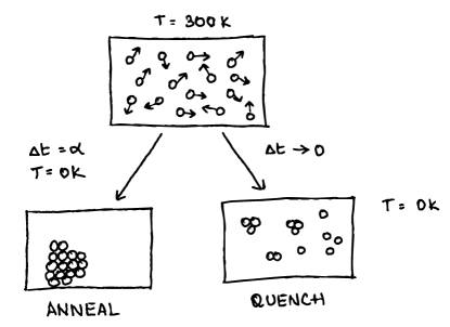
Figure 1: Quenching and annealing at a molecular level. (T=300K) Shows a system at a finite temperature. (T=0K, QUENCH) shows the effect (“flash freezing”) of quenching. (T=0K, ANNEAL) demonstrates the effect (“slow cooling”) of annealing. By entropic arguments, at the same temperature, the disordered (quenched) structure has more energy than the ordered structure.

In its most naive representation, following the intuition of slow cooling to prevent quenching, the SA algorithm is derivative-free, and takes only the objective function, with a cooling schedule, and can be represented as [13, 14]:

Data: $S_{init}$, $F_{obj}$, $F_{T}$

Result: $S_{sol}$

$S_{cur}\leftarrow S_{init}$;

foreach $timestep\in[1,\infty]$ do

       $Ti\leftarrow F_{T}(t)$;

       if $T_{i}=0$ then

            return $S_{cur}$

       end if

      $S_{try}\leftarrow F_{obj}(S_{rand})$;

       $\Delta E\leftarrow F_{obj}(S_{cur})-F_{obj}(S_{try})$;

       if $\Delta E<0$ then

            $S_{cur}\leftarrow S_{try}$

      else

             $S_{cur}\leftarrow S_{try}$with probability $e^{-\Delta E/Ti}$;

            

       end if

      

end foreach

Algorithm 1 Naive Simulated Annealing, with states generated by a $F_{obj}$ and temperatures from a cooling schedule $F_{T}$

A naive approach, as outlined in Alg. 1 essentially outlines a random start-based hill-climbing, with the inclusion of a possibility of having moves that do not lead to a higher value of the fitness function. This is the intuitive reasoning behind why SA outperforms direct search, especially in higher dimensions, where the possibility of being stuck in a local minimum is much higher and harder to evade, given the geometry of measures in high-dimensional spaces [15].

However, several concerns from the literature [16, 17, 18] are immediately relevant; the algorithm samples the neighborhood at random, explicitly rejects multiple steps, and has no immediate extension for (HPC) systems. Additionally, given the physical connections, it would be best to have the theory mirrored (to the point of possibly accepting a domain-specific language, or DSL) closely within the code [19, 20]. However, the algorithm demonstrates no openings for incorporating the theory of Markov Chain Monte Carlo (MCMC) sampling theory or statistical mechanics (two driving theoretical pillars of SA).

The past four decades have yielded many insights [21, 18, 22] into the theoretical underpinnings of the algorithm, its convergence [23], and extensions [24, 25]. Yet SA is often taught and implemented in a naive or restricted fashion [17], sometimes even being implemented so poorly as to require complete removal, as in the Scientific Python scipy code-base. In other cases, established recipes and implementations [26] can even propagate logical fallacies about the algorithm and its applicability (e.g., to continuous problems) itself. This is doubly concerning in the era of reproducible results and responsible computing [27, 28, 29, 30]. Despite the rise of exa-scale [31] computing, and advances in sampling methods [32, 24], modular software design [33, 20, 19], research software engineering [34], and packaging [35, 36, 37]; poor design of SA routines has persisted.

Part of the problem is a proliferation of competing nomenclature for modifications in the general SA framework; changes in different sampling methods, equilibrium distributions, and evaluation points are reported as new methods, including (FSA) [38], (GSA) [39], . We will demonstrate their provenance and uncover the appropriate abstraction to implement each one in a unified programming framework.

The remainder of this chapter is structured as follows. We briefly cover, the necessary theoretical background needed to critically examine the requirements of a modern, object-oriented SA implementation, followed by an exposition on some of the existing library APIs. We will then demonstrate the building blocks of a modern, coherent, implementation of SA, which is amenable to extension and exposes an API which is rich enough to encode all algorithmic variants and problem-specific parameters in a domain-agnostic manner.

2 Theoretical Background

Let us define the basic elements needed for a slightly more formal understanding of the components of the SA algorithm [41].

Definition 2.1.

A real-valued function $F$ defined over a finite set $S$

This leads to the understanding that $F_{S}$ is a current solution point (which also opens the possibility of constraints). To complete the minimal structure for the algorithm Alg. 1, we further define a neighborhood, and assume that $S^{*}\subset S$ is the set of global minima.

Definition 2.2.

For each $i\in S$, the set $S(i)\subset S-{i}$ is the set of neighbors of $i$ or the neighborhood

At this point, given a function, evaluating neighboring solutions and storing the values will eventually hit upon the global minimum, and this is essentially the concept behind brute-force optimization methods. Adding a stochastic term to the sampling of points would technically result in a rather pointless stochastic optimizer. Instead, we will connect the system to a random process (in time) with a finite number of possible states by defining rates of transitioning to the neighborhood points.

Definition 2.3.

$\forall i\in S$ we have positive coefficients such that $q_{ij},j\in S(i)$ with $\sum_{j\in S(i)}q_{ij}=1$

We further assume that the $j\in S(i)$ if and only if $i\in S(j)$, which will essentially ensure that only neighbors can transition among each other.

Finally, we introduced two more definitions to connect to the physical concept of annealing. One is trivial, we define; (without thermodynamical considerations) a value associated with the $N^{th}$ step of the algorithm to be the temperature; that is, if we use the concept of “time” for each step, we have a temperature at each time. The other corresponds to the “controlled” cooling in the annealing process.

Definition 2.4.

The cooling schedule is $T:N\to(0,\infty)$ where $T$ is a non-increasing function, and $T(t)$ is the temperature

By construction, we have established that the SA algorithm can be interpreted as a discrete-time inhomogeneous Markov chain $x(t)$, where the Markovian property of each successive step depending only on the previous value, is not immediately evident in the algorithm. However, recall that the dynamics of a Markov chain can be encoded in the transition probabilities defined in the Metropolis algorithm such that [17]:

$$M_{i,j}=\begin{cases}0,&\text{if}\ i\notin S(j)\\ \frac{1}{N_{j}},&\text{if}\ F_{S_{i}}\geq F_{S_{j}}\\ \exp{\left(\frac{-\Delta F_{S}/T}{N_{j}}\right)},&\text{if}\ F_{S_{i}}\leq F_{S_{j}}\\ 1-\sum_{k\neq j}M_{k,j},&\text{if}\ i=j\end{cases}$$ (1)

Where $N_{j}$ is the number of neighboring states to $j$, or the size of the neighborhood. From this explicit formulation, we note that the algorithm is necessarily bound by temperatures corresponding to all moves being accepted (at infinite temperature) and when no moves are accepted (zero temperature).

Already, we have equipped Alg. 1 with more theoretical structure and considerations than are originally evident from the interpretation of “local search” with randomization.

From a Markov chain dynamics perspective, we would prefer to simulate an irreducible (i.e., one where every state is accessible, a.k.a an ergodic chain) and aperiodic (so there is no backtracking) chain which has a target density and which is point mass at the global minimum. As this is not feasible for all but toy problems, the key idea in SA is to have a homogeneous Markov chain $x_{T}(t)$ at each step when the temperature is held constant. If additionally, $q_{ij}=q_{ji}$, then by $x_{T}(t)$ is also reversible and so, by either statistical mechanical arguments [42] or the detailed balance conditions or the entropy maximization principles of states [18], we obtain a stationary target density which is the Boltzmann-Gibbs distribution (which is why SA in this form is also called the Boltzmann Simulated Annealing algorithm, BSA).

$$\pi_{T}(i)=\frac{1}{Z_{T}}\exp\left[-\frac{J(i)}{T}\right],\quad i\in S$$ (2)

SA is best described and interpreted in the language of statistical mechanics [17], where $Z_{T}$ is the partition function. However, we can neglect this interpretation and take it to be only a normalizing coefficient. Instead, we will enumerate the most common variants and continue designing a code-base for the same.

We will note, however, that not all variations are theoretically guaranteed to reach the global minimum [18], which (for Boltzmann SA) has sufficiency conditions for ergodic search, which can be expressed in the form of a cooling schedule such that:

$$T_{k}=T_{0}\frac{\ln{k_{0}}}{\ln{k}}$$ (3)

2.1 Exemplary Variants

Two out of the plethora of SA variants, stand out as representatives of algorithms which enable simplifying implementations. As a rule of thumb, any abstraction will lead to general (and often simpler) code, while specific instances can easily be tested in an automated manner. Note that we do not consider auxiliary information, e.g., adding mode-following methods, [43], which can lead to approaches akin to basin hopping [44] or global search methods based on long time scale dynamics [45].

2.1.1 Fast Simulated Annealing (FSA)

Szu et. al. [38] designed a modification of SA by replacing the neighbor selection with a distribution of move sizes (or visiting distribution) which allows long jumps in state space. The cooling schedule is applied to a transformed parameter $T_{gen}$, which parametrizes a Cauchy distribution, $P(x)=\pi^{-1}T_{gen}(T_{gen}^{2}+x^{2})^{-1}$ while the Metropolis acceptance is based on a Fermi equilibrium distribution instead of the Boltzmann.

2.1.2 Generalized Simulated Annealing (GSA)

Tsallis et. al. [39] demonstrated that the Boltzmann SA and Cauchy SA can be generalized using Tsallis statistics using a distorted Cauchy-Lorentz visiting distribution and a shape parameter $q_{v}$ [46, 17, 47].

$$P(x)\propto T_{q_{v}}(t)^{\frac{D}{3-q_{v}}}\times\left(1+\frac{(q_{v}-1)\Delta x^{2}}{[T_{qv}(t)]^{2/(3-q_{v})}}\right)^{(q_{v}-1)^{-1}+(D-1)/2}$$ (4)

Where the cooling rate is:

$$T_{q_{v}}(t)=T_{q_{v}}(0)\times\frac{2^{q_{v}-1}-1}{(1+t)^{q_{v}-1}-1}$$ (5)

Along with a generalized Metropolis algorithm using a free parameter $Q_{a}$

$$P_{Q_{a}}=\begin{cases}\min{(1,[1-(1-Q_{a})\beta\Delta F_{S}]^{\frac{1}{1-Q_{a}}})},&\text{if}\ Q_{a}\geq 1\\ 0,&\text{if}\ Q_{a}<1\text{and}\ [1-(1-Q_{a})\beta\Delta F_{S}]<0\end{cases}$$ (6)

Importantly, from an implementation perspective:

$q_{v}=1,Q_{a}=1$

Boltzmann Simulated Annealing

$q_{v}=2,Q_{a}=1$

Cauchy / Fast Simulated Annealing

2.2 Control knobs

We will focus on continuous or discrete optimization problems which use floating point values, that is, we do not explicitly consider integral constraints or combinatorial formulations. For such problems, we have the following elements of the algorithm which may be parameterized [17, 14, 18]:

Move classes

The neighbor selection methodology, e.g., the Metropolis algorithm, Eqn. 1 as shown in Alg. 1

Cooling schedules

The change in temperature at each step, e.g., Eqn. 3, Eqn. 5

Repetitions

This quantifies the time spent in each iteration (change in temperature) and is often calculated by feedback, but variations exist, Table

Stopping Criteria

The final termination condition or by a user-defined relative tolerance

Target / Equilibrium distributions

Changing the target distribution from the Boltzmann to the Fermi distribution

Acceptance criteria

The Metropolis algorithm is essentially a choice of neighbor followed by an acceptance criterion, though modifications of this can change the equilibrium distribution

Any reasonable code-base must be flexible enough to accommodate changes to and tests of any of these control knobs, and we will demonstrate such a design in subsequent sections. A good implementation in a structured hierarchy should also be able to reproduce up-to machine precision, the predictions for which a GSA reduces to FSA and BSA.

2.3 Markov Chain Monte Carlo Perspective

An alternate formulation of the SA algorithm can be developed from a different perspective. At any fixed temperature $T$, the probability of being in a particular state $X$ with a corresponding function $F_{X}$ we have:

$$P(X)\sim\exp{(-F_{X})/T}$$ (7)

Equation 7 implies that a Markov chain with its target distribution set to this state probability will spend an overwhelming amount of time at the function minima, while the temperature controls the amount by which the chain will “explore” the landscape. At each stage, the temperature is lowered, thus progressively reaching towards the highest concentration of the probability density, which will be the global minimum or minima.

For a first approximation to demonstrate this approach, consider the Metropolis-Hastings algorithm for a target density $f$ and (proposal) density $q$, which will produce a Markov chain with an acceptance criteria [48] for each newly proposed state given by:

$$p(x,y)=\mathrm{min}\left\{\frac{f(y)}{f(x)}\frac{q(x|y)}{q(y|x)},1\right\}$$ (8)

This means that a standard SA algorithm can now be expressed as a series of Metropolis-Hastings samplers, one for each temperature. This frees the user from setting inner-loop iterations, which are needed in many SA formulations, and additionally makes the algorithm amenable to trivial parallelization. For each temperature, multiple chains can be simulated, and their mixing will give an indication of when to terminate the sampling. Several existing chain diagnostics can be used for the same, including the Gelman-Rubin statistic [49] or effective sample size [48], a measure of how many samples are drawn from the “true” distribution.

There are some drawbacks to this formulation as well. The samplers may not be constrained based on clipping values to the edge of the domain as this will lead to artificially inflated acceptance values and the distribution will not be explored properly.

3 Programming Considerations

Equipped with the basic theoretical grounding, we are now in a position to design a software suite consisting of the basic components of SA. Given the variety of problems wherein the SA algorithm is brought to bear, a “gold-standard” implementation would cover far too much ground. Accounts in the literature, even for the class of problems we consider, are divergent from each other and the underlying software models for the most part; however, our application protocol interface (API) design will encompass all variations.

3.1 Linguistic Decisions

A strongly typed language would yield many more benefits for the end-user. Indeed, a modern Fortran version following best practices [37] has also been programmed within a thousand lines, including documentation. Languages with a focus on functional methods and typing, like OCaml, or Haskell, are typically unfamiliar to the working applied scientist. Though the use of compiled languages and software amenable to high-performance computing is prevalent and necessary, researchers are not wholly comfortable with rapid prototyping in C++ or Fortran, routine workhorses of the high-performance discipline. We then take the glue language, Python, to be the user-facing interface language while retaining core components of the computational engines in compiled languages, as and when required. In keeping with our goal of using multiple languages, we will additionally provision interfaces to R libraries, which tend to have stricter reviews for statistical programs.

3.1.1 Reproducibility

High-performance computing clusters are a staple of large-scale simulations. However, building on multiple systems has kept pace as a complication [50]. To mitigate this, we require not only the package management system of the main programming language (python for this chapter), but also system package management techniques. We will leverage micromamba, a C++ replacement of conda, to track these dependencies, though spack [51] or nix [35] can be more robust for HPC. For a package with multiple languages that is meant to be built and run on multiple ecosystems, a few additional steps make the package build for the conda-forge ecosystem, but pure python packages are best served on PyPI, the Python Packaging Index. We will use the pdm python project management system, with the setuptools back-end to later enable building native extensions.

With an understanding that good programming design is largely by contract, the design of the library is centered around classes and best practices. A good reason to use classes over functions in Python is because, by design, every object is represented in C as an opaque type, or in other words, everything is a class, and leveraging the __call__ method on objects makes them interchangeable with functions, while still being able to keep additional metadata, in line with the encapsulation principles.

3.2 API Design Patterns

3.2.1 Single Parameter or Function

In essence, the pseudocode Alg. 1 exposes an application protocol interface of a black-box, taking any arbitrary function and a schedule. A visiting distribution may also be provided. Such an API is exposed by R in its optim internal function.

⬇

fun2d_rosenbrock<- function(x, a=1, b=5){

return <- (a-x[1])^2 + b*(x[2]-x[1]^2)^2

}

optim(par=c(0,0), fn=fun2d_rosenbrock, gr = NULL,

method = c("SANN"),

lower = -Inf, upper = Inf,

control = list(), hessian = T)

GenSA::GenSA(rep(0, 2), fun2d_rosenbrock, lower=rep(-5, 10), upper = rep(5, 10))

A list of optional arguments can be used to fine-tune some parts of the algorithm. Similarly, a related interface is exposed in terms of a single function as in GenSA [46] and in MATLAB.

1. Limitations The limitations of a design focused around a single function or API relate to the ability to add constraints and modifications. Additionally, the mechanism by which GenSA works can be substantially slower than the optim function, consuming many more iterations as well.

   Additionally, many developed packages expose too many control knobs, which can quickly allow the user to not only stray from annealing into quenching but also to end up with pathologically incorrect algorithms. The usage of constrained values, as for example those used in GenSA [46] leads to longer times, as shown in Fig. 2.

   

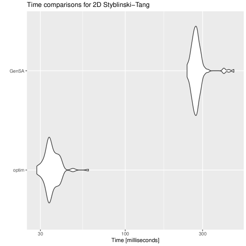
   Figure 2: Effect of constraints (each dimension constrained to be between $-5$ and $5$) viewed from the perspective of obtaining equivalent results on the Styblinski-Tang function in 2 dimensions

3.2.2 Object Oriented Designs

A C++ based class-oriented design has been described in the literature with UML diagrams [52], though it is not flexible enough to be extended easily to encompass the MCMC perspective. The basic components are to ensure data-abstraction and encapsulation of relevant information into objects, thus reducing the cognitive overload of the user when it comes to usage of the code-base. The package developed in subsequent sections is also object oriented, and its design is enumerated later.

4 Implementation

Recognizing that the SA algorithm is essentially driven by data, is a key abstraction. By tracking the history of the fitness functions, the temperature schedules may be altered, thus providing a further control knob for non-convex functions.

We base our design in two different directions, both implemented within the anneal package available on PyPI. Recognizing that most algorithmic approaches end up performing quenching instead of annealing, we implement both a quench interface which takes generic neighborhood construction, move classes, and acceptance criteria. However, additionally, as a novel addition, we will implement a Monte-Carlo Markov Chain class such that the time homogeneous chain can be simulated at each temperature. This frees the user from having to choose a set number of iterations at each temperature, instead continuing until the chains are mixed will using standard MCMC methods [48] as discussed earlier, assuming that the functions being minimized are integrable.

4.1 Class Hierarchy

We define a series of abstract classes that collectively form the API. In particular, as python does not have the same kind of semantics for virtual methods on classes, a slightly more verbose declaration is needed for each class using the Python standard library’s abc module. For the objective function, we expect it to have the following design as implemented in the eindir library:

⬇

class ObjectiveFunction(metaclass=abc.ABCMeta):

def __init__(self, limits: NumLimit, global_min: FPair = None):

self.calls = 0

self.limits = limits

self.globmin = global_min

@classmethod

def __subclasshook__(cls, subclass):

return (

hasattr(subclass, "__call__")

and callable(subclass.__call__)

and hasattr(subclass, "pointwise")

and callable(subclass.pointwise)

and hasattr(subclass, "multipoint")

and callable(subclass.multipoint)

and hasattr(subclass, "__repr__")

and callable(subclass.__repr__)

or NotImplemented

)

def __call__(self, pos):

if pos.ravel().shape[0] != self.limits.dims:

self.calls += 1

return self.multipoint(pos)

else:

self.calls += 1

return self.singlepoint(pos)

\par@abc.abstractmethod

def singlepoint(self, pos):

"""Evaluate the function at a single configuration"""

raise NotImplementedError(

"Need to be able to call the objective function on a single point"

)

\par@abc.abstractmethod

def multipoint(self, pos):

"""Evaluate the function at many configurations

"""

raise NotImplementedError

\par@abc.abstractmethod

def __repr__(self):

"""Name the function"""

raise NotImplementedError

In subsequent snippets, we will omit both the verbose __subclasshook__ check and basic double underscore (“dunder”) methods like __repr__ along with the comments. The entire code is implemented in the anneal library and is on GitHub along with a helper library for additional structures, both of which are under a permissive license (MIT) and are developed actively. We will also omit, for further brevity, the __init__ method, with the understanding that the initialization is straightforwardly a function of the arguments.

By construction, we have left open the option of having differing implementations (possibly with Python-C extensions) for evaluating a function on a single point and multiple points. We opt to use typing in cases where its usage makes the code-base more readable for end-users. In particular, we define a specialized class for handling constraints, and generating feasible points from a function’s range, that is, the limits data-class.

⬇

@dataclass

class NumLimit:

low: npt.NDArray

high: npt.NDArray

slack: float = 1e-6

dims: int = 1

def check(self, pos: npt.NDArray):

if not (

np.all(pos > self.low - self.slack)

and np.all(pos < self.high + self.slack)

):

raise OutOfBounds(

f"{pos} is not within {self.slack} of {self.low} and {self.high}"

)

return

\pardef mkpoint(self) -> npt.NDArray:

return np.random.default_rng().uniform(self.low, self.high)

\pardef clip(self, point: npt.NDArray) -> npt.NDArray:

return np.clip(point, self.low, self.high)

We also define, for ease of plotting and tracking data, a lightweight function evaluation structure:

⬇

@dataclass

class FPair:

pos: npt.NDArray

val: float

def EvalFunc(self, ObjFunc: callable):

self.val = ObjFunc(self.pos)

Which can be used to initialize a single point using python’s walrus operator for a given function F as x1 = FPair(pt := F.limits.mkpoint(), F(pt)). A list of such class structures can also be trivially converted to a pandas DataFrame for further analysis.

The heart of the implementation is twofold; a collection of abstract methods which are auxiliary to the traditional non-MCMC based SA, and an abstract class structure for working with MCMC samplers within an SA framework.

4.1.1 Quenching

Consider the heuristic approach:

⬇

class Quencher(metaclass=abc.ABCMeta):

def __init__(

self,

ObjFunc: ObjectiveFunction,

MkNeigh: ConstructNeighborhood,

Accepter: AcceptCriteria,

Mover: MoveClass,

Cooler: CoolingSchedule,

):

# OMITTED

pass

def __call__(self, trackPlot=False):

while (

temperature := self.Cooler(self.epoch)

) > 0.1 and self.epoch < self.maxiter.EPOCHS:

for step in range(1, self.maxiter.STEPS_PER_EPOCH + 1):

self.candidate = FPair(

pt := self.MkNeigh(self.cur.pos), self.ObjFunc(pt)

)

diff = self.DeltaFunc()

if diff <= 0:

self.AcceptMove()

else:

if self.Accepter(diff, temperature):

self.AcceptMove()

else:

self.RejectMove()

if self.HasConverged():

return

else:

self.epoch += 1

def DeltaFunc(self):

return self.candidate.val - self.cur.val

\pardef AcceptMove(self):

self.cur = self.candidate

if self.cur.val < self.best.val:

self.best = self.cur

else:

self.samestate_time += 1

self.acceptances += 1

\pardef RejectMove(self):

self.rejections += 1

self.samestate_time += 1

@abc.abstractmethod

def HasConverged(self):

raise NotImplementedError

Each of the objects passed in is essential to drive the algorithm but can be swapped out at will. Consider a concrete realization of the same, the standard Boltzmann simulated annealing, or BSA, which can now be implemented in a few lines.

⬇

class BoltzmannQuencher(Quencher):

def __init__(

self,

ObjFunc: ObjectiveFunction,

pos_init: npt.NDArray = None,

*,

T_init: float = None,

maxiter: MAX_LIMITS = MAX_LIMITS(int(1e6), int(1e3)),

):

self.ObjFunc = ObjFunc

self.Mover = BoltzmannMove(self.ObjFunc.limits)

self.MkNeigh = BoltzmannNeighbor(self.ObjFunc.limits, self.Mover)

self.Accepter = BoltzmannAccept()

self.T_init = T_init

self.Cooler = BoltzmannCooler(self.T_init)

super().__init__(

self.ObjFunc,

self.MkNeigh,

self.Accepter,

self.Mover,

self.Cooler,

)

self.epoch = 1

if pos_init is None:

self.cur = FPair(

pt := self.ObjFunc.limits.mkpoint(), self.ObjFunc(pt)

)

else:

self.cur = FPair(pt := pos_init, self.ObjFunc(pt))

self.maxiter = maxiter

## Initially

self.best = self.cur

While the input classes are straightforward implementations of the algorithm itself:

⬇

class BoltzmannCooler(CoolingSchedule):

def __init__(self, T_init, c_param=1):

self.c_param = c_param

super().__init__(T_init)

def __call__(self, epoch):

return (self.c_param * self.Tinit) / (1 + np.log(epoch))

class BoltzmannMove(MoveClass):

def __init__(self, limits: NumLimit):

self.limits = limits

def __call__(self):

return np.random.default_rng().normal()

class BoltzmannNeighbor(ConstructNeighborhood):

def __init__(self, limits: NumLimit, mover: BoltzmannMove):

self.limits = limits

self.stepper = mover

def __call__(self, c_pos):

candidate = self.limits.mkpoint()

proj = (

candidate * np.dot(c_pos, candidate) / np.dot(candidate, candidate)

)

dir_vec = proj / np.linalg.norm(proj)

final_cand = dir_vec * self.stepper()

return final_cand

class BoltzmannAccept(AcceptCriteria):

def __init__(self, k=1):

self.k = 1

def __call__(self, diff, Temperature):

metropolis = np.min([np.exp(-self.k * diff / Temperature), 1])

return np.random.default_rng().uniform(0, 1) < metropolis

Where most of the objects for this simple case are essentially almost equivalent to single function calls, but additional information and more complex structures can easily be incorporated. We also provide unified plotting and visualization tools for the derived classes of our hierarchy.

4.1.2 MCMC Approach

In keeping with our earlier discussion, the class-based approach yields more dividends here, as we are able to keep the same interface for the users, who will provide a function, and ensure that the class hierarchy will perform the necessary transformations.

⬇

class BaseChainSA(metaclass=abc.ABCMeta):

def __init__(

self,

ObjFunc: ObjectiveFunction,

Chain, # The type of chain used

Cooler: CoolingSchedule,

n_sim: int = 20000,

maxiter: MAX_LIMITS = MAX_LIMITS(int(1e6), int(1e3)),

):

self.ObjFunc = ObjFunc

self.n_sim = n_sim

self.stepNum = 0

self.epoch_best = []

self.Chain = Chain

self.epoch = 1

self.maxiter = maxiter

self.best = None

self.TargetDistrib = None

self.Cooler = Cooler

\pardef mk_target(self, Temperature):

return lambda point: np.exp(-self.ObjFunc(point) / Temperature)

\pardef __call__(self, Proposal, init_state=None):

if isinstance(init_state, type(None)):

init_state = self.ObjFunc.limits.mkpoint()

while (

temperature := self.Cooler(self.epoch)

) > 0.01 and self.epoch < self.maxiter.EPOCHS:

target = self.mk_target(temperature)

chain = self.Chain(target, Proposal, init_state)

for _ in range(self.n_sim):

chain.step()

self.epoch_best.append(self.getBest(chain.states))

if self.HasConverged():

return

else:

self.epoch += 1

\pardef getBest(self, statelist: list):

energies = np.array([self.ObjFunc(x) for x in statelist])

return FPair(pos=statelist[energies.argmin()], val=np.min(energies))

\pardef HasConverged(self):

min_ee = min([x.val for x in self.epoch_best])

self.best = [x for x in self.epoch_best if x.val == min_ee][0]

if min_ee == pytest.approx(self.ObjFunc.globmin.val, 1e-3):

self.fCalls = self.ObjFunc.calls

self.ObjFunc.calls = 0

return True

This can then be used to generate a simple MH sampler.

⬇

class MHChain:

def __init__(self, Target, Proposal, InitialState):

self.target = Target

self.proposal = Proposal

self.cstate = InitialState

self.states = []

\pardef step(self):

prop = self.proposal(self.cstate)

aproba = min(1, self.target(prop) / self.target(self.cstate))

if np.random.default_rng().uniform() < aproba:

self.cstate = prop

self.states.append(self.cstate)

\par\parclass MHChainSA(BaseChainSA):

def __init__(

self,

ObjFunc: ObjectiveFunction,

Cooler: CoolingSchedule,

n_sim: int = 5000,

maxiter: MAX_LIMITS = MAX_LIMITS(int(1e6), int(1e3)),

):

super().__init__(ObjFunc, MHChain, Cooler, n_sim, maxiter)

Whose API requires only a proposal distribution to be specified in addition to the standard requirements.

⬇

mhcsa = MHChainSA(ff, BoltzmannCooler(50))

mhcsa(np.random.default_rng().normal)

Where we have the flexibility to use any cooling schedule, and the base class can be extended to cover chain-tracking or the simulation of multiple chains at each temperature.

4.2 Representative Example

We will consider the Styblinski-Tang function in two dimensions as the candidate test function, visually depicted in Fig. 3 and defined as:

$$f(x^{*})=-39.16599d,\qquad x^{*}=(-2.903534,\ldots,-2.903534)$$

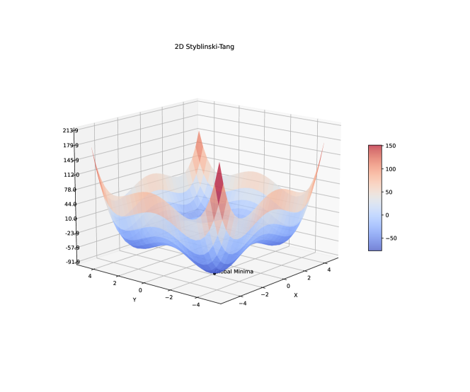
Figure 3: Styblinski-Tang function surface with the global minima indicated.

Implementation within the framework is achieved by:

⬇

import numpy as np

class StybTang2d(ObjectiveFunction):

def __init__(

self, limits=NumLimit(dims=2, low=np.ones(2) * -5, high=np.ones(2) * 5)

):

super().__init__(

limits,

FPair(val=-39.16599 * 2, pos=np.array([-2.903534, -2.903534])),

)

def singlepoint(self, pos):

self.limits.check(pos)

return np.sum((pos**4) - (16 * (pos**2)) + (5 * pos)) / 2

def multipoint(self, pos):

return np.apply_along_axis(

self.singlepoint, 1, pos.reshape(-1, self.limits.dims)

)

While results from its usage with a derived class are plotted in Fig. 4 and its usage is:

⬇

ff = StybTang2d()

# Quencher interface

bq = BoltzmannQuencher(StybTang2d(), T_init=5, pos_init=np.ones(2) * -2)

bq()

# Sampler interface

mhcsa = MHChainSA(ff, BoltzmannCooler(50))

mhcsa(np.random.default_rng().normal)

mhcsa.best

# Plotting

plttr = Plot2dObj(StybTangNd(2), 30)

plttr.plotQuenchContour(bq)

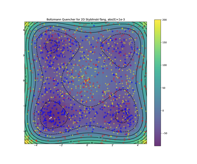
Figure 4: Styblinski-Tang 2D function surface with the Boltzmann Quencher. The yellow stars indicate points, which are accepted due to random acceptance, the red dots are rejected samples, and the blue dots are accepted samples.

5 Conclusions

We have demonstrated the design of a unified component-based system of working with simulated annealing which is capable of keeping pace with the current literature. This novel design incorporates not only the heuristic approaches but also the MCMC sampling-based alternative interpretation. Further exposition on numerical stability, the IEEE representation of numbers, heterogeneous computation, and data structures for functional data would be taking the discussion too far afield, though an expeditious next step would be the development of a domain-specific language, or DSL to encode further structure and algorithmically reduce the possibility of running inputs which have logical user errors. The design is flexible enough to be amenable to being parameterized by Neural Networks and other machine-learning approaches.

We have also had to necessarily restrict our design to that of a working applied scientist, and in doing so, have left out a discussion on the design of a formal software-based verification routine for this class of algorithms, along with symbolic implementations (e.g. with sympy) though the libraries discussed have these features planned.

The code alluded to is implemented in the anneal library , distributed on PyPI along with the eindir helper library .

Conflict of interest

The authors declare no conflict of interest.

References

- [1] Skúlason E, Bligaard T, Gudmundsdóttir S, Studt F, Rossmeisl J, Abild-Pedersen F, et al. A Theoretical Evaluation of Possible Transition Metal Electro- Catalysts for N 2 Reduction. Physical Chemistry Chemical Physics. 2012;14(3):1235-45.
- [2] Kumar P, Khan A, Goswami D. Importance of Molecular Heat Convection in Time Resolved Thermal Lens Study of Highly Absorbing Samples. Chemical Physics. 2014 Sep;441:5-10.
- [3] Prerna, Goswami R, Metya AK, Shevkunov SV, Singh JK. Study of Ice Nucleation on Silver Iodide Surface with Defects. Molecular Physics. 2019 Aug:1-13.
- [4] Karplus M, McCammon JA. Molecular Dynamics Simulations of Biomolecules. Nature Structural Biology. 2002 Sep;9(9):646-52.
- [5] Brunger AT. Simulated Annealing in Crystallography. Annual Review of Physical Chemistry. 1991;42(1):197-223.
- [6] Wille LT. Searching Potential Energy Surfaces by Simulated Annealing. Nature. 1986 Nov;324(6092):46-8.
- [7] Goswami D, Karnick H, Jain P, Maji HK. Towards Efficiently Solving Quantum Traveling Salesman Problem. arXiv:quant-ph/0411013. 2004 Nov.
- [8] Goswami D. Quantum Distributed Computing Applied to Grover’s Search Algorithm. In: Calude CS, Freivalds R, Kazuo I, editors. Computing with New Resources: Essays Dedicated to Jozef Gruska on the Occasion of His 80th Birthday. Lecture Notes in Computer Science. Cham: Springer International Publishing; 2014. p. 192-9.
- [9] Kirkpatrick S, Gelatt CD, Vecchi MP. Optimization by Simulated Annealing. Science. 1983 May;220(4598):671-80.
- [10] Metropolis N, Rosenbluth AW, Rosenbluth MN, Teller AH, Teller E. Equation of State Calculations by Fast Computing Machines. The Journal of Chemical Physics. 1953 Jun;21(6):1087-92.
- [11] Rutenbar RA. Simulated Annealing Algorithms: An Overview. IEEE Circuits and Devices Magazine. 1989 Jan;5(1):19-26.
- [12] Goswami R, Goswami A, Goswami D. Space Filling Curves: Heuristics For Semi Classical Lasing Computations. In: 2019 URSI Asia-Pacific Radio Science Conference (AP-RASC). New Delhi, India: IEEE; 2019. p. 1-4.
- [13] Russell SJ, Norvig P, Davis E. Artificial Intelligence: A Modern Approach. 3rd ed. Prentice Hall Series in Artificial Intelligence. Upper Saddle River: Prentice Hall; 2010.
- [14] Collins NE, Eglese RW, Golden BL. Simulated Annealing – An Annotated Bibliography. American Journal of Mathematical and Management Sciences. 1988 Feb;8(3-4):209-307.
- [15] Betancourt M. A Conceptual Introduction to Hamiltonian Monte Carlo. arXiv:170102434 [stat]. 2018 Jul.
- [16] Fox BL. Simulated Annealing: Folklore, Facts, and Directions. In: Niederreiter H, Shiue PJS, editors. Monte Carlo and Quasi-Monte Carlo Methods in Scientific Computing. Lecture Notes in Statistics. New York, NY: Springer; 1995. p. 17-48.
- [17] Salamon P, Sibani P, Frost R. Facts, Conjectures, and Improvements for Simulated Annealing. Society for Industrial and Applied Mathematics; 2002.
- [18] Ingber L. Simulated Annealing: Practice versus Theory. Mathematical and Computer Modelling. 1993 Dec;18(11):29-57.
- [19] Rouson D, Xia J, Xu X. Scientific Software Design: The Object-Oriented Way. New York: Cambridge University Press; 2011.
- [20] Goswami R. Wailord: Parsers and Reproducibility for Quantum Chemistry. Proceedings of the 21st Python in Science Conference. 2022:193-7.
- [21] Fox BL. Integrating and Accelerating Tabu Search, Simulated Annealing, and Genetic Algorithms. Annals of Operations Research. 1993 Jun;41(2):47-67.
- [22] A Stariolo D, Tsallis C. Optimization by Simulated Annealing: Recent Progress. In: Annual Reviews of Computational Physics II. vol. Volume 2 of Annual Reviews of Computational Physics. WORLD SCIENTIFIC; 1995. p. 343-56.
- [23] Lundy M, Mees A. Convergence of an Annealing Algorithm. Mathematical Programming. 1986 Jan;34(1):111-24.
- [24] Salazar R, Toral R. Simulated Annealing Using Hybrid Monte Carlo. Journal of Statistical Physics. 1997 Dec;89(5-6):1047-60.
- [25] Hansmann UHE. Simulated Annealing with Tsallis Weights a Numerical Comparison. Physica A: Statistical Mechanics and its Applications. 1997 Aug;242(1-2):250-7.
- [26] Press WH, editor. Numerical Recipes in C: The Art of Scientific Computing. 2nd ed. Cambridge ; New York: Cambridge University Press; 1992.
- [27] Mesirov JP. Accessible Reproducible Research. Science. 2010 Jan;327(5964):415-6.
- [28] Peng RD. Reproducible Research in Computational Science. Science. 2011 Dec;334(6060):1226-7.
- [29] Sandve GK, Nekrutenko A, Taylor J, Hovig E. Ten Simple Rules for Reproducible Computational Research. PLOS Computational Biology. 2013 Oct;9(10):e1003285.
- [30] Ioannidis JPA. What Have We (Not) Learnt from Millions of Scientific Papers with P Values? The American Statistician. 2019 Mar;73(sup1):20-5.
- [31] Dumiak M. Exascale Comes to Europe: Germany Will Host JUPITER, Europe’s Entry Into the Realm of Exascale Supercomputing. IEEE Spectrum. 2023 Jan;60(1):50-1.
- [32] Neal RM. MCMC Using Hamiltonian Dynamics. arXiv:12061901 [physics, stat]. 2012 Jun.
- [33] Yu VWz, Campos C, Dawson W, García A, Havu V, Hourahine B, et al. ELSI — An Open Infrastructure for Electronic Structure Solvers. Computer Physics Communications. 2020 Nov;256:107459.
- [34] Cohen J, Katz DS, Barker M, Chue Hong N, Haines R, Jay C. The Four Pillars of Research Software Engineering. IEEE Software. 2021 Jan;38(1):97-105.
- [35] Dolstra E, de Jonge M, Visser E. Nix: A Safe and Policy-Free System for Software Deployment. 2004:15.
- [36] Goswami R, Goswami A, Singh JK. D-SEAMS: Deferred Structural Elucidation Analysis for Molecular Simulations. Journal of Chemical Information and Modeling. 2020 Apr;60(4):2169-77.
- [37] Kedward LJ, Aradi B, Čertík O, Curcic M, Ehlert S, Engel P, et al. The State of Fortran. Computing in Science & Engineering. 2022 Mar;24(2):63-72.
- [38] Szu H, Hartley R. Fast Simulated Annealing. Physics Letters A. 1987 Jun;122(3):157-62.
- [39] Tsallis C, Stariolo DA. Generalized Simulated Annealing. Physica A: Statistical Mechanics and its Applications. 1996 Nov;233(1):395-406.
- [40] Fouskakis D, Draper D. Stochastic Optimization: A Review. International Statistical Review. 2002;70(3):315-49.
- [41] Bertsimas D, Tsitsiklis J. Simulated Annealing. Statistical Science. 1993 Feb;8(1).
- [42] Frenkel D, Smit B. Understanding Molecular Simulation: From Algorithms to Applications. Elsevier; 2001.
- [43] Ásgeirsson V, Jónsson H. Exploring Potential Energy Surfaces with Saddle Point Searches. In: Andreoni W, Yip S, editors. Handbook of Materials Modeling. Cham: Springer International Publishing; 2018. p. 1-26.
- [44] Wales DJ. Exploring Energy Landscapes. Annual Review of Physical Chemistry. 2018;69(1):401-25.
- [45] Chill ST, Welborn M, Terrell R, Zhang L, Berthet JC, Pedersen A, et al. EON: Software for Long Time Simulations of Atomic Scale Systems. Modelling and Simulation in Materials Science and Engineering. 2014 Jul;22(5):055002.
- [46] Xiang Y, Gubian S, Suomela B, Hoeng J. Generalized Simulated Annealing for Global Optimization: The GenSA Package. The R Journal. 2013;5(1):13.
- [47] Xiang Y, Sun DY, Fan W, Gong XG. Generalized Simulated Annealing Algorithm and Its Application to the Thomson Model. Physics Letters A. 1997 Aug;233(3):216-20.
- [48] Robert C, Casella G. Introducing Monte Carlo Methods with R. New York, NY: Springer New York; 2010.
- [49] Gelman A. Bayesian Data Analysis. Third edition ed. Chapman & Hall/CRC Texts in Statistical Science. Boca Raton: CRC Press; 2014.
- [50] Lyon GE. Using Ans Fortran. National Bureau of Standards; 1980.
- [51] Gamblin T, LeGendre M, Collette MR, Lee GL, Moody A, de Supinski BR, et al. The Spack Package Manager: Bringing Order to HPC Software Chaos. In: Proceedings of the International Conference for High Performance Computing, Networking, Storage and Analysis. SC ’15. New York, NY, USA: ACM; 2015. p. 40:1-40:12.
- [52] Ledesma S, Aviñ G, a, Sanchez R, Ledesma S, Aviñ G, et al. Practical Considerations for Simulated Annealing Implementation. In: Simulated Annealing. IntechOpen; 2008. .