A systematic search for short-period close white dwarf binary candidates based on the Gaia EDR3 catalog and the Zwicky Transient Facility data

Abstract

Galactic short-period close white dwarf binaries (CWDBs) are important objects for space-borne gravitational-wave (GW) detectors in the millihertz frequency bands. Due to the intrinsically low luminosity, only about 25 identified CWDBs are detectable by LISA, which are also known as verification binaries. The Gaia Early Data Release 3 (EDR3) provids a catalog containing a large number of CWDB candidates, which also includes parallax and photometry measurements. We cross-match the Gaia EDR3 and Zwicky Transient Facility public data release 8, and apply period-finding algorithms to obtain a sample of periodic variables. The phase-folded light curves are inspected, and finally we obtain a binary sample containing 429 CWDB candidates. We further classify the samples into eclipsing binaries (including 58 HW Vir-type binaries, 65 EA-type binaries, 56 EB-type binaries, 41 EW-type binaries) and ellipsoidal variations (209 ELL-type binaries). We discovered 4 ultra-short period binary candidates with unique light curve shapes. We estimate the GW amplitude of all our binary candidates, and calculate the corresponding signal-to-noise ratio for TianQin and LISA. We find 2 (6) potential GW candidates with signal-to-noise ratio greater than 5 in the nominal mission time of TianQin (LISA), which increases the total number of candidate verification binaries for TianQin (LISA) to 18 (31).

1 Introduction

Close White Dwarf Binaries are an important branch of the evolution channel of main-sequence star binaries (Gokhale et al., 2007). The formation of such binaries involves a stage of the common envelope, a complicated stage where complicated physical processes such as mass transfer, angular momentum loss, and even gravitational wave radiation. The theoretical simulation of the CWDBs evolution is challenging, with major issues still under debate. For example, it is not clear whether a second common envelope stage is involved in the formation of a CWDB. Since there are many sub-classes of CWDBs, there could be a variety of evolution channels. The searching and identification of new close white dwarf binaries have the potential to provide observational evidence for the binary evolution models and are important for the research of stellar physics, milli-Hertz gravitational-wave astronomy, and Galactic evolution.(Parsons et al., 2016; Rebassa-Mansergas et al., 2017; Lagos et al., 2020; Ren et al., 2020; Hernandez et al., 2021, 2022; Lagos et al., 2022).

Depending on the components type and mass transfer, CWDBs can be divided into several sub-populations (Ren et al., 2020; Inight et al., 2021; Kruckow et al., 2021): Post-Common Envelope Binaries, binary systems that contains a white dwarf and a main-sequence star; Cataclysmic Variables, interactive white dwarf binaries; and Double White Dwarfs.

Short-period CWDBs have orbital periods of less than 60 minutes, emitting gravitational wave (GW) in the millihertz-frequency band, becoming ideal sources for the space-borne gravitational wave observatories like the Laser Interferometer Space Antenna (LISA) (Amaro-Seoane et al., 2017) and TianQin (Luo et al., 2016; Gong et al., 2021), therefore, they are also known as verification binaries (VB)(Kupfer et al., 2018; Huang et al., 2020). The known classical verification binaries catalog includes 11 AM CVn-type binaries, 13 detached double white dwarfs, and 1 hot subdwarf binaries (Kupfer et al., 2018). Up to now, a total of $\sim$ 87 candidate verification binaries are all found in the electromagnetic band (Huang et al., 2020; Burdge et al., 2019a, 2020a, 2020b; Kilic et al., 2021; Chandra et al., 2021; Brown et al., 2022). In addition, there are other potential GW sources such as Helium star binaries, short-period CVs, exoplanets, brown dwarfs, and substellar companies (Amaro-Seoane et al., 2022). From the perspective of the formation pathways, these verification binaries and other potential GW sources experienced mass exchange phases via Roche-lobe overflow and mass loss via the ejection of a common envelope (CE) in evolution (Götberg et al., 2020; Amaro-Seoane et al., 2022). For example, there may be two different channels for the formation of DWDs: if the mass transfer stage is stable, it will be directly generated from CVs after a CE phase. If the mass transfer is unstable, the second CE stage takes place after the CVs, and then it will evolve into a WD+Helium-star, and finally form a DWD (Amaro-Seoane et al., 2022). It is noteworthy that El-Badry et al. (2021b) recently found evidence that the progenitors of extremely low mass white dwarfs (ELM WDs), AM CVn systems, and detached ultracompact binaries may be evolved CVs (El-Badry et al., 2021b, c). The Galactic foreground is mainly composed of DWDs, but other Galactic binaries also contribute to the Galactic foreground (Boileau et al., 2021), for example, CVs, stripped star binaries (Götberg et al., 2020), WD+M-dwarfs, etc.

In addition to searches from individual observations, one can perform CWDB search with a larger scale. Several surveys can be used to pick potential CWDB candidates, like the Catalina Real-time Transient Survey (CRTS) (Breedt et al., 2014), Global Astrometric Interferometer for Astrophysics (Gaia) (Geier et al., 2017; Gentile Fusillo et al., 2021; Rebassa-Mansergas et al., 2021; El-Badry et al., 2021a; Torres et al., 2022), the Optical Gravitational Lensing Experiment (OGLE) (Wevers et al., 2016), the Palomar Transient Factory (PTF) (van Roestel et al., 2017, 2018; Burdge et al., 2019b), the All Sky Automated Survey for SuperNovae (ASAS-SN) (Rivera Sandoval et al., 2022), the Transit Exoplanet Survey Satellite (TESS) (Wang et al., 2020; Pichardo Marcano et al., 2021a; Hernandez et al., 2022), the Large Sky Area Multi-Object Fiber Spectroscopic Telescope (LAMOST) (Wang et al., 2022b), and most recently the Zwicky Transient Facility (ZTF) (Ofek et al., 2020; Coughlin et al., 2020; Burdge et al., 2020a, b; Szkody et al., 2020, 2021; Kupfer et al., 2021; Keller et al., 2022; McWhirter & Lam, 2022). The repeated observations of the same sources can reveal the optical variability, and some of these surveys can be used, and have been used, to determine the periodicity.

In this paper, we present a search for CWDBs from a combination of survey data. We first select potential variable sources from the Gaia EDR3 catalog, then apply periodic analysis from time domain photometric data from ZTF data to determine the properties of the binaries.

The structure of this article is organized as follows. In Section 2, we elaborate the classification and the characteristics of the different sub-classes of close white dwarf binaries and the status quo of potential gravitational wave sources for these subtypes. In Section 3, we describe how to select our initial samples based on the Gaia H-R diagram, and further select the variable sample by the Gaia Variability Metric. In Section 4, we describe how we use three period-finding algorithms to search for periodic samples from ZTF light curves. In Section 5, we analyze five different variability types of binaries in our binary sample and compare our sample with the CWDBs catalog of other surveys. In Section 6, we discuss four interesting binaries. The overall parameter distribution and GW properties of the final sample are also discussed. Finally we summarize in Section 7.

2 Close White Dwarf Binaries and potential gravitational wave sources

There are two evolutionary pathways for primordial binaries: (1) The so-called wide binary, about 75% of wide binaries have relatively large orbital separations, and there is no interaction in the Hubble time-scale, which is similar to the evolution of a single star (Ren et al., 2020). (2) The remaining 25% are close binaries, which have to undergo a phase of mass transfer (Ren et al., 2020). After the ejection of the common-envelope (CE) phase, at least one star in the close binary evolved into a white dwarf, and due to complex physical processes such as angular momentum loss or gravitational wave radiation, which will be generated sub-classes such as PCEBs, CVs, and DWDs.

In this paper, we will focus on the Galactic ultra-compact white dwarf binary candidates that can generate gravitational wave radiation, potential gravitational wave sources, and the progenitors of GW sources. These targets are formed by the evolutionary pathway of the primordial binaries after the CE stage (Kruckow et al., 2021). We will focus on the classification and the characteristics of each sub-type of CWDBs: PCEBs, CVs, and DWDs, respectively.

2.1 Post-Common Envelope Binaries

PCEBs are detached or semi-detached binary systems in which a white dwarf and main-sequence star that is rapidly engulfed in a common envelope, and the orbital periods range from hours to a day. The companion stars in the PCEBs system are low-mass main-sequence stars, such as several brown dwarfs, M-dwarfs, hot subdwarfs, etc. Brown dwarf companion stars are difficult to search from optical band data alone, while M-dwarf and hot subdwarf companions are in the majority. Hot subdwarfs are under-luminous for their high temperature(Heber, 2016; Lei et al., 2020; Culpan et al., 2022). They are divided into two main spectroscopic: B-type subdwarfs (sdB, a core helium-burning star and thin hydrogen envelope), and O-type subdwarfs (sdO). Hot subdwarf binaries with white dwarf companions that exit the common envelope phase at orbital periods of less than two hours will overflow their Roche lobes while the sdB is still burning helium(Kramer et al., 2020; Li et al., 2022).

Striped star binaries are one of the populations of GW sources that can be detected by LISA (Götberg et al., 2020). Among them, the short-period hot subdwarf binaries are potential verification binaries for generating GW radiation. Until recently, only six known the ultra-compact sdB+WD-type binaries are VB sources with orbital periods less than 100 min, namely CD-30^∘11223 (Geier et al., 2013; Kupfer et al., 2018), HD 265435 (TIC 68495594, Pelisoli et al., 2021), ZTF J1946+3203, ZTF J0640+1738, ZTF J2130+4420, ZTF J2055+4651 (Burdge et al., 2020b; Kupfer et al., 2020a, b).

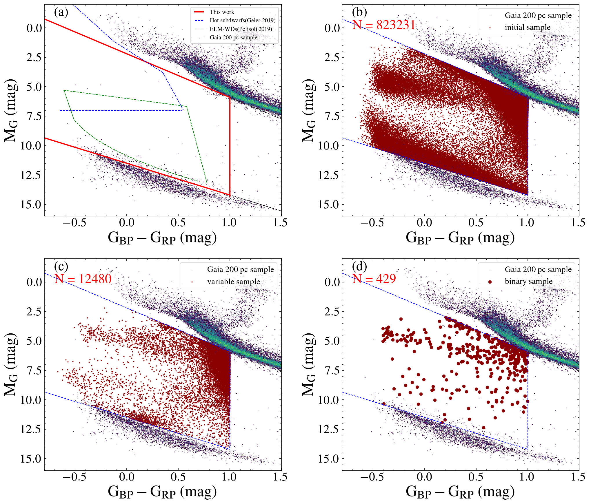
Figure 1: The location of the sample selection on the Gaia color-magnitude diagram. In all panels, scatter points and the overlaid 2D histogram shows the stellar density of the Gaia 200 pc background sources. (a) The red solid lines show the color-cut range that we defined, using the lower edge of the main sequence as an upper limit and the upper edge of the WD cooling sequence as a bottom limit, and using a color-cut $\rm G_{BP}-G_{RP}$ $<$ 1.0 as a right color limit. The blue dashed lines show a color-cut and absolute magnitude selection scheme for searching hot subdwarfs using Gaia data proposed by Geier et al. (2019). The green dashed lines show the color-magnitude diagram selection scheme for searching ELM-WD candidates based on Gaia DR2 data by Pelisoli & Vos (2019). (b) The red scatter points shows all samples under the initial query conditions. (c) The red scatter points shows the variable samples after using the Gaia variability metric select condition. (d) The red scatter points shows the final binary samples after examining ZTF light curve data.

2.2 Cataclysmic Variables

Cataclysmic variables are short-period ($\mathrm{P}_{\rm orb}\leq$ 6 h) semi-detached binary star systems in which a low-mass companion star transfers mass to a white dwarf (WD) primary via stable Roche lobe overflow(RLOF, Knigge et al., 2011; Hillman et al., 2020; Schreiber et al., 2021, 2022). The two stars are close enough that the companion completely fills its Roche lobe, and the outer layer of its envelope is gradually stripped from its surface and forms an accretion disk around the white dwarf. The CVs can be further divided into several sub-types: classical novae, dwarf novae, polar (AM Her-type star, Kolbin & Borisov, 2020; Kolbin et al., 2022), intermediate polar (DQ Her star, Norton et al., 1999) and AM Canum Venaticorum system(AM CVn, Nelemans et al., 2001a; Postnov & Yungelson, 2014; Ramsay et al., 2018; Wong & Bildsten, 2021), etc.

For the polar (B $\sim$10-200 MG) and intermediate polar (B $\sim$1-10 MG), the primary is a highly magnetized WD, and the accretion disk can be entirely disrupted. There are differences between polar and intermediate polars, the rotation of the white dwarf is synchronized with the orbital period of the companion in the polars, while the latter is not synchronized.

The AM CVn systems are short-period ultra-compact binaries in which a massive white dwarf accretes helium-rich matter from a hydrogen-deficient donor star. For AM CVn systems, the donors star are degenerate or semi-degenerate, and the orbital periods are in the range of $\simeq$ 5-68 minutes(Kalomeni et al., 2016; Green et al., 2018, 2020; van Roestel et al., 2021a, b; Duffy et al., 2021).

2.3 Double White Dwarfs

Double white dwarfs are the remnants of the second common envelope event in the evolution of close binaries. DWDs lose angular momentum through gravitational wave radiation, which will decrease the separation between the two white dwarfs and may eventually merge. Several relics can be associated with the double white dwarf merging event, such as type Ia supernovae (Nelemans et al., 2001b; Toonen et al., 2012; Shen et al., 2018; Liu et al., 2018; Rebassa-Mansergas et al., 2019; Maselli et al., 2020), neutron stars (Accretion-Induced Collapse events, Yu et al., 2019; Liu & Wang, 2020; Ablimit, 2022; Wang et al., 2022a) and high-mass WDs (Cheng et al., 2020). The exact outcome depends on the type of core of the two white dwarfs.

Extremely low-mass WDs are double-degenerate helium-core WDs with masses $M\leq 0.3M_{\odot}$. ELM WD systems are formed after severe mass loss, which limits that these systems most likely formed through binary interactions(Li et al., 2019). Because it is difficult to evolve into ELM WD from an isolated star in the Hubble timescale. The ELM survey is systematic search research for ELM WD binaries. This survey selects candidates by using SDSS color-cutting, then carried out the targeted spectroscopic follow-up of ELM WD candidates. The ELM survey successfully discovered 124 detached double-white dwarfs (DWDs)(Brown et al., 2010; Kilic et al., 2011; Brown et al., 2012; Kilic et al., 2012; Brown et al., 2013; Gianninas et al., 2015; Brown et al., 2016, 2020b; Kosakowski et al., 2020; Brown et al., 2022), including eleven systems which are strong candidate LISA-detectable gravitational-wave sources (Brown et al., 2011; Kilic et al., 2014; Brown et al., 2020a, 2022).

3 Target Selecion from Gaia EDR3

3.1 Gaia Color-Magnitude Diagram Selection

Gaia Early Data Release 3 (Gaia EDR3, Lindegren et al., 2021) contains more than 1.8 billion sources (the magnitude range from $\mathrm{G}=3-21$) with astrometric and photometric data based on the first 34 months of observations by the Gaia satellite. The astrometric data in the Gaia EDR3 provides positions, proper motions, and parallaxes ($\varpi$) for 1.468 billion sources, and the photometric data includes 1.544 billion sources which have magnitudes of photometric three-passbands G (phot_g_mean_mag), $\rm G_{BP}$, and $\rm G_{RP}$ (the BP and RP are defined by the blue and red photometers).

Thanks to the excellent astrometry measurement ability of Gaia, it can provide an accurate estimate of stars’ parallax. Compared with the Gaia DR2, the accuracy of parallax measurements of the Gaia EDR3 is improved by 20-30 percent on average. Meanwhile, the photometric observation ability enables the Gaia EDR3 to also provide color $\rm G_{BP}-G_{RP}$, and the G-band apparent magnitude of stars. Therefore, we can use the color-magnitude diagram to select our sample of object sources. Based on the distribution characteristics of known CWDB systems in the H-R diagram (Pelisoli & Vos, 2019; Inight et al., 2021), we find that the absolute magnitudes of these systems are dimmer than main sequence (MS) stars and brighter than single white dwarfs. We decide to apply the first cut in the color-magnitude diagram between the MS and white dwarf cooling sequence (WDCS). We further apply a selection condition on color $\rm G_{BP}-G_{RP}$ $<$ 1.0 to favor bluer objects, as white dwarfs are expected to have high temperatures. These first selection conditions are illustrated in Figure 1(a) as red solid lines. The corresponding equations are as follows:

$${\rm G_{BP}-G_{RP}}<1.0,$$ (1)

$${\rm G_{abs}<11.5+2.7\left(G_{BP}-G_{RP}\right)},$$ (2)

$${\rm G_{abs}>2.2+3.7\left(G_{BP}-G_{RP}\right)},$$ (3)

where $\rm G_{abs}=G+5*log10\left[(\varpi+0.029)/1000\right]+5$ is the absolute magnitude (Pelisoli & Vos, 2019). Our cutting scheme includes the selection range of extremely low-mass white dwarf candidates (green dashed lines in Figure 1(a)), and includes hot subdwarf stars (Geier et al., 2019) (blue dashed lines in Figure 1(a)).

To ensure that the red and blue photometry are not subject to random noise, we follow (Pelisoli et al., 2019; Pelisoli & Vos, 2019) and filtered on the errors of both $\rm G_{BP}$ and $\rm G_{RP}$ flux measurements to be larger than 10 (phot_bp/rp_mean_flux_over_error > 10). We also apply a signal-to-noise ratio (SNR) threshold of 5 on the parallax measurements (parallax_over_error > 5). The filter conditions for the threshold of parallax_over_error > 5 are often adopted for searches with Gaia data, for example, the search for ELM-WD candidates (Pelisoli & Vos, 2019), the search for pulsating white dwarfs (Guidry et al., 2021), the search for evolved-CVs (El-Badry et al., 2021b), and the search for AR Scorpii-type binary systems (Takata et al., 2022). Since the motivation of this work is to obtain reliable candidate GW sources, we conclude that precise measurement of parallaxes is very important so that the estimation of GW SNR can be trustworthy. By applying this filter, we exclude a large number of sources with positive and negative spurious parallaxes, especially near the color BP-RP $\sim 1$ in the Gaia H-R diagram.

Lindegren et al. (2018, 2021) proposed to apply the quality filter parameters selection condition on Gaia DR2, and Pelisoli (Pelisoli et al., 2019; Pelisoli & Vos, 2019) used similar conditions to the study of ELM-WD candidates. In this work, we apply the flux excess factor phot_bp_rp_excess_factor, $E$ as the quality filter parameters to the selection:

$$E<1.45+0.06\left(G_{BP}-G_{RP}\right)^{2},$$ (4)

$$E>1.0+0.015\left(G_{BP}-G_{RP}\right)^{2},$$ (5)

$$u<1.2\max(1,\exp(-0.2(G-19.5))),$$ (6)

where $\rm G$ is the G-band mean magnitude (phot_g_mean_mag), and u is defined by parameters the value of the chi-square statistic of the astrometric solution, astrometric_chi2_al, and the number of good observations, astrometric_n_good_obs_al:

$$u=\sqrt{\mathrm{astrometric\_chi2\_al/(astrometric\_n\_good\_obs\_al-5)}},$$ (7)

We plan to search for periodicity from the ZTF time-domain photometric data. However, the geographical site of ZTF put a limit on the archived data, so we apply a final cut in declination of $\delta>-28$ deg (Bellm et al., 2019; Graham et al., 2019; Masci et al., 2019; Dekany et al., 2020). For further details on the initial-cut selection criteria, please see Appendix A.

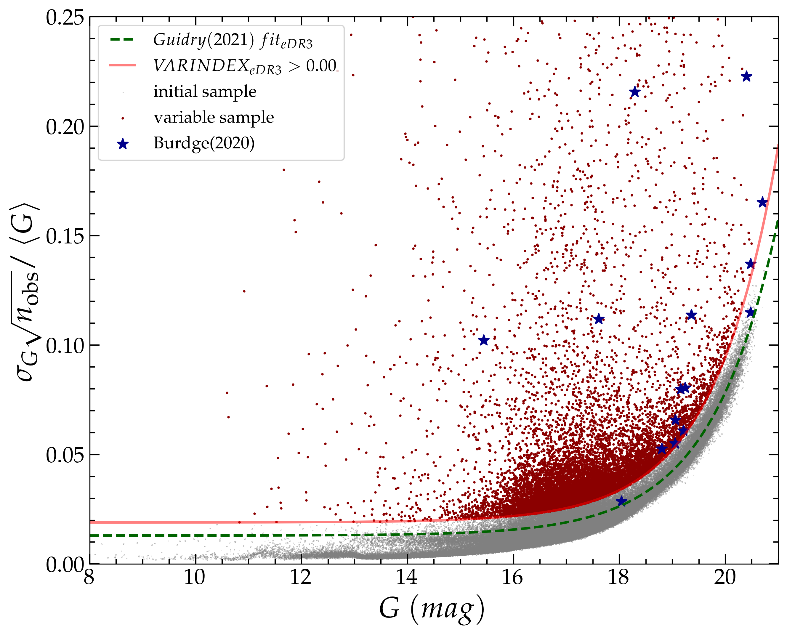
Figure 2: Empirical Gaia variability metric as a function of G-band magnitude for all initial samples, with the exponential fit proposed by Guidry et al. (2021) for Gaia EDR3 delineated in green. The 1.5 percent most variable samples are marked in red, and 15 ultra-compact binaries reported by Burdge et al. (2020a) are marked as blue stars.

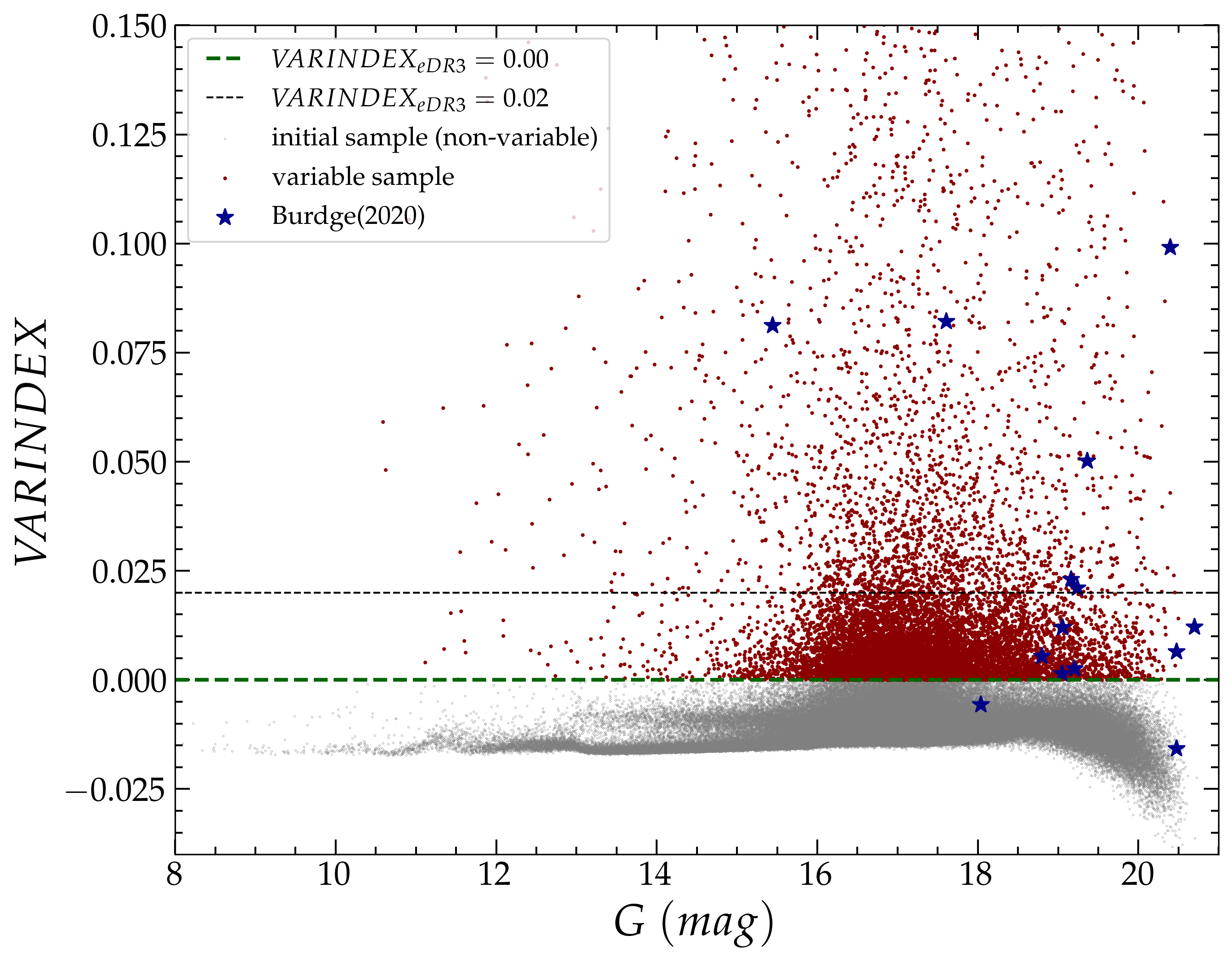
Figure 3: The VARINDEX and G band magnitude of the 12,480 candidates after Gaia variability cut. The green dashed line shows that 1.5 % of most variable samples have VARINDEX $>$ 0.00. The grey dashed line show El-Badry et al. (2021b) used VARIANDEX $>$ 0.02 to cut the samples in search of evolved-CVs. The 1.5 percent most variable samples are marked in red, and 15 ultra-compact binaries reported by Burdge et al. (2020a) are marked as blue stars.

3.2 Gaia Variability Metric

In the above section, in order to obtain clean initial samples, we have used a series of selection conditions, such as the the error of parallax measurements, and the quality of filtering parameter. Now our samples are accompanied with precise distance measurement and reliable photometric data. In this step, we aim to identify the variable sources that are most likely to be binaries. Therefore, we apply a further selection to the candidates from another dimension: photometric variability. The period search relies on the change of luminosity over time, and we can discard candidates with stable magnitudes, please see Appendix A. We apply a cut in the Gaia variability metric to select variable sources in the initial sample. We adopt the “variable amplitude” proposed by Deason et al. (2017) based on the root mean square (RMS) dispersion of flux. A number of studies have adopted the Gaia variable metric and successfuly identified different types of variable sources, including large-amplitude variables (Mowlavi et al., 2021), short-period cataclysmic variable (spCV) (Abrahams et al., 2020), pulsing white dwarf (Guidry et al., 2021), hot subdwarf stars (Barlow et al., 2022), and birth of the extremely low mass white dwarfs (El-Badry et al., 2021b, c). Following Guidry et al. (2021) and El-Badry et al. (2021b), we use the G-band photometris to further filter candidate with Gaia variability metric (or the variability amplitude proxy $\mathrm{A}_{\rm proxy,G}$, see Mowlavi et al. (2021)), $\rm V_{G}$:

$$V_{G}=\frac{\sigma_{G}}{\left\langle G\right\rangle}\sqrt{n_{{\rm obs}}},$$ (8)

where $n_{\rm obs}$ is the number of observations contributing to the G photometry (phot_g_n_obs), $\sigma_{G}$ is the error on G-band mean flux (phot_g_mean_flux_error ), $\left\langle\rm G\right\rangle$ is the G-band mean flux (phot_g_mean_flux). Figure 2 shows the Gaia variability metric distribution of the 823231 objects in the initial sample.

One can notice from Figure 2 that the Gaia variability metric is actually dependent on the G-band magnitude. This is because for dimmer objects, the associated SNR will be smaller, leading to a larger contribution from random fluctuation. In order to select the most-probable variable sources from the initial sample, we follow Guidry et al. (2021) and define the VARINDEX to cut the top 1% most variable CWDBs for Gaia EDR3:

$$\texttt{VARINDEX}=V_{G}-(Ae^{\alpha G}+Be^{G-17.0}+C),$$ (9)

where A = $8.31\times 10^{-9}$, $\alpha=0.794$, B = 0.0005, and C = 0.00962. In Figure 3, we show the distribution of the VARINDEX over G-band magnitude. We obtained the variable sample, which contains the 12480 strongest candidate variables with $\texttt{VARINDEX}>0.00$, as shown in Figure 1(c). It corresponds roughly to the 1.5% highest VARINDEX systems. We conclude that this choice is reasonable, since if we list the VARINDEX values of the 15 ultra-compact binaries reported by Burdge et al. (2020a), 13 of them are associated with $\texttt{VARINDEX}>0.00$, as shown in Figure 3. Even though 2 sources are discarded in this stage, this selection retains most of the interesting sources while greatly shrinking the sample size.

3.3 Variable Sample

We used the Gaia Variability flags to select 12480 candidates (see Table 1), which is defined as a variable sample of objects for period search. We imposed a photometric color selection of ${\rm G_{BP}-G_{RP}<1.0}$, this is different from the color-cut scheme used by Pelisoli & Vos (2019) to search for ELM candidates. Pelisoli & Vos (2019) used a color-cut criteron of ${\rm G_{abs}>20.25(G_{BP}-G_{RP})-7.15}$ to search for blue targets to reduce contamination sources such as faint red stars scattered from the main sequence. We are indeed interested in “blue” objects for the Gaia source catalog because we expected short-period CWDBs have higher temperatures due to tidal heating (Burdge et al., 2020b), especially those candidates whose orbital period is less than 60 min may become strong GW sources. However, we are also interested in other potential gravitational wave source candidates, such as short-period CVs and substellar companies (Amaro-Seoane et al., 2022). It is worth noting that our variable sample includes some outbursting objects, such as nonmagnetic CV (dwarf nova), magnetic CV (irregular variability on a wide range of timescales), and QSO (red-shifted emission lines) (Pelisoli & Vos, 2019), but these sources are considered as contamination in this study.

4 Zwicky Transient Facility Photometry

4.1 ZTF Light Curves

The ZTF is a time-domain survey using the 48-inch (P48) Schmidt telescope at Palomar Observatory. Its camera has a field of view of 47 square degrees, and it can scan the entire northern visible sky (Southern sky $\rm dec>-28$ deg.) at a rate of $\sim$ 3750 $\rm deg^{2}$ per hour (Bellm et al., 2019; Graham et al., 2019; Masci et al., 2019; Dekany et al., 2020). ZTF can reach a 5$\sigma$ limiting apparent magnitude of $\sim$ 20.8 mag in the $g$ band, $\sim$ 20.6 mag in the $r$ band, and $\sim$ 20.2 mag in the $i$ band in a 30s exposures.

For the selected variable sample, we cross match the coordinate with the ZTF data, by downloading light curve data from the ZTF Public Data Release 8 (ZTF DR8)^,.

4.2 Period Finding

The 12480 variable samples are not necessarily binary systems. To verify the binary nature of the system, the identification of the light curve period is necessary. To do so, we first cross-match the variable sample from Gaia data with the public ZTF 8th release data and identified 10938 sources that are accompanied by ZTF light curves. Then, we perform a period search procedure on the three time-series data: the ZTF-g band data, the ZTF-r band data, and the combined g + r band light curves.

Multiple algorithms can be used to the search of periodity from non-uniformly sampled data, including the Lomb-Scargle (LS) periodogram (Lomb, 1976; Scargle, 1982; VanderPlas, 2018), the Conditional Entropy (CE) algorithm (Graham et al., 2013a, b; Katz et al., 2021), and the Box Least Squares (BLS) algorithm (Kovács et al., 2002; Shahaf et al., 2022).

(i) The Lomb-Scargle periodogram is based on the Fourier transform and is used to detect and characterize the periodic component in unevenly sampled time-series data and generate a signal power spectrum (VanderPlas, 2018). The Lomb-Scargle normalized periodogram at frequency $f$ is defined as (Lomb, 1976; Scargle, 1982; Leroy, 2012).

$$P_{N}(f)= \frac{1}{2\sigma^{2}}\left[\frac{\left[\sum_{k}\left(y_{k}-\hat{y}\right)\cos\omega\left(t_{k}-\tau\right)\right]^{2}}{\sum_{k}\cos^{2}\omega\left(t_{k}-\tau\right)}\right.$$ (10)

$$\left.+\frac{\left[\sum_{k}\left(y_{k}-\hat{y}\right)\sin\omega\left(t_{k}-\tau\right)\right]^{2}}{\sum_{k}\sin^{2}\omega\left(t_{k}-\tau\right)}\right],$$

where $\omega=2\pi f$, $\sigma^{2}$ is the variance of the photometry, $y_{k}$ is the photometry at corresponding observation times $t_{k}(k=1,...,N)$, $\hat{y}$ is the mean of the photometry, and $\tau$ is the time-offset which is defined by Eq. (3) from Leroy (2012).

(ii) The Conditional Entropy algorithm is a period-finding method to find the period of an astronomical (irregularly sampled) time series data based on minimizing the conditional Shannon entropy when the light curve folded at the trial period (Graham et al., 2013a). The expression of the conditional entropy $H_{c}(m_{i}\mid\phi_{j})$ can be defined as (Graham et al., 2013a).

$$H_{c}\left(m_{i}\mid\phi_{j}\right)=\sum_{i,j}p(m_{i},\phi_{j})\ln\left(\frac{p(\phi_{j})}{p(m_{i},\phi_{j})}\right),$$ (11)

where $m$ is the normalized magnitude, $\phi$ is the phase (trial period), $p(m_{i},\phi_{j})$ is the density of points that fall within the bin located at phase $\phi_{j}$ and magnitude $m_{i}$, and p($\phi_{j}$) is the density of points that fall within the phi range. The CE algorithm determines the period through folding the phase of the light curve at each trial frequency, then estimating the conditional entropy of the partitioned phase-folded light curve corresponding to the trial frequency. In this paper, we used 10-magnitude bins and 20-phase bins in calculating the period of ZTF sources using the CE algorithm.

(iii) The Box-Least Squares algorithm is based on a simplified box-shaped model of a strictly periodic transit, which is characterized by using only five parameter estimators to find the best model (Kovács et al., 2002). The parameters used are the period ($P$), the transit duration as a fraction of the period ($q$), the phase offset of the transit ($\phi_{0}$), the difference between the out-of-transit brightness and the brightness during transit ($\delta$), and the out-of-transit brightness ($y_{0}$). The frequency spectrum of BLS can be defined by the amount of Signal Residue (SR) of the time series at any given trial period (Kovács et al., 2002):

$${\rm SR}=\max\left\{\left[\frac{s^{2}}{r(1-r)}\right]^{1/2}\right\},$$ (12)

where the equations of s and r are shown in Kovács et al. (2002), which can be used to estimate the photometric magnitude and the transit depth (Panahi & Zucker, 2021). The light curve of eclipsing binaries may generate the secondary eclipse, however, the secondary eclipse is in some cases too shallow to be detected. The BLS algorithm searches for the periodic dips in brightness for extrasolar planets, especially for the secondary eclipse.

The LS algorithm has the advantage of being very fast to execute, but the CE and the BLS algorithms can report a more accurate period and are more robust against noises. Therefore, we apply LS period search to all 10938 sources, but only apply CE and BLS analysis if the sources show reliable periodic features. The search strategy of the period is separated into two stages: the rough search and the fine search.

(1) In the first stage of the rough search for the period, the LS algorithm can quickly calculate each source with have good ZTF light curve data in the Variable sample, however, LS has a different sensitivity to objects with eclipsing binaries and sinusoidal sources, and LS is more sensitive to the latter, which results in that eclipsing binaries have twice the real period, and there exists a peak at half of the true frequency in the frequency spectra, as shown in Figure 5.

(2) In the second stage of the fine search for the period, we visually inspected the phase-folded lightcurves of 10938 sources and determined that 826 of them are promising periodic sources (see Table 1), which we define as the periodic sample. In this search, we adopt the cuvarbase implementation of the BLS and CE algorithms, please see Appendix C . A maximum frequency limit of 480 times per day is adopted. For the minimum frequency, we adopt the limit as twice the inverse of the baseline, where the baseline is defined as the end time minus the start time of the time-series data (for further details, please see Appendix B Period Finding Burdge et al. (2020b)).

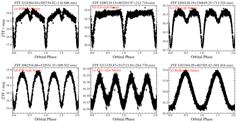
Figure 4: Examples of the variability types of light curve shapes caused by the binary eclipse effect in our binary sample. (a) HW Vir-type binary, in which a low-mass main-sequence star (M dwarf) orbits a core helium-burning sdO/sdB primary nearly edge-on (El-Badry et al., 2021b). (b) EA-type eclipsing binary, the unique shape of light curves is that between eclipses the light remains almost constant or varies insignificantly, and the light curves showing two minima per cycle or secondary minima may be absent. (c) EB-type eclipsing binary, showing two minima per cycle, and secondary minimum depth usually being considerably smaller than that of the primary minimum. (d) EW-type eclipsing binary, consisting of ellipsoidal components almost in contact, and the depths of the primary and secondary minima of the light curves are almost equal or differ insignificantly. (e) ELL-type binary, the light curve shape has the characteristics of quasi-sinusoidal variability produced by tidal deformation and shows two different minima in one orbit. (f) Reflection binary, in which an M dwarf orbits a hot white dwarf and is heated on one side (El-Badry et al., 2021b).

4.3 Periodic Sample

The classification criteria based on the Variable Stars Index catalog can be divided into two main variability groups: extrinsic variable stars and intrinsic variable stars. Extrinsic variable stars can be divided into eclipsing, rotating (spots, reflections, and ellipsoidal shapes), and microlensing events, of which the first two groups have obvious orbital modulation characteristics. The two main types of intrinsic variable stars are pulsation and outburst, in which pulsation is mainly the physical change inside the star. Based on the classification criteria of variable stars, we studied the general characteristics of the light curve shapes for binary systems and expected the physical mechanism of the variations.

Through multiple stages of search and veto, we are now left with a periodic sample of 826 candidates. More than $93.38\%$ of the variable sample are discarded, as they demonstrate irregular or non-variability and outburst characteristics, as shown in Figure 6. The physical origin of outbursting stars could be similar to the dwarf nova (CV) systems, especially the AM CVn-type systems (van Roestel et al., 2021c; Pichardo Marcano et al., 2021b). However, we have no reliable spectroscopic follow-up observations to confirm the binary nature of the systems. Therefore, we have to discard these sources for this study.

Figure 5: Examples of the variability types of light curve shapes caused by the binary eclipse effect in our binary sample. Panels (a1) to (f1) show the frequency spectra of the LS periodogram corresponding to the variability types of the phase folded ZTF light curve listed in Figure 4.

5 Analysis and Results

5.1 Binary Sample

According to the light curve shapes, the 826 candidates from the periodic sample can be further classified as eclipsing binary systems, such as the HW Vir-type eclipsing binary, the EA-type eclipsing binary (Detached Algol-type binaries), the EB-type eclipsing binary ($\beta$ Lyrae-type binaries) and EW-type eclipsing binary (W Ursae Majoris type binaries), ellipsoidal binary system (ELL-type lightcurve binaries), reflection system (Figure 4 (f) show the typical light curve shape of reflection binary: ZTF J183304.05+463705.42.), pulsation (the RR Lyrae type pulsating star and the delta Scuti type pulsating star), and rotation sinusoids, etc.

The final selection is to pick up sources demonstrating the obvious binary feature, like orbital modulation characteristics by binary motion, or showing light curves consistent with ellipsoidal or eclipsing models (see Table 1). Eventually, we produce a binary sample with 429 sources in total, as shown in Figure 1 (d). Among these, 220 are eclipsing binaries, and 209 are ellipsoidal binaries.

5.1.1 HW Vir-type Binaries

HW Virginis (HW Vir) systems are PCEBs composed of a sdO/sdB primary and a low-mass main-sequence star secondary (M-dwarf), e.g. sdB+dM systems for the prototype. HW Vir-type binaries mostly show variations in their orbital periods ($<$0.1 days), also called eclipse time variations (ETVs, Sale et al., 2020). The light curve of HW Vir systems shows that two distinct eclipses belong to the typical Algol-type eclipsing, but its light curve also has an out-of-eclipse variation, which is caused by the irradiation effect. Figure 4 (a) show the typical light curve shape of HW Vir-type binary: ZTF J234504.03+505754.82 (116.686 min). Among our eclipsing binary candidates, there are 58 HW Vir systems, accounting for 13.52$\%$ of all binary samples, as shown in Figure 7. We present the result of Gaia EDR3 data information of these candidates in Table 4, please see Appendix B.

5.1.2 EA-type Binaries

EA-type eclipsing binaries are also called detached Algol-type binaries. Based on the definition of the Variable Stars Index Catalog, the unique shape of light curves are that between eclipses the light curve remains almost constant or varies insignificantly. The explanation for this characteristic is that binaries have spherical or slightly ellipsoidal components, and the reflection effects or physical variations are also important factors.

Detached white dwarf binaries, can have different effective temperatures and can show eclipse variability in the photometric data. If the binary has a high inclination angle, then the phase-folded light curve will contain two eclipses, a deeper primary one and a shallower secondary one. The primary eclipse is generated when the brighter target is obscured by its companion, and the secondary eclipse is the opposite process. In some cases, however, the secondary eclipse is too shallow to be detected, and there is only a primary eclipse in one orbit. Out of 220 eclipsing binary candidates in the binary sample, 167 sources illustrate both primary and secondary eclipses, and only primary eclipses are identified for the remaining 59 sources. Figure 4 (b) show the typical light curve shape of EA-type eclipsing binary: ZTF J200119.16+482301.88 (212.716 min). Among our eclipsing binary candidates, there are 68 EA-type eclipsing binaries, accounting for 15.15$\%$ of all binary samples, as shown in Figure 7. We present the result of Gaia EDR3 data information of these candidates in Table 5 in Appendix B.

Figure 6: The pie chart of the percentage of binaries for particular variability classes in our variable sample.

5.1.3 EB-type Binaries

EB-type ($\beta$ Lyrae-type) eclipsing binary systems have ellipsoidal components and light curves for which it is impossible to specify the exact times of onset and end of eclipses because of a continuous change of the system’s apparent combined brightness between eclipses. The secondary minimum is observed in all cases, its depth usually being considerably smaller than that of the primary minimum. Figure 4 (c) show the typical light curve shape of EB-type eclipsing binary: ZTF J204328.19+230649.25 (712.524 min). Among our eclipsing binary candidates, there are 56 EB-type eclipsing binaries, accounting for 13.05$\%$ of all binary samples, as shown in Figure 7. We present the result of Gaia EDR3 data information of these candidates in Table 6 in Appendix B.

Table 1: Summary of the numbers of close white dwarf binary candidates at different stages and different types.

Sample	Type	Identified Sources	Unidentified Sources	Number
$\mathbf{Selection~{}on~{}Gaia~{}data}$
Initial sample	$...$	$...$	$...$	823231
Variable sample	$...$	$...$	$...$	12480
$\mathbf{Selection~{}on~{}ZTF~{}data}$
Periodic sample	$...$	$...$	$...$	826
	HW Vir-type (Algol-type) binaries	6	52	58
	EA-type (Detached Algol-type) binaries	14	51	65
Binary sample	EB-type ($\beta$ Lyrae-type) binaries	3	59	56
	EW-type (W Ursae Majoris-type) binaries	1	40	41
	ELL-type (Ellipsoidal) binaries	20	183	209
	$\mathbf{Subtotal}$	$\mathbf{44}$	$\mathbf{385}$	$\mathbf{429}$

Note. — It is worth noting that we have statistics on the sources that have been confirmed by spectroscopic follow-up observations or spectral energy distribution analysis, which as Identified Sources.

5.1.4 EW-type Binaries

EW-type eclipsing binaries are also known as W Ursae Majoris type binaries, which are composed of ellipsoidal components almost in contact, and eclipses in binary systems with components filling their Roche-lobes. The depths of the primary and secondary minima of the light curves are almost equal or differ insignificantly. The amplitude variations of light are usually less than 0.8 mag and the orbital periods are usually shorter than one day. Figure 4 (d) show the typical light curve shape of EW-type eclipsing binary: ZTF J082516.60+432931.35 (309.922 min). Among our EW-type eclipsing binary candidates, there are 41 EW-type eclipsing binaries, accounting for 9.56$\%$ of all binary samples, as shown in Figure 7. We present the result of Gaia EDR3 data information of these candidates in Table 7, please see Appendix B.

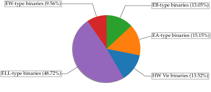
Figure 7: The pie chart of the percentage of binaries with the different types of light curve shapes in our binary sample.

5.1.5 ELL-type Binaries

ELL-type binaries (ellipsoidal variables) are non-eclipsing reflection effect binaries consisting of a hot white dwarf and a cooler companion (typically an M dwarf) (El-Badry et al., 2021b). The variability amplitudes are usually less than 100 mmag. In the ellipsoidal modulation system, the shape of the light curve has the characteristics of quasi-sinusoidal variability and shows two different minima in one orbit. This quasi-sinusoidal variation light curve is produced by tidal deformation, in which case the two sides of the tidally disturbed star have different temperatures, and the hotter side is brighter than the colder side. There are two different minima in the light curve, which is mainly caused by the gravity darkening effect. Figure 4 (e) show the typical light curve shape of ELL-type eclipsing binary: ZTF J213329.86+512721.88 (264.770 min). We identify 209 candidates to be ellipsoidal variables, which account for 48.72$\%$ of the binary sample, as shown in Figure 7. We present the result of Gaia EDR3 data information of these candidates in Table 8 in Appendix B.

5.2 Comparison to the other catalogs

Our screening scheme provides a candidate catalog covering different types of close white dwarf binaries, which provides observational evidence for the study of the evolutionary channels of white dwarf binaries.

Several studies feature the search of CWDB systems. We compare our samples and cross-check the identified binaries with these works.

Burdge et al. (2020a, b) used the Pan-STARRS1 catalog and ZTF photometric data to search for potential sources for milli-Hz band gravitational wave detectors. They successfully discovered sixteen ultra-compact binaries, including eight eclipsing systems, two AM CVn systems, and six ellipsoidal variations systems. Two of the sources, namely ZTF J213056.69+442046.58 (orbital period 39.340 min) and ZTF J205515.96+465106.45 (orbital period 56.348 min), are also identified in our search. Both sources are mass-transferring WD+sdB systems, and their light curves have similar shapes, which are typical ellipsoidal variables (see Kupfer et al. (2019, 2020a, 2020b, 2022) for further details). We analyzed the reason why only two sources in our sample overlap with the 15 ultra-compact binaries reported by Burdge et al. (2020a). We checked the Gaia astrometric parameters of these 15 ultra-compact binaries and found that only three sources are measured with parallax_over_error $>$ 5, which means that most sources are filtered out by our initial selection criteria for lack of reliable distance estimation, see Section 3.1 for further details.

El-Badry et al. (2021b) selected sources in the Gaia color-magnitude diagram and searched for large-amplitude ellipsoidal variability using ZTF photometric data. Their motivation is to find the progenitor of extremely low-mass white dwarfs and AM CVn systems. In El-Badry et al. (2021b), the authors reported 51 candidates, of which 21 sources obtained many-epoch spectra, and all 21 sources were confirmed to be completely or nearly Roche lobe filling binaries, 13 showing evidence of ongoing mass transfer. Our 22 ellipsoidal variable candidates reported by El-Badry et al. (2021b), and 11 sources have been confirmed by spectra. The initial query conditions we used for sample selection in Gaia EDR3 are different from El-Badry et al. (2021b).

Keller et al. (2022) used the published catalog compiled by Gentile Fusillo et al. (2019) to identify eclipsing white dwarf binaries. They used the BLS algorithm to search for sources with periodic light curve variability in the ZTF data, and their search revealed 18 new binaries. The cross-check between our binary sample and these 18 binaries reveals five binaries to be overlapped. Keller et al. (2022) used samples from the Gaia white dwarf catalog, which contains 486641 sources. They cross-matched Gaia white dwarf catalog with ZTF DR3 data and finally obtained 276074 sources that have at least two ZTF epochs. We used the variable sample which was selected after the Gaia Variability Metric cut to cross-match the ZTF DR8 data. This leads to the discard of a large fraction of faint sources and could explain the difference in reported samples.

Wang et al. (2021) systematically searched for periodic variables in the hot subdwarf catalog from Gaia DR2 using ZTF data. Their targets come from a catalog of 39,000 hot subdwarf candidates provided by Geier et al. (2019). In their search, they found 67 HW Vir binaries and 496 sources with reflection effects or pulsation, plus a few eclipsing and ellipsoidally modulating binaries. Our selection criteria in Gaia color-magnitude diagram include the hot subdwarf region in Section 3.2 of Geier et al. (2019). Therefore, our candidates will inevitably overlap with Wang et al. (2021). However, the catalog is not publicly available, therefore we can not check the extent of overlap.

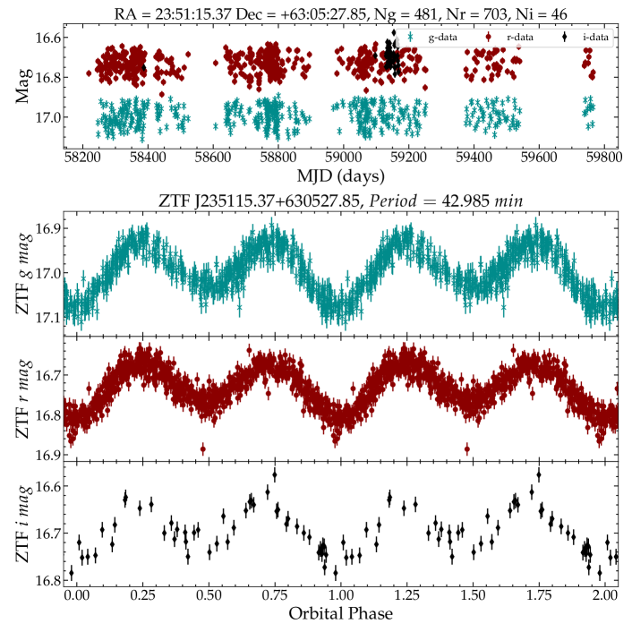
Figure 8: The light curves of ZTF J235115.32+630528.23. The top panel shows the raw ZTF g (dark cyan), r (dark red), and i (black) light curves. The middle and the bottom panel show the ZTF g-band and r-band folded light curves, respectively. Archival ZTF g-band and r-band light curves of the system folded at a period of 42.985 minutes.

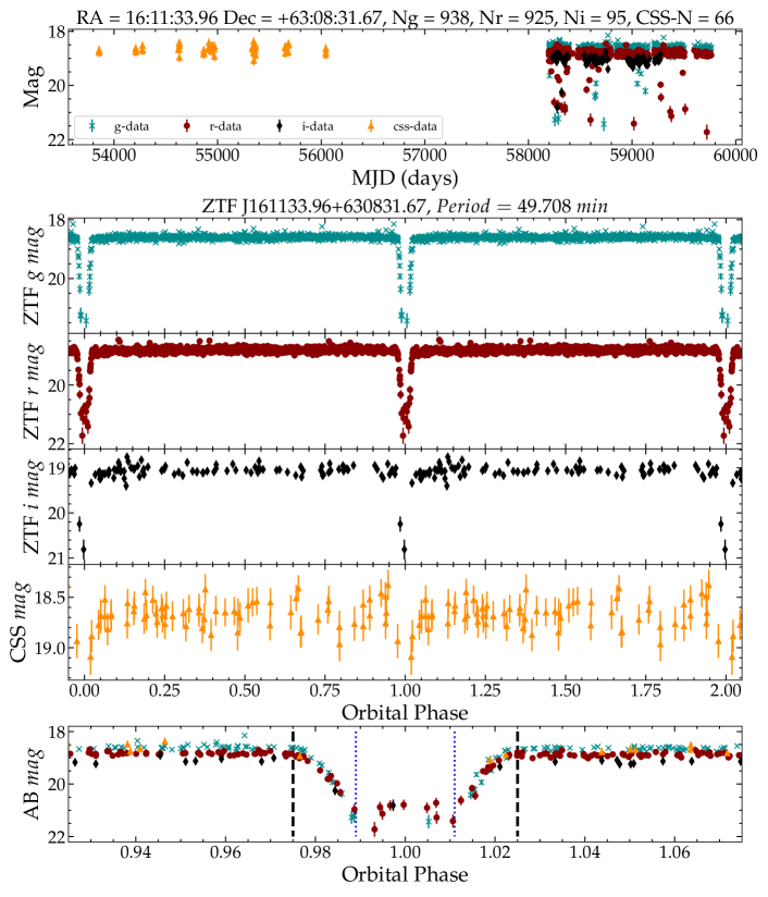
Figure 9: The light curves of ZTF J161133.96+630831.67. The top panel shows the raw ZTF g-band (dark cyan), r-band (dark red), and i-band (black) light curves, and raw CSS (dark orange) photometric data. The middle panels show the phased ZTF light curves for the g-band, r-band, and i-band, and the phased CSS light curve, respectively. The bottom panel shows the phase-folded light curves of ZTF J1611+6308 at phase $\phi\sim$ 0.975-1.025 in the eclipse duration. The blue dashed lines show the duration of the conjunction of the eclipse, and the black dashed lines show the entire duration of the eclipse from ingress to egress. Archival ZTF (g-, r-, and i-band), and CSS light curves of the system folded at a period of 49.708 minutes.

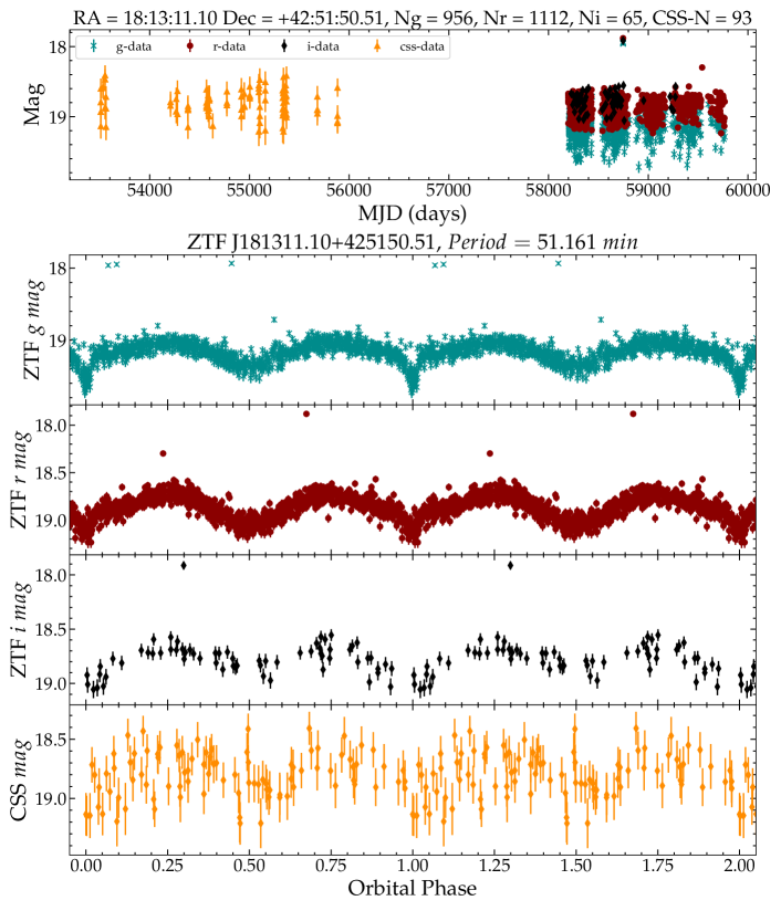
Figure 10: The light curves of ZTF J181311.10+425150.51. The top panel shows the raw ZTF g-band (dark cyan), r-band (dark red), and i-band (black) light curves, and raw CSS (dark orange) light curves. The middle and the bottom panels show the phased ZTF (g-band, r-band, and i-band), and phased CSS light curves for ZTF J1813+4251, respectively. Archival ZTF (g, r, and i), and CSS light curves of the system folded at a period of 51.161 minutes.

Figure 11: The light curves of ZTF J011242.48+582757.60. The top panel shows the raw ZTF g-band (dark cyan) and r-band (dark red) light curves. The middle and bottom panels show the phase-folded light curves for ZTF J0112+5827 in g and r-bands, which show a clear difference between the two bands. The r-band exhibit two obvious spikes in one phase, between two spikes there is a transit phase.

6 Discussion

6.1 Notes on Individual Objects

We selected four sources with special light curve shapes from the candidates, which are ZTF J2351+6305, ZTF J1611+6308, ZTF J1813+4251, and ZTF J0112+5827. The four newly discovered CWDB candidates have distinct light curve variability. Three sources are accompanied by an orbital period of less than 60 minutes and that of the other source is about 81 minutes. To understand the composition of these candidates and to explain the feature of the light curves, we will apply a large aperture telescope for time-domain photometry and spectral follow-up observations.

ZTF J235115.32+630528.23 (ZTF J2351+6305) is an ultra-short period binary candidate. Its phase-folded light curve shows ellipsoidal variation characteristics (as shown in Figure 8), and the BLS period is 42.985 minutes. It has a color of $G_{\rm BP}-G_{\rm RP}=0.59$ mag and a magnitude of $G_{\rm abs}=6.24$ mag. It may be a mass-transferring and recently-detached CV, which is a progenitor of ELM-WDs or AM CVn systems. El-Badry et al. (2021b) has systematically studied such systems. Among their 51 candidates of evolved CVs and bloated proto-ELM WDs, the shortest orbital period is 2 hours. This candidate has a shorter orbital period than reported by El-Badry et al. (2021b). The donor of evolved CVs has high temperatures ($4700<T_{\rm eff}<7000\rm K$), which can be confirmed by spectral follow-up observation.

ZTF J161133.96+630831.67 (ZTF J1611+6308) has a period of 49.708 min. The ZTF phase-folded light curve shows a deeply-eclipsing white dwarf binary characteristic and the eclipse depth is greater than 2.5 mag, as shown in Figure 9. ZTF J1611+6308 has a color of $G_{\rm BP}-G_{\rm RP}=0.19$ mag and magnitude of $G_{\rm abs}=11.26$ mag. The Catalina Sky Survey observed ZTF J1611+6308 between 2005 and 2013, and we obtained clean raw photometric data of CSS for ZTF J1611+6308. Figure 9 shows the phased ZTF light curves for the g-band, r-band, and i-band, and the phased CSS light curve. The light curve has a deep eclipse, but there is no secondary eclipse, and the eclipse duration is about 2.5 minutes as shown in the bottom panel of Figure 9. We used twice the period to fold the light curve, and the primary and secondary eclipses appeared at the same depth. The evolution of the light curve is predicted to be dominated by a white dwarf, while the companion star is a low luminosity target, such as a brown dwarf or an M dwarf (Kosakowski et al., 2022). The classification of the system can be further confirmed by spectrum and high-speed photometric observation.

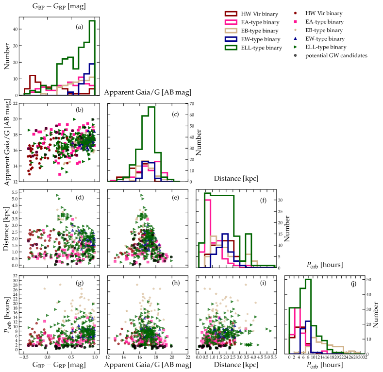
Figure 12: The corner plot for the main parameters of different types of light curve shapes of binaries within our binary sample. In panel (a), (c), (f), and (j), we show the one-dimensional histogram over Gaia BP-RP color, the Gaia G-band apparent magnitude, the distance, and the orbital period, respectively. Other panels (b, d, e, g, h, i) show the correlation distribution between the two parameters for different types of binaries.

ZTF J181311.10+425150.51 (ZTF J1813+4251) is a cataclysmic variable candidate with a period of 51.161 min.

The light curve is a fully eclipsing binary system characteristic that is similar to the ZTF J1946+3203 (Burdge et al., 2020b), which exhibits strong ellipsoidal variations owing to the tidal deformation and eclipse effect as shown in Figure 10. ZTF J1946+3203 is a single-lined spectroscopic eclipsing binary, which is composed of a hot He WD or an sdB and a low luminosity He WD companion star. In the color-magnitude diagram, ZTF J1813+4251 is located in the classical CV region at $G_{\rm BP}-G_{\rm RP}=0.79$ mag, and an absolute magnitude of $G_{\rm abs}=9.36$ mag, which is significantly different from the position of ZTF J1946+3203. We obtained clean raw photometric data of CSS and ZTF for ZTF J1813+4251, as shown in the upper panel of Figure 10. Further observations of ZTF J1813+4251 are needed to measure the radial velocity and to strongly constrain the masses, radii, and temperatures using high-speed photometry. Once confirmed, this may be the shortest orbital period CV system ever observed. During the preparation of this manuscript, Burdge et al. (2022) reported the observation of this source. They found that ZTF J1813+4251 is a transitional CV, and this binary consists of a star with a temperature comparable to that of the Sun but a density 100 times greater owing to its helium-rich composition, accreting onto a white dwarf. These transitional CVs have been proposed as progenitors of helium CVs (Burdge et al., 2022).

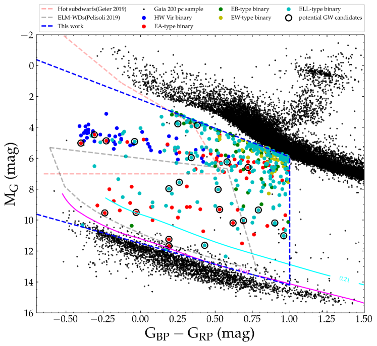
Figure 13: The location of the binary samples on the Gaia H-R diagram. The blue dashed lines show our selection scheme for searching CWDBs based on Gaia EDR3 data. The red dashed lines show that the selection rule proposed by Geier et al. (2019) based on Gaia DR2 data to search the population of hot subdwarfs. The black dashed lines show that the selection scheme proposed by Pelisoli & Vos (2019) based on Gaia DR2 data to search ELM-WD candidates. The solid red line is the cooling model offset by $-0.75$ mag for 0.21$M_{\odot}$ and 0.69$M_{\odot}$ white dwarf. We use the publicly available WD_models package provided by Cheng et al. (2020). The black scatter points show the Gaia 200 pc background sources. The five colors scatter points show the different types of light curve shapes in the final binary samples searched using ZTF data, and the black circles show the binaries in the Binary sample whose period is less than 100 min, which are potential GW source candidates.

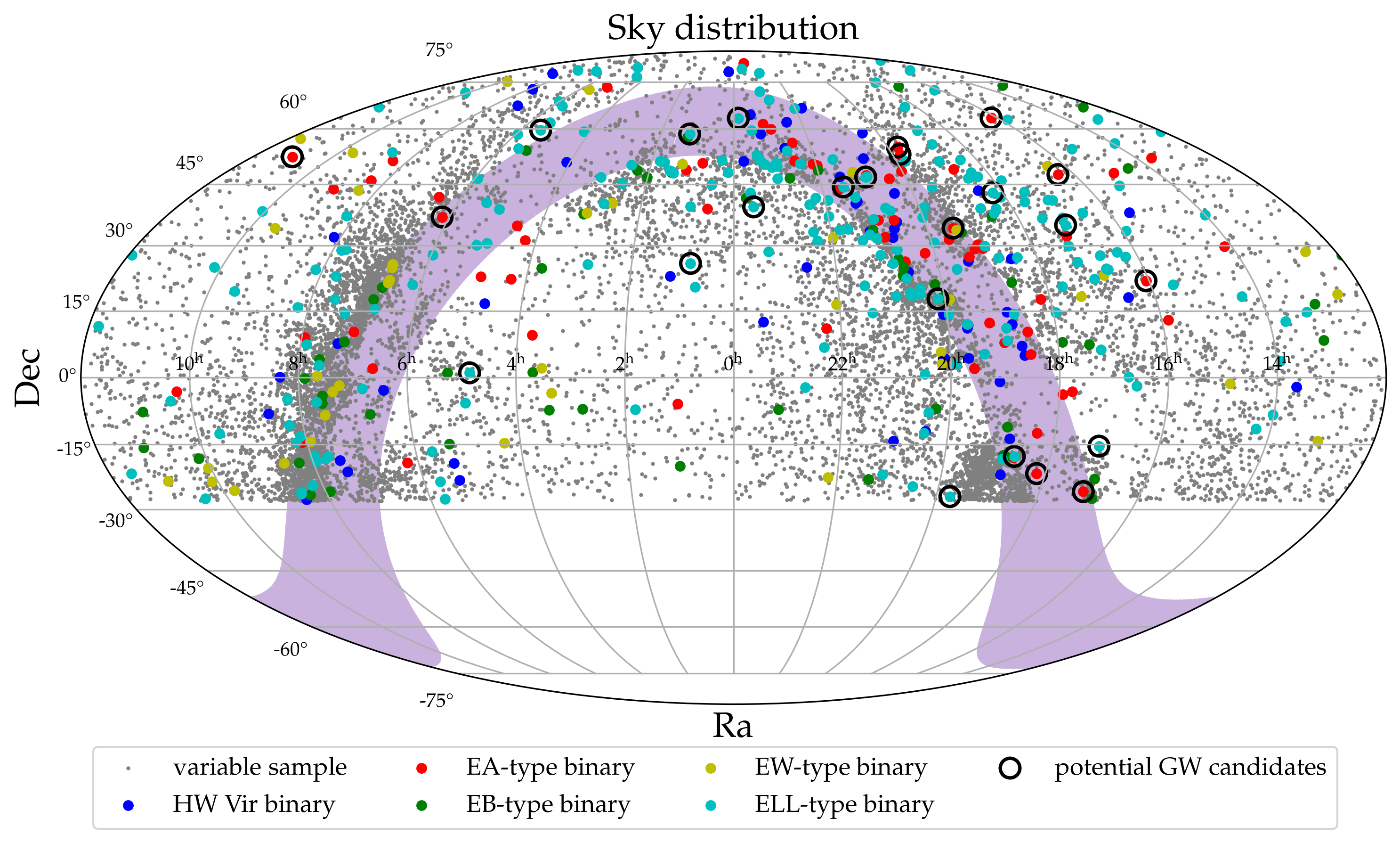
Figure 14: Sky distribution in equatorial coordinates of the variable sample (gray dots) and the Binary sample (color dots). The black circles show the potential GW source candidates.

ZTF J011242.48+582757.60 (ZTF J0112+5827) is a CV candidate, which has a color of $G_{\rm BP}-G_{\rm RP}=0.9$ mag and magnitude of $G_{\rm abs}=10.19$ mag. The light curve of ZTF J0112+5827 shows typical large-amplitude ellipsoidal variation in the g-band, and the period computed by the BLS algorithm is 80.9 minutes, however, its r-band light curve shows an unusual two spikes in one period, as shown in Figure 11. We propose a possible hypothesis to explain the unusual light curve of ZTF J0112+5827: This is a polar (AM Her-type star) or intermediate polar. The accreted mass moves along the magnetic lines in the direction of the white dwarf’s magnetic poles. The two spikes of the light curve in one period are generated by the accretion point, which is similar to a rare eclipsing polar BS Tri system (Kolbin et al., 2022). Future high-time resolution spectral observations will be needed to verify the formation of the unusual light curve of the binary system.

6.2 Parameters Distribution of CWDBs

In order to better understand the distribution characteristics of photometric parameters and source parameters of different types of candidates in our binary sample, we display their statistical histograms and correlations in Figure 12.

Figure 12 (a) shows the Gaia BP-RP color index distribution for different types of binaries. HW Vir binaries are mainly distributed at BP-RP $<$ 0 mag, because hot subdwarfs have a high surface temperature and they appear to be bluer. Other variability types of binaries are mainly distributed at BP-RP $>$ 0 mag, where ELL-type binaries are generally distributed between 0.2 mag $<$ BP-RP $<$ 1.0 mag. Figure 12 (c) shows the apparent magnitude distribution of Gaia/G-band of different types of candidates, which scatters between 16-18 mag. In Figure 12 (f), we show the distance distribution of all binary candidates, HW Vir binary and EW-type binaries are mainly between 1.0 kpc to 2.5 kpc, EA-type binary at 0.5-2.0 kpc, the EB-type binary at 1.0-2.0kpc. Figure 12 (j) shows the orbital period distribution of these binary candidates. We find that for most types of binaries, the orbital periods are mostly less than 9 hours, while EB-type binary exhibits a peak at around 10 hours. We can explain the period distribution by the fact that the viewing angle will be decreasingly small for wider seperated eclipsing binaries. The ELL-type does not subject to this selection bias as they do not rely on eclipsing observation. The HW-type are also not affected as the component size are usually larger, corresponding to a larger viewing angle.

Other panels (b, d, e, g, h, i) in Figure 12 show two dimensional distribution for different types of binary systems. For example, from Figure 12 (d) and (e), we find an apparent cut in the upper right corner. This is most likely due to the choice of the Gaia variability metric.

6.3 The Gold Sample of CWDBs

In the H-R diagram, the sub-types of CWDB are mostly located in the region between MS and WDCS. We divided the volume according to the types of close binary stars in the H-R diagram and defined three gold samples, namely PCEBs gold sample, CVs gold sample, and DWDs gold sample. Inight et al. (2021) established a volume-limited sample for all sub-types of CWDB, which can be used to study the population of WD binaries. The reference samples provide four types of gold samples: WD + M (M-type main-sequence star), WD + AFGK (A, F, G, or K-type star), CV, and DWD. Our gold samples are not established by spectral type. We define the gold samples based on Gaia selection source conditions proposed by Geier et al. (2019) and Pelisoli & Vos (2019) and combined them with the white dwarf cooling model. We show the distribution characteristics of these binary candidates in the H-R diagram in Figure 13, and their sky distribution in Figure 14.

Geier et al. (2019) applied a color-cut and absolute magnitude selection to define a distribution range of hot subdwarf candidates in Gaia DR2, as shown in Figure 13 (the red dashed lines). We further define the sdB binaries (or PCEBs) in this region as the gold sample (see Table 2). We have a total of 85 hot subdwarf binary candidates as gold samples, of which 6 have orbital periods less than 100 min.

Table 2: Summary of the differences in the number of the gold sample

Object Type	Total	$\mathrm{P}_{\rm orb}\leq$ 100 min candidate
PCEB Gold Sample	85	6
CV Gold Sample	224	7
ELM-WD Gold Sample	45	9
DWD Gold Sample	11	6

Note. — The above four Gold samples are empirically based on the distribution of candidates in the Gaia H-R diagram. There have crossover regions in the segmentation criteria of the four Gold samples, which result in repeated statistics for some sources, for further details , see Figure 13.

The CV gold sample established by Inight et al. (2021) shows that it is widely distributed below the MS star and the BP-RP colour index $\rm G_{BP}-G_{RP}$ $>$ 0 in the Gaia H-R diagram (the detailed analysis is shown in Section 4.3 of Inight et al. (2021)). From the point of view of the time-domain photometry observation, it can be found that the light curve of CV can be divided into three main types: ELL-type binary, EA-type binary, and the outbursting class. Our short-period CWDB catalog only retains the EA-type or ELL-type binaries formed by the transit process, excluding the flare sources of the irregular class. Most CVs have orbital periods $P_{\rm orb}\lesssim$ 14 h. We have 224 candidates as CV gold samples in our catalog (see Table 2), of which 7 have periods less than 100 minutes.

Pelisoli & Vos (2019) proposed a method to select ELM candidates catalog from Gaia DR2 data, which is based on the distribution of the known samples in the Gaia H-R diagram and the prediction of the theoretical model. We define the CWDB candidates in Pelisoli’s color-cutting criterion as the gold samples of ELM binaries (see Table 2). In our CWDB catalog, 45 candidates belong to the gold sample of ELM binaries, of which 9 have orbital periods less than 100 minutes. A binary system consisting of two white dwarfs has a color similar to that of a single white dwarf, but a DWD system is brighter than a single WD. One can expect that DWDs appear above single WDs (up to $\simeq$0.75 mag) in the H-R diagram. In Figure 13, we use the cooling model contours ($-0.75$ mag) of 0.2 $\mathrm{M}_{\odot}$ and 0.69 $\mathrm{M}_{\odot}$ single WDs to define the gold sample of DWDs. We use the publicly available WD_models package provided by Cheng et al. (2020). The WD_models package is available at GitHub.. According to the definition of the DWD gold sample, we have 11 candidates, including 6 ultra-short periods ($P_{\rm orb}\leq$ 100 min) DWDs.

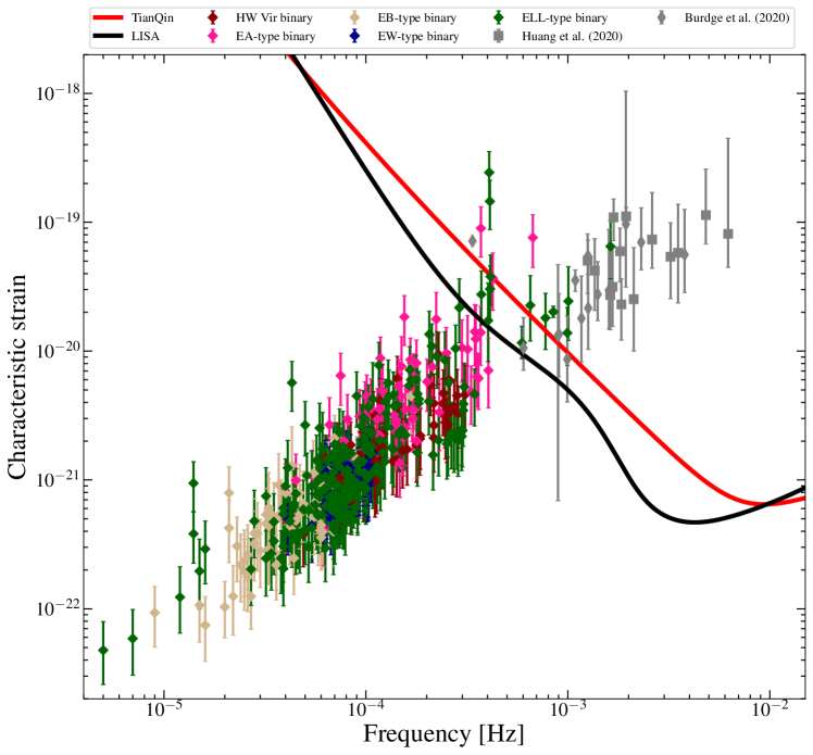
Figure 15: Characteristic gravitational-wave strain of the sources described in this work (shown as colors diamonds), compared with the samples of candidate verification binaries from Huang et al. (2020) (shown as grey squares) and Burdge et al. (2020a, b), Kilic et al. (2021) and Chandra et al. (2021) (shown as grey thin diamonds), overplotted with LISA sensitivity curve (solid black line) and TianQin sensitivity curve (solid red line).

6.4 GW Signals of Binary Systems

Galactic ultracompact binaries are the most numerous GW sources expected to be detected by future space-based GW detectors such as TianQin and LISA (Kupfer et al., 2018; Huang et al., 2020; Amaro-Seoane et al., 2022). The loudest signals can be detected individually, while a large number of the unresolved GW signals will superpose to form the DWDs foreground for the space-based GW detectors (Huang et al., 2020; Liang et al., 2022; Lu et al., 2022). Once the short-period DWDs candidates in our final catalog are confirmed, it can help to expand the population of verification binaries.

The GW radiation from DWDs can be considered as quasi-monochromatic signal sources, which can be described by seven parameters: frequency $f_{\mathrm{GW}}=2/P_{\mathrm{orb}}$, the dimensionless amplitude $\mathcal{A}$, ecliptic coordinates ($\lambda$, $\beta$), orbital inclination $\iota$, polarization angle $\Psi_{S}$, and initial orbital phase $\phi_{0}$ (Huang et al., 2020). The primary and secondary masses ($m_{1}$ and $m_{2}$), luminosity distance ($d$), and orbital period ($P_{\mathrm{orb}}$) of double white dwarfs can be derived from electromagnetic (EM) observations, and can be used to estimate the amplitude of the gravitational wave signal (Huang et al., 2020):

$$\mathcal{A}=\frac{2(G\mathcal{M})^{5/3}}{c^{4}d}(\pi f)^{2/3},$$ (13)

where $\mathcal{M}=(m_{1}m_{2})^{3/5}(m_{1}+m_{2})^{-1/5}$, $G$ and $c$ are the chirp mass, the gravitational constant and the speed of light, respectively.

The characteristic strain can be defined by the dimensionless GW amplitude $\mathcal{A}$ and the frequency of GW radiation $f_{\mathrm{GW}}$:

$$h_{c}=\sqrt{N_{\mathrm{cycle}}}\mathcal{A},$$ (14)

where $N_{\mathrm{cycle}}=f_{\mathrm{GW}}T_{\mathrm{obs}}$ is the number of binary orbital cycles observed during the mission, $T_{\mathrm{obs}}$ is the integration time (or observation time) of the detectors.

To estimate the SNR ($\rho$) of GW signals from DWDs, we use the expression defined as Korol et al. (2017) and Huang et al. (2020),

$$\rho^{2}=\frac{2\langle A^{2}\rangle T_{obs}}{\widetilde{S}_{n}(f_{s})},$$ (15)

and the average amplitude defined by

$$\left\langle A^{2}\right\rangle=\mathcal{A}^{2}\left[(1+\cos^{2}(\iota))^{2}\left\langle F^{2}_{+}\right\rangle+4\cos^{2}(\iota)\left\langle F^{2}_{\times}\right\rangle\right],$$ (16)

where $\left\langle F^{2}_{+}(\lambda,\beta,\Psi_{S})\right\rangle$ and $\left\langle F^{2}_{\times}(\lambda,\beta,\Psi_{S})\right\rangle$ are the orbit averaged detector responses (Cornish & Larson, 2003; Huang et al., 2020). $\widetilde{S}_{n}(f_{s})$ is the sensitivity curve of the detector in a Michelson channel. The sensitivity curve of TianQin can be expressed analytically as Eqs. (13) of Huang et al. (2020), and the sensitivity curve of the detector of LISA from Robson et al. (2019).

In order to estimate the SNR of binaries under the actual observation conditions of the detectors, we consider the effective observation time of the GW detectors. For TianQin, the 5-year mission adopts the observation mode of three-month observation plus three-month shutdown protection, which effectively corresponds to 2.5 years of observation time (Luo et al., 2016; Huang et al., 2020). For LISA, based on the performance of LISA Pathfinder, LISA Science Group expects that LISA will have a duty cycle of about 0.75, which means that in its 4-year mission, its effective observation time is 3 years (Amaro Seoane et al., 2022). In equation (15), the observation time $\rm T_{obs}$ of TianQin is set as 2.5 years, and that of LISA is set as 3 years.

In this work, we discovered 429 CWDB candidates. In order to calculate the SNR of these sources, we need to obtain the source parameters. The sky location ($\lambda,\beta$) of sources can be used the ecliptic longitude (ecl_lon) and ecliptic latitude (ecl_lat) from Gaia EDR3 data. Using BLS and CE to analyze the ZTF light curve, we can calculate the trustworthy orbital period of binary candidates. We compared the period values obtained by the two algorithms after independently calculating three groups of ZTF photometry data, and finally estimated the average orbital period and retained it to three decimal places. The luminosity distance can be determined using trigonometric parallaxes from Gaia EDR3 (Lindegren et al., 2021; Kupfer et al., 2018). See Table 3 for further details of potential GW candidates. We assume that the primary mass $m_{1}$ obeys a uniform distribution $U(0.5,0.7)$ $\mathrm{M}_{\odot}$, and the secondary mass $m_{2}$ obeys a uniform distribution $U(0.2,0.4)$ $\mathrm{M}_{\odot}$ according to Burdge et al. (2020b), and we fix $\iota=\pi/3$, $\Psi_{S}=\pi/2$ for all new candidates, since there are currently no measurements of these parameters.

We report the estimated TianQin/LISA SNR for the sources in the sample in Table 3. The first part of the Table 3 shows the first 24 candidates with periods less than 100 minutes in our binary sample, which are defined as potential GW candidates (for further details on their light curves, please see Appendix D). The later part of the Table 3 shows the recently discovered GW sources by other surveys that is not summarised in Huang et al. (2020). Figure 15 shows the characteristic strain of gravitational radiation of our newly discovered binary samples and other classic verification binaries and the sensitivity of TianQin and LISA. As illustrated in Figure 15, most sources of our sample fall below the sensitivity curves of TianQin and LISA, about 10 candidates fall above the LISA sensitivity curve, and about 16 candidates fall above the LISA sensitivity curve after 4 years of observations. In estimating the GW signals of candidates, we fixed some source parameters as constants, and the mass was uniformly distributed (we remark that for some binary systems this assumption might be unphysical), the current uncertainty in the SNR and GW amplitude of all sources originate from the uncertainty of distance measurement (mainly due to the standard error of parallax, parallax_error). In our binary sample, the light curve shapes of potential GW candidates located above or near the sensitivity curve are mainly EA-type and ELL-type binaries. We adopt a low SNR threshold of 5 as the minimum standard for GW signals detected by TianQin and LISA. For TianQin, we found two new candidates VBs, namely ZTF J0526+5934 (SNR $\sim 12$) and ZTF J2007+1742 (SNR $\sim 7$), plus other newly discovered GW sources in the later part of Table 3, bringing the total number of VBs to 18 for TianQin. For LISA, we found 6 new VBs candidates, bringing the total number of VBs to 31 for LISA.

Table 3: The sources parameter, amplitude $\mathcal{A}$ and SNR for 24 ultra-short period ($P_{\rm orb}\leq$ 100 min) potential GW candidates.

ZTF Name	$\lambda$	$\beta$	$f$	$d$	$\mathcal{A}$	SNR	SNR
	[deg]	[deg]	[mHz]	[kpc]	[$\times 10^{-23}$]	[TianQin]	[LISA]
ZTF J0526+5934	84.6989	36.2955	1.626	0.846	18.15	12.777	35.788
ZTF J1840-1742	279.7729	5.3797	1.006	1.345	8.66	3.297	5.439
ZTF J1707-1522	257.2883	7.4854	0.994	2.285	4.94	1.477	2.931
ZTF J2130+4420[b]	348.1685	54.4443	0.847	1.309	7.81	0.850	2.076
ZTF J2351+6305	36.8445	55.5895	0.775	1.286	7.32	0.681	2.409
ZTF J1611+6308	183.9169	78.0916	0.671	0.257	33.07	2.282	8.147
ZTF J1813+4251[e]	276.0031	66.2346	0.652	0.835	10.00	0.901	2.415
ZTF J2055+4651[b]	341.0544	59.9596	0.592	2.264	5.37	0.283	0.779
ZTF J1603+2150	232.8645	41.6031	0.425	0.309	20.11	0.667	2.489
ZTF J0451+0104	71.5240	-21.2702	0.414	0.294	20.96	0.924	2.568
ZTF J0112+5827	44.5245	45.8154	0.412	0.364	16.83	0.433	1.915
ZTF J2334+3921	12.6230	38.0721	0.411	0.076	80.71	2.374	9.624
ZTF J2007+1742	309.0298	36.9204	0.408	0.045	135.70	7.219	13.969
ZTF J1810-2138	272.3779	1.7778	0.404	1.683	3.97	0.217	0.513
ZTF J1705+3455	249.0813	57.3809	0.403	0.616	9.68	0.309	1.047
ZTF J1943-2657	293.0642	-5.5741	0.373	0.358	16.05	0.814	1.615
ZTF J1708-2548	258.3723	-2.8898	0.371	0.109	52.53	2.042	5.605
ZTF J1948+5250	327.3373	70.9334	0.370	0.699	8.17	0.208	0.721
ZTF J1944+5449	329.5948	72.8635	0.361	1.552	3.64	0.085	0.306
ZTF J1927+3411	302.7131	55.1734	0.356	1.482	3.78	0.121	0.320
ZTF J0609+3652	91.8999	13.4434	0.350	0.733	7.49	0.288	0.705
ZTF J1100+5210	142.3087	41.4823	0.346	0.636	8.57	0.259	0.655
ZTF J0050+2551	21.9928	18.7691	0.345	1.963	2.81	0.051	0.242
ZTF J1622+4730	224.3785	67.1495	0.332	1.814	2.98	0.050	0.212
ZTF J2243+5242[a]	13.2423	53.9599	3.788	1.753	10.26	19.992	78.739
ZTF J0538+1953[b]	84.8061	-3.4356	2.308	0.997	16.38	18.915	75.532
ZTF J1905+3134[b]	293.7825	53.6335	1.938	0.696	24.78	26.305	79.343
ZTF J2029+1534[b]	314.4631	33.4205	1.597	1.095	8.36	4.743	9.144
ZTF J0722-1839[b]	115.8782	-40.2164	1.406	1.267	8.29	3.451	6.666
ZTF J1749+0924[b]	267.0209	32.8576	1.261	1.291	6.85	2.178	4.685
ZTF J2228+4949[b]	7.0683	53.2065	1.167	2.076	5.92	1.520	4.416
ZTF J1946+3203[b]	307.9775	52.0541	0.993	1.919	3.09	0.626	1.186
ZTF J0643+0318[b]	101.5702	-19.6948	0.903	2.040	5.08	1.519	2.398
ZTF J0640+1738[b]	99.6432	-5.4567	0.894	1.576	4.97	1.339	2.262
ZTF J2320+3750[b]	8.7171	38.0936	0.603	1.256	4.85	0.244	0.793
SDSS J0634+3803[c]	97.0832	14.8390	1.257	0.433	17.36	13.782	23.919
SMSS J0338-8139[c]	286.4357	-72.7068	1.089	0.536	12.11	2.199	6.226
SDSS J1337+3952[d]	182.8931	45.5716	0.337	0.114	43.86	1.151	5.030

Note. — The position ($\lambda$, $\beta$) are the ecliptic coordinates, $f$ is the GW frequency, $\mathcal{A}$ is the dimensionless amplitude, $d$ is the luminosity distance.

7 Conclusion

In this work, we have presented a catalog of short-period close white dwarf binary candidates based on the Gaia EDR3 catalog and the Zwicky Transient Facility photometry data. We defined a color-cutting criterion for selecting initial samples in the Gaia H-R diagram. In the Gaia EDR3 data, we searched 823231 high signal-to-noise ratio sources after using quality filtering parameters (Pelisoli & Vos, 2019; Geier et al., 2019). We applied the Gaia variability metric (Guidry et al., 2021) to select 12480 most variable objects with high confidence from high-SNR samples.

We cross-matched the high-confidence variable source catalog with time-domain photometry data of the ZTF Public DR8 and analyzed the light curves of all variable sources. After analyzing the ZTF light curves, a total of 826 candidates were identified to have distinguishable periodic variability. Taking the shape of the light curve produced by the eclipse process of the binary system as the selection criterion, we found 429 binary candidates. The final catalog includes 58 HW Vir-type binaries, 65 EA-type binaries, 56 EB-type binaries, 41 EW-type binaries, and 209 ELL-type binaries.

We analyzed four short-period close white dwarf binary candidates with special light curves in the final catalog. ZTF J2351+6305 is an ellipsoidal variable binary with a period of less than 60 minutes ($\mathrm{P}_{\mathrm{orb}}$ = 42.985 min), which is similar to a mass-transferring and recently-detached CV (El-Badry et al., 2021b). ZTF J1611+6308 is a deeply-eclipsing white dwarf binary with an orbital period of 49.708 minutes. ZTF J1813+4251 is a short-period ($\mathrm{P}_{\mathrm{orb}}$ = 51.161 min) binary candidate near the classical-CV in the Gaia H-R diagram. ZTF J0112+5827 is a CV candidate similar to an eclipsing polar BS tri system (Kolbin et al., 2022) with a period of 80.912 minutes. We obtained the ZTF photometric data of these special candidates and analyzed their positions in the Gaia H-R diagram. The future follow-up observation of the spectra can be used to estimate the physical parameters such as masses, temperatures, and radial velocity semiamplitudes. The high-speed photometric observation can be used to solve the orbital parameters of the binary system, such as radius, inclination, semimajor axis, and orbital period.

We define the distribution of the Gold samples of close-WD binaries based on the sub-classes of stars in the Gaia H-R diagram. In the final catalog, a total of 429 close-WD binary candidates were divided into 85 PCEB Gold samples, 224 CV Gold samples, 45 ELM-WD Gold samples, and 11 DWD Gold samples.

We estimated the gravitational wave amplitudes and signal-to-noise ratios of all candidates in our binary sample. We found that we have two potential GW candidates with SNRs greater than 5 in the 2.5-year observation time of TianQin, which increases the total number of candidate VBs for TianQin to 18. For LISA, we have six new sources with SNRs of more than 5 in their 3-year effective observation time with a total of 4-year mission lifetime. The total number of LISA VBs has reached 31.

In future work, we aim to use multi-band spectral energy distribution to analyze the compositions and obtain the effective temperature and surface gravity of the binary systems to study their evolution process. We also plan to use LAMOST spectral and jointly fit the light curve to obtain the physical parameters and orbital parameters for our binary candidates to confirm their binary nature.

Appendix A Gaia astrometric query cut

Below we show the initial-cut selection criteria applied to Gaia EDR3 data through the following Astronomical Data Query Language (ADQL) query. Our ADQL query jobs are run in the Gaia@AIP services or ARI’s Gaia services.

⬇

SELECT *

FROM gaiaedr3.gaia_source

WHERE dec > -28.0

AND bp_rp < 1.0

AND parallax_over_error > 5

AND phot_bp_mean_flux_over_error > 10

AND phot_rp_mean_flux_over_error > 10

AND 5 + 5 * log10((parallax + 0.029)/1000) + phot_g_mean_mag > 3.7 * bp_rp + 2.2

AND 5 + 5 * log10((parallax + 0.029)/1000) + phot_g_mean_mag < 2.7 * bp_rp + 11.5

AND phot_bp_rp_excess_factor < 1.45 + 0.06 * power(phot_bp_mean_mag - phot_rp_mean_mag, 2)

AND phot_bp_rp_excess_factor > 1.0 + 0.015 * power(phot_bp_mean_mag - phot_rp_mean_mag, 2)

AND (astrometric_chi2_al / (astrometric_n_good_obs_al - 5) < 1.44

OR astrometric_chi2_al / (astrometric_n_good_obs_al - 5) < 1.44 * exp(- 0.4 * (phot_g_mean_mag - 19.5)));

Below we show the Gaia Variability cut selection criteria using the following ADQL query:

⬇

SELECT *

FROM gaiaedr3.gaia_source

WHERE dec > -28.0

AND bp_rp < 1.0

AND parallax_over_error > 5

AND phot_bp_mean_flux_over_error > 10

AND phot_rp_mean_flux_over_error > 10

AND 5 + 5 * log10((parallax + 0.029)/1000) + phot_g_mean_mag > 3.7 * bp_rp + 2.2

AND 5 + 5 * log10((parallax + 0.029)/1000) + phot_g_mean_mag < 2.7 * bp_rp + 11.5

AND phot_bp_rp_excess_factor < 1.45 + 0.06 * power(phot_bp_mean_mag - phot_rp_mean_mag, 2)

AND phot_bp_rp_excess_factor > 1.0 + 0.015 * power(phot_bp_mean_mag - phot_rp_mean_mag, 2)

AND (astrometric_chi2_al / (astrometric_n_good_obs_al - 5) < 1.44

OR astrometric_chi2_al / (astrometric_n_good_obs_al - 5) < 1.44 * exp(- 0.4 * (phot_g_mean_mag - 19.5)))

AND phot_g_mean_flux_error * power(phot_g_n_obs, 0.5) / phot_g_mean_flux - ((8.31e-9) * exp(0.794 * phot_g_mean_mag) + 0.0005 * exp(phot_g_mean_mag - 17.0) + 0.019) > 0.0;

Appendix B Short-period CWDBs catalogs

Below we show the Gaia photometric parameters and the orbital period parameters for all 429 objects in our binary sample. According to the types of the light curve, we can divide them into five tables: HW Vir-type binary candidates (see Table 4), EA-type binary candidates (see Table 5), EB-type binary candidates (see Table 6), EW-type binary candidates (see Table 7), and ELL-type binary candidates (see Table 8).

Table 4: HW Vir-type binary candidates

ZTF Name	Gaia EDR3	RA	Dec	$\varpi$	G	$G_{\mathrm{BP}}-G_{\mathrm{RP}}$	$G_{\mathrm{abs}}$	$P_{\mathrm{orb}}$	$\mathcal{A}$
	sourceID	(deg)	(deg)	(mas)	(mag)	(mag)	(mag)	(min)	($\times 10^{-23}$)
ZTF J2040+3407	1864121982365984128	310.19402	34.11743	0.55	17.41	0.42	6.14	107.543	2.94
ZTF J2345+5057	1943858286426802304	356.26684	50.96520	0.43	16.43	-0.13	4.62	116.686	2.18
ZTF J2120+4014	1965596391525733120	320.17691	40.24297	0.62	17.02	0.25	5.99	117.598	3.02
ZTF J0718+0739	3154801672464733440	109.74027	7.65367	0.52	15.22	-0.41	3.82	121.625	2.51
ZTF J0836-0802	5753841281270433536	129.05426	-8.03995	0.51	15.28	-0.37	3.81	127.971	2.35
ZTF J2328+6415	2209063896962507520	352.22684	64.26275	0.53	17.37	0.91	5.99	128.107	2.47
ZTF J2046+5147	2182023160826160000	311.65906	51.79319	0.93	15.22	0.18	5.07	129.086	4.19
ZTF J0518-2308	2961366588952039552	79.52903	-23.14588	0.42	15.89	-0.35	3.97	131.287	1.91
ZTF J0827-2736	5646693014160460416	126.95875	-27.61052	0.38	16.86	-0.18	4.78	132.154	1.82
ZTF J0113+2257[1]	2791084432881749760	18.41288	22.96084	0.42	16.61	-0.38	4.74	134.457	2.00
ZTF J0729-1837	3026543267432558336	112.27269	-18.61764	0.51	15.91	0.19	4.44	135.012	2.24
ZTF J0710+6655	1102107819544067456	107.67521	66.92872	0.79	14.62	-0.36	4.10	137.731	3.41
ZTF J0820+0008[2][3]	3077510098136276480	125.22307	0.14541	0.66	15.15	-0.35	4.25	138.586	2.84
ZTF J1338-0201	3637481302758519040	204.70058	-2.03039	1.68	13.36	-0.40	4.49	145.463	6.98
ZTF J0405+5044	250657727370153472	61.34537	50.73949	0.73	17.45	0.99	6.77	153.322	3.00
ZTF J0016+7855	564551735705888384	4.15468	78.92195	0.38	16.53	-0.17	4.46	153.782	1.62
ZTF J1848+1157	4504497623459700992	282.19609	11.95561	0.49	16.69	0.06	5.14	153.837	2.03
ZTF J2234+2456[3]	1877320760449993216	338.58958	24.94919	1.08	14.16	-0.36	4.35	159.246	4.24
ZTF J2006+0416	4247741141287799680	301.71988	4.270338	0.49	16.22	-0.13	4.68	179.658	1.82
ZTF J2025-1200	6880002734442865920	306.40622	-12.00433	0.44	16.32	-0.36	4.56	180.145	1.73
ZTF J2131+4654[4]	1978219536621659136	322.92266	46.90833	0.39	17.38	0.07	5.39	187.154	1.56
ZTF J2100-1411	6888269309535155456	315.07248	-14.19017	0.44	16.55	-0.31	4.76	208.848	1.54
ZTF J1922+2624	2025568909688842112	290.67035	26.40430	0.44	17.63	0.41	5.86	218.801	1.54
ZTF J2318+8232	2287403962995179264	349.67784	82.53852	0.38	16.89	-0.09	4.79	226.186	1.26
ZTF J2315+5828	2010408220561381632	348.84423	58.48000	0.66	17.61	0.87	6.72	228.536	2.11
ZTF J1852-2147[5]	4078817195637328256	283.07503	-21.79744	1.12	13.75	-0.16	3.99	231.945	3.41
ZTF J1533+3759[6]	1375814952762454272	233.45602	37.99106	1.90	12.94	-0.38	4.34	232.949	5.78
ZTF J0724-2110	5619901038222784768	111.12425	-21.17284	0.40	17.53	0.24	5.56	235.387	1.36
ZTF J2118+4047	1968673301791825920	319.55255	40.79099	0.44	16.71	0.05	4.95	245.292	1.35
ZTF J1852+1445	4507223312777873280	283.03169	14.76307	0.85	14.99	0.24	4.65	274.199	2.32
ZTF J1840+0703	4286518927853983360	280.17673	7.05606	0.58	16.39	0.25	5.23	275.205	1.62
ZTF J2146+6616	2219505890166498048	326.73603	66.26855	0.68	16.21	0.37	5.37	278.565	1.84
ZTF J1849-1340	4102198997623267456	282.46445	-13.67621	1.62	14.36	0.42	5.41	285.042	4.31
ZTF J0626-0250	3117155669938231552	96.62394	-2.84625	0.54	16.01	0.04	4.65	286.257	1.45
ZTF J2035+3544	2056653885784893952	308.89592	35.73469	0.72	16.46	0.52	5.74	294.433	1.88
ZTF J2025+5851	2188514226495429632	306.31183	58.85225	0.38	17.53	0.13	5.46	295.608	1.12
ZTF J0753+7224	1110899853820753792	118.37031	72.40680	0.38	16.48	-0.21	4.35	299.884	1.05
ZTF J1838+0500	4283927443344408960	279.58508	5.00373	0.57	17.42	0.66	6.21	302.844	1.53
ZTF J2326+1230	2812551023024830720	351.71862	12.50606	1.39	14.33	-0.17	5.04	305.145	3.52
ZTF J1939+1110	4303030190905072640	294.76892	11.18227	0.81	14.86	-0.14	4.41	306.883	2.05
ZTF J0910+7810	1131845039229607680	137.58201	78.17318	0.40	16.14	-0.32	4.16	337.571	1.00
ZTF J2240+5437	2003241230122936064	340.21327	54.63084	0.70	14.98	0.01	4.21	339.664	1.66
ZTF J2111+3325	1866796475676061056	317.98098	33.43218	0.78	15.36	-0.22	4.82	356.308	1.79
ZTF J1906-0051	4262586854711451904	286.55537	-0.85630	0.79	15.73	0.25	5.22	358.359	1.80
ZTF J2058+3604	1869815700251723392	314.51502	36.08310	0.46	16.34	0.02	4.64	360.352	1.06
ZTF J2004+1411	1806486197003559040	301.04835	14.19727	0.48	16.86	-0.18	5.26	369.263	1.13
ZTF J1830+4331	2111853428244955264	277.71017	43.52205	0.38	16.16	-0.37	4.05	389.899	0.85
ZTF J0519-1916	2969438206889996160	79.94864	-19.28166	1.08	13.59	-0.35	3.75	395.409	2.30
ZTF J2045+3200	1862846132257229312	311.35609	32.00379	0.69	17.26	0.91	6.46	400.113	1.49
ZTF J2025+4247	2068952271239193344	306.28696	42.79075	0.99	15.06	-0.05	5.05	421.206	2.03
ZTF J1859+0751	4307083884080817792	284.85281	7.85063	1.26	15.61	0.51	6.11	428.491	2.55
ZTF J1940+0421	4290201742045065344	295.02546	4.35965	0.54	16.31	-0.05	4.96	444.643	1.08
ZTF J1630+1801	4467130720760209152	247.68937	18.02232	0.63	15.37	-0.27	4.36	445.391	1.25
ZTF J2226+6159	2202073408192045056	336.63336	61.98438	0.68	17.05	0.96	6.22	447.947	1.35
ZTF J0441+1636	3310121300640873984	70.47707	16.61040	1.21	15.42	0.59	5.83	447.968	2.38
ZTF J2036+2350	1819387836386252672	309.11556	23.83959	0.41	16.96	-0.07	5.04	518.007	0.79
ZTF J0808+3202	901929564359845888	122.11083	32.04179	1.21	13.78	-0.32	4.18	532.411	2.11
ZTF J1831+2656	4585381817643702528	277.82745	26.93670	0.40	14.96	-0.23	2.99	679.287	0.61

Note. — The coordinates and basic photometric characteristics of the 58 HW Vir-type binary candidates discovered so far using ZTF data. Coordinates are taken from Gaia and are in J2000.0. The IAU name is provided in the catalog.

Table 5: EA-type binary candidates

ZTF Name	Gaia EDR3	RA	Dec	$\varpi$	G	$G_{\mathrm{BP}}-G_{\mathrm{RP}}$	$G_{\mathrm{abs}}$	$P_{\mathrm{orb}}$	$\mathcal{A}$
	sourceID	(deg)	(deg)	(mas)	(mag)	(mag)	(mag)	(min)	($\times 10^{-23}$)
ZTF J1611+6308	1629388752470472704	242.89152	63.14213	3.89	18.28	0.19	11.24	49.708	33.07
ZTF J1603+2150	1206052590817661696	240.89972	21.84231	3.23	19.11	0.19	11.66	78.394	20.11
ZTF J1810-2138	4093796151752232192	272.55704	-21.64038	0.62	17.54	0.72	6.51	82.426	3.97
ZTF J1708-2548	4111991385628196224	257.07942	-25.80907	9.21	15.36	0.62	10.19	89.896	52.53
ZTF J1948+5250	2137193078157620480	297.08732	52.84653	1.43	18.50	0.53	9.28	90.134	8.17
ZTF J1944+5449	2138663782338254464	296.17858	54.82857	0.64	15.75	-0.23	4.79	92.393	3.64
ZTF J1927+3411	2046661975094606208	291.90956	34.19492	0.67	15.26	-0.31	4.41	93.522	3.78
ZTF J0609+3652[1]	3453995450857025664	92.30994	36.86744	1.36	18.79	-0.03	9.47	95.105	7.49
ZTF J1100+5210[1][2]	836510989033113472	165.18813	52.17878	1.57	18.52	-0.24	9.51	96.310	8.57
ZTF J1622+4730[3]	1410860511508492288	245.73608	47.51419	0.55	16.21	-0.40	4.93	100.496	2.98
ZTF J1844+4857[1]	2119978952315202176	281.14332	48.96011	1.26	19.29	0.25	9.79	104.644	6.52
ZTF J2037+2616	1855919930550745856	309.39423	26.28245	1.39	18.58	0.65	9.31	111.585	6.91
ZTF J0612-1911	2941800362921100928	93.14276	-19.18675	1.56	18.05	-0.29	9.03	133.506	6.85
ZTF J1502+4754	1588999361055110656	225.54484	47.91520	1.91	19.29	0.42	10.69	137.685	-
ZTF J2204+5016	1976934104452780928	331.09721	50.27252	0.55	18.11	0.73	6.82	144.184	2.48
ZTF J0102-0553	2524831503167265664	15.51027	-5.89828	3.30	18.90	0.68	11.49	149.372	13.34
ZTF J2216+1059	2724510992389846784	334.12713	10.99822	1.48	18.29	0.21	9.15	156.508	5.82
ZTF J0703+1018	3158071830502039424	105.82180	10.30901	1.21	14.64	0.18	5.05	165.584	4.60
ZTF J2053+4721	2166852992748641024	313.43919	47.35499	0.59	17.61	0.89	6.48	172.110	1.42
ZTF J2159+4954	1979538194664660608	329.76835	49.90843	0.44	17.63	0.51	5.85	186.423	1.68
ZTF J1905+3015	2040949943465818880	286.33086	30.25680	0.87	15.91	0.33	5.62	186.757	3.07
ZTF J1552+1254	1191504471436192512	238.23369	12.91208	1.94	16.53	-0.21	7.97	187.316	6.82
ZTF J1810+1735	4526200711655400064	272.71578	17.59947	1.08	16.26	0.64	6.43	194.175	3.69
ZTF J1015-0308	3828660708104028032	153.78902	-3.14249	1.61	14.37	0.23	5.40	194.311	5.52
ZTF J0413+3116[4]	166065705072038144	63.37181	31.27451	0.74	16.84	0.536	6.19	194.894	2.57
ZTF J2038+3605	2062662892933692416	309.50297	36.09175	1.21	16.37	0.67	6.79	197.026	4.12
ZTF J0756+0858	3146975005100167296	119.22131	8.97549	0.89	16.88	0.37	6.65	197.243	3.06
ZTF J1913+1218	4313192495850348544	288.47720	12.30087	2.24	14.30	0.63	6.05	201.154	7.50
ZTF J0506+7306[2]	502209190190665856	76.64026	73.11295	1.34	18.62	0.40	9.26	203.760	4.44
ZTF J1900+2921	2040790582998889344	285.14209	29.35925	0.98	16.36	0.54	6.32	211.979	3.17
ZTF J2001+4823	2086158112083513728	300.32986	48.38386	0.67	18.49	0.83	7.64	212.716	2.27
ZTF J1920+2722[1]	2025873096433233664	290.05891	27.37168	5.22	15.56	0.31	9.15	215.089	16.67
ZTF J1934+0202	4288094214457507968	293.59654	2.04795	0.62	17.54	0.82	6.49	218.219	2.06
ZTF J1910+2917	2039098258506802560	287.60865	29.28664	0.57	18.01	0.56	6.78	218.251	1.93
ZTF J0417+2215	52564077511652992	64.35303	22.25617	2.27	19.13	0.76	10.91	221.733	7.00
ZTF J0822+5105[5]	1028258463932870656	125.65013	51.09010	1.33	15.16	0.42	5.78	224.461	4.13
ZTF J1820-1227	4152844148118986752	275.16223	-12.46033	0.74	17.01	0.86	6.35	225.896	2.35
ZTF J2137+4346	1967765006407778688	324.48352	43.77767	0.74	17.74	0.88	7.09	227.310	2.33
ZTF J2054+3203	1865673904360821760	313.73837	32.06127	1.65	18.56	0.97	9.64	230.023	5.03
ZTF J1832+1016	4480616299611285888	278.11749	10.28174	0.92	15.92	0.54	5.74	235.698	2.77
ZTF J0638+0202	3126748732793713024	99.63705	2.03539	0.71	17.95	0.71	7.19	236.098	2.24
ZTF J2023+4631	2083145484587589632	305.87717	46.52484	0.86	16.54	0.83	6.22	237.223	2.59
ZTF J2011+2818	1837207896220382464	302.98296	28.30309	1.03	16.13	0.76	6.19	240.853	3.06
ZTF J1408+2950[2]	1453111749770736256	212.19651	29.84578	1.85	18.64	0.08	9.98	276.182	4.99
ZTF J0107+4845[6]	401879681868136704	16.92848	48.75519	1.31	15.06	0.47	5.65	278.779	3.53
ZTF J1336+5154	1559987685901122304	204.17034	51.91381	3.43	12.93	0.26	5.60	283.207	9.13
ZTF J0805-1430	5725000709020309120	121.42908	-14.51009	1.39	18.39	0.33	9.12	285.362	3.69
ZTF J0453+2246	3413226556129600640	73.25209	22.78167	0.85	17.72	0.95	7.37	285.901	2.30
ZTF J0033+3855[2]	380560941677424768	8.46929	38.92489	1.19	18.34	-0.18	8.71	291.877	3.11
ZTF J2230+5108	2000300410171107072	337.51890	51.14879	0.64	17.10	0.72	6.15	305.884	1.65
ZTF J0900+4348	1009242620785138688	135.09604	43.80374	1.57	18.35	-0.14	9.34	313.462	3.90
ZTF J2256+5954[7]	2014349389931360768	344.03533	59.90837	2.06	14.50	0.68	6.08	329.188	4.98
ZTF J2308+6125[2]	2014898802148215424	347.11902	61.42704	1.53	19.41	0.85	10.34	336.029	3.60
ZTF J0630+4147	958364128959466624	97.60905	41.79843	1.60	18.11	0.07	9.13	357.030	3.64
ZTF J1937+3132	2033181618967776128	294.44152	31.54854	0.47	17.45	0.72	5.80	397.662	1.06
ZTF J0344+0930	12007117949000576	56.08404	9.50189	0.87	18.05	0.31	7.74	404.152	1.86
ZTF J0045+5034	414813439007636352	11.25983	50.56896	1.79	17.59	-0.07	8.88	412.675	3.72
ZTF J0429+3447[2]	173280902235344640	67.48047	34.79279	4.24	17.01	0.69	10.15	442.304	8.39
ZTF J2226+5604	2007483141676822400	336.67699	56.06759	2.06	18.98	0.96	10.55	504.257	3.71
ZTF J1841-1759	4098680938387190272	280.42020	-17.98867	0.82	16.68	0.91	6.26	522.377	1.47
ZTF J1712+3218	1334339278219282944	258.09192	32.31564	0.29	16.98	0.53	4.29	537.598	0.59
ZTF J1756-0341	4177449504661490432	269.12620	-3.69917	1.04	16.61	0.99	6.69	612.964	1.66
ZTF J0821+4559	930093722208184448	125.43870	45.98982	1.18	17.43	-0.06	7.79	733.110	1.67
ZTF J1746-0309	4176942419339829504	266.52469	-3.16626	1.21	15.98	0.60	6.41	825.804	1.58
ZTF J1831+0509	4284322756446267264	277.76258	5.16490	0.67	17.00	0.85	6.13	826.980	0.89

Note. — The coordinates and basic photometric characteristics of the 65 EA-type binary candidates discovered so far using ZTF data. Coordinates are taken from Gaia and are in J2000.0. The IAU name is provided in the catalog.

Table 6: EB-type binary candidates

ZTF Name	Gaia EDR3	RA	Dec	$\varpi$	G	$G_{\mathrm{BP}}-G_{\mathrm{RP}}$	$G_{\mathrm{abs}}$	$P_{\mathrm{orb}}$	$\mathcal{A}$
	sourceID	(deg)	(deg)	(mas)	(mag)	(mag)	(mag)	(min)	($\times 10^{-23}$)
ZTF J2044+2653	1856208999031665664	311.19562	26.88862	1.15	18.74	0.69	9.05	199.497	3.90
ZTF J1301+1631	3937384472308048256	195.44488	16.52939	0.77	14.52	0.47	3.95	369.066	1.72
ZTF J0515+0104	3233813338246568448	78.92258	1.07789	1.52	15.73	0.97	6.65	478.965	2.86
ZTF J1716+7325	1655226867702084352	259.09056	73.42544	0.25	16.39	0.32	3.39	479.665	0.54
ZTF J0101-1952	2356059083939929344	15.39862	-19.87515	0.40	15.49	0.36	3.49	494.834	0.75
ZTF J0734-0406	3057327664560134144	113.65574	-4.11209	0.89	16.89	0.91	6.64	511.579	1.62
ZTF J2241+4639	1983499150940152064	340.35358	46.65429	0.73	17.94	0.81	7.24	542.995	1.31
ZTF J0324-0715	5168804986809073280	51.16995	-7.26322	0.29	16.23	0.29	3.54	548.786	0.57
ZTF J1230+6630	1680749247001917184	187.74306	66.51525	0.29	15.54	0.24	2.87	554.534	0.52
ZTF J0247-0704	5177657605896269312	41.79151	-7.06765	0.34	16.33	0.51	3.97	556.498	0.65
ZTF J2123-2258	6827891999317461760	320.88565	-22.96811	0.48	16.02	0.62	4.43	562.538	0.84
ZTF J1754+0755	4475982678420172416	268.73763	7.92054	0.39	17.03	0.75	4.98	563.297	0.73
ZTF J0712+0801	3153629597367436032	108.07661	8.02424	0.33	16.47	0.53	4.09	573.109	0.62
ZTF J2337+4222	1925364058466959872	354.39167	42.38158	0.62	15.99	0.63	4.95	581.149	1.03
ZTF J0643+2016	3377801803311816832	100.83036	20.27626	0.53	16.78	0.89	5.39	593.545	0.89
ZTF J0344+2444	69807413427563648	56.20413	24.74559	1.05	17.57	0.83	7.68	603.091	1.71
ZTF J2159+4841	1976417265265163264	329.91645	48.69451	0.44	17.85	0.97	6.05	603.543	0.78
ZTF J0217+4837	354932047187323136	34.44003	48.62936	0.52	16.61	0.78	5.19	665.930	0.53
ZTF J1854-1727	4086972543941116800	283.52717	-17.45326	0.67	17.21	0.97	6.35	679.363	1.05
ZTF J0201+4648	356034616834644352	30.27649	46.80116	0.88	16.42	0.58	6.16	703.371	1.30
ZTF J1055-0737	3763605388227660800	163.90577	-7.62389	0.69	14.23	0.35	3.44	711.975	1.00
ZTF J2043+2306	1818322066019513600	310.86748	23.11365	0.60	16.47	0.74	5.36	712.524	0.89
ZTF J0520-1453	2984872498285670272	80.08871	-14.88989	0.53	17.07	0.57	5.69	732.686	0.81
ZTF J1304+0825	3731034005522686976	196.11280	8.42102	0.29	16.17	0.33	3.54	746.199	0.30
ZTF J0753-0012	3082695772931676288	118.25777	-0.20069	0.25	16.37	0.33	3.38	753.151	0.42
ZTF J1701-2247	4113892784798158336	255.32855	-22.79002	1.67	18.97	0.99	10.08	776.341	2.23
ZTF J0128+4804	399890218656241024	22.04907	48.07493	0.51	16.17	0.69	4.696	796.607	0.74
ZTF J0311+3734	139485973542872704	47.87895	37.57813	1.09	15.97	0.99	6.16	837.375	1.41
ZTF J2002+1802	1822026320711502336	300.61449	18.04746	0.78	16.97	0.84	6.44	868.189	1.02
ZTF J2008+2104	1829610133445224320	302.13996	21.07196	0.78	17.00	0.92	6.47	884.481	1.00
ZTF J1655-2724	6033448733189239424	253.76696	-27.40550	1.371	18.25	0.81	8.94	900.927	1.69
ZTF J2108+3342	1867030396774731264	317.08629	33.71471	0.28	16.96	0.60	4.24	919.922	0.41
ZTF J2343+4132	1922033809544560256	355.93942	41.53877	0.37	17.13	0.65	4.94	938.066	0.50
ZTF J2040+2458	1843500087722545024	310.15486	24.96964	0.80	18.29	0.88	7.82	944.735	0.99
ZTF J0643-0813	3098824779580917504	100.88082	-8.22560	0.97	17.46	0.98	7.39	998.508	1.13
ZTF J0649+1735	3358509639149090816	102.27923	17.58631	0.74	14.39	0.37	3.75	1000.318	0.86
ZTF J0820-2631	5693621781036383232	125.00209	-26.52507	0.47	17.01	0.51	5.39	1012.718	0.57
ZTF J2016-0652	4217070367505811584	304.00437	-6.88272	1.04	17.86	0.64	7.94	1018.327	1.19
ZTF J0816-1910	5707573350935814016	124.13182	-19.18219	0.79	16.74	0.95	6.25	1033.149	0.91
ZTF J0755-2548	5602163239921936640	118.81374	-25.81455	0.96	16.15	0.79	6.06	1050.289	1.07
ZTF J1009-1813	5672508546441496064	152.31721	-18.22504	0.50	16.21	0.52	4.72	1125.002	0.58
ZTF J1851-1736	4098893380295745536	282.79944	-17.61324	0.74	17.30	0.69	6.66	1140.925	0.80
ZTF J0737+0408	3137928983639894656	114.42192	4.13755	0.63	17.41	0.50	6.39	1195.982	0.68
ZTF J1854-1104	4202152846578981376	283.59711	-11.07917	0.78	17.09	0.98	6.55	1206.936	0.82
ZTF J1832+3700	2096186074741452416	278.10394	37.01439	0.24	16.03	0.21	2.89	1212.353	0.27
ZTF J1106-1543	3562570682205430400	166.54727	-15.71694	0.35	16.37	0.53	4.09	1274.879	0.39
ZTF J0341+0110	3269977340835567616	55.40700	1.17434	0.57	17.16	0.87	5.93	1288.509	0.58
ZTF J0115+5733	413444654415313024	18.83419	57.55689	0.43	17.26	0.69	5.41	1351.007	0.44
ZTF J0735-0548	3056824401771669248	113.80979	-5.80214	0.50	16.42	0.72	4.92	1369.928	0.50
ZTF J1725+0723	4490107249605958528	261.39886	7.39795	0.79	16.39	0.72	5.87	1446.636	0.72
ZTF J1839+2126	4531853163501651840	279.83683	21.44776	1.23	17.72	0.72	8.17	1578.550	1.04
ZTF J0518+5352	266380159532195072	79.62807	53.87206	2.31	18.52	-0.06	10.34	1580.644	1.95
ZTF J1432+4911	1603405235417939584	218.23784	49.19526	0.29	15.67	0.27	3.05	1686.030	0.26
ZTF J2310-0705	2631464168053997056	347.58333	-7.09853	0.28	15.67	0.24	2.90	2150.021	0.21
ZTF J1919+3307	2049149959447866368	289.91089	33.13277	0.42	17.31	0.64	5.42	2220.154	0.31
ZTF J1252+7348	1691332832397541376	193.11743	73.80680	0.73	16.28	0.81	5.59	3750.267	0.35

Note. — The coordinates and basic photometric characteristics of the 56 EB-type binary candidates discovered so far using ZTF data. Coordinates are taken from Gaia and are in J2000.0. The IAU name is provided in the catalog.

Table 7: EW-type binary candidates

ZTF Name	Gaia EDR3	RA	Dec	$\varpi$	G	$G_{\mathrm{BP}}-G_{\mathrm{RP}}$	$G_{\mathrm{abs}}$	$P_{\mathrm{orb}}$	$\mathcal{A}$
	sourceID	(deg)	(deg)	(mas)	(mag)	(mag)	(mag)	(min)	($\times 10^{-23}$)
ZTF J0825+4329	916342443812848000	126.31920	43.49201	0.69	16.08	0.86	5.29	309.922	1.76
ZTF J1236+2834	4010630775855198848	189.08203	28.56893	0.52	16.77	0.68	5.37	314.220	1.37
ZTF J1141+5713	845729741196604544	175.40832	57.22566	0.41	17.71	0.97	5.77	322.677	1.12
ZTF J0331+0207	3268078209375996288	52.96629	2.11906	0.38	17.04	0.77	4.97	323.731	1.05
ZTF J0929+3410	797507570680645888	142.26295	34.16816	0.66	17.05	0.95	6.14	324.423	1.66
ZTF J1452-0117	3650361600441639040	223.12124	-1.28868	0.52	17.09	0.89	5.68	324.529	1.34
ZTF J1007-2331	5665664881129095040	151.79161	-23.52445	0.38	16.55	0.53	4.45	325.688	1.00
ZTF J2203+1624	1775594696266837888	330.90915	16.40823	0.39	16.82	0.72	4.78	333.263	1.03
ZTF J0939+5317	1020477327518306176	144.89409	53.29758	0.46	17.39	0.91	5.71	335.634	1.18
ZTF J2210-2231	6819297593664167680	332.63002	-22.53291	0.65	16.71	0.95	5.76	338.301	1.56
ZTF J1003-2021	5670630584877219456	150.81417	-20.35720	0.55	16.73	0.75	5.45	344.530	1.33
ZTF J1303-1416	3524873445010500992	195.75769	-14.27026	0.61	16.82	0.97	5.75	345.065	1.46
ZTF J1649+2307	4566397516733907200	252.48514	23.12869	0.48	17.07	0.89	5.49	356.632	1.15
ZTF J1057-2320	3549023324562306432	164.36934	-23.34196	0.53	17.46	0.99	6.10	356.771	1.32
ZTF J1624+4949	1423341274153725952	246.22699	49.81761	0.49	17.96	0.96	6.45	367.421	1.20
ZTF J0640+2540	3384807444726636160	100.18558	25.68297	0.69	17.56	0.90	6.77	395.228	1.55
ZTF J2111+4809[1]	2165295912482637312	317.90238	48.15052	0.64	18.41	0.99	7.45	402.080	1.42
ZTF J1230+1848	3947827118353402240	187.71592	18.80951	0.79	17.09	0.97	6.59	417.447	1.68
ZTF J2010+0305	4244000229068457856	302.54232	3.09899	0.46	17.57	0.96	5.91	451.879	1.00
ZTF J0320-0324	3260954610977806336	50.22329	-3.41262	0.46	16.88	0.84	5.23	453.059	0.97
ZTF J0638+2123	3378910454629037568	99.56431	21.38675	0.51	17.53	0.98	6.06	455.446	1.07
ZTF J0640+2454	3383199752568605952	100.09368	24.90103	0.52	16.62	0.84	5.21	457.912	1.06
ZTF J0739+0018	3086724967653202560	114.96263	0.31534	0.80	16.68	0.95	6.21	473.087	1.55
ZTF J0538+7214	498545097751921152	84.58393	72.24114	0.53	17.34	0.90	5.96	493.069	1.02
ZTF J2158+3158	1898170936890367616	329.60269	31.97109	0.33	17.00	0.53	4.58	496.130	0.69
ZTF J0733-0821	3053637845278278784	113.40514	-8.36357	0.53	17.12	0.81	5.75	496.827	1.05
ZTF J0715-0146	3108516566559813632	108.83458	-1.77755	0.55	17.45	0.85	6.13	498.562	1.07
ZTF J0418-1440	3175596637097075712	64.56100	-14.67263	0.83	16.27	0.72	5.85	504.672	1.52
ZTF J1723+1816	4553481274468702336	260.99901	18.28076	0.41	17.25	0.81	5.34	520.463	0.80
ZTF J2010+0546	4249500020591766528	302.67794	5.77809	0.51	17.33	0.88	5.86	521.044	0.97
ZTF J0722-0307	3061397408071399040	110.72124	-3.12246	0.89	17.16	0.88	6.92	521.141	1.62
ZTF J0114+5017	403350721049906304	18.60684	50.29803	0.49	17.35	0.99	5.82	522.492	0.95
ZTF J1924+3345	2046294738211796096	291.11519	33.75527	0.88	18.48	0.86	8.22	525.222	1.60
ZTF J0637+2203	3379169015959652992	99.462585	22.05899	0.85	16.89	0.88	6.54	528.558	1.53
ZTF J0833-1913	5706889042388905728	128.43482	-19.22976	0.47	17.35	0.85	5.74	533.380	0.90
ZTF J0756-1419	5725590979268953856	119.00227	-14.32253	0.56	17.27	0.92	6.03	535.619	1.05
ZTF J0238+4015	335187910731801728	39.66669	40.26253	0.41	16.60	0.68	4.64	536.007	0.79
ZTF J0949+7500	1127155038021926528	147.41551	75.00094	0.67	16.34	0.84	5.47	537.825	1.19
ZTF J0946-2533	5658480294197383936	146.66223	-25.56501	0.68	16.14	0.79	5.31	539.395	1.21
ZTF J0307+3750	142471800446012288	46.87062	37.83823	0.38	16.85	0.66	4.76	622.102	0.68
ZTF J1955+1739	1821285284242906752	298.75389	17.65478	0.65	16.58	0.95	5.64	815.276	0.87

Note. — The coordinates and basic photometric characteristics of the 41 EW-type binary binary candidates discovered so far using ZTF data. Coordinates are taken from Gaia and are in J2000.0. The IAU name is provided in the catalog.

Table 8: ELL-type binary candidates

ZTF Name	Gaia EDR3	RA	Dec	$\varpi$	G	$G_{\mathrm{BP}}-G_{\mathrm{RP}}$	$G_{\mathrm{abs}}$	$P_{\mathrm{orb}}$	$\mathcal{A}$
	sourceID	(deg)	(deg)	(mas)	(mag)	(mag)	(mag)	(min)	($\times 10^{-23}$)
ZTF J0526+5934	282679289838317184	81.54342	59.57926	1.18	17.56	0.19	7.93	20.506	18.15
ZTF J1840-1742	4099443479729561472	280.21873	-17.71363	0.74	18.13	0.26	7.49	33.145	8.66
ZTF J1707-1522	4139067134284899456	256.92227	-15.37861	0.44	15.42	0.25	3.63	33.539	4.94
ZTF J2130+4420[1]	1970951356755394688	322.73629	44.34623	0.76	15.44	-0.04	4.85	39.340	7.81
ZTF J2351+6305	2016087511661985280	357.81413	63.09103	0.78	16.70	0.58	6.16	42.985	7.32
ZTF J1813+4251	2113285228603943168	273.29631	42.86401	1.19	18.92	0.79	9.31	51.161	10.00
ZTF J2055+4651[1]	2163801981105229184	313.81657	46.85177	0.44	17.61	0.34	5.83	56.348	5.37
ZTF J0451+0104	3231653210215464832	72.82015	1.07395	3.41	15.34	0.52	8.01	80.522	20.96
ZTF J0112+5827	414071753997318272	18.17689	58.46590	2.75	17.97	0.90	10.17	80.912	16.83
ZTF J2334+3921[3]	1920126431748251776	353.50571	39.36073	13.19	16.03	0.43	11.63	81.085	80.71
ZTF J2007+1742[2]	1809844934461976832	301.90243	17.70398	22.10	15.18	0.17	11.90	81.631	135.70
ZTF J1705+3455	1338040230063036416	256.42389	34.92347	1.62	19.93	0.96	10.98	82.632	9.68
ZTF J1943-2657	6754680807129955456	295.94129	-26.96006	2.80	17.78	0.69	10.02	89.419	16.05
ZTF J0050+2551	2805178316523952896	12.66779	25.86461	0.51	15.21	0.38	3.74	96.709	2.81
ZTF J0541-2326	2963562244953392128	85.28289	-23.43815	0.27	16.13	0.32	3.28	103.562	-
ZTF J0007+4804	393168831058833536	1.92765	48.07065	0.67	15.06	-0.11	4.19	108.718	3.39
ZTF J1555+3328	1371427832648191488	238.95234	33.47758	0.49	15.36	0.34	3.83	109.694	2.51
ZTF J1742+2030	4552566210214102016	265.62362	20.51290	0.41	17.27	0.47	5.35	110.094	2.24
ZTF J1700+4101	1353847706872268416	255.24922	41.01979	0.27	16.88	0.31	4.04	111.071	1.56
ZTF J1749+4602	1350620124848920192	267.44603	46.04232	0.26	16.29	0.36	3.35	111.745	1.42
ZTF J1823+2715	4585599593963630208	275.93751	27.26209	0.28	16.71	0.43	3.98	111.938	1.60
ZTF J1239+8347	1726297924930902400	189.97983	83.78533	2.99	19.95	0.57	12.33	114.828	14.35
ZTF J1203+5910	1576091133200566912	180.80304	59.17201	0.23	16.55	0.31	3.36	116.653	1.34
ZTF J1757+1439	4499909082233105024	269.34035	14.65378	0.28	16.41	0.44	3.67	118.118	1.52
ZTF J1713+0617[1]	4393660804037754752	258.29233	6.28876	1.49	16.71	0.51	7.59	119.971	7.08
ZTF J1008+2456	738601952480376320	152.17554	24.93823	0.27	16.22	0.36	3.37	121.985	1.47
ZTF J0930+1924	634057088376781824	142.72135	19.40835	0.29	16.21	0.41	3.58	125.588	1.60
ZTF J1854-1816[1]	4086789647048435968	283.54830	-18.27507	0.89	17.62	0.64	7.37	130.179	4.04
ZTF J0808+2424	680743112302647680	122.22785	24.41358	0.28	16.27	0.41	3.51	130.613	1.44
ZTF J1622+2827	1317473079086591872	245.50949	28.46491	0.27	16.46	0.43	3.61	132.491	1.35
ZTF J2138+3358	1947234616057684992	324.66319	33.98306	1.41	18.14	0.61	8.88	135.682	6.11
ZTF J0600+6816	1105457653518985600	90.09196	68.27119	0.78	18.01	0.75	7.48	142.143	2.12
ZTF J2105+2751	1845289031801139328	316.27227	27.85524	0.32	16.67	0.52	4.21	145.449	1.51
ZTF J1938+2429	2021161620421893376	294.68726	24.49207	1.66	17.99	0.08	9.09	147.886	6.80
ZTF J0719+7906	1141749577413506176	109.93204	79.11219	0.26	16.73	0.43	3.81	154.958	1.20
ZTF J1714+2612	4573846879811201664	258.56529	26.20316	2.14	16.70	0.93	8.36	157.329	8.44
ZTF J1401-0817[1]	3616216816596857984	210.32834	-8.28985	0.82	16.66	0.24	6.24	162.745	3.20
ZTF J0015+2840	2859983434955681536	3.76936	28.67969	1.28	16.92	0.77	7.46	172.791	-
ZTF J0840+5321[1]	1030236970683510784	130.01575	53.35969	0.98	17.55	0.82	7.51	182.055	3.53
ZTF J1857+5104[1]	2133938077063469696	284.25247	51.07046	0.92	17.82	0.87	7.63	183.575	3.28
ZTF J2112+3237	1854712701143883904	318.21441	32.63263	1.09	18.59	0.38	8.79	184.819	3.91
ZTF J0557+2746	3430892551190573952	89.42852	27.78085	0.37	15.31	0.14	3.17	185.533	1.37
ZTF J0649-0228[1]	3106121585420422784	102.45631	-2.47526	1.45	17.49	0.97	8.30	188.650	5.06
ZTF J0148-0706[1]	2467074539612904832	27.22241	-7.10168	1.56	16.87	0.82	7.83	200.171	5.22
ZTF J0124+4756	399911384254920448	21.24574	47.94472	1.88	16.88	0.21	8.26	201.789	6.28
ZTF J1833+4637	2118607522015143936	278.26693	46.61809	1.43	15.69	-0.31	6.48	203.631	4.76
ZTF J0609+2059	3375281653941423360	92.31737	20.98584	0.60	16.65	0.37	5.55	212.013	2.00
ZTF J2038+1906[1]	1812627897159845632	309.67987	19.10276	0.69	17.56	0.55	6.77	222.357	2.24
ZTF J1421+7929[1]	1715477184326927744	215.44848	79.49984	0.69	17.87	0.87	7.08	227.846	2.18
ZTF J0056+3926[1]	373857386785825408	14.06547	39.44774	0.65	17.35	0.63	6.41	228.434	2.08
ZTF J1947+5104	2135442243331252608	296.76295	51.07908	1.19	16.92	-0.15	7.30	233.353	3.61
ZTF J1956+3044	2030516677677153536	299.21377	30.74131	1.21	13.94	-0.12	4.36	241.055	3.59
ZTF J1635-0153[1]	4358250649810243584	248.81596	-1.89751	1.49	15.88	0.61	6.76	243.338	4.41
ZTF J2258+4629	1936355360813027584	344.65918	46.48874	0.53	18.03	0.36	6.65	244.154	1.67
ZTF J0411+5910	470308436562947200	62.76123	59.17582	0.57	17.45	0.54	6.25	248.046	1.73
ZTF J0148+5101	406056486024031872	27.07107	51.02131	1.54	18.10	0.50	9.05	256.475	4.38
ZTF J1846+5538[3]	2147082017019347968	281.74502	55.64139	1.98	17.53	0.93	9.01	257.431	5.62
ZTF J1930+4420[1]	2126361067562200320	292.55769	44.33799	0.92	16.99	0.86	6.81	261.709	2.59
ZTF J2133+5127[1]	2171644870571247872	323.37444	51.45605	1.18	16.37	0.76	6.73	264.770	3.29
ZTF J0740-1745[1]	5717210604722373248	115.24885	-17.75193	0.85	17.63	0.98	7.28	266.306	-
ZTF J1824+5119	2124210736349078656	276.214116	51.3325	1.47	16.61	0.89	7.45	267.363	4.07
ZTF J1614+2720[1]	1315840437462118400	243.73955	27.34184	0.47	17.79	0.50	6.15	267.902	1.40
ZTF J2219+0649	2708889818377067264	334.89114	6.82302	0.59	17.37	0.44	6.21	276.002	1.66
ZTF J0811-2421	5697870946801360512	122.99416	-24.36459	0.39	16.86	-0.27	4.84	283.599	1.13
ZTF J0434+7646	551324267225064832	68.52663	76.77594	3.08	18.10	0.65	10.55	287.377	8.12
ZTF J1822+6629	2257242224444127744	275.67975	66.49469	0.48	17.54	0.97	5.95	292.225	1.34
ZTF J0935-1236	5690208278467135872	143.94729	-12.60051	1.87	19.26	0.97	10.62	308.245	4.61
ZTF J2053+4656	2166814784699694464	313.37309	46.94554	0.46	17.09	0.47	5.42	308.330	1.24
ZTF J1643+0010[1]	4382957882974327040	250.96541	0.18113	0.99	16.86	0.83	6.85	310.135	2.49
ZTF J1135-2140	3541215761213012352	173.80041	-21.67513	0.78	16.79	0.67	6.27	312.843	1.97
ZTF J2148+3344	1947393976522261248	327.17789	33.74126	0.69	16.92	0.67	6.15	315.313	1.75
ZTF J2240-0207[1]	2652639593773429120	340.16988	-2.12574	0.69	17.14	0.46	6.35	316.307	1.76
ZTF J0524+6150[1]	286337708620373632	81.09476	61.83372	1.68	15.41	0.878	6.53	325.167	4.08
ZTF J1314+1443[1]	3743862209546227584	198.64842	14.72106	0.44	17.14	0.66	5.38	327.194	1.15
ZTF J0510+3006	156174219292762624	77.54246	30.11272	0.87	15.74	0.23	5.44	329.837	2.10
ZTF J2257+5032	1988952419378436736	344.45169	50.53348	0.38	16.91	-0.14	4.79	333.135	0.97
ZTF J1341+1240[1]	3740297730288413056	205.43930	12.66776	0.49	17.27	0.62	5.74	335.756	1.27
ZTF J1026-2722[2]	5468670738602933504	156.73529	-27.38255	1.02	14.44	-0.33	4.47	341.303	2.40
ZTF J1953+0300[1]	4241883875351568128	298.44384	3.00121	0.51	17.66	0.48	6.20	341.542	1.29
ZTF J1156+2747	4007538227602681344	179.06492	27.79137	0.50	16.55	0.79	5.06	341.929	1.29
ZTF J1004+3818	802928506605833088	151.06181	38.30940	0.39	16.98	0.75	4.96	342.000	1.04
ZTF J2200+6609	2219317044745654912	330.19914	66.15373	1.49	18.52	0.26	9.40	343.073	3.50
ZTF J0522+4023	194047313927757568	80.72861	40.39787	0.67	16.24	0.76	5.39	343.319	1.60
ZTF J1635-0153	4358250649810243584	248.81596	-1.89751	1.49	15.88	0.61	6.76	243.338	4.41
ZTF J1421+1813	1238863009925960448	215.34853	18.21710	1.30	13.22	0.41	3.79	349.506	3.02
ZTF J1644+2435	1300190474285532544	251.07860	24.59854	0.41	17.14	0.81	5.20	360.644	0.99
ZTF J2304+4927[3]	1985702920142544896	346.15595	49.45662	0.72	14.44	0.15	3.73	360.675	1.64
ZTF J2023-0743	6906223784662568704	305.92696	-7.72522	0.56	17.84	0.97	6.59	361.367	1.37
ZTF J1359+3722	1483754490297987840	209.98441	37.37055	0.35	16.98	0.66	4.68	365.398	0.87
ZTF J2030-2433	6848618205821392768	307.70279	-24.55118	0.68	16.03	0.41	5.19	366.214	1.54
ZTF J1517+5419	1599707096777022208	229.30037	54.32715	0.34	17.22	0.76	4.87	366.687	0.85
ZTF J1355+0343	3665616293484780544	208.96142	3.72928	0.47	17.04	0.89	5.43	369.668	1.13
ZTF J2337+4254	1925588663778010368	354.40572	42.91276	2.39	18.34	0.90	10.24	371.223	5.32
ZTF J2257+4939	1985860695759886592	344.33417	49.65926	0.44	17.52	-0.10	5.76	373.409	1.07
ZTF J0732+1734	3169361306657033856	113.21705	17.58155	0.48	16.94	0.85	5.33	377.014	1.13
ZTF J1850+5925	2156115265252034816	282.56685	59.41967	0.41	17.52	0.94	5.58	381.435	0.98
ZTF J1729+3632	1336398079382733312	262.48376	36.54554	0.45	17.12	0.85	5.40	384.613	1.03
ZTF J0540+6650	481336989163356800	85.12308	66.84432	0.50	17.67	0.79	6.17	384.959	1.17
ZTF J1611+7207	1654265855884750464	242.82089	72.12814	0.38	17.67	0.95	5.61	391.989	0.93
ZTF J1702+2216	4565171355111365120	255.57900	22.26953	0.49	17.99	0.90	6.46	394.608	1.15
ZTF J0542-2729	2907770447978941184	85.74313	-27.49065	0.47	17.46	0.94	5.84	397.793	1.07
ZTF J0830+7927	1138273776342530048	127.57271	79.46523	0.38	17.66	0.78	5.54	398.412	0.90
ZTF J2129+2041	1787726295250385408	322.38296	20.69170	0.59	17.26	0.99	6.10	399.162	1.29
ZTF J0541-1637	2971132726107555328	85.48101	-16.61823	0.94	16.04	0.96	5.90	402.520	1.99
ZTF J2028+0044	4230714555189023488	307.18583	0.73847	0.47	17.29	0.95	5.65	403.748	1.07
ZTF J0645+1525	3357553270192334976	101.39489	15.42406	0.91	15.93	0.85	5.72	409.028	1.90
ZTF J2104+3145	1865077423605587584	316.24395	31.76546	0.72	16.48	0.38	5.75	409.608	1.50
ZTF J2107-2151	6808005991500160128	316.97842	-21.85889	0.47	16.97	0.86	5.34	412.518	1.05
ZTF J1416-1128	6304520027794204800	214.09607	-11.46970	0.55	17.38	0.87	6.09	413.552	1.23
ZTF J0539+8039	553904339979902592	84.82212	80.65349	0.41	17.66	0.96	5.72	417.123	0.93
ZTF J1953+3915	2073383504960326400	298.48790	39.26044	0.48	17.51	0.31	5.92	419.146	1.04
ZTF J1716+2953	4599660183015045632	259.13319	29.89719	0.27	16.76	0.50	3.91	420.071	0.63
ZTF J1534+2058	1211336839404439936	233.59947	20.96908	0.42	15.07	0.29	3.16	421.225	0.86
ZTF J1301+6250	1675871641622534144	195.49826	62.84514	0.31	15.64	0.29	3.12	427.409	0.66
ZTF J0811+3706	907840676309099904	122.77268	37.11539	0.48	17.39	0.69	5.82	428.218	1.06
ZTF J0815-1037	5728441875474955008	123.84383	-10.63114	0.45	17.45	0.98	5.73	429.919	1.00
ZTF J1642+2428	1300209406501264256	250.55979	24.48139	0.32	17.10	0.51	4.64	432.063	0.74
ZTF J2027+1842	1815414059623038080	306.78577	18.70745	1.15	18.88	0.89	9.18	433.773	2.32
ZTF J0829-2600	5694999713920493184	127.34171	-26.00725	0.95	16.70	0.99	6.58	434.837	1.91
ZTF J2318+2834	2845910240171925632	349.53047	28.58290	1.08	15.46	0.34	5.63	435.223	2.17
ZTF J0457-0539	3212216181097860992	74.26709	-5.65022	0.41	16.96	0.76	5.04	440.756	0.89
ZTF J0717+1423	3167339682731401216	109.41283	14.39914	0.45	17.39	0.94	5.63	441.383	0.97
ZTF J1821+3857	2109392308905394304	275.42897	38.95526	0.36	17.69	0.89	5.47	443.198	0.80
ZTF J1818+4657	2121629147470776704	274.60151	46.95593	1.56	17.51	-0.12	8.47	448.106	3.06
ZTF J1822+4804	2121933098011896576	275.74609	48.07053	0.34	17.49	0.85	5.17	451.997	0.76
ZTF J0557+5823	269058844733716608	89.40231	58.38855	0.58	17.65	0.74	6.48	454.610	1.20
ZTF J1706+4105	1354176941885113344	256.65576	41.09733	0.34	16.65	0.58	4.35	456.795	0.72
ZTF J2246+6845	2225623293688685056	341.55456	68.76039	0.46	17.56	0.83	5.86	457.129	0.95
ZTF J0458+3035	156955941997427456	74.57358	30.59301	0.95	15.70	0.31	5.59	458.301	1.84
ZTF J2054+1821	1813265137162313344	313.64717	18.35123	0.87	16.60	0.84	6.32	459.713	1.70
ZTF J2221+3319	1902063448569328000	335.36824	33.32851	0.42	17.55	0.92	5.65	460.039	0.90
ZTF J2217+3109	1895771493281029248	334.44604	31.16059	0.46	16.80	0.78	5.11	462.580	0.92
ZTF J1008+7121[1]	1077511538271752192	152.19724	71.35082	1.27	17.01	0.93	7.52	465.327	2.42
ZTF J1022-0514	3779184780798177152	155.71334	-5.24735	0.35	15.93	0.41	3.64	471.515	0.74
ZTF J1730+4304	1348397702611640576	262.52127	43.08058	0.26	16.36	0.31	3.48	473.376	0.56
ZTF J2043+3904	2063646298700704640	310.99932	39.07215	1.35	14.56	0.76	5.21	476.382	2.54
ZTF J1841+3859	2097817200244791936	280.39492	38.99887	0.27	15.86	0.24	3.02	476.649	0.55
ZTF J0249+4008	335657500978937216	42.26036	40.14147	0.53	17.32	0.99	5.93	478.201	1.07
ZTF J0812+1550	655663561311812352	123.19572	15.84769	0.39	16.93	0.73	4.89	478.249	0.82
ZTF J0744+2907	878465711345150336	116.20602	29.11924	0.29	16.17	0.24	3.51	479.745	0.62
ZTF J0756-1732	5717979678745107712	119.20473	-17.54020	0.82	17.67	0.87	7.23	481.057	1.55
ZTF J1356+5551	1657655345290663936	209.02851	55.85695	0.19	16.25	0.21	2.67	482.177	0.44
ZTF J0753+0728	3145213763569539968	118.32168	7.47750	1.08	17.92	0.81	8.09	483.074	2.04
ZTF J2036+1830	1812580794255589376	309.17511	18.51194	0.74	16.71	0.96	6.06	487.181	1.40
ZTF J2211+4135	1958261613870341376	332.86737	41.58632	0.45	17.67	0.97	5.95	493.458	0.91
ZTF J0812-1435	5724809359637870208	123.13033	-14.59373	0.38	17.15	0.72	5.06	493.656	0.79
ZTF J0741+2256	867059034121329280	115.49056	22.94589	0.67	17.34	0.61	6.47	497.149	1.29
ZTF J0741-0526	3056171772901507712	115.40530	-5.43459	0.50	16.74	0.81	5.24	498.313	0.97
ZTF J1957+1414	1807202670583536128	299.47199	14.24047	0.53	16.45	0.76	5.06	501.087	1.03
ZTF J2221+3957	1956985630635707520	335.29611	39.95768	0.70	17.48	0.89	6.72	505.423	1.32
ZTF J0830-2616	5694954737029903488	127.52664	-26.27646	0.54	16.44	0.80	5.11	507.148	1.02
ZTF J0737+0245	3135339427598013952	114.47889	2.75225	0.52	17.35	0.94	5.93	507.909	1.02
ZTF J0233+4514	341397918044514176	38.30769	45.23879	1.13	15.56	0.87	5.82	518.446	2.01
ZTF J2123+1430	1771414009461343872	320.92688	14.51397	0.66	17.19	0.85	6.30	527.698	1.21
ZTF J1739+4035	1344030197611942784	264.79078	40.59142	0.48	16.99	0.89	5.41	528.167	0.89
ZTF J1704+3640	1339367791569633280	256.03909	36.68214	0.20	16.39	0.25	2.90	533.012	0.42
ZTF J1754+7444	1652788253990178432	268.61217	74.74027	0.68	16.97	0.78	6.12	544.736	1.19
ZTF J2123+3114	1853366387810797824	320.76182	31.23519	1.47	18.95	0.76	9.78	549.945	2.50
ZTF J1826+3753	2108332242257120128	276.71986	37.88739	0.41	17.69	0.67	5.73	550.397	0.77
ZTF J0228+5003	450770119232770176	37.08502	50.06174	0.85	17.904	0.96	7.55	551.356	1.50
ZTF J2159+3704	1949670682847808768	329.75635	37.08174	0.67	17.63	0.75	6.78	562.430	1.18
ZTF J1548+6236	1639907647071426176	237.00548	62.60329	2.22	18.57	-0.39	10.31	568.457	3.71
ZTF J1857+2955	2041053538075099008	284.36974	29.91809	0.63	17.85	0.98	6.84	568.937	1.08
ZTF J2027-1228	6876923380330179456	306.77739	-12.47064	0.43	16.94	0.74	5.09	571.081	0.78
ZTF J2025+1959	1816672180104027776	306.49563	19.99002	0.87	16.61	0.97	6.31	572.198	1.46
ZTF J1846+2710	4538299222214470528	281.55441	27.17851	0.68	16.24	0.76	5.42	581.746	1.15
ZTF J2321+5121	1991522738264245632	350.29461	51.36069	0.46	17.25	0.90	5.59	587.454	0.83
ZTF J2241+7819	2282586482861251200	340.31090	78.33092	1.29	18.25	0.08	8.81	588.712	2.11
ZTF J2040+2219	1818172665580130176	310.00489	22.32799	0.56	16.86	0.86	5.59	593.949	0.96
ZTF J2325+5237	1992494667892625152	351.30379	52.62168	0.84	18.18	0.90	7.81	615.686	1.38
ZTF J1514+4440	1395296095487398400	228.54728	44.66669	0.40	15.36	0.35	3.38	617.626	0.65
ZTF J2238+5351	2003045070375592576	339.58378	53.86561	0.57	16.61	0.16	5.41	636.885	0.91
ZTF J0044+2022	2801363835809341568	11.06865	20.36859	0.26	16.22	0.32	3.29	638.446	0.47
ZTF J2329+5928	2012000661295480832	352.31528	59.46763	1.13	15.35	0.52	5.61	659.868	1.71
ZTF J0556+4630	197771080635289344	89.14208	46.51340	2.83	17.89	0.75	10.15	666.485	4.25
ZTF J2119+4139	1968809331997065088	319.87050	41.66399	0.42	17.05	0.23	5.14	672.861	0.66
ZTF J0305+4651	435742269182754304	46.30791	46.85946	0.62	16.03	0.77	4.99	686.481	0.95
ZTF J0756-1847	5714459347447884800	119.05187	-18.78540	0.37	17.41	0.77	5.26	702.327	0.61
ZTF J0813-0448	3067710460235960704	123.31597	-4.80299	0.42	16.39	0.59	4.52	720.398	0.64
ZTF J0805-1310	5725991338938935680	121.49297	-13.17418	0.42	17.19	0.82	5.32	726.371	0.65
ZTF J1855+0818	4310084760549727616	283.98864	8.30069	0.93	16.41	0.91	6.24	733.705	1.31
ZTF J0029+4456	388763264063344384	7.48379	44.93485	0.38	16.32	0.41	4.25	743.991	0.60
ZTF J2300+7134	2226934942338885760	345.06018	71.57366	0.76	18.51	0.95	7.91	753.344	1.10
ZTF J1644+2742	1307584861781093504	251.01541	27.71285	0.76	15.26	0.46	4.65	756.339	1.05
ZTF J2156+4102	1959593642149299968	329.07581	41.04577	7.15	14.887	0.89	9.15	771.085	9.76
ZTF J0016+5113	394991241522199040	4.23055	51.23049	0.47	16.33	-0.19	4.68	780.395	0.65
ZTF J2331+8006	2283160604026278144	352.90517	80.10891	0.61	15.96	0.63	4.90	785.145	0.83
ZTF J0141+5045	406175469501486720	25.33367	50.75093	1.66	18.17	0.68	9.28	812.888	2.18
ZTF J2103+3621	1868379802479710848	315.88496	36.35214	0.51	17.09	0.91	5.62	839.275	0.70
ZTF J2043+2906	1858877994789690880	310.96662	29.10444	1.24	17.58	0.73	8.04	840.719	1.60
ZTF J2223+5024	2000063916395714560	335.78090	50.41506	0.24	16.77	0.37	3.67	847.338	0.37
ZTF J0251+2538	114446245486002688	42.87062	25.63876	0.76	16.09	0.79	5.48	847.664	0.98
ZTF J2039+3825	2063564423741862016	309.78271	38.41996	0.86	15.56	0.44	5.22	856.076	1.09
ZTF J1634+3751	1331455186204267520	248.50364	37.85508	0.41	17.08	0.77	5.15	862.683	0.55
ZTF J1844+1415	4505844147236206464	281.21058	14.26097	0.34	16.22	-0.00	3.87	885.755	0.45
ZTF J0744-1811	5716956235277219840	116.07889	-18.18789	0.74	16.26	0.92	5.59	942.981	0.90
ZTF J2314+5010	1991038128514343680	348.57862	50.17148	0.52	16.71	0.78	5.31	951.983	0.64
ZTF J0750+2858	875788671113230208	117.50454	28.97204	0.417	17.09	0.71	5.14	984.527	0.52
ZTF J1938+1202	4315257722289830272	294.61505	12.04534	1.34	18.39	0.17	9.03	1041.179	1.49
ZTF J1149+1136	3913555370978652672	177.44678	11.61413	0.39	16.64	0.62	4.63	1051.592	0.49
ZTF J1922+0517	4293004087943707136	290.56721	5.29255	0.98	18.29	0.97	8.26	1182.442	1.02
ZTF J1855+1105	4312078553083792128	283.84683	11.09727	0.41	17.08	0.25	5.12	1243.147	0.44
ZTF J0533+5427	264955055023575808	83.29184	54.45098	1.15	17.91	-0.007	8.22	2074.375	0.82
ZTF J0501+3844	198921685194251776	75.42948	38.73441	0.81	18.14	0.65	7.67	2167.016	0.57
ZTF J0130+4830	399518446286783360	22.73626	48.50128	1.78	15.89	0.94	7.15	2384.552	1.15
ZTF J1139+6630	1057033477801391360	174.77333	66.50481	4.45	13.68	0.32	6.92	2407.495	2.84
ZTF J2001+3647	2060129991801692672	300.25006	36.79233	0.67	18.08	0.50	7.22	2859.962	0.40
ZTF J1806+4151	2113549764229781760	271.50455	41.85903	0.62	17.79	0.41	6.74	5000.575	0.25
ZTF J2052+2551	1843855509154985472	313.07948	25.86061	0.74	17.34	0.52	6.69	6947.129	0.24

Note. — The coordinates and basic photometric characteristics of the 209 ELL-type binary binary candidates discovered so far using ZTF data. Coordinates are taken from Gaia and are in J2000.0. The IAU name is provided in the catalog.

Appendix C Frequency spectrum

Comparison of the frequency spectrum of BLS and CE with different types of light curves. For further details on the FS, please see Figures 16 - 18.

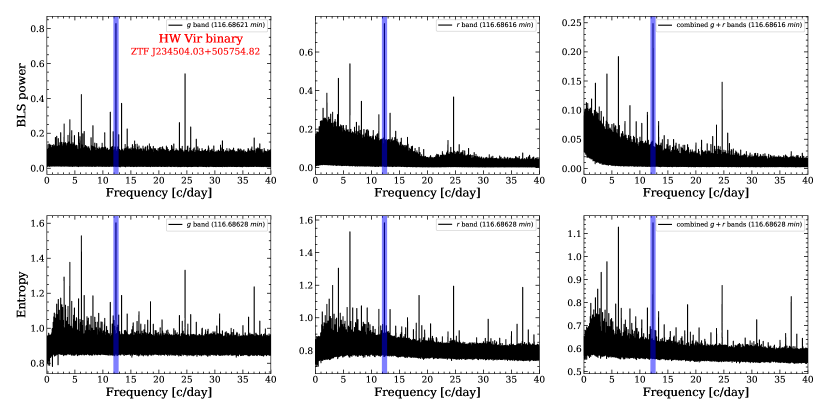
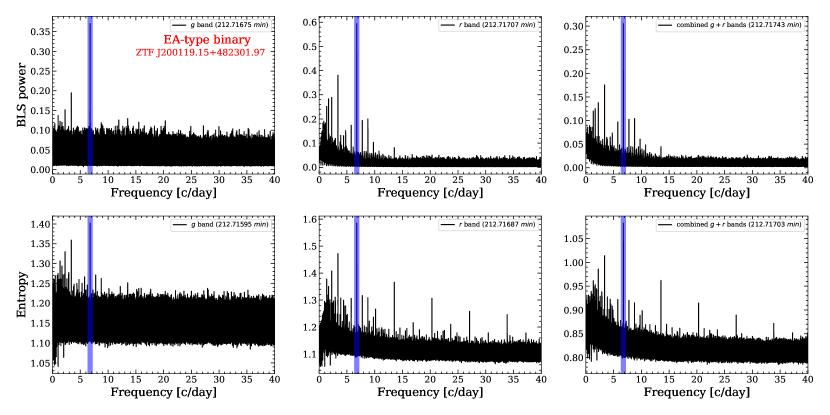
Figure 16: Examples of the variability types of light curve shapes caused by the binary eclipse effect in our binary sample. All panels show the frequency spectra of the BLS and CE corresponding to the above (Figure 4) variability types of the HW Vir binary and EA-type binary.

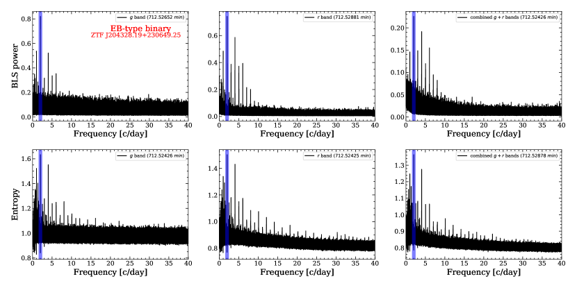
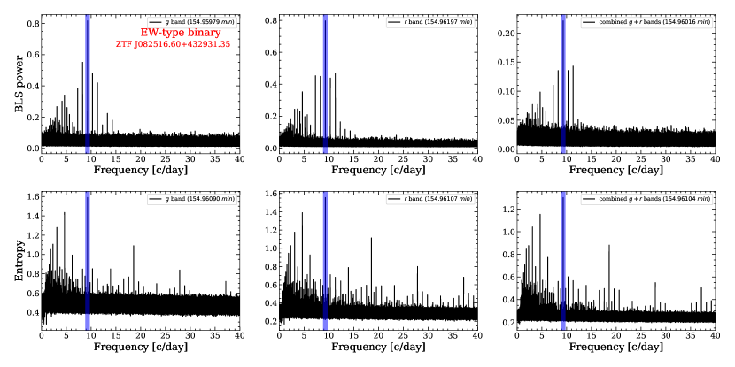
Figure 17: Examples of the variability types of light curve shapes caused by the binary eclipse effect in our binary sample. All panels show the frequency spectra of the BLS and CE corresponding to the above (Figure 4) variability types of the EB-type binary and EW-type binary.

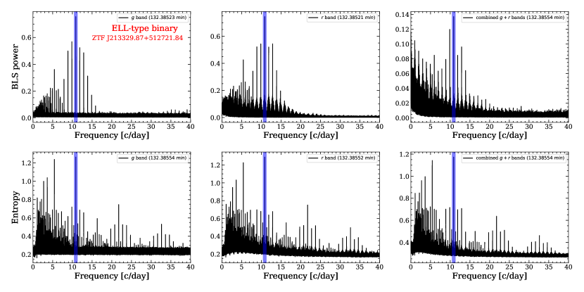
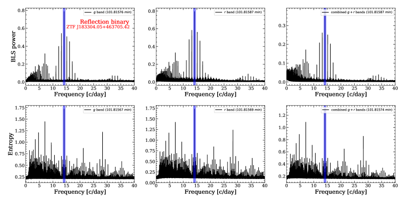
Figure 18: Examples of the variability types of light curve shapes caused by the binary eclipse effect in our binary sample. All panels show the frequency spectra of the BLS and CE corresponding to the above (Figure 4) variability types of the ELL-type binary and Reflection binary.

Appendix D Light curve-selected Targets

The phase ZTF ZTF g-band and r-band light curves of potential GW source candidates with an orbital period of less than 100 min in the binary sample. For further details on these light curves, please see Figures 19 and 20 .

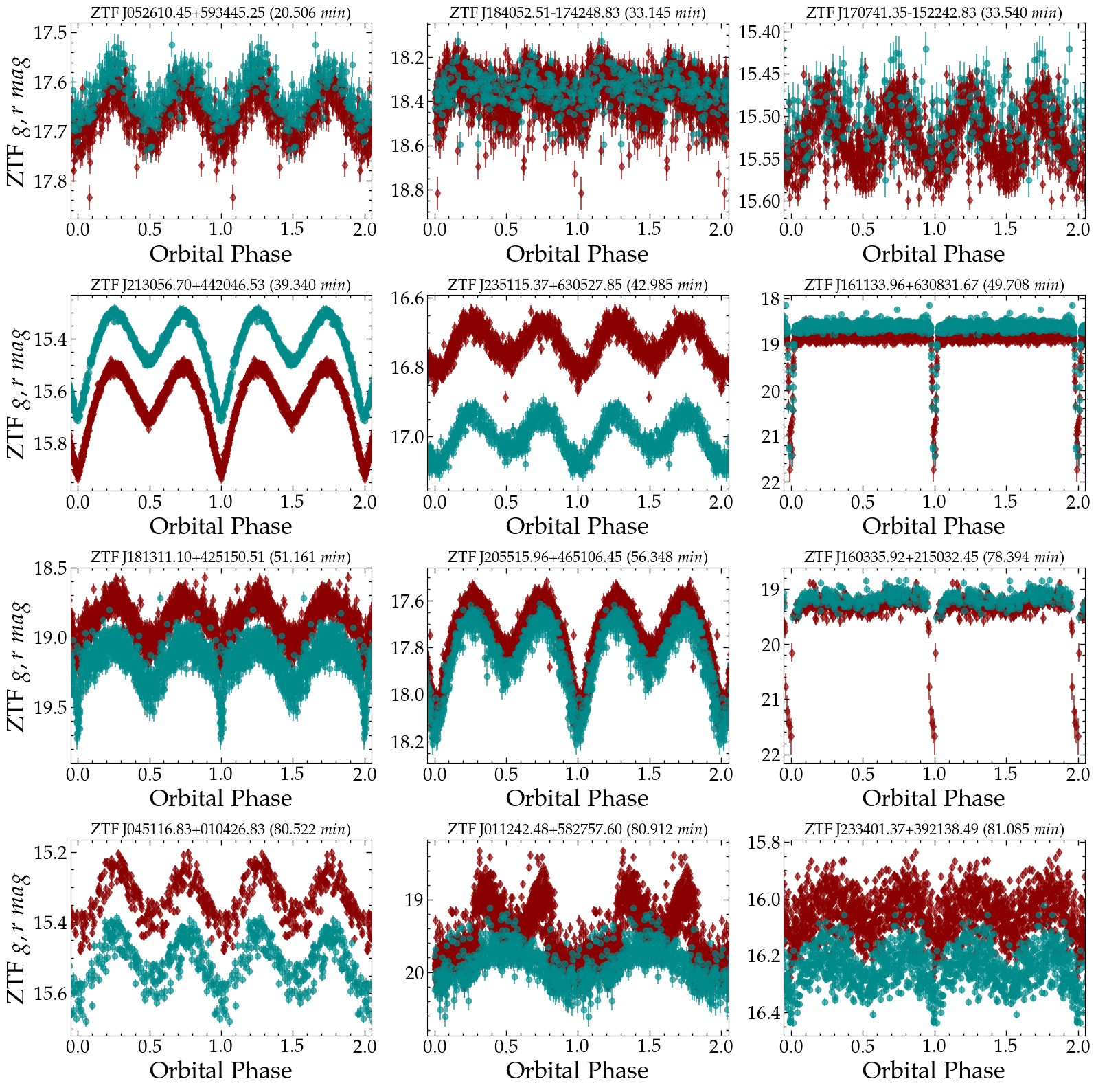
Figure 19: Phase-folded ZTF lightcurves of the potential GW candidates with an orbital period of less than 100 min, at GW amplitude and TianQin/LISA SNRs for these candidates described in Section 6.4.

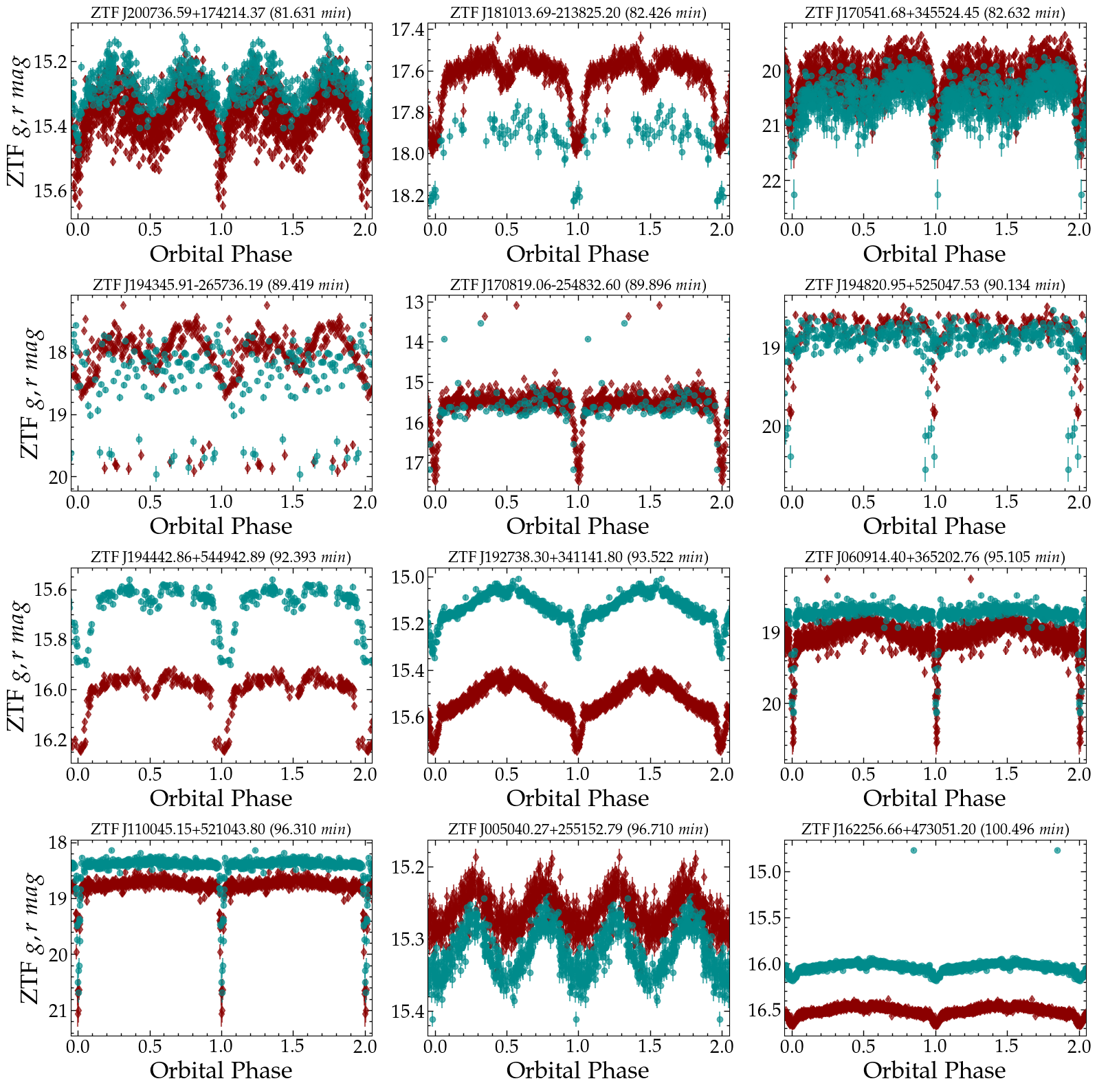
Figure 20: Phase-folded ZTF lightcurves of the potential GW candidates with an orbital period of less than 100 min, at GW amplitude and TianQin/LISA SNRs for these candidates described in Section 6.4.

References

- Ablimit (2022) Ablimit, I. 2022, MNRAS, 509, 6061, doi: 10.1093/mnras/stab3060
- Abrahams et al. (2020) Abrahams, E. S., Bloom, J. S., Mowlavi, N., et al. 2020, arXiv e-prints, arXiv:2011.12253. https://arxiv.org/abs/2011.12253
- Almeida et al. (2012) Almeida, L. A., Jablonski, F., Tello, J., & Rodrigues, C. V. 2012, MNRAS, 423, 478, doi: 10.1111/j.1365-2966.2012.20891.x
- Amaro-Seoane et al. (2017) Amaro-Seoane, P., Audley, H., Babak, S., et al. 2017, arXiv e-prints, arXiv:1702.00786. https://arxiv.org/abs/1702.00786
- Amaro-Seoane et al. (2022) Amaro-Seoane, P., Andrews, J., Arca Sedda, M., et al. 2022, arXiv e-prints, arXiv:2203.06016. https://arxiv.org/abs/2203.06016
- Amaro Seoane et al. (2022) Amaro Seoane, P., Arca Sedda, M., Babak, S., et al. 2022, General Relativity and Gravitation, 54, 3, doi: 10.1007/s10714-021-02889-x
- Astropy Collaboration et al. (2013) Astropy Collaboration, Robitaille, T. P., Tollerud, E. J., et al. 2013, A&A, 558, A33, doi: 10.1051/0004-6361/201322068
- Barlow et al. (2013) Barlow, B. N., Kilkenny, D., Drechsel, H., et al. 2013, MNRAS, 430, 22, doi: 10.1093/mnras/sts271
- Barlow et al. (2022) Barlow, B. N., Corcoran, K. A., Parker, I. M., et al. 2022, ApJ, 928, 20, doi: 10.3847/1538-4357/ac49f1
- Bellm et al. (2019) Bellm, E. C., Kulkarni, S. R., Graham, M. J., et al. 2019, PASP, 131, 018002, doi: 10.1088/1538-3873/aaecbe
- Boileau et al. (2021) Boileau, G., Lamberts, A., Christensen, N., Cornish, N. J., & Meyer, R. 2021, MNRAS, 508, 803, doi: 10.1093/mnras/stab2575
- Breedt et al. (2014) Breedt, E., Gänsicke, B. T., Drake, A. J., et al. 2014, MNRAS, 443, 3174, doi: 10.1093/mnras/stu1377
- Brown et al. (2016) Brown, W. R., Gianninas, A., Kilic, M., Kenyon, S. J., & Allende Prieto, C. 2016, ApJ, 818, 155, doi: 10.3847/0004-637X/818/2/155
- Brown et al. (2013) Brown, W. R., Kilic, M., Allende Prieto, C., Gianninas, A., & Kenyon, S. J. 2013, ApJ, 769, 66, doi: 10.1088/0004-637X/769/1/66
- Brown et al. (2010) Brown, W. R., Kilic, M., Allende Prieto, C., & Kenyon, S. J. 2010, ApJ, 723, 1072, doi: 10.1088/0004-637X/723/2/1072
- Brown et al. (2012) —. 2012, ApJ, 744, 142, doi: 10.1088/0004-637X/744/2/142
- Brown et al. (2020a) Brown, W. R., Kilic, M., Bédard, A., Kosakowski, A., & Bergeron, P. 2020a, ApJ, 892, L35, doi: 10.3847/2041-8213/ab8228
- Brown et al. (2011) Brown, W. R., Kilic, M., Hermes, J. J., et al. 2011, ApJ, 737, L23, doi: 10.1088/2041-8205/737/1/L23
- Brown et al. (2022) Brown, W. R., Kilic, M., Kosakowski, A., & Gianninas, A. 2022, ApJ, 933, 94, doi: 10.3847/1538-4357/ac72ac
- Brown et al. (2020b) Brown, W. R., Kilic, M., Kosakowski, A., et al. 2020b, ApJ, 889, 49, doi: 10.3847/1538-4357/ab63cd
- Burdge et al. (2019a) Burdge, K. B., Coughlin, M. W., Fuller, J., et al. 2019a, Nature, 571, 528, doi: 10.1038/s41586-019-1403-0
- Burdge et al. (2019b) Burdge, K. B., Fuller, J., Phinney, E. S., et al. 2019b, ApJ, 886, L12, doi: 10.3847/2041-8213/ab53e5
- Burdge et al. (2020a) Burdge, K. B., Coughlin, M. W., Fuller, J., et al. 2020a, ApJ, 905, L7, doi: 10.3847/2041-8213/abca91
- Burdge et al. (2020b) Burdge, K. B., Prince, T. A., Fuller, J., et al. 2020b, ApJ, 905, 32, doi: 10.3847/1538-4357/abc261
- Burdge et al. (2022) Burdge, K. B., El-Badry, K., Marsh, T. R., et al. 2022, arXiv e-prints, arXiv:2210.01809. https://arxiv.org/abs/2210.01809
- Chandra et al. (2021) Chandra, V., Hwang, H.-C., Zakamska, N. L., et al. 2021, ApJ, 921, 160, doi: 10.3847/1538-4357/ac2145
- Cheng et al. (2020) Cheng, S., Cummings, J. D., Ménard, B., & Toonen, S. 2020, ApJ, 891, 160, doi: 10.3847/1538-4357/ab733c
- Cornish & Larson (2003) Cornish, N. J., & Larson, S. L. 2003, Phys. Rev. D, 67, 103001, doi: 10.1103/PhysRevD.67.103001
- Coughlin et al. (2020) Coughlin, M. W., Burdge, K., Phinney, E. S., et al. 2020, MNRAS, 494, L91, doi: 10.1093/mnrasl/slaa044
- Culpan et al. (2022) Culpan, R., Geier, S., Reindl, N., et al. 2022, A&A, 662, A40, doi: 10.1051/0004-6361/202243337
- Deason et al. (2017) Deason, A. J., Belokurov, V., Erkal, D., Koposov, S. E., & Mackey, D. 2017, MNRAS, 467, 2636, doi: 10.1093/mnras/stx263
- Dekany et al. (2020) Dekany, R., Smith, R. M., Riddle, R., et al. 2020, PASP, 132, 038001, doi: 10.1088/1538-3873/ab4ca2
- Dimitrov & Kjurkchieva (2012) Dimitrov, D. P., & Kjurkchieva, D. P. 2012, New A, 17, 34, doi: 10.1016/j.newast.2011.06.005
- Duffy et al. (2021) Duffy, C., Ramsay, G., Steeghs, D., et al. 2021, MNRAS, 502, 4953, doi: 10.1093/mnras/stab389
- El-Badry et al. (2021a) El-Badry, K., Rix, H.-W., & Heintz, T. M. 2021a, MNRAS, 506, 2269, doi: 10.1093/mnras/stab323
- El-Badry et al. (2021b) El-Badry, K., Rix, H.-W., Quataert, E., Kupfer, T., & Shen, K. J. 2021b, MNRAS, 508, 4106, doi: 10.1093/mnras/stab2583
- El-Badry et al. (2021c) El-Badry, K., Quataert, E., Rix, H.-W., et al. 2021c, MNRAS, 505, 2051, doi: 10.1093/mnras/stab1318
- For et al. (2010) For, B. Q., Green, E. M., Fontaine, G., et al. 2010, ApJ, 708, 253, doi: 10.1088/0004-637X/708/1/253
- Geier et al. (2017) Geier, S., Østensen, R. H., Nemeth, P., et al. 2017, A&A, 600, A50, doi: 10.1051/0004-6361/201630135
- Geier et al. (2019) Geier, S., Raddi, R., Gentile Fusillo, N. P., & Marsh, T. R. 2019, A&A, 621, A38, doi: 10.1051/0004-6361/201834236
- Geier et al. (2011) Geier, S., Schaffenroth, V., Drechsel, H., et al. 2011, ApJ, 731, L22, doi: 10.1088/2041-8205/731/2/L22
- Geier et al. (2013) Geier, S., Marsh, T. R., Wang, B., et al. 2013, A&A, 554, A54, doi: 10.1051/0004-6361/201321395
- Gentile Fusillo et al. (2019) Gentile Fusillo, N. P., Tremblay, P.-E., Gänsicke, B. T., et al. 2019, MNRAS, 482, 4570, doi: 10.1093/mnras/sty3016
- Gentile Fusillo et al. (2021) Gentile Fusillo, N. P., Tremblay, P. E., Cukanovaite, E., et al. 2021, MNRAS, 508, 3877, doi: 10.1093/mnras/stab2672
- Gianninas et al. (2015) Gianninas, A., Kilic, M., Brown, W. R., Canton, P., & Kenyon, S. J. 2015, ApJ, 812, 167, doi: 10.1088/0004-637X/812/2/167
- Gokhale et al. (2007) Gokhale, V., Peng, X. M., & Frank, J. 2007, ApJ, 655, 1010, doi: 10.1086/510119
- Gong et al. (2021) Gong, Y., Luo, J., & Wang, B. 2021, Nature Astronomy, 5, 881, doi: 10.1038/s41550-021-01480-3
- Götberg et al. (2020) Götberg, Y., Korol, V., Lamberts, A., et al. 2020, ApJ, 904, 56, doi: 10.3847/1538-4357/abbda5
- Graham et al. (2013a) Graham, M. J., Drake, A. J., Djorgovski, S. G., Mahabal, A. A., & Donalek, C. 2013a, MNRAS, 434, 2629, doi: 10.1093/mnras/stt1206
- Graham et al. (2013b) Graham, M. J., Drake, A. J., Djorgovski, S. G., et al. 2013b, MNRAS, 434, 3423, doi: 10.1093/mnras/stt1264
- Graham et al. (2019) Graham, M. J., Kulkarni, S. R., Bellm, E. C., et al. 2019, PASP, 131, 078001, doi: 10.1088/1538-3873/ab006c
- Green et al. (2018) Green, M. J., Marsh, T. R., Steeghs, D. T. H., et al. 2018, MNRAS, 476, 1663, doi: 10.1093/mnras/sty299
- Green et al. (2020) Green, M. J., Marsh, T. R., Carter, P. J., et al. 2020, MNRAS, 496, 1243, doi: 10.1093/mnras/staa1509
- Guidry et al. (2021) Guidry, J. A., Vanderbosch, Z. P., Hermes, J. J., et al. 2021, ApJ, 912, 125, doi: 10.3847/1538-4357/abee68
- Guo et al. (2015) Guo, J., Zhao, J., Tziamtzis, A., et al. 2015, MNRAS, 454, 2787, doi: 10.1093/mnras/stv2104
- Harris et al. (2020) Harris, C. R., Millman, K. J., van der Walt, S. J., et al. 2020, Nature, 585, 357, doi: 10.1038/s41586-020-2649-2
- Heber (2016) Heber, U. 2016, PASP, 128, 082001, doi: 10.1088/1538-3873/128/966/082001
- Hernandez et al. (2021) Hernandez, M. S., Schreiber, M. R., Parsons, S. G., et al. 2021, MNRAS, 501, 1677, doi: 10.1093/mnras/staa3815
- Hernandez et al. (2022) —. 2022, MNRAS, 512, 1843, doi: 10.1093/mnras/stac604
- Hillman et al. (2020) Hillman, Y., Shara, M. M., Prialnik, D., & Kovetz, A. 2020, Nature Astronomy, 4, 886, doi: 10.1038/s41550-020-1062-y
- Huang et al. (2020) Huang, S.-J., Hu, Y.-M., Korol, V., et al. 2020, Phys. Rev. D, 102, 063021, doi: 10.1103/PhysRevD.102.063021
- Hunter (2007) Hunter, J. D. 2007, Computing in Science and Engineering, 9, 90, doi: 10.1109/MCSE.2007.55
- Inight et al. (2021) Inight, K., Gänsicke, B. T., Breedt, E., et al. 2021, MNRAS, 504, 2420, doi: 10.1093/mnras/stab753
- IRSA (2022) IRSA. 2022, Time Series Tool, IPAC, doi: 10.26131/IRSA538. https://catcopy.ipac.caltech.edu/dois/doi.php?id=10.26131/IRSA538
- Jiang et al. (2013) Jiang, B., Luo, A., Zhao, Y., & Wei, P. 2013, MNRAS, 430, 986, doi: 10.1093/mnras/sts665
- Kalomeni et al. (2016) Kalomeni, B., Nelson, L., Rappaport, S., et al. 2016, ApJ, 833, 83, doi: 10.3847/1538-4357/833/1/83
- Kao et al. (2016) Kao, W., Kaplan, D. L., Prince, T. A., et al. 2016, MNRAS, 461, 2747, doi: 10.1093/mnras/stw1434
- Katz et al. (2021) Katz, M. L., Cooper, O. R., Coughlin, M. W., et al. 2021, MNRAS, 503, 2665, doi: 10.1093/mnras/stab504
- Keller et al. (2022) Keller, P. M., Breedt, E., Hodgkin, S., et al. 2022, MNRAS, 509, 4171, doi: 10.1093/mnras/stab3293
- Kilic et al. (2011) Kilic, M., Brown, W. R., Allende Prieto, C., et al. 2011, ApJ, 727, 3, doi: 10.1088/0004-637X/727/1/3
- Kilic et al. (2012) —. 2012, ApJ, 751, 141, doi: 10.1088/0004-637X/751/2/141
- Kilic et al. (2021) Kilic, M., Brown, W. R., Bédard, A., & Kosakowski, A. 2021, ApJ, 918, L14, doi: 10.3847/2041-8213/ac1e2b
- Kilic et al. (2014) Kilic, M., Brown, W. R., Gianninas, A., et al. 2014, MNRAS, 444, L1, doi: 10.1093/mnrasl/slu093
- Kjurkchieva et al. (2015) Kjurkchieva, D., Khruzina, T., Dimitrov, D., et al. 2015, A&A, 584, A40, doi: 10.1051/0004-6361/201526102
- Knigge et al. (2011) Knigge, C., Baraffe, I., & Patterson, J. 2011, ApJS, 194, 28, doi: 10.1088/0067-0049/194/2/28
- Kolbin & Borisov (2020) Kolbin, A. I., & Borisov, N. V. 2020, Astronomy Letters, 46, 812, doi: 10.1134/S1063773720120026
- Kolbin et al. (2022) Kolbin, A. I., Borisov, N. V., Serebriakova, N. A., et al. 2022, MNRAS, 511, 20, doi: 10.1093/mnras/stab3676
- Korol et al. (2017) Korol, V., Rossi, E. M., Groot, P. J., et al. 2017, MNRAS, 470, 1894, doi: 10.1093/mnras/stx1285
- Kosakowski et al. (2022) Kosakowski, A., Kilic, M., Brown, W. R., Bergeron, P., & Kupfer, T. 2022, MNRAS, 516, 720, doi: 10.1093/mnras/stac1146
- Kosakowski et al. (2020) Kosakowski, A., Kilic, M., Brown, W. R., & Gianninas, A. 2020, ApJ, 894, 53, doi: 10.3847/1538-4357/ab8300
- Kovács et al. (2002) Kovács, G., Zucker, S., & Mazeh, T. 2002, A&A, 391, 369, doi: 10.1051/0004-6361:20020802
- Kramer et al. (2020) Kramer, M., Schneider, F. R. N., Ohlmann, S. T., et al. 2020, A&A, 642, A97, doi: 10.1051/0004-6361/202038702
- Kruckow et al. (2021) Kruckow, M. U., Neunteufel, P. G., Di Stefano, R., Gao, Y., & Kobayashi, C. 2021, ApJ, 920, 86, doi: 10.3847/1538-4357/ac13ac
- Kupfer et al. (2018) Kupfer, T., Korol, V., Shah, S., et al. 2018, MNRAS, 480, 302, doi: 10.1093/mnras/sty1545
- Kupfer et al. (2019) Kupfer, T., Bauer, E. B., Burdge, K. B., et al. 2019, ApJ, 878, L35, doi: 10.3847/2041-8213/ab263c
- Kupfer et al. (2020a) Kupfer, T., Bauer, E. B., Marsh, T. R., et al. 2020a, ApJ, 891, 45, doi: 10.3847/1538-4357/ab72ff
- Kupfer et al. (2020b) Kupfer, T., Bauer, E. B., Burdge, K. B., et al. 2020b, ApJ, 898, L25, doi: 10.3847/2041-8213/aba3c2
- Kupfer et al. (2021) Kupfer, T., Prince, T. A., van Roestel, J., et al. 2021, MNRAS, 505, 1254, doi: 10.1093/mnras/stab1344
- Kupfer et al. (2022) Kupfer, T., Bauer, E. B., van Roestel, J., et al. 2022, ApJ, 925, L12, doi: 10.3847/2041-8213/ac48f1
- Lagos et al. (2022) Lagos, F., Schreiber, M. R., Parsons, S. G., et al. 2022, MNRAS, 512, 2625, doi: 10.1093/mnras/stac673
- Lagos et al. (2020) —. 2020, MNRAS, 494, 915, doi: 10.1093/mnras/staa747
- Lei et al. (2020) Lei, Z., Zhao, J., Németh, P., & Zhao, G. 2020, ApJ, 889, 117, doi: 10.3847/1538-4357/ab660a
- Leroy (2012) Leroy, B. 2012, A&A, 545, A50, doi: 10.1051/0004-6361/201219076
- Li et al. (2022) Li, J., Onken, C. A., Wolf, C., et al. 2022, MNRAS, 515, 3370, doi: 10.1093/mnras/stac1768
- Li et al. (2019) Li, Z., Chen, X., Chen, H.-L., & Han, Z. 2019, ApJ, 871, 148, doi: 10.3847/1538-4357/aaf9a1
- Liang et al. (2022) Liang, Z.-C., Hu, Y.-M., Jiang, Y., et al. 2022, Phys. Rev. D, 105, 022001, doi: 10.1103/PhysRevD.105.022001
- Lindegren et al. (2018) Lindegren, L., Hernández, J., Bombrun, A., et al. 2018, A&A, 616, A2, doi: 10.1051/0004-6361/201832727
- Lindegren et al. (2021) Lindegren, L., Klioner, S. A., Hernández, J., et al. 2021, A&A, 649, A2, doi: 10.1051/0004-6361/202039709
- Liu & Wang (2020) Liu, D., & Wang, B. 2020, MNRAS, 494, 3422, doi: 10.1093/mnras/staa963
- Liu et al. (2018) Liu, D., Wang, B., & Han, Z. 2018, MNRAS, 473, 5352, doi: 10.1093/mnras/stx2756
- Lomb (1976) Lomb, N. R. 1976, Ap&SS, 39, 447, doi: 10.1007/BF00648343
- Lu et al. (2022) Lu, Y., Li, E.-K., Hu, Y.-M., Zhang, J.-d., & Mei, J. 2022, arXiv e-prints, arXiv:2205.02384. https://arxiv.org/abs/2205.02384
- Luo et al. (2016) Luo, J., Chen, L.-S., Duan, H.-Z., et al. 2016, Classical and Quantum Gravity, 33, 035010, doi: 10.1088/0264-9381/33/3/035010
- Masci et al. (2019) Masci, F. J., Laher, R. R., Rusholme, B., et al. 2019, PASP, 131, 018003, doi: 10.1088/1538-3873/aae8ac
- Maselli et al. (2020) Maselli, A., Marassi, S., & Branchesi, M. 2020, A&A, 635, A120, doi: 10.1051/0004-6361/201936848
- McKinney (2010) McKinney, W. 2010, in Proceedings of the 9th Python in Science Conference, ed. S. van der Walt & J. Millman
- McWhirter & Lam (2022) McWhirter, P. R., & Lam, M. C. 2022, MNRAS, 511, 4971, doi: 10.1093/mnras/stac291
- Mowlavi et al. (2021) Mowlavi, N., Rimoldini, L., Evans, D. W., et al. 2021, A&A, 648, A44, doi: 10.1051/0004-6361/202039450
- Nelemans et al. (2001a) Nelemans, G., Portegies Zwart, S. F., Verbunt, F., & Yungelson, L. R. 2001a, A&A, 368, 939, doi: 10.1051/0004-6361:20010049
- Nelemans et al. (2001b) Nelemans, G., Yungelson, L. R., Portegies Zwart, S. F., & Verbunt, F. 2001b, A&A, 365, 491, doi: 10.1051/0004-6361:20000147
- Norton et al. (1999) Norton, A. J., Beardmore, A. P., Allan, A., & Hellier, C. 1999, A&A, 347, 203. https://arxiv.org/abs/astro-ph/9811310
- Ofek et al. (2020) Ofek, E. O., Soumagnac, M., Nir, G., et al. 2020, MNRAS, 499, 5782, doi: 10.1093/mnras/staa2814
- Panahi & Zucker (2021) Panahi, A., & Zucker, S. 2021, PASP, 133, 024502, doi: 10.1088/1538-3873/abd9ab
- Parsons et al. (2016) Parsons, S. G., Rebassa-Mansergas, A., Schreiber, M. R., et al. 2016, MNRAS, 463, 2125, doi: 10.1093/mnras/stw2143
- Pelisoli et al. (2019) Pelisoli, I., Bell, K. J., Kepler, S. O., & Koester, D. 2019, MNRAS, 482, 3831, doi: 10.1093/mnras/sty2979
- Pelisoli & Vos (2019) Pelisoli, I., & Vos, J. 2019, MNRAS, 488, 2892, doi: 10.1093/mnras/stz1876
- Pelisoli et al. (2021) Pelisoli, I., Neunteufel, P., Geier, S., et al. 2021, Nature Astronomy, 5, 1052, doi: 10.1038/s41550-021-01413-0
- Perez & Granger (2007) Perez, F., & Granger, B. E. 2007, Computing in Science and Engineering, 9, 21, doi: 10.1109/MCSE.2007.53
- Pichardo Marcano et al. (2021a) Pichardo Marcano, M., Rivera Sandoval, L. E., Maccarone, T. J., & Scaringi, S. 2021a, MNRAS, 508, 3275, doi: 10.1093/mnras/stab2685
- Pichardo Marcano et al. (2021b) —. 2021b, MNRAS, 508, 3275, doi: 10.1093/mnras/stab2685
- Postnov & Yungelson (2014) Postnov, K. A., & Yungelson, L. R. 2014, Living Reviews in Relativity, 17, 3, doi: 10.12942/lrr-2014-3
- Ramsay et al. (2018) Ramsay, G., Green, M. J., Marsh, T. R., et al. 2018, A&A, 620, A141, doi: 10.1051/0004-6361/201834261
- Rebassa-Mansergas et al. (2019) Rebassa-Mansergas, A., Toonen, S., Korol, V., & Torres, S. 2019, MNRAS, 482, 3656, doi: 10.1093/mnras/sty2965
- Rebassa-Mansergas et al. (2017) Rebassa-Mansergas, A., Ren, J. J., Irawati, P., et al. 2017, MNRAS, 472, 4193, doi: 10.1093/mnras/stx2259
- Rebassa-Mansergas et al. (2021) Rebassa-Mansergas, A., Solano, E., Jiménez-Esteban, F. M., et al. 2021, MNRAS, 506, 5201, doi: 10.1093/mnras/stab2039
- Ren et al. (2020) Ren, J. J., Raddi, R., Rebassa-Mansergas, A., et al. 2020, ApJ, 905, 38, doi: 10.3847/1538-4357/abc017
- Rivera Sandoval et al. (2022) Rivera Sandoval, L. E., Heinke, C. O., Hameury, J. M., et al. 2022, ApJ, 926, 10, doi: 10.3847/1538-4357/ac3fb7
- Robson et al. (2019) Robson, T., Cornish, N. J., & Liu, C. 2019, Classical and Quantum Gravity, 36, 105011, doi: 10.1088/1361-6382/ab1101
- Sale et al. (2020) Sale, O., Bogensberger, D., Clarke, F., & Lynas-Gray, A. E. 2020, MNRAS, 499, 3071, doi: 10.1093/mnras/staa3013
- Scargle (1982) Scargle, J. D. 1982, ApJ, 263, 835, doi: 10.1086/160554
- Schreiber et al. (2021) Schreiber, M. R., Belloni, D., Gänsicke, B. T., Parsons, S. G., & Zorotovic, M. 2021, Nature Astronomy, 5, 648, doi: 10.1038/s41550-021-01346-8
- Schreiber et al. (2022) Schreiber, M. R., Belloni, D., Zorotovic, M., et al. 2022, MNRAS, doi: 10.1093/mnras/stac1076
- Shahaf et al. (2022) Shahaf, S., Zackay, B., Mazeh, T., Faigler, S., & Ivashtenko, O. 2022, MNRAS, doi: 10.1093/mnras/stac960
- Shen et al. (2018) Shen, K. J., Boubert, D., Gänsicke, B. T., et al. 2018, ApJ, 865, 15, doi: 10.3847/1538-4357/aad55b
- Szkody et al. (2020) Szkody, P., Dicenzo, B., Ho, A. Y. Q., et al. 2020, AJ, 159, 198, doi: 10.3847/1538-3881/ab7cce
- Szkody et al. (2021) Szkody, P., Olde Loohuis, C., Koplitz, B., et al. 2021, AJ, 162, 94, doi: 10.3847/1538-3881/ac0efb
- Takata et al. (2022) Takata, J., Wang, X. F., Kong, A. K. H., et al. 2022, ApJ, 936, 134, doi: 10.3847/1538-4357/ac8100
- Toonen et al. (2012) Toonen, S., Nelemans, G., & Portegies Zwart, S. 2012, A&A, 546, A70, doi: 10.1051/0004-6361/201218966
- Torres et al. (2022) Torres, S., Canals, P., Jiménez-Esteban, F. M., Rebassa-Mansergas, A., & Solano, E. 2022, MNRAS, 511, 5462, doi: 10.1093/mnras/stac374
- van der Walt et al. (2011) van der Walt, S., Colbert, S. C., & Varoquaux, G. 2011, Computing in Science and Engineering, 13, 22, doi: 10.1109/MCSE.2011.37
- van Roestel et al. (2017) van Roestel, J., Groot, P. J., Levitan, D., et al. 2017, MNRAS, 468, 3109, doi: 10.1093/mnras/stx625
- van Roestel et al. (2018) van Roestel, J., Kupfer, T., Ruiz-Carmona, R., et al. 2018, MNRAS, 475, 2560, doi: 10.1093/mnras/stx3291
- van Roestel et al. (2021a) van Roestel, J., Kupfer, T., Green, M. J., et al. 2021a, MNRAS, doi: 10.1093/mnras/stab2421
- van Roestel et al. (2021b) van Roestel, J., Creter, L., Kupfer, T., et al. 2021b, AJ, 162, 113, doi: 10.3847/1538-3881/ac0622
- van Roestel et al. (2021c) —. 2021c, AJ, 162, 113, doi: 10.3847/1538-3881/ac0622
- VanderPlas (2018) VanderPlas, J. T. 2018, ApJS, 236, 16, doi: 10.3847/1538-4365/aab766
- Virtanen et al. (2020) Virtanen, P., Gommers, R., Oliphant, T. E., et al. 2020, Nature Methods, 17, 261, doi: 10.1038/s41592-019-0686-2
- Wang et al. (2022a) Wang, B., Liu, D., & Chen, H. 2022a, MNRAS, 510, 6011, doi: 10.1093/mnras/stac114
- Wang et al. (2021) Wang, K., Kupfer, T., & Barlow, B. N. 2021, arXiv e-prints, arXiv:2112.12868. https://arxiv.org/abs/2112.12868
- Wang et al. (2022b) Wang, K., Németh, P., Luo, Y., et al. 2022b, ApJ, 936, 5, doi: 10.3847/1538-4357/ac847c
- Wang et al. (2020) Wang, K., Zhang, X., & Dai, M. 2020, ApJ, 888, 49, doi: 10.3847/1538-4357/ab584c
- Wevers et al. (2016) Wevers, T., Torres, M. A. P., Jonker, P. G., et al. 2016, MNRAS, 462, L106, doi: 10.1093/mnrasl/slw141
- Wong & Bildsten (2021) Wong, T. L. S., & Bildsten, L. 2021, ApJ, 923, 125, doi: 10.3847/1538-4357/ac2b2a
- Yu et al. (2019) Yu, Y.-W., Chen, A., & Wang, B. 2019, ApJ, 870, L23, doi: 10.3847/2041-8213/aaf960