Linear power corrections to single top production processes at the LHC

Abstract

We discuss the linear power corrections to the electroweak production of top quarks at the LHC using renormalon calculus. We show how such non-perturbative corrections can be obtained using the Low-Burnett-Kroll theorem, which provides the first subleading term to the expansion of the real-emission amplitudes around the soft limit. We demonstrate that there are no linear power corrections to the total cross sections of arbitrary processes of a single top production type provided that these cross sections are expressed in terms of a short-distance top quark mass. We also derive a universal formula for the linear power corrections to generic observables that involve the top-quark momentum.

1 Introduction

High rates and clean signatures of top quark production processes at the LHC have ushered the era of high-precision exploration of top quark properties. Such studies can be performed in processes where top quarks and anti-top quarks are produced in pairs via strong interactions, and also in processes where single top quarks are produced by flavor-changing electroweak charged currents.

Among many interesting quantities that one can study in such processes, the top quark mass plays a particularly important role. Experimentally, the top quark mass is already measured with very high precision and further improvements are expected at the high-luminosity LHC. Theoretically, there is a debate about non-perturbative effects that affect all existing top quark measurements and require better understanding.

In the past, many of these discussions were framed as a dispute about the type of mass that is best extracted from a particular measurement. It was sometimes argued that short-distance mass renormalisation schemes, for example the $\overline{\text{MS}}$ scheme, are preferable over the pole-mass scheme because the pole mass is affected by infrared renormalons Bigi:1994em ; Beneke:1994sw . Studies of the apparent convergence of the perturbative expansion in different mass schemes have also been performed to support these arguments Langenfeld:2009wd ; Dowling:2013baa ; Makela:2023wbk .

However, it is far from obvious that the top quark mass renormalon is the only renormalon that affects top quark production, in spite of being the one that has attracted most attention. Moreover, since no first-principles understanding of the non-perturbative effects in hadron collider processes currently exists, ultra-precise determinations of many fundamental parameters at the LHC, including the top quark mass, remain obscure.

A possible step towards a better understanding of the non-perturbative contributions to relevant LHC processes, including heavy quark production, is to study power corrections using renormalon calculus. This technique works under the assumption that the renormalon contributions are dominated by the large value of $b_{0}$, the coefficient of the leading term of the QCD $\beta$-function. More specifically, one starts with a model theory with a large negative value of massless quark species $n_{f}$, and considers only the dominant terms in the perturbative expansion, proportional to powers of $\alpha_{s}n_{f}$. In this limit the coefficient of the leading term of the beta function equals $b_{0,n_{f}}=-4T_{F}n_{f}/(12\pi)$; it is positive for negative $n_{f}$, so that the model theory is asymptotically free. At the end of the calculation one replaces $b_{0,n_{f}}$ with $b_{0}$-value in QCD, $b_{0}=(11C_{A}-4T_{F}n_{f})/(12\pi)$.

It turns out that the results in the large-$b_{0}$ approximation can be easily obtained from calculations in QCD where the gluon carries a small mass $\lambda$. It can be shown that, if an observable is linearly sensitive to $\lambda$, there is a renormalon in the perturbative expansion of this observable associated with a power correction of order $\Lambda_{\rm QCD}$. This procedure is well known, and it has been reviewed in ref. Beneke:1998ui , where many applications are also discussed. A complete account of how these calculations are carried out, also including the contribution of non-inclusive real corrections, is given in Appendix B of ref. FerrarioRavasio:2018ubr .

Unfortunately, the application of the renormalon calculus is currently limited to processes where no gluons appear in the Feynman diagrams that contribute at the leading order. This feature prevents us from applying the renormalon analysis to studying non-perturbative effects in the top quark pair production process. However, the non-perturbative contributions to the $t$-channel single top production process can be analysed using the renormalon calculus, since at the leading order this process is a flavor-changing quark-quark scattering mediated by the exchange of a $W$-boson.

We will show that such non-perturbative contributions can be determined for a class of processes $pp\to t+X+q$, where $X$ is an arbitrary collection of colourless particles, using the so-called Low-Burnett-Kroll (LBK) theorem Low:1958sn ; Burnett:1967km , which allows one to obtain the first sub-leading contribution to the expansion of the scattering amplitude for soft radiation. Following the logic of the LBK theorem, we will also be able to compute the renormalon structure of the virtual corrections to the same generic process.

The rest of the paper is organised as follows. In the next section we discuss the real emission contribution to the process $pp\to t+q+g+X$ and explain how the ${\cal O}(\lambda)$ corrections to the fully-differential partonic cross section can be computed using the Low-Burnett-Kroll theorem. In Section 3 we generalise this result to the computation of the virtual corrections. In Section 4 we combine the virtual corrections with various renormalisation contributions. In Section 5 we explain how to compute the change in the cross section due to a top quark mass redefinition. In Section 6 we combine the various contributions and show that the linear ${\cal O}(\Lambda_{\rm QCD})$ power corrections cancel in the total cross section provided that a short-distance top-quark mass scheme is used. In Section 7 we illustrate an alternative way to compute the effect of the self-energy insertions in the external top line, that allows one to perform the calculation directly in any short-distance mass scheme. In Section 8 we describe the computation of the ${\cal O}(\Lambda_{\rm QCD})$ corrections to observables that depend on the top quark momentum; at variance with the total cross section, we find that there are linear power corrections to such observables. We present our conclusions in Section 9. In Appendix A we provide results for real and virtual integrals that we have used in the calculation, while in Appendix B we show how to reproduce the well-known result Bigi:1994em ; Beneke:1994bc on the absence of the ${\cal O}(\Lambda_{\rm QCD})$ corrections to semileptonic decays of a heavy quark using our technique.

2 Real emission contribution to single top production and the Low-Burnett-Kroll theorem

We consider the process of $t$-channel single top production in association with a colourless system $X$

$$u(p_{u})+b(p_{b})\to d(p_{d})+t(p_{t})+X(p_{X}),$$ (1)

and write the kinematics for the real correction to this process due to the emission of a massive gluon as follows

$$u(p_{u})+b(p_{b})\to d(q_{d})+t(q_{t})+X(p_{X})+g(k).$$ (2)

We note that we have used different notations for the four-momenta of the top quark and the down quark in the two cases. This is done for future convenience since, as we will see, these momenta will absorb the recoil due to the emitted soft gluon.

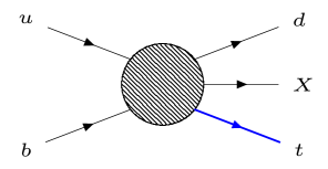
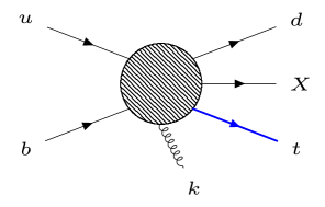
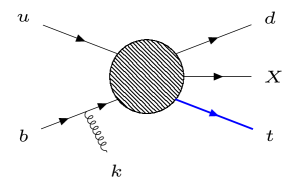
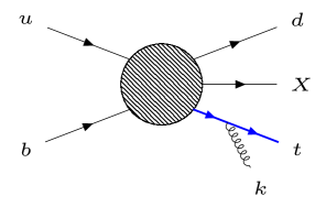
Figure 1: Leading order and the relevant real emission contributions to a single top production process. The blob in the center represents the function ${\bf N}$. We emphasise that there is no colour transfer from the light quark line to the heavy quark line, see text for details.

The gluon can be emitted from the “light” quark line (i.e. the fermion line going from the up to the down quark) or from the “heavy” quark line (i.e. the one from the bottom quark to the top quark). However, since the process is mediated by an exchange of a colourless $W$-boson, the two contributions do not interfere because of colour conservation. As explained in ref. Caola:2021kzt , emissions off the light-quark line cannot produce linear power corrections; for this reason we do not discuss them further and focus instead on the emissions off the heavy quark line.

It is also explained in ref. Caola:2021kzt that one can only obtain ${\cal O}(\lambda)$ contributions to the cross section of the process eq. (2) if the gluon $g(k)$ is soft. However, since the leading term in the soft expansion corresponds to ${\cal O}(\lambda^{0})$, the first sub-leading term in the soft expansion is required. Such term can be obtained in a process-independent way using the LBK theorem Low:1958sn ; Burnett:1967km , as we now explain.

We write the amplitude extracting the strong coupling constant, the colour factor and the gluon polarisation vector. It reads

$${\cal A}_{\rm real}=g_{s}T^{a}_{ij}\epsilon_{\mu}{\cal M}^{\mu},$$ (3)

where $a,i,j$ are the gluon, top-quark and $b$-quark colour indices and $\epsilon$ is the gluon polarisation vector. The reduced amplitude ${\cal M}^{\mu}$ reads

$$\begin{split}\mathcal{M}^{\mu}&=\bar{u}(q_{t})\gamma^{\mu}\frac{{\not{q}}_{t}+{\not{k}}+m_{t}}{d_{t}}{\bf N}(q_{t}+k,p_{b},q_{d},...)u(p_{b})\\ &+\bar{u}(q_{t}){\bf N}(q_{t},p_{b}-k,q_{d},...)\frac{{\not{p}}_{b}-{\not{k}}}{d_{b}}\gamma^{\mu}u(p_{b})+{\cal M}^{\mu}_{\rm reg}(q_{t},p_{b},q_{d},..|k),\end{split}$$ (4)

where $d_{t}=(q_{t}+k)^{2}-m_{t}^{2}=2q_{t}k+\lambda^{2}$ and $d_{b}=(p_{b}-k)^{2}=-2p_{b}k+\lambda^{2}$. The three terms on the right-hand side of eq. (4) describe contributions where a gluon is emitted off an external top-quark line, an external $b$-quark line and, finally, off any internal part of the “heavy” line of the process, respectively. They are illustrated in Fig. 1. In the soft $k\sim\lambda\to 0$ limit, the first two terms in eq. (4) scale as $1/\lambda$ whereas the third term scales as $\lambda^{0}$. Hence, to compute the amplitude through sub-leading terms in the soft expansion, ${\cal M}^{\mu}_{\rm reg}(q_{t},p_{b},q_{d},..|k)$ is required.

The matrix function ${\bf N}$, which can be understood as a Green’s function of a Born-like process eq. (1) with amputated $t$ and $b$ lines, can be used to write the amplitude for the elastic no-emission process $u(p_{u})+b(p_{b})\to d(p_{d})+t(p_{t})+X(p_{X})$

$${\cal A}_{0}=\delta_{ij}\;\bar{u}(p_{t}){\bf N}(p_{t},p_{b},p_{d},..)u(p_{b}).$$ (5)

We note that we always assume that the energy-momentum conservation condition has been used to express the function ${\bf N}$ in eqs. (4, 5) through a unique set of momenta.

In general, diagrams where gluons are only emitted from the external $t$ and $b$ legs are not gauge invariant on their own; this fact can be used to determine the amplitude ${\cal M}^{\mu}_{\rm reg}(q_{t},p_{b},q_{d},..|k)$ Low:1958sn ; Burnett:1967km . To this end, we compute the scalar product of ${\cal M}^{\mu}$ with $k_{\mu}$ and demand that the result vanishes, as required by current conservation. We then find

$$0=\bar{u}_{t}{\bf N}(q_{t}+k,p_{b},q_{d},...)u_{b}-\bar{u}_{t}{\bf N}(q_{t},p_{b}-k,q_{d},...)u_{b}+k_{\mu}{\cal M}^{\mu}_{\rm reg}(q_{t},p_{b},q_{d},\dots|k),$$ (6)

where, for ease of notation, we do not display the arguments of the external spinors, i.e. $\bar{u}_{t}(q_{t})\Rightarrow\bar{u}_{t}$ and $u_{b}(p_{b})\Rightarrow u_{b}$. We will employ this notation through the end of this section.

We solve eq. (6) to zeroth order in the gluon momentum $k$ by expanding the function ${\bf N}$ and the function ${\cal M}^{\mu}_{\rm reg}$ in Taylor series in $k$. Neglecting terms of order $k^{2}$, we find

$$0=k^{\mu}\bar{u}_{t}\left[\frac{\partial{\bf N}(q_{t},p_{b},q_{d},...)}{\partial q_{t}^{\mu}}+\frac{\partial{\bf N}(q_{t},p_{b},q_{d},...)}{\partial p_{b}^{\mu}}\right]u_{b}+k_{\mu}{\cal M}^{\mu}_{\rm ext}(q_{t},p_{b},q_{d},\dots|k=0).$$ (7)

This equation should hold for any $k$; therefore

$${\cal M}^{\mu}_{\rm ext}(q_{t},p_{b},q_{d},...|k=0)=-\bar{u}_{t}\left[\frac{\partial{\bf N}(q_{t},p_{b},q_{d},...)}{\partial q_{t,\mu}}+\frac{\partial{\bf N}(q_{t},p_{b},q_{d},...)}{\partial p_{b,\mu}}\right]u_{b}.$$ (8)

To proceed further, we simplify the expressions for diagrams where the gluon is emitted off the external lines. We write

$$\bar{u}_{t}\gamma^{\mu}\frac{{\not{q}}_{t}+{\not{k}}+m_{t}}{d_{t}}=\bar{u}_{t}\frac{2q_{t}^{\mu}+k^{\mu}+\sigma^{\mu\nu}k_{\nu}}{d_{t}}=\bar{u}_{t}\left[J_{t}^{\mu}+{\bf S}_{t}^{\mu}\right],$$ (9)

where $\sigma^{\mu\nu}=\frac{1}{2}[\gamma^{\mu},\gamma^{\nu}]$ and we introduced spin-independent and spin-dependent currents

$$J_{t}^{\mu}=\frac{2q_{t}+k^{\mu}}{d_{t}},\;\;\;\;{\bf S}_{t}^{\mu}=\frac{\sigma^{\mu\nu}k_{\nu}}{d_{t}},$$ (10)

which describe the gluon emission off the top quark. Similarly,

$$\frac{{\not{p}}_{b}-{\not{k}}}{d_{b}}\gamma^{\mu}u_{b}=\frac{2p_{b}^{\mu}-k^{\mu}+\sigma^{\mu\nu}k_{\nu}}{d_{b}}u_{b}=\left[J_{b}^{\mu}+{\bf S}_{b}^{\mu}\right]u_{b},$$ (11)

where

$$J_{b}^{\mu}=\frac{2p_{b}^{\mu}-k^{\mu}}{d_{b}},\;\;\;\;{\bf S}_{b}^{\mu}=\frac{\sigma^{\mu\nu}k_{\nu}}{d_{b}}.$$ (12)

We can use these results to write the amplitude for a single gluon emission through the first sub-leading terms in the soft expansion. We find

$$\begin{split}{\cal M}^{\mu}&=J_{t}^{\mu}\bar{u}_{t}{\bf N}(q_{t}+k,p_{b},q_{d},..)u_{b}+J_{b}^{\mu}\bar{u}_{t}{\bf N}(q_{t},p_{b}-k,q_{d},..)u_{b}\\ &+\bar{u}_{t}\left[{\bf S}_{t}^{\mu}{\bf N}(q_{t},p_{b},q_{d},..)+{\bf N}(q_{t},p_{b},q_{d},..){\bf S}_{b}^{\mu}\right]u_{b}\\ &-\bar{u}_{t}\left[\frac{\partial{\bf N}(q_{t},p_{b},q_{d},...)}{\partial q_{t,\mu}}+\frac{\partial{\bf N}(q_{t},p_{b},q_{d},...)}{\partial p_{b,\mu}}\right]u_{b}.\end{split}$$ (13)

We can further simplify this expression by expanding the first two terms to first sub-leading order in $k$ and combining them with the last two terms in the above formula. We find

$$\begin{split}{\cal M}^{\mu}&=J^{\mu}\bar{u}_{t}{\bf N}(q_{t},p_{b},q_{d},..)u_{b}+\bar{u}_{t}(L^{\mu}{\bf N}(q_{t},p_{b},q_{d},..))u_{b}\\ &+\bar{u}_{t}\left[{\bf S}_{t}^{\mu}{\bf N}(q_{t},p_{b},q_{d},..)+{\bf N}(q_{t},p_{b},q_{d},..){\bf S}_{b}^{\mu}\right]u_{b}.\end{split}$$ (14)

In writing eq. (14) we introduced the notation

$$J^{\mu}=J_{t}^{\mu}+J_{b}^{\mu},\;\;\;\;L^{\mu}=L_{t}^{\mu}-L_{b}^{\mu},$$ (15)

with

$$L_{t}^{\mu}=J_{t}^{\mu}k^{\nu}\frac{\partial}{\partial q_{t}^{\nu}}-\frac{\partial}{\partial q_{t,\mu}}$$ (16)

and

$$L_{b}^{\mu}=J_{b}^{\mu}k^{\nu}\frac{\partial}{\partial p_{b}^{\nu}}+\frac{\partial}{\partial p_{b,\mu}}.$$ (17)

Eq. (14) gives the desired result as it expresses the amplitude that describes the emission of a single soft gluon through an elastic amplitude and its derivatives. Further simplifications occur if we square the amplitude and sum over the polarisations of the external particles. To see this, we write the conjugate amplitude

$${\cal M}^{\mu,+}=J^{\mu}\bar{u}_{b}{{\bar{{\bf N}}}}u_{t}+\bar{u}_{b}(L^{\mu}{{\bar{{\bf N}}}})u_{t}-\bar{u}_{b}\left[{{\bar{{\bf N}}}}{\bf S}_{t}^{\mu}+{\bf S}_{b}^{\mu}{{\bar{{\bf N}}}}\right]u_{t},$$ (18)

(where for ease of notation we have dropped the arguments of ${\bf N}$), and use it to compute the squared amplitude summed over polarisations of the external particles through the first sub-leading term in the soft expansion. We obtain

$$|{\cal M}|^{2}=-g_{\mu\nu}{\cal M}^{\mu}{\cal M}^{\nu,+}=-J^{\mu}J_{\mu}F_{\rm LO}(q_{t},p_{b},q_{d},...)$$

$$-J_{\mu}{\rm Tr}\left[({\not{q}}_{t}+m_{t}){\bf N}{\not{p}}_{b}L^{\mu}{{\bar{{\bf N}}}}\right]-J_{\mu}{\rm Tr}\left[({\not{q}}_{t}+m_{t})(L^{\mu}{\bf N}){\not{p}}_{b}{{\bar{{\bf N}}}}\right]$$ (19)

$$+J_{\mu}{\rm Tr}\left[[{\bf S}^{\mu}_{t},{\not{q}}_{t}]{\bf N}{\not{p}}_{b}{{\bar{{\bf N}}}}\right]+J_{\mu}{\rm Tr}\left[({\not{q}}_{t}+m_{t}){\bf N}[{\not{p}}_{b},{\bf S}^{\mu}_{b}]{{\bar{{\bf N}}}}\right],$$

where

$$F_{\rm LO}(q_{t},p_{b},q_{d},...)={\rm Tr}\left[({\not{q}}_{t}+m_{t}){\bf N}{\not{p}}_{b}{{\bar{{\bf N}}}}\right].$$ (20)

Since

$$[{\bf S}_{t}^{\mu},{\not{q}}_{t}]=-L_{t}^{\mu}{\not{q}}_{t}=-L^{\mu}{\not{q}}_{t},\;\;\;\;\;[{\not{p}}_{b},{\bf S}_{b}^{\mu}]=L_{b}^{\mu}{\not{p}}_{b}=-L^{\mu}{\not{p}}_{b},$$ (21)

we find

$$|{\cal M}|^{2}=-J^{\mu}J_{\mu}F_{\rm LO}(q_{t},p_{b},q_{d},...)$$

$$-J_{\mu}{\rm Tr}\left[({\not{q}}_{t}+m_{t}){\bf N}{\not{p}}_{b}L^{\mu}{{\bar{{\bf N}}}}\right]-J_{\mu}{\rm Tr}\left[({\not{q}}_{t}+m_{t})(L^{\mu}{\bf N}){\not{p}}_{b}{{\bar{{\bf N}}}}\right]$$ (22)

$$-J_{\mu}{\rm Tr}\left[(L^{\mu}({\not{q}}_{t}+m_{t})){\bf N}{\not{p}}_{b}{{\bar{{\bf N}}}}\right]-J_{\mu}{\rm Tr}\left[({\not{q}}_{t}+m_{t}){\bf N}(L^{\mu}{\not{p}}_{b}){{\bar{{\bf N}}}}\right].$$

Making use of the fact that $L_{\mu}$ is a linear differential operator, we combine the last four terms to obtain a derivative of the leading order function $F_{\rm LO}$. The final result reads

$$|{\cal M}|^{2}=-J^{\mu}J_{\mu}F_{\rm LO}(q_{t},p_{b},q_{d},...)-J_{\mu}L^{\mu}F_{\rm LO}(q_{t},p_{b},q_{d},...).$$ (23)

In order to obtain the ${\cal O}(\lambda)$ contribution to the cross section of a generic single top production process due to the real gluon emission, we need to integrate eq. (23) over the phase space of the final state particles. It was pointed out in ref. Caola:2021kzt that the relevant integration can be performed in a process-independent manner provided that an approximate momentum mapping, that factorises integration over the gluon momentum, is performed.

To construct such a mapping, we redefine the momenta of the top quark and of the outgoing massless quark as follows

$$\begin{split}&q_{t}=p_{t}-k+\frac{p_{t}k}{p_{t}p_{d}}p_{d},\\ &q_{d}=p_{d}-\frac{p_{t}k}{p_{t}p_{d}}p_{d}.\end{split}$$ (24)

We note that through ${\cal O}(k^{2})$, $q_{t}^{2}=p_{t}^{2}=m_{t}^{2}$ and $q_{d}^{2}=p_{d}^{2}=0$. Furthermore, when written in terms of $p_{t}$ and $p_{d}$, the final state four-momentum loses its dependence on the gluon momentum $k$

$$q_{t}+q_{d}+k+p_{X}=p_{t}+p_{d}+p_{X}.$$ (25)

The Jacobians of the respective transformations read

$$\begin{split}&{\rm det}\left|\frac{\partial q_{t}^{\mu}}{\partial p_{t}^{\nu}}\right|=1+\frac{kp_{d}}{p_{t}p_{d}}+{\cal O}(k^{2}),\\ &{\rm det}\left|\frac{\partial q_{d}^{\mu}}{\partial p_{d}^{\nu}}\right|=1-3\frac{kp_{t}}{p_{t}p_{d}}+{\cal O}(k^{2}).\end{split}$$ (26)

Also, we find

$$\delta(q_{d}^{2})=\delta(p_{d}^{2})\left(1+2\frac{p_{t}k}{p_{t}p_{d}}+{\cal O}(k^{2})\right).$$ (27)

The above formulae can be used to re-write the partonic phase space as follows

$$\begin{split}&{\rm dLips}(p_{u},p_{b};q_{d},q_{t},p_{X},k)\\ &={\rm dLips}(p_{u},p_{b};p_{d},p_{t},p_{X})\frac{{\rm d}^{4}k}{(2\pi)^{3}}\delta_{+}(k^{2}-\lambda^{2})\times\left[1+\frac{kp_{d}}{p_{t}p_{d}}-\frac{p_{t}k}{p_{t}p_{d}}\right]+{\cal O}(k^{2}).\end{split}$$ (28)

We note that the above expression should also include an upper bound on the integration over the momentum $k$ which depends on the other momenta. However, such a bound plays no role for the extraction of ${\cal O}(\lambda)$ contributions which arise exclusively from the low integration boundary for the momentum $k$.

The rest of the calculation is straightforward. We use eq. (28) for the phase space together with the expression for the matrix element squared given in eq. (23). We then use the momenta mapping of eq. (24) in eq. (23), expand the matrix element squared through the first sub-leading terms in $k$ and integrate over $k$ to extract the ${\cal O}(\lambda)$ terms.

Although the above procedure is straightforward, we point out that care is required when expanding the inverse top propagator $d_{t}=2q_{t}k+\lambda^{2}$ since it also has to be expressed through $p_{t}$, expanded in $k\sim\lambda$ and then integrated. For $d_{t}$ we obtain

$$d_{t}=2q_{t}k+k^{2}=2p_{t}k-k^{2}+2\frac{(p_{t}k)(p_{d}k)}{p_{t}p_{d}},$$ (29)

and

$$\frac{1}{d_{t}}=\frac{1}{2p_{t}k}\left(1+\frac{k^{2}}{2p_{t}k}-\frac{p_{d}k}{p_{t}p_{d}}+{\cal O}{(k^{2})}\right).$$ (30)

On the contrary, the expansion of $1/d_{b}$ is simple since the momentum $p_{b}$ is not subject to momentum mapping.

Upon combining the approximate expressions for the matrix element squared and the phase space, the dependence on the gluon momentum becomes explicit through the required order in the soft expansion. The corresponding integrals over $k$ are given in Appendix A. Finally, putting everything together, we find the following result for the ${\cal O}(\lambda)$ correction to the real-emission contribution to the differential cross section

$$\begin{split}&{\cal T}_{\lambda}\left[\sigma_{\rm R}\right]=\frac{\alpha_{s}C_{F}}{2\pi}\frac{\pi\lambda}{m_{t}}\int{\rm dLips}(p_{u},p_{b};p_{d},p_{t},p_{X})\Bigg{[}\left(\frac{3}{2}-\frac{m_{t}^{2}}{p_{d}p_{t}}-\frac{m_{t}^{2}}{p_{t}p_{b}}\right)\\ &-\frac{m_{t}^{2}}{p_{d}p_{t}}p_{d}^{\mu}\left(\frac{\partial}{\partial p_{d}^{\mu}}-\frac{\partial}{\partial p_{t}^{\mu}}\right)-\frac{m_{t}^{2}}{p_{t}p_{b}}p_{b}^{\mu}\left(\frac{\partial}{\partial p_{b}^{\mu}}+\frac{\partial}{\partial p_{t}^{\mu}}\right)\Bigg{]}F_{\rm LO}.\end{split}$$ (31)

As we will see later, we do not need to compute the derivatives of the leading order amplitude squared explicitly because, as it turns out, all such terms get cancelled once the virtual corrections and the renormalisation terms are added to the real emission contribution.

3 Virtual corrections

Similar to the case of the real emission corrections discussed in the previous section, the ${\cal O}(\lambda)$ contributions to the virtual corrections can only arise from the region of soft $k\sim\lambda$ loop momenta. Our goal, therefore, is to construct the soft expansion of the one-loop virtual corrections to the generic single top production processes $u(p_{u})+b(p_{b})\to d(p_{d})+t(p_{t})+X$. We focus on the corrections to the “heavy” quark line and we remind the reader that, thanks to colour conservation, one-loop diagrams where gluons are exchanged between “light” and “heavy” quark lines do not contribute to the cross section at this perturbative order.

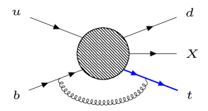
Figure 2: Loop contributions to single top production that need to be considered. We emphasise that there is no colour transfer from the light quark line to the heavy quark line, see text for details.

We write

$${\cal A}_{\rm virt}=g_{s}^{2}C_{F}\delta_{ij}{\cal M}_{\rm virt},$$ (32)

where $i,j$ are the colour indices of the top quark and the bottom quark. We note that the one-loop corrections to the “heavy” line can be written as the sum of four contributions (see Fig. 2)

$${\cal M}_{\rm virt}=\sum\limits_{i\in\{a,b,c,d\}}{\cal M}^{(i)}_{\rm virt},$$ (33)

where

$$\begin{split}&{\cal M}_{\rm virt}^{(a)}=\int\frac{{\rm d}^{4}k}{(2\pi)^{4}}\frac{-i}{k^{2}-\lambda^{2}}\left[\bar{u}_{t}\gamma^{\alpha}\frac{({\not{p}}_{t}+{\not{k}}+m_{t})}{d_{t}}{\bf N}(p_{t}+k,p_{b}+k,..)\frac{({\not{p}}_{b}+{\not{k}})}{d_{b}}\gamma_{\alpha}u_{b}\right],\\ &{\cal M}_{\rm virt}^{(b)}=\int\frac{{\rm d}^{4}k}{(2\pi)^{4}}\frac{-i}{k^{2}-\lambda^{2}}\left[\bar{u}_{t}\gamma_{\alpha}\frac{({\not{p}}_{t}+{\not{k}}+m_{t})}{d_{t}}{\bf N}_{1g}^{\alpha}(p_{t}+k,p_{b},..,|-k)u_{b}\right],\\ &{\cal M}_{\rm virt}^{(c)}=\int\frac{{\rm d}^{4}k}{(2\pi)^{4}}\frac{-i}{k^{2}-\lambda^{2}}\left[\bar{u}_{t}{\bf N}^{\alpha}_{1g}(p_{t},p_{b}+k,..,|k)\frac{({\not{p}}_{b}+{\not{k}})}{d_{b}}\gamma_{\alpha}u_{b}\right],\\ &{\cal M}_{\rm virt}^{(d)}=\int\frac{{\rm d}^{4}k}{(2\pi)^{4}}\frac{-ig_{\alpha\beta}}{k^{2}-\lambda^{2}}\left[\bar{u}_{t}{\bf N}_{2g}^{\alpha\beta}(p_{t},p_{b},..|k,-k)u_{b}\right].\end{split}$$ (34)

By a slight abuse of notation, we use $d_{b}=(p_{b}+k)^{2}$ in this section, and we continue to denote the external spinors as $\bar{u}_{t}=\bar{u}_{t}(p_{t})$ and $u_{b}=u_{b}(p_{b})$. The quantities ${\bf N}(p_{t}+k,p_{b}+k,..)$, ${\bf N}_{1g}^{\alpha}(p_{t}+k,p_{b},..,|-k)$ and ${\bf N}_{2g}^{\alpha}(p_{t}+k,p_{b},..,|k,-k)$ are functions that contribute to processes where the corresponding number of gluons (from zero to two) are emitted. We note that these functions do not include contributions where gluons are emitted from the external ($t$ and $b$) legs; for this reason all of them have smooth $k\to 0$ limits. To compute the ${\cal O}(\lambda)$ contribution to the differential cross section only the $k\sim\lambda$ integration region is relevant; as a result, all these functions can be expanded in Taylor series at small $k$.

A simple power counting suggests that ${\cal M}_{\rm virt}^{(d)}$ cannot provide an ${\cal O}(\lambda)$ contribution and therefore can be neglected, the function ${\bf N}_{1g}$ is needed at $k=0$ and the function ${\bf N}$ is needed through linear terms in $k$. Hence, we can write

$${\bf N}(p_{t}+k,p_{b}+k,...)={\bf N}(p_{t},p_{b},...)+k_{\mu}D_{p}^{\mu}{\bf N}(p_{t},p_{b},...)+{\cal O}(k^{2}),$$ (35)

where

$$D_{p}^{\mu}=\frac{\partial}{\partial p_{t,\mu}}+\frac{\partial}{\partial p_{b,\mu}}.$$ (36)

The function ${\bf N}_{1g}$ needs to be known at $k=0$. Following the discussion of the real emission contribution (cf. eq. (8)), we find

$$\bar{u}_{t}{\bf N}_{1g}^{\alpha}(p_{t},p_{b},..|k=0)u_{b}=-\bar{u}_{t}D_{p}^{\alpha}{\bf N}u_{b}.$$ (37)

Eqs. (35, 37) are sufficient to write an approximate expression for the virtual corrections. The manipulations are nearly identical to what has been discussed in the context of the real emission contribution in the previous section. We obtain

$$\bar{u}_{t}\gamma^{\alpha}\frac{({\not{p}}_{t}+{\not{k}}+m_{t})}{d_{t}}=\bar{u}_{t}\left(J_{t}^{\alpha}+{\bf S}_{t}^{\alpha}\right),$$ (38)

and

$$\frac{({\not{p}}_{b}+{\not{k}})}{d_{b}}\gamma^{\alpha}u_{b}=\left(J_{b}^{\alpha}-{\bf S}_{b}^{\alpha}\right)u_{b},$$ (39)

where

$$J_{t}^{\alpha}=\frac{2p_{t}^{\alpha}+k^{\alpha}}{d_{t}},\;\;\;{\bf S}_{t}^{\alpha}=\frac{\sigma^{\alpha\beta}k_{\beta}}{d_{t}},$$ (40)

and

$$J_{b}^{\alpha}=\frac{2p_{b}^{\alpha}+k^{\alpha}}{d_{b}},\;\;\;{\bf S}_{b}^{\alpha}=\frac{\sigma^{\alpha\beta}k_{\beta}}{d_{b}}.$$ (41)

Using these expressions and keeping only those terms that can provide linear power corrections, we find

$$\begin{split}&{\cal M}_{\rm virt}=\int\frac{{\rm d}^{4}k}{(2\pi)^{4}}\frac{-i}{k^{2}-\lambda^{2}}\Bigg{[}J_{t}^{\alpha}J_{b,\alpha}\;\bar{u}_{t}\left({\bf N}(p_{t},p_{b},..)+k^{\mu}D_{p,\mu}{\bf N}(p_{t},p_{b},..)\right)u_{b}\\ &-J_{t}^{\alpha}\bar{u}_{t}{\bf N}(p_{t},p_{b},..){\bf S}_{b,\alpha}u_{b}+J_{b}^{\alpha}\bar{u}_{t}{\bf S}_{t,\alpha}{\bf N}(p_{t},p_{b},..)u_{b}-(J_{t}^{\alpha}+J_{b}^{\alpha})\bar{u}_{t}D_{p,\alpha}{\bf N}u_{b}\Bigg{]}.\end{split}$$ (42)

Similar to the case of the real emission corrections, the dependence on the loop momentum has been made explicit so that the integration over $k$ becomes possible. However, it is beneficial to compute the correction to the matrix element squared before integrating over $k$. We find

$$\begin{split}&\delta_{\rm virt}[{\cal M}{\cal M}^{+}]=\int\frac{{\rm d}^{4}k}{(2\pi)^{4}}\frac{-i}{k^{2}-\lambda^{2}}\Bigg{[}2J_{t}^{\alpha}J_{b,\alpha}F_{\rm LO}\\ &+J_{t}^{\alpha}J_{b,\alpha}k^{\mu}\;{\rm Tr}\left[({\not{p}}_{t}+m_{t})(D_{p,\mu}{\bf N}){\not{p}}_{b}\bar{{\bf N}}+({\not{p}}_{t}+m_{t}){\bf N}{\not{p}}_{b}(D_{p,\mu}){\bar{{\bf N}}}\right]\\ &-(J_{t}^{\alpha}+J_{b}^{\alpha}){\rm Tr}\left[({\not{p}}_{t}+m_{t})(D_{p,\alpha}{\bf N}){\not{p}}_{b}{\bar{{\bf N}}}+({\not{p}}_{t}+m_{t}){\bf N}{\not{p}}_{b}(D_{p,\alpha}{\bar{{\bf N}}})\right]\\ &+J_{b}^{\alpha}{\rm Tr}\left[[{\not{p}}_{t},{\bf S}_{t,\alpha}]{\bf N}{\not{p}}_{b}{\bar{{\bf N}}}\right]-J_{t}^{\alpha}{\rm Tr}\left[({\not{p}}_{t}+m_{t}){\bf N}[{\bf S}_{b,\alpha},{\not{p}}_{b}]{\bar{{\bf N}}}\right]\Bigg{]},\end{split}$$ (43)

where ${\cal M}={\cal M}_{0}+{\cal M}_{\rm virt}$. We can further simplify this expression following the steps already discussed in the context of the real emission contribution. Indeed, using

$$\begin{split}&[{\not{p}}_{t},{\bf S}_{t}^{\alpha}]=\left(J_{t}^{\alpha}k^{\nu}\frac{\partial}{\partial p_{t}^{\nu}}-\frac{\partial}{\partial p_{t,\alpha}}\right){\not{p}}_{t}=L_{t}^{\alpha}{\not{p}}_{t},\\ &[{\not{p}}_{b},{\bf S}_{b}^{\alpha}]=\left(J_{b}^{\alpha}k^{\nu}\frac{\partial}{\partial p_{b}^{\nu}}-\frac{\partial}{\partial p_{b,\alpha}}\right){\not{p}}_{b}=L_{b}^{\alpha}{\not{p}}_{b},\end{split}$$ (44)

we arrive at

$$\begin{split}&\delta[{\cal M}{\cal M}^{+}]_{\rm virt}=\int\frac{{\rm d}^{4}k}{(2\pi)^{4}}\frac{-i}{k^{2}-\lambda^{2}}\Bigg{[}2J_{t}^{\alpha}J_{b,\alpha}F_{\rm LO}\\ &+J_{t}^{\alpha}J_{b,\alpha}k^{\mu}\;{\rm Tr}\left[({\not{p}}_{t}+m_{t})(D_{p,\mu}{\bf N}){\not{p}}_{b}{\bar{{\bf N}}}+({\not{p}}_{t}+m_{t}){\bf N}{\not{p}}_{b}(D_{p,\mu}{{\bar{{\bf N}}}})\right]\\ &-(J_{t}^{\alpha}+J_{b}^{\alpha}){\rm Tr}\left[({\not{p}}_{t}+m_{t})(D_{p,\alpha}{\bf N}){\not{p}}_{b}{\bar{{\bf N}}}+({\not{p}}_{t}+m_{t}){\bf N}{\not{p}}_{b}(D_{p,\alpha}{\bar{{\bf N}}})\right]\\ &+J_{b}^{\alpha}{\rm Tr}\left[(L_{t,\alpha}{\not{p}}_{t}){\bf N}{\not{p}}_{b}{\bar{{\bf N}}}\right]+J_{t}^{\alpha}{\rm Tr}\left[({\not{p}}_{t}+m_{t}){\bf N}(L_{b,\alpha}{\not{p}}_{b}){\bar{{\bf N}}}\right]\Bigg{]}.\end{split}$$ (45)

To simplify this expression further, we take the terms $J_{(t,b)}^{\alpha}k^{\mu}\partial/\partial p_{t,b}^{\mu}$ from $L_{t,b}^{\alpha}$ and combine them with the similar terms in the second line of eq. (45). We finally obtain

$$\begin{split}&\delta[{\cal M}{\cal M}^{+}]_{\rm virt}=\int\frac{{\rm d}^{4}k}{(2\pi)^{4}}\frac{-i}{k^{2}-\lambda^{2}}\Bigg{[}2J_{t}^{\alpha}J_{b,\alpha}F_{\rm LO}\\ &+J_{t}^{\alpha}J_{b,\alpha}k^{\mu}\;D_{p,\mu}F_{\rm LO}-(J_{t}^{\alpha}+J_{b}^{\alpha})D_{p,\alpha}F_{\rm LO}\\ &+J_{t}^{\alpha}{\rm Tr}\left[(D_{p,\alpha}{\not{p}}_{t}){\bf N}{\not{p}}_{b}{\bar{{\bf N}}}\right]+J_{b}^{\alpha}{\rm Tr}\left[({\not{p}}_{t}+m_{t}){\bf N}(D_{p,\alpha}{\not{p}}_{b}){\bar{{\bf N}}}\right]\Bigg{]}.\end{split}$$ (46)

The loop momentum $k$ in the above expression is contained in the currents $J_{t,b}^{\mu}$ and also appears explicitly in a few terms. Hence, it becomes possible to integrate over $k$. The needed integrals are given in Appendix A. Finally, putting everything together, we obtain

$$\begin{split}{\cal T}_{\lambda}\left[\sigma_{V}\right]=&-\frac{\alpha_{s}C_{F}}{2\pi}\frac{\pi\lambda}{m_{t}}\int{\rm dLips}_{\rm LO}\Bigg{[}{\rm Tr}\left[{\not{p}}_{t}{\bf N}{\not{p}}_{b}{\bar{\bf N}}\right]\\ &+\left(\frac{2p_{t}p_{b}-m_{t}^{2}}{p_{t}p_{b}}-\frac{m_{t}^{2}}{p_{t}p_{b}}p_{b}^{\mu}D_{p,\mu}\right)F_{\rm LO}\Bigg{]},\end{split}$$ (47)

where we have introduced the notation ${\rm dLips}_{\rm LO}={\rm dLips}(p_{u},p_{b};p_{d},p_{t},p_{X})$.

4 Renormalisation contributions

The above result for the virtual corrections has to be supplemented with the renormalisation contributions. Two of them (the wave function renormalisation of the external top quark and the top quark mass counter-term in the pole-mass scheme) provide ${\cal O}(\lambda)$ corrections to the cross section.

The two renormalisation constants can be computed using standard methods and read

$$\begin{split}&Z_{m}=1+\frac{C_{F}g_{s}^{2}m_{t}^{-2\epsilon}\Gamma(1+\epsilon)}{(4\pi)^{d/2}}\left[-\frac{3}{\epsilon}-4+\frac{2\pi\lambda}{m_{t}}+{\cal O}\left(\frac{\lambda^{2}}{m_{t}^{2}}\right)\right],\\ &Z_{2}=1+\frac{C_{F}g_{s}^{2}m_{t}^{-2\epsilon}\Gamma(1+\epsilon)}{(4\pi)^{d/2}}\left[-\frac{1}{\epsilon}-4+4\ln\frac{m_{t}}{\lambda}+\frac{3\lambda\pi}{m_{t}}+{\cal O}\left(\frac{\lambda^{2}}{m_{t}^{2}}\right)\right].\end{split}$$ (48)

For the purpose of our discussion only the ${\cal O}(\lambda)$ contributions to $Z_{2}$ and $Z_{m}$ are relevant.

It is straightforward to add the wave function renormalisation contribution to the virtual corrections. The mass counter-term, on the other hand, is only relevant for the internal top quark lines. Since the relation between the bare mass $m_{0}$ and the pole mass $m_{t}$ is given by $m_{0}=Z_{m}m_{t}$, we find

$$\frac{1}{{\not{p}}_{t}-m_{0}}=\frac{1}{{\not{p}}_{t}-m_{t}-(Z_{m}-1)m_{t}}\approx\frac{1}{{\not{p}}_{t}-m_{t}}+(Z_{m}-1)m_{t}\frac{\partial}{\partial m_{t}}\frac{1}{{\not{p}}_{t}-m_{t}}$$ (49)

where

$${\cal T}_{\lambda}\left[(Z_{m}-1)\right]m_{t}=\frac{C_{F}\alpha_{s}}{2\pi}\pi\lambda.$$ (50)

Putting everything together, we find the following result for the renormalisation contributions to the cross section

$$\begin{split}{\cal T}_{\lambda}\left[\sigma_{\rm ren}\right]=\frac{\alpha_{s}C_{F}}{2\pi}\frac{\pi\lambda}{m_{t}}\int{\rm dLips}_{\rm LO}\Bigg{[}\frac{3}{2}F_{\rm LO}&+m_{t}{\rm Tr}\left[({\not{p}}_{t}+m_{t})\frac{\partial{\bf N}}{\partial m_{t}}{\not{p}}_{b}{\bar{{\bf N}}}\right]\\ &+m_{t}{\rm Tr}\left[({\not{p}}_{t}+m_{t}){\bf N}{\not{p}}_{b}\frac{\partial{\bar{{\bf N}}}}{\partial m_{t}}\right]\Bigg{]}.\end{split}$$ (51)

5 Redefining the mass

It is well known that the use of the pole quark mass in physical predictions is one of the sources of linear power corrections. Such corrections are artificial and can be removed by employing one of the many short-distance mass schemes tHooft:1973mfk ; Czarnecki:1997sz ; Beneke:1998rk ; Hoang:1999ye ; Hoang:2008yj instead; we will refer to masses in such schemes as $\tilde{m}_{t}$. Hence, we need to derive a formula that provides a change in the cross section due to the change of the top quark mass.

To do this, it is important to recognise that such a dependence arises for two distinct reasons: 1) the implicit dependence of the energies of the final state particles on $m_{t}$ and 2) the explicit dependence of the matrix element squared on this parameter.

The explicit dependence is computed by writing $m_{t}=\tilde{m}_{t}+\delta m_{t}$ in the function $F_{\rm LO}$. The corresponding change in the leading order cross section reads

$$\begin{split}\delta\sigma_{\rm mass}^{\rm expl}=&\delta m_{t}\int{\rm dLips}_{\rm LO}\frac{\partial F_{\rm LO}}{\partial m_{t}}\\ =&\delta m_{t}\int{\rm dLips}_{\rm LO}\;\left({\rm Tr}\left[{\bf 1}{\bf N}{\not{p}}_{b}{\bar{{\bf N}}}\right]+{\rm Tr}\left[({\not{p}}_{t}+m_{t})\left(\frac{\partial{\bf N}}{\partial m_{t}}{\not{p}}_{b}{\bar{{\bf N}}}+{\bf N}{\not{p}}_{b}\frac{\partial{\bar{{\bf N}}}}{\partial m_{t}}\right)\right]\right).\end{split}$$ (52)

To compute the change in the cross section caused by the implicit dependence of the energies of the final state particles on $m_{t}$, we redefine the momenta of the top quark and another final state particle that we take to be the outgoing down quark, and write

$$p_{d}=(1+\kappa){\tilde{p}}_{d},\;\;\;p_{t}={\tilde{p}}_{t}-\kappa{\tilde{p}}_{d}.$$ (53)

It follows that

$$p_{t}^{2}=m_{t}^{2}={\tilde{p}}_{t}^{2}-2\kappa{\tilde{p}}_{t}{\tilde{p}}_{d}.$$ (54)

Hence, if we choose

$$\kappa=-\frac{\delta m_{t}^{2}}{2\tilde{p}_{t}{\tilde{p}}_{d}},$$ (55)

the mass-shell condition for ${\tilde{p}}_{t}$ becomes

$${\tilde{p}}_{t}^{2}={\tilde{m}}_{t}^{2}=m_{t}^{2}-\delta m_{t}^{2}.$$ (56)

Following the discussion of the momenta mapping of the real emission contribution in Section 2 and adjusting it where necessary, we find

$${\rm dLips}\left(p_{u},p_{b},p_{d},p_{t},p_{X};m_{t}^{2}\right)={\rm dLips}\left(p_{u},p_{b},{\tilde{p}}_{d},{\tilde{p}}_{t},p_{X};{\tilde{m}}_{t}^{2}\right)\left(1+\kappa\right).$$ (57)

Finally, expanding the leading order amplitude squared we obtain the change of the cross section due to the implicit mass change

$$\begin{split}&\delta\sigma^{\rm impl}_{\rm mass}=\int{\rm dLips}\left(p_{u},p_{b},{\tilde{p}}_{d},{\tilde{p}}_{t},p_{X}\right)\left[\kappa+\kappa{\tilde{p}}_{d}^{\mu}\left(\frac{\partial}{\partial{\tilde{p}}_{d}^{\mu}}-\frac{\partial}{\partial{\tilde{p}}_{t}^{\mu}}\right)\right]F_{\rm LO}({\tilde{p}}_{t},{\tilde{p}}_{d},\ldots)\\ &=-\int{\rm dLips}\left(p_{u},p_{b},p_{d},p_{t},p_{X}\right)\frac{\delta m_{t}^{2}}{2p_{d}p_{t}}\left[1+p_{d}^{\mu}\left(\frac{\partial}{\partial p_{d}^{\mu}}-\frac{\partial}{\partial p_{t}^{\mu}}\right)\right]F_{\rm LO}(p_{t},p_{d},\ldots),\end{split}$$ (58)

where in the last step we have re-labelled the momenta ${\tilde{p}}_{t}\Rightarrow p_{t}$ and ${\tilde{p}}_{d}\Rightarrow p_{d}$. Although short-distance masses can be defined in many different ways tHooft:1973mfk ; Czarnecki:1997sz ; Beneke:1998rk ; Hoang:1999ye ; Hoang:2008yj , they should not contain a linear ${\cal O}(\lambda)$ term. Hence, for our purposes, it suffices to write

$$m_{t}={\tilde{m}}_{t}\left(1-\frac{C_{F}\alpha_{s}}{2\pi}\frac{\pi\lambda}{m_{t}}\right).$$ (59)

It follows that

$$\delta m_{t}=-m_{t}\;\frac{C_{F}\alpha_{s}}{2\pi}\frac{\pi\lambda}{m_{t}},\;\;\;\;\delta m_{t}^{2}=-2m_{t}^{2}\;\frac{C_{F}\alpha_{s}}{2\pi}\frac{\pi\lambda}{m_{t}}.$$ (60)

Putting everything together, we finally find the change of the cross section due to the mass shift

$$\begin{split}\sigma_{\rm LO}(m_{t})-\sigma_{\rm LO}({\tilde{m}}_{t})&=\delta\sigma^{\rm expl}_{\rm mass}+\delta\sigma^{\rm impl}_{\rm mass}=\frac{C_{F}\alpha_{s}}{2\pi}\frac{\pi\lambda}{m_{t}}\;\int{\rm dLips}_{\rm LO}\times\\ &\Bigg{[}\frac{m_{t}^{2}}{p_{d}p_{t}}\left[1+p_{d}^{\mu}\left(\frac{\partial}{\partial p_{d}^{\mu}}-\frac{\partial}{\partial p_{t}^{\mu}}\right)\right]F_{\rm LO}-m_{t}{\rm Tr}\left[{\bf 1}{\bf N}{\not{p}}_{b}{\bar{{\bf N}}}\right]\\ &-m_{t}{\rm Tr}\left[({\not{p}}_{t}+m_{t})\left(\frac{\partial{\bf N}}{\partial m_{t}}{\not{p}}_{b}{\bar{{\bf N}}}+{\bf N}{\not{p}}_{b}\frac{\partial{\bar{{\bf N}}}}{\partial m_{t}}\right)\right]\Bigg{]}.\end{split}$$ (61)

6 The final result for the cross section

We now collect all the relevant formulae. We begin with the NLO cross section expressed through the pole mass and write it in terms of the short-distance mass

$$\sigma=\sigma_{\rm LO}(m_{t})+\sigma_{R}+\sigma_{V}+\sigma_{\rm ren}=\sigma_{\rm LO}({\tilde{m}}_{t})+\delta\sigma_{\rm NLO},$$ (62)

where

$$\delta\sigma_{\rm NLO}=\sigma_{R}+\sigma_{V}+\sigma_{\rm ren}+\delta\sigma^{\rm expl}_{\rm mass}+\delta\sigma^{\rm impl}_{\rm mass}.$$ (63)

The individual contributions read

$$\begin{split}{\cal T}_{\lambda}\left[\delta\sigma^{\rm expl}_{\rm mass}+\delta\sigma^{\rm impl}_{\rm mass}\right]&=\frac{C_{F}\alpha_{s}}{2\pi}\frac{\pi\lambda}{m_{t}}\;\int{\rm dLips}_{\rm LO}\times\\ &\;\;\;\;\;\;\Bigg{[}\frac{m_{t}^{2}}{p_{d}p_{t}}\left[1+p_{d}^{\mu}\left(\frac{\partial}{\partial p_{d}^{\mu}}-\frac{\partial}{\partial p_{t}^{\mu}}\right)\right]F_{\rm LO}-m_{t}{\rm Tr}\left[{\bf 1}{\bf N}{\not{p}}_{b}{\bar{{\bf N}}}\right]\\ &\;\;\;\;\;-m_{t}{\rm Tr}\left[({\not{p}}_{t}+m_{t})\left(\frac{\partial{\bf N}}{\partial m_{t}}{\not{p}}_{b}{\bar{{\bf N}}}+{\bf N}{\not{p}}_{b}\frac{\partial{\bar{{\bf N}}}}{\partial m_{t}}\right)\right]\Bigg{]},\\ {\cal T}_{\lambda}\left[\sigma_{\rm R}\right]&=\frac{\alpha_{s}C_{F}}{2\pi}\frac{\pi\lambda}{m_{t}}\int{\rm dLips}_{\rm LO}\Bigg{[}\left(\frac{3}{2}-\frac{m_{t}^{2}}{p_{d}p_{t}}-\frac{m_{t}^{2}}{p_{t}p_{b}}\right)\\ &\;\;\;\;-\frac{m_{t}^{2}}{p_{d}p_{t}}{p}_{d}^{\mu}\left(\frac{\partial}{\partial{p}_{d}^{\mu}}-\frac{\partial}{\partial{p}_{t}^{\mu}}\right)-\frac{m_{t}^{2}}{{p}_{t}{p}_{b}}p_{b}^{\mu}D_{p,\mu}\Bigg{]}F_{\rm LO},\\ {\cal T}_{\lambda}\left[\sigma_{V}\right]&=-\frac{\alpha_{s}C_{F}}{2\pi}\frac{\pi\lambda}{m_{t}}\int{\rm dLips}_{\rm LO}\Bigg{[}{\rm Tr}\left[{\not{p}}_{t}{\bf N}{\not{p}}_{b}{\bar{{\bf N}}}\right]\\ &\;\;\;\;\;+\left(\frac{(2p_{t}p_{b}-m_{t}^{2})}{p_{t}p_{b}}-\frac{m_{t}^{2}}{p_{t}p_{b}}\;p_{b}^{\mu}D_{p,\mu}\right)F_{\rm LO}\Bigg{]},\\ {\cal T}_{\lambda}\left[\sigma_{\rm ren}\right]&=\frac{\alpha_{s}C_{F}}{2\pi}\frac{\pi\lambda}{m_{t}}\int{\rm dLips}_{\rm LO}\Bigg{[}\frac{3}{2}F_{\rm LO}\\ &\;\;\;\;+m_{t}{\rm Tr}\left[({\not{p}}_{t}+m_{t})\frac{\partial{\bf N}}{\partial m_{t}}{\not{p}}_{b}{\bar{{\bf N}}}\right]+m_{t}{\rm Tr}\left[({\not{p}}_{t}+m_{t}){\bf N}{\not{p}}_{b}\frac{\partial{\bar{{\bf N}}}}{\partial m_{t}}\right]\Bigg{]}.\end{split}$$ (64)

Using the above results for the individual contributions, we obtain

$$\begin{split}{\cal T}_{\lambda}\left[\delta\sigma_{\rm NLO}\right]&=\frac{\alpha_{s}C_{F}}{2\pi}\frac{\pi\lambda}{m_{t}}\int{\rm dLips}_{\rm LO}\;\left(F_{\rm LO}-{\rm Tr}\left[{\not{p}}_{t}{\bf N}{\not{p}}_{b}{\bar{{\bf N}}}\right]-m_{t}{\rm Tr}\left[{\bf 1}{\bf N}{\not{p}}_{b}{\bar{{\bf N}}}\right]\right)=0.\end{split}$$ (65)

This result implies that ${\cal O}(\Lambda_{\rm QCD})$ corrections to processes where single top quarks are produced by virtue of weak flavor-changing interactions vanish provided that the cross section is expressed in terms of the short-distance top quark mass. In Appendix B we explain how our method can be used to re-derive the known result that there are no ${\cal O}(\Lambda_{\rm QCD})$ corrections to semileptonic decays of a heavy quark Bigi:1994em ; Beneke:1994bc .

7 Alternative treatment of the self-energy corrections

The previous computation was first carried out in the pole-mass scheme, and then a scheme change was performed to get the result in an arbitrary short distance scheme. Alternatively, it is possible to perform the calculation directly in a short distance scheme. In order to do that, we consider the squared amplitude directly and recall that the external top quark line is represented by

$$2\pi({\not{p}}_{t}+m_{t})\delta(p_{t}^{2}-m_{t}^{2})={\rm Disc}\left[\frac{1}{{\not{p}}_{t}-m_{t}}\right]\equiv\left[\frac{i}{{\not{p}}_{t}-m_{t}+i\epsilon}-\frac{i}{{\not{p}}_{t}-m_{t}-i\epsilon}\right]\,,$$ (66)

One then deals with this external line in the same way as one deals with internal lines in Feynman diagrams, namely one inserts the self-energy correction and the mass counter-term into the argument of the ${\rm Disc}$ function, but the wave function renormalisation does not need to be included. If the mass is renormalised in any short-distance scheme, we do not need to include the mass counter-term either, since it does not contain terms linear in $\lambda$. For the same reason, mass counter-terms in the internal top quark lines are not needed. Thus, we can simply compute the self-energy insertion without including any counter-term. The self-energy correction is given by

$$\frac{i}{{\not{p}}_{t}-m_{t}}i\Sigma\frac{i}{{\not{p}}_{t}-m_{t}},$$ (67)

where

$$i\Sigma=C_{F}g_{s}^{2}\int\frac{\mathrm{d}^{4}k}{(2\pi)^{4}}\frac{-i}{k^{2}-\lambda^{2}+i\epsilon}(-i\gamma_{\mu})\frac{i}{{\not{p}}_{t}-{\not{k}}-m_{t}+i\epsilon}(-i\gamma^{\mu}).$$ (68)

We need to evaluate $\Sigma$ up to terms that are suppressed by more than one power of ${\not{p}}_{t}-m_{t}$, since higher powers do not contribute to the discontinuity. Making use of the virtual integrals given in Appendix A, a straightforward calculation yields

$$\begin{split}{\cal T}_{\lambda}\left[\Sigma\right]&=C_{F}g_{s}^{2}\left[\frac{1}{8m_{t}}(p_{t}^{2}-m_{t}^{2})+\frac{2m_{t}-{\not{p}}_{t}}{2}\right]\frac{1}{(2\pi)^{2}}\frac{\lambda\pi}{\sqrt{p_{t}^{2}}}\\ &=\frac{\alpha_{s}C_{F}}{2\pi}\frac{\lambda\pi}{m_{t}}\left[-\frac{1}{4m_{t}}(p_{t}^{2}-m_{t}^{2})+2m_{t}-{\not{p}}_{t}\right]\,.\end{split}$$ (69)

The full correction can be written as

$$\begin{split}{\cal T}_{\lambda}\left[{\rm Disc}\left[\left(\frac{i}{{\not{p}}_{t}-m_{t}}\right)^{2}\Sigma\right]\right]&=\frac{\alpha_{s}C_{F}}{2\pi}\frac{\lambda\pi}{m_{t}}\,\Bigg{[}\frac{3}{2}({\not{p}}_{t}+m_{t})\,2\pi\,\delta(p_{t}^{2}-m_{t}^{2})\\ &-m_{t}2\pi\,\delta(p_{t}^{2}-m_{t}^{2})+2m_{t}^{2}(m_{t}+{\not{p}}_{t})\delta^{\prime}(p_{t}^{2}-m_{t}^{2})\Bigg{]},\end{split}$$ (70)

where $\delta^{\prime}(p_{t}^{2}-m_{t}^{2})$ is the derivative of the $\delta$-function with respect to $p_{t}^{2}$. In order to handle this derivative, we rewrite it as

$$\begin{split}\delta^{\prime}(p_{t}^{2}-m_{t}^{2})&=\frac{p_{d}^{\mu}}{2p_{d}p_{t}}\,\frac{\partial}{\partial p_{t}^{\mu}}\delta(p_{t}^{2}-m_{t}^{2})=-\delta(p_{t}^{2}-m_{t}^{2})\frac{\partial}{\partial p_{t}^{\mu}}\frac{p_{d}^{\mu}}{2p_{d}p_{t}}\\ &=\delta(p_{t}^{2}-m_{t}^{2})\left[\frac{4}{2p_{d}p_{t}}+\frac{p_{d}^{\mu}}{2(p_{d}p_{t})^{2}}[-{p}_{t,\mu}+{p}_{b,\mu}]-\frac{p_{d}^{\mu}}{2p_{d}p_{t}}\frac{\partial}{\partial p_{t}^{\mu}}\right]\\ &=\delta(p_{t}^{2}-m_{t}^{2})\left[\frac{3}{2p_{d}p_{t}}-\frac{p_{d}^{\mu}}{2p_{d}p_{t}}\frac{\partial}{\partial p_{t}^{\mu}}\right]\,,\end{split}$$ (71)

where we have integrated by parts, and we have assumed that in the phase space $p_{d}$ is taken as the dependent momentum, i.e. $p_{d}=p_{u}+p_{b}-p_{X}-p_{t}$. The remaining derivative with respect to $p_{t}$ can be applied to the amplitude or to the delta-function $\delta(p_{d}^{2})$ in the phase space. In the second case we get

$$-\frac{p_{d}^{\mu}}{2p_{d}p_{t}}\frac{\partial}{\partial p_{t}^{\mu}}\;\delta(p_{d}^{2})=\frac{1}{p_{d}p_{t}}\,p_{d}^{2}\delta^{\prime}(p_{d}^{2})=-\frac{1}{2p_{d}p_{t}}\delta(p_{d}^{2}).$$ (72)

Thus, in eq. (70) we can replace

$$\delta^{\prime}(p_{t}^{2}-m_{t}^{2})\Rightarrow\delta(p_{t}^{2}-m_{t}^{2})\left[\frac{1}{2p_{d}p_{t}}-\frac{p_{d}^{\mu}}{2p_{d}p_{t}}\frac{\partial}{\partial p_{t}^{\mu}}\right]\,,$$ (73)

with an understanding that the derivative acts only on the amplitude squared. Inserting eq. (70) in the spinor trace, and including the phase space we get

$$\delta\sigma_{\rm self}=\frac{\alpha_{s}C_{F}}{2\pi}\frac{\lambda\pi}{m_{t}}\int\mathrm{d}{\rm Lips}_{\rm LO}\left[\frac{3}{2}F_{\rm LO}-m_{t}{\rm Tr}[{\bf 1}{\bf N}{\not{p}}_{b}{\bar{{\bf N}}}]-\frac{m_{t}^{2}}{p_{d}{p}_{t}}\left(p_{d}^{\mu}\frac{\partial F_{\rm LO}}{\partial p_{t}^{\mu}}-F_{\rm LO}\right)\right].$$ (74)

In case $p_{d}$ is treated as an independent variable we must replace

$$\frac{\partial}{\partial p_{t}^{\mu}}\to\frac{\partial}{\partial p_{t}^{\mu}}-\frac{\partial}{\partial p_{d}^{\mu}}\,,$$ (75)

and eq. (74) becomes equivalent to the sum of the renormalisation contributions of eq. (51) and the mass shift of eq. (61).

8 Kinematic distributions

We will now study kinematic distributions in the single top production processes. We consider an observable $X$ that depends on the momentum of the top quark

$$O_{X}=\int{\rm d}\sigma\;X(q_{t}).$$ (76)

To compute the ${\cal O}(\lambda)$ contribution to $O_{X}$, we follow the same route that was discussed in the previous sections. The difference with respect to the case of the inclusive cross section is the appearance of the observable $X$ in the integrand in eq. (76). Remapping the momenta, and expanding $X$ in the gluon momentum $k$, which appears in the argument of $X$ as the result of such remapping, we obtain

$$X(q_{t})=X(p_{t})+\frac{\partial X(p_{t})}{\partial p_{t}^{\mu}}\left(\frac{p_{t}k}{p_{t}p_{d}}p_{d}^{\mu}-k^{\mu}\right).$$ (77)

To compute the ${\cal O}(\lambda)$ contributions to $O_{X}$ it is convenient to combine the three terms in eq. (77) as follows

$${\cal T}_{\lambda}[O_{X}]={\cal T}_{\lambda}[O^{(1)}_{X}]+{\cal T}_{\lambda}[O^{(2)}_{X}],$$ (78)

where

$$\begin{split}&{\cal T}_{\lambda}[O^{(1)}_{X}]={\cal T}_{\lambda}\left[\int{\rm d}\sigma\;\left(X(p_{t})+\frac{\partial X(p_{t})}{\partial p_{t}^{\mu}}\;\frac{p_{t}k}{p_{t}p_{d}}p_{d}^{\mu}\right)\right],\\ &{\cal T}_{\lambda}[O^{(2)}_{X}]=-{\cal T}_{\lambda}\left[\int{\rm d}\sigma\;\frac{\partial X(p_{t})}{\partial p_{t}^{\mu}}\;k^{\mu}\right].\end{split}$$ (79)

To compute ${\cal T}_{\lambda}[O^{(1)}_{X}]$, we note that the observable $X(p_{t})$ that appears there already depends on the re-mapped momentum $p_{t}$ and, for this reason, it does not affect the calculations reported in the previous sections and the cancellation of ${\cal O}(\lambda)$ terms. The only subtlety is that the mass redefinition in eq. (58) produces an additional term because in the current case the derivative there must also act on $X$. However, it is easy to see that this new term is exactly compensated by the integral of the $k$-dependent term in the integrand of ${\cal T}_{\lambda}[O^{(1)}_{X}]$. We conclude that

$${\cal T}_{\lambda}[O_{X}^{(1)}]=0.$$ (80)

It remains to compute ${\cal T}_{\lambda}[O_{X}^{(2)}]$. Since the integrand is already proportional to $k$, we need the matrix element squared and the phase space in the leading soft approximation. We therefore find

$${\cal T}_{\lambda}[O_{X}^{(2)}]={\cal T}_{\lambda}\left[C_{F}g_{s}^{2}\int{\rm d}\sigma_{\rm LO}\frac{\partial X(p_{t})}{\partial p_{t}^{\mu}}\int\frac{{\rm d}^{4}k}{(2\pi)^{3}}\,\delta_{+}(k^{2}-\lambda^{2})\;J^{\nu}J_{\nu}\;k^{\mu}\right],$$ (81)

where the eikonal current $J^{\nu}$ reads

$$J^{\nu}\approx\frac{p_{t}^{\nu}}{p_{t}k}-\frac{p_{b}^{\nu}}{p_{b}k}.$$ (82)

Using earlier discussions and the integrals presented in Appendix A, it is straightforward to integrate this expression over $k$. We obtain

$${\cal T}_{\lambda}\left[O_{X}\right]={\cal T}_{\lambda}\left[O_{X}^{(2)}\right]=\frac{\alpha_{s}C_{F}}{2\pi}\frac{\pi\lambda}{m_{t}}\;\int{\rm d}\sigma_{\rm LO}\;l^{\mu}\frac{\partial X(p_{t})}{\partial p_{t}^{\mu}},$$ (83)

where

$$l^{\mu}=p_{t}^{\mu}-\frac{2m_{t}^{2}}{p_{b}p_{t}}p_{b}^{\mu}.$$ (84)

Using the alternative procedure for the inclusion of the self-energy corrections in Section 7 we immediately reach the same conclusion, except that the cancellation of the second term of eq. (77) arises from the derivative term in eq. (74) by replacing $F_{\rm LO}$ with $X\,F_{\rm LO}$, so that the derivative that hits $F_{\rm LO}$ there can now also act on $X(p_{t})$.

The result of eq. (83) can be interpreted as a non-perturbative shift in the argument of the observable $X(p_{t})$. Indeed, we can write

$$\begin{split}O_{X}&=\int{\rm d}\sigma_{\rm LO}\left[X(p_{t})+\frac{\alpha_{s}C_{F}}{2\pi}\frac{\pi\lambda}{m_{t}}\;l^{\mu}\frac{\partial X(p_{t})}{\partial p_{t}^{\mu}}\right]\\ &=\int{\rm d}\sigma_{\rm LO}\;X\left(p_{t}+\frac{\alpha_{s}C_{F}}{2\pi}\delta p_{t}\right),\end{split}$$ (85)

where

$$\delta p_{t}=\frac{\pi\lambda}{m_{t}}\;l.$$ (86)

As an example, suppose that $X$ is a function of the transverse momentum distribution of the top quark, such as, for example, a cut on the transverse momentum, or a product of theta functions singling out a particular histogram bin. In this case

$${p_{t}}_{\perp}=\sqrt{|p_{t}^{\mu}g_{\perp,\mu\nu}p_{t}^{\nu}|},$$ (87)

where

$$g_{\perp}^{\mu\nu}=g^{\mu\nu}-\frac{p_{b}^{\mu}p_{u}^{\nu}+p_{u}^{\mu}p_{b}^{\nu}}{p_{u}p_{b}}.$$ (88)

Since $p_{b}^{\mu}g_{\perp,\mu\nu}=0$, we find

$$\frac{\delta_{\rm NP}\left[\;{p_{t}}_{\perp}\right]}{{p_{t}}_{\perp}}=\frac{\alpha_{s}C_{F}}{2\pi}\frac{\pi\lambda}{m_{t}}.$$ (89)

It is interesting to point out that the relative non-perturbative shift in ${p_{t}}_{\perp}$ and the relative non-perturbative shift in the top quark mass coincide

$$\frac{\delta_{\rm NP}\left[\;{p_{t}}_{\perp}\right]}{{p_{t}}_{\perp}}=\frac{\delta_{\rm NP}[m_{t}]}{m_{t}}.$$ (90)

Since the non-perturbative uncertainty in the top quark mass is estimated as $100-200~{}{\rm MeV}$ Beneke:2016cbu ; Schwienhorst:2022yqu ; Hoang:2017btd , we conclude that the non-perturbative shift in the top quark transverse momentum reads

$$\delta_{\rm NP}\left[\;{p_{t}}_{\perp}\right]\approx(0.1-0.2)~{}\frac{{p_{t}}_{\perp}}{m_{t}}~{}{\rm GeV}.$$ (91)

The transverse momentum distribution of the $t$-channel single top production is peaked around $50~{}{\rm GeV}$; for such momenta, the non-perturbative shift is very small, ${\cal O}(30-60)$ MeV.

Another observable to consider is the top quark rapidity distribution. In the partonic center of mass frame, it reads

$$y_{t}=\frac{1}{2}\ln\frac{p_{b}p_{t}}{p_{u}p_{t}}.$$ (92)

An easy computation gives

$$\begin{split}&\delta_{\rm NP}\left[y_{t}\right]=\frac{\alpha_{s}C_{F}}{2\pi}\frac{\pi\lambda}{m_{t}}\;l^{\mu}\;\frac{1}{2}\left(\frac{p_{b}^{\mu}}{p_{b}p_{t}}-\frac{p_{u}^{\mu}}{p_{u}p_{t}}\right)\\ &=\frac{\alpha_{s}C_{F}}{2\pi}\frac{\pi\lambda}{m_{t}}\frac{(p_{u}p_{b})m_{t}^{2}}{(p_{u}p_{t})(p_{b}p_{t})}=\frac{\alpha_{s}C_{F}}{2\pi}\frac{\pi\lambda}{m_{t}}\frac{8m_{t}^{2}s\,{\rm ch}^{2}(y_{t})}{(s+m_{t}^{2})^{2}}.\end{split}$$ (93)

9 Conclusions

In this paper we discussed the non-perturbative ${\cal O}(\Lambda_{\rm QCD})$ corrections to electroweak production of a single top quark in hadronic collisions in the context of renormalon calculus. Processes of the type $pp\to q+t+X$, where $X$ is an arbitrary collection of colour-neutral particles, can be studied in the framework of renormalon calculus because such processes do not contain gluons in leading order diagrams.

We have shown how to use Low-Burnett-Kroll theorem, which allows one to express sub-leading contributions in the soft expansion in a process-independent way, to analyse ${\cal O}(\Lambda_{\rm QCD})$ corrections to arbitrary processes of a single top production type. Our findings are remarkably simple. Indeed, we observe that total cross sections for such processes have no linear power corrections provided that a short-distance mass scheme is used to compute them. Therefore, if a total cross section is employed to determine the top quark mass, it is more natural to use a short-distance mass scheme since, by doing so, we avoid the presence of linear renormalons. Since renormalons are associated with the factorial growth of the coefficients in perturbative series, the absence of linear renormalons should lead to a better convergence of the perturbative expansion in a short-distance mass scheme. Although these conclusions appear to be quite natural given what is known about semileptonic decays of heavy quarks, our calculation provides a strong indication of the absence of ${\cal O}(\Lambda_{\rm QCD})$ corrections to one of the main top quark production processes at a hadron collider. Although these results are obtained in the context of the renormalon calculus, we hope that they remain valid also in full QCD.

We have also discussed how to generalise these results to compute linear power corrections to kinematic distributions that involve the top quark momentum. In this case, using a short-distance mass scheme and making use of the pattern of cancellations of various ${\cal O}(\lambda)$ contributions which becomes apparent from the discussion of the total cross section, very simple formulae for ${\cal O}(\Lambda_{\rm QCD})$ non-perturbative shifts in the transverse momentum and rapidity distributions of the top quark can be derived.

An important shortcoming of the approach to non-perturbative effects in single top production developed in this paper is that it applies to stable top quarks. Since all ${\cal O}(\Lambda_{\rm QCD})$ corrections computed in this paper come from kinematic regions where top quarks are nearly on shell, the instability of the top quark should have a major effect on these results, suppressing linear power corrections in realistic kinematic distributions. In a related context, an interplay between the instability of the top quark and ${\cal O}(\Lambda_{\rm QCD})$ corrections were studied numerically in ref. FerrarioRavasio:2018ubr . In the future, it would be interesting to investigate this interplay in more detail and establish the degree of suppression of linear power corrections that otherwise appear in various kinematic distributions.

Appendix A Loop and real-emission integrals required for computing linear power corrections

In this appendix we present the results for the various integrals that arise in the course of the calculations reported in this paper. To write the results for these integrals in a compact way, we introduce a variable

$$\delta=\frac{1}{(2\pi)^{2}}\frac{\lambda\pi}{m_{t}}.$$ (94)

A.1 Real emission integrals

The computation of the real emission integrals can be performed in the top quark rest frame, with an arbitrary upper cutoff on the energy of the emitted gluon. The result does not depend upon the chosen frame, since the only frame dependence can arise from the upper cutoff, and the soft region is not affected by it. Thus one replaces

$$\int\frac{{\rm d}^{4}k}{(2\pi)^{3}}\delta_{+}(k^{2}-\lambda^{2})\Rightarrow\int_{\lambda}^{w_{\rm max}}\frac{\beta\omega\mathrm{d}\omega}{2(2\pi)^{4}}\int\mathrm{d}\varphi\,\int\mathrm{d}\cos\theta,$$ (95)

where $\omega$ is the top quark energy, the polar axis is chosen along the direction of a $b$ quark and $\beta=\sqrt{1-{\lambda^{2}}/{\omega^{2}}}$, all in the top quark rest frame. All integrals are elementary; in the worst case one encounters integrals of the form

$$\int_{\lambda}^{w_{\rm max}}\frac{\mathrm{d}\omega}{\omega^{k}}\,\log\frac{1+\beta}{1-\beta}$$ (96)

that are easily done by parts, since

$$\frac{\mathrm{d}}{\mathrm{d}\omega}\log\frac{1+\beta}{1-\beta}=\frac{2}{\sqrt{\omega^{2}-\lambda^{2}}}.$$ (97)

The integrals required for computing the real emission contribution to single top production read

$$I_{1}={\cal T}_{\lambda}\left[\int\frac{{\rm d}^{4}k}{(2\pi)^{3}}\delta_{+}(k^{2}-\lambda^{2})\;\frac{\lambda^{2}}{(2p_{t}k)^{3}}\right]=\frac{1}{32m_{t}^{2}}\;\delta,$$ (98)

$$I_{2}={\cal T}_{\lambda}\left[\int\frac{{\rm d}^{4}k}{(2\pi)^{3}}\delta_{+}(k^{2}-\lambda^{2})\;\frac{k^{\mu}}{(2p_{t}k)^{2}}\right]=-\frac{p^{\mu}_{t}}{8m_{t}^{2}}\delta,$$ (99)

$$I_{3}={\cal T}_{\lambda}\left[\int\frac{{\rm d}^{4}k}{(2\pi)^{3}}\delta_{+}(k^{2}-\lambda^{2})\;\frac{1}{(2p_{t}k)^{2}}\right]=0,$$ (100)

$$I_{4}={\cal T}_{\lambda}\left[\int\frac{{\rm d}^{4}k}{(2\pi)^{3}}\delta_{+}(k^{2}-\lambda^{2})\;\frac{\lambda^{2}}{(2p_{t}k)^{2}(-2p_{b}k)}\right]=-\frac{1}{16(p_{t}p_{b})}\delta,$$ (101)

$$I_{5}={\cal T}_{\lambda}\left[\int\frac{{\rm d}^{4}k}{(2\pi)^{3}}\delta_{+}(k^{2}-\lambda^{2})\;\frac{\lambda^{2}}{(2p_{t}k)(-2p_{b}k)^{2}}\right]=-\frac{m_{t}^{2}}{16(p_{t}p_{b})^{2}}\delta,$$ (102)

$$I_{6}={\cal T}_{\lambda}\left[\int\frac{{\rm d}^{4}k}{(2\pi)^{3}}\delta_{+}(k^{2}-\lambda^{2})\;\frac{k^{\mu}}{(2p_{t}k)(-2p_{b}k)}\right]=\frac{1}{8(p_{t}p_{b})}\left(p_{t}^{\mu}-\frac{m_{t}^{2}}{p_{t}p_{b}}\;p_{b}^{\mu}\right)\delta.$$ (103)

A.2 Loop integrals

The required loop integrals read

$${\cal T}_{\lambda}\left[-i\int\frac{{\rm d}^{4}k}{(2\pi)^{4}(k^{2}-\lambda^{2})}J_{t}^{\mu}J_{b,\mu}\right]=\frac{1}{(4\pi)^{2}}\frac{m_{t}^{2}-2p_{t}p_{b}}{p_{t}p_{b}}\frac{\pi\lambda}{m_{t}},$$ (104)

$${\cal T}_{\lambda}\left[-i\int\frac{{\rm d}^{4}k}{(2\pi)^{4}(k^{2}-\lambda^{2})}J_{t}^{\alpha}J_{b,\alpha}k^{\mu}\right]=-\frac{2}{(4\pi)^{2}}\frac{\pi\lambda}{m_{t}}\left(p_{t}^{\mu}-\frac{m_{t}^{2}}{p_{t}p_{b}}p_{b}^{\mu}\right),$$ (105)

$${\cal T}_{\lambda}\left[-i\int\frac{{\rm d}^{4}k}{(2\pi)^{4}(k^{2}-\lambda^{2})}J_{t}^{\mu}\right]=-\frac{2}{(4\pi)^{2}}\frac{\pi\lambda}{m_{t}}\;p_{t}^{\mu},$$ (106)

$${\cal T}_{\lambda}\left[-i\int\frac{{\rm d}^{4}k}{(2\pi)^{4}(k^{2}-\lambda^{2})}J_{b}^{\mu}\right]=0.$$ (107)

To compute them, we integrate over $k_{0}$ and map them onto real emission integrals. More precisely, we first perform the replacement $k\rightarrow-k$ and then perform the $k^{0}$ integration in the $p_{t}$ rest frame. The poles of the $k^{2}-\lambda^{2}$, $d_{b}$ and $d_{t}$ denominators are given by

$$\omega =\pm\sqrt{\vec{k}^{2}+\lambda^{2}}\mp i\epsilon,$$ (108)

$$\omega =p_{b}^{0}\pm\sqrt{(p_{b}^{0})^{2}+(2\vec{k}\vec{p}_{b}+\vec{k}^{2})}\mp i\epsilon,$$ (109)

$$\omega =m\pm\sqrt{m^{2}+\vec{k}^{2}}\mp i\epsilon,$$ (110)

where $\omega=k^{0}$. We see that if we close the contour in the lower complex plane we pick the residues of the poles with the upper signs in eqs. (108-110), i.e. the poles with negative imaginary part, but only the pole in eq. (108) leads to a small value of $\omega$, and thus leads to a term sensitive to $\lambda$. Thus we can replace

$$i\int\frac{{\rm d}^{4}k}{(2\pi)^{4}(k^{2}-\lambda^{2})}\Rightarrow\int\frac{{\rm d}^{4}k}{(2\pi)^{3}}\theta(k^{0})\delta(k^{2}-\lambda^{2})\,,$$ (111)

and then use the already known results for the real emission integrals.

Appendix B Semileptonic decays of a heavy quark

In this section we consider the semileptonic decay of a top quark into a massless bottom quark and an arbitrary collection of colour-neutral particles, $t\to b+X$. We will re-derive a well-known result Bigi:1994em ; Beneke:1994bc that there are no ${\cal O}(\lambda)$ contributions to the total decay width $\Gamma(t\to b+X)$ provided that the width is expressed in terms of a short-distance mass of the top quark.

We note that all major steps of the calculation that we discussed in the context of the single top production remain valid also for the semileptonic decay. In particular, the calculation of the contribution of the virtual corrections is identical. The renormalisation procedure also remains the same. As a result, we find

$$\begin{split}&{\cal T}_{\lambda}\left[m_{t}\;\Gamma_{V+\rm ren}\right]=-\frac{\alpha_{s}C_{F}}{2\pi}\frac{\pi\lambda}{m_{t}}\int{\rm dLips}(p_{t}|p_{b},...)\Bigg{[}{\rm Tr}\left[{\not{p}}_{b}{\bf N}{\not{p}}_{t}{\bar{{\bf N}}}\right]\\ &-m_{t}{\rm Tr}\left[{\not{p}}_{b}\frac{\partial{\bf N}}{\partial m_{t}}({\not{p}}_{t}+m_{t}){\bar{{\bf N}}}\right]-m_{t}{\rm Tr}\left[{\not{p}}_{b}{\bf N}({\not{p}}_{t}+m_{t})\frac{\partial{\bar{{\bf N}}}}{\partial m_{t}}\right]\\ &+\left(-\frac{3}{2}+\frac{(2p_{t}p_{b}-m_{t}^{2})}{p_{t}p_{b}}-\frac{m_{t}^{2}}{p_{t}p_{b}}\;p_{b}^{\mu}D_{p,\mu}\right)F^{(d)}_{\rm LO}\Bigg{]},\end{split}$$ (112)

where $F^{(d)}_{\rm LO}={\rm Tr}\left[{\not{p}}_{b}{\bf N}({\not{p}}_{t}+m_{t}){\bar{{\bf N}}}\right]$ is the leading order invariant amplitude squared. We also note that the above result is written for the product of the top quark mass $m_{t}$ and the decay width, that is proportional to the squared amplitude up to a numeric factor that is irrelevant for the present purposes. We will see that it is $\Gamma$, rather than the invariant amplitude, that is free of linear renormalons if expressed in terms of a short-distance mass.

The calculation of the real-emission contributions proceeds similarly to the case of the single top production. In particular, an application of Low-Burnett-Kroll theorem leads again to eq. (23) where for the decay

$$\begin{split}&J^{\mu}=J_{t}^{\mu}+J_{b}^{\mu},\\ &J_{t}^{\mu}=\frac{2p_{t}^{\mu}-k^{\mu}}{d_{t}},\;\;\;\;J_{b}^{\mu}=\frac{2p_{b}^{\mu}+k^{\mu}}{d_{b}},\end{split}$$ (113)

with $d_{t}=(p_{t}-k)^{2}-m_{t}^{2}$ and $d_{b}=(p_{2}+k)^{2}$.

In order to factorise the integration over the gluon momentum from the rest of the phase space, a momentum mapping is needed. This mapping differs from the one employed in the discussion of the single top production. We map the momentum of one of the colour-neutral, massless final-state particles (with momentum $p_{3}$) and the $b$-quark as follows

$$\begin{split}&p_{b}=\tilde{p}_{b}-k+\frac{\tilde{p}_{b}k}{\tilde{p}_{3}\tilde{p}_{b}}\tilde{p}_{3},\;\;\;\;p_{3}=\left(1-\frac{\tilde{p}_{b}k}{\tilde{p}_{3}\tilde{p}_{b}}\right)\tilde{p}_{3}.\end{split}$$ (114)

Upon this transformation, the phase space changes as follows

$${\rm dLips}(p_{t}|p_{b},p_{3},k,...)={\rm dLips}(p_{t}|\tilde{p}_{b},\tilde{p}_{3},..)\frac{{\rm d}^{4}k}{(2\pi)^{4}}\delta(k^{2}-\lambda^{2})\left(1+\frac{k\tilde{p}_{3}}{\tilde{p}_{b}\tilde{p}_{3}}-\frac{k\tilde{p}_{b}}{\tilde{p}_{b}\tilde{p}_{3}}\right).$$ (115)

Integrating over the gluon momentum $k$ using the integrals in Appendix A, we obtain the real emission contribution

$$\begin{split}&{\cal T}_{\lambda}\left[m_{t}\;\Gamma_{\rm R}\right]=\frac{\alpha_{s}C_{F}}{2\pi}\frac{\pi\lambda}{m_{t}}\int{\rm dLips}(p_{t},\tilde{p}_{b},\tilde{p}_{3},p_{X})\Bigg{[}\left(\frac{1}{2}-\frac{\tilde{p}_{3}p_{t}}{\tilde{p}_{3}\tilde{p}_{b}}+\frac{\tilde{p}_{b}p_{t}}{\tilde{p}_{3}\tilde{p}_{b}}-\frac{m_{t}^{2}}{\tilde{p}_{b}p_{t}}\right)\\ &-\frac{\tilde{p}_{b}p_{t}}{\tilde{p}_{3}\tilde{p}_{b}}{\tilde{p}}_{3}^{\mu}\left(\frac{\partial}{\partial{\tilde{p}}_{b}^{\mu}}-\frac{\partial}{\partial{\tilde{p}}_{3}^{\mu}}\right)-\frac{m_{t}^{2}}{\tilde{p}_{b}p_{t}}\tilde{p}_{b}^{\mu}D_{\mu}+p_{t}^{\mu}D_{\mu}\Bigg{]}F_{\rm LO},\end{split}$$ (116)

The most important difference in comparison with the single top production computation comes from the change in the cross section due to the mass redefinition since in the current case the top quark is in the initial state. Nevertheless, it is possible to change the quark mass redefining momenta. We write

$$\begin{split}p_{b}^{\mu}=\tilde{p}_{b}^{\mu}-\kappa\tilde{p}_{t}+\kappa\frac{\tilde{p}_{b}\tilde{p}_{t}}{\tilde{p}_{b}\tilde{p}_{3}}\tilde{p}_{3}^{\mu},\;\;\;\;p_{3}^{\mu}=\tilde{p}_{3}^{\mu}\left(1-\kappa\frac{\tilde{p}_{b}\tilde{p}_{t}}{\tilde{p}_{b}\tilde{p}_{3}}\right),\;\;\;p_{t}^{\mu}=\tilde{p}_{t}^{\mu}(1-\kappa).\end{split}$$ (117)

The phase space becomes

$${\rm dLips}(p_{t}|p_{b},p_{3},...)={\rm dLips}(\tilde{p}_{t}|\tilde{p}_{b},\tilde{p}_{3},..)\left(1+\kappa\frac{\tilde{p}_{t}\tilde{p}_{3}}{\tilde{p}_{b}\tilde{p}_{3}}-\kappa\frac{\tilde{p}_{b}\tilde{p}_{t}}{\tilde{p}_{b}\tilde{p}_{3}},\right).$$ (118)

Choosing $\kappa=C_{F}\alpha_{s}/(2\pi)\pi\lambda/m_{t}$, we find that $\tilde{p}_{t}^{2}$ corresponds to the short-distance mass ${\tilde{m}}_{t}$ defined in eq. (59).

Similar to the case of single top production, we need to consider the changes in leading order width due to explicit and implicit mass redefinitions. We write

$$m_{t}\Gamma^{\rm LO}(m_{t})-\tilde{m}_{t}\Gamma^{\rm LO}({\tilde{m}}_{t})=\delta[m_{t}\Gamma]_{\rm impl}+\delta[m_{t}\Gamma]_{\rm expl}.$$ (119)

The implicit change is caused by changing the top quark mass in phase space; we account for this using momenta redefinitions described above. We find

$$\begin{split}\delta\left[m_{t}\Gamma\right]_{\rm impl}&=\frac{C_{F}\alpha_{s}}{2\pi}\frac{\pi\lambda}{m_{t}}\;\int{\rm dLips}(\tilde{p}_{t}|\tilde{p}_{b},\tilde{p}_{3},..)\Bigg{[}\frac{\tilde{p}_{t}\tilde{p}_{3}}{\tilde{p}_{b}\tilde{p}_{3}}-\frac{\tilde{p}_{b}\tilde{p}_{t}}{\tilde{p}_{b}\tilde{p}_{3}}-\tilde{p}_{t}^{\mu}D_{\mu}\\ &+\frac{\tilde{p}_{b}\tilde{p}_{t}}{\tilde{p}_{b}\tilde{p}_{3}}\tilde{p}_{3}^{\mu}\left(\frac{\partial}{\partial\tilde{p}_{b}^{\mu}}-\frac{\partial}{\partial\tilde{p}_{3}^{\mu}}\right)\Bigg{]}F_{\rm LO}.\end{split}$$ (120)

In addition, there is an explicit change in leading order width related to a replacement of the mass $m_{t}$ in the amplitude. We find

$$\begin{split}\delta\left[m_{t}\Gamma\right]_{\rm expl}&=-\frac{C_{F}\alpha_{s}}{2\pi}\frac{\pi\lambda}{m_{t}}\;m_{t}\int{\rm dLips}(\tilde{p}_{t}|\tilde{p}_{b},\tilde{p}_{3},..)\Bigg{[}{\rm Tr}\left[{\not{p}}_{b}{\bf N}{\bf 1}{\bar{{\bf N}}}\right]\\ &+{\rm Tr}\left[{\not{p}}_{b}\frac{\partial}{\partial m_{t}}{\bf N}({\not{p}}_{t}+m_{t}){\bar{{\bf N}}}+{\not{p}}_{b}{\bf N}({\not{p}}_{t}+m_{t})\frac{\partial}{\partial m_{t}}{\bar{{\bf N}}}\right]\Bigg{]}.\end{split}$$ (121)

We define the correction to the width $\Gamma_{\rm NLO}$ through the following formula

$$\Gamma_{\rm LO}(m_{t})+\Gamma_{V+\rm ren}+\Gamma_{R}=\Gamma_{\rm LO}(\tilde{m}_{t})+\Gamma_{\rm NLO}.$$ (122)

Writing

$$\begin{split}{\cal T}_{\lambda}\left[\Gamma_{\rm NLO}\right]&=\frac{1}{m_{t}}\Bigg{[}\delta[m_{t}\Gamma]_{\rm impl}+\delta[m_{t}\Gamma]_{\rm expl}+(\tilde{m}_{t}-m_{t})\Gamma_{\rm LO}\\ &+{\cal T}_{\lambda}\left[m_{t}\Gamma_{V+\rm ren}\right]+{\cal T}_{\lambda}\left[m_{t}\Gamma_{R}\right]\Bigg{]},\end{split}$$ (123)

and using explicit expressions for the various contributions on the right hand side of the above equation, we obtain the well-known result

$${\cal T}_{\lambda}\left[\Gamma_{\rm NLO}\right]=0.$$ (124)