Pulsar Scintillation Studies with LOFAR: II. Dual-frequency scattering study of PSR J0826+2637 with LOFAR and NenuFAR

Abstract

Interstellar scattering (ISS) of radio pulsar emission can be used as a probe of the ionised interstellar medium (IISM) and causes corruptions in pulsar timing experiments. Two types of ISS phenomena (intensity scintillation and pulse broadening) are caused by electron density fluctuations on small scales (< 0.01 AU). Theory predicts that these are related, and both have been widely employed to study the properties of the IISM. Larger scales ($\sim$1-100 AU) cause measurable changes in dispersion and these can be correlated with ISS observations to estimate the fluctuation spectrum over a very wide scale range. IISM measurements can often be modeled by a homogeneous power-law spatial spectrum of electron density with the Kolmogorov ($-11/3$) spectral exponent. Here we aim to test the validity of using the Kolmogorov exponent with PSR J0826+2637. We do so using observations of intensity scintillation, pulse broadening and dispersion variations across a wide fractional bandwidth (20 – 180 MHz). We present that the frequency dependence of the intensity scintillation in the high frequency band matches the expectations of a Kolmogorov spectral exponent but the pulse broadening in the low frequency band does not change as rapidly as predicted with this assumption. We show that this behavior is due to an inhomogeneity in the scattering region, specifically that the scattering is dominated by a region of transverse size $\sim$40 AU. The power spectrum of the electron density, however, maintains the Kolmogorov spectral exponent from spatial scales of 5$\times 10^{-6}$ AU to $\sim$100 AU.

1 Introduction

Pulsars are rapidly rotating neutron stars that emit compact beams of radio waves from their magnetic poles. Their rotation rate is extremely stable and can be measured with high precision. This permits a number of applications including an effort to detect and characterize ultra-low-frequency gravitational waves by observing their effects on pulsar timing arrays (PTAs, see, e.g., Verbiest et al., 2021, and references therein). However, propagation effects imparted by the ionized interstellar medium (IISM) on pulsar signals are a source of timing noise that would substantially worsen the sensitivity of PTAs if not corrected (see, e.g., Verbiest & Shaifullah, 2018, and references therein).

Plasma density irregularities in the IISM have been modeled as a homogeneous three-dimensional spatial power spectrum in the form (Rickett, 1977, 1990)

$$P_{\rm n_{e}}(q)=C_{\rm n_{e}}^{2}\left(q^{2}+l_{\rm outer}^{-2}\right)^{-\beta/2}\exp\left(-q^{2}l_{\rm inner}^{2}/2\right),$$ (1)

where $C_{\rm n_{e}}^{2}$ defines the level of the density spectrum of the IISM, $q$ is the three-dimensional wave number, $\beta$ is the spectral exponent, and $l_{\rm inner}$ and $l_{\rm outer}$ are the inner and outer scales of the density fluctuations, respectively. In the range ($l_{\rm inner}\ll 1/q\ll l_{\rm outer}$) which is analogous to the inertial range of neutral turbulence, the form of the three-dimensional power spectrum can be simplified to $P_{\rm n_{e}}\approx C_{\rm n_{e}}^{2}q^{-\beta}$. The well-known Kolmogorov spectral exponent is $\beta=11/3$. The Kolmogorov exponent was derived from a dimensional analysis for neutral turbulence and there is very little theoretical support for this exponent in an astrophysical plasma. There is general observational support (Armstrong et al., 1995), but there are also observations which are inconsistent with the homogeneous Kolmogorov model (Geyer et al., 2017). Here we will show that some apparently inconsistent observations are consistent with the Kolmogorov exponent but not with a homogeneous scattering medium.

We will present near-simultaneous observations of PSR J0826+2637, a nearby (500 pc) low dispersion measure (DM, 19.5 pc/cm³) young pulsar, from the LOw-Frequency ARray (LOFAR) High Band Antennae (HBA) and the New extension in Nançay upgrading LOFAR (NenuFAR) which are used for scattering studies of the small-scale structure in a wide frequency range (20–180 MHz). We also present a DM time series using HBA observations centered on $\sim$150 MHz, which is used to study the larger-scale structure. This work has been organized in the following manner: in Section 2 we outline the necessary scintillation theory; in Section 3 we describe our observations and data processing; in Section 4 we show the analysis and results. Section 5 contains our conclusions.

2 Scattering Theory

The physics of scattering of pulsar radiation by turbulent interstellar plasmas has been studied by several authors (see, e.g., Rickett, 1977, 1990, and references therein). The primary scattering mechanism of pulsar signals is diffraction caused by random fluctuations in the refractive index of the IISM. This causes the pulsar radiation to arrive at the observer as an angular spectrum of plane waves, in which higher angles correspond to a longer delay. The pulse is thus broadened and develops a quasi-exponential tail. To first order the angular spectrum can be approximated as gaussian and, if the scattering is localized in a thin region, the pulse is broadened with a half-exponential shape. This approximation is adequate to describe the half power width of the angular spectrum and the pulse, but in fact both have power-law tails and these are very important in creating "scintillation arcs".

The statistic best suited for analyzing the ISS phenomena and the related DM variations is the phase structure function $D_{\rm\phi}(s)=\langle(\phi(r)-\phi(r+s))^{2}\rangle$ where $\phi(r)$ is the phase on the geometrical path from the source to the observer at transverse position $r$. In a power-law medium with $2<\beta<4$ the structure function is also power-law: $D_{\rm\phi}(s)\sim s^{\beta-2}$.

The autocorrelation of the electric field is $\rho_{\rm e(s)}=\exp(-0.5D_{\rm{\phi}}(s))$. Its Fourier transform is the angular scattering distribution $B(\theta)$. When the intensity scintillations are strong their autocorrelation is $\rho_{\rm{i}}(s)=|\rho_{\rm{e}}(s)|^{2}$. Thus the 1/e scale of the ISS is the scale $s_{\rm 0}$ at which $D(s)=1$. The width of $B(\theta)$ is $\theta_{\rm 0}=1/ks_{\rm 0}$ where $k=2\pi/\lambda$ is the wavenumber. If $\beta=4$ both $\rho_{\rm i}\,{\rm and}\,B(\theta)$ are gaussian. When $\beta=11/3$ they are nearly gaussian and we often approximate their widths using a gaussian model.

If the scattering comes from a compact region on the line of sight, which is often referred to as a “thin screen”, then the pulse broadening with scattering angle is given by $\tau=0.5\theta^{2}Z_{\rm e}/c$ where $Z_{\rm e}$ is the effective distance of the screen. In the gaussian approximation, the pulse broadening function (PBF) is then: $\rm{PBF(t)}=\exp\left(-t/\tau_{\rm sc}\right)$ (Rickett, 1977; Romani et al., 1986).

Interference between components of the angular spectrum causes intensity scintillations. When these are observed in a dynamic spectrum they have a characteristic width in both time $\tau_{\rm 0}$ and frequency $\Delta\nu_{\rm d}$. The autocorrelation in time is just the spatial correlation converted by the velocity of the line of sight through the scattering medium $\rho_{\rm i}(s=V_{\rm eff}t)$, so $s_{\rm o}=V_{\rm eff}\tau_{\rm 0}$. The autocorrelation in frequency is the Fourier transform of the PBF so that its width $\Delta\nu_{\rm d}$ is inversely related to $\tau_{\rm sc}$. In the gaussian approximation, which we will use here (Cordes & Rickett, 1998):

$$2\pi\,\tau_{\rm sc}\,\Delta\nu_{\rm d}=1.$$ (2)

The dependence of scintillation on the wavelength $\lambda$ in a homogeneous medium with a power-law spectrum is also power-law if the intensity scintillations are very strong, i.e. if their bandwidth $\Delta\nu_{\rm d}\ll 1$. The electric field coherence scale $s_{\rm 0}\sim\lambda^{-2/(\beta-2)}$, the rms scattering angle $\theta_{\rm 0}\sim\lambda^{2/(\beta-2)+1}$ and the scattering time $\tau_{\rm sc}\sim\theta_{0}^{2}\sim\lambda^{4/(\beta-2)+2}$. If $\beta=11/3$ then $\tau_{\rm sc}\sim\lambda^{4.4}$ and $\Delta\nu_{\rm d}\sim\lambda^{-4.4}$ If $\beta=4$ as would occur with $s_{\rm inner}>s_{\rm 0}$ then the exponent ($\alpha$) changes to 4.0, whereas for a flatter $\beta=3$ (such as occurs in the solar wind near the Sun), the exponent $\alpha=6$. In a homogeneous medium $\alpha<4$ is not possible.

Measurement of $\tau_{\rm sc}$ or $\Delta\nu_{\rm d}$ at different wavelengths are the source of most (but not all) inconsistencies with the homogeneous Kolmogorov model (e.g., Bansal et al., 2019; Krishnakumar et al., 2019; Liu et al., 2022). This is the case with our observations of PSR J0826+2637. When the scattering medium is not homogeneous one must distinguish between the angular scattering distribution and the angular spectrum of radiation seen by the observer. In the simple case of a scattering “cloud” of radius $R_{\rm cloud}$ the observed angular spectrum is limited to $\theta_{\rm obs}<R_{\rm cloud}/D_{\rm eff}$. As the wavelength increases $\theta_{\rm 0}$ will continue to increase as $\lambda^{2/(\beta-2)+1}$ but $\theta_{\rm obs}$ will eventually reach the limit of $R_{\rm cloud}/D_{\rm eff}$. This will limit both $\tau_{\rm sc}$ and $\Delta\nu_{\rm d}$ causing the exponent $\alpha$ to be less than 4. We note that several scattering screen models including circular screen with finite radius have been discussed in Cordes & Lazio (2001).

3 Observations and data processing

Typical pulse widths are $\sim$ ms, so it is difficult to measure $\tau_{\rm sc}<1$ ms. The $\Delta\nu_{\rm d}$ corresponding to $\tau_{\rm sc}>1$ ms is so small it is difficult to measure. So it is unlikely that one can measure both $\tau_{\rm sc}\,{\rm and}\,\Delta\nu_{\rm d}$ at the same observing frequency. In this work intensity scintillations from the LOFAR HBA are used to estimate $\Delta\nu_{\rm d}$ and pulse-profile evolution studies from NenuFAR (Bondonneau et al., 2021; Zarka et al., 2020, Zarka et al. in prep.) are used to estimate $\tau_{\rm sc}$. The Modified Julian Date (MJD), the length, time and frequency resolution of the selected archives are summarized in Table 1.

Table 1: Summary of observations and scattering parameters of PSR J0826+2637.

Telescope	MJD range	$N_{\rm{obs}}$	Length	$\Delta f$	$\Delta t$	Parameter	$\alpha$	Frequency
			(mins)	(kHz)	(s)			(MHz)
FR606	59101	1	60	0.6	10	$\Delta\nu_{\rm{d}}$	4.58(16)	120 - 180
NenuFAR	59087	1	21.5	195	10	$\tau_{\rm{sc}}$	2.7(1)	10 - 85
GLOW	56500-59213	470	$\sim$60	195	10	DM	-	120 - 180

• Notes: Given are the telescope name; the time span of the observations; the number of observations $\rm{N_{obs}}$; the observation length; the frequency resolution $\Delta f$; the time resolution $\Delta t$; the determined IISM parameters ($\Delta\nu_{\rm{d}}$, $\tau_{\rm sc}$ and DM are the scintillation bandwidth, the pulse broadening time, and the dispersion measure, respectively), the derived power-law index $\alpha$ and the frequency range of data. Values in brackets are the uncertainty in the last digit quoted; these uncertainties correspond to the formal 1-$\sigma$ error bar.

3.1 Intensity Scintillation Analysis

The LOFAR HBA data recording and initial processing were identical to those described in Donner et al. (2019): raw data from the telescope were processed by the dspsr package (van Straten & Bailes, 2011) and written out in psrfits format (Hotan et al., 2004). Subsequent processing was carried out with the psrchive package (van Straten et al., 2012). Radio frequency interference (RFI) is excised with the iterative_cleaner in this work, which is a modification of the surgical method included in the RFI cleaner of the coastguard pulsar-data analysis package (Lazarus et al., 2016). The frequency and time resolution of data from the International LOFAR Station in Nançay (FR606, Bondonneau et al. 2020) were set to 0.6 kHz and 10 seconds, respectively, in order to resolve the scintles. The measured $\Delta\nu_{\rm d}$ is plotted vs frequency in Figure 1. The best-fit exponent, shown by the solid red line, is $\alpha$ = 4.58$\pm$0.16, but the Kolmogorov exponent (4.4) is consistent with the error bars as shown by the dashed blue line.

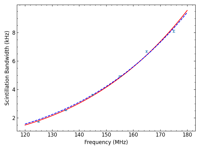
Figure 1: Measured scintillation bandwidth $\Delta\nu_{\rm{d}}$ vs frequency for LOFAR HBA observations. The fitted (red) line has an exponent 4.6. The blue dashed line has the Kolmogorov exponent $\alpha=4.4$.

3.2 DM Analysis

Our DM analysis is based on HBA data from five German stations of the International LOFAR Telescope (ILT, van Haarlem et al., 2013), taken between 05 March 2013 and 21 September 2021. For the monitoring observations used in this work, the five LOFAR stations of the German LOng Wavelength (GLOW) consortium, located in Effelsberg (telescope identifier DE601, 75 observations), Tautenburg (DE603, 288 observations), Potsdam-Bornim (DE604, 12 observations), Jülich (DE605, 13 observations) and Norderstedt (DE609, 82 observations), are used as individual stand-alone telescopes, not connected to the ILT network, as described in detail by Donner et al. (2019). In the end, the time and frequency resolution of GLOW data are $\sim$10 s and $\sim$0.195 MHz, respectively, with 1024 pulse phase bins. The details of our DM determination are identical to the description by Tiburzi et al. (2021).

The ecliptic latitude of PSR J0826+2637 is only 7.24^∘ so the solar wind contribution to DM is significant for several months of the year. We use the techniques of Tiburzi et al. (2021) to estimate the ISM component of DM, then we remove all observations with a solar elongation $<50^{\circ}$ and we remove outliers with respect to the ISM component greater than 3 sigma. The results are shown as blue error bars in Figure 2. The times of the observations used for our scattering study are shown as vertical dashed lines. They are taken at solar elongation of $\sim 40^{\circ}$ at which a solar wind contribution is possible. We augmented the plot with red error bars for observations between 40^∘ and 50^∘ and it is clear that there are no significant DM variations, as measured at 150 MHz, around these times. However the observations occur during a significant positive DM gradient which will shift the lines of sight at LOFAR and NenuFAR differentially.

The DM is a column density so it is directly proportional to the additional phase due to the plasma on the line of sight. The constant of proportionality $C_{dm2\phi}=0.830\pi 10^{10}/\nu_{\rm MHz}\rm{rad}\,\rm{pc}\,\rm{cm}^{3}$.

The DM gradient, $\sim$5.8333 $\times 10^{-5}$ pc cm^-3/AU, can be converted to a phase gradient and the corresponding angular shift $\theta_{\rm g}=\nabla\phi/k$ calculated. We find that $\theta_{\rm g}=0.28\,\theta_{\rm 0}$ at the highest NenuFAR frequency of 46.6 MHz. This shift is in the direction of the velocity so the observations of $\tau_{\rm sc}$ are in a region of somewhat higher DM. However the scattering disc for the LOFAR HBA observations remains within the scattering disc for NenuFAR observations. Note that $\theta_{\rm g}\propto\lambda^{2}$ whereas $\theta_{o}\propto\lambda^{2.2}$ so the relative importance of $\theta_{\rm g}$ decreases slowly with $\lambda$.

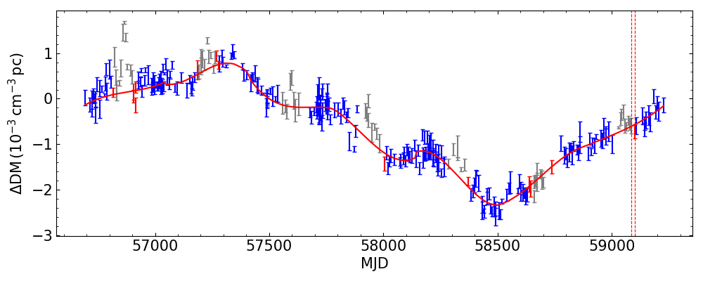
Figure 2: $\rm{DM}$ time series in the direction of PSR J0826+2637 measured by LOFAR. A DM baseline of 19.47921 $\rm{cm^{-3}\,pc}$ is subtracted. Observations closer than 40^∘ from the Sun are gray error bars. Observations outside of 50^∘ are blue error bars and those between 40^∘ and 50^∘ are red error bars. The ISM contribution estimated using the techniques in Tiburzi et al. 2021 is shown in red. Two dashed lines indicate the epochs MJD 59087 and MJD 59101, respectively.

3.3 Pulse Profile Analysis

PSR J0826+2637 is part of a long-term monitoring programme with NenuFAR. The NenuFAR data used for pulse profile studies have 2048 pulse phase bins. To correct dispersion in the narrow spectral channels, coherent dedispersion was applied in real time with the Low frequency Ultimate Pulsar Processing Instrument (LUPPI) described by Bondonneau et al. (2021). Due to the lack of a well-tested calibration scheme for NenuFAR data, we focus on the uncalibrated total-intensity data.

To model the pulse profiles, the fitting model reported in Krishnakumar et al. (2015) is used. With the assumption of a simple thin screen model dominating the scattering (e.g., Williamson, 1972), the observed pulse profile can be expressed as a convolution of the frequency-dependent intrinsic pulse shape $P_{i}(t,\nu)$ with the PBF(t), i.e. $\rm{P(t)=P_{i}(t,\nu)\ast PBF(t)}$, where $\ast$ denotes convolution. The pulse broadening by DM is negligible since coherent dedispersion has been applied.

PSR J0826+2637 is known to have a three-component pulse profile consisting of main pulse, postcursor and an interpulse and exhibits a bright (B-mode) and a quiet emission mode (Q-mode) in LOFAR observations (Sobey et al., 2015). In our NenuFAR observations, no nulling and Q-mode are detected and the postcursor and interpulse components are hidden in the noise (see Fig. 3). Thus, in this work, a single Gaussian profile model is used as the intrinsic pulse profile.

An illustration to demonstrate the procedure used to estimate $\tau_{\rm{sc}}$ is given in Figure 3, which shows an example of PSR J0826+2637 at $33\pm 1\,$MHz. Afterwards, we estimate $\alpha$ from $\tau_{\rm{sc}}$ derived from multiple sub-bands across our data (see Figure 4). We note that some $\tau_{\rm{sc}}$ values are excluded from the subsequent analysis (specifically, for deriving the power-law index $\alpha$), in particular when $\tau_{\rm{sc}}$ is nearly equal to or smaller than the pulse width at the higher frequency bands. It is clear that the best power-law exponent is near 2.7$\pm$0.1, but that a power-law fit is marginal because neither extreme frequency is well matched. The scattering time observations are definitely inconsistent with the assumption of a thin screen and a homogeneous power-law scattering medium.

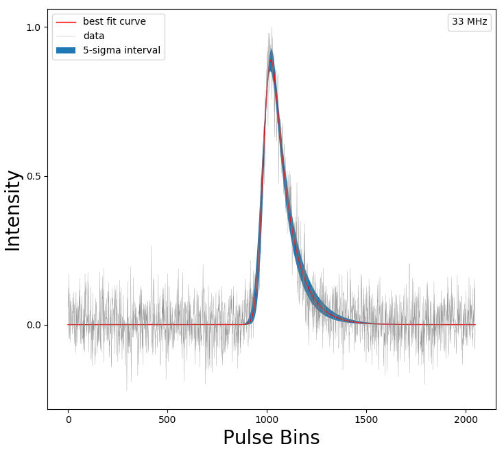
Figure 3: Average total-intensity NenuFAR pulse profile (in grey) of PSR J0826+2637 at 33$\pm$1 MHz at epoch MJD 59087. The time and frequency resolution of NenuFAR data are $\sim$10 s and $\sim$0.195 MHz, respectively. The red curve represents the best-fitting model and the blue band is the uncertainty.

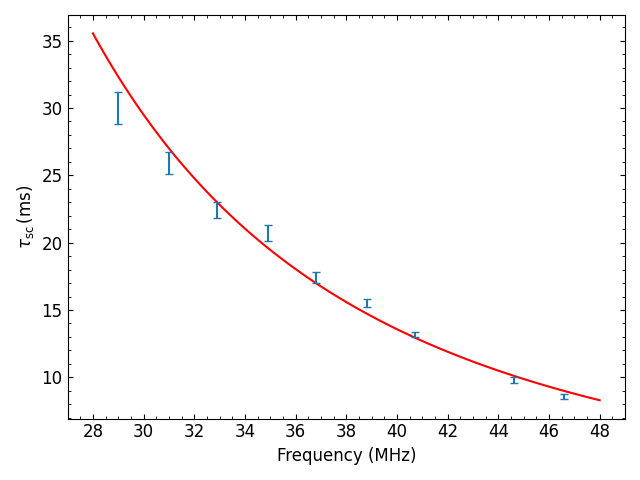
Figure 4: The pulse broadening time $\rm{\tau_{sc}}$ versus observing frequency for PSR J0826+2637. The red line has an exponent $\alpha=-2.7$.

3.4 Scintillation Arc

Intensity scintillation can be observed to form a dynamic spectrum of intensity as a function of frequency and time $I(\nu,t)$. The 2D Fourier transform of this dynamic spectrum $S_{\rm sec}(\tau,f_{\rm{d}})=F_{2}(I(\nu,t))$, is the “secondary spectrum”. The dynamic spectrum is caused by interference between components of the scattered angular spectrum of plane waves. Those scattered plane waves each have a well-defined delay and Doppler shift with respect to an unscattered plane wave. The axes of $S_{\rm sec}$ are the differential delay $\tau_{\rm d}$ and differential Doppler shift $f_{\rm{d}}$, so $S_{\rm sec}$ is a distribution of the received angular spectrum in differential delay and differential Doppler.

Parabolic arcs can be observed in the $S_{\rm sec}$ only when the scattering is dominated by a compact region somewhere along the line of sight (Walker et al., 2004; Cordes et al., 2006). In this case $\tau_{\rm d}$ and $f_{\rm d}$ are uniquely defined by the scattering angles of the two interfering waves $\boldsymbol{\theta_{\rm 1}}$ and $\boldsymbol{\theta_{\rm 2}}$ giving

$$\tau_{\rm d} =D\,((1-s)/2cs)\,(\boldsymbol{\theta_{\rm 1}}^{2}-\boldsymbol{\theta_{\rm 2}}^{2})\,\,\,\rm{and}$$ (3)

$$f_{\rm d} =(1/\lambda s)\,(\boldsymbol{\theta_{\rm 1}}-\boldsymbol{\theta_{\rm 2}})\cdot\boldsymbol{{V}_{\rm{eff}}}\,\,\,\rm{where}$$ (4)

$$\boldsymbol{V_{\rm{eff}}} =(1-s)\boldsymbol{V_{\rm{p}}}+s\boldsymbol{V_{\rm{E}}}-\boldsymbol{{V}_{\rm{ISM}}}(s).$$ (5)

Here s is the fractional distance from the pulsar to the scattering screen. The pulsar velocity is 272 kms^-1 (Deller et al., 2019) so, to first order, the contributions of $V_{\rm E}$ and $V_{\rm ISM}$ can be ignored.

In PSR J0826+2637 we see a forward arc with its apex near the origin of $S_{\rm sec}$. Such arcs are caused by highly scattered plane waves interfering with waves closer to the origin of the angular spectrum. The “boundary” arc is defined by the maximum Doppler for a given delay, so $\boldsymbol{\theta_{\rm 2}}\rightarrow 0$ and $\boldsymbol{\theta_{\rm 1}}$ is parallel to $\boldsymbol{{V}_{\rm eff}}$. It is very useful to normalize $\tau_{\rm d}$ by the values they would have if $\theta_{\rm 1}=\theta_{\rm o}$, i.e. $\tau_{\rm sc}$ and $2\pi s/\tau_{\rm o}$. This which gives $\tau_{\rm dn}=(\theta_{\rm 1}/\theta_{\rm o})^{2}$ and $f_{\rm dn}$ = $\theta_{\rm 1}/\theta_{\rm o}$. The arc is then given by $\tau_{\rm dn}=f_{\rm dn}^{2}$ so the normalized arc curvature is unity.

When a phase gradient in the direction of the velocity is present in the scattering medium the entire angular spectrum is shifted by an angle $\theta_{\rm g}$ (Cordes et al., 2006). This does not alter the Doppler $f_{\rm dn}$ but it changes the normalized delay to

$$\tau_{\rm dn} =f_{\rm dn}^{2}+2(\theta_{\rm g}/\theta_{\rm o})f_{\rm dn}\,\,\,{\rm and}$$ (6)

$$\tau_{\rm d} =\eta f_{\rm d}^{2}+\gamma f_{\rm d}.$$ (7)

The parabolic arc still passes through the origin but its apex is shifted to $f_{\rm dn}=-\theta_{\rm g}/\theta_{\rm o}$. This factor increases from 0.28 at 46.6 MHz, to 0.354 at 150 MHz.

The secondary spectrum observed on MJD 59101 is shown in Figure 5 in observed units $\tau_{\rm d}$ and $f_{\rm d}$. The amplitude is $\log_{10}(S_{\rm sec})$. The arc is not sharply defined but $\eta=1.7s^{3}$ and $\gamma=-0.00441s^{2}$ can be estimated. This provides an estimate of s = 0.56. If the phase gradient were not included one would estimate s = 0.66, a 20% difference.

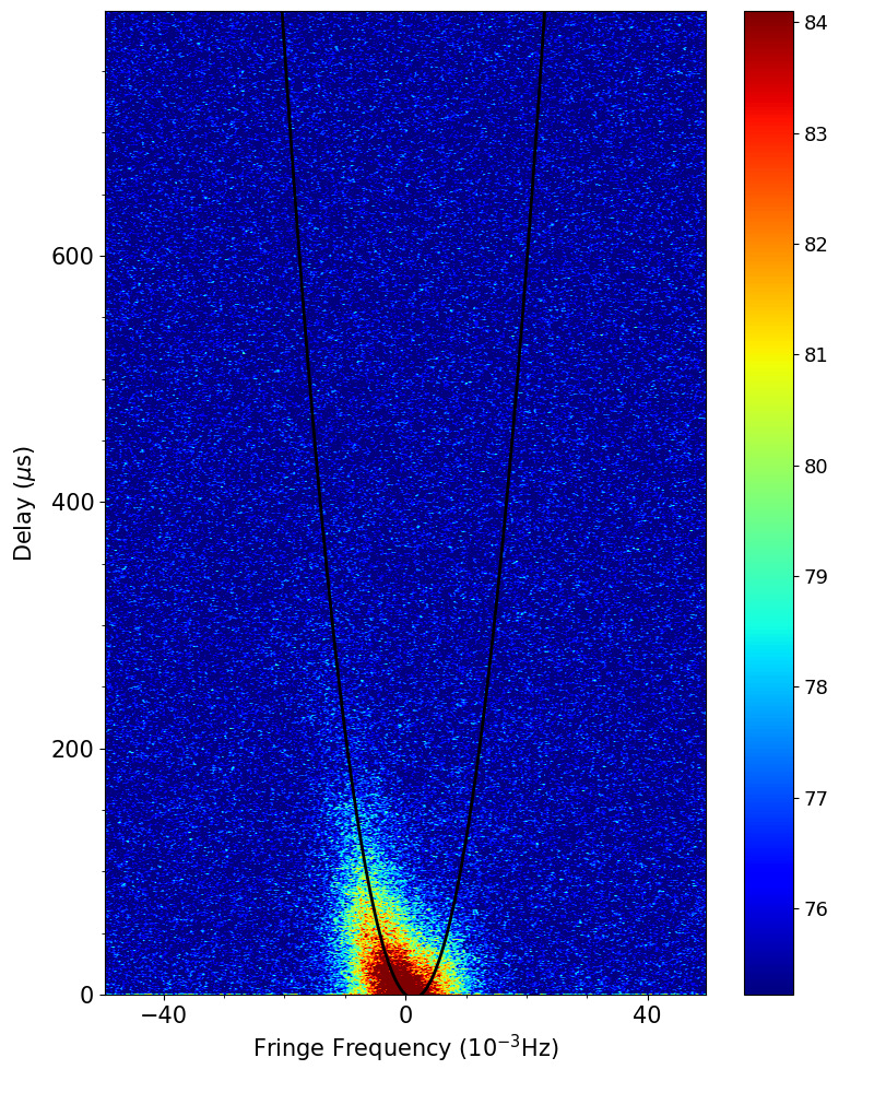
Figure 5: Observed secondary spectrum of PSR J0826+2637 with LOFAR in the frequency range 145 – 155 MHz at MJD 59101. The asymmetric parabola corrects for the phase gradient and implies s=0.56.

4 Analysis and results

To resolve the inconsistency between the scintillation bandwidth and scattering time observations, it is helpful to put both in context with the larger scale $\Delta\rm{DM}(t)$ observations. This could be done with the power spectra, but it is more directly done using the structure function of DM. We first convert $\Delta\rm{DM}(t)$ to $\Delta\rm{DM}({r})$ using $\boldsymbol{r}=\boldsymbol{V_{\rm eff}}\,t$. The structure function of DM is $D_{\rm DM}(s)=\langle(\rm{DM}(r)-\rm{DM}(r+s))^{2}\rangle$. It can be directly compared with the $\tau_{\rm sc}\,{\rm and}\,\Delta\nu_{\rm d}$ measurements each of which provides a measurement of $s_{\rm 0}$. By definition, $D_{\phi}(s_{0})=1$. Since $\phi$ is directly related to DM this provides a measurement of $D_{\rm DM}(s_{0})$ at a much smaller scale. The phase $\phi$ equals $C_{dm2\phi}\,\rm{DM}$ where the constant $C_{dm2\phi}=0.830\,\pi\,10^{10}/\,\nu_{\rm MHz}$.

So $D_{\rm DM}=D_{\phi}\,C_{dm2\phi}^{-2}$. In this way a sample of $D_{\phi}(s_{0})=1$ obtained from a bandwidth or a scattering time measurement, can be converted to $D_{\rm DM}(s_{0})=C_{dm2\phi}^{-2}$. The value of $s_{0}$ can be obtained from $\theta_{0}=(\tau_{\rm sc}2c/V_{\rm eff})^{0.5}$ and $s_{0}=1/k\theta_{0}$.

The structure function $D_{\rm DM}$ was obtained directly from the definition by calculating all the squared differences and binning them to obtain an average. We did not weight the squared differences by their white noise error bars because the white noise is not the primary source of estimation error. That is the finite number of independent estimates in that average. The estimate of $D_{\rm DM}$ directly from the $\Delta\rm{DM}(s=V_{\rm eff}t)$ time series is plotted in Figure 6, with estimates from the HBA scintillation bandwidth measurements and the samples of $\tau_{\rm sc}$ from NenuFAR.

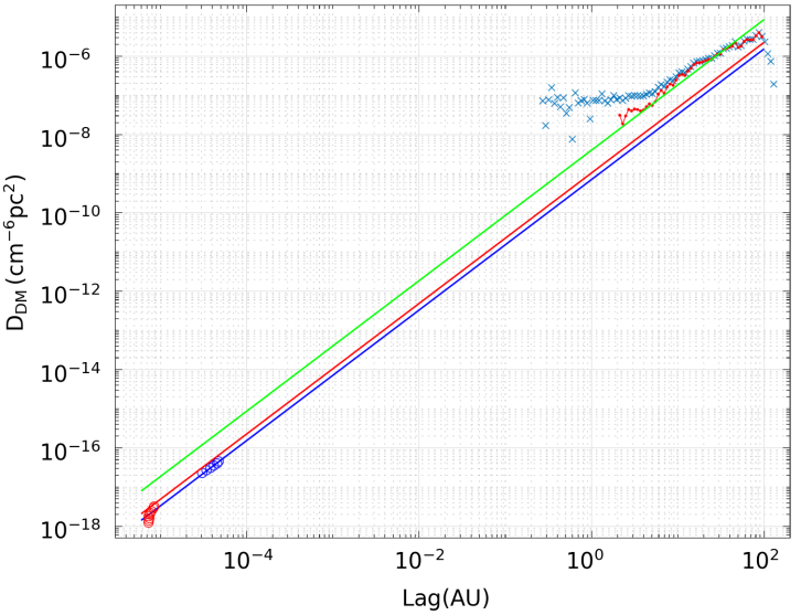
Figure 6: Structure function $D_{\rm DM}(s=V_{\rm eff}t)$. The blue x symbols are the raw estimates. The red filled circles have had the white noise contribution subtracted. The white noise subtraction is not reliable for $s<2$ AU and $D_{\rm DM}$ is heavily biased by the limited data length for $s>100$ AU, so the red line is limited to $2<s<100$ AU. The blue circles are from the LOFAR HBA measurements of $\Delta\nu_{d}$. The red squares are from the NenuFAR $\tau_{\rm sc}$ values. The straight red line is the best Kolmogorov model which fits the NenuFAR data. The straight blue line is the equivalent for the LOFAR HBA data. The straight green line best fits the observed $D_{\rm DM}$.

One can see that the Kolmogorov extrapolation of the large scales exceeds the NenuFAR 46.6 MHz estimate by a factor of 3.8. The LOFAR HBA estimates, which by themselves have the Kolmogorov exponent, fall below the large-scale extrapolation by a factor of 5.6. There are two points to be explained: the scattering observations come from a weaker scattering region than the average of the $\Delta\rm{DM}$ observations; and the NenuFAR observations cannot come from a thin homogeneous scattering screen. The scattering screen must be thin because an arc is observed, so it cannot be homogeneous. This inhomogeneity can also explain why the HBA observations come from a weaker scattering region.

A simple model of an inhomogeneity that would explain our observations, is that the scattering region has a finite extent of $\sim$40 AU. At frequencies of $\geq 46.6$ MHz the scattering disc $\theta_{0}D_{\rm eff}$ is smaller than 40 AU so the scattering appears homogeneous. However at lower frequencies the scattering disc exceeds 40 AU. This limits the angular spectrum received by the observer and thus $\tau_{\rm sc}$ fails to increase as expected. Inhomogeneity also explains why the scattering estimates of $D_{\rm DM}(s_{0})$ are lower than the large scale average. Indeed the direct observations of $\Delta\rm{DM}(t)$ indicate that DM during the observations is lower than the average but increasing. The refractive gradient will cause the NenuFAR observations to be observed later than the LOFAR HBA observations and thus in a region of stronger scattering. The displacement of the scattering disc is only about 28% of its width at 46.6 MHz, but the width of the scattering disc at 150 MHz is very much smaller. Its area is < 1% of the area of the NenuFAR scattering disc, so the reduced scattering at 150 MHz could be due to a density variation on a scale of $\sim$ 2AU which would be invisible to the low frequencies.

4.1 Finite Screen Model

The angular spectrum scattered by the turbulent plasma is the same as the angular spectrum seen by the observer if the scattering medium is homogeneous. However if the scattering plasma does not fully occupy the scattering disc then the observed angular spectrum will be smaller than the scattered angular spectrum. This will increase $s_{0}\,{\rm and}\,\Delta\nu_{\rm d}$ but decrease $\tau_{\rm sc}$. As the size of the scattering disc increases at lower frequencies ($\propto\nu^{-2.2}$ for a Kolmogorov spectrum) the effect becomes more pronounced at lower frequencies.

Clearly the behavior of, e.g. $\tau_{\rm sc}$, depends on the distribution of the plasma within the scattering disc. Here we choose the simple model of a gaussian plasma distribution $\rm{B(\theta)_{\rm{cloud}}=exp(-(\theta/\theta_{cloud})^{2})}$ centered in a gaussian scattering disc $\rm{B(\theta)_{\rm{scat}}=exp(-(\theta/\theta_{scat})^{2})}$. The observer will then see

$$B(\theta)_{\rm{obs}}=\rm{exp}(-[(\theta/\theta_{\rm{scat}})^{2}+(\theta/\theta_{\rm{cloud}})^{2}])=\rm{exp}(-(\theta/\theta_{\rm{tot}})^{2})$$ (8)

where $\theta_{\rm{tot}}^{2}=(1/\theta_{\rm{scat}}^{2}+1/\theta_{\rm{cloud}}^{2})^{-1}$. In terms of measurable parameters, $\tau_{\rm sc}\,{\rm and}\,\Delta\nu_{\rm{d}}$, $\theta_{0}$ is replaced by $\theta_{\rm tot}$.

The model is compared with the data in Figure 7. The data points marked with blue squares are the bandwidth calculated from the measured $\tau_{\rm sc}$ at NenuFar. The solid red curve that passes through the NenuFAR observations is the finite screen model adjusted to best match them. It has a cloud size that matches the scattering disc at 33 MHz, i.e. $\sim\,40\,\rm{AU}$. The $D_{\rm DM}$ of this model is shown as a straight red line on Figure 6. It lies a factor of 3.8 below that computed directly from the $\Delta DM$ observations in the range 2 to 100 AU. The bandwidth computed for this model with a very large blob size is shown as a solid green line. The LOFAR HBA bandwidth measurements are shown as blue + symbols. They lie a factor of 1.5 above the green line (i.e. lower in turbulence level).

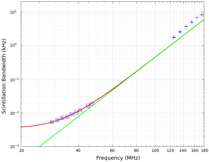
Figure 7: The scintillation bandwidth $\Delta\nu_{\rm{d}}$ as a function of observing frequency. The blue squares are calculated from the observed $\tau_{\rm sc}$ at NenuFAR. The solid red curve that passes through the NenuFAR observations is the finite screen model adjusted to best match them. It has a cloud size that matches the scattering disc at 33 MHz, i.e. $\sim\,40\,$AU. The bandwidth computed for this model with a very large blob size is shown as a solid green line.The LOFAR HBA measurements of scintillation bandwidth are shown as blue + symbols.

4.2 Summary

The parabolic arc measurements show the scattering screen is relatively thin and located roughly midway between the pulsar and the Earth. The $\Delta\rm{DM}(t)$ observations show that the fluctuations, averaged over a 100 AU trajectory are Kolmogorov between scales of 2 AU and 100 AU. The structure function of DM, $D_{\rm{DM}}$, can be extrapolated down to scales of 5 $\times$ $10^{-6}$ AU where it exceeds the estimated $D_{\rm{DM}}$ from the NenuFAR observations by a factor of 3.8 and that estimated from the LOFAR HBA observations by a factor of 5.7.

The LOFAR HBA estimates are consistent with a Kolmogorov exponent but at a lower level. The lower frequency NenuFAR observations cannot be explained by a thin scattering screen with homogeneous power-law spatial spectrum, but they can be modeled using a finite scattering screen with a spatial scale of $\sim$ 40  AU. Thus all observations are consistent with a Kolmogorov scattering medium that is not stationary in variance on scales $\geq$40 AU.

4.3 Other Observations

The frequency-dependence of $\tau_{\rm sc}$ and $\Delta\nu_{\rm d}$ for PSR J0826+2637 has previously been studied: Bansal et al. (2019) found that the median value of $\alpha$ is 1.55$\pm$0.09 based on their long-term monitoring of $\tau_{\rm sc}$ with the Long Wavelength Array (LWA) at frequencies ranging between 44 and 75 MHz; Krishnakumar et al. (2019) reported a value of 2.4$\pm$0.1 for $\alpha$ based on combined $\tau_{\rm sc}$ data from the LWA and the Ooty Radio Telescope in the frequency range of 32–62 MHz; Daszuta et al. (2013) found $\alpha$ = 3.94$\pm$0.36 from the measured $\Delta{\nu_{\rm{d}}}$ over a wide frequency band (300-1700 MHz) at different epochs; and in Paper I we reported $\alpha$ = 4.12$\pm$0.16 from LOFAR HBA measurements of $\Delta{\nu_{\rm{d}}}$ at 150 MHz. Our analysis of $\tau_{\rm sc}$ gives $\alpha=2.71\pm 0.11$ (see Table 1). In contrast, our analysis of LOFAR $\Delta\nu_{\rm d}$ taken on MJD 58820 results in $\alpha=4.58\pm 0.16$. It is clear that the low frequency observations are all affected by inhomogeneity. It is also clear that to make an accurate estimate of the spectral exponent one needs a longer spatial baseline. Comparison of scattering observations and DM observations provides a much more precise technique.

4.4 Other Sources of Error

There are other possibilities summarized below that could bias estimates of the pulse broadening delay $\tau_{\rm{sc}}$:

1. The pulsar radio emission mechanism. There are two components in the fitted model $P(t)$: $\tau_{\rm sc}$ and the intrinsic pulse profile. The width of the intrinsic pulse profile is frequency-dependent, which is not fully understood yet (Lorimer & Kramer, 2012) and could affect the above measurements.

2. Pulse profile with multiple components. The postcursor and interpulse components of PSR J0826+2637 are not distinguished in our NenuFAR data due to the limited S/N. This could disturb the fitting procedure. In order to resolve postcursor and interpulse components of PSR J0826+2637 with NenuFAR, the data with longer observation length are required. Moreover, other fitting procedures; e.g., the forward fitting method of Geyer & Karastergiou (2016), and the deconvolution method by Bhat et al. (2003) could provide more insight into pulsar profile analysis, particularly for pulsars with multi-component pulse profiles.

5 Conclusion

We find that near-simultaneous observations of PSR J0826+2637 from NenuFAR at 28 to 48 MHz and LOFAR from 120 to 180 MHz are not consistent with a homogeneous power-law scattering medium. The LOFAR measurements are internally consistent with a homogeneous Kolmogorov medium over a scattering disc of 2.5 AU in radius. The NenuFAR observations are consistent with a Kolmogorov scattering blob of $\sim$ 40 AU in radius. However the scattering disc of the NenuFAR observations below 46 MHz is larger than 40 AU and this limits the scattering time at lower frequencies.

The non-standard frequency-dependence of the scattering properties presented here, could be a common feature particularly at very low observing frequencies, since similar abrupt inhomogeneities on AU scales have regularly been reported in observations of scintillation arcs (Stinebring et al., 2022). Further observations including other low frequency facilities, e.g. the Long Wavelength Array (Taylor et al., 2012) the Murchison Widefield Array (Tingay et al., 2013) and the Ukrainian T-shaped Radio telescope (Zakharenko et al., 2013) could significantly improve the models of the physical size of scattering screens in the near future.

Data Availability

The data underlying this article will be shared on reasonable request to the corresponding author.

References

- Armstrong et al. (1995) Armstrong J. W., Rickett B. J., Spangler S. R., 1995, ApJ, 443, 209
- Bansal et al. (2019) Bansal K., Taylor G. B., Stovall K., Dowell J., 2019, ApJ, 875, 146
- Bhat et al. (2003) Bhat N. D. R., Cordes J. M., Chatterjee S., 2003, ApJ, 584, 782
- Bondonneau et al. (2020) Bondonneau L., Grießmeier J. M., Theureau G., Bilous A. V., Kondratiev V. I., Serylak M., Keith M. J., Lyne A. G., 2020, A&A, 635, A76
- Bondonneau et al. (2021) Bondonneau L., et al., 2021, A&A, 652, A34
- Cordes & Lazio (2001) Cordes J. M., Lazio T. J. W., 2001, ApJ, 549, 997
- Cordes & Rickett (1998) Cordes J. M., Rickett B. J., 1998, ApJ, 507, 846
- Cordes et al. (2006) Cordes J. M., Rickett B. J., Stinebring D. R., Coles W. A., 2006, ApJ, 637, 346
- Daszuta et al. (2013) Daszuta M., Lewandowski W., Kijak J., 2013, MNRAS, 436, 2492
- Deller et al. (2019) Deller A. T., et al., 2019, ApJ, 875, 100
- Donner et al. (2019) Donner J. Y., et al., 2019, A&A, 624, A22
- Geyer & Karastergiou (2016) Geyer M., Karastergiou A., 2016, MNRAS, 462, 2587
- Geyer et al. (2017) Geyer M., et al., 2017, MNRAS, 470, 2659
- Hotan et al. (2004) Hotan A. W., van Straten W., Manchester R. N., 2004, PASA, 21, 302
- Krishnakumar et al. (2015) Krishnakumar M. A., Mitra D., Naidu A., Joshi B. C., Manoharan P. K., 2015, ApJ, 804, 23
- Krishnakumar et al. (2019) Krishnakumar M. A., Maan Y., Joshi B. C., Manoharan P. K., 2019, ApJ, 878, 130
- Lazarus et al. (2016) Lazarus P., Karuppusamy R., Graikou E., Caballero R. N., Champion D. J., Lee K. J., Verbiest J. P. W., Kramer M., 2016, MNRAS, 458, 868
- Liu et al. (2022) Liu Y., et al., 2022, A&A, 664, A116
- Lorimer & Kramer (2012) Lorimer D. R., Kramer M., 2012, Handbook of Pulsar Astronomy (Cambridge: Cambridge University Press)
- Rickett (1977) Rickett B. J., 1977, ARA&A, 15, 479
- Rickett (1990) Rickett B. J., 1990, ARA&A, 28, 561
- Romani et al. (1986) Romani R. W., Narayan R., Blandford R., 1986, MNRAS, 220, 19
- Sobey et al. (2015) Sobey C., et al., 2015, MNRAS, 451, 2493
- Stinebring et al. (2022) Stinebring D. R., et al., 2022, ApJ, 941, 34
- Taylor et al. (2012) Taylor G. B., et al., 2012, Journal of Astronomical Instrumentation, 1, 1250004
- Tiburzi et al. (2021) Tiburzi C., et al., 2021, A&A, 647, A84
- Tingay et al. (2013) Tingay S. J., et al., 2013, Publ. Astron. Soc. Australia, 30, e007
- Verbiest & Shaifullah (2018) Verbiest J. P. W., Shaifullah G. M., 2018, Classical and Quantum Gravity, 35, 133001
- Verbiest et al. (2021) Verbiest J. P. W., Osłowski S., Burke-Spolaor S., 2021, in , Handbook of Gravitational Wave Astronomy. p. 4, doi:10.1007/978-981-15-4702-7_4-1
- Walker et al. (2004) Walker M. A., Melrose D. B., Stinebring D. R., Zhang C. M., 2004, MNRAS, 354, 43
- Williamson (1972) Williamson I. P., 1972, MNRAS, 157, 55+
- Wu et al. (2022) Wu Z., et al., 2022, A&A, 663, A116
- Zakharenko et al. (2013) Zakharenko V. V., et al., 2013, MNRAS, 431, 3624
- Zarka et al. (2020) Zarka P., et al., 2020, in URSI GASS 2020, Session J01 New Telescopes on the Frontier.
- van Haarlem et al. (2013) van Haarlem M. P., et al., 2013, A&A, 556, A2
- van Straten & Bailes (2011) van Straten W., Bailes M., 2011, PASA, 28, 1
- van Straten et al. (2012) van Straten W., Demorest P., Osłowski S., 2012, Astronomical Research and Technology, 9, 237