A general class of linear unconditionally energy stable schemes for the gradient flows, II

Abstract

This paper continues to study linear and unconditionally modified-energy stable (abbreviated as SAV-GL) schemes for the gradient flows. The schemes are built on the SAV technique and the general linear time discretizations (GLTD) as well as the extrapolation for the nonlinear term. Different from [44], the GLTDs with three parameters discussed here are not necessarily algebraically stable. Some algebraic identities are derived by using the method of undetermined coefficients and further used to establish the modified-energy inequalities for the unconditional modified-energy stability of the semi-discrete-in-time SAV-GL schemes. It is worth emphasizing that those algebraic identities or energy inequalities are not necessarily unique for some choices of three parameters in the GLTDs. Numerical experiments on the Allen-Cahn, the Cahn-Hilliard and the phase field crystal models with the periodic boundary conditions are conducted to validate the unconditional modified-energy stability of the SAV-GL schemes, where the Fourier pseudo-spectral method is employed in space with the zero-padding to eliminate the aliasing error and the time stepsizes for ensuring the original-energy decay are estimated by using the stability regions of our SAV-GL schemes for the test equation. The resulting time stepsize constraints for the SAV-GL schemes are almost consistent with the numerical results on the above gradient flow models.

1 Introduction

Many practical problems could be modeled by the gradient flows, e.g., the interface dynamics [1, 57], the liquid crystallization [31, 32], the thin films [30, 46], the polymers [18, 19], and the the tumor growth [35, 49]. For a given free energy $\mathcal{E}(u)$, the gradient flow model can be given by

$$\frac{\partial u}{\partial t}=\mathcal{G}\frac{\delta\mathcal{E}}{\delta u},~{}~{}~{}~{}(\mbox{\boldmath\small$x$},t)\in\Omega\times(0,T],$$ (1.1)

supplemented with suitable initial and boundary conditions, where $\Omega\subset\mathbb{R}^{d},d=1,2,3$, $u=u(\mbox{\boldmath\small$x$},t)\in\mathbb{R}$, the operator $\mathcal{G}$ is negative, $\delta\mathcal{E}/\delta u$ denotes the variational derivative of the free energy functional $\mathcal{E}(u)$ with respect to the variable $u$, known as the chemical potential. Obviously, (1.1) implies that the free energy is monotonically non-increasing, that is,

$$\frac{d\mathcal{E}}{dt}=\left(\frac{\delta\mathcal{E}}{\delta u},\frac{\partial u}{\partial t}\right)=\left(\frac{\delta\mathcal{E}}{\delta u},\mathcal{G}\frac{\delta\mathcal{E}}{\delta u}\right)\leq 0,$$ (1.2)

and the triple $\left\{u,\mathcal{G},\mathcal{E}\right\}$ determines the gradient flow uniquely, where $(\cdot,\cdot)$ is the $L^{2}$ inner product defined by $(\phi,\psi)=\int_{\Omega}\phi\psi d\mbox{\boldmath\small$x$}$ for any $\phi,\psi\in L^{2}(\Omega)$. It is worth noting that (1.2) holds only for the boundary conditions such as periodic or homogeneous Neumann boundary conditions which can make the boundary integrals resulted from the integration by parts vanish.

In the last few decades, many high-order accurate and unconditionally energy stable schemes have been developed for various nonlinear gradient flow models. Those include, but are not limited to, the convex splitting method [16, 17, 39], the stabilization method [45, 37, 47], the Lagrange multiplier method [4, 23], the exponential time differencing method [48, 14], and more recently, the invariant energy quadratization method [51, 52, 53, 55], the scalar auxiliary variable (SAV) method [40, 41, 42] and its extensions, such as the exponential SAV [33, 34], the generalized SAV (G-SAV) [26, 27] and the SAV with relaxation [28], etc. Among those, the SAV approach and its variants become a particular powerful tool to construct modified-energy stable numerical schemes and has been successfully applied to many existing gradient flow models, see e.g. [3, 10, 11, 22, 25, 54, 56, 28, 58]. Its main idea is to reformulate the gradient flow model into an equivalent form with the help of some SAVs, and then to develop efficient numerical schemes by approximating the reformulated system instead of the original gradient flow model. Based on those SAV approaches, it is convenient to construct second- or higher-order unconditionally modified-energy stable schemes, and the derived schemes are easy to be implemented and only need to solve several linear equations at each time step if the nonlinear term is explicitly approximated by the extrapolation etc.

Recently, in [44], the authors studied a general class of linear unconditionally modified-energy stable schemes for the gradient flows. Those schemes (abbreviated as SAV-GL) are built on the (original) SAV approach and the general linear time discretizations (GLTD) as well as the linearization based on the extrapolation for the nonlinear term. The proof of their unconditional modified-energy stability uses the algebraical stability of the GLTDs. This paper continues to study the SAV-GL schemes for the gradient flows, and will mainly addresses three issues: 1) How the modified-energy inequality of the SAV-GL is derived if the GLTDs are not necessarily algebraically stable? 2) Whether the modified-energy inequality is unique? 3) How a suitable time stepsize is chosen to ensure the original-energy decay because the unconditional modified-energy stability does not imply the unconditional original-energy stability generally? The main contributions are as follows: Different from [44], the GLTDs with three parameters discussed here are not necessarily algebraically stable. Some algebraic identities are first derived by using the method of undetermined coefficients and are then used to establish the modified-energy inequalities for the unconditional modified-energy stability of the semi-discrete-in-time SAV-GL schemes. Those algebraic identities or energy inequalities are not necessarily unique for some choices of three parameters in the GLTDs. In order to validate the energy stabilities of the SAV-GL schemes, numerical experiments on the Allen-Cahn, the Cahn-Hilliard and the phase field crystal models with the periodic boundary conditions are conducted, the Fourier pseudo-spectral method is employed in space with the zero-padding to eliminate the aliasing error, and the restrictions on the time stepsize for preserving the original-energy stability are estimated by studying the stability regions of our SAV-GL schemes for the test equation.

The rest of this paper is organized as follows. Section 2 presents our new linear unconditionally modified-energy stable schemes (still abbreviated as SAV-GL) for the gradient flows, built on the GLTDs with three parameters and the SAV approach. Here the GLTDs are not necessarily algebraically stable. Some algebraic identities are derived for the modified-energy inequality of the SAV-GL, and they may not be necessarily unique for some choices of three parameters in the GLTDs. Section 3 conducts some numerical experiments to validate the theoretical analysis of the SAV-GL schemes in comparison to another SAV-GL schemes built on the generalized SAV [26, 27], where the Allen-Cahn, Cahn-Hilliard and phase field crystal models with the periodic boundary conditions are considered, the Fourier pseudo-spectral method is employed in space with the de-aliasing by zero-padding, and the time stepsizes for ensuring the original-energy decay are also estimated by the stability regions of our SAV-GL schemes for the test equation. Some concluding remarks are given in Section 4.

2 SAV-GL schemes for the gradient flows

This section studies the general linear time discretizations (GLTDs) with three parameters, which are not necessarily algebraically stable, and develops the semi-discrete-in-time linear SAV schemes (still abbreviated as SAV-GL) for the gradient flow model (1.1) with the help of the original SAV approach [40, 41, 42]. Their unconditional modified-energy stability will be derived with some algebraic identities, established by using the method of undetermined coefficients.

Assume that the free energy $\mathcal{E}(u)$ contains some quadratic terms such as

$$\mathcal{E}(u)=\frac{1}{2}(\mathcal{L}u,u)+\mathcal{E}_{1}(u),$$ (2.1)

where $\mathcal{L}$ is a linear, positive and self-adjoint operator, and $\mathcal{E}_{1}(u)$ denotes other nonlinear parts. Following the SAV approach [40, 41, 42], introduce the SAV $z(t):=\sqrt{\mathcal{E}_{1}(u)+C_{0}}$ with $C_{0}$ being a positive constant so that $z$ is real-valued, and then to rewrite the gradient flow model (1.1) as

$$\begin{aligned} \frac{\partial u}{\partial t}&=\mathcal{G}\mu,~{}~{}\mu=\mathcal{L}u+zW(u),\\ \frac{dz}{dt}&=\frac{1}{2}\left(W(u),\frac{\partial u}{\partial t}\right),~{}~{}~{}\ W(u):=\frac{1}{z(t)}\frac{\delta\mathcal{E}_{1}}{\delta u},\end{aligned}$$ (2.2)

supplemented with suitable initial and boundary conditions. Based on (2.2), one can construct the SAV schemes for the gradient flow model (1.1). It is easy to check that the reformulated system (2.2) satisfies the energy dissipation law

$$\frac{d\mathcal{F}}{dt}(u)=\left(\mathcal{L}u,\frac{\partial u}{\partial t}\right)+2z\frac{dz}{dt}=\left(\mathcal{L}u+zW(u),\frac{\partial u}{\partial t}\right)=\left(\mathcal{G}\mu,\mu\right)\leq 0,$$

where the reformulated free energy $\mathcal{F}(u)=\frac{1}{2}(\mathcal{L}u,u)+z^{2}-C_{0}$ is the same as the original $\mathcal{E}(u)$.

Let $\tau$ be a given time stepsize, $t_{n}=n\tau$ for $n\geq 0$ and $\chi^{n}$ denote an approximation to the generic variable $\chi$ at $t_{n}$. Approximate the variables $\chi$ and $\frac{\partial\chi}{\partial t}$ at $t_{n+\kappa}\!=\!t_{n}+\kappa\tau$ as follows

$$\frac{\partial\chi}{\partial t}\Big{|}^{n+\kappa}\!\approx\!\frac{1}{\tau({1\!-\!\alpha_{0}})}\!{\left[\chi^{n+1}\!-\!(1\!+\!\alpha_{0})\chi^{n}\!+\!{\alpha_{0}}\chi^{n-1}\right]}\!,$$ (2.3)

$$\chi^{n+\kappa}\!=\!\frac{1}{1\!-\!\alpha_{0}}\left(\beta_{2}\chi^{n+1}\!+\!{\beta_{1}}\chi^{n}\!+\!{\beta_{0}}\chi^{n-1}\right),$$ (2.4)

$$\bar{\chi}^{n+\kappa}=\left(1\!+\!\kappa\right)\chi^{n}-\kappa\chi^{n-1},$$ (2.5)

where $\alpha_{0}\neq 1,\beta_{2}\neq 0$ and $\beta_{0}$ are three free parameters, $\kappa=\frac{\beta_{2}-\beta_{0}}{1-\alpha_{0}}$, $\beta_{1}=1-\alpha_{0}-\beta_{0}-\beta_{2}$, and $\chi^{n+\kappa}$ (resp. $\bar{\chi}^{n+\kappa}$) denotes an implicit (resp. explicit) approximation to $\chi(t_{n+\kappa})$, so that (2.3)-(2.5) can provide at least first-order accurate time discretizations.

Lemma 2.1.

The fully implicit time discretizations based on (2.3)-(2.4) are $A-$stable (but are not necessarily algebraically stable) if

$$-1\leq\alpha_{0}<1,~{}~{}~{}\beta_{2}>0,~{}~{}~{}|\beta_{0}|\leq\beta_{2},~{}~{}~{}1-\alpha_{0}-2\beta_{0}-2\beta_{2}\leq 0.$$ (2.6)

Specially, (i) when $\alpha_{0}=\beta_{0}=0$, the time discretizations based on (2.3)-(2.4) are one-step and $A-$stable for any $\beta_{2}\geq\frac{1}{2}$; (ii) when $\beta_{2}=\frac{1+\alpha_{0}}{2}+\beta_{0}$ and $|\alpha_{0}|+|\beta_{0}|\neq 0$ (i.e. $\alpha_{0}$ and $\beta_{0}$ are not zero simultaneously), the time discretizations based on (2.3)-(2.4) are two-step and second-order accurate, which are $A-$stable for any $-1\leq\alpha_{0}<1$ and $2\beta_{0}+\alpha_{0}\geq 0$; and (iii) when $\beta_{2}\neq\frac{1+\alpha_{0}}{2}+\beta_{0}$ and $|\alpha_{0}|+|\beta_{0}|\neq 0$, the time discretizations based on (2.3)-(2.4) are two-step and first-order accurate, which are $A-$stable under (2.6).

The proof of Lemma 2.1 is given in A.

Assume that $(u^{n-1},z^{n})$ and $(u^{n},z^{n})$ are given. Applying (2.3)-(2.5) to the reformulated system (2.2) yields the following semi-discrete-in-time SAV-GL scheme

$$\begin{aligned} &\frac{1}{1\!-\!\alpha_{0}}u^{n+1}\!-\!\frac{1\!+\!\alpha_{0}}{1\!-\!\alpha_{0}}u^{n}\!+\!\frac{\alpha_{0}}{1\!-\!\alpha_{0}}u^{n-1}\!=\!\tau\mathcal{G}\mu^{n+\kappa},~{}~{}\mu^{n+\kappa}\!=\!\mathcal{L}u^{n+\kappa}\!+\!z^{n+\kappa}W(\bar{u}^{n+\kappa}),\\[3.0pt] &\frac{1}{1\!-\!\alpha_{0}}z^{n+1}\!-\!\frac{1\!+\!\alpha_{0}}{1\!-\!\alpha_{0}}z^{n}\!+\!\frac{\alpha_{0}}{1\!-\!\alpha_{0}}z^{n-1}\!=\!\frac{1}{2}\!\left(\!W(\bar{u}^{n+\kappa}),\frac{1}{1\!-\!\alpha_{0}}u^{n+1}\!-\!\frac{1\!+\!\alpha_{0}}{1\!-\!\alpha_{0}}u^{n}\!+\!\frac{\alpha_{0}}{1\!-\!\alpha_{0}}u^{n-1}\!\right)\!,\end{aligned}$$ (2.7)

where $u^{n+\kappa},z^{n+\kappa}$, and $\bar{u}^{n+\kappa}$ are given by (2.4) and (2.5), respectively. In order to derive its unconditional modified-energy stability, several algebraic identities are established as follows.

Lemma 2.2.

(i) When $\alpha_{0}=\beta_{0}=0$, the identity

$$\left(\chi^{n+1}-\chi^{n}\right)\left(\beta_{2}\chi^{n+1}+(1\!-\!\beta_{2})\chi^{n}\right)=\frac{1}{2}\left[\left(\chi^{n+1}\right)^{2}-\left(\chi^{n}\right)^{2}\right]+\left(\beta_{2}\!-\!\frac{1}{2}\right)\left(\chi^{n+1}-\chi^{n}\right)^{2},$$ (2.8)

holds for any $\beta_{2}\geq\frac{1}{2}$.

(ii) When $\beta_{2}=\frac{1+\alpha_{0}}{2}+\beta_{0}$ and $|\alpha_{0}|+|\beta_{0}|\neq 0$, then the identity

$$\left(\frac{1}{1\!-\!\alpha_{0}}\chi^{n+1}-\frac{1\!+\!\alpha_{0}}{1\!-\!\alpha_{0}}\chi^{n}+\frac{\alpha_{0}}{1\!-\!\alpha_{0}}\chi^{n-1}\right)\left(\frac{\beta_{2}}{1\!-\!\alpha_{0}}\chi^{n+1}+\frac{\beta_{1}}{1\!-\!\alpha_{0}}\chi^{n}+\frac{\beta_{0}}{1\!-\!\alpha_{0}}\chi^{n-1}\right)$$

$$=\; \frac{2\!+\!\alpha_{0}\!-\!\alpha_{0}^{2}\!+\!2\beta_{0}(1\!-\!\alpha_{0})}{4(1\!-\!\alpha_{0})^{2}}\!\left[\left(\chi^{n+1}\right)^{2}\!-\!\left(\chi^{n}\right)^{2}\right]\!\!+\!\frac{\alpha_{0}\!+\!\alpha_{0}^{2}\!+\!2\beta_{0}(1\!-\!\alpha_{0})}{4(1\!-\!\alpha_{0})^{2}}\left[\left(\chi^{n}\right)^{2}\!-\!\left(\chi^{n-1}\right)^{2}\right]$$

$$+\!\frac{(\alpha_{0}\!-\!1)(2\beta_{0}\!+\!\alpha_{0}\!-\!1)\!-\!(\alpha_{0}\!+\!1)}{2(1\!-\!\alpha_{0})^{2}}\!\left[\chi^{n+1}\chi^{n}\!-\!\chi^{n}\chi^{n-1}\right]\!\!$$

$$+\!\frac{(1\!+\!\alpha_{0})(2\beta_{0}\!+\!\alpha_{0})}{4(1\!-\!\alpha_{0})^{2}}\!\left(\chi^{n+1}\!-\!2\chi^{n}\!+\!\chi^{n-1}\right)^{2},$$ (2.9)

holds for any $-1\leq\alpha_{0}<1$ and $2\beta_{0}+\alpha_{0}\geq 0$.

(iii) When $\beta_{2}\neq\frac{1+\alpha_{0}}{2}+\beta_{0}$ and $|\alpha_{0}|+|\beta_{0}|\neq 0$, then one has

$$\left(\frac{1}{1\!-\!\alpha_{0}}\chi^{n+1}-\frac{1\!+\!\alpha_{0}}{1\!-\!\alpha_{0}}\chi^{n}+\frac{\alpha_{0}}{1\!-\!\alpha_{0}}\chi^{n-1}\right)\left(\frac{\beta_{2}}{1\!-\!\alpha_{0}}\chi^{n+1}+\frac{\beta_{1}}{1\!-\!\alpha_{0}}\chi^{n}+\frac{\beta_{0}}{1\!-\!\alpha_{0}}\chi^{n-1}\right)$$

$$=\; \!\!\left[\frac{1\!-\!\alpha_{0}^{2}\!+\!2\beta_{2}\!-\!2\alpha_{0}\beta_{0}}{4(1\!-\!\alpha_{0})^{2}}\!-\!\tilde{c}c\right]\!\left[\left(\chi^{n+1}\right)^{2}\!-\!\left(\chi^{n}\right)^{2}\right]\!\!+\!\!\left[\frac{2\beta_{2}\!+\!\alpha_{0}^{2}\!-\!1}{4(1\!-\!\alpha_{0})^{2}}\!-\!\tilde{c}c\right]\!\left[\left(\chi^{n}\right)^{2}\!-\!\left(\chi^{n-1}\right)^{2}\right]$$

$$+\!\!\left[\frac{1}{2}\!+\!\frac{\alpha_{0}\beta_{0}\!-\!\beta_{2}}{(1\!-\!\alpha_{0})^{2}}\!+\!2\tilde{c}c\!\right]\!\left[\chi^{n+1}\chi^{n}\!-\!\chi^{n}\chi^{n-1}\right]\!\!+\!\!\left[\!\left(\!c\!-\!\frac{\tilde{c}}{2}\!\right)\!\chi^{n+1}\!+\!\tilde{c}\chi^{n}\!-\!\left(\!c\!+\!\frac{\tilde{c}}{2}\!\right)\!\chi^{n-1}\right]^{2}\!,$$ (2.10)

under the conditions (2.6) and $2\beta_{2}-2\beta_{0}-\alpha_{0}-1>0$, where

$$c=\sqrt{\frac{2\beta_{2}\!-\!2\beta_{0}\!-\!\alpha_{0}\!-\!1}{8(1-\alpha_{0})}},~{}~{}~{}\tilde{c}=-\frac{\sqrt{2(1\!+\!\alpha_{0})(2\beta_{0}\!+\!2\beta_{2}\!+\!\alpha_{0}\!-\!1)}}{2(1\!-\!\alpha_{0})}.$$

The proof of this lemma is given in B by using the method of undetermined coefficients. Using those identities in Lemma 2.2 can give the following results on the semi-discrete-in-time SAV-GL scheme (LABEL:3.1.6).

Theorem 2.3.

(i) When $\alpha_{0}=\beta_{0}=0$, the semi-discrete scheme (LABEL:3.1.6) is unconditionally modified-energy stable for any $\beta_{2}\geq\frac{1}{2}$ in the sense that

$$\frac{1}{2}\left(\mathcal{L}u^{n+1},u^{n+1}\right)+\left(z^{n+1}\right)^{2}\leq\frac{1}{2}\left(\mathcal{L}u^{n},u^{n}\right)+\left(z^{n}\right)^{2}.$$ (2.11)

(ii) When $\beta_{2}=\frac{1+\alpha_{0}}{2}+\beta_{0}$ and $|\alpha_{0}|+|\beta_{0}|\neq 0$, the semi-discrete scheme (LABEL:3.1.6) is unconditionally modified-energy stable for any $-1\leq\alpha_{0}<1$ and $2\beta_{0}+\alpha_{0}\geq 0$ in the sense that

$$E\left(u^{n+1},u^{n},z^{n+1},z^{n}\right)\leq E\left(u^{n},u^{n-1},z^{n},z^{n-1}\right),$$ (2.12)

where

$$E\left(u^{n+1},u^{n},z^{n+1},z^{n}\right):=\; \frac{(\alpha_{0}\!-\!1)(2\beta_{0}\!+\!\alpha_{0}\!-\!1)\!-\!(\alpha_{0}\!+\!1)}{(1\!-\!\alpha_{0})^{2}}\!\left[\frac{1}{2}\left(\mathcal{L}u^{n+1},u^{n}\right)+z^{n+1}z^{n}\right]$$

$$+\frac{2\!+\!\alpha_{0}\!-\!\alpha_{0}^{2}\!+\!2\beta_{0}(1\!-\!\alpha_{0})}{2(1\!-\!\alpha_{0})^{2}}\!\left[\frac{1}{2}\left(\mathcal{L}u^{n+1},u^{n+1}\right)+\left(z^{n+1}\right)^{2}\right]$$

$$+\frac{\alpha_{0}\!+\!\alpha_{0}^{2}\!+\!2\beta_{0}(1\!-\!\alpha_{0})}{2(1\!-\!\alpha_{0})^{2}}\!\left[\frac{1}{2}\left(\mathcal{L}u^{n},u^{n}\right)+\left(z^{n}\right)^{2}\right].$$

(iii) When $\beta_{2}\neq\frac{1+\alpha_{0}}{2}+\beta_{0}$ and $|\alpha_{0}|+|\beta_{0}|\neq 0$, the semi-discrete scheme (LABEL:3.1.6) is unconditionally modified-energy stable under the conditions (2.6) and $2\beta_{2}-2\beta_{0}-\alpha_{0}-1>0$ in the sense that

$$\bar{E}\left(u^{n+1},u^{n},z^{n+1},z^{n}\right)\leq\bar{E}\left(u^{n},u^{n-1},z^{n},z^{n-1}\right),$$ (2.13)

where

$$\bar{E}\left(u^{n+1},u^{n},z^{n+1},z^{n}\right):=\!\left[\frac{1\!-\!\alpha_{0}^{2}\!+\!2\beta_{2}\!-\!2\alpha_{0}\beta_{0}}{4(1\!-\!\alpha_{0})^{2}}\!-\!\tilde{c}c\right]\!\left[\frac{1}{2}\left(\mathcal{L}u^{n+1},u^{n+1}\right)+\left(z^{n+1}\right)^{2}\right]$$

$$+ \!\!\left[\frac{2\beta_{2}\!+\!\alpha_{0}^{2}\!-\!1}{4(1\!-\!\alpha_{0})^{2}}\!-\!\tilde{c}c\right]\!\!\left[\frac{1}{2}\!\left(\mathcal{L}u^{n},u^{n}\right)\!+\!\left(z^{n}\right)^{2}\right]\!\!+\!\!\left[\frac{1}{2}\!+\!\frac{\alpha_{0}\beta_{0}\!-\!\beta_{2}}{(1\!-\!\alpha_{0})^{2}}\!+\!2\tilde{c}c\!\right]\!\!\left[\frac{1}{2}\!\left(\mathcal{L}u^{n+1},u^{n}\right)\!+\!z^{n+1}z^{n}\right]\!.$$

Proof.

The proofs of three inequalities (2.11)-(2.13) are similar so that only the inequality (2.12) is proved here to avoid repetition. It is worth emphasizing that some different identities from (2.8) and (2.2) are also presented in B, so that different unconditionally modified-energy inequalities from (2.11) and (2.13) can be established for some choices of three parameters $\alpha_{0}$, $\beta_{0}$, $\beta_{2}$ in the GLTDs, e.g. $\{\alpha_{0}=\beta_{0}=0$, $\beta_{2}>\frac{1}{2}\}$ and $\{\beta_{2}\neq\frac{1+\alpha_{0}}{2}+\beta_{0}$, $|\alpha_{0}|+|\beta_{0}|\neq 0\}$.

Taking the $L^{2}$ inner product of the first and second equations in (LABEL:3.1.6) with $\mu^{n+\kappa}$ and $\frac{1}{1-\alpha_{0}}u^{n+1}-\frac{1+\alpha_{0}}{1-\alpha_{0}}u^{n}+\frac{\alpha_{0}}{1-\alpha_{0}}u^{n-1}$, respectively, yields

$$\left(\frac{1}{1\!-\!\alpha_{0}}u^{n+1}-\frac{1\!+\!\alpha_{0}}{1\!-\!\alpha_{0}}u^{n}+\frac{\alpha_{0}}{1\!-\!\alpha_{0}}u^{n-1},\mu^{n+\kappa}\right)=\tau\left(\mathcal{G}\mu^{n+\kappa},\mu^{n+\kappa}\right),$$ (2.14)

and

$$\left(\frac{1}{1\!-\!\alpha_{0}}u^{n+1}-\frac{1\!+\!\alpha_{0}}{1\!-\!\alpha_{0}}u^{n}+\frac{\alpha_{0}}{1\!-\!\alpha_{0}}u^{n-1},\mu^{n+\kappa}\right)=\left(\mathcal{L}u^{n+\kappa},\frac{1}{1\!-\!\alpha_{0}}u^{n+1}-\frac{1\!+\!\alpha_{0}}{1\!-\!\alpha_{0}}u^{n}+\frac{\alpha_{0}}{1\!-\!\alpha_{0}}u^{n-1}\right)$$

$$\hskip 85.35826pt+z^{n+\kappa}\left(W(\bar{u}^{n+\kappa}),\frac{1}{1\!-\!\alpha_{0}}u^{n+1}-\frac{1\!+\!\alpha_{0}}{1\!-\!\alpha_{0}}u^{n}+\frac{\alpha_{0}}{1\!-\!\alpha_{0}}u^{n-1}\right).$$ (2.15)

According to the identity (2.2), one can deduce

$$\left(\mathcal{L}u^{n+\kappa},\frac{1}{1\!-\!\alpha_{0}}u^{n+1}-\frac{1\!+\!\alpha_{0}}{1\!-\!\alpha_{0}}u^{n}+\frac{\alpha_{0}}{1\!-\!\alpha_{0}}u^{n-1}\right)$$

$$=\; \frac{2\!+\!\alpha_{0}\!-\!\alpha_{0}^{2}\!+\!2\beta_{0}(1\!-\!\alpha_{0})}{4(1\!-\!\alpha_{0})^{2}}\bigg{[}\!\left(\mathcal{L}u^{n+1},u^{n+1}\right)-\left(\mathcal{L}u^{n},u^{n}\right)\!\bigg{]}+\frac{\alpha_{0}\!+\!\alpha_{0}^{2}\!+\!2\beta_{0}(1\!-\!\alpha_{0})}{4(1\!-\!\alpha_{0})^{2}}\bigg{[}\!\left(\mathcal{L}u^{n},u^{n}\right)$$

$$-\left(\mathcal{L}u^{n-1},u^{n-1}\right)\!\bigg{]}+\frac{(\alpha_{0}\!-\!1)(2\beta_{0}\!+\!\alpha_{0}\!-\!1)\!-\!(\alpha_{0}\!+\!1)}{2(1\!-\!\alpha_{0})^{2}}\bigg{[}\!\left(\mathcal{L}u^{n+1},u^{n}\right)-\left(\mathcal{L}u^{n},u^{n-1}\right)\!\bigg{]}$$

$$+\frac{(1\!+\!\alpha_{0})(2\beta_{0}\!+\!\alpha_{0})}{4(1\!-\!\alpha_{0})^{2}}\bigg{(}\mathcal{L}\left[u^{n+1}-2u^{n}+u^{n-1}\right],u^{n+1}-2u^{n}+u^{n-1}\bigg{)},$$ (2.16)

and

$$z^{n+\kappa}\left(\frac{1}{1\!-\!\alpha_{0}}z^{n+1}-\frac{1\!+\!\alpha_{0}}{1\!-\!\alpha_{0}}z^{n}+\frac{\alpha_{0}}{1\!-\!\alpha_{0}}z^{n-1}\right)$$

$$=\; \frac{2\!+\!\alpha_{0}\!-\!\alpha_{0}^{2}\!+\!2\beta_{0}(1\!-\!\alpha_{0})}{4(1\!-\!\alpha_{0})^{2}}\bigg{[}\!\left(z^{n+1}\right)^{2}-\left(z^{n}\right)^{2}\!\bigg{]}+\frac{\alpha_{0}\!+\!\alpha_{0}^{2}\!+\!2\beta_{0}(1\!-\!\alpha_{0})}{4(1\!-\!\alpha_{0})^{2}}\bigg{[}\!\left(z^{n}\right)^{2}-\left(z^{n-1}\right)^{2}\!\bigg{]}$$

$$+\frac{(\alpha_{0}\!-\!1)(2\beta_{0}\!+\!\alpha_{0}\!-\!1)\!-\!(\alpha_{0}\!+\!1)}{2(1\!-\!\alpha_{0})^{2}}\bigg{[}z^{n+1}z^{n}-z^{n}z^{n-1}\bigg{]}$$

$$+\frac{(1\!+\!\alpha_{0})(2\beta_{0}\!+\!\alpha_{0})}{4(1\!-\!\alpha_{0})^{2}}\left(z^{n+1}-2z^{n}+z^{n-1}\right)^{2}.$$ (2.17)

Multiplying the third equation in (LABEL:3.1.6) with $z^{n+\kappa}$ and using (2) give

$$\frac{1}{2}z^{n+\kappa}\left(W(\bar{u}^{n+\kappa}),\frac{1}{1\!-\!\alpha_{0}}u^{n+1}-\frac{1\!+\!\alpha_{0}}{1\!-\!\alpha_{0}}u^{n}+\frac{\alpha_{0}}{1\!-\!\alpha_{0}}u^{n-1}\right)$$

$$=\; \frac{2\!+\!\alpha_{0}\!-\!\alpha_{0}^{2}\!+\!2\beta_{0}(1\!-\!\alpha_{0})}{4(1\!-\!\alpha_{0})^{2}}\bigg{[}\!\left(z^{n+1}\right)^{2}-\left(z^{n}\right)^{2}\!\bigg{]}+\frac{\alpha_{0}\!+\!\alpha_{0}^{2}\!+\!2\beta_{0}(1\!-\!\alpha_{0})}{4(1\!-\!\alpha_{0})^{2}}\bigg{[}\!\left(z^{n}\right)^{2}-\left(z^{n-1}\right)^{2}\!\bigg{]}$$

$$+\frac{(\alpha_{0}\!-\!1)(2\beta_{0}\!+\!\alpha_{0}\!-\!1)\!-\!(\alpha_{0}\!+\!1)}{2(1\!-\!\alpha_{0})^{2}}\bigg{[}z^{n+1}z^{n}-z^{n}z^{n-1}\bigg{]}$$

$$+\frac{(1\!+\!\alpha_{0})(2\beta_{0}\!+\!\alpha_{0})}{4(1\!-\!\alpha_{0})^{2}}\left(z^{n+1}-2z^{n}+z^{n-1}\right)^{2}.$$ (2.18)

Substituting (2) and (2) into (2) and using (2.14) lead to

$$E\left(u^{n+1},u^{n},z^{n+1},z^{n}\right)-E\left(u^{n},u^{n-1},z^{n},z^{n-1}\right)$$

$$=\; \tau\bigg{(}\mathcal{G}\mu^{n+\kappa},\mu^{n+\kappa}\bigg{)}-\frac{(1\!+\!\alpha_{0})(2\beta_{0}\!+\!\alpha_{0})}{2(1\!-\!\alpha_{0})^{2}}\left(z^{n+1}-2z^{n}+z^{n-1}\right)^{2}$$

$$-\frac{(1\!+\!\alpha_{0})(2\beta_{0}\!+\!\alpha_{0})}{4(1\!-\!\alpha_{0})^{2}}\bigg{(}\mathcal{L}\left[u^{n+1}-2u^{n}+u^{n-1}\right],u^{n+1}-2u^{n}+u^{n-1}\bigg{)}.$$ (2.19)

Since the operator $\mathcal{L}$ is positive, $\mathcal{G}$ is negative, and the parameters $\alpha_{0}$ and $\beta_{0}$ satisfy $-1\leq\alpha_{0}<1$ and $2\beta_{0}+\alpha_{0}\geq 0$, one can conclude from (2) that the inequality (2.12) holds. Hence, the proof is completed. ∎

Remark 2.1.

If taking $\alpha_{0}=\frac{1}{3},\beta_{0}=0$ and $\beta_{2}=\frac{2}{3}$, then (LABEL:3.1.6) becomes the SAV-BDF2 scheme in [42], and (2.2) reduces to the identity used in [42] to derive the modified-energy stability of the SAV-BDF2 scheme. If taking $\alpha_{0}\!=\!\frac{2\theta-1}{2\theta+1},\beta_{0}\!=\!-\frac{(2\theta-1)(\theta-1)}{2\theta+1}$ and $\beta_{2}\!=\!-\frac{2\theta^{2}-5\theta+1}{2\theta+1}$ with $\frac{1}{2}\leq\theta\leq\frac{3}{2}$, then (LABEL:3.1.6) reduces to the scheme in [54] for the Cahn-Hilliard equation, where the modified-energy stability is derived by using a special case of (2.2).

Remark 2.2.

The semi-discrete scheme (LABEL:3.1.6) can be written into the form of the SAV-GL scheme in [44]. In fact, one can first compute the stage value $\left(U_{n,1},Z_{n,1}\right)$ from

$$\begin{cases}U_{n,1}\!=\!\tau\beta_{2}\dot{U}_{n,1}\!+\!\frac{\beta_{1}+\beta_{2}(1+\alpha_{0})}{1-\alpha_{0}}u^{n}\!+\!\frac{\beta_{0}-\alpha_{0}\beta_{2}}{1-\alpha_{0}}u^{n-1},~{}~{}\dot{U}_{n,1}\!=\!\mathcal{G}\mu_{n,1},~{}\mu_{n,1}\!=\!\mathcal{L}U_{n,1}\!+\!Z_{n,1}W(\bar{u}^{n+\kappa})\\ Z_{n,1}=\tau\beta_{2}\dot{Z}_{n,1}+\frac{\beta_{1}+\beta_{2}(1+\alpha_{0})}{1-\alpha_{0}}z^{n}+\frac{\beta_{0}-\alpha_{0}\beta_{2}}{1-\alpha_{0}}z^{n-1},~{}~{}~{}\dot{Z}_{n,1}=\frac{1}{2}\left(W(\bar{u}^{n+\kappa}),\dot{U}_{n,1}\right),\end{cases}$$

and then derive the numerical solution $\left(u^{n+1},z^{n+1}\right)$ by

$$u^{n+1}=\tau\dot{U}_{n,1}+(1+\alpha_{0})u^{n}-\alpha_{0}u^{n-1},~{}~{}~{}z^{n+1}=\tau\dot{Z}_{n,1}+(1+\alpha_{0})z^{n}-\alpha_{0}z^{n-1}.$$

Thus, when the previous GLTDs with three parameters are algebraically stable, the modified-energy stability of the SAV-GL scheme (LABEL:3.1.6) can also be proved by using the theoretical framework in [44]. It should be emphasized that the established modified-energy inequalities in Theorem 2.3 are more general and applicable for some GLTDs without the algebraical stability. For example, in the case (ii), i.e. $\beta_{2}=\frac{1+\alpha_{0}}{2}+\beta_{0}$ and $|\alpha_{0}|+|\beta_{0}|\neq 0$, the GLTDs with $1\leq\alpha_{0}<1$ and $2\beta_{0}+\alpha_{0}=0$ are not algebraically stable (see A), but the modified-energy stability of the corresponding SAV-GL schemes can be gotten by using the identity (2.2). Moreover, we can also find that those energy inequalities may not be unique for some $\alpha_{0}$, $\beta_{0}$, and $\beta_{2}$.

Remark 2.3.

Theorem 2.3 tells us that (LABEL:3.1.6) is unconditionally modified-energy stable with choosing appropriate parameters. However, the original-energy $\mathcal{E}(u^{n})$ of the gradient flow (1.1) may be monotonically decreasing conditionally. It will be confirmed by combining numerical experiments in Section 3 for the Allen-Cahn, the Cahn-Hilliard and the phase field crystal models with studying the stability regions of the semi-implicit time discretizations based on (2.3)-(2.5) studied in D.

Remark 2.4.

There exist some variants of the original SAV approach. For example, instead of the square root function, the exponential function [33, 34], the monotone polynomials, and the tanh function [12] could be used to extend the original SAV approach. One can combine those extended SAV approaches with the time-discretizations (2.3)-(2.5) and use Lemma 2.2 to obtain corresponding modified-energy stabilities. Moreover, applying the relaxation technique to (LABEL:3.1.6) can derive the SAV schemes with relaxation (R-SAV) [28], which may improve the accuracy and consistency of the introduced SAV. Besides, there still exists an interesting extension of the original SAV approach, namely the generalized SAV (G-SAV) approach [26, 27]. The proof of its modified-energy stability may do not require Lemma 2.2. If defining a shifted free energy by $\widetilde{\mathcal{E}}(u)=\mathcal{E}(u)+\tilde{C}_{0}$ and introducing a new SAV $R(t):=\widetilde{\mathcal{E}}(u)$, where $\tilde{C}_{0}$ is a chosen non-negative constant such that $\widetilde{\mathcal{E}}(u)$ is always positive, then the gradient flow model (1.1) can be reformulated as follows

$$\begin{aligned} &\frac{\partial u}{\partial t}=\mathcal{G}\mu,~{}~{}~{}\mu=\mathcal{L}u+V(u),~{}~{}~{}V(u):=\frac{\delta\mathcal{E}_{1}}{\delta u},\\[3.0pt] &\frac{dR}{dt}=\eta\left(\mu,\mathcal{G}\mu\right),\end{aligned}$$ (2.20)

where $\eta(t)=\frac{R(t)}{\widetilde{\mathcal{E}}(u)}\equiv 1$ at the continuous level. After applying the time discretizations (2.3)-(2.5) to (LABEL:3.2.1), one has the following semi-discrete-in-time G-SAV-GL scheme

$$\frac{1}{1\!-\!\alpha_{0}}u^{n+1}-\frac{1\!+\!\alpha_{0}}{1\!-\!\alpha_{0}}u^{n}+\frac{\alpha_{0}}{1\!-\!\alpha_{0}}u^{n-1}=\tau\mathcal{G}\hat{\mu}^{n+\kappa},$$ (2.21)

$$\qquad\hat{\mu}^{n+\kappa}=\mathcal{L}\left[\frac{\beta_{2}}{1\!-\!\alpha_{0}}u^{n+1}+\frac{\beta_{1}}{1\!-\!\alpha_{0}}u^{n}+\frac{\beta_{0}}{1\!-\!\alpha_{0}}u^{n-1}\right]+V(\bar{u}^{n+\kappa}),$$ (2.22)

$$\frac{R^{n+1}-R^{n}}{\tau}=\eta^{n+1}\left(\mu^{n+1},\mathcal{G}\mu^{n+1}\right),$$ (2.23)

where $\eta^{n+1}=\frac{R^{n+1}}{\widetilde{\mathcal{E}}(u^{n+1})}$, $\mu^{n+1}=\mathcal{L}u^{n+1}+V(u^{n+1})$. They imply

$$\left(\!\frac{1}{1\!-\!\alpha_{0}}\!-\!\frac{\tau\beta_{2}}{1\!-\!\alpha_{0}}\mathcal{G}\mathcal{L}\!\right)\!u^{n+1}\!=\!\frac{1\!+\!\alpha_{0}}{1\!-\!\alpha_{0}}u^{n}\!-\!\frac{\alpha_{0}}{1\!-\!\alpha_{0}}u^{n-1}\!+\!\tau\mathcal{G}\mathcal{L}\!\left[\!\frac{\beta_{1}}{1\!-\!\alpha_{0}}u^{n}\!+\!\frac{\beta_{0}}{1\!-\!\alpha_{0}}u^{n-1}\!\right]\!\!+\!\tau\mathcal{G}V(\bar{u}^{n+\kappa}),$$

which is a equation of $u^{n+1}\approx u(\cdot,t_{n+1})$. Moreover, for given $R^{n}>0$, $R^{n+1}$ and $\eta^{n+1}$ are positive and (2.21)-(2.23) is unconditionally modified-energy stable in the sense that

$$R^{n+1}-R^{n}=\tau\eta^{n+1}\left(\mu^{n+1},\mathcal{G}\mu^{n+1}\right)\leq 0.$$

Note that the G-SAV scheme (2.21)-(2.23) is different from that in [26, 27], the main difference between them is that no special control factor, e.g. $\xi^{n+1}=1-(1-\eta^{n+1})^{3}$, is introduced in (2.21)-(2.23) so that the numerical solution $u^{n+1}$ is totally derived by corresponding semi-implicit scheme. When the time stepsize is large, $\xi^{n+1}$ may become a bad approximation to one so that numerical solutions are not accurate. Hence, such difference allows us to choose a larger time stepsize when applying (2.21)-(2.23) to the gradient flow (1.1). The scheme (2.21)-(2.23) will be compared to the SAV-GL scheme (LABEL:3.1.6) in our numerical experiments, see Section 3.

3 Numerical experiments

This section applies the SAV-GL scheme (LABEL:3.1.6) in comparison to the G-SAV-GL scheme (2.21)-(2.23) to the Allen-Cahn, the Cahn-Hilliard and the phase field crystal models with the periodic boundary conditions in order to demonstrate their modified-energy stability and check their original-energy stability. For such purpose, the Fourier pseudo-spectral spatial discretization [44] is still employed for (LABEL:3.1.6) and (2.21)-(2.23). The theoretical results in Section 2 could be straightforwardly extended to such fully discrete schemes. The readers are referred to [44] about the fully discrete SAV-GL methods and [20, 38, 21, 9, 29] for more detailed descriptions of the spectral methods. Our fully discrete SAV-GL schemes are implemented in MATLAB and call both fft and ifft functions directly for the discrete Fourier and inverse Fourier transforms so that their implementation is very simple and efficient. It should be noted that the FFT of the nonlinear term may always produce the aliasing errors, see e.g. [8, 43]. The effect of the aliasing error and the de-aliasing by zero-padding provided in C on our numerical results are investigated. For simplicity, the subsequent numerical results will be given only for several special values of three parameters $(\alpha_{0},\beta_{0},\beta_{2})$ in (2.3)-(2.5), see Table 3.1, and corresponding fully-discrete SAV-GL and G-SAV-GL schemes will also be abbreviated as in Table 3.1.

Table 3.1: Choices of $(\alpha_{0},\beta_{0},\beta_{2})$ and abbreviations of corresponding fully discrete schemes.

	SAV-GL schemes	G-SAV-GL schemes
$(\alpha_{0},\beta_{0},\beta_{2})=(0,0,1)$	SAV-M(1)	G-SAV-M(1)
$(\alpha_{0},\beta_{0},\beta_{2})=(-1/3,5/12,3/4)$	SAV-M(2)	G-SAV-M(2)
$(\alpha_{0},\beta_{0},\beta_{2})=(1/3,0,2/3)$	SAV-M(3)	G-SAV-M(3)
$(\alpha_{0},\beta_{0},\beta_{2})=(1/3,-1/6,1/2)$	SAV-M(4)	G-SAV-M(4)

3.1 Allen-Cahn model

The Allen-Cahn model

$$\frac{\partial u}{\partial t}=\epsilon^{2}\Delta u-u^{3}+u,~{}~{}~{}\mbox{\boldmath\small$x$}\in\Omega,~{}t>0,$$ (3.1)

was introduced to describe the motion of anti-phase interfaces in crystalline solids [2] and can be derived from the $L^{2}$ gradient flow of the following free energy

$$\mathcal{E}(u)=\int_{\Omega}\frac{\epsilon^{2}}{2}|\nabla u|^{2}+\frac{1}{4}(u^{2}-1)^{2}dx,$$ (3.2)

where $0<\epsilon<1$ denotes the diffuse interface thickness.

In order to apply SAV-M(1)$\sim$SAV-M(4) and G-SAV-M(1)$\sim$G-SAV-M(4) for (3.1), one takes

$$\mathcal{L}=-\epsilon^{2}\Delta,~{}~{}~{}\mathcal{G}=-1,~{}~{}~{}\mathcal{E}_{1}(u)=\int_{\Omega}\frac{1}{4}\left(u^{2}-1\right)^{2}dx.$$

Example 3.1.

This example is used to check the effectiveness of the de-aliasing by zero-padding for the Allen-Cahn equation (3.1) with $\epsilon=0.1$ and $u(x,y,0)=0.05\sin(x)\sin(y)$. The domain $\Omega=(0,2\pi)\times(0,2\pi)$ is partitioned with $N=128$ or $256$, and SAV-M(3) is used.

Figure 3.1 presents the contour lines and cut lines of two numerical solutions at $t=200$ computed by SAV-M(3) with or without de-aliasing by zero-padding. It is obvious that they are different when $N=128$, but are quite similar when $N=256$. Figure 3.2 further shows the snapshots of the numerical solutions with $N=256$ at $t=80$, $84$, and $88$ computed by SAV-M(3) with or without the de-aliasing. It can be seen that those numerical solutions have some slight differences, which do not effect the motion of anti-phase interfaces essentially. Those results are also consistent with those shown in Figure 3.3, which gives the cut lines of numerical solutions at $t=80,84,88$, and $92$.

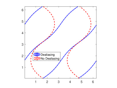
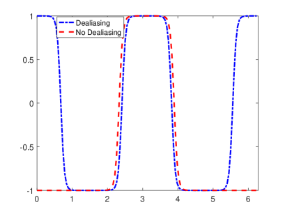
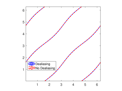
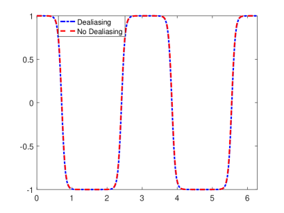
Figure 3.1: Example 3.1. Left: contour lines of $u$ with the value of $-0.1$; right: cut lines of the numerical solutions along $y=2\pi-x$ with $x\in[0,2\pi]$. Top: $N=128$; bottom: $N=256$.

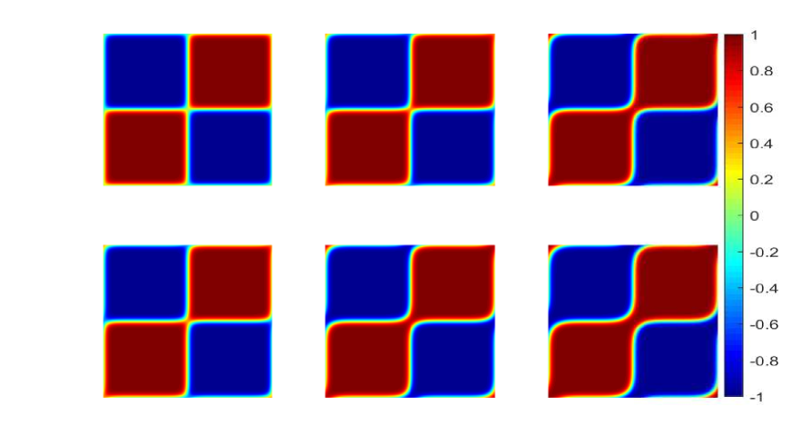
Figure 3.2: Example 3.1. Snapshots of the numerical solutions at $t=80$, $84$, and $88$ derived by SAV-M(3) with (Top) and without (Bottom) the de-aliasing.

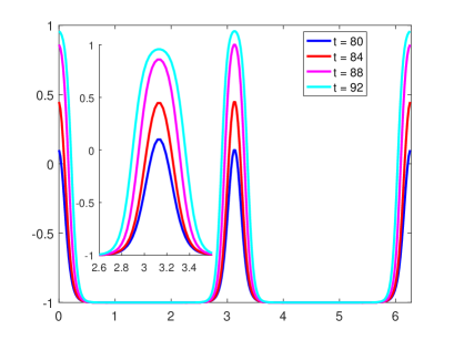
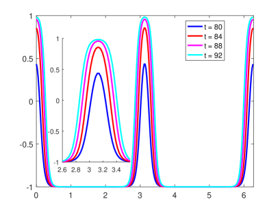
Figure 3.3: Example 3.1. Cut lines of the numerical solutions along $y=2\pi-x$, $x\in[0,2\pi]$, derived by SAV-M(3) with (Left) and without (Right) the de-aliasing.

Example 3.2.

This example is used to discuss the modified- and original-energy stabilities of SAV-M(1)$\sim$SAV-M(4) and G-SAV-M(1)$\sim$G-SAV-M(4) for the Allen-Cahn model (3.1). For this purpose, the domain $\Omega=(0,2\pi)\times(0,2\pi)$ is uniformly partitioned with $N=128$, the parameter $\epsilon=0.1$, and the initial value is chosen as $u(x,y,0)=0.1\times\mbox{\tt rand}(x,y)-0.05$, where $\mbox{\tt rand}(\cdot,\cdot)$ generates a random number between $0$ and $1$.

Figure 3.4 presents the discrete total modified-energy curves of SAV-M(1)$\sim$SAV-M(4) and G-SAV-M(1)$\sim$G-SAV-M(4) defined respectively in Theorem 2.3 and Remark 2.4. One can see that all those modified-energy curves are monotonically decreasing and consistent with the theoretical results. Figure 3.5 provides the discrete total original-energy curves of SAV-M(1)$\sim$SAV-M(4) and G-SAV-M(1)$\sim$G-SAV-M(4), and Figure 3.6 presents the numerical solution at $t=200$ derived by G-SAV-M(4) with $\tau=2$ and $1$. Those results show that the numerical solution shown in Figure 3.6 with $\tau=1$ is quite similar to that in [44], but when $\tau=2$, the solution is inaccurate or non-physical and the original energy is not monotonically decreasing as shown in Figure 3.5. It indicates that some time stepsize constraints are necessary to ensure the original-energy decay. Remark 3.1 will discuss the time stepsize constraints of SAV-M(1)$\sim$SAV-M(4) and G-SAV-M(1)$\sim$G-SAV-M(4) for the Allen-Cahn model (3.1) by using the stability regions of our SAV-GL schemes for the test equation.

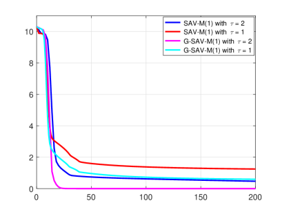
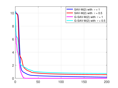
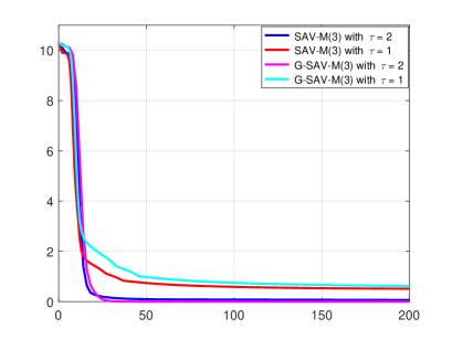
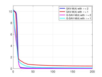
Figure 3.4: Example 3.2. The time evolution of the total modified-energies of SAV-M(1)$\sim$SAV-M(4) and G-SAV-M(1)$\sim$G-SAV-M(4) for the Allen-Cahn model (3.1).

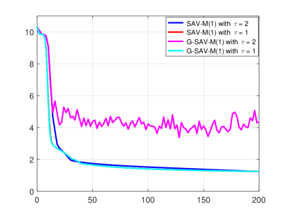
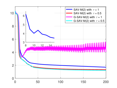
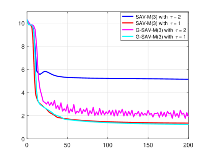
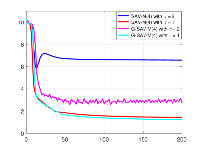
Figure 3.5: Same as Figure 3.4, except for the discrete total original-energies.

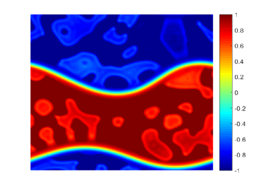
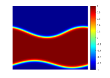
Figure 3.6: Example 3.2. Numerical solutions at $t=200$ computed by G-SAV-M(4) with $\tau=2$ (Left) and $1$ (Right), respectively.

Remark 3.1.

Applying the Fourier pseudo-spectral method to the Allen-Cahn model (3.1) yields the ODE system

$$\frac{d\hat{u}_{k,l}}{dt}=-\frac{4\pi^{2}\epsilon^{2}}{L^{2}}\left(k^{2}+l^{2}\right)\hat{u}_{k,l}+\hat{u}_{k,l}-\hat{w}_{k,l},~{}~{}~{}~{}(k,l)\in\widehat{\mathbb{S}}_{N},$$ (3.3)

where $\widehat{\mathbb{S}}_{N}=\left\{(k,l)\in\mathbb{Z}^{2}|-\frac{N}{2}+1\leq k,l\leq\frac{N}{2}\right\}$, $\{\hat{w}_{k,l}\}$ are the discrete Fourier coefficients of the cubic term $u^{3}$ and given by

$$\widehat{w}_{kl}=\frac{1}{N^{4}}\sum_{(m,n),(p,q)\in\widehat{\mathbb{S}}_{N}}\widehat{u}_{mn}\widehat{u}_{pq}\widehat{u}_{k-m-p,l-n-q}.$$ (3.4)

The system (3.3) may be viewed as the test equation (D.1) with $\xi=-\epsilon^{2}\left(k^{2}+l^{2}\right)$ and

$$\zeta=1-\frac{3}{N^{4}}\sum_{(m,n)\in\widehat{\mathbb{S}}_{N}}\hat{u}_{m,n}\hat{u}_{-m,-n}=1-\frac{3}{N^{4}}\sum_{(m,n)\in\widehat{\mathbb{S}}_{N}}|\hat{u}_{m,n}|^{2}=1-\frac{3}{N^{2}}\sum_{(i,j)\in\mathbb{S}_{N}}|u_{i,j}|^{2},$$

where $\mathbb{S}_{N}=\left\{(i,j)\in\mathbb{Z}^{2}|1\leq i,j\leq N\right\}$, $\hat{u}_{-m,-n}=\bar{\hat{u}}_{m,n}$ with $\bar{\hat{u}}_{m,n}$ being the complex conjugate of $\hat{u}_{-m,-n}$ and Parseval’s theorem have been used. For Example 3.2, Figure 3.7 plots the curve $\psi^{n}=\frac{3}{N^{2}}\sum\limits_{(i,j)\in\mathbb{S}_{N}}|u_{i,j}^{n}|^{2}$ derived by SAV-M(1)$\sim$SAV-M(4) and G-SAV-M(1)$\sim$G-SAV-M(4). It shows that $\psi^{n}\lesssim 2.7$ so that $\zeta\gtrsim-1.7$. Thus, one can take $\zeta\approx-1.7$ and then estimate the time stepsize according to D. Specifically, when the parameters $(\alpha_{0},\beta_{0},\beta_{2})=(0,0,1)$,

$$\tau<\min\left\{\frac{2}{(2\beta_{2}-1)\xi-(2\beta_{2}+1)\zeta}:\zeta<\frac{2\beta_{2}-1}{2\beta_{2}+1}\xi\right\}=\left\{\frac{2}{\max(\xi-3\zeta)}:\zeta<\frac{1}{3}\xi\right\},$$

which implies $\tau\lesssim 0.3922$ since $\max\{\xi-3\zeta:\zeta<\frac{1}{3}\xi\}=-3\zeta$; when $(\alpha_{0},\beta_{0},\beta_{2})=(-1/3,3/12,3/4)$,

$$\tau<\min\left\{\frac{1+\alpha_{0}}{(2\beta_{0}+\alpha_{0})\xi-\zeta}:\zeta<(2\beta_{0}+\alpha_{0})\xi\right\}=\left\{\frac{4}{3\max(\xi-2\zeta)}:\zeta<\frac{1}{2}\xi\right\},$$

which gives $\tau\lesssim 0.3922$ by using $\max\{\xi-2\zeta:\zeta<\frac{1}{2}\xi\}=-2\zeta$; when $(\alpha_{0},\beta_{0},\beta_{2})=(1/3,0,2/3)$,

$$\tau<\min\left\{\frac{1+\alpha_{0}}{(2\beta_{0}+\alpha_{0})\xi-\zeta}:\zeta<(2\beta_{0}+\alpha_{0})\xi\right\}=\left\{\frac{4}{\max(\xi-3\zeta)}:\zeta<\frac{1}{3}\xi\right\},$$

so that $\tau<-\frac{4}{3\zeta}\lesssim 0.7843$; and when $(\alpha_{0},\beta_{0},\beta_{2})=(1/3,-1/6,1/2)$,

$$\tau<-\frac{1+\alpha_{0}}{\zeta}\lesssim 0.7843.$$

Note that the above time stepsize constraints for SAV-M(1)$\sim$SAV-M(4) and G-SAV-M(1)$\sim$G-SAV-M(4) are sufficient and slightly more severer than them used in the numerical experiments on ensuring the original-energy decay of Example 3.2; and although the time discretization with $(\alpha_{0},\beta_{0},\beta_{2})=(1/3,-1/6,1/2)$ is not algebraically stable, the time stepsizes for SAV-M(4) and G-SAV-M(4) are comparable and both two schemes can provide good numerical results of (3.1). It is worth noting that for the Allen-Cahn model (3.1), one can use the maximum principle to give the estimation $\zeta\approx-2$, and then use D to get certain time stepsize conditions, which are also sufficient and have no big difference from the above estimations.

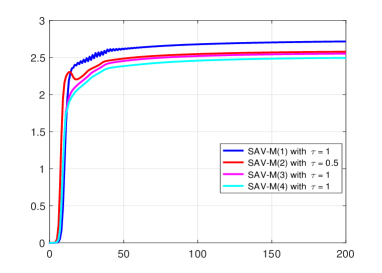
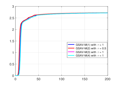
Figure 3.7: Example 3.2. $\psi^{n}$ derived by SAV-M(1)$\sim$SAV-M(4) (Left) and G-SAV-M(1)$\sim$G-SAV-M(4) (Right).

Remark 3.2.

For the SAV-GL scheme (LABEL:3.1.6), the term $\bar{\psi}^{n}=\frac{z^{n+\kappa}}{\sqrt{\mathcal{E}_{1}(\bar{u}^{n+\kappa})+C_{0}}}$ should be precisely considered in discussing the time stepsize constraints, theoretically. However, unfortunately, it is difficult to estimate exactly $\bar{\psi}^{n}$, even if it is equal to one at the continuous level. Figure 3.8 plots $\bar{\psi}^{n}$ derived by SAV-M(1)$\sim$SAV-M(4) with $\tau=1$ and $0.1$, from which one can observe $\bar{\psi}^{n}\lesssim 1$. This is the reason why we take $\bar{\psi}^{n}\approx 1$ for convenience and derive the time stepsize constraints for SAV-M(1)$\sim$SAV-M(4) in Remark 3.1.

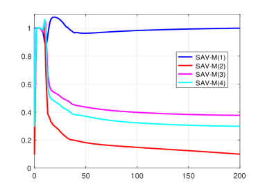
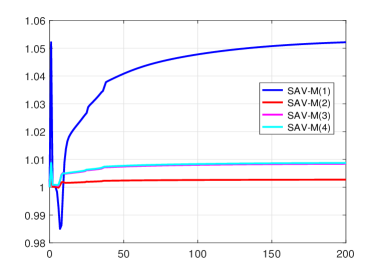
Figure 3.8: Example 3.2. $\bar{\psi}^{n}$ derived by SAV-M(1)$\sim$SAV-M(4) with $\tau=1$ (Left) and $0.1$ (Right), respectively.

3.2 Cahn-Hilliard model

The Cahn-Hilliard model

$$\frac{\partial u}{\partial t}=\Delta\left(-\epsilon^{2}\Delta u+u^{3}-u\right),~{}~{}~{}\mbox{\boldmath\small$x$}\in\Omega,~{}t>0,$$ (3.5)

is derived from the $H^{-1}$ gradient flow of the free energy (3.2), and describes the complicated phase separation and coarsening phenomena [6].

In order to apply SAV-M(1)$\sim$SAV-M(4) and G-SAV-M(1)$\sim$G-SAV-M(4) to the Cahn-Hilliard model (3.5), the operators $\mathcal{L}$, $\mathcal{G}$ and the energy $\mathcal{E}_{1}(u)$ are taken as

$$\mathcal{G}=\Delta,~{}~{}~{}\mathcal{L}=-\epsilon^{2}\Delta,~{}~{}~{}\mathcal{E}_{1}(u)=\int_{\Omega}\frac{1}{4}\left(u^{2}-1\right)^{2}dx.$$

Example 3.3.

This example is used to check the effectiveness of the de-aliasing by zero-padding for (3.5). We take $\epsilon=0.1$, and the initial data $u(x,y,0)=0.05\sin(x)\sin(y)$. The domain $\Omega=(0,2\pi)\times(0,2\pi)$ is partitioned with $N=128$ or $256$, and SAV-M(3) is used.

Figure 3.9 gives the contour lines and cut lines of the numerical solutions at $t=200$ derived by SAV-M(3) with or without de-aliasing. Visible difference between the numerical solutions with $N=128$ can be observed, but the difference is indistinguishable when $N=256$. For $N=256$, Figure 3.10 presents the snapshots of the numerical solutions at $t=7.5$, $8$, and $8.5$, while Figure 3.11 shows the cut lines of numerical solutions at $t=7.5,8,8.5$, and $9$. It is shown that there are some slight differences between those numerical solutions.

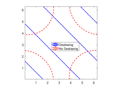
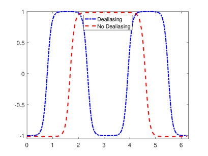
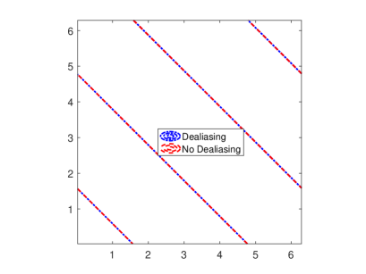
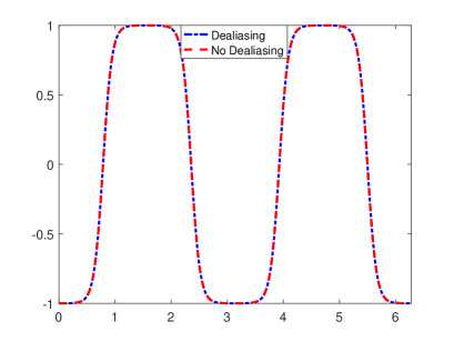
Figure 3.9: Example 3.3. Left: contour lines of $u$ with the value of $-0.1$; right: cut lines of the numerical solutions along $y=x$, $x\in[0,2\pi]$. Top: $N=128$; bottom: $N=256$.

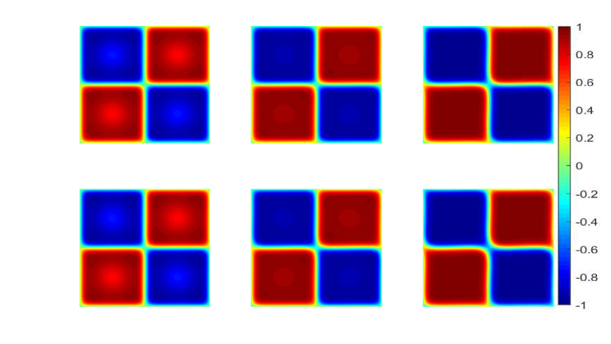
Figure 3.10: Example 3.3. Snapshots of the numerical solutions at $t=7.5,8$, and $8.5$ derived by SAV-M(3) with (Top) and without the de-aliasing (Bottom).

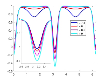
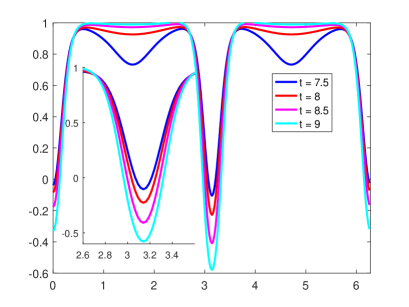
Figure 3.11: Example 3.3. Cut lines of the numerical solutions along $y=2\pi$, derived by SAV-M(3) with (Left) and without the de-aliasing (Right).

Example 3.4.

This example is used to validate the modified-energy stability and to check the original-energy stability of SAV-M(1)$\sim$SAV-M(4) and G-SAV-M(1)$\sim$G-SAV-M(4) for (3.5). The domain $\Omega=(0,2\pi)\times(0,2\pi)$ is uniformly partitioned with $N=128$, the parameter $\epsilon$ is taken as $0.1$, and the initial value is chosen as $u(x,y,0)=0.1\times\mbox{\tt rand}(x,y)-0.05$.

Figure 3.12 presents the discrete total modified-energy curves of SAV-M(1)$\sim$SAV-M(4) and G-SAV-M(1)$\sim$G-SAV-M(4). All those curves are monotonically decreasing, and consistent with the theoretical results. Figure 3.13 plots the discrete total original-energy curves of SAV-M(1)$\sim$SAV-M(4) and G-SAV-M(1)$\sim$G-SAV-M(4). The result shows that those schemes can ensure the original-energy decay only if a suitable time stepsize is taken. Figure 3.14 presents the numerical solutions at $t=200$ derived by G-SAV-M(2) with $\tau=0.02$ and $0.01$. It is shown that with a large time stepsize, the solution is inaccurate and the original-energy is not monotonically decreasing as shown in Figure 3.13. Remark 3.3 will provide a detailed discuss on the time stepsize constraints of SAV-M(1)$\sim$SAV-M(4) and G-SAV-M(1)$\sim$G-SAV-M(4) for the Cahn-Hilliard model (3.5).

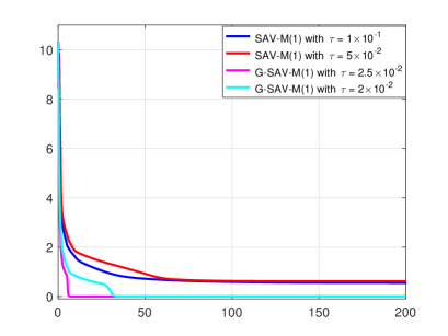
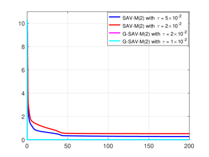
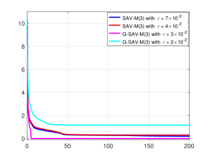
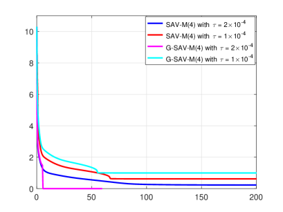
Figure 3.12: Example 3.4. The time evolution of the discrete total modified-energies of SAV-M(1)$\sim$SAV-M(4) and G-SAV-M(1)$\sim$G-SAV-M(4) for the Cahn-Hilliard model (3.5).

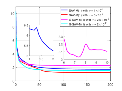
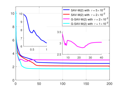
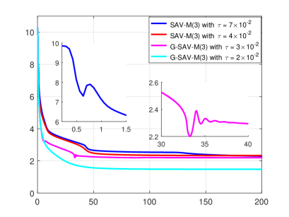
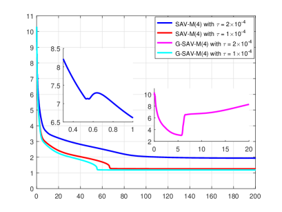
Figure 3.13: Same as Figure 3.12, except for the original-energy.

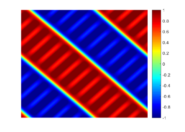
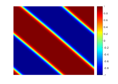
Figure 3.14: Example 3.4. Numerical solutions at $t=200$ derived by G-SAV-M(2) with $\tau=0.02$ (Left) and $0.01$ (Right), respectively.

Remark 3.3.

Applying the Fourier pseudo-spectral method to the Cahn-Hilliard model (3.5) yields the ODE system

$$\frac{d\hat{u}_{k,l}}{dt}=-\epsilon^{2}\left(k^{2}+l^{2}\right)^{2}\hat{u}_{k,l}-(k^{2}+l^{2})\left[\hat{w}_{k,l}-\hat{u}_{k,l}\right],~{}~{}~{}~{}(k,l)\in\widehat{\mathbb{S}}_{N},$$ (3.6)

where $\{\hat{w}_{k,l}\}$ are the discrete Fourier coefficients of the cubic term $u^{3}$ and given by (3.4). Similarly, (3.6) can also be viewed as the test equation (D.1) with

$$\xi=-\epsilon^{2}\left(k^{2}+l^{2}\right)^{2},~{}~{}~{}\zeta=-(k^{2}+l^{2})\left[\frac{3}{N^{2}}\sum\limits_{(i,j)\in\mathbb{S}_{N}}|u_{i,j}|^{2}-1\right],~{}~{}(k,l)\in\widehat{\mathbb{S}}_{N}.$$

For Example 3.4, the curves of $\psi^{n}=\frac{3}{N^{2}}\sum\limits_{(i,j)\in\mathbb{S}_{N}}|u_{i,j}|^{2}$ plotted in Figure 3.15 show that $\psi^{n}\lesssim 2.6$. Thus, one can take $\zeta\approx-1.6(k^{2}+l^{2}),(k,l)\in\widehat{\mathbb{S}}_{N}$ and then use D to estimate the time stepsizes for SAV-M(1)$\sim$SAV-M(4) and G-SAV-M(1)$\sim$G-SAV-M(4). Specifically, when the parameters $(\alpha_{0},\beta_{0},\beta_{2})=(0,0,1)$, the time stepsize satisfies

$$\tau<\left\{\frac{2}{\max(\xi-3\zeta)}:\zeta<\frac{1}{3}\xi\right\},$$

a simple calculation gives $\max\left\{\xi\!-\!3\zeta\right\}\!=\!\max\left\{-0.01\left(k^{2}\!+\!l^{2}\right)^{2}\!+\!4.8\left(k^{2}\!+\!l^{2}\right),(k,l)\in\widehat{\mathbb{S}}_{N}\right\}\!=\!575.99~{}(k\!=\!4,l\!=\!15)$ so that $\tau\lesssim 3.47\times 10^{-3}$; when $(\alpha_{0},\beta_{0},\beta_{2})=(-1/3,5/12,3/4)$,

$$\tau<\left\{\frac{4}{3\max(\xi-2\zeta)}:\zeta<\frac{1}{2}\xi\right\},$$

which is combined with the result $\max\left\{\xi\!-\!2\zeta\right\}\!=\!\max\!\left\{-0.01\left(k^{2}\!+\!l^{2}\right)^{2}\!+\!3.2\left(k^{2}\!+\!l^{2}\right),(k,l)\in\widehat{\mathbb{S}}_{N}\right\}\!=256~{}(k\!=\!4,l\!=\!12)$ to yield $\tau\lesssim 5.2\times 10^{-3}$; when $(\alpha_{0},\beta_{0},\beta_{2})=(1/3,0,2/3)$,

$$\tau<\left\{\frac{4}{\max(\xi-3\zeta)}:\zeta<\frac{1}{3}\xi\right\},$$

which gives $\tau\lesssim 7.0\times 10^{-3}$; and when $(\alpha_{0},\beta_{0},\beta_{2})=(1/3,-1/6,1/2)$,

$$\tau<-\frac{4}{3\min(\zeta)},$$

which gives $\tau\lesssim 1.02\times 10^{-4}$. Note that those time stepsize estimates for SAV-M(1)$\sim$SAV-M(4) and G-SAV-M(1)$\sim$G-SAV-M(4) are sufficient, and when $(\alpha_{0},\beta_{0},\beta_{2})=(1/3,-1/6,1/2)$, the GLTD is not algebraically stable and the time stepsize is constrained much severely for the Cahn-Hilliard model (3.5).

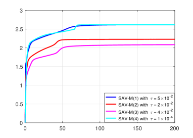
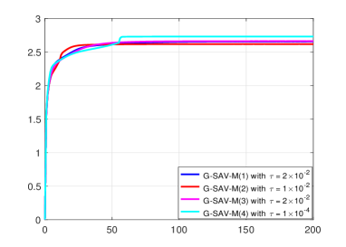
Figure 3.15: Example 3.4. $\psi^{n}$ derived by SAV-M(1)$\sim$SAV-M(4) (Left) and G-SAV-M(1)$\sim$G-SAV-M(4).

3.3 Phase field crystal model

The phase field crystal model

$$\frac{\partial u}{\partial t}=\Delta\mu,~{}~{}~{}\mu=u^{3}+(1-\epsilon)u+2\Delta u+\Delta^{2}u,~{}~{}~{}\mbox{\boldmath\small$x$}\in\Omega,~{}t>0,$$ (3.7)

can be derived from the $H^{-1}$ gradient flow of the free energy

$$\mathcal{E}(u)=\int_{\Omega}\left[\frac{1}{4}u^{4}+\frac{1-\epsilon}{2}u^{2}-|\nabla u|^{2}+\frac{1}{2}(\Delta u)^{2}\right]dx.$$

Such model may be used to describe many crystal phenomena such as edge dislocations [5], fcc ordering [50], epitaxial growth and zone refinement [15], and is a sixth-order nonlinear partial differential equation.

In order to apply SAV-M(1)$\sim$SAV-M(4) and G-SAV-M(1)$\sim$G-SAV-M(4) to (3.7) successfully, the operators $\mathcal{L}$, $\mathcal{G}$ and the energy $\mathcal{E}_{1}(u)$ are chosen as

$$\mathcal{L}=\Delta^{2},~{}~{}\mathcal{G}=\Delta,~{}~{}\mathcal{E}_{1}(u)=\int_{\Omega}\left[\frac{1}{4}u^{4}+\frac{1\!-\!\epsilon}{2}u^{2}-|\nabla u|^{2}\right]dx.$$

Example 3.5.

This example applies SAV-M(3) with or without the de-aliasing by zero-padding to the phase field crystal model (3.7). The parameter $\epsilon$ is taken as $0.25$, the domain $\Omega=(0,100)\times(0,100)$ is partitioned with $N=200$ or $400$, and the initial data is chosen as $u(x,y,0)=0.5\sin\left(\frac{\pi x}{50}\right)\sin\left(\frac{\pi y}{50}\right)$.

Figure 3.16 shows the contour lines and cut lines of the numerical solutions at $t=1000$ derived by SAV-M(3) with or without de-aliasing. Some visible differences between those numerical solutions with $N=200$ can be observed, but the differences are indistinguishable for $N=400$. Figure 3.17 gives the snapshots of the numerical solutions at $t=1000$ computed by SAV-M(3) with the de-aliasing. Figure 3.18 presents the cut lines of numerical solutions at $t=545$ and $670$. The results show that the numerical solutions by SAV-M(3) with or without the de-aliasing may have some differences at intermediate times.

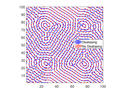
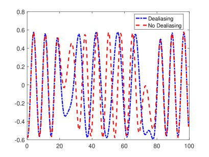
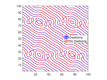
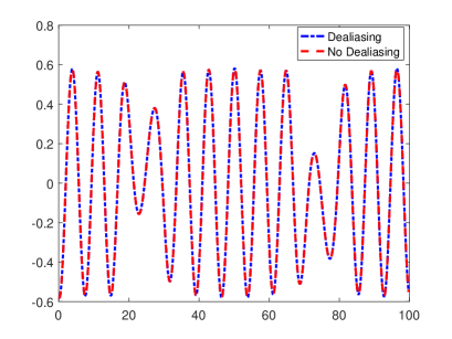
Figure 3.16: Example 3.5. Left: contour lines of $u$ with the value of $-0.1$; right: cut lines of the numerical solutions along $x=2\pi$. Top: $N=200$; bottom: $N=400$.

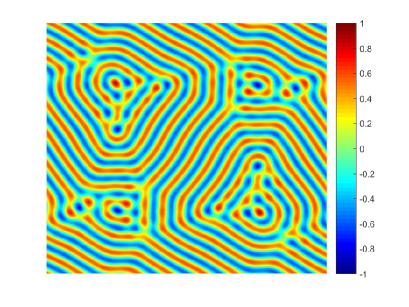
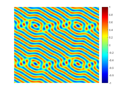
Figure 3.17: Example 3.5. Snapshots of the numerical solutions at $t=1000$ derived by SAV-M(3) with the de-aliasing. Left: $N=200$; right: $N=400$.

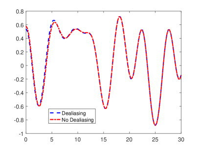
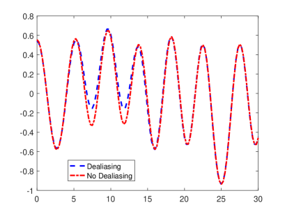
Figure 3.18: Example 3.5. Cut lines of the numerical solutions along $y=x$, $x\in[0,30]$, at $t=545$ (Left) and $t=670$ (Right).

Example 3.6.

It simulates the polycrystal growth in a supercool liquid and investigates the modified- and original-energy stabilities of SAV-M(1)$\sim$SAV-M(4) and G-SAV-M(1)$\sim$G-SAV-M(4). For this purpose, the domain $\Omega=(0,400)\times(0,400)$ is partitioned with $N=400$, the parameter $\epsilon=0.25$, and the initial value is taken as (see e.g. [34])

$$u(x,y,0)=\begin{cases}\phi_{0}\!+\!B\!\left[\cos\!\left(\frac{\sqrt{6}\vartheta}{6}(y\!-\!x)\right)\cos\!\left(\!\frac{\sqrt{2}\vartheta}{2}(x\!+\!y)\right)\!\!-\!\frac{1}{2}\cos\!\left(\!\frac{\sqrt{6}\vartheta}{3}(y\!-\!x)\right)\!\right]\!,~{}~{}(x,y)\!\in\!\Omega_{1},\\[3.0pt] \phi_{0}\!+\!B\!\left[\cos\!\left(\frac{\sqrt{6}\vartheta}{6}(x\!+\!y)\right)\cos\!\left(\!\frac{\sqrt{2}\vartheta}{2}(y\!-\!x)\right)\!\!-\!\frac{1}{2}\cos\!\left(\!\frac{\sqrt{6}\vartheta}{3}(x\!+\!y)\right)\!\right]\!,~{}~{}(x,y)\!\in\!\Omega_{2},\\ \phi_{0}\!+\!B\!\left[\cos\!\left(\frac{\vartheta}{\sqrt{3}}x\right)\cos\!\left(\!\vartheta y\right)\!\!-\!\frac{1}{2}\cos\!\left(\!\frac{2\vartheta}{\sqrt{3}}x\right)\!\right]\!,~{}~{}(x,y)\!\in\!\Omega_{3},\\[3.0pt] \phi_{0},~{}~{}(x,y)\!\in\!\Omega\backslash(\Omega_{1}\cup\Omega_{2}\cup\Omega_{3}),\end{cases}$$

where $\phi_{0}=0.285$, $B=0.446$, $\vartheta=0.66$, $\Omega_{1}=[130,170]\times[130,170]$, $\Omega_{2}=[230,270]\times[130,170]$, and $\Omega_{3}=[180,220]\times[230,270]$.

Figure 3.19 presents the discrete total modified-energy curves of SAV-M(1)$\sim$SAV-M(4) and G-SAV-M(1)$\sim$G-SAV-M(4). They are monotonically decreasing, and consistent with the theoretical results. Figure 3.20 shows the discrete total original-energy curves of SAV-M(1)$\sim$SAV-M(4) and G-SAV-M(1)$\sim$G-SAV-M(4) for (3.7). It is shown that those schemes can preserve the original-energy decay if a suitable time stepsize is chosen. Figure 3.21 gives the numerical solution at $t=2400$ derived by G-SAV-M(4) with $\tau=15$ and $12$. One can find the numerical solution derived by G-SAV-M(4) with $\tau=12$ is similar to that in [34, 44], but when $\tau=15$, an the solution is inaccurate and the original-energy is not monotonically decreasing. Remark 3.4 will discuss the time stepsize constraints of SAV-M(1)$\sim$SAV-M(4) and G-SAV-M(1)$\sim$G-SAV-M(4) for the phase field crystal model (3.7).

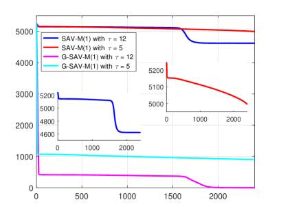
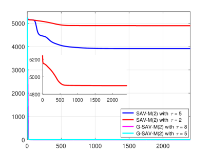
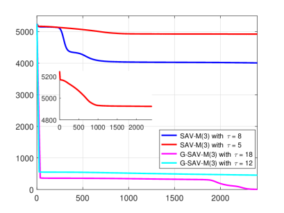
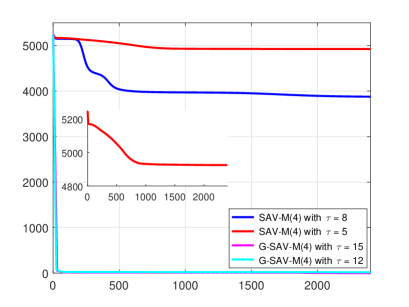
Figure 3.19: Example 3.6. The discrete total modified-energy curves of SAV-M(1)$\sim$SAV-M(4) and G-SAV-M(1)$\sim$G-SAV-M(4) for the phase field crystal model (3.7).

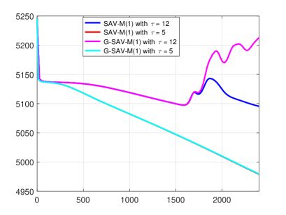
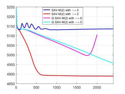
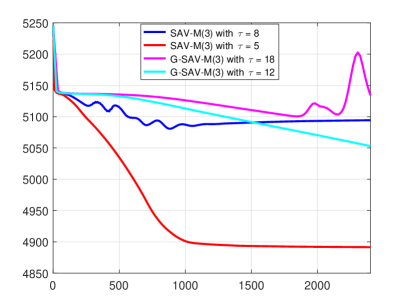
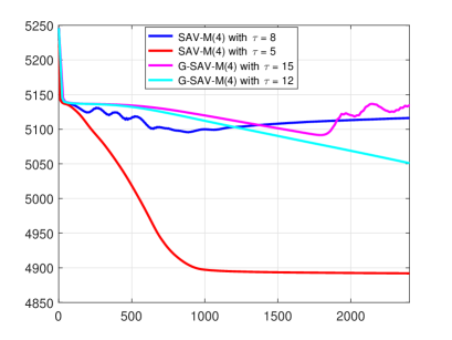
Figure 3.20: Same as Figure 3.19, except for the original-energy.

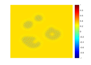
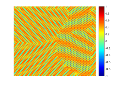
Figure 3.21: Example 3.6. Numerical solutions at $t=2400$ derived by G-SAV-M(4) with $\tau=15$ (Left) and $12$ (Right), respectively.

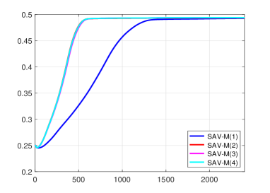
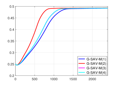
Figure 3.22: Example 3.6. $\psi^{n}$ (y-axis) derived by SAV-M(1)$\sim$SAV-M(4) (Left) and G-SAV-M(1)$\sim$G-SAV-M(4) with $\tau=1$.

Remark 3.4.

This remark discusses the time stepsize constraints of SAV-M(1)$\sim$SAV-M(4) and G-SAV-M(1)$\sim$G-SAV-M(4) for the phase field crystal model (3.7).

Applying the Fourier pseudo-spectral method to (3.7) yields the ODE system

$$\frac{d\hat{u}_{k,l}}{dt}=-\frac{\pi^{3}\left(k^{2}\!+\!l^{2}\right)^{3}}{200^{3}}\hat{u}_{k,l}-\frac{\pi(k^{2}\!+\!l^{2})}{200}\left[\hat{w}_{k,l}+\frac{3}{8}\hat{u}_{k,l}-\frac{\pi(k^{2}\!+\!l^{2})}{100}\hat{u}_{k,l}\right],$$ (3.8)

where $\{\hat{w}_{k,l},(k,l)\in\widehat{\mathbb{S}}_{N}\}$ are the discrete Fourier coefficients of the cubic term $u^{3}$ and given by (3.4). Similarly, (3.8) can be viewed as the test equation (D.1) with

$$\xi=-\frac{\pi^{3}\left(k^{2}+l^{2}\right)^{3}}{200^{3}},~{}~{}~{}\zeta=-\frac{\pi(k^{2}\!+\!l^{2})}{200}\!\left[\frac{3}{N^{2}}\!\sum\limits_{(i,j)\in\mathbb{S}_{N}}\!|u_{i,j}|^{2}\!+\!\frac{3}{8}\!-\!\frac{\pi(k^{2}\!+\!l^{2})}{100}\right]\!,~{}~{}~{}(k,l)\in\widehat{\mathbb{S}}_{N}.$$

For Example 3.6, Figure 3.22 gives the curves of $\psi^{n}=\frac{3}{N^{2}}\sum\limits_{(i,j)\in\mathbb{S}_{N}}|u_{i,j}|^{2}$ derived by SAV-M(1)$\sim$SAV-M(4) and G-SAV-M(1)$\sim$G-SAV-M(4) with $\tau=1$. It is shown that $\psi^{n}\leq 0.5$ so that $\zeta\geq-\frac{\pi(k^{2}+l^{2})}{200}\!\left[\frac{7}{8}\!-\!\frac{\pi(k^{2}+l^{2})}{100}\right]$. In the following, one may take $\zeta\approx-\frac{\pi(k^{2}+l^{2})}{200}\!\left[\frac{7}{8}\!-\!\frac{\pi(k^{2}+l^{2})}{100}\right]$ and use D to discuss the time stepsize constraints for SAV-M(1)$\sim$SAV-M(4) and G-SAV-M(1)$\sim$G-SAV-M(4). Specifically, when $(\alpha_{0},\beta_{0},\beta_{2})=(0,0,1)$, it requires

$$\tau<\left\{\frac{2}{\max(\xi-3\zeta)}:\zeta<\frac{1}{3}\xi\right\},$$

and a simple calculation shows that when $k=3$ and $l=2$, $\max\left\{\xi-3\zeta\right\}=0.2788$, which gives $\tau\lesssim 7.21$; when $(\alpha_{0},\beta_{0},\beta_{2})=(-1/3,5/12,3/4)$,

$$\tau<\left\{\frac{4}{3\max(\xi-2\zeta)}:\zeta<\frac{1}{2}\xi\right\},$$

which is combined with $\max\left\{\xi-2\zeta\right\}=0.2964$ for $k=2$ and $l=3$ to get $\tau\lesssim 7.32$; when $(\alpha_{0},\beta_{0},\beta_{2})=(1/3,0,2/3)$,

$$\tau<\left\{\frac{4}{\max(\xi-3\zeta)}:\zeta<\frac{1}{3}\xi\right\},$$

so that $\tau\lesssim 14.42$; and when $(\alpha_{0},\beta_{0},\beta_{2})=(1/3,-1/6,1/2)$,

$$\tau<-\frac{4}{3\min(\zeta)},$$

which yields $\tau\lesssim 13.99$ since $\min(\zeta)=0.1524$ for $k=3$ and $l=2$. Note that those time stepsize estimates for SAV-M(1)$\sim$SAV-M(4) and G-SAV-M(1)$\sim$G-SAV-M(4) are sufficient. Compared to the numerical results shown in Figure 3.20, one needs to take slightly smaller time stepsizes to ensure the original-energy decay when SAV-M(1)$\sim$SAV-M(4) are applied to (3.7), but the above time stepsize estimates are almost consistent with those in numerical experiments for G-SAV-M(1)$\sim$G-SAV-M(4).

4 Conclusion

This paper continued to study linear and unconditionally modified-energy stable numerical schemes (abbreviated as SAV-GL) for the gradient flows. Those schemes were built on the SAV technique and the general linear time discretizations (GLTD) as well as the extrapolation for the nonlinear term, and two linear systems with the same constant coefficient were solved at each time step. Different from [44], the GLTDs with three parameters discussed here were not necessarily algebraically stable. Some algebraic identities were first derived by using the method of undetermined coefficients and then used to establish the modified-energy inequalities for the unconditional modified-energy stability of the semi-discrete-in-time SAV-GL schemes. It was worth emphasizing that those algebraic identities or energy inequalities are not necessarily unique for some choices of three parameters in the GLTDs. In order to demonstrate numerically the energy stability of our SAV-GL schemes, the Fourier pseudo-spectral spatial discretization was employed for the gradient flow models with periodic boundary conditions. The effect of the aliasing error and the de-aliasing by zero-padding provided in C on the numerical results were investigated.

Numerical experiments were conducted on the Allen-Cahn, the Cahn-Hilliard, and the phase field crystal models, and well demonstrated the unconditional modified-energy stability of SAV-M(1)$\sim$ SAV-M(4) in comparison to another SAV-GL schemes (abbreviated as G-SAV-M(1)$\sim$ G-SAV-M(4)) built on the generalized SAV and the effectiveness of the de-aliasing by zero-padding. Numerical results also showed that a suitable time stepsize were required for the SAV-GL schemes to ensure the original-energy decay. With the help of discussing the stability regions for the semi-implicit SAV-GL schemes applied to the test equation in D, the time stepsizes for SAV-M(1)$\sim$ SAV-M(4) were estimated for the Allen-Cahn, the Cahn-Hilliard, and the phase field crystal models. Our computations showed that those time stepsize constraints could ensure the original-energy decay essentially.

Appendix A Proof of Lemma 2.1

This appendix proves Lemma 2.1 by discussing the $A$-stability conditions of the fully implicit time discretizations based on (2.3)-(2.4).

Applying (2.3)-(2.4) to the test equation

$$\frac{du}{dt}=u^{\prime}(t)=\xi u(t),~{}~{}t\in(0,T],~{}~{}u(0)=u_{0},$$

yields

$$\frac{1}{1\!-\!\alpha_{0}}u_{n+1}-\frac{1\!+\!\alpha_{0}}{1\!-\!\alpha_{0}}u_{n}+\frac{\alpha_{0}}{1\!-\!\alpha_{0}}u_{n-1}=\bar{\xi}\left[\frac{\beta_{2}}{1\!-\!\alpha_{0}}u_{n+1}+\frac{\beta_{1}}{1\!-\!\alpha_{0}}u_{n}+\frac{\beta_{0}}{1\!-\!\alpha_{0}}u_{n-1}\right],$$ (A.1)

where $\bar{\xi}=\xi\tau$, $\xi$ is a complex number, and the symbol $u_{n}$ have been temporarily used to replace the previous approximate solution $u^{n}$ for convenience. Substituting $u_{j}=x^{j}$ into (A.1) and dividing by $x^{n-1}$ give the characteristic equation

$$\rho(x)-\bar{\xi}\sigma(x)=0,$$ (A.2)

with

$$\rho(x)=\frac{1}{1\!-\!\alpha_{0}}x^{2}-\frac{1\!+\!\alpha_{0}}{1\!-\!\alpha_{0}}x+\frac{\alpha_{0}}{1\!-\!\alpha_{0}},~{}~{}~{}\sigma(x)=\frac{\beta_{2}}{1\!-\!\alpha_{0}}x^{2}+\frac{\beta_{1}}{1\!-\!\alpha_{0}}x+\frac{\beta_{0}}{1\!-\!\alpha_{0}}.$$

According to [24, Def. 1.1], the scheme (A.1) is $A$-stable iff for any $\bar{\xi}\in\mathbb{C}^{-}$, all solutions of (A.2) are smaller or equal to one in modulus, and the multiple solutions are strictly smaller than one. It is known that all roots of the polynomial $c_{2}x^{2}+c_{1}x+c_{0}$ are smaller or equal to one in modulus iff $|c_{0}|\leq|c_{2}|$ and $|c_{1}|\leq|c_{0}+c_{2}|$, see e.g. [7]. Thus, when

$$\left|\alpha_{0}-\beta_{0}\bar{\xi}\right|\leq\left|1-\beta_{2}\bar{\xi}\right|,~{}~{}~{}\left|1+\alpha_{0}-\beta_{1}\bar{\xi}\right|\leq\left|1+\alpha_{0}-\left(\beta_{0}\!+\!\beta_{2}\right)\bar{\xi}\right|,$$ (A.3)

for any $\bar{\xi}\in\mathbb{C}^{-}$, all roots of the characteristic polynomial

$$\mathbb{P}(x):=\rho(x)-\bar{\xi}\sigma(x)=\left(\frac{1}{1\!-\!\alpha_{0}}-\frac{\beta_{2}}{1\!-\!\alpha_{0}}\bar{\xi}\right)x^{2}-\left(\frac{1\!+\!\alpha_{0}}{1\!-\!\alpha_{0}}-\frac{\beta_{1}}{1\!-\!\alpha_{0}}\bar{\xi}\right)x+\frac{\alpha_{0}}{1\!-\!\alpha_{0}}-\frac{\beta_{0}}{1\!-\!\alpha_{0}}\bar{\xi},$$

are smaller or equal to one in modulus so that the scheme (A.1) is $A$-stable. Let $\bar{\xi}=a+\imath b$ with $\imath=\sqrt{-1}$, $a\leq 0$ and $b\in\mathbb{R}$. The first inequality in (A.3) is equivalent to

$$2a(\alpha_{0}\beta_{0}\!-\!\beta_{2})\!+\!\left(\beta_{2}^{2}\!-\!\beta_{0}^{2}\right)\left(a^{2}\!+\!b^{2}\right)\!+\!1\!-\!\alpha_{0}^{2}\geq 0,~{}~{}~{}\forall~{}a\leq 0,~{}b\in\mathbb{R}.$$

A direct check shows that the parameters $\alpha_{0},\beta_{0}$ and $\beta_{2}$ should satisfy

$$-1\leq\alpha_{0}<1,~{}~{}~{}\alpha_{0}\beta_{0}\leq\beta_{2},~{}~{}~{}|\beta_{0}|\leq|\beta_{2}|,$$

which further gives

$$-1\leq\alpha_{0}<1,~{}~{}~{}\beta_{2}>0,~{}~{}~{}|\beta_{0}|\leq\beta_{2}.$$ (A.4)

On the other hand, the second inequality in (A.3) is equivalent to

$$\left(2\beta_{0}\!+\!2\beta_{2}\!+\!\alpha_{0}\!-\!1\right)\left(1\!-\!\alpha_{0}\right)(a^{2}\!+\!b^{2})\!+\!2(1\!+\!\alpha_{0})\left(1\!-\!\alpha_{0}\!-\!2\beta_{0}\!-\!2\beta_{2}\right)a\!\geq\!0,~{}~{}~{}\forall~{}a\leq 0,~{}b\in\mathbb{R},$$

which yields

$$\left(2\beta_{0}\!+\!2\beta_{2}\!+\!\alpha_{0}\!-\!1\right)\left(1\!-\!\alpha_{0}\right)\geq 0,~{}~{}~{}(1\!+\!\alpha_{0})\left(1\!-\!\alpha_{0}\!-\!2\beta_{0}\!-\!2\beta_{2}\right)\leq 0.$$ (A.5)

Combining (A.4) with (A.5) yields that the scheme (A.1) is $A$-stable when the parameters $\alpha_{0},\beta_{0}$ and $\beta_{2}$ satisfy

$$-1\leq\alpha_{0}<1,~{}~{}~{}\beta_{2}>0,~{}~{}~{}|\beta_{0}|\leq\beta_{2},~{}~{}~{}1-\alpha_{0}-2\beta_{0}-2\beta_{2}\leq 0.$$ (A.6)

Some special cases are discussed as follows.

$\bullet$ When $\alpha_{0}=\beta_{0}=0$, (A.1) reduces to a one-step scheme with parameter $\beta_{2}$, i.e,

$$u_{n+1}-u_{n}=\beta_{2}\bar{\xi}u_{n+1}+(1\!-\!\beta_{2})\bar{\xi}u_{n},$$ (A.7)

which is second-order accurate only for $\beta_{2}=\frac{1}{2}$. A direct check shows that the condition (A.6) becomes $\beta_{2}\geq\frac{1}{2}$, under which (A.7) is $A$-stable.

$\bullet$ When $\beta_{2}=\frac{1}{2}(1+\alpha_{0})+\beta_{0}$, and $\alpha_{0}$ and $\beta_{0}$ are not zero simultaneously, (A.1) reduces to a class of two-step and second-order schemes, i.e.,

$$\frac{1}{1\!-\!\alpha_{0}}u_{n+1}\!-\!\frac{1\!+\!\alpha_{0}}{1\!-\!\alpha_{0}}u_{n}\!+\!\frac{\alpha_{0}}{1\!-\!\alpha_{0}}u_{n-1}\!=\!\bar{\xi}\left[\frac{1\!+\!\alpha_{0}\!+\!2\beta_{0}}{2(1\!-\!\alpha_{0})}u_{n+1}\!+\!\frac{1\!-\!3\alpha_{0}\!-\!4\beta_{0}}{2(1\!-\!\alpha_{0})}u_{n}\!+\!\frac{\beta_{0}}{1\!-\!\alpha_{0}}u_{n-1}\!\right]\!.$$ (A.8)

It can be seen that (A.6) is simplified as $-1\leq\alpha_{0}<1$ and $2\beta_{0}+\alpha_{0}\geq 0$, under which the scheme (A.8) is $A-$stable. Moreover, if taking $\alpha_{0}=\frac{\lambda-1}{\lambda+1},$ $\beta_{0}=\frac{1-\lambda+\delta}{2(1+\lambda)},\beta_{2}=\frac{1+\lambda+\delta}{2(1+\lambda)}$, then (A.8) is rewritten into

$$\frac{1+\lambda}{2}u_{n+1}-\lambda u_{n}+\frac{\lambda-1}{2}u_{n-1}=\bar{\xi}\left[\frac{1+\lambda+\delta}{4}u_{n+1}+\frac{1-\delta}{2}u_{n}+\frac{1-\lambda+\delta}{4}u_{n-1}\right],$$ (A.9)

so that it is $A-$stable for any $\lambda\geq 0$, $\delta\geq 0$.

$\bullet$ When $\beta_{2}\neq\frac{1}{2}(1+\alpha_{0})+\beta_{0}$, and $\alpha_{0}$ and $\beta_{0}$ are not zero simultaneously, (A.1) is two-step but only first-order accurate. In this case, the condition (A.6) can not be simplified.

When the scheme (A.1) is $A$-stable, it may not be algebraically stable. For example, the scheme (A.9) with $\lambda\geq 0$ and $\delta>0$ is shown to be algebraically stable with the positive definite matrix

$$\mbox{\boldmath\small$G$}=\frac{1}{4}\!\left(\!\begin{array}[]{*{4}{c}}(1+\lambda)^{2}+\delta&1-\delta-\lambda^{2}\\ 1-\delta-\lambda^{2}&(\lambda-1)^{2}+\delta\end{array}\!\right),$$

see e.g. [13], but it is not algebraically stable when $\lambda\geq 0$ and $\delta=0$. In fact, if (A.9) with $\lambda\geq 0$ and $\delta=0$ is algebraically stable, then Theorem 3.2 in [13] shows that corresponding matrix $\bar{\mbox{\boldmath\small$G$}}$ should satisfy

$$(1,1)\bar{\mbox{\boldmath\small$G$}}=\frac{1}{2}\left(1\!+\!\lambda,1\!-\!\lambda\right),~{}~{}~{}(1,0)\bar{\mbox{\boldmath\small$G$}}=\frac{1}{4}\left((1\!+\!\lambda)^{2},1\!-\!\lambda^{2}\right),$$

which uniquely gives

$$\bar{\mbox{\boldmath\small$G$}}=\frac{1}{4}\!\left(\!\begin{array}[]{*{4}{c}}(1+\lambda)^{2}&1-\lambda^{2}\\ 1-\lambda^{2}&(\lambda-1)^{2}\end{array}\!\right).$$

Obviously, $\bar{\mbox{\boldmath\small$G$}}$ is not positive definite so that (A.9) with $\lambda\geq 0$ and $\delta=0$ is not algebraically stable. Thus, when $\beta_{2}=\frac{1}{2}(1+\alpha_{0})+\beta_{0}$, and $\alpha_{0}$ and $\beta_{0}$ are not zero simultaneously, (A.1) is algebraically stable for any $-1\leq\alpha_{0}<1$ and $2\beta_{0}+\alpha_{0}>0$, but is not algebraically stable for $-1\leq\alpha_{0}<1$ and $2\beta_{0}+\alpha_{0}=0$. ∎

Appendix B Proof of Lemma 2.2

This appendix proves Lemma 2.2, which plays an important role for the modified-energy stability of the SAV-GL scheme (LABEL:3.1.6), whose time discretization is not necessarily algebraically stable.

The establishment of the identities (2.8)-(2.2) in Lemma 2.2 is motivated by the identities in [41, 54], and may be completed by using the method of undetermined coefficients. Suppose the parameters $\alpha_{0},\beta_{0}$, and $\beta_{2}$ in (2.3)-(2.5) satisfy the condition (A.6). In order to derive the modified-energy stability of our SAV-GL scheme (LABEL:3.1.6), we expect the following identity

$$\big{(}\frac{1}{1\!-\!\alpha_{0}}\chi^{n+1}- \frac{1\!+\!\alpha_{0}}{1\!-\!\alpha_{0}}\chi^{n}+\frac{\alpha_{0}}{1\!-\!\alpha_{0}}\chi^{n-1}\big{)}\big{(}\frac{\beta_{2}}{1\!-\!\alpha_{0}}\chi^{n+1}+\frac{\beta_{1}}{1\!-\!\alpha_{0}}\chi^{n}+\frac{\beta_{0}}{1\!-\!\alpha_{0}}\chi^{n-1}\big{)}$$

$$=\; a\left[\left(\chi^{n+1}\right)^{2}-\left(\chi^{n}\right)^{2}\right]+b\left[\left(\chi^{n}\right)^{2}-\left(\chi^{n-1}\right)^{2}\right]+d\left[\chi^{n+1}\chi^{n}-\chi^{n}\chi^{n-1}\right]$$

$$+\left(c_{1}\chi^{n+1}+c_{2}\chi^{n}+c_{3}\chi^{n-1}\right)^{2},$$ (B.1)

where $a,b,d$ and $c_{i},i=1,2,3$ are six undetermined real coefficients. Expanding the term at the left hand side of (B) and then comparing each coefficient with that at the right hand side yield

$$\begin{aligned} &a+c_{1}^{2}=\frac{\beta_{2}}{(1-\alpha_{0})^{2}},~{}~{}~{}b-a+c_{2}^{2}=-\frac{(1+\alpha_{0})\beta_{1}}{(1-\alpha_{0})^{2}},\\[3.0pt] &c_{3}^{2}-b=\frac{\alpha_{0}\beta_{0}}{(1-\alpha_{0})^{2}},~{}~{}~{}2c_{1}c_{2}+d=\!\frac{\beta_{1}}{(1-\alpha_{0})^{2}}-\frac{(1+\alpha_{0})\beta_{2}}{(1-\alpha_{0})^{2}},\\[3.0pt] &2c_{2}c_{3}-d=\frac{\alpha_{0}\beta_{1}}{(1-\alpha_{0})^{2}}-\frac{(1+\alpha_{0})\beta_{0}}{(1-\alpha_{0})^{2}},~{}~{}~{}2c_{1}c_{3}=\frac{\beta_{0}}{(1-\alpha_{0})^{2}}+\frac{\alpha_{0}\beta_{2}}{(1-\alpha_{0})^{2}}.\end{aligned}$$ (B.2)

Adding all six equations gives $(c_{1}+c_{2}+c_{3})^{2}=0$, which implies

$$c_{1}+c_{2}+c_{3}=0.$$ (B.3)

The fourth and fifth equations in (B.2) may gives

$$2c_{2}(c_{1}+c_{3})\!=\!\frac{(1+\alpha_{0})(\beta_{1}-\beta_{0}-\beta_{2})}{(1-\alpha_{0})^{2}},$$

which is combined with (B.3) to give $c_{2}\!=\!\pm\frac{\sqrt{2(1+\alpha_{0})(\beta_{0}+\beta_{2}-\beta_{1})}}{2(1-\alpha_{0})}$. Note that $(1+\alpha_{0})(\beta_{0}+\beta_{2}-\beta_{1})=(1+\alpha_{0})(2\beta_{0}+2\beta_{2}+\alpha_{0}-1)\geq 0$ when the condition (A.6) holds. If substituting $c_{2}$ into (B.3) and combining it with the sixth equation in (B.2), then it is obvious that $c_{1}$ and $c_{3}$ are two solutions of $x^{2}+c_{2}x+\frac{\beta_{0}+\alpha_{0}\beta_{2}}{2(1-\alpha_{0})^{2}}=0$, so that

$$c_{1}=-\frac{c_{2}}{2}+\sqrt{\frac{c_{2}^{2}}{4}-\frac{\beta_{0}\!+\!\alpha_{0}\beta_{2}}{2(1\!-\!\alpha_{0})^{2}}}~{}~{}~{}~{}c_{3}=-\frac{c_{2}}{2}-\sqrt{\frac{c_{2}^{2}}{4}-\frac{\beta_{0}\!+\!\alpha_{0}\beta_{2}}{2(1\!-\!\alpha_{0})^{2}}},$$

or

$$c_{1}=-\frac{c_{2}}{2}-\sqrt{\frac{c_{2}^{2}}{4}-\frac{\beta_{0}\!+\!\alpha_{0}\beta_{2}}{2(1\!-\!\alpha_{0})^{2}}},~{}~{}~{}~{}c_{3}=-\frac{c_{2}}{2}+\sqrt{\frac{c_{2}^{2}}{4}-\frac{\beta_{0}\!+\!\alpha_{0}\beta_{2}}{2(1\!-\!\alpha_{0})^{2}}}.$$

We expect that the term $\frac{c_{2}^{2}}{4}-\frac{\beta_{0}+\alpha_{0}\beta_{2}}{2(1-\alpha)^{2}}$ is non-negative so that both $c_{1}$ and $c_{3}$ are real, and will discuss that in three cases below. If $\frac{c_{2}^{2}}{4}-\frac{\beta_{0}+\alpha_{0}\beta_{2}}{2(1-\alpha)^{2}}$ is non-negative, then inserting $c_{1}$ and $c_{3}$ into the first, third and fifth equations in (B.2) yields

$$a=\frac{2\beta_{2}\!+\!\beta_{0}\!+\!\alpha_{0}\beta_{2}}{2(1\!-\!\alpha_{0})^{2}}-\frac{c_{2}^{2}}{2}+c_{2}\sqrt{\frac{c_{2}^{2}}{4}-\frac{\beta_{0}\!+\!\alpha_{0}\beta_{2}}{2(1\!-\!\alpha_{0})^{2}}},$$

$$b=-\frac{\alpha_{0}\beta_{0}\!+\!\beta_{0}\!+\!\alpha_{0}\beta_{2}}{2(1\!-\!\alpha_{0})^{2}}+\frac{c_{2}^{2}}{2}+c_{2}\sqrt{\frac{c_{2}^{2}}{4}-\frac{\beta_{0}\!+\!\alpha_{0}\beta_{2}}{2(1\!-\!\alpha_{0})^{2}}},$$

$$d=-\frac{\alpha_{0}\beta_{1}\!-\!(1\!+\!\alpha_{0})\beta_{0}}{(1\!-\!\alpha_{0})^{2}}-c_{2}^{2}-2c_{2}\sqrt{\frac{c_{2}^{2}}{4}-\frac{\beta_{0}\!+\!\alpha_{0}\beta_{2}}{2(1\!-\!\alpha_{0})^{2}}},$$

or

$$a=\frac{2\beta_{2}\!+\!\beta_{0}\!+\!\alpha_{0}\beta_{2}}{2(1\!-\!\alpha_{0})^{2}}-\frac{c_{2}^{2}}{2}-c_{2}\sqrt{\frac{c_{2}^{2}}{4}-\frac{\beta_{0}\!+\!\alpha_{0}\beta_{2}}{2(1\!-\!\alpha_{0})^{2}}},$$

$$b=-\frac{\alpha_{0}\beta_{0}\!+\!\beta_{0}\!+\!\alpha_{0}\beta_{2}}{2(1\!-\!\alpha_{0})^{2}}+\frac{c_{2}^{2}}{2}-c_{2}\sqrt{\frac{c_{2}^{2}}{4}-\frac{\beta_{0}\!+\!\alpha_{0}\beta_{2}}{2(1\!-\!\alpha_{0})^{2}}},$$

$$d=-\frac{\alpha_{0}\beta_{1}\!-\!(1\!+\!\alpha_{0})\beta_{0}}{(1\!-\!\alpha_{0})^{2}}-c_{2}^{2}+2c_{2}\sqrt{\frac{c_{2}^{2}}{4}-\frac{\beta_{0}\!+\!\alpha_{0}\beta_{2}}{2(1\!-\!\alpha_{0})^{2}}}.$$

Those undetermined coefficients can give the final identity (B), which may be not unique.

Let us discuss when $\frac{c_{2}^{2}}{4}-\frac{\beta_{0}+\alpha_{0}\beta_{2}}{2(1-\alpha)^{2}}$ is non-negative.

$\bullet$ When $\alpha_{0}=\beta_{0}=0$, the condition (A.6) reduces to $\beta_{2}\geq\frac{1}{2}$ so that $\frac{c_{2}^{2}}{4}-\frac{\beta_{0}+\alpha_{0}\beta_{2}}{2(1-\alpha)^{2}}=\beta_{2}-\frac{1}{2}$ is non-negative and six undetermined coefficients reduce to

$$c_{2}=\pm\sqrt{\beta_{2}-\frac{1}{2}},~{}~{}c_{1}=0,~{}~{}c_{3}=\mp\sqrt{\beta_{2}-\frac{1}{2}},~{}~{}a=\beta_{2},~{}~{}b=\beta_{2}-\frac{1}{2},~{}~{}d=1-2\beta_{2},$$

or

$$c_{2}=\pm\sqrt{\beta_{2}-\frac{1}{2}},~{}~{}c_{1}=\mp\sqrt{\beta_{2}-\frac{1}{2}},~{}~{}c_{3}=0,~{}~{}a=\frac{1}{2},~{}~{}b=0,~{}~{}d=0.$$

Therefore, when $\alpha_{0}=\beta_{0}=0$ and $\beta_{2}\geq\frac{1}{2}$, the identity (B) becomes

$$\left(\chi^{n+1}-\chi^{n}\right)\left(\beta_{2}\chi^{n+1}+(1\!-\!\beta_{2})\chi^{n}\right)=\beta_{2}\left[\left(\chi^{n+1}\right)^{2}-\left(\chi^{n}\right)^{2}\right]+\left(\beta_{2}-\frac{1}{2}\right)\left[\left(\chi^{n}\right)^{2}-\left(\chi^{n-1}\right)^{2}\right]$$

$$\hskip 56.9055pt+\left(1-2\beta_{2}\right)\left[\chi^{n+1}\chi^{n}-\chi^{n}\chi^{n-1}\right]+\left(\beta_{2}\!-\!\frac{1}{2}\right)\left(\chi^{n}-\chi^{n-1}\right)^{2},$$ (B.4)

or

$$\left(\chi^{n+1}-\chi^{n}\right)\left(\beta_{2}\chi^{n+1}+(1\!-\!\beta_{2})\chi^{n}\right)=\frac{1}{2}\left[\left(\chi^{n+1}\right)^{2}-\left(\chi^{n}\right)^{2}\right]+\left(\beta_{2}\!-\!\frac{1}{2}\right)\left(\chi^{n+1}-\chi^{n}\right)^{2}.$$ (B.5)

Both of them are equivalent to each other, and can be used to study the modified-energy stability of the SAV-GL scheme (LABEL:3.1.6) with different energy inequalities by ignoring the last positive terms in (B) and (B.5).

$\bullet$ When $\beta_{2}=\frac{1+\alpha_{0}}{2}+\beta_{0}$, $\alpha_{0}$ and $\beta_{0}$ are not zero simultaneously, it can be checked $\frac{c_{2}^{2}}{4}-\frac{\beta_{0}+\alpha_{0}\beta_{2}}{2(1-\alpha)^{2}}=0$ and the condition (A.6) reduces to $-1\leq\alpha<1$, $2\beta_{0}+\alpha_{0}\geq 0$ so that six undetermined coefficients reduce to

$$c_{2}\!=\!\pm\frac{\sqrt{(1+\alpha_{0})(2\beta_{0}+\alpha_{0})}}{1-\alpha_{0}},~{}~{}c_{1}=c_{3}=-\frac{c_{2}}{2},~{}~{}a=\frac{2+\alpha_{0}-\alpha_{0}^{2}+2\beta_{0}(1-\alpha_{0})}{4(1-\alpha_{0})^{2}},$$

$$b=\frac{\alpha_{0}+\alpha_{0}^{2}+2\beta_{0}(1-\alpha_{0})}{4(1-\alpha_{0})^{2}},~{}~{}d=\frac{(\alpha_{0}-1)(2\beta_{0}+\alpha_{0}-1)-(\alpha_{0}+1)}{2(1-\alpha_{0})^{2}},$$

which uniquely determine the identity

$$\left(\frac{1}{1\!-\!\alpha_{0}}\chi^{n+1}-\frac{1\!+\!\alpha_{0}}{1\!-\!\alpha_{0}}\chi^{n}+\frac{\alpha_{0}}{1\!-\!\alpha_{0}}\chi^{n-1}\right)\left(\frac{\beta_{2}}{1\!-\!\alpha_{0}}\chi^{n+1}+\frac{\beta_{1}}{1\!-\!\alpha_{0}}\chi^{n}+\frac{\beta_{0}}{1\!-\!\alpha_{0}}\chi^{n-1}\right)$$

$$=\; \frac{2\!+\!\alpha_{0}\!-\!\alpha_{0}^{2}\!+\!2\beta_{0}(1\!-\!\alpha_{0})}{4(1\!-\!\alpha_{0})^{2}}\!\left[\left(\chi^{n+1}\right)^{2}\!-\!\left(\chi^{n}\right)^{2}\right]\!\!+\!\frac{\alpha_{0}\!+\!\alpha_{0}^{2}\!+\!2\beta_{0}(1\!-\!\alpha_{0})}{4(1\!-\!\alpha_{0})^{2}}\left[\left(\chi^{n}\right)^{2}\!-\!\left(\chi^{n-1}\right)^{2}\right]$$

$$+\!\frac{(\alpha_{0}\!-\!1)(2\beta_{0}\!+\!\alpha_{0}\!-\!1)\!-\!(\alpha_{0}\!+\!1)}{2(1\!-\!\alpha_{0})^{2}}\!\left[\chi^{n+1}\chi^{n}\!-\!\chi^{n}\chi^{n-1}\right]\!\!$$

$$+\!\frac{(1\!+\!\alpha_{0})(2\beta_{0}\!+\!\alpha_{0})}{4(1\!-\!\alpha_{0})^{2}}\!\left(\chi^{n+1}\!-\!2\chi^{n}\!+\!\chi^{n-1}\right)^{2}.$$ (B.6)

$\bullet$ When $\beta_{2}\neq\frac{1+\alpha_{0}}{2}+\beta_{0}$ and $\alpha_{0}$ and $\beta_{0}$ are not zero simultaneously, the condition (A.6) can not guarantee $\frac{c_{2}^{2}}{4}-\frac{\beta_{0}+\alpha_{0}\beta_{2}}{2(1-\alpha_{0})^{2}}$ to be non-negative. For this reason, we add a parameter constraint

$$\frac{c_{2}^{2}}{4}-\frac{\beta_{0}\!+\!\alpha_{0}\beta_{2}}{2(1\!-\!\alpha_{0})^{2}}=\frac{(1\!+\!\alpha_{0})(2\beta_{0}\!+\!2\beta_{2}\!+\!\alpha_{0}\!-\!1)\!-\!4\beta_{0}\!-\!4\alpha_{0}\beta_{2}}{8(1\!-\!\alpha_{0})^{2}}\geq 0,$$ (B.7)

which implies $\beta_{2}\geq\frac{1+\alpha_{0}}{2}+\beta_{0}$. Figure B.1 (a) shows the region of the parameters $\alpha_{0},\beta_{0}$ and $\beta_{2}$ satisfying (A.6) and (B.7). Specifically, when $\beta_{0}=0$, the conditions (A.6), (B.7) and $\beta_{2}\neq\frac{1+\alpha_{0}}{2}+\beta_{0}$ reduce to

$$\beta_{2}>0,~{}~{}~{}\beta_{2}\geq\frac{1-\alpha_{0}}{2},~{}~{}~{}\beta_{2}>\frac{1+\alpha_{0}}{2},$$

and the region of $\alpha_{0}$ and $\beta_{2}$ satisfying the above inequalities is shown in Figure B.1 (b). As an example, one chooses $\beta_{0}=0,\alpha_{0}=\frac{1}{2}$ and $\beta_{2}=1$, which locates in the region of green color. In that case, the values of six undetermined coefficients are

$$c_{1}=\sqrt{2},~{}~{}c_{2}=-\frac{3\sqrt{2}}{2},~{}~{}c_{3}=\frac{\sqrt{2}}{2},~{}~{}a=2,~{}~{}~{}b=\frac{1}{2},~{}~{}~{}d=-2,$$

or

$$c_{1}=\frac{\sqrt{2}}{2},~{}~{}c_{2}=-\frac{3\sqrt{2}}{2},~{}~{}c_{3}=\sqrt{2},~{}~{}a=\frac{7}{2},~{}~{}~{}b=2,~{}~{}~{}d=-5,$$

which can determine the following identities

$$\left(2\chi^{n+1}-3\chi^{n}+\chi^{n-1}\right)\left(2\chi^{n+1}-\chi^{n}\right)=2\left[\left(\chi^{n+1}\right)^{2}-\left(\chi^{n}\right)^{2}\right]$$

$$+\; \frac{1}{2}\left[\left(\chi^{n}\right)^{2}-\left(\chi^{n-1}\right)^{2}\right]-2\left[\chi^{n+1}\chi^{n}-\chi^{n}\chi^{n-1}\right]+\left(\sqrt{2}\chi^{n+1}-\frac{3\sqrt{2}}{2}\chi^{n}+\frac{\sqrt{2}}{2}\chi^{n-1}\right)^{2},$$

and

$$\left(2\chi^{n+1}-3\chi^{n}+\chi^{n-1}\right)\left(2\chi^{n+1}-\chi^{n}\right)=\frac{7}{2}\left[\left(\chi^{n+1}\right)^{2}-\left(\chi^{n}\right)^{2}\right]$$

$$+\; 2\left[\left(\chi^{n}\right)^{2}-\left(\chi^{n-1}\right)^{2}\right]-5\left[\chi^{n+1}\chi^{n}-\chi^{n}\chi^{n-1}\right]+\left(\frac{\sqrt{2}}{2}\chi^{n+1}-\frac{3\sqrt{2}}{2}\chi^{n}+\sqrt{2}\chi^{n-1}\right)^{2}.$$

However, when taking $\beta_{0}=0$, $\alpha_{0}=\frac{1}{2}$ and $\beta_{2}=\frac{2}{3}$, the condition (A.6) holds but (B.7) does not hold, so that one can not obtain six undetermined real coefficients in (B). In summary, when $\beta_{2}\neq\frac{1+\alpha_{0}}{2}+\beta_{0}$ and $\alpha_{0}$ and $\beta_{0}$ are not zero simultaneously, under the conditions (A.6) and (B.7), the identity (B) can be derived as follows

$$\left(\frac{1}{1\!-\!\alpha_{0}}\chi^{n+1}-\frac{1\!+\!\alpha_{0}}{1\!-\!\alpha_{0}}\chi^{n}+\frac{\alpha_{0}}{1\!-\!\alpha_{0}}\chi^{n-1}\right)\left(\frac{\beta_{2}}{1\!-\!\alpha_{0}}\chi^{n+1}+\frac{\beta_{1}}{1\!-\!\alpha_{0}}\chi^{n}+\frac{\beta_{0}}{1\!-\!\alpha_{0}}\chi^{n-1}\right)$$

$$=\; \!\!\left[\frac{1\!-\!\alpha_{0}^{2}\!+\!2\beta_{2}\!-\!2\alpha_{0}\beta_{0}}{4(1\!-\!\alpha_{0})^{2}}\!+\!c\tilde{c}\right]\!\left[\left(\chi^{n+1}\right)^{2}\!-\!\left(\chi^{n}\right)^{2}\right]\!\!+\!\!\left[\frac{2\beta_{2}\!+\!\alpha_{0}^{2}\!-\!1}{4(1\!-\!\alpha_{0})^{2}}\!+\!c\tilde{c}\right]\!\left[\left(\chi^{n}\right)^{2}\!-\!\left(\chi^{n-1}\right)^{2}\right]$$

$$\!\!+\!\!\left[\frac{1}{2}\!+\!\frac{\alpha_{0}\beta_{0}\!-\!\beta_{2}}{(1\!-\!\alpha_{0})^{2}}\!-\!2c\tilde{c}\!\right]\!\left[\chi^{n+1}\chi^{n}\!-\!\chi^{n}\chi^{n-1}\right]\!\!+\!\!\left[\!\left(\!c\!-\!\frac{\tilde{c}}{2}\right)\!\chi^{n+1}\!+\!\tilde{c}\chi^{n}\!-\!\left(\!c\!+\!\frac{\tilde{c}}{2}\right)\!\chi^{n-1}\right]^{2}\!,$$ (B.8)

or

$$\left(\frac{1}{1\!-\!\alpha_{0}}\chi^{n+1}-\frac{1\!+\!\alpha_{0}}{1\!-\!\alpha_{0}}\chi^{n}+\frac{\alpha_{0}}{1\!-\!\alpha_{0}}\chi^{n-1}\right)\left(\frac{\beta_{2}}{1\!-\!\alpha_{0}}\chi^{n+1}+\frac{\beta_{1}}{1\!-\!\alpha_{0}}\chi^{n}+\frac{\beta_{0}}{1\!-\!\alpha_{0}}\chi^{n-1}\right)$$

$$=\; \!\!\left[\frac{1\!-\!\alpha_{0}^{2}\!+\!2\beta_{2}\!-\!2\alpha_{0}\beta_{0}}{4(1\!-\!\alpha_{0})^{2}}\!-\!c\tilde{c}\right]\!\left[\left(\chi^{n+1}\right)^{2}\!-\!\left(\chi^{n}\right)^{2}\right]\!\!+\!\!\left[\frac{2\beta_{2}\!+\!\alpha_{0}^{2}\!-\!1}{4(1\!-\!\alpha_{0})^{2}}\!-\!c\tilde{c}\right]\!\left[\left(\chi^{n}\right)^{2}\!-\!\left(\chi^{n-1}\right)^{2}\right]$$

$$+\!\!\left[\frac{1}{2}\!+\!\frac{\alpha_{0}\beta_{0}\!-\!\beta_{2}}{(1\!-\!\alpha_{0})^{2}}\!+\!2c\tilde{c}\!\right]\!\left[\chi^{n+1}\chi^{n}\!-\!\chi^{n}\chi^{n-1}\right]\!\!+\!\!\left[\!-\!\!\left(\!c\!+\!\frac{\tilde{c}}{2}\!\right)\!\chi^{n+1}\!+\!\tilde{c}\chi^{n}\!+\!\!\left(\!c\!-\!\frac{\tilde{c}}{2}\!\right)\!\chi^{n-1}\!\right]^{2}\!,$$ (B.9)

where

$$c=\sqrt{\frac{2\beta_{2}\!-\!2\beta_{0}\!-\!\alpha_{0}\!-\!1}{8(1-\alpha_{0})}},~{}~{}~{}\tilde{c}=-\frac{\sqrt{2(1\!+\!\alpha_{0})(2\beta_{0}\!+\!2\beta_{2}\!+\!\alpha_{0}\!-\!1)}}{2(1\!-\!\alpha_{0})}.$$

∎

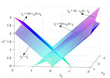
(a) Conditions (A.6) and (B.7).

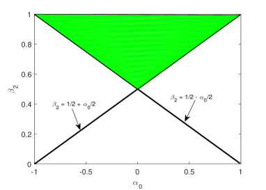
(b) Conditions (A.6), (B.7), and $\beta_{0}=0$.

Figure B.1: The region of the parameters $\alpha_{0},\beta_{0}$, and $\beta_{2}$.

Appendix C De-aliasing in FFT by zero-padding

This appendix introduces the de-aliasing by zero-padding for the cubic term when the Fourier pseudo-spectral method is used for the spatial discretization of the semi-discrete-in-time SAV-GL scheme (LABEL:3.1.6) in our numerical experiments on the Allen-Cahn, the Cahn-Hilliard and the phase field crystal models in Section 3.

Let $N$ be an even integer and $\widehat{\mbox{\boldmath\small$u$}}=(\widehat{u}_{k,l})_{N\times N}$ be the discrete Fourier coefficients of $\mbox{\boldmath\small$u$}=(u_{i,j})_{N\times N}$, and define $\mbox{\boldmath\small$w$}=(w_{i,j})_{N\times N}$ with $w_{i,j}=u_{i,j}^{3}$. Suppose $\widehat{\mbox{\boldmath\small$w$}}=(\widehat{w}_{k,l})_{N\times N}$ is the discrete Fourier coefficients of $w$, then a simple calculation shows that

$$\widehat{w}_{k,l}=\frac{1}{N^{4}}\sum_{(m,n),(p,q)\in\widehat{\mathbb{S}}_{N}}\widehat{u}_{m,n}\widehat{u}_{p,q}\widehat{u}_{k-m-p,l-n-q}$$

$$=\; \frac{1}{N^{4}}\underset{(k-m-p,l-n-q)\in\widehat{\mathbb{S}}_{N}}{\sum_{(m,n),(p,q)\in\widehat{\mathbb{S}}_{N}}}\widehat{u}_{m,n}\widehat{u}_{p,q}\widehat{u}_{k-m-p,l-n-q}+\frac{1}{N^{4}}\underset{(k-m-p,l-n-q)\notin\widehat{\mathbb{S}}_{N}}{\sum_{(m,n),(p,q)\in\widehat{\mathbb{S}}_{N}}}\widehat{u}_{m,n}\widehat{u}_{p,q}\widehat{u}_{k-m-p,l-n-q}.$$ (C.1)

The second summation on the right hand side of (C) is called the aliasing error, and it can be observed that the modes with wave number $k-m-p>\frac{N}{2}$ or $l-n-q>\frac{N}{2}$ are aliased to those with $k-m-p-N$ or $l-n-q-N$, while the modes with wave number $k-m-p<-\frac{N}{2}+1$ or $l-n-q<-\frac{N}{2}+1$ are aliased to those with $k-m-p+N$ or $l-n-q+N$.

The importance of eliminating the aliasing errors, called de-aliasing, has been studied by Orszag [36]. Here, we consider the zero-padding, see e.g. [8, §3.4.2], whose main idea is to use the discrete inverse Fourier transform for $\breve{\mbox{\boldmath\small$u$}}=(\breve{u}_{k,l})_{K\times K}$ instead of $\widehat{\mbox{\boldmath\small$u$}}=(\widehat{u}_{m,n})_{N\times N}$, where $K>N$ is an undetermined number, and $\breve{\mbox{\boldmath\small$u$}}$ is defined by zero padding as follows

$$\breve{u}_{k,l}=\begin{cases}\widehat{u}_{k,l},~{}~{}~{}(k,l)\in\widehat{\mathbb{S}}_{N},\\ 0,~{}~{}~{}~{}~{}~{}\mbox{otherwise}.\end{cases}$$

If letting $\widetilde{\mbox{\boldmath\small$u$}}=(\widetilde{u}_{i,j})_{K\times K}$ be the inverse Fourier transform of $\breve{\mbox{\boldmath\small$u$}}$, defining $\widetilde{\mbox{\boldmath\small$w$}}=(\widetilde{w}_{i,j})_{K\times K}$ with $\widetilde{w}_{i,j}=\widetilde{u}_{i,j}^{3}$, and computing the discrete Fourier coefficients of $\widetilde{\mbox{\boldmath\small$w$}}$ by

$$\breve{w}_{k,l}:=\frac{1}{K^{4}}\!\!\underset{(k-m-p,l-n-q)\in\widehat{\mathbb{S}}_{K}}{\sum_{(m,n),(p,q)\in\widehat{\mathbb{S}}_{K}}}\!\!\!\breve{u}_{m,n}\breve{u}_{p,q}\breve{u}_{k-m-p,l-n-q}+\frac{1}{K^{4}}\!\!\underset{(k-m-p,l-n-q)\notin\widehat{\mathbb{S}}_{K}}{\sum_{(m,n),(p,q)\in\widehat{\mathbb{S}}_{K}}}\!\!\!\breve{u}_{m,n}\breve{u}_{p,q}\breve{u}_{k-m-p,l-n-q},$$ (C.2)

then one can choose the smallest $K>N$ such that the second summation on the right-hand side of (C.2) vanishes for $(k,l)\in\widehat{\mathbb{S}}_{N}$, and then the de-aliased discrete Fourier coefficients of $\mbox{\boldmath\small$w$}=(u_{i,j}^{3})$ are derived by

$$\widehat{w}_{k,l}^{\text{\tiny De}}=\left(\frac{K}{N}\right)^{4}\breve{w}_{k,l},~{}~{}~{}(k,l)\in\widehat{\mathbb{S}}_{N}.$$

It can be observed that the de-aliased coefficients $\widehat{w}_{k,l}^{\text{\tiny De}},~{}(k,l)\in\widehat{\mathbb{S}}_{N}$ is equivalent to the first summation on the right hand side of (C).

The remaining issue is how to determine $K$. In order to make the second summation on the right-hand side of (C.2) to be zero, one needs $\breve{u}_{m,n}\breve{u}_{p,q}\breve{u}_{k-m-p,l-n-q}=0$ for any $(m,n),(p,q)\in\widehat{\mathbb{S}}_{K}$ and $(k-m-p,l-n-q)\notin\widehat{\mathbb{S}}_{K}$. Let $\widehat{\mathbb{S}}_{KN}=\{(k,l)\in\mathbb{Z}^{2}|(k,l)\in\widehat{\mathbb{S}}_{K}~{}\mbox{and}~{}(k,l)\notin\widehat{\mathbb{S}}_{N}\}$. It is obvious that $\breve{u}_{m,n}\breve{u}_{p,q}\breve{u}_{k-m-p,l-n-q}=0$ for $(m,n)\in\widehat{\mathbb{S}}_{KN}$ or $(p,q)\in\widehat{\mathbb{S}}_{KN}$. Hence, one only needs to consider the indexes $(m,n)\in\widehat{\mathbb{S}}_{N}$ and $(p,q)\in\widehat{\mathbb{S}}_{N}$. In that case, the modes $\breve{u}_{m,n}$ and $\breve{u}_{p,q}$ usually are not zero so that it requires $\breve{u}_{k-m-p,l-n-q}=0$ for $(k-m-p,l-n-q)\notin\widehat{\mathbb{S}}_{K}$. Consequently, when the wave number $k-m-p>\frac{K}{2}$ or $l-n-q>\frac{K}{2}$, one needs $k-m-p-K<-\frac{N}{2}+1$ and $l-n-q-K<-\frac{N}{2}+1$, since the modes with $k-m-p>\frac{K}{2}$ or $l-n-q>\frac{K}{2}$ are aliased to those with $k-m-p-K$ or $l-n-q-K$. The largest possible value of $k-m-p$ and $l-n-q$ is $\frac{3}{2}N-2$, and thus the inequality $\frac{3}{2}N-2-K<-\frac{N}{2}+1$ gives $K>2N-3$. In a similar way, when the wave number $k-m-p<-\frac{K}{2}+1$ or $l-n-q<-\frac{K}{2}+1$, it requires $k-m-p+K>\frac{N}{2}$ and $l-n-q+K>\frac{N}{2}$ such that the modes with those wave numbers are zero. Since the smallest possible value of $k-m-p$ and $l-n-q$ is $-\frac{3}{2}N+1$, one can deduce $K>2N-1$. In summary, one can take $K=2N$ in actual applications, and the de-aliased discrete Fourier coefficients of ${\mbox{\boldmath\small$w$}=(u_{i,j}^{3})}$ with zero padding are computed as follows:

(1)

For given 2D vector $\mbox{\boldmath\small$u$}=(u_{i,j})_{N\times N}$, compute the discrete Fourier coefficients $\widehat{\mbox{\boldmath\small$u$}}$ by the FFT;

(2)

Extend $\widehat{\mbox{\boldmath\small$u$}}$ to $\breve{\mbox{\boldmath\small$u$}}$ by zero padding with $K=2N$, perform the inverse Fourier transform of $\breve{\mbox{\boldmath\small$u$}}$ to derive $\widetilde{\mbox{\boldmath\small$u$}}$ by the inverse FFT, and then compute $\widetilde{\mbox{\boldmath\small$w$}}=(\widetilde{u}_{i,j}^{3})_{K\times K}$;

(3)

Compute the discrete Fourier coefficients $\breve{\mbox{\boldmath\small$w$}}$ of $\widetilde{\mbox{\boldmath\small$w$}}$ by the FFT, then multiply a scaling factor $\left(\frac{K}{N}\right)^{4}$ and drop the extra wave numbers to obtain $\widehat{\mbox{\boldmath\small$w$}}^{\text{\tiny De}}$, the de-aliased discrete Fourier coefficients of $\mbox{\boldmath\small$w$}=(u_{i,j}^{3})$.

Several numerical examples in Section 3 will be given to demonstrate the effectiveness of the above de-aliasing procedure. Moreover, such de-aliasing by zero-padding can be easily extended to a general polynomial nonlinear term $u^{p}$, $p\geq 3$, by setting $K=\frac{p+1}{2}N$ and the scaling factor in step (3) as $\left(\frac{K}{N}\right)^{2(p-1)}$, where $2$ in the exponent is the spatial dimension.

Appendix D Estimating the time stepsize for the SAV-GL scheme

This appendix estimates the time stepsize of the SAV-GL scheme (LABEL:3.1.6) with the Fourier pseudo-spectral spatial discretization with the help of the following test equation

$$u^{\prime}(t)=\xi u(t)+\zeta u(t),$$ (D.1)

where $\xi<0$, $|\zeta|\leq|\xi|$. Applying (2.3)-(2.5) to (D.1) yields the semi-implicit scheme

$$\frac{1}{1\!-\!\alpha_{0}}u_{n+1}-\frac{1\!+\!\alpha_{0}}{1\!-\!\alpha_{0}}u_{n}+\frac{\alpha_{0}}{1\!-\!\alpha_{0}}u_{n-1}=\bar{\xi}\left[\frac{\beta_{2}}{1\!-\!\alpha_{0}}u_{n+1}+\frac{\beta_{1}}{1\!-\!\alpha_{0}}u_{n}+\frac{\beta_{0}}{1\!-\!\alpha_{0}}u_{n-1}\right]$$

$$\hskip 56.9055pt+\bar{\zeta}\left[\frac{1\!-\!\alpha_{0}\!+\!\beta_{2}\!-\!\beta_{0}}{1\!-\!\alpha_{0}}u_{n}-\frac{\beta_{2}\!-\!\beta_{0}}{1\!-\!\alpha_{0}}u_{n-1}\right],$$ (D.2)

where $\bar{\xi}=\xi\tau$, $\bar{\zeta}=\zeta\tau$, the parameters $\alpha_{0},\beta_{0}$ and $\beta_{2}$ are assumed to satisfy (A.6). It is known that (D) is stable iff all roots of the characteristic polynomial defined by

$$\mathbb{Q}(x)\!=\!\!\left[\frac{1}{1\!-\!\alpha_{0}}\!-\!\frac{\beta_{2}}{1\!-\!\alpha_{0}}\bar{\xi}\right]\!x^{2}\!-\!\!\left[\frac{1\!+\!\alpha_{0}}{1\!-\!\alpha_{0}}\!+\!\frac{\beta_{1}}{1\!-\!\alpha_{0}}\bar{\xi}\!+\!\!\frac{1\!-\!\alpha_{0}\!+\!\beta_{2}\!-\!\beta_{0}}{1\!-\!\alpha_{0}}\!\bar{\zeta}\right]\!x\!+\!\frac{\alpha_{0}}{1\!-\!\alpha_{0}}\!-\!\frac{\beta_{0}}{1\!-\!\alpha_{0}}\bar{\xi}\!+\!\frac{\beta_{2}\!-\!\beta_{0}}{1\!-\!\alpha_{0}}\bar{\zeta}.$$

are smaller or equal to one in modulus. In order to make sure the roots of $\mathbb{Q}(x)$ are smaller or equal to one in modulus, one requires

$$\begin{aligned} &\left|\alpha_{0}-\beta_{0}\bar{\xi}+\left(\beta_{2}-\beta_{0}\right)\bar{\zeta}\right|\leq\left|1-\beta_{2}\bar{\xi}\right|,\\ &\left|1+\alpha_{0}+\beta_{1}\bar{\xi}+\left(1-\alpha_{0}+\beta_{2}-\beta_{0}\right)\bar{\zeta}\right|\leq\left|1+\alpha_{0}-\left(\beta_{0}+\beta_{2}\right)\bar{\xi}+\left(\beta_{2}-\beta_{0}\right)\bar{\zeta}\right|,\end{aligned}$$

which is equivalent to

$$\begin{aligned} &1\!+\!\alpha_{0}\!-\!\left(\beta_{0}\!+\!\beta_{2}\right)\bar{\xi}\!+\!\left(\beta_{2}\!-\!\beta_{0}\right)\bar{\zeta}\geq 0,~{}~{}1\!-\!\alpha_{0}\!+\!\left(\beta_{0}\!-\!\beta_{2}\right)\bar{\xi}\!-\!\left(\beta_{2}\!-\!\beta_{0}\right)\bar{\zeta}\geq 0,\\[3.0pt] &2(1\!+\!\alpha_{0})\!+\!\left(\beta_{1}\!-\!\beta_{0}\!-\!\beta_{2}\right)\bar{\xi}\!+\!\left(1\!-\!\alpha_{0}\!+\!2\beta_{2}\!-\!2\beta_{0}\right)\bar{\zeta}\!\geq\!0,~{}\!-\!\left(\beta_{1}\!+\!\beta_{0}\!+\!\beta_{2}\right)\bar{\xi}\!-\!\left(1\!-\!\alpha_{0}\right)\bar{\zeta}\!\geq\!0.\end{aligned}$$ (D.3)

Thus, the boundary of the stability region of (D) can be represented by the curves $1\!+\!\alpha_{0}\!-\!\left(\beta_{0}\!+\!\beta_{2}\right)\bar{\xi}\!+\!\left(\beta_{2}\!-\!\beta_{0}\right)\bar{\zeta}=0$, $1\!-\!\alpha_{0}\!+\!\left(\beta_{0}\!-\!\beta_{2}\right)\bar{\xi}\!-\!\left(\beta_{2}\!-\!\beta_{0}\right)\bar{\zeta}=0$, $2(1\!+\!\alpha_{0})\!+\!\left(\beta_{1}\!-\!\beta_{0}\!-\!\beta_{2}\right)\bar{\xi}\!+\!\left(1\!-\!\alpha_{0}\!+\!2\beta_{2}\!-\!2\beta_{0}\right)\bar{\zeta}=0$ and $-\!\left(\beta_{1}\!+\!\beta_{0}\!+\!\beta_{2}\right)\bar{\xi}\!-\!\left(1\!-\!\alpha_{0}\right)\bar{\zeta}=0$.

Next, we discuss two special cases.

$\bullet$ When $\alpha_{0}=\beta_{0}=0$ and $\beta_{2}\geq\frac{1}{2}$, the condition (D.3) reduces to

$$1\!-\!\beta_{2}\bar{\xi}\!+\!\beta_{2}\bar{\zeta}\geq 0,~{}~{}~{}1\!-\!\beta_{2}\bar{\xi}\!-\!\beta_{2}\bar{\zeta}\geq 0,~{}~{}~{}2\!+\!\left(1\!-\!2\beta_{2}\right)\bar{\xi}\!+\!\left(1\!+\!2\beta_{2}\right)\bar{\zeta}\!\geq\!0,~{}~{}~{}\bar{\xi}+\bar{\zeta}\!\leq\!0.$$ (D.4)

Since $\xi<0$ and $|\zeta|\leq|\xi|$, the latter two inequalities imply the first two inequalities in (D.4), so that the boundary of the stability regions of (D) is determined by the curves $2\!+\!\left(1\!-\!2\beta_{2}\right)\bar{\xi}\!+\!\left(1\!+\!2\beta_{2}\right)\bar{\zeta}=0$ and $\bar{\xi}+\bar{\zeta}=0$. Figure D.1 gives the stability regions of (D) with $(\alpha_{0},\beta_{0},\beta_{2})=(0,0,1)$ and $(0,0,2)$. One can deduce that the scheme (D) is unconditionally stable when $\xi<0$ and $\frac{2\beta_{2}-1}{2\beta_{2}+1}\xi\leq\zeta<|\xi|$, and is stable under the time stepsize condition $\tau<\frac{2}{(2\beta_{2}-1)\xi-(2\beta_{2}+1)\zeta}$ when $\xi<0$ and $\zeta<\frac{2\beta_{2}-1}{2\beta_{2}+1}\xi$.

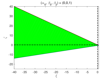
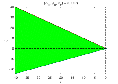
Figure D.1: Stability regions (in green) of (D) for $(\alpha_{0},\beta_{0},\beta_{2})=(0,0,1)$ and $(0,0,2)$.

$\bullet$ When $\beta_{2}=\frac{1+\alpha_{0}}{2}+\beta_{0}$, $\alpha_{0}$ and $\beta_{0}$ are not zero simultaneously, and $-1\leq\alpha_{0}<1$ and $2\beta_{2}+\alpha_{0}\geq 0$, the condition (D.3) reduces to

$$\begin{aligned} &2(1\!+\!\alpha_{0})-(4\beta_{0}\!+\!\alpha_{0}\!+\!1)\bar{\xi}+(1\!+\!\alpha_{0})\bar{\zeta}\geq 0,~{}~{}~{}2(1\!-\!\alpha_{0})-(1\!+\!\alpha_{0})\bar{\xi}-(1\!+\!\alpha_{0})\bar{\zeta}\geq 0,\\[3.0pt] &1+\alpha_{0}-(2\beta_{0}\!+\!\alpha_{0})\bar{\xi}+\bar{\zeta}\geq 0,~{}~{}~{}\bar{\xi}+\bar{\zeta}\leq 0.\end{aligned}$$ (D.5)

Since $\xi<0$ and $|\zeta|\leq|\xi|$, a direct check shows that the boundary of the stability region of (D) can be represented only by the curves $1+\alpha_{0}-(2\beta_{0}\!+\!\alpha_{0})\bar{\xi}+\bar{\zeta}=0$ and $\bar{\xi}+\bar{\zeta}=0$. Figure D.2 gives the stability regions of (D) with $(\alpha_{0},\beta_{0},\beta_{2})=(-1/3,5/12,3/4),(1/3,0,1),(-1/3,1/6,1/2)$ and $(1/3,-1/6,1/2)$, from which one can see that the stability region of (D) with $2\beta_{0}+\alpha_{0}\neq 0$ is much larger than that with $2\beta_{0}+\alpha_{0}=0$, so that the scheme (D) with $2\beta_{0}+\alpha_{0}\neq 0$ possesses better stability properties. More specifically, for (D) with $2\beta_{0}+\alpha_{0}=0$, the upper and lower boundaries of the stability region are determined by the curves $\bar{\zeta}=-\bar{\xi}$ and $\bar{\zeta}=-(1+\alpha_{0})$, respectively. Therefore, (D) with $2\beta_{0}+\alpha_{0}=0$ is unconditionally stable when $\xi<0$ and $0\leq\zeta<|\xi|$, and is stable under the time stepsize condition $\tau<-\frac{1+\alpha_{0}}{\zeta}$ when $\xi<0$ and $\zeta<0$. For (D) with $2\beta_{0}+\alpha_{0}\neq 0$, the upper and lower boundaries of the stability region are the curves $\bar{\zeta}=-\bar{\xi}$ and $\bar{\zeta}=(2\beta_{0}\!+\!\alpha_{0})\bar{\xi}-(1\!+\!\alpha_{0})$, respectively. Therefore, (D) with $2\beta_{0}+\alpha_{0}\neq 0$ is unconditionally stable when $\xi<0$ and $(2\beta_{0}\!+\!\alpha_{0})\xi\leq\zeta<|\xi|$, and is stable under the condition $\tau<\frac{1+\alpha_{0}}{(2\beta_{0}+\alpha_{0})\xi-\zeta}$ when $\xi<0$ and $\zeta<(2\beta_{0}\!+\!\alpha_{0})\xi$.

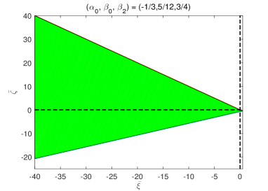
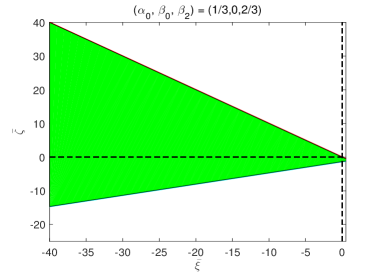
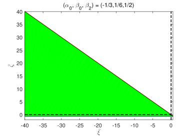
Figure D.2: Stability regions of the scheme (D) with $(\alpha_{0},\beta_{0},\beta_{2})=(-1/3,5/12,3/4)$, $(1/3,0,1)$, $(-1/3,1/6,1/2)$ and $(1/3,-1/6,1/2)$.

References

- [1] D.M. Anderson, G.B. McFadden, and A.A. Wheeler, Diffuse-interface methods in fluid mechanics, Annu. Rev. Fluid Mech., 30(1998), 139–165.
- [2] S.M. Allen and J.W. Cahn, A microscopic theory for antiphase boundary motion and its application to antiphase domain coarsening, Acta. Metall., 27(1979), 1085–1095.
- [3] G. Akrivis, B.Y. Li, and D.F. Li, Energy-decaying extrapolated RK-SAV methods for the Allen-Cahn and Cahn-Hilliard equations, SIAM J. Sci. Comput., 41(2019), A3703–A3727.
- [4] S. Badia, F. Guilln-Gonzlez, and J.V. Gutirrez-Santacreu, Finite element approximation of nematic liquid crystal flows using a saddle-point structure, J. Comput. Phys., 230(2011), 1686–1706.
- [5] J. Berry, M. Grant, and K.R. Elder, Diffusive atomistic dynamics of edge dislocations in two dimensions, Phys. Rev. E, 73(2006), 031609.
- [6] J.W. Cahn and J.E. Hilliard, Free energy of a nonunifotm ststem. I: Interfacial free energy, J. Chem. Phys., 28(1958), 258–267.
- [7] M. Calvo and T. Grande, On the asymptotic stability of -methds for delay differential equations, Numer. Math., 54(1988), 257–269.
- [8] C. Canuto, M.Y. Hussaini, A. Quarteroni, and T.A. Zang, Spectral Methods: Fundamentals in Single Domains, Springer, 2006.
- [9] W.B. Chen, S. Conde, C. Wang, X.M. Wang, and S.M. Wise, A linear energy stable scheme for a thin film model without slope selection, J. Sci. Comput., 52(2012), 546–562.
- [10] Q. Cheng and J. Shen, Multiple scalar auxilary variable (MSAV) approach and its application to the phase-field vesicle membrane model, SIAM J. Sci. Comput., 40(2018), A3982–A4006.
- [11] Q. Cheng, J. Shen, and X.F. Yang, Highly efficient and accurate numerical schemes for the epitaxial thin film growth models by using the SAV approach, J. Sci. Comput., 78(2019), 1467–1487.
- [12] Q. Cheng, The generalized scalar auxiliary variable approach (G-SAV) for gradient flows, arXiv. 2002.00236, 2020.
- [13] G. Dahlquist, Error analysis for a class of methods for stiff nonlinear initial value problems, in: G.A. Watson, Numerical Analysis, Lecture Notes in Mathematics, vol. 506, Springer, 1976, 60–72.
- [14] Q. Du, L.L. Ju, X. Li, and Z.H. Qiao, Maximum principle preserving exponential time differencing schemes for the nonlocal Allen-Cahn equation, SIAM J. Numer. Anal., 57(2019), 875–898,
- [15] K.R. Elder, M. Katakowski, M. Haataja, and M. Grant, Modeling elasticity in crystal growth, Phys. Rev. Lett., 88(2002), 245701.
- [16] C.M. Elliott and A.M. Stuart, The global dynamics of discrete semilinear parabolic equations, SIAM J. Numer. Anal., 30(1993), 1622–1663.
- [17] D.J. Eyre, Unconditionally gradient stable time marching the Cahn-Hilliard equation, Mater. Res. Soc. Symp. Proc., 529(1998), 39–46.
- [18] J.G.E.M. Fraaije, Dynamic density functional theory for microphase separation kinetics of block copolymer melts, J. Chem. Phys., 99(1993), 9202–9212.
- [19] J.G.E.M. Fraaije and G.J.A. Sevink, Model for pattern formation in polymer surfactant nanodroplets, Macromolecules, 36(2003), 7891–7893.
- [20] D. Gottlieb and S.A. Orszag, Numerical Analysis of Spectral Methods: Theory and Applications, SIAM, 1977.
- [21] S. Gottlieb and C. Wang, Stability and convergence analysis of fully discrete Fourier collocation spectral method for 3-D viscous Burgers’ equation, J. Sci. Comput., 53(2012), 102–128.
- [22] Y.Z. Gong, J. Zhao, and Q. Wang, Arbitrarily high-order unconditionally energy stable SAV schemes for gradient flow models, Comput. Phys. Commun., 249(2020), 107033.
- [23] F. Guilln-Gonzlez and G. Tierra, On linear schemes for a Cahn-Hilliard diffuse interface model, J. Comput. Phys., 234(2013), 140–171.
- [24] E. Hairer and G. Wanner, Solving Ordinary Differential Equations II: Stiff and Differential-Algebraic Problems, 2nd ed., Springer, New York, 1996.
- [25] D.M. Hou, M. Azaiez, and C.J. Xu, A variant of scalar auxiliary variable approaches for gradient flows, J. Comput. Phys., 395(2019), 307–332.
- [26] F.K. Huang, J. Shen, and Z.G. Yang, A highly efficient and accurate new scalar auxiliary variable approach for gradient flows, SIAM J. Sci. Comput., 42(2020), A2514–A2536.
- [27] F.K. Huang and J. Shen, A new class of implicit-explicit BDF SAV schemes for general dissipative systems and their error analysis, Comput. Methods Appl. Mech. Engrg., 392(2022), 114718.
- [28] M.S. Jiang, Z.Y. Zhang, and J. Zhao, Improving the accuracy and consistency of the scalar auxiliary variable (SAV) method with relaxation, J. Comput. Phys., 456(2022), 110954.
- [29] L.L. Ju, X. Li, Z.H. Qiao, and H. Zhang, Energy stability and error estimates of exponential time differencing schemes for the epitaxial growth model without slope selection, Math. Comput., 87(2018), 1859–1885.
- [30] A. Karma and M. Plapp, Spiral surface growth without desorption, Phys. Rev. Lett., 81(1998), 4444–4452.
- [31] R.G. Larson, Arrested tumbling in shearing flows of liquid crystal polymers, Macromolecules, 23(1990), 3983–3992.
- [32] F.M. Leslie, Theory of flow phenomena in liquid crystals, Adv. Liquid Cryst., 4(1979), 1–81.
- [33] Z.G. Liu and X.L. Li, The exponential scalar auxilary variable (E-SAV) approach for phase field models and its explicit computing, SIAM J. Sci. Comput., 42(2020), B630–B655.
- [34] Z.G. Liu and X.L. Li, A highly efficient and accurate exponential semi-implicit scalar auxiliary variable (ESI-SAV) approach for dissipative system, J. Comput. Phys., 447(2021), 110703.
- [35] J.T. Oden, A. Hawkins, and S. Prudhomme, General diffuse-interface theories and an approach to predictive tumor growth modeling, Math. Models Meth. Appl. Sci., 20(2010), 477–517.
- [36] S.A. Orszag, Elimination of aliasing in finite-difference schemes by filtering high wavenumber components, J. Atmospheric Sci., 28 (1971), 1074.
- [37] J. Shen and X.F. Yang, Numerical approximations of Allen-Cahn and Cahn-Hilliard equations, Dis. & Contin. Dyn. Sys., 28(2010), 1669–1691.
- [38] J. Shen, T. Tang, and L.L. Wang, Spectral Methods: Algorithms, Analysis and Applications, Springer, 2011.
- [39] J. Shen, C. Wang, X.M. Wang, and S.M. Wise, Second-order convex splitting schemes for gradient flows with Ehrlich-Schwoebel type energy: Application to thin film epitaxy, SIAM J. Numer. Anal., 50(2012), 105–125.
- [40] J. Shen, J. Xu, and J. Yang, The scalar auxiliary variable (SAV) approach for gradient flows, J. Comput. Phys., 395(2018), 407–416.
- [41] J. Shen and J. Xu, Convergence and error analysis for the scalar auxiliary variable (SAV) schemes to gradient flows, SIAM J. Numer. Anal., 56(2018), 2895–2912.
- [42] J. Shen, J. Xu, and J. Yang, A new class of efficient and robust energy stable schemes for gradient flows, SIAM Rev., 61(2019), 474–506.
- [43] E. Tadmor, Stability analysis of finite-difference, pseudospectral and Fourier-Galerkin approximations for time-dependent problems, SIAM Rev., 29(1987), 525–555.
- [44] Z.Q. Tan and H.Z. Tang, A general class of linear unconditionally energy stable schemes for the gradient flows. I. Comput.Phys., 464(2022), 111372.
- [45] C.J. Xu and T. Tang, Stability analysis of large time-stepping methods for epitaxial growth models, SIAM J. Numer. Anal., 44(2006), 1759–1779.
- [46] Y.U. Wang, Y.M. Jin, and A.G. Khachaturyan, Phase field microelasticity modeling of dislocation dynamics near free surface and in heteroepitaxial thin films, Acta Mater., 51(2003), 4209–4223.
- [47] L. Wang and H.J. Yu, On efficient second order stabilized semi-implicit schemes for the Cahn-Hilliard phase-field equation, J. Sci. Comput., 77(2018), 1185–1209.
- [48] X.Q. Wang, L.L. Ju, and Q. Du, Efficient and stable exponential time differencing Runge-Kutta methods for phase field elastic bending energy models, J. Comput. Phys., 316(2016), 21–38.
- [49] S.M. Wise, J.S. Lowengrub, H.B. Frieboes, and V. Cristini, Three-dimensional multispecies nonlinear tumor growth-I: model and numerical method, J. Theor. Biol., 253(2008), 524–543.
- [50] K.A. Wu, A. Adland, and A. Karma, Phase-field-crystal model for fcc ordering, Phys. Rev. E, 81(2010), 061601.
- [51] X.F. Yang, Linear, first and second-order, unconditionally energy stable numerical schemes for the phase field model of homopolymer blends, J. Comput. Phys., 327(2016), 294–316.
- [52] X.F. Yang, J. Zhao, Q. Wang, and J. Shen, Numerical approximations for a three components Cahn-Hilliard phase-field model based on the invariant energy quadratization method, Math. Models Meth. Appl. Sci., 27(2017), 1993–2030.
- [53] X.F. Yang and L.L. Ju, Efficient linear schemes with unconditional energy stability for the phase field elastic bending energy model, Comput. Meth. Appl. Mech. Eng., 315(2017), 691–712.
- [54] Z.G. Yang, L.L. Lin, and S.C. Dong, A family of second-order energy-stable schemes for Cahn-Hilliard type equations, J. Comput. Phys., 383(2019), 24–54.
- [55] X.F. Yang and G.D. Zhang, Convergence analysis for the invarint energy quadratization (IEQ) schemes for solving the Cahn-Hilliard and Allen-Cahn equations with general nonlinear potential, J. Sci. Comput., 82(2020), 55.
- [56] J.X. Yang and J. Kim, A variant of stabilized-scalar auxiliary variable (S-SAV) approach for a modified phase-field surfactant model, Comput. Phys. Commun., 261(2021), 107825.
- [57] P.T. Yue, J.J. Feng, C. Liu, and J. Shen, A diffuse-interface method for simulating two-phase flows of complex fluids, J. Fluid Mech., 515(2004), 293–317.
- [58] Y.R. Zhang and J. Shen, A generalized SAV approach with relaxation for dissipative systems, J. Comput. Phys., 464(2022), 111311.