Flat Seeking Bayesian Neural Networks

Abstract

Bayesian Neural Networks (BNNs) provide a probabilistic interpretation for deep learning models by imposing a prior distribution over model parameters and inferring a posterior distribution based on observed data. The model sampled from the posterior distribution can be used for providing ensemble predictions and quantifying prediction uncertainty. It is well-known that deep learning models with lower sharpness have better generalization ability. However, existing posterior inferences are not aware of sharpness/flatness in terms of formulation, possibly leading to high sharpness for the models sampled from them. In this paper, we develop theories, the Bayesian setting, and the variational inference approach for the sharpness-aware posterior. Specifically, the models sampled from our sharpness-aware posterior, and the optimal approximate posterior estimating this sharpness-aware posterior, have better flatness, hence possibly possessing higher generalization ability. We conduct experiments by leveraging the sharpness-aware posterior with state-of-the-art Bayesian Neural Networks, showing that the flat-seeking counterparts outperform their baselines in all metrics of interest.

1 Introduction

Bayesian Neural Networks (BNNs) provide a way to interpret deep learning models probabilistically. This is done by setting a prior distribution over model parameters and then inferring a posterior distribution over model parameters based on observed data. This allows us to not only make predictions, but also quantify prediction uncertainty, which is useful for many real-world applications. To sample deep learning models from complex and complicated posterior distributions, advanced particle-sampling approaches such as Hamiltonian Monte Carlo (HMC) [41], Stochastic Gradient HMC (SGHMC) [10], Stochastic Gradient Langevin dynamics (SGLD) [59], and Stein Variational Gradient Descent (SVGD) [36] are often used. However, these methods can be computationally expensive, particularly when many models need to be sampled for better ensembles.

To alleviate this computational burden and enable the sampling of multiple deep learning models from posterior distributions, variational inference approaches employ approximate posteriors to estimate the true posterior. These methods utilize approximate posteriors that belong to sufficiently rich families, which are both economical and convenient to sample from. However, the pioneering works in variational inference, such as [21, 5, 33], assume approximate posteriors to be fully factorized distributions, also known as mean-field variational inference. This approach fails to account for the strong statistical dependencies among random weights of neural networks, limiting its ability to capture the complex structure of the true posterior and estimate the true model uncertainty. To overcome this issue, latter works have attempted to provide posterior approximations with richer expressiveness [62, 52, 53, 55, 20, 45, 56, 30, 48]. These approaches aim to improve the accuracy of the posterior approximation and enable more effective uncertainty quantification.

In the context of standard deep network training, it has been observed that flat minimizers can enhance the generalization capability of models. This is achieved by enabling them to locate wider local minima that are more robust to shifts between train and test sets. Several studies, including [27, 47, 15], have shown evidence to support this principle. However, the posteriors used in existing Bayesian neural networks (BNNs) do not account for the sharpness/flatness of the models derived from them in terms of model formulation. As a result, the sampled models can be located in regions of high sharpness and low flatness, leading to poor generalization ability. Moreover, in variational inference methods, using approximate posteriors to estimate these non-sharpness-aware posteriors can result in sampled models from the corresponding optimal approximate posterior lacking awareness of sharpness/flatness, hence causing them to suffer from poor generalization ability.

In this paper, our objective is to propose a sharpness-aware posterior for learning BNNs, which samples models with high flatness for better generalization ability. To achieve this, we devise both a Bayesian setting and a variational inference approach for the proposed posterior. By estimating the optimal approximate posteriors, we can generate flatter models that improve the generalization ability. Our approach is as follows: In Theorem 3.1, we show that the standard posterior is the optimal solution to an optimization problem that balances the empirical loss induced by models sampled from an approximate posterior for fitting a training set with a Kullback-Leibler (KL) divergence, which encourages a simple approximate posterior. Based on this insight, we replace the empirical loss induced by the approximate posterior with the general loss over the entire data-label distribution in Theorem 3.2 to improve the generalization ability. Inspired by sharpness-aware minimization [16], we develop an upper-bound of the general loss in Theorem 3.2, leading us to formulate the sharpness-aware posterior in Theorem 3.3. Finally, we devise the Bayesian setting and variational approach for the sharpness-aware posterior. Overall, our contributions in this paper can be summarized as follows:

• We propose and develop theories, the Bayesian setting, and the variational inference approach for the sharpness-aware posterior. This posterior enables us to sample a set of flat models that improve the model generalization ability. We note that SAM [16] only considers the sharpness for a single model, while ours is the first work studying the concept and theory of the sharpness for a distribution $\mathbb{Q}$ over models. Additionally, the proof of Theorem 3.2 is very challenging, elegant, and complicated because of the infinite number of models in the support of $\mathbb{Q}$.

• We conduct extensive experiments by leveraging our sharpness-aware posterior with the state-of-the-art and well-known BNNs, including BNNs with an approximate Gaussian distribution [33], BNNs with stochastic gradient Langevin dynamics (SGLD) [59], MC-Dropout [18], Bayesian deep ensemble [35], and SWAG [39] to demonstrate that the flat-seeking counterparts consistently outperform the corresponding approaches in all metrics of interest, including the ensemble accuracy, expected calibration error (ECE), and negative log-likelihood (NLL).

2 Related Work

2.1 Bayesian Neural Networks

Markov chain Monte Carlo (MCMC): This approach allows us to sample multiple models from the posterior distribution and was well-known for inference with neural networks through the Hamiltonian Monte Carlo (HMC) [41]. However, HMC requires the estimation of full gradients, which is computationally expensive for neural networks. To make the HMC framework practical, Stochastic Gradient HMC (SGHMC) [10] enables stochastic gradients to be used in Bayesian inference, crucial for both scalability and exploring a space of solutions. Alternatively, stochastic gradient Langevin dynamics (SGLD) [59] employs first-order Langevin dynamics in the stochastic gradient setting. Additionally, Stein Variational Gradient Descent (SVGD) [36] maintains a set of particles to gradually approach a posterior distribution. Theoretically, all SGHMC, SGLD, and SVGD asymptotically sample from the posterior in the limit of infinitely small step sizes.

Variational Inference: This approach uses an approximate posterior distribution in a family to estimate the true posterior distribution by maximizing a variational lower bound. [21] suggests fitting a Gaussian variational posterior approximation over the weights of neural networks, which was generalized in [32, 33, 5], using the reparameterization trick for training deep latent variable models. To provide posterior approximations with richer expressiveness, many extensive studies have been proposed. Notably, [38] treats the weight matrix as a whole via a matrix variate Gaussian [22] and approximates the posterior based on this parameterization. Several later works have inspected this distribution to examine different structured representations for the variational Gaussian posterior, such as Kronecker-factored [60, 52, 53], k-tied distribution [55], non-centered or rank-1 parameterization [20, 14]. Another recipe to represent the true covariance matrix of Gaussian posterior is through the low-rank approximation [45, 56, 30, 39].

Dropout Variational Inference: This approach utilizes dropout to characterize approximate posteriors. Typically, [18] and [33] use this principle to propose Bayesian Dropout inference methods such as MC Dropout and Variational Dropout. Concrete dropout [19] extends this idea to optimize the dropout probabilities. Variational Structured Dropout [43] employs Householder transformation to learn a structured representation for multiplicative Gaussian noise in the Variational Dropout method.

2.2 Flat Minima

Flat minimizers have been found to improve the generalization ability of neural networks. This is because they enable models to find wider local minima, which makes them more robust against shifts between train and test sets [27, 47, 15, 44]. The relationship between generalization ability and the width of minima has been investigated theoretically and empirically in many studies, notably [23, 42, 12, 17]. Moreover, various methods seeking flat minima have been proposed in [46, 9, 29, 25, 16, 44]. Typically, [29, 26, 58] investigate the impacts of different training factors such as batch size, learning rate, covariance of gradient, and dropout on the flatness of found minima. Additionally, several approaches pursue wide local minima by adding regularization terms to the loss function [46, 62, 61, 9]. Examples of such regularization terms include softmax output’s low entropy penalty [46] and distillation losses [62, 61].

SAM, a method that aims to minimize the worst-case loss around the current model by seeking flat regions, has recently gained attention due to its scalability and effectiveness compared to previous methods [16, 57]. SAM has been widely applied in various domains and tasks, such as meta-learning bi-level optimization [1], federated learning [51], multi-task learning [50], where it achieved tighter convergence rates and proposed generalization bounds. SAM has also demonstrated its generalization ability in vision models [11], language models [3], domain generalization [8], and multi-task learning [50]. Some researchers have attempted to improve SAM by exploiting its geometry [34, 31], additionally minimizing the surrogate gap [63], and speeding up its training time [13, 37]. Regarding the behavior of SAM, [28] empirically studied the difference in sharpness obtained by SAM [16] and SWA [24], [40] showed that SAM is an optimal Bayes relaxation of the standard Bayesian inference with a normal posterior, while [44] proved that distribution robustness [4, 49] is a probabilistic extension of SAM.

3 Proposed Framework

In what follows, we present the technicality of our proposed sharpness-aware posterior. Particularly, Section 3.1 introduces the problem setting and motivation for our sharpness-aware posterior. Section 3.2 is dedicated to our theory development, while Section 3.3 is used to describe the Bayesian setting and variational inference approach for our sharpness-aware posterior.

3.1 Problem Setting and Motivation

We aim to develop Sharpness-Aware Bayesian Neural Networks (SA-BNN). Consider a family of neural networks $f_{\theta}(x)$ with $\theta\in\Theta$ and a training set $\mathcal{S}=\{(x_{1},y_{1}),...,(x_{n},y_{n})\}$ where $\left(x_{i},y_{i}\right)\sim\mathcal{D}$. We wish to learn a posterior distribution $\mathbb{Q}_{S}^{SA}$ with the density function $q^{SA}(\theta|\mathcal{S})$ such that any model $\theta\sim\mathbb{Q}^{SA}_{S}$ is aware of the sharpness when predicting over the training set $\mathcal{S}$.

We depart with the standard posterior

$$q(\theta\mid\mathcal{S})\propto\prod_{i=1}^{n}p(y_{i}\mid x_{i},\mathcal{S},\theta)p(\theta),$$

where the prior distribution $\mathbb{P}$ has the density function $p(\theta)$ and the likelihood has the form

$$p\left(y\mid x,\mathcal{S},\theta\right) \propto\exp\left\{-\frac{\lambda}{|\mathcal{S}|}\ell\left(f_{\theta}(x),y\right)\right\}=\exp\left\{-\frac{\lambda}{n}\ell\left(f_{\theta}(x),y\right)\right\}$$

with the loss function $\ell$. The standard posterior $\mathbb{Q}_{\mathcal{S}}$ has the density function defined as

$$q(\theta\mid\mathcal{S})\propto\exp\left\{-\frac{\lambda}{n}\sum_{i=1}^{n}\ell\left(f_{\theta}\left(x_{i}\right),y_{i}\right)\right\}p(\theta),$$ (1)

where $\lambda\geq 0$ is a regularization parameter.

We define the general and empirical losses as follows:

$$\mathcal{L}_{\mathcal{D}}\left(\theta\right)=\mathbb{E}_{\left(x,y\right)\sim\mathcal{D}}\left[\ell\left(f_{\theta}\left(x\right),y\right)\right].$$

$$\mathcal{L}_{\mathcal{S}}\left(\theta\right)=\mathbb{E}_{\left(x,y\right)\sim\mathcal{\mathcal{S}}}\left[\ell\left(f_{\theta}\left(x\right),y\right)\right]=\frac{1}{n}\sum_{i=1}^{n}\ell\left(f_{\theta}\left(x_{i}\right),y_{i}\right).$$

Basically, the general loss is defined as the expected loss over the entire data-label distribution $\mathcal{D}$, while the empirical loss is defined as the empirical loss over a specific training set $\mathcal{S}$.

The standard posterior in Eq. (1) can be rewritten as

$$q(\theta\mid\mathcal{S})\propto\exp\left\{-\lambda\mathcal{L}_{\mathcal{S}}\left(\theta\right)\right\}p(\theta).$$ (2)

Given a distribution $\mathbb{Q}$ with the density function $q\left(\theta\right)$ over the model parameters $\theta\in\Theta$, we define the empirical and general losses over this model distribution $\mathbb{Q}$ as

$$\mathcal{L_{S}}\left(\mathbb{Q}\right)=\int_{\Theta}\mathcal{L}_{\mathcal{S}}\left(\theta\right)d\mathbb{Q}\left(\theta\right)=\int_{\Theta}\mathcal{L}_{\mathcal{S}}\left(\theta\right)q\left(\theta\right)d\theta.$$

$$\mathcal{L_{D}}\left(\mathbb{Q}\right)=\int_{\Theta}\mathcal{L}_{\mathcal{D}}\left(\theta\right)d\mathbb{Q}\left(\theta\right)=\int_{\Theta}\mathcal{L}_{\mathcal{D}}\left(\theta\right)q\left(\theta\right)d\theta.$$

Specifically, the general loss over the model distribution $\mathbb{Q}$ is defined as the expectation of the general losses incurred by the models sampled from this distribution, while the empirical loss over the model distribution $\mathbb{Q}$ is defined as the expectation of the empirical losses incurred by the models sampled from this distribution.

3.2 Our Theory Development

We now present the theory development for the sharpness-aware posterior whose proofs can be found in the supplementary material. Inspired by the Gibbs form of the standard posterior $\mathbb{Q}_{\mathcal{S}}$ in Eq. (2), we establish the following theorem to connect the standard posterior $\mathbb{Q}_{\mathcal{S}}$ with the density $q(\theta\mid\mathcal{S})$ and the empirical loss $\mathcal{L_{S}}\left(\mathbb{Q}\right)$ [7, 2].

Theorem 3.1.

Consider the following optimization problem

$$\min_{\mathbb{Q<<\mathbb{P}}}\left\{\lambda\mathcal{L}_{S}\left(\mathbb{Q}\right)+KL\left(\mathbb{Q},\mathbb{P}\right)\right\},$$ (3)

where we search over $\mathbb{Q}$ absolutely continuous w.r.t. $\mathbb{P}$ and $KL\left(\cdot,\cdot\right)$ is the Kullback-Leibler divergence. This optimization has a closed-form optimal solution $\mathbb{Q}^{*}$ with the density

$$q^{*}\left(\theta\right)\propto\exp\left\{-\lambda\mathcal{L}_{\mathcal{S}}\left(\theta\right)\right\}p(\theta),$$

which is exactly the standard posterior $\mathbb{Q}_{\mathcal{S}}$ with the density $q(\theta\mid\mathcal{S})$.

Theorem 3.1 reveals that we need to find the posterior $\mathbb{Q}_{\mathcal{S}}$ balancing between optimizing its empirical loss $\mathcal{L}_{S}\left(\mathbb{Q}\right)$ and simplicity via $KL\left(\mathbb{Q},\mathbb{P}\right)$. However, minimizing the empirical loss $\mathcal{L}_{S}\left(\mathbb{Q}\right)$ only ensures the correct predictions for the training examples in $\mathcal{S}$, hence possibly encountering overfitting. Therefore, it is desirable to replace the empirical loss by the general loss to combat overfitting.

To mitigate overfitting, in (8), we replace the empirical loss by the general loss and solve the following optimization problem (OP):

$$\min_{\mathbb{Q<<\mathbb{P}}}\left\{\lambda\mathcal{L}_{\mathcal{D}}\left(\mathbb{Q}\right)+KL\left(\mathbb{Q},\mathbb{P}\right)\right\}.$$ (4)

Notably, solving the optimization problem (OP) in (4) is generally intractable. To make it tractable, we find its upper-bound which is relevant to the sharpness of a distribution $\mathbb{Q}$ over models as shown in the following theorem.

Theorem 3.2.

Assume that $\Theta$ is a compact set. Under some mild conditions, given any $\delta\in[0;1]$, with the probability at least $1-\delta$ over the choice of $\mathcal{S}\sim\mathcal{D}^{n}$, for any distribution $\mathbb{Q}$, we have

$$\mathcal{L}_{\mathcal{D}}\left(\mathbb{Q}\right)\leq\mathbb{E}_{\theta\sim\mathbb{Q}}\left[\max_{\theta^{\prime}:\left\|\theta^{\prime}-\theta\right\|\leq\rho}\mathcal{L}_{\mathcal{S}}\left(\theta^{\prime}\right)\right]+f\left(\max_{\theta\in\Theta}\left\|\theta\right\|^{2},n\right),$$

where $f$ is a non-decreasing function w.r.t. the first variable and approaches $0$ when the training size $n$ approaches $\infty$.

We note that the proof of Theorem 3.2 is not a trivial extension of sharpness-aware minimization because we need to tackle the general and empirical losses over a distribution $\mathbb{Q}$. To make explicit our sharpness over a distribution $\mathbb{Q}$ on models, we rewrite the upper-bound of the inequality as

$$\mathbb{E}_{\theta\sim\mathbb{Q}}\left[\max_{\theta^{\prime}:\left\|\theta^{\prime}-\theta\right\|\leq\rho}\mathcal{L}_{\mathcal{S}}\left(\theta^{\prime}\right)-\mathcal{L}_{\mathcal{S}}\left(\theta\right)\right]+\mathcal{L}_{\mathcal{S}}\left(\mathbb{Q}\right)+f\left(\max_{\theta\in\Theta}\left\|\theta\right\|^{2},n\right),$$

where the first term $\mathbb{E}_{\theta\sim\mathbb{Q}}\left[\max_{\theta^{\prime}:\left\|\theta^{\prime}-\theta\right\|\leq\rho}\mathcal{L}_{\mathcal{S}}\left(\theta^{\prime}\right)-\mathcal{L}_{\mathcal{S}}\left(\theta\right)\right]$ can be regarded as the sharpness over the distribution $\mathbb{Q}$ on the model space and the last term $f\left(\max_{\theta\in\Theta}\left\|\theta\right\|^{2},n\right)$ is a constant.

Moreover, inspired by Theorem 3.2, we propose solving the following OP which forms an upper-bound of the desirable OP in (4)

$$\min_{\mathbb{Q<<\mathbb{P}}}\left\{\lambda\mathbb{E}_{\theta\sim\mathbb{Q}}\left[\max_{\theta^{\prime}:\left\|\theta^{\prime}-\theta\right\|\leq\rho}\mathcal{L}_{\mathcal{S}}\left(\theta^{\prime}\right)\right]+KL\left(\mathbb{Q},\mathbb{P}\right)\right\}.$$ (5)

The following theorem characterizes the optimal solution of the OP in (5).

Theorem 3.3.

The optimal solution the OP in (5) is the sharpness-aware posterior distribution $\mathbb{Q}_{S}^{SA}$ with the density function $q^{SA}(\theta|\mathcal{S})$:

$$q^{SA}(\theta|\mathcal{S}) \propto\exp\left\{-\lambda\max_{\theta^{\prime}:\left\|\theta^{\prime}-\theta\right\|\leq\rho}\mathcal{L}_{\mathcal{S}}\left(\theta^{\prime}\right)\right\}p\left(\theta\right)=\exp\left\{-\lambda\mathcal{L}_{\mathcal{S}}\left(s\left(\theta\right)\right)\right\}p\left(\theta\right),$$

where we have defined $s\left(\theta\right)=\underset{{}_{\theta^{\prime}:\left\|\theta^{\prime}-\theta\right\|\leq\rho}}{\text{argmax}}\mathcal{L}_{\mathcal{S}}\left(\theta^{\prime}\right)$.

Theorem 3.3 describes the close form of the sharpness-aware posterior distribution $\mathbb{Q}_{S}^{SA}$ with the density function $q^{SA}(\theta|\mathcal{S})$. Based on this characterization, in what follows, we introduce the SA Bayesian setting that sheds lights on its variational approach.

3.3 Sharpness-Aware Bayesian Setting and Its Variational Approach

Bayesian Setting: To promote the Bayesian setting for sharpness-aware posterior distribution $\mathbb{Q}_{S}^{SA}$, we examine the sharpness-aware likelihood

$$p^{SA}\left(y\mid x,\mathcal{S},\theta\right) \propto\exp\left\{-\frac{\lambda}{|\mathcal{S}|}\ell\left(f_{s\left(\theta\right)}(x),y\right)\right\}=\exp\left\{-\frac{\lambda}{n}\ell\left(f_{s\left(\theta\right)}(x),y\right)\right\},$$

where $s\left(\theta\right)=\underset{{}_{\theta^{\prime}:\left\|\theta^{\prime}-\theta\right\|\leq\rho}}{\text{argmax}}\mathcal{L}_{\mathcal{S}}\left(\theta^{\prime}\right)$.

With this predefined sharpness-aware likelihood, we can recover the sharpness-aware posterior distribution $\mathbb{Q}_{S}^{SA}$ with the density function $q^{SA}(\theta|\mathcal{S})$:

$$q^{SA}(\theta|\mathcal{S})\propto\prod_{i=1}^{n}p^{SA}\left(y_{i}\mid x_{i},\mathcal{S},\theta\right)p\left(\theta\right).$$

Variational inference for the sharpness-aware posterior distribution: We now develop the variational inference for the sharpness-aware posterior distribution. Let denote $X=\left[x_{1},...,x_{n}\right]$ and $Y=\left[y_{1},...,y_{n}\right]$. Considering an approximate posterior family $\left\{q_{\phi}\left(\theta\right):\phi\in\Phi\right\}$, we have

$$\log p^{SA}\left(Y\mid X,\mathcal{S}\right)=\int_{\Theta}q_{\phi}\left(\theta\right)\log p^{SA}\left(Y\mid X,\mathcal{S}\right)d\theta$$

$$=\int_{\Theta}q_{\phi}\left(\theta\right)\log\frac{p^{SA}\left(Y\mid\theta,X,\mathcal{S}\right)p\left(\theta\right)}{q_{\phi}\left(\theta\right)}\frac{q_{\phi}\left(\theta\right)}{q^{SA}(\theta|\mathcal{S})}d\theta$$

$$=\mathbb{E}_{q_{\phi}\left(\theta\right)}\left[\sum_{i=1}^{n}\log p^{SA}\left(y_{i}\mid x_{i},\mathcal{S},\theta\right)\right]-KL\left(q_{\phi},p\right)+KL\left(q_{\phi},q^{SA}\right).$$

It is obvious that we need to maximize the following lower bound for maximally reducing the gap $KL\left(q_{\phi},q^{SA}\right)$:

$$\max_{q_{\phi}}\left\{\mathbb{E}_{q_{\phi}\left(\theta\right)}\left[\sum_{i=1}^{n}\log p^{SA}\left(y_{i}\mid x_{i},\mathcal{S},\theta\right)\right]-KL\left(q_{\phi},p\right)\right\},$$

which can be equivalently rewritten as

$$\min_{q_{\phi}}\left\{\lambda\mathbb{E}_{q_{\phi}\left(\theta\right)}\left[\mathcal{L}_{\mathcal{S}}\left(s\left(\theta\right)\right)\right]+KL\left(q_{\phi},p\right)\right\}\text{or}$$

$$\min_{q_{\phi}}\left\{\lambda\mathbb{E}_{q_{\phi}\left(\theta\right)}\left[\max_{\theta^{\prime}:\left\|\theta^{\prime}-\theta\right\|\leq\rho}\mathcal{L}_{\mathcal{S}}\left(\theta^{\prime}\right)\right]+KL\left(q_{\phi},p\right)\right\}.$$ (6)

Derivation for Variational Approach with A Gaussian Approximate Posterior: Inspired by the geometry-based SAM approaches  [34, 31], we incorporate the geometry to the SA variational approach via the distance to define the ball for the sharpness as $\left\|\theta^{\prime}-\theta\right\|_{\text{diag}(T_{\theta})}=\sqrt{\left(\theta^{\prime}-\theta\right)^{T}\text{diag}(T_{\theta})^{-1}\left(\theta^{\prime}-\theta\right)}$ as

$$\min_{q_{\phi}}\left\{\lambda\mathbb{E}_{q_{\phi}\left(\theta\right)}\left[\max_{\theta^{\prime}:\left\|\theta^{\prime}-\theta\right\|_{\text{diag}(T_{\theta})}\leq\rho}\mathcal{L}_{\mathcal{S}}\left(\theta^{\prime}\right)\right]+KL\left(q_{\phi},p\right)\right\}.$$

To further clarify, we consider our SA posterior distribution to Bayesian NNs, wherein we impose the Gaussian distributions to its weight matrices $W_{i}\sim\mathcal{N}\left(\mu_{i},\sigma_{i}^{2}\mathbb{I}\right),i=1,\dots,L$. The parameter $\phi$ consists of $\mu_{i},\sigma_{i},i=1,\dots,L$. For $\theta=W_{1:L}\sim q_{\phi}$, using the reparameterization trick $W_{i}=\mu_{i}+\text{diag}(\sigma_{i})\epsilon_{i},\epsilon_{i}\sim\mathcal{N}\left(0,\mathbb{I}\right)$ and by searching $\theta^{{}^{\prime}}=W_{1:L}^{{}^{\prime}}$ with $W_{i}^{{}^{\prime}}=\mu_{i}^{{}^{\prime}}+\text{diag}(\sigma_{i})\epsilon_{i},\epsilon_{i}\sim\mathcal{N}\left(0,\mathbb{I}\right)$, the constraint $\left\|\theta-\theta^{\prime}\right\|_{\text{diag}(T_{\theta})}=\left\|\mu-\mu^{\prime}\right\|_{\text{diag}(T_{\theta})}$ with $\mu=\mu_{1:L}$ and $\mu^{{}^{\prime}}=\mu_{1:L}^{{}^{\prime}}$. Thus, the OP in (6) reads

$$\min_{\mu,\sigma}\left\{\lambda\mathbb{E}_{\epsilon}\left[\max_{\left\|\mu^{{}^{\prime}}-\mu\right\|_{\text{diag}(T_{\mu,\sigma})}\leq\rho}\mathcal{L}_{\mathcal{S}}\left(\left[\mu_{i}^{{}^{\prime}}+\text{diag}(\sigma_{i})\epsilon_{i}\right]_{i=1}^{L}\right)\right]\right\},$$ (7)

where $\sigma=\sigma_{1:L}$, $\epsilon=\epsilon_{1:L}$, and we define $\text{diag}(T_{\theta})=\text{diag}(T_{\mu,\sigma})$ in the distance of the geometry.

To solve the OP in (7), we sample $\epsilon=\epsilon_{1:L}$ from the standard Gaussian distributions, employ an one-step gradient ascent to find $\mu^{{}^{\prime}}$, and use the gradient at $\mu^{{}^{\prime}}$ to update $\mu$. Specifically, we find $\mu^{\prime}$ [6] (Chapter 9) as

$$\mu^{\prime}=\mu+\rho\frac{\text{diag}(T_{\mu,\sigma})\nabla_{\mu}\mathcal{L}_{\mathcal{S}}\left(\left[\mu_{i}+\text{diag}(\sigma_{i})\epsilon_{i}\right]_{i=1}^{L}\right)}{\left\|\text{diag}(T_{\mu,\sigma})\nabla_{\mu}\mathcal{L}_{\mathcal{S}}\left(\left[\mu_{i}+\text{diag}(\sigma_{i})\epsilon_{i}\right]_{i=1}^{L}\right)\right\|}.$$

The diagnose of $\text{diag}(T_{\mu,\sigma})$ specifies the importance level of the model weights, i.e., the weight with a higher importance level is encouraged to have a higher sharpness via a smaller absolute partial derivative of the loss w.r.t. this weight. We consider $\text{diag}(T_{\mu,\sigma})=\mathbb{I}$ (i.e., the standard SA BNN) and $\text{diag}(T_{\mu,\sigma})=\text{diag}\left(\frac{\left|\mu\right|}{\sigma}\right)$ (i.e., the geometry SA BNN). Here we note that $\frac{\mathchoice{\mathbin{\vbox{\hbox{\scalebox{0.5}{$\displaystyle\bullet$}}}}}{\mathbin{\vbox{\hbox{\scalebox{0.5}{$\textstyle\bullet$}}}}}{\mathbin{\vbox{\hbox{\scalebox{0.5}{$\scriptstyle\bullet$}}}}}{\mathbin{\vbox{\hbox{\scalebox{0.5}{$\scriptscriptstyle\bullet$}}}}}}{\mathchoice{\mathbin{\vbox{\hbox{\scalebox{0.5}{$\displaystyle\bullet$}}}}}{\mathbin{\vbox{\hbox{\scalebox{0.5}{$\textstyle\bullet$}}}}}{\mathbin{\vbox{\hbox{\scalebox{0.5}{$\scriptstyle\bullet$}}}}}{\mathbin{\vbox{\hbox{\scalebox{0.5}{$\scriptscriptstyle\bullet$}}}}}}$ represents the element-wise division.

Finally, the objective function in (6) indicates that we aim to find an approximate posterior distribution that ensures any model sampled from it is aware of the sharpness, while also preferring simpler approximate posterior distributions. This preference can be estimated based on how we equip these distributions. With the Bayesian setting and variational inference formulation, our proposed sharpness-aware posterior can be integrated into MCMC-based and variational inference-based Bayesian Neural Networks. The supplementary material contains the details on how to derive variational approaches and incorporate the sharpness-awareness into the BNNs used in our experiments including BNNs with an approximate Gaussian distribution [33], BNNs with stochastic gradient Langevin dynamics (SGLD) [59], MC-Dropout [18], Bayesian deep ensemble [35], and SWAG [39].

4 Experiments

In this section, we conduct various experiments to demonstrate the effectiveness of the sharpness-aware approach on Bayesian Neural networks, including BNNs with an approximate Gaussian distribution [33] (i.e., SGVB for model’s reparameterization trick and SGVB-LRT for representation’s reparameterization trick), BNNs with stochastic gradient Langevin dynamics (SGLD) [59], MC-Dropout [18], Bayesian deep ensemble [35], and SWAG [39]. The experiments are conducted on three benchmark datasets: CIFAR-10, CIFAR-100, and ImageNet ILSVRC-2012, and report accuracy, negative log-likelihood (NLL), and Expected Calibration Error (ECE) to estimate the calibration capability and uncertainty of our method against baselines. The details of the dataset and implementation are described in the supplementary material.

Table 1: Classification score on CIFAR-100 dataset.Each experiment is repeated three times with different random seeds and reports the mean and standard deviation.

	PreResNet-164			WideResNet28x10
Method	ACC $\uparrow$	NLL $\downarrow$	ECE $\downarrow$	ACC $\uparrow$	NLL $\downarrow$	ECE $\downarrow$
Variational inference
MC-Dropout	79.50 $\pm$ 0.37	0.9162 $\pm$ 0.0103	0.0993 $\pm$ 0.0033	82.30 $\pm$ 0.19	0.6500 $\pm$ 0.0049	0.0574 $\pm$ 0.0028
F-MC-Dropout	81.06 $\pm$ 0.44	0.7027 $\pm$ 0.0049	0.0514 $\pm$ 0.0047	83.24 $\pm$ 0.11	0.6144 $\pm$ 0.0068	0.0250 $\pm$ 0.0027
Deep-ens	82.08 $\pm$ 0.42	0.7189 $\pm$ 0.0108	0.0334 $\pm$ 0.0064	83.04 $\pm$ 0.15	0.6958 $\pm$ 0.0335	0.0483 $\pm$ 0.0017
F-Deep-ens	82.54 $\pm$ 0.10	0.6286 $\pm$ 0.0022	0.0143 $\pm$ 0.0041	84.52 $\pm$ 0.03	0.5644 $\pm$ 0.0106	0.0191 $\pm$ 0.0039
Markov chain Monte Carlo
SGLD	80.13 $\pm$ 0.01	0.7604 $\pm$ 0.0010	0.1161 $\pm$ 0.0031	81.38 $\pm$ 0.10	0.7123 $\pm$ 0.0204	0.0958 $\pm$ 0.0004
F-SGLD	80.82 $\pm$ 0.02	0.7276 $\pm$ 0.0012	0.1085 $\pm$ 0.0008	82.12 $\pm$ 0.16	0.6722 $\pm$ 0.0112	0.0820 $\pm$ 0.0021
Sample
SWAG-Diag	80.18 $\pm$ 0.50	0.6837 $\pm$ 0.0186	0.0239 $\pm$ 0.0047	82.40 $\pm$ 0.09	0.6150 $\pm$ 0.0029	0.0322 $\pm$ 0.0018
F-SWAG-Diag	81.01 $\pm$ 0.29	0.6645 $\pm$ 0.0050	0.0242 $\pm$ 0.0039	83.50 $\pm$ 0.29	0.5763 $\pm$ 0.0120	0.0151 $\pm$ 0.0020
SWAG	79.90 $\pm$ 0.50	0.6595 $\pm$ 0.0019	0.0587 $\pm$ 0.0048	82.23 $\pm$ 0.19	0.6078 $\pm$ 0.0006	0.0113 $\pm$ 0.0020
F-SWAG	80.93 $\pm$ 0.27	0.6704 $\pm$ 0.0049	0.0350 $\pm$ 0.0025	83.57 $\pm$ 0.26	0.5757 $\pm$ 0.0136	0.0196 $\pm$ 0.0015

Table 2: Classification score on CIFAR-10 dataset.Each experiment is repeated three times with different random seeds and reports the mean and standard deviation.

	PreResNet-164			WideResNet28x10
Method	ACC $\uparrow$	NLL $\downarrow$	ECE $\downarrow$	ACC $\uparrow$	NLL $\downarrow$	ECE $\downarrow$
Variational inference
MC-Dropout	96.18 $\pm$ 0.02	0.1270 $\pm$ 0.0030	0.0162 $\pm$ 0.0007	96.39 $\pm$ 0.09	0.1094 $\pm$ 0.0021	0.0094 $\pm$ 0.0014
F-MC-Dropout	96.39 $\pm$ 0.18	0.1137 $\pm$ 0.0024	0.0118 $\pm$ 0.0006	97.10 $\pm$ 0.12	0.0966 $\pm$ 0.0047	0.0095 $\pm$ 0.0008
Deep-ens	96.39 $\pm$ 0.09	0.1277 $\pm$ 0.0030	0.0108 $\pm$ 0.0015	96.96 $\pm$ 0.10	0.1031 $\pm$ 0.0076	0.0087 $\pm$ 0.0018
F-Deep-ens	96.70 $\pm$ 0.04	0.1031 $\pm$ 0.0016	0.0057 $\pm$ 0.0031	97.11 $\pm$ 0.10	0.0851 $\pm$ 0.0011	0.0059 $\pm$ 0.0012
Markov chain Monte Carlo
SGLD	94.79 $\pm$ 0.10	0.2089 $\pm$ 0.0021	0.0711 $\pm$ 0.0061	95.87 $\pm$ 0.08	0.1573 $\pm$ 0.0190	0.0463 $\pm$ 0.0050
F-SGLD	95.04 $\pm$ 0.06	0.1912 $\pm$ 0.0080	0.0601 $\pm$ 0.0002	96.43 $\pm$ 0.05	0.1336 $\pm$ 0.004	0.0385 $\pm$ 0.0003
Sample
SWAG-Diag	96.03 $\pm$ 0.10	0.1251 $\pm$ 0.0029	0.0082 $\pm$ 0.0008	96.41 $\pm$ 0.05	0.1077 $\pm$ 0.0009	0.0047 $\pm$ 0.0013
F-SWAG-Diag	96.23 $\pm$ 0.01	0.1108 $\pm$ 0.0013	0.0043 $\pm$ 0.0005	97.05 $\pm$ 0.08	0.0888 $\pm$ 0.0052	0.0043 $\pm$ 0.0004
SWAG	96.03 $\pm$ 0.02	0.1232 $\pm$ 0.0022	0.0053 $\pm$ 0.0004	96.32 $\pm$ 0.08	0.1122 $\pm$ 0.0009	0.0088 $\pm$ 0.0006
F-SWAG	96.25 $\pm$ 0.03	0.11062 $\pm$ 0.0014	0.0056 $\pm$ 0.0002	97.09 $\pm$ 0.14	0.0883 $\pm$ 0.0004	0.0036 $\pm$ 0.0008

Table 3: Classification scores of approximate the Gaussian posterior on the CIFAR datasets. Each experiment is repeated three times with different random seeds and reports the mean and standard deviation.

	Resnet10			Resnet18
Method	ACC $\uparrow$	NLL $\downarrow$	ECE $\downarrow$	ACC $\uparrow$	NLL $\downarrow$	ECE $\downarrow$
Experiments on Cifar-100 dataset
SGVB-LRT	61.75 $\pm$ 0.75	1.534 $\pm$ 0.03	0.0676 $\pm$ 0.01	68.95 $\pm$ 1.20	1.140 $\pm$ 0.21	0.063 $\pm$ 0.04
F-SGVB-LRT	62.25 $\pm$ 0.57	1.4001 $\pm$ 0.04	0.0642 $\pm$ 0.01	70.00 $\pm$ 1.42	1.127 $\pm$ 0.25	0.022 $\pm$ 0.05
+ Geometry	62.54 $\pm$ 0.67	1.3704 $\pm$ 0.01	0.0301 $\pm$ 0.03	70.12 $\pm$ 1.02	1.121 $\pm$ 0.23	0.036 $\pm$ 0.06
SGVB	54.40 $\pm$ 0.98	1.968 $\pm$ 0.05	0.214 $\pm$ 0.00	60.91 $\pm$ 2.31	1.746 $\pm$ 0.15	0.246 $\pm$ 0.03
F-SGVB	54.53 $\pm$ 0.33	1.967 $\pm$ 0.00	0.212 $\pm$ 0.00	61.54 $\pm$ 2.23	1.695 $\pm$ 0.15	0.242 $\pm$ 0.03
+ Geometry	55.53 $\pm$ 0.65	1.906 $\pm$ 0.02	0.207 $\pm$ 0.00	62.58 $\pm$ 0.53	1.612 $\pm$ 0.03	0.224 $\pm$ 0.00
Experiments on Cifar-10 dataset
SGVB-LRT	84.98 $\pm$ 1.87	0.422 $\pm$ 0.10	0.043 $\pm$ 0.04	89.10 $\pm$ 1.32	0.344 $\pm$ 0.02	0.033 $\pm$ 0.02
F-SGVB-LRT	86.32 $\pm$ 1.34	0.409 $\pm$ 0.03	0.017 $\pm$ 0.06	90.00 $\pm$ 1.10	0.291 $\pm$ 0.02	0.019 $\pm$ 0.01
+ Geometry	86.44 $\pm$ 1.12	0.403 $\pm$ 0.06	0.025 $\pm$ 0.03	90.31 $\pm$ 1.11	0.262 $\pm$ 0.01	0.014 $\pm$ 0.02
SGVB	80.52 $\pm$ 2.10	0.781 $\pm$ 0.23	0.237 $\pm$ 0.06	86.74 $\pm$ 1.25	0.541 $\pm$ 0.01	0.181 $\pm$ 0.02
F-SGVB	80.60 $\pm$ 1.88	0.776 $\pm$ 0.13	0.223 $\pm$ 0.05	87.01 $\pm$ 0.91	0.534 $\pm$ 0.01	0.183 $\pm$ 0.01
+ Geometry	82.05 $\pm$ 0.47	0.704 $\pm$ 0.01	0.206 $\pm$ 0.00	86.80 $\pm$ 1.30	0.531 $\pm$ 0.01	0.175 $\pm$ 0.01

Table 4: Classification score on ImageNet dataset

	Densenet-161			ResNet-152
Model	ACC $\uparrow$	NLL $\downarrow$	ECE $\downarrow$	ACC $\uparrow$	NLL $\downarrow$	ECE $\downarrow$
SWAG-Diag	78.59	0.8559	0.0459	78.96	0.8584	0.0566
F-SWAG-Diag	78.71	0.8267	0.0194	79.20	0.8065	0.0199
SWAG	78.59	0.8303	0.0204	79.08	0.8205	0.0279
F-SWAG	78.70	0.8262	0.0185	79.17	0.8078	0.0208
SGLD	78.50	0.8317	0.0157	79.00	0.8165	0.0220
F-SGLD	78.64	0.8236	0.0166	79.16	0.8050	0.0167

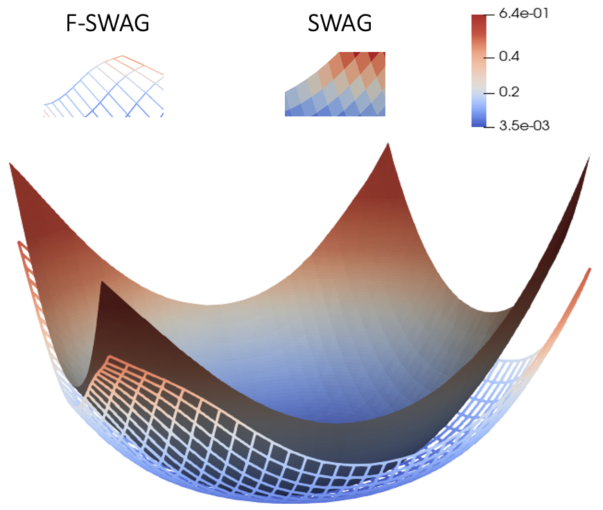
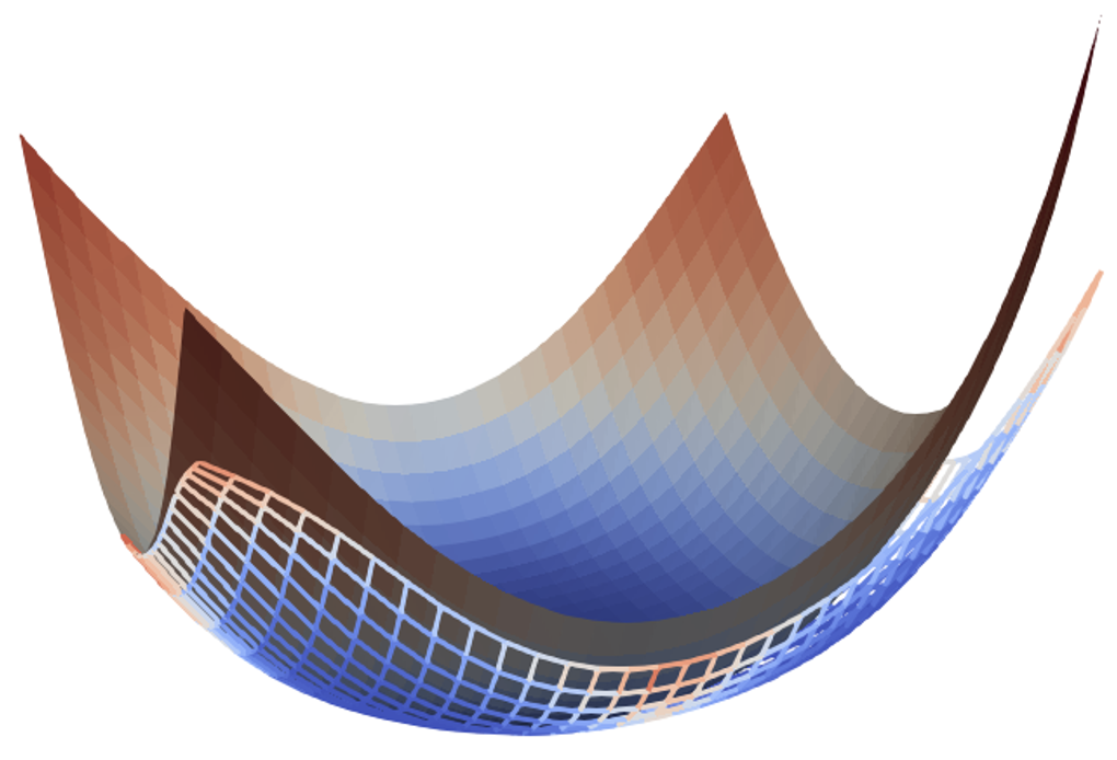
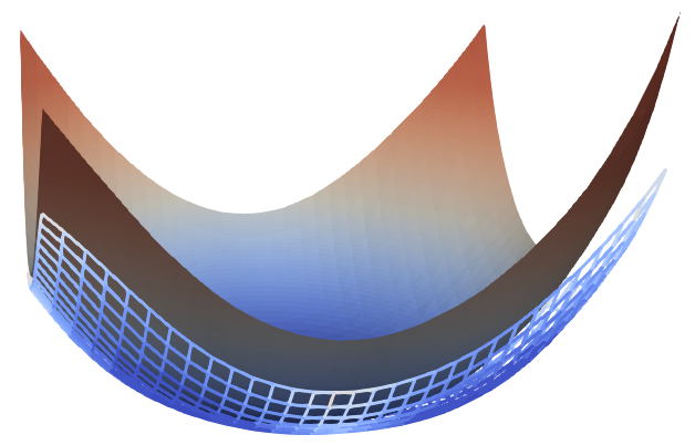
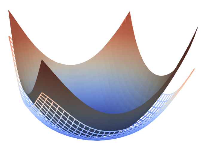
Figure 1: Comparing loss landscape of PreResNet-164 on CIFAR-100 dataset training with SWAG and F-SWAG method. For visualization purposes, we sample two models for each SWAG and F-SWAG and then plot the loss landscapes. It can be observed that the loss landscapes of our F-SWAG are flatter, supporting our argument for the flatter sampled models.

4.1 Experimental results

4.1.1 Predictive performance

Our experimental results, presented in Tables 1, 2, 3 for CIFAR-100 and CIFAR-10 dataset, and Table 4 for the ImageNet dataset, indicate a notable improvement across all experiments. It is worth noting that there is a trade-off between accuracy, negative log-likelihood, and expected calibration error. Nonetheless, our approach obtains a fine balance between these factors compared to the overall improvement.

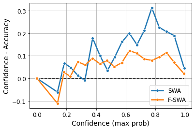
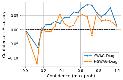
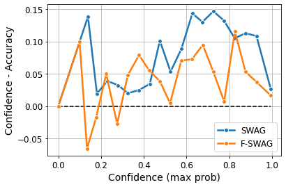
Figure 2: Reliability diagrams for PreResNet164 on CIFAR-100. The confidence is split into 20 bins and plots the gap between confidence and accuracy in each bin. The best case is the black dashed line when this gap is zeros. The plots of F-SWAG get closer to the zero lines, implying our F-SWAG can calibrate the uncertainty better.

4.2 Effectiveness of sharpness-aware posterior

Calibration of uncertainty estimates: We evaluate the ECE of each setting and compare it to baselines in Tables 1, 2, and 4. This score measures the maximum discrepancy between the accuracy and confidence of the model. To further clarify it, we display the Reliability Diagrams of PreResNet-164 on CIFAR-100 to understand how well the model predicts according to the confidence threshold in Figure 2. The experiments is detailed in the supplementary material.

Out-of-distribution prediction: The effectiveness of the sharpness-aware Bayesian neural network (BNN) is demonstrated in the above experiments, particularly in comparison to non-flat methods. In this section, we extend the evaluation to an out-of-distribution setting. Specifically, we utilize the BNN models trained on the CIFAR-10 dataset to assess their performance on the CIFAR-10-C dataset. This is an extension of the CIFAR-10 designed to evaluate the robustness of machine learning models against common corruptions and perturbations in the input data. The corruptions include various forms of noise, blur, weather conditions, and digital distortions. We conduct an ensemble of 30 models sampled from the flat-posterior distribution and compared them with non-flat ones. We present the average result of each corruption group and the average result on the whole dataset in Table 5, the detailed result of each corruption form is displayed in the supplementary material. Remarkably, the flat BNN models consistently surpass their non-flat counterparts with respect to average ECE and accuracy metrics. This finding is additional evidence of the generalization ability of the sharpness-aware posterior.

Table 5: Classification score on CIFAR-10-C on PreResNet-164 model when training with CIFAR-10. The full result on each type of corruption is displayed in the supplemetary material.

	ECE $\downarrow$				Accuracy $\uparrow$
Corruption	SWAG-D	F-SWAG-D	SWAG	F-SWAG	SWAG-D	F-SWAG-D	SWAG	F-SWAG
Noise	0.0729	0.0701	0.0958	0.0078	74.26	75.59	74.02	75.08
Blur	0.0121	0.0090	0.0202	0.0273	91.13	90.55	91.03	90.93
Weather	0.018	0.0142	0.0272	0.0240	89.47	89.18	89.42	89.11
Digital and others	0.0277	0.0229	0.0384	0.0209	87.03	86.94	86.93	87.19
Average	0.0328	0.0290	0.0454	0.0200	85.47	85.56	85.35	85.58

4.3 Ablation studies

In Figure 1, we plot the loss-landscape of the models sampled from our proposal of sharpness-aware posterior against the non-sharpness-aware one. Particularly, we compare two methods F-SWAG and SWAG by selecting four random models sampled from the posterior distribution of each method under the same hyper-parameter settings. As observed, our method not only improves the generalization of ensemble inference, demonstrated by classification results in Section 4.1 and sharpness in Section 4.2, but also the individual sampled model is flatter itself.

We measure and visualize the sharpness of the models. To this end, we sample five models from the approximate posteriors and then take the average of the sharpness of these models. For a model $\theta$, the sharpness is evaluated as $\displaystyle\max_{||\epsilon||_{2}\leq\rho}{\mathcal{L}_{\mathcal{S}}(\theta+\epsilon)-\mathcal{L}_{\mathcal{S}}(\theta)}$ to measure the change of loss value around $\theta$. We calculate the sharpness score of PreResNet-164 network for SWAG, and F-SWAG training on CIFAR-100 dataset and visualize them in the supplementary material. As shown there, the sharpness-aware versions produce smaller sharpness scores compared to the corresponding baselines, indicating that our models get into flatter regions.

5 Conclusion

In this paper, we introduce theories in the Bayesian setting and discuss variational inference for the sharpness-aware posterior in the context of Bayesian Neural Networks (BNNs). The sharpness-aware posterior results in models that are less sensitive to noise and have a better generalization ability, as it enables the models sampled from it and the optimal approximate posterior estimates to have a higher flatness. We conducted extensive experiments that leveraged the sharpness-aware posterior with state-of-the-art Bayesian Neural Networks. Our main results show that the models sampled from the proposed posterior outperform their baselines in terms of ensemble accuracy, expected calibration error (ECE), and negative log-likelihood (NLL). This indicates that the flat-seeking counterparts are better at capturing the true distribution of weights in neural networks and providing accurate probabilistic predictions. Furthermore, we performed ablation studies to showcase the effectiveness of the flat posterior distribution on various factors such as uncertainty estimation, loss landscape, and out-of-distribution prediction. Overall, the sharpness-aware posterior presents a promising approach for improving the generalization performance of Bayesian neural networks.

Acknowledgements.

This work was partly supported by ARC DP23 grant DP230101176 and by the Air Force Office of Scientific Research under award number FA2386-23-1-4044.

Appendix A Theoretical Development

A.1 All Proofs

Theorem A.1.

(Theorem 3.1 in the main paper) Consider the following optimization problem

$$\min_{\mathbb{Q<<\mathbb{P}}}\left\{\lambda\mathcal{L}_{S}\left(\mathbb{Q}\right)+KL\left(\mathbb{Q},\mathbb{P}\right)\right\},$$ (8)

where we search over $\mathbb{Q}$ absolutely continuous w.r.t. $\mathbb{P}$ and $KL\left(\cdot,\cdot\right)$ is the Kullback-Leibler divergence. This optimization has a closed-form optimal solution $\mathbb{Q}^{*}$ with the density

$$q^{*}\left(\theta\right)\propto\exp\left\{-\lambda\mathcal{L}_{\mathcal{S}}\left(\theta\right)\right\}p(\theta),$$

which is exactly the standard posterior $\mathbb{Q}_{\mathcal{S}}$ with the density $q(\theta\mid\mathcal{S})$.

Proof.

We have

$$\lambda\mathcal{L}_{S}\left(\mathbb{Q}\right)+KL\left(\mathbb{Q},\mathbb{P}\right)=\lambda\int\mathcal{L}_{S}\left(\theta\right)q\left(\theta\right)d\theta+\int q(\theta)\log\frac{q\left(\theta\right)}{p\left(\theta\right)}d\theta.$$

The Lagrange function is as follows

$$L\left(q,\alpha\right)=\lambda\int\mathcal{L}_{S}\left(\theta\right)q\left(\theta\right)d\theta+\int q(\theta)\log\frac{q\left(\theta\right)}{p\left(\theta\right)}d\theta+\alpha\left(\int q(\theta)d\theta-1\right).$$

Take derivative w.r.t. $q\left(\theta\right)$ and set it to $0$, we obtain

$$\lambda\mathcal{L}_{S}\left(\theta\right)+\log q\left(\theta\right)+1-\log p\left(\theta\right)+\alpha=0.$$

$$q\left(\theta\right)=\exp\left\{-\lambda\mathcal{L}_{S}\left(\theta\right)\right\}p\left(\theta\right)\exp\left\{-\alpha-1\right\}.$$

$$q\left(\theta\right)\propto\exp\left\{-\lambda\mathcal{L}_{S}\left(\theta\right)\right\}p\left(\theta\right).$$

∎

Lemma A.2.

Assume that the data space $\mathcal{X}$, the label space $\mathcal{Y}$, and the model space $\Theta$ are compact sets. There exist the modulus of continuity $\omega:\mathbb{R}^{+}\rightarrow\mathbb{R}^{+}$ with $\lim_{t\rightarrow 0^{+}}\omega\left(t\right)=0$ such that $\left|\ell\left(f_{\theta}\left(x\right),y\right)-\ell\left(f_{\theta^{\prime}}\left(x\right),y\right)\right|\leq\omega\left(\left\|\theta-\theta^{\prime}\right\|\right),\forall x\in\mathcal{X},y\in\mathcal{Y}$.

Proof.

The loss function $\ell\left(f_{\theta}\left(x\right),y\right)$ is continuous on the compact set $\mathcal{X}\times\mathcal{Y}\times\Theta$, hence it is equip-continuous on this set. For every $\epsilon>0$, there exists $\delta_{x},\delta_{y},\delta_{\theta}>0$ such that

$$\forall\left\|x^{\prime}-x\right\|\leq\delta_{x},\left\|y^{\prime}-y\right\|\leq\delta_{y},\left\|\theta^{\prime}-\theta\right\|\leq\delta_{\theta},$$

we have $\left|\ell\left(f_{\theta^{\prime}}\left(x^{\prime}\right),y^{\prime}\right)-\ell\left(f_{\theta^{\prime}}\left(x\right),y\right)\right|\leq\epsilon$.

Therefore, for all $\left\|\theta^{\prime}-\theta\right\|\leq\delta_{\theta}$, we have

$$\left|\ell\left(f_{\theta}\left(x\right),y\right)-\ell\left(f_{\theta^{\prime}}\left(x\right),y\right)\right|\leq\epsilon,\forall x,y.$$

This means that the family $\{\ell\left(f_{\theta}\left(x\right),y\right):x\in\mathcal{X},y\in\mathcal{Y}\}$ is equi-continuous w.r.t. $\theta\in\Theta$. This means the existence of the common modulus of continuity $\omega:\mathbb{R}^{+}\rightarrow\mathbb{R}^{+}$ with $\lim_{t\rightarrow 0^{+}}\omega\left(t\right)=0.$ ∎

Definition A.3.

Given $\epsilon>0$, we say that $\Theta$ is $\epsilon$-covered by a set $\Theta^{\prime}$ if for all $\theta\in\Theta$, there exists $\theta^{\prime}\in\Theta^{\prime}$ such that $\left\|\theta^{\prime}-\theta\right\|\leq\epsilon.$ We define $\mathcal{N}\left(\Theta,\epsilon\right)$ as the cardinality set of the smallest set $\Theta^{\prime}$ that covers $\Theta$.

Lemma A.4.

Let $R=\max_{\theta\in\Theta}\left\|\theta\right\|^{2}<\infty$ and $k$ is the dimension of $\Theta$. We can upper-bound the coverage number as

$$\mathcal{N}\left(\Theta,\epsilon\right)\leq\left(\frac{2R\sqrt{k}}{\epsilon}\right)^{k}.$$

Proof.

The proof can be found in Chapter 27 of [54]. ∎

By choosing $\epsilon=\frac{1}{n^{\frac{1}{2k}}}$, we obtain

$$\mathcal{N}\left(\Theta,n^{-\frac{1}{2k}}\right)\leq\left(2R\sqrt{k}\right)^{k}\sqrt{n}.$$

However, solving the optimization problem (OP) for the general data-label distribution $\mathcal{D}$ is generally intractable. To make it tractable, we find its upper-bound which is relevant to the sharpness as shown in the following theorem.

Theorem A.5.

(Theorem 3.2 in the main paper) Assume that $\Theta$ is a compact set. Given any $\delta\in[0;1]$, with the probability at least $1-\delta$ over the choice of $\mathcal{S}\sim\mathcal{D}^{n}$, for any distribution $\mathbb{Q}$, we have

$$\mathcal{L}_{\mathcal{D}}\left(\mathbb{Q}\right) \leq\mathbb{E}_{\theta\sim\mathbb{Q}}\left[\max_{\theta^{\prime}:\left\|\theta^{\prime}-\theta\right\|\leq\rho}\mathcal{L}_{\mathcal{S}}\left(\theta^{\prime}\right)\right]+\mathcal{L}_{\mathcal{S}}\left(\mathbb{Q}\right)+\frac{1}{\sqrt{n}}+2\omega\left(\frac{1}{n^{\frac{1}{2k}}}\right)$$

$$+\sqrt{\frac{k\left(1+\log\left(1+\frac{2R^{2}}{\rho^{2}}\left(1+2\log\left(2R\sqrt{k}\right)+\frac{2}{k}\log n\right)\right)\right)+2\log\frac{n}{\delta}}{4(n-1)}},$$

where we assume that $\mathcal{L}_{\mathcal{D}}\left(\mathbb{Q}\right)=\mathbb{E}_{\theta\sim\mathbb{Q}}\left[\mathcal{L}_{\mathcal{D}}\left(\theta\right)\right]\leq\mathbb{E}_{\theta\sim\mathbb{Q}}\left[\mathbb{E}_{\epsilon\sim\mathcal{N}(0,\sigma\mathbb{I})}\left[\mathcal{L}_{\mathcal{D}}\left(\theta+\epsilon\right)\right]\right]$ with $\sigma=\frac{\rho}{k^{1/2}\left(1+\sqrt{\frac{\log\left(N^{2}n\right)}{k}}\right)}$ and $N=\mathcal{N}\left(\Theta,n^{-\frac{1}{2k}}\right)$, $k$ is the number of parameters of the models, $n=\left|S\right|$, $R=\max_{\theta\in\Theta}\left\|\theta\right\|$, and $\omega:\mathbb{R}^{+}\rightarrow\mathbb{R}^{+}$ is a function such that $\lim_{t\rightarrow 0^{+}}\omega\left(t\right)=0$.

Proof.

Given $\epsilon=\frac{1}{n^{\frac{1}{2k}}}$, we denote $\Theta^{\prime}=\left\{\theta_{1}^{{}^{\prime}},\dots,\theta_{N}^{{}^{\prime}}\right\}$ where $N=\mathcal{N}\left(\Theta,n^{-\frac{1}{2k}}\right)\leq\left(2R\sqrt{k}\right)^{k}\sqrt{n}$ as the $\epsilon$-covered set of $\Theta$. We first examine a discrete distribution

$$\mathbb{Q}=\sum_{i=1}^{m}\pi_{i}\delta_{\theta_{i}}.$$

Without lossing the generalization, we can assume that $\left\|\theta_{i}^{{}^{\prime}}-\theta_{i}\right\|\leq\epsilon,\forall i=1,\dots,m$. We note that $\theta_{1}^{{}^{\prime}},\dots.\theta_{m}^{{}^{\prime}}$ can be repeated if $m>N$. Using Lemma A.2, let $\omega(\cdot)$ be the modulus of continuity of $\ell\left(f_{\theta}\left(x\right),y\right)$ such that $\left|\ell\left(f_{\theta}\left(x\right),y\right)-\ell\left(f_{\theta}\left(x\right),y\right)\right|\leq\omega\left(\left\|\theta-\theta^{\prime}\right\|\right),\forall x,y$ and $\lim_{t\rightarrow 0}\omega\left(t\right)=0$. This implies that

$$\left|\ell\left(f_{\theta_{i}}\left(x\right),y\right)-\ell\left(f_{\theta_{i}^{{}^{\prime}}}\left(x\right),y\right)\right|\leq\omega\left(\epsilon\right)=\omega\left(\frac{1}{n^{\frac{1}{2k}}}\right),\forall x,y,i=1,\dots,m.$$

We consider the distribution $\bar{\mathbb{Q}}=\sum_{i=1}^{m}\pi_{i}\mathcal{N}\left(\theta_{i}^{{}^{\prime}},\sigma\mathbb{I}\right)$. According to the McAllester PAC-Bayes bound, with the probability $1-\delta$ over the choices of $\mathcal{S}\sim\mathcal{D}^{n}$, for any distribution $\bar{\mathbb{P}}$, we have

$$\mathcal{L}_{\mathcal{D}}\left(\bar{\mathbb{Q}}\right)\leq\mathcal{L}_{S}\left(\bar{\mathbb{Q}}\right)+\sqrt{\frac{KL\left(\bar{\mathbb{Q}},\bar{\mathbb{P}}\right)+\log\frac{n}{\delta}}{2(n-1)}.}$$

Let $\theta^{*}=\underset{{}_{1\leq i\leq m}}{\text{argmax}}\left\|\theta_{i}^{{}^{\prime}}\right\|$. We consider the distribution $\bar{\mathbb{P}}=\mathcal{N}\left(0,\sigma_{\mathbb{P}}\right)$where $\sigma_{\mathbb{P}}^{2}=c\exp\left\{\frac{1-j}{k}\right\}$ with $c=\sigma^{2}\left(1+\exp\left\{\frac{4n}{k}\right\}\right)$ and $j=\left\lfloor 1+k\log\frac{c}{\sigma^{2}+\frac{\left\|\theta^{*}\right\|^{2}}{k}}\right\rfloor=\left\lfloor 1+k\log\frac{\sigma^{2}\left(1+\exp\left\{\frac{4n}{k}\right\}\right)}{\sigma^{2}+\frac{\left\|\theta^{*}\right\|^{2}}{k}}\right\rfloor$. It follows that

$$\sigma^{2}+\frac{\left\|\theta^{*}\right\|^{2}}{k}\leq\sigma_{\mathbb{P}}\leq\exp\left\{\frac{1}{k}\right\}\left(\sigma^{2}+\frac{\left\|\theta^{*}\right\|^{2}}{k}\right).$$

We have

$$KL\left(\mathcal{N}\left(\theta_{i}^{{}^{\prime}},\sigma\mathbb{I}\right),\bar{\mathbb{P}}\right)=\frac{1}{2}\left[\frac{k\sigma^{2}+\left\|\theta_{i}^{{}^{\prime}}\right\|^{2}}{\sigma_{\mathbb{P}}^{2}}-k+k\log\left(\frac{\sigma_{\mathbb{P}}^{2}}{\sigma^{2}}\right)\right].$$

$$KL\left(\mathcal{N}\left(\theta^{*},\sigma\mathbb{I}\right),\bar{\mathbb{P}}\right)=\max_{i}KL\left(\mathcal{N}\left(\theta_{i}^{{}^{\prime}},\sigma\mathbb{I}\right),\bar{\mathbb{P}}\right).$$

$$KL\left(\bar{\mathbb{Q}},\bar{\mathbb{P}}\right)\leq\sum_{i=1}^{m}\pi_{i}KL\left(\mathcal{N}\left(\theta_{i}^{{}^{\prime}},\sigma\mathbb{I}\right),\bar{\mathbb{P}}\right)\leq KL\left(\mathcal{N}\left(\theta^{*},\sigma\mathbb{I}\right),\bar{\mathbb{P}}\right).$$

We now bound $KL\left(\mathcal{N}\left(\theta^{*},\sigma\mathbb{I}\right),\bar{\mathbb{P}}\right)$

$$KL\left(\mathcal{N}\left(\theta^{*},\sigma\mathbb{I}\right),\bar{\mathbb{P}}\right) =\frac{1}{2}\left[\frac{k\sigma^{2}+\left\|\theta^{*}\right\|^{2}}{\sigma_{\mathbb{P}}^{2}}-k+k\log\left(\frac{\sigma_{\mathbb{P}}^{2}}{\sigma^{2}}\right)\right]$$

$$\leq \frac{1}{2}\left[\frac{k\sigma^{2}+\left\|\theta^{*}\right\|^{2}}{\sigma^{2}+\frac{\left\|\theta^{*}\right\|^{2}}{k}}-k+k\log\left(\frac{\exp\left\{\frac{1}{k}\right\}\left(\sigma^{2}+\frac{\left\|\theta^{*}\right\|^{2}}{k}\right)}{\sigma^{2}}\right)\right]$$

$$\leq \frac{k}{2}\left(1+\log\left(1+\frac{\left\|\theta^{*}\right\|^{2}}{k\sigma^{2}}\right)\right).$$

Therefore, with the probability $1-\delta$, we reach

$$\mathcal{L}_{\mathcal{D}}\left(\bar{\mathbb{Q}}\right)\leq\mathcal{L}_{S}\left(\bar{\mathbb{Q}}\right)+\sqrt{\frac{k\left(1+\log\left(1+\frac{\left\|\theta^{*}\right\|^{2}}{k\sigma^{2}}\right)\right)+2\log\frac{n}{\delta}}{4(n-1)}.}$$

$$\mathbb{E}_{\theta\sim\sum_{i=1}^{m}\pi_{i}\mathcal{N}\left(\theta_{i}^{{}^{\prime}},\sigma\mathbb{I}\right)}\left[\mathcal{L}_{\mathcal{D}}\left(\theta\right)\right] \leq\mathbb{E}_{\theta\sim\sum_{i=1}^{m}\pi_{i}\mathcal{N}\left(\theta_{i}^{{}^{\prime}},\sigma\mathbb{I}\right)}\left[\mathcal{L}_{\mathcal{S}}\left(\theta\right)\right]+\sqrt{\frac{k\left(1+\log\left(1+\frac{\left\|\theta^{*}\right\|^{2}}{k\sigma^{2}}\right)\right)+2\log\frac{n}{\delta}}{4(n-1)}.}$$

$$\leq \sum_{i=1}^{m}\pi_{i}\mathbb{E}_{\epsilon_{i}\sim\mathcal{N}\left(0,\sigma\mathbb{I}\right)}\left[\mathcal{L}_{\mathcal{S}}\left(\theta_{i}^{{}^{\prime}}+\epsilon_{i}\right)\right]+\sqrt{\frac{k\left(1+\log\left(1+\frac{\left\|\theta^{*}\right\|^{2}}{k\sigma^{2}}\right)\right)+2\log\frac{n}{\delta}}{4(n-1)}.}$$

Note that

$$\mathbb{E}_{\theta\sim\mathcal{N}\left(\theta_{i},\sigma\mathbb{I}\right)}\left[\mathcal{L}_{\mathcal{D}}\left(\theta\right)\right]-\mathbb{E}_{\theta\sim\mathcal{N}\left(\theta_{i}^{{}^{\prime}},\sigma\mathbb{I}\right)}\left[\mathcal{L}_{\mathcal{D}}\left(\theta\right)\right] =\int\left[\mathcal{L}_{\mathcal{D}}\left(\theta_{i}+\epsilon_{i}\right)-\mathcal{L}_{\mathcal{D}}\left(\theta_{i}^{{}^{\prime}}+\epsilon_{i}\right)\right]\mathcal{N}\left(\epsilon_{i}\mid 0,\sigma I\right)d\epsilon_{i}$$

$$\leq \int\omega\left(\frac{1}{n^{\frac{1}{2k}}}\right)\mathcal{N}\left(\epsilon_{i}\mid 0,\sigma I\right)d\epsilon_{i}=\omega\left(\frac{1}{n^{\frac{1}{2k}}}\right).$$

$$\mathbb{E}_{\theta\sim\mathcal{N}\left(\theta_{i},\sigma\mathbb{I}\right)}\left[\mathcal{L}_{\mathcal{D}}\left(\theta\right)\right]\leq\mathbb{E}_{\theta\sim\mathcal{N}\left(\theta_{i}^{{}^{\prime}},\sigma\mathbb{I}\right)}\left[\mathcal{L}_{\mathcal{D}}\left(\theta\right)\right]+\omega\left(\frac{1}{n^{\frac{1}{2k}}}\right).$$

$$\sum_{i=1}^{m}\pi_{i}\mathbb{E}_{\theta\sim\mathcal{N}\left(\theta_{i},\sigma\mathbb{I}\right)}\left[\mathcal{L}_{\mathcal{D}}\left(\theta\right)\right]\leq\sum_{i=1}^{m}\pi_{i}\mathbb{E}_{\theta\sim\mathcal{N}\left(\theta_{i}^{{}^{\prime}},\sigma\mathbb{I}\right)}\left[\mathcal{L}_{\mathcal{D}}\left(\theta\right)\right]+\omega\left(\frac{1}{n^{\frac{1}{2k}}}\right),$$

therefore we have

$$\mathbb{E}_{\theta\sim\sum_{i=1}^{m}\pi_{i}\mathcal{N}\left(\theta_{i},\sigma\mathbb{I}\right)}\left[\mathcal{L}_{\mathcal{D}}\left(\theta\right)\right] \leq\sum_{i=1}^{m}\pi_{i}\mathbb{E}_{\epsilon_{i}\sim\mathcal{N}\left(0,\sigma\mathbb{I}\right)}\left[\mathcal{L}_{\mathcal{S}}\left(\theta_{i}^{{}^{\prime}}+\epsilon_{i}\right)\right]$$

$$+\sqrt{\frac{k\left(1+\log\left(1+\frac{\left\|\theta^{*}\right\|^{2}}{k\sigma^{2}}\right)\right)+2\log\frac{n}{\delta}}{4(n-1)}}+\omega\left(\frac{1}{n^{\frac{1}{2k}}}\right).$$

Using the assumption

$$\mathcal{L}_{\mathcal{D}}\left(\mathbb{Q}\right)=\mathbb{E}_{\theta\sim\mathbb{Q}}\left[\mathcal{L}_{\mathcal{D}}\left(\theta\right)\right]\leq\mathbb{E}_{\theta\sim\mathbb{Q}}\left[\mathbb{E}_{\epsilon\sim\mathcal{N}\left(0,\sigma\mathbb{I}\right)}\left[\mathcal{L}_{\mathcal{D}}\left(\theta+\epsilon\right)\right]\right]=\mathbb{E}_{\theta\sim\sum_{i=1}^{m}\pi_{i}\mathcal{N}\left(\theta_{i},\sigma\mathbb{I}\right)}\left[\mathcal{L}_{\mathcal{D}}\left(\theta\right)\right],$$

we obtain

$$\mathcal{L}_{\mathcal{D}}\left(\mathbb{Q}\right) \leq\sum_{i=1}^{m}\pi_{i}\mathbb{E}_{\epsilon_{i}\sim\mathcal{N}\left(0,\sigma\mathbb{I}\right)}\left[\mathcal{L}_{\mathcal{S}}\left(\theta_{i}+\epsilon_{i}\right)\right]$$

$$+\sqrt{\frac{k\left(1+\log\left(1+\frac{R^{2}}{k\sigma^{2}}\right)\right)+2\log\frac{n}{\delta}}{4(n-1)}}+\omega\left(\frac{1}{n^{\frac{1}{2k}}}\right).$$

Because $\epsilon_{i}\sim\mathcal{N}\left(0,\sigma\mathbb{I}\right)$, $\left\|\epsilon_{i}\right\|^{2}$ follows the Chi-squared distribution. Therefore, we have for any $i\in[m]$

$$\mathbb{P}\left(\left\|\epsilon_{i}\right\|^{2}-k\sigma^{2}\geq 2\sigma^{2}\sqrt{kt}+2t\sigma^{2}\right)\leq\exp(-t),\forall t.$$

$$\mathbb{P}\left(\max_{i\in[m]}\left\|\epsilon_{i}\right\|^{2}-k\sigma^{2}\geq 2\sigma^{2}\sqrt{kt}+2t\sigma^{2}\right)\leq N\exp(-t),\forall t.,$$

since the cardinality of $\left|\{\theta_{1}^{{}^{\prime}},\dots.,\theta_{m}^{{}^{\prime}}\}\right|$ cannot exceed $N$.

$$\mathbb{P}\left(\max_{i\in[m]}\left\|\epsilon_{i}\right\|^{2}-k\sigma^{2}<2\sigma^{2}\sqrt{kt}+2t\sigma^{2}\right)>1-N\exp(-t),\forall t.$$

By choosing $t=\log\left(Nn^{1/2}\right),$ with the probability at least $1-\frac{1}{\sqrt{n}}$, we have for all $i\in[m]$

$$\left\|\epsilon_{i}\right\|^{2}<\sigma^{2}k\left(1+\frac{\log\left(N^{2}n\right)}{k}+2\sqrt{\frac{\log\left(Nn^{1/2}\right)}{k}}\right)\leq\sigma^{2}k\left(1+\sqrt{\frac{\log\left(N^{2}n\right)}{k}}\right)^{2}.$$

By choosing $\sigma=\frac{\rho}{k^{1/2}\left(1+\sqrt{\frac{\log\left(N^{2}n\right)}{k}}\right)}$, with the probability at least $1-\frac{1}{\sqrt{n}}$, we have for all $i\in[m]$

$$\left\|\epsilon_{i}\right\|<\rho.$$

We now derive

$$\mathcal{L}_{\mathcal{D}}\left(\mathbb{Q}\right) \leq\sum_{i=1}^{m}\pi_{i}\left(1-\frac{1}{\sqrt{n}}\right)\max_{\left\|\epsilon_{i}\right\|\leq\rho}\mathcal{L}_{\mathcal{S}}\left(\theta_{i}^{{}^{\prime}}+\epsilon_{i}\right)$$

$$+\frac{1}{\sqrt{n}}+\sqrt{\frac{k\left(1+\log\left(1+\frac{R^{2}}{k\sigma^{2}}\right)\right)+2\log\frac{n}{\delta}}{4(n-1)}}+\omega\left(\frac{1}{n^{\frac{1}{2k}}}\right)$$

$$\leq\left(1-\frac{1}{\sqrt{n}}\right)\sum_{i=1}^{m}\pi_{i}\max_{\left\|\epsilon_{i}\right\|\leq\rho}\mathcal{L}_{\mathcal{S}}\left(\theta_{i}^{{}^{\prime}}+\epsilon_{i}\right)+\frac{1}{\sqrt{n}}$$

$$+\sqrt{\frac{k\left(1+\log\left(1+\frac{R^{2}}{\rho^{2}}\left(1+\sqrt{\frac{\log\left(N^{2}n\right)}{k}}\right)^{2}\right)\right)+2\log\frac{n}{\delta}}{4(n-1)}}+\omega\left(\frac{1}{n^{\frac{1}{2k}}}\right)$$

$$\leq\sum_{i=1}^{m}\pi_{i}\max_{\left\|\epsilon_{i}\right\|\leq\rho}\mathcal{L}_{\mathcal{S}}\left(\theta_{i}^{{}^{\prime}}+\epsilon_{i}\right)+\frac{1}{\sqrt{n}}$$

$$+\sqrt{\frac{k\left(1+\log\left(1+\frac{2R^{2}}{\rho^{2}}\left(1+\frac{\log\left(N^{2}n\right)}{k}\right)\right)\right)+2\log\frac{n}{\delta}}{4(n-1)}}+\omega\left(\frac{1}{n^{\frac{1}{2k}}}\right)$$

$$\leq\sum_{i=1}^{m}\pi_{i}\max_{\left\|\epsilon_{i}\right\|\leq\rho}\mathcal{L}_{\mathcal{S}}\left(\theta_{i}^{{}^{\prime}}+\epsilon_{i}\right)+\frac{1}{\sqrt{n}}$$

$$+\sqrt{\frac{k\left(1+\log\left(1+\frac{2R^{2}}{\rho^{2}}\left(1+2\log\left(2R\sqrt{k}\right)+\frac{2}{k}\log n\right)\right)\right)+2\log\frac{n}{\delta}}{4(n-1)}}+\omega\left(\frac{1}{n^{\frac{1}{2k}}}\right).$$

Note that for all $i\in[m]$

$$\max_{\left\|\epsilon_{i}\right\|\leq\rho}\mathcal{L}_{\mathcal{S}}\left(\theta_{i}^{{}^{\prime}}+\epsilon_{i}\right)\leq\max_{\left\|\epsilon_{i}\right\|\leq\rho}\mathcal{L}_{\mathcal{S}}\left(\theta_{i}+\epsilon_{i}\right)+\omega\left(\frac{1}{n^{\frac{1}{2k}}}\right),$$

therefore, we reach

$$\mathcal{L}_{\mathcal{D}}\left(\mathbb{Q}\right) \leq\sum_{i=1}^{m}\pi_{i}\max_{\left\|\epsilon_{i}\right\|\leq\rho}\mathcal{L}_{\mathcal{S}}\left(\theta_{i}+\epsilon_{i}\right)+\frac{1}{\sqrt{n}}$$

$$+\sqrt{\frac{k\left(1+\log\left(1+\frac{2R^{2}}{\rho^{2}}\left(1+2\log\left(2R\sqrt{k}\right)+\frac{2}{k}\log n\right)\right)\right)+2\log\frac{n}{\delta}}{4(n-1)}}+2\omega\left(\frac{1}{n^{\frac{1}{2k}}}\right)$$

$$\leq\mathcal{L}_{\mathcal{S}}\left(\mathbb{Q}\right)+\frac{1}{\sqrt{n}}+2\omega\left(\frac{1}{n^{\frac{1}{2k}}}\right)$$

$$+\sqrt{\frac{k\left(1+\log\left(1+\frac{2R^{2}}{\rho^{2}}\left(1+2\log\left(2R\sqrt{k}\right)+\frac{2}{k}\log n\right)\right)\right)+2\log\frac{n}{\delta}}{4(n-1)}}.$$

For any distribution $\mathbb{Q}$, we approximate $\mathbb{Q}$ by its empirical distribution

$$\mathbb{Q}_{m}=\frac{1}{m}\sum_{i=1}^{m}\delta_{\theta_{i}},$$

which weakly converges to $\mathbb{Q}$ when $m\rightarrow\infty$. By using the achieved results for $\mathbb{Q}_{m}$ and taking limitation when $m\rightarrow\infty$, we reach the conclusion. ∎

Theorem A.6.

(Theorem 3.3 in the main paper) The optimal solution the OP in is the sharpness-aware posterior distribution $\mathbb{Q}_{S}^{SA}$ with the density function $q^{SA}(\theta|\mathcal{S})$:

$$q^{SA}(\theta|\mathcal{S}) \propto\exp\left\{-\lambda\max_{\theta^{\prime}:\left\|\theta^{\prime}-\theta\right\|\leq\rho}\mathcal{L}_{\mathcal{S}}\left(\theta^{\prime}\right)\right\}p\left(\theta\right)$$

$$=\exp\left\{-\lambda\mathcal{L}_{\mathcal{S}}\left(s\left(\theta\right)\right)\right\}p\left(\theta\right),$$

where we have defined $s\left(\theta\right)=\underset{{}_{\theta^{\prime}:\left\|\theta^{\prime}-\theta\right\|\leq\rho}}{\text{argmax}}\mathcal{L}_{\mathcal{S}}\left(\theta^{\prime}\right)$.

Proof.

We have

$$\lambda\mathbb{E}_{\theta\sim\mathbb{Q}}\left[\max_{\theta^{\prime}:\left\|\theta^{\prime}-\theta\right\|\leq\rho}\mathcal{L}_{\mathcal{S}}\left(\theta^{\prime}\right)\right]+KL\left(\mathbb{Q},\mathbb{P}\right)=\lambda\int\mathcal{L}_{S}\left(s\left(\theta\right)\right)q\left(\theta\right)d\theta+\int q(\theta)\log\frac{q\left(\theta\right)}{p\left(\theta\right)}d\theta.$$

The Lagrange function is as follows

$$L\left(q,\alpha\right)=\lambda\int\mathcal{L}_{S}\left(s(\theta)\right)q\left(\theta\right)d\theta+\int q(\theta)\log\frac{q\left(\theta\right)}{p\left(\theta\right)}d\theta+\alpha\left(\int q(\theta)d\theta-1\right).$$

Take derivative w.r.t. $q\left(\theta\right)$ and set it to $0$, we obtain

$$\lambda\mathcal{L}_{S}\left(s(\theta)\right)+\log q\left(\theta\right)+1-\log p\left(\theta\right)+\alpha=0.$$

$$q\left(\theta\right)=\exp\left\{-\lambda\mathcal{L}_{S}\left(s(\theta)\right)\right\}p\left(\theta\right)\exp\left\{-\alpha-1\right\}.$$

$$q\left(\theta\right)\propto\exp\left\{-\lambda\mathcal{L}_{S}\left(s(\theta)\right)\right\}p\left(\theta\right).$$

∎

A.2 Technicalities of the baselines and the corresponding flat versions

In what follows, we present how the baselines used in the experiments can be viewed as variational and MCMC approaches and incorporate our sharpness-aware technique.

Bayesian deep ensemble [35]:

We consider the approximate posterior $q_{\phi}=\frac{1}{K}\sum_{k=1}^{K}\delta_{\theta_{k}}$ where $\delta$ is the Dirac delta distribution as a uniform distribution over several base models $\theta_{1:K}$. Considering the prior distribution $p(\theta)=\mathcal{N}(0,\mathbb{I})$, we have the following OPs for the non-flat and flat versions.

Non-flat version:

$$\min_{\theta_{1:K}}\left\{\mathbb{E}_{\theta_{k}\sim q_{\phi}}\left[\lambda\mathcal{L}_{S}\left(\theta_{k}\right)\right]+KL\left(\frac{1}{K}\sum_{k=1}^{K}\delta_{\theta_{k}},\mathcal{N}\left(0,\mathbb{I}\right)\right)\right\},$$

where $KL\left(\frac{1}{K}\sum_{k=1}^{K}\delta_{\theta_{k}},\mathcal{N}\left(0,\mathbb{I}\right)\right)=-\frac{1}{K}\sum_{k=1}^{K}\log\mathcal{N}\left(\theta_{k}\mid 0,\mathbb{I}\right)+\text{const}$, leading to the L2 regularization terms.

Flat version:

$$\min_{\theta_{1:K}}\left\{\mathbb{E}_{\theta_{k}\sim q_{\phi}}\left[\lambda\max_{\theta^{\prime}:\|\theta^{\prime}-\theta_{k}\|\leq\rho}\mathcal{L}_{S}\left(\theta^{\prime}\right)\right]+KL\left(\frac{1}{K}\sum_{k=1}^{K}\delta_{\theta_{k}},\mathcal{N}\left(0,\mathbb{I}\right)\right)\right\}.$$

MC-Dropout [18]:

As shown in [18], the MC-dropout can be viewed as a BNN with the approximate posterior $q_{\phi}=\delta_{\phi}$ where $\phi$ is a fully-connected base model without any dropout and the prior distribution $p(\theta)=\mathcal{N}(0,\mathbb{I})$. The $KL(q_{\phi},p(\theta))$ can be approximated which turns out to be a weighted L2 regularization where the weights are proportional to the keep-prob rates at the layers. The main term $\mathbb{E}_{\theta\sim q_{\phi}}\left[\lambda\mathcal{L}_{S}\left(\theta\right)\right]$ can be interpreted as applying the dropout before minimizing the loss. For our flat version, the main term is $\mathbb{E}_{\theta\sim q_{\phi}}\left[\lambda\max_{\theta^{\prime}:\|\theta^{\prime}-\theta\|\leq\rho}\mathcal{L}_{S}\left(\theta^{\prime}\right)\right]$.

BNNs with Stochastic Gradient Langevin Dynamics (SGLD) [59]:

For SGLD, we sample one or several particle models directly from the posterior distribution $q(\theta\mid S)$ for the non-flat version and from the SA-posterior distribution $q^{SA}(\theta\mid S)$ for the flat version. For the non-flat version, the update is similar to the mini-batch SGD except that we add small Gaussian noises to the particle models. For our flat version, we first compute the perturbed model $\theta^{a}$ for a given particle model $\theta$ and use the mini-batch SGD update with the gradient evaluated at $\theta^{a}$ together with small Gaussian noises.

SWAG [39]:

We consider SWAG as an MCMC approach, where we keep a trajectory of particle models using SWA. Additionally, the covariance matrices are determined based on this trajectory to form an approximate Gaussian posterior. In the corresponding flat version to this approach, we employ SWA to sample from the SA (Sharpness-Aware) posterior. Specifically, we first calculate the perturbed model $\theta^{a}$ based on the current model $\theta$ and then employ mini-batch SGD updates with the gradient evaluated at model $\theta^{a}$. Finally, we update the final model using the SWA strategy.

Appendix B Additional experiments

B.1 Comparison with bSAM method

We conduct experiments to compare our flat BNN with bSAM [40] on Resnet18, the results are shown in Table 6. The authors of bSAM explored the relationship between SAM and BNN and proposed a combination of SAM and Adam to optimize the mean of parameters in BNN networks while keeping the variance fixed. The results clearly indicate that our flat BNN outperforms bSAM in most metric scores. Here we note that we are unable to evaluate bSAM on the architectures used in Tables 1 and 2 in the main paper because the authors did not release the code. Instead, we run our methods with the setting mentioned in the bSAM paper.

Table 6: Classification score on Resnet18

	CIFAR-10			CIFAR-100
Method	ACC $\uparrow$	NLL $\downarrow$	ECE $\downarrow$	ACC $\uparrow$	NLL $\downarrow$	ECE $\downarrow$
bSAM	96.15	0.1200	0.0049	80.22	0.7000	0.0310
F-SWAG-Diag	96.56	0.1047	0.0037	80.70	0.7012	0.0227
F-SWAG	96.58	0.1045	0.0045	80.74	0.7024	0.0243

Table 7: Classification score on CIFAR-10-C using PreResNet-164 model when training with CIFAR-10 dataset

	ECE $\downarrow$				Accuracy $\uparrow$
Method	SWAG-D	F-SWAG-D	SWAG	F-SWAG		SWAG-D	F-SWAG-D	SWAG	F-SWAG
Gaussian noise	0.0765	0.0765	0.1032	0.0091		72.01	73.95	71.58	73.43
Shot noise	0.0661	0.0647	0.0892	0.0075		75.77	77.09	75.44	76.28
Speckle noise	0.0711	0.0686	0.0921	0.0072		75.55	76.71	75.36	76.15
Impulse noise	0.0779	0.0706	0.0988	0.0077		73.74	74.61	73.71	74.49
Defocus blur	0.0108	0.0071	0.0178	0.0256		92.16	91.55	92.14	91.63
Gaussian blur	0.0130	0.0116	0.0214	0.0239		90.79	89.73	90.67	90.22
Motion blur	0.0147	0.0103	0.0233	0.0298		90.33	90.22	90.20	90.52
Zoom blur	0.0099	0.0070	0.0185	0.0301		91.24	90.71	91.12	91.36
snow	0.0298	0.0245	0.0419	0.0208		86.17	86.11	86.10	85.81
Fog	0.0114	0.0075	0.0176	0.0259		91.67	91.22	91.64	91.27
Brightness	0.0081	0.0076	0.0129	0.0281		93.47	92.94	93.45	92.98
Contrast	0.0110	0.0127	0.0141	0.0306		91.34	90.59	91.36	90.73
Elastic transform	0.0244	0.0213	0.0367	0.0220		87.06	86.61	86.98	86.94
Pixelate	0.0350	0.0269	0.0463	0.0124		85.75	86.11	85.61	85.74
Jpeg compression	0.0605	0.0522	0.0813	0.0093		78.01	78.90	77.57	79.80
Spatter	0.0242	0.0163	0.0341	0.0227		87.94	87.61	87.99	88.13
Saturate	0.0112	0.0080	0.0179	0.0288		92.10	91.79	92.09	91.81
Frost	0.0253	0.0174	0.0365	0.0215		86.60	86.48	86.52	86.39
Average	0.0322	0.0283	0.0446	0.0201		85.65	85.71	85.52	85.76

B.2 Full result of Out-of-distribution prediction

In Section 4.2 of the main paper, we provide a comprehensive analysis of the performance concerning various corruption groups, including noise, blur, weather conditions, and digital distortions. We present the detailed results for each corruption type in Table 7, providing a deeper understanding of the impact of these corruptions on the model’s performance. On average, flat BNNs outperform their non-flat counterparts, especially on ECE with a notable margin. These findings further emphasize the effectiveness of flat BNNs in enhancing robustness and generalization against various corruptions.

B.3 Additional ablation studies

Comparison of Hessian eigenvalue We report the log scale of the largest eigenvalue of the Hessian matrix over several methods applying to WideResNet28x10 using CIFAR-100, and the ratio of the largest and fifth eigenvalue as shown in Table 8, which evidently indicates that our method updates models to minima having lower curvature.

Table 8: Log scale of Hessian eigenvalue of WideResNet28x10 training on CIFAR-100. $\lambda_{1}$ is the largest eigenvalue and $\lambda_{5}$ is 5th largest eigenvalue

Method	$\lambda_{1}$ $\downarrow$	$\lambda_{1}$/$\lambda_{5}$
SWAG	4.17 $\pm$ 0.001	1.17 $\pm$ 0.012
F-SWAG	4.08 $\pm$ 0.000	1.17 $\pm$ 0.020
SGLD	3.34 $\pm$ 0.031	1.17 $\pm$ 0.009
F-SGLD	2.83$\pm$ 0.029	1.15 $\pm$ 0.010
Deep-ensemble	4.64 $\pm$ 0.055	1.45 $\pm$ 0.020
F-Deep-ensemble	4.01 $\pm$ 0.054	1.58 $\pm$ 0.032

Computational cost Our flat-seeking method requires the computation of gradients twice: initially to obtain the perturbed model $\theta^{\prime}$ and subsequently to update the model. Consequently, the training time is nearly double in comparison to non-flat counterparts, as indicated in Table 9. Note that the Deep Ensemble settings utilize multiple models training individually for prediction and we report training time for one model in each setting.

Table 9: Comparison of training time per epoch

Network & Dataset	SWAG	F-SWAG	SGLD	F-SGLD	Deep-ensemble	F-Deep-ensemble
WideResNet28x10 & CIFAR-100	110s	169s	110s	233s	110s	218s
Densenet-161 & ImageNet	1.75h	2.28h	1.78h	2.49h	-	-
ResNet-152 & ImageNet	1.59h	2.15h	1.64h	2.22h	-	-

The effect of $KL$ term in Deep-ensemble settings We present the results of training Deep-ensemble with SAM following the formula for the flat version in Section A.2 but without KL (or L2 regularisation) in Table 10. Each experiment is performed three times and reports the mean and standard deviation. Based on the result, without KL loss, our method still manages to yield better numbers than the non-flat counterparts.

Table 10: Experiments of F-Deep-ensemble variations on CIFAR-100 dataset using WideResNet28x10. Each experiment is conducted with three different random seeds to calculate mean and standard deviation

	WideResNet28x10
Model	ACC $\uparrow$	NLL $\downarrow$	ECE $\downarrow$
Deep-ensemble	83.04 $\pm$ 0.15	0.6958 $\pm$ 0.0335	0.0483 $\pm$ 0.0017
F-Deep-ensemble (Our)	84.52 $\pm$ 0.03	0.5644 $\pm$ 0.0106	0.0191 $\pm$ 0.0039
F-Deep-ensemble (w/o L2)	83.80 $\pm$ 0.10	0.7026 $\pm$ 0.0007	0.0594 $\pm$ 0.0005

Appendix C Experimental settings

CIFAR: We conduct experiments using PreResNet-164, WideResNet28x10, Resnet10 and Resnet18 on both CIFAR-10 and CIFAR-100. The total number of images in these datasets is 60,000, which comprises 50,000 instances for training and 10,000 for testing. For each network-dataset pair, we apply Sharpness-Aware Bayesian methodology to various settings, including F-SGLD, F-SGVB, F-SWAG-Diag, F-SWAG, F-MC-Dropout, and F-Deep-Ensemble.

In the experiments presented in Tables 1 and 2 in the main paper, we train all models for 300 epochs using SGD, with a learning rate of 0.1 and a cosine schedule. We start collecting models after epoch 161 for the F-SWA and F-SWAG settings, consistent with the protocol in [39]. Additionally, we set $\rho=0.05$ for CIFAR-10 and $\rho=0.1$ for CIFAR-100 in all experiments, except for Resnet10 and Resnet18, where $\rho$ is set to 0.01. The training set is augmented with basic data augmentations, including horizontal flip, padding by four pixels, random crop, and normalization. For the experiments presented in Table 3 in the main paper, we apply the same augmentations to the training set as in the experiments in Tables 1 and 2. However, the models are trained for 200 epochs using the Adam optimizer, with a learning rate of 0.001 and a plateau schedule. It’s worth noting that SGVB and SGVB-LRT perform poorly with other settings than those mentioned, making it challenging to scale up this approach.

For the baseline of the Deep-Ensemble, SGLD, SGVB and SGVB-LRT methods, we reproduce results following the hyper-parameters and processes as our flat versions. Note that we train three independent models for the Deep-Ensemble method. For inference, we do an ensemble on 30 sample models for all settings sampled from posterior distributions. To ensure the stability of the method, we repeat each set three times with different random seeds and report the mean and standard deviation.

ImageNet: This is a large and challenging dataset with 1000 classes. We conduct experiments with Densenet-161 and ResNet-152 architecture on F-SWAG-Diag, F-SWAG, and F-SGLD. For all settings, we initialize the models with pre-trained weights on the ImageNet dataset, obtained from the torchvision package, then fine-tuned for 10 epochs with $\rho=0.05$. We start collecting 4 models per epoch at the beginning of the fine-tuning process and evaluate them following a protocol consistent with the CIFAR dataset experiments.

The performance metrics for the SWAG-Diag, SWAG, and MC-Dropout methods are sourced from the original paper by Maddox et al. [39], except for the MC-Dropout result on PreResNet-164 for the CIFAR-100 dataset, which we reproduce due to its unavailability. The performance of bSAM is taken from [40].

It’s important to note that the purpose of these experiments was not to achieve state-of-the-art performance. Instead, we aim to demonstrate the utility of the sharpness-aware posterior when integrated with specific Bayesian Neural Networks. The implementation is provided in https://github.com/anh-ntv/flat_bnn.git.

Hyper-parameters for training: Table 11 provides our setup for both training and testing phases. Note that the SWAG-Diag method follows the same setup as SWAG. Typically, using the default $\rho=0.05$ yields a good performance across all experiments. However, $\rho=0.1$ is recommended for the CIFAR-100 dataset in [16]. For model evaluation, we use the checkpoint from the final epoch without taking into account the validation set’s performance.

Table 11: Hyperparameters for training both flat and non-flat versions of BNNs. All models are trained with the input resolution of $224\times 224$ and cosine learning rate decay, except experiments of SGVB and SGVB-LRT, which use an input resolution of $32\times 32$

Model	Method	Init weight	Epoch	LR init	Weight decay	$\rho$	# samples
CIFAR-100
PreResNet-164	SWAG						30
	MC-Drop	Scratch	300	0.1	3e-4	0.1	30
	Deep-Ens						3
WideResNet28x10	SWAG						30
	MC-Drop	Scratch	300	0.1	5e-4	0.1	30
	Deep-Ens						3
Resnet10	SGVB					5e-3
	F-SGVB + Geometry					5e-4
	SGVB-LRT	Scratch	200	0.001	5e-4	5e-3	30
	F-SGVB-LRT + Geometry					5e-4
Resnet18	SGVB					5e-3
	F-SGVB + Geometry					5e-4
	SGVB-LRT	Scratch	200	0.001	5e-4	5e-3	30
	F-SGVB-LRT + Geometry					5e-4
	SWAG	Scratch	300	0.1	5e-4	0.1	30
CIFAR-10
PreResNet-164	SWAG						30
	MC-Drop	Scratch	300	0.1	3e-4	0.05	30
	Deep-Ens						3
WideResNet28x10	SWAG						30
	MC-Drop	Scratch	300	0.1	5e-4	0.05	30
	Deep-Ens						3
Resnet10	SGVB					5e-3
	F-SGVB + Geometry					5e-4
	SGVB-LRT	Scratch	200	0.001	5e-4	5e-3	30
	F-SGVB-LRT + Geometry					5e-4
Resnet18	SGVB					5e-3
	F-SGVB + Geometry					5e-4
	SGVB-LRT	Scratch	200	0.001	5e-4	5e-3	30
	F-SGVB-LRT + Geometry					5e-4
	SWAG	Scratch	300	0.1	5e-4	0.1	30
ImageNet
DenseNet-161	All methods	Pre-trained	10	0.001	1e-4	0.05	30
ResNet-152	All methods	Pre-trained	10	0.001	1e-4	0.05	30

References

- [1] Momin Abbas, Quan Xiao, Lisha Chen, Pin-Yu Chen, and Tianyi Chen. Sharp-maml: Sharpness-aware model-agnostic meta learning. arXiv preprint arXiv:2206.03996, 2022.
- [2] Pierre Alquier, James Ridgway, and Nicolas Chopin. On the properties of variational approximations of gibbs posteriors. The Journal of Machine Learning Research, 17(1):8374–8414, 2016.
- [3] Dara Bahri, Hossein Mobahi, and Yi Tay. Sharpness-aware minimization improves language model generalization. In Proceedings of the 60th Annual Meeting of the Association for Computational Linguistics (Volume 1: Long Papers), pages 7360–7371, Dublin, Ireland, May 2022. Association for Computational Linguistics.
- [4] Jose Blanchet and Karthyek Murthy. Quantifying distributional model risk via optimal transport. Mathematics of Operations Research, 44(2):565–600, 2019.
- [5] Charles Blundell, Julien Cornebise, Koray Kavukcuoglu, and Daan Wierstra. Weight uncertainty in neural network. In International conference on machine learning, pages 1613–1622. PMLR, 2015.
- [6] Stephen Boyd and Lieven Vandenberghe. Convex Optimization. Cambridge University Press, March.
- [7] Olivier Catoni. Pac-bayesian supervised classification: the thermodynamics of statistical learning. arXiv preprint arXiv:0712.0248, 2007.
- [8] Junbum Cha, Sanghyuk Chun, Kyungjae Lee, Han-Cheol Cho, Seunghyun Park, Yunsung Lee, and Sungrae Park. Swad: Domain generalization by seeking flat minima. Advances in Neural Information Processing Systems, 34:22405–22418, 2021.
- [9] Pratik Chaudhari, Anna Choromańska, Stefano Soatto, Yann LeCun, Carlo Baldassi, Christian Borgs, Jennifer T. Chayes, Levent Sagun, and Riccardo Zecchina. Entropy-sgd: biasing gradient descent into wide valleys. Journal of Statistical Mechanics: Theory and Experiment, 2019, 2017.
- [10] Tianqi Chen, Emily Fox, and Carlos Guestrin. Stochastic gradient hamiltonian monte carlo. In International conference on machine learning, pages 1683–1691. PMLR, 2014.
- [11] Xiangning Chen, Cho-Jui Hsieh, and Boqing Gong. When vision transformers outperform resnets without pre-training or strong data augmentations. arXiv preprint arXiv:2106.01548, 2021.
- [12] Laurent Dinh, Razvan Pascanu, Samy Bengio, and Yoshua Bengio. Sharp minima can generalize for deep nets. In International Conference on Machine Learning, pages 1019–1028. PMLR, 2017.
- [13] Jiawei Du, Daquan Zhou, Jiashi Feng, Vincent YF Tan, and Joey Tianyi Zhou. Sharpness-aware training for free. arXiv preprint arXiv:2205.14083, 2022.
- [14] Michael Dusenberry, Ghassen Jerfel, Yeming Wen, Yian Ma, Jasper Snoek, Katherine Heller, Balaji Lakshminarayanan, and Dustin Tran. Efficient and scalable bayesian neural nets with rank-1 factors. In International conference on machine learning, pages 2782–2792. PMLR, 2020.
- [15] Gintare Karolina Dziugaite and Daniel M. Roy. Computing nonvacuous generalization bounds for deep (stochastic) neural networks with many more parameters than training data. In UAI. AUAI Press, 2017.
- [16] Pierre Foret, Ariel Kleiner, Hossein Mobahi, and Behnam Neyshabur. Sharpness-aware minimization for efficiently improving generalization. In International Conference on Learning Representations, 2021.
- [17] Stanislav Fort and Surya Ganguli. Emergent properties of the local geometry of neural loss landscapes. arXiv preprint arXiv:1910.05929, 2019.
- [18] Yarin Gal and Zoubin Ghahramani. Dropout as a bayesian approximation: Representing model uncertainty in deep learning. In Maria Florina Balcan and Kilian Q. Weinberger, editors, Proceedings of The 33rd International Conference on Machine Learning, volume 48 of Proceedings of Machine Learning Research, pages 1050–1059, New York, New York, USA, 20–22 Jun 2016. PMLR.
- [19] Yarin Gal, Jiri Hron, and Alex Kendall. Concrete dropout. Advances in neural information processing systems, 30, 2017.
- [20] Soumya Ghosh, Jiayu Yao, and Finale Doshi-Velez. Structured variational learning of bayesian neural networks with horseshoe priors. In International Conference on Machine Learning, pages 1744–1753. PMLR, 2018.
- [21] Alex Graves. Practical variational inference for neural networks. Advances in neural information processing systems, 24, 2011.
- [22] Arjun K Gupta and Daya K Nagar. Matrix variate distributions. Chapman and Hall/CRC, 2018.
- [23] Sepp Hochreiter and Jürgen Schmidhuber. Simplifying neural nets by discovering flat minima. In NIPS, pages 529–536. MIT Press, 1994.
- [24] Pavel Izmailov, Dmitrii Podoprikhin, Timur Garipov, Dmitry Vetrov, and Andrew Gordon Wilson. Averaging weights leads to wider optima and better generalization. arXiv preprint arXiv:1803.05407, 2018.
- [25] Pavel Izmailov, Dmitrii Podoprikhin, Timur Garipov, Dmitry P. Vetrov, and Andrew Gordon Wilson. Averaging weights leads to wider optima and better generalization. In UAI, pages 876–885. AUAI Press, 2018.
- [26] Stanislaw Jastrzebski, Zachary Kenton, Devansh Arpit, Nicolas Ballas, Asja Fischer, Yoshua Bengio, and Amos J. Storkey. Three factors influencing minima in sgd. ArXiv, abs/1711.04623, 2017.
- [27] Yiding Jiang, Behnam Neyshabur, Hossein Mobahi, Dilip Krishnan, and Samy Bengio. Fantastic generalization measures and where to find them. In ICLR. OpenReview.net, 2020.
- [28] Jean Kaddour, Linqing Liu, Ricardo Silva, and Matt Kusner. When do flat minima optimizers work? In Alice H. Oh, Alekh Agarwal, Danielle Belgrave, and Kyunghyun Cho, editors, Advances in Neural Information Processing Systems, 2022.
- [29] Nitish Shirish Keskar, Dheevatsa Mudigere, Jorge Nocedal, Mikhail Smelyanskiy, and Ping Tak Peter Tang. On large-batch training for deep learning: Generalization gap and sharp minima. In ICLR. OpenReview.net, 2017.
- [30] Mohammad Khan, Didrik Nielsen, Voot Tangkaratt, Wu Lin, Yarin Gal, and Akash Srivastava. Fast and scalable bayesian deep learning by weight-perturbation in adam. In International Conference on Machine Learning, pages 2611–2620. PMLR, 2018.
- [31] Minyoung Kim, Da Li, Shell X Hu, and Timothy Hospedales. Fisher SAM: Information geometry and sharpness aware minimisation. In Kamalika Chaudhuri, Stefanie Jegelka, Le Song, Csaba Szepesvari, Gang Niu, and Sivan Sabato, editors, Proceedings of the 39th International Conference on Machine Learning, volume 162 of Proceedings of Machine Learning Research, pages 11148–11161. PMLR, 17–23 Jul 2022.
- [32] Diederik P Kingma and Max Welling. Auto-encoding variational bayes. arXiv preprint arXiv:1312.6114, 2013.
- [33] Durk P Kingma, Tim Salimans, and Max Welling. Variational dropout and the local reparameterization trick. Advances in neural information processing systems, 28, 2015.
- [34] Jungmin Kwon, Jeongseop Kim, Hyunseo Park, and In Kwon Choi. Asam: Adaptive sharpness-aware minimization for scale-invariant learning of deep neural networks. In International Conference on Machine Learning, pages 5905–5914. PMLR, 2021.
- [35] Balaji Lakshminarayanan, Alexander Pritzel, and Charles Blundell. Simple and scalable predictive uncertainty estimation using deep ensembles. Advances in neural information processing systems, 30, 2017.
- [36] Qiang Liu and Dilin Wang. Stein variational gradient descent: A general purpose bayesian inference algorithm. Advances in neural information processing systems, 29, 2016.
- [37] Yong Liu, Siqi Mai, Xiangning Chen, Cho-Jui Hsieh, and Yang You. Towards efficient and scalable sharpness-aware minimization. In Proceedings of the IEEE/CVF Conference on Computer Vision and Pattern Recognition, pages 12360–12370, 2022.
- [38] Christos Louizos and Max Welling. Multiplicative normalizing flows for variational bayesian neural networks. In International Conference on Machine Learning, pages 2218–2227. PMLR, 2017.
- [39] Wesley J. Maddox, Timur Garipov, Pavel Izmailov, Dmitry Vetrov, and Andrew Gordon Wilson. A Simple Baseline for Bayesian Uncertainty in Deep Learning. Curran Associates Inc., Red Hook, NY, USA, 2019.
- [40] Thomas Möllenhoff and Mohammad Emtiyaz Khan. Sam as an optimal relaxation of bayes. arXiv preprint arXiv:2210.01620, 2022.
- [41] Radford M. Neal. Bayesian Learning for Neural Networks. Springer-Verlag, Berlin, Heidelberg, 1996.
- [42] Behnam Neyshabur, Srinadh Bhojanapalli, David McAllester, and Nati Srebro. Exploring generalization in deep learning. Advances in neural information processing systems, 30, 2017.
- [43] Son Nguyen, Duong Nguyen, Khai Nguyen, Khoat Than, Hung Bui, and Nhat Ho. Structured dropout variational inference for bayesian neural networks. Advances in Neural Information Processing Systems, 34:15188–15202, 2021.
- [44] Van-Anh Nguyen, Trung Le, Anh Bui, Thanh-Toan Do, and Dinh Phung. Optimal transport model distributional robustness. In Advances in Neural Information Processing Systems, 2023.
- [45] Victor M-H Ong, David J Nott, and Michael S Smith. Gaussian variational approximation with a factor covariance structure. Journal of Computational and Graphical Statistics, 27(3):465–478, 2018.
- [46] Gabriel Pereyra, George Tucker, Jan Chorowski, Lukasz Kaiser, and Geoffrey E. Hinton. Regularizing neural networks by penalizing confident output distributions. In ICLR (Workshop). OpenReview.net, 2017.
- [47] Henning Petzka, Michael Kamp, Linara Adilova, Cristian Sminchisescu, and Mario Boley. Relative flatness and generalization. In NeurIPS, pages 18420–18432, 2021.
- [48] Cuong Pham, C. Cuong Nguyen, Trung Le, Phung Dinh, Gustavo Carneiro, and Thanh-Toan Do. Model and feature diversity for bayesian neural networks in mutual learning. In Advances in Neural Information Processing Systems, 2023.
- [49] Hoang Phan, Trung Le, Trung Phung, Anh Tuan Bui, Nhat Ho, and Dinh Phung. Global-local regularization via distributional robustness. In Francisco Ruiz, Jennifer Dy, and Jan-Willem van de Meent, editors, Proceedings of The 26th International Conference on Artificial Intelligence and Statistics, volume 206 of Proceedings of Machine Learning Research, pages 7644–7664. PMLR, 25–27 Apr 2023.
- [50] Hoang Phan, Lam Tran, Ngoc N Tran, Nhat Ho, Dinh Phung, and Trung Le. Improving multi-task learning via seeking task-based flat regions. arXiv preprint arXiv:2211.13723, 2022.
- [51] Zhe Qu, Xingyu Li, Rui Duan, Yao Liu, Bo Tang, and Zhuo Lu. Generalized federated learning via sharpness aware minimization. arXiv preprint arXiv:2206.02618, 2022.
- [52] Hippolyt Ritter, Aleksandar Botev, and David Barber. A scalable laplace approximation for neural networks. In 6th International Conference on Learning Representations, ICLR 2018-Conference Track Proceedings, volume 6. International Conference on Representation Learning, 2018.
- [53] Simone Rossi, Sebastien Marmin, and Maurizio Filippone. Walsh-hadamard variational inference for bayesian deep learning. Advances in Neural Information Processing Systems, 33:9674–9686, 2020.
- [54] Shai Shalev-Shwartz and Shai Ben-David. Understanding machine learning: From theory to algorithms. Cambridge university press, 2014.
- [55] Jakub Swiatkowski, Kevin Roth, Bastiaan Veeling, Linh Tran, Joshua Dillon, Jasper Snoek, Stephan Mandt, Tim Salimans, Rodolphe Jenatton, and Sebastian Nowozin. The k-tied normal distribution: A compact parameterization of gaussian mean field posteriors in bayesian neural networks. In International Conference on Machine Learning, pages 9289–9299. PMLR, 2020.
- [56] Marcin Tomczak, Siddharth Swaroop, and Richard Turner. Efficient low rank gaussian variational inference for neural networks. Advances in Neural Information Processing Systems, 33:4610–4622, 2020.
- [57] Tuan Truong, Hoang-Phi Nguyen, Tung Pham, Minh-Tuan Tran, Mehrtash Harandi, Dinh Phung, and Trung Le. Rsam: Learning on manifolds with riemannian sharpness-aware minimization, 2023.
- [58] Colin Wei, Sham Kakade, and Tengyu Ma. The implicit and explicit regularization effects of dropout. In International conference on machine learning, pages 10181–10192. PMLR, 2020.
- [59] Max Welling and Yee W Teh. Bayesian learning via stochastic gradient langevin dynamics. In Proceedings of the 28th international conference on machine learning (ICML-11), pages 681–688, 2011.
- [60] Guodong Zhang, Shengyang Sun, David Duvenaud, and Roger Grosse. Noisy natural gradient as variational inference. In International Conference on Machine Learning, pages 5852–5861. PMLR, 2018.
- [61] Linfeng Zhang, Jiebo Song, Anni Gao, Jingwei Chen, Chenglong Bao, and Kaisheng Ma. Be your own teacher: Improve the performance of convolutional neural networks via self distillation. In Proceedings of the IEEE/CVF International Conference on Computer Vision, pages 3713–3722, 2019.
- [62] Ying Zhang, Tao Xiang, Timothy M. Hospedales, and Huchuan Lu. Deep mutual learning. 2018 IEEE/CVF Conference on Computer Vision and Pattern Recognition, pages 4320–4328, 2018.
- [63] Juntang Zhuang, Boqing Gong, Liangzhe Yuan, Yin Cui, Hartwig Adam, Nicha Dvornek, Sekhar Tatikonda, James Duncan, and Ting Liu. Surrogate gap minimization improves sharpness-aware training. arXiv preprint arXiv:2203.08065, 2022.