Glancing through the debris disk: Photometric analysis of DE Boo with CHEOPS

Abstract

Aims. DE Boo is a unique system, with an edge-on view through the debris disk around the star. The disk, which is analogous to the Kuiper belt in the Solar System, was reported to extend from 74 to 84 AU from the central star. The high photometric precision of the Characterising Exoplanet Satellite (CHEOPS) provided an exceptional opportunity to observe small variations in the light curve due to transiting material in the disk. This is a unique chance to investigate processes in the debris disk.

Methods. Photometric observations of DE Boo of a total of four days were carried out with CHEOPS. Photometric variations due to spots on the stellar surface were subtracted from the light curves by applying a two-spot model and a fourth-order polynomial. The photometric observations were accompanied by spectroscopic measurements with the 1m RCC telescope at Piszkéstető and with the SOPHIE spectrograph in order to refine the astrophysical parameters of DE Boo.

Results. We present a detailed analysis of the photometric observation of DE Boo. We report the presence of nonperiodic transient features in the residual light curves with a transit duration of 0.3–0.8 days. We calculated the maximum distance of the material responsible for these variations to be 2.47 AU from the central star, much closer than most of the mass of the debris disk. Furthermore, we report the first observation of flaring events in this system.

Conclusions. We interpreted the transient features as the result of scattering in an inner debris disk around DE Boo. The processes responsible for these variations were investigated in the context of interactions between planetesimals in the system.

1 Introduction

Debris disks have been observed outside of our Solar System since the 1980s (Aumann et al., 1984; Smith & Terrile, 1984). In contrast to primordial disks of gas and dust, which dissipate after a few million years of the formation of the star, dusty debris disks can be observed for a longer period even around K type stars (Moór et al., 2006). These disks are made of dust that experiences frequent collisions with larger bodies such as comets or planetesimals along their orbits. The semi major axes of debris disks differ from system to system. Some debris disks are found as close to the central star as around 1 AU, such as in the HD 69830 system (Lisse et al., 2007), while others can stretch out several hundreds of AU (Smith & Terrile, 1984; Kalas et al., 2007). Systems with both an inner and an outer debris disk have also been reported (Lisse et al., 2008; Stark et al., 2009).

High-sensitivity photometry can provide unique information on the structure of an edge-on debris disk. When disk inhomogeneities pass in front of the star, they produce variations in the star’s extinction, dimming the stellar light. These variations are interpreted as transits of structures in the circumstellar disk (Lecavelier Des Etangs et al., 1999).

During its nominal mission, TESS also observed quasi-periodic and quasi-stochastic transients in “dipper” stars, which are surrounded by debris disks (Gaidos et al., 2019). The observed features show a quasi-continuous spectrum of separated, nonrecurrent random transits to quasi-periodic events with a period of 1–4 days. In the case of HD 240779 for example, the dimming vanished over 2 years between two TESS visits, suggesting that the origin of the transient was disrupted or underwent efficient evaporation (Gaidos, 2022). Most of these dippers are early-type stars, while K-M stars can also be found between them. Another famous example for an edge-on disk is the $\beta$ Pic system (Smith & Terrile, 1984), where transient dips have been observed (Zieba et al., 2019; Pavlenko et al., 2022; Lecavelier des Etangs et al., 2022), with a flux drop at the level of 0.03% at maximum and a duration of less than 1 day, and with no periodicity seen in the sectors investigated. Unlike the dipper stars, the transients in the $\beta$ Pic system were attributed to exocomets.

Ground-based facilities are limited in their ability to observe these variations because of the Earth’s atmosphere and the diurnal observation gaps. We started a space-based photometry program with the Characterising Exoplanet Satellite (CHEOPS) to detect these tiny variations in a few selected systems. The CHEOPS space telescope launched in 2019 and designed to detect and characterise the transits of small exoplanets (Benz et al., 2021), is well placed to perform this search because of its high photometric precision (Maxted et al., 2021).

DE Bootis (HD 131511) is a chromospherically active spectroscopic binary (SB 1) dwarf RS CVn system as identified by Eker et al. (2008), with a K0V primary component (Gray et al., 2003). The stellar fundamental parameters for the primary and the M dwarf companion are shown in Table 1. The binary has a separation of 0.19$\pm$0.03 AU, an orbital period of 125.396 days with the eccentricity of the orbit being $e=0.51\pm 0.01$ (Kennedy, 2014). The age of the system was calculated by Gray et al. (2015) to be less than 797 Myr, while Marshall et al. (2014) found it to be between 570 and 700 Myr. DE Boo exhibits signs of magnetic activity, such as emission in the Ca II H and K lines and large stellar spots. These spots can be observed in the rotational modulation of the light curve with a period of 10.39^d (Henry et al., 1995). A radially narrow debris disk at around 70 AU from the primary component has been reported by Marshall et al. (2014). DE Boo is among the closest systems with a debris disk, lying at 37.928$\pm$0.243 light years from Earth (Gaia Collaboration, 2020), while its Gaia DR2 magnitude is 5.766, leading to a 19.92 ppm internal precision per hour with CHEOPS. The disk, analogous to the Solar System’s Kuiper-belt, is aligned with the orbit of the host binary and has a near edge-on geometry, as derived by Jancart et al. (2005) using Hipparcos data. Furthermore, Marshall et al. (2014) showed that the inclination of the disk is at least 84^∘. Due to this, the debris disk is always in the line of sight, continuously causing dips in the light curve.

The level of the expected variations can be estimated via the value of $f=L_{\mathrm{disk}}/L_{\mathrm{star}}$, which implies that $f=4\cdot 10^{-6}$ of the starlight is intercepted by the dust. The radial optical depth is $\tau=f/\sin(\theta/2)$, where theta is the opening angle (Kennedy et al., 2014). The resulting $\tau\approx 1\cdot 10^{-5}$ is roughly the level of variation expected if there are radial holes in the dust distribution. Because of the frequent collisions between the smallest bodies inside the disk and the Keplerian shear, such holes are unexpected. However, a similar process was suggested in the case of dippers (Tajiri et al., 2020). The transit of planetesimals that are collecting dense dust clumps inside their Hill radius can still result in detectable light variations. The viewing geometry of DE Boo along with the high expected S/N make this system an ideal target for the Dusty Debris Disk (DDD) survey with CHEOPS, and we have chosen this system as one of the targets of our program.

The co-planarity of the debris disk with the orbit of the binary was studied by Kennedy (2014). The favorable orientation allows us to examine the behavior of the material in the debris disk —such as extrasolar collisions— early in the evolution of the system. The outstanding precision of CHEOPS makes DE Boo a prime target for seeking light-curve anomalies from an edge-on debris disk.

Here we present photometric observations carried out with the CHEOPS space telescope along with spectroscopic measurements with the Hungarian 1m telescope at Piszkéstető Mountain Station and with the SOPHIE spectrograph at the Observatoire de Haute-Provence (OHP). In Section 2 we describe our observations and the data-processing methods we used. In Section 3 we analyze the light curve and present our results. In Section 4 we derive our conclusions and provide a possible explanation of the approximately half-day transient features seen in the residual light curve of DE Boo.

2 Observations and data processing

Parameter	Value	Reference
$M_{A}$	0.84 M☉	Marshall et al. (2014)
$R_{A}$	0.86 R☉	Marshall et al. (2014)
$L_{A}$	0.498 L☉	Marshall et al. (2014)
$P_{rot,A}$	10.39$\pm$0.03d	Henry et al. (1995)
$M_{B}$	0.45 M☉	Kennedy (2014)
$R_{A}$	0.870$\pm$0.021 R☉	This work
$R_{B}$	0.37$\pm$0.17 R☉	This work
$T_{eff,B}$	3596$\pm$124 K	This work
$L_{B}$	0.021${}_{-0.019}^{+0.029}$ L☉	This work

Table 1: Stellar parameters of the K0V primary (A) and the M dwarf companion (B) from the literature and this work which were taken as inputs to the present analysis. For a detailed description of the estimation of stellar parameters calculated in this present analysis, see Section 3.1.

Visit	Start Date	End Date	File Key	CHEOPS	Integ.	Num. of
#				product	time (s)	frames
1	2021-05-31 17:56:17	2021-06-02 18:53:04	PR100010_TG001101	Imagettes	3	2803
2	2021-06-04 20:52:07	2021-06-06 21:57:03	PR100010_TG001102	Imagettes	3	2692

Table 2: Logs of 2021 CHEOPS observations of DE Boo. The time notation follows the ISO-8601 convention. The File Key supports the fast identification of the observations in the CHEOPS archive.

During the 2021 visibility window, DE Boo was observed twice with CHEOPS, in May and June. Simultaneous spectroscopic measurements were also gathered from Piszkéstető Mountain Station, Hungary.

2.1 Photometric observations with CHEOPS

Observation windows with a length of 30 CHEOPS orbits (1 orbit = 98.77 minutes) were set up for both visits in the CHEOPS Proposal Handling Tool (PHT). The total time of the observation was four days. Observation logs are shown in Table 2. As DE Boo is an active star with a brightness of G=5$\aas@@fstack{m}$766 in the Gaia G-band (Gaia Collaboration, 2020), we used a short exposure time of 3 seconds in order to be able to resolve possible flares and to reduce the effect of saturation. The nominal efficiency of the observations was 71$\%$ and 68$\%$ during the first and second visits to DE Boo. The following ephemeris was used to phase the observations:

$$\mathrm{JD}=2459335.084+10.39\times E,$$ (1)

where 10.39 days was the rotational period of DE Boo.

Photometry was performed using the imagettes for each exposure. The imagettes are small images centered on the target with a radius of 30 pixels. The advantage of these images is that because they are smaller in size, they do not have to be co-added on board as in subarrays, and can be downloaded individually. Using the imagettes enabled us to achieve better time resolution, which is crucial in order to adequately deal with flares. Aperture photometry, on the other hand, which is provided by the CHEOPS Data Reduction Pipeline (DRP, Hoyer et al. 2020) for subarrays, becomes more difficult in the case of imagettes because of the small sizes. To overcome this issue, we used PIPE (PSF imagette photometric extraction; Brandeker et al. in prep.; see also descriptions in Szabó et al. 2021 and Morris et al. 2021), a tool specifically developed for photometric extraction of imagettes using point-spread function (PSF) photometry. This allowed us to derive photometry consistent with the DRP and with comparable S/N, account for instrumental effects such as smearing, and take advantage of the shorter cadence of the imagettes, thus providing help with analyzing flares.

To deal with contamination, frames with recognized issues (e.g., strong background, cosmic rays) were dismissed. Only images unaffected by these events were further used for data analysis.

2.2 Spectroscopic observations and analysis

A total of 95 spectra were gathered with the echelle spectrograph ($R=21\,000$) mounted on the 1 m RCC telescope at Piszkéstető Mountain Station, Hungary, between 29 May and 2 June 2021, in parallel with the CHEOPS observations, with exposure times of 300s and 600s. The former yielded an average S/N of 83, while with the latter an average S/N of 160 was reached at 6400 Å. Data reduction was carried out with the regular IRAF echelle tasks. Wavelength calibration was carried out using ThAr calibration spectra taken between observations. We also had five observations from the SOPHIE spectrograph mounted on the 1.93m telescope at the Observatoire de Haute-Provence, taken between 31 May and 5 June with an exposure time of 600s and a spectral resolving power of R=75 000, yielding an average S/N of 255.

In order to determine precise astrophysical parameters, spectral synthesis was carried out using SME (Piskunov & Valenti, 2017) on both datasets. During the synthesis, MARCS models were used (Gustafsson et al., 2008). Atomic line parameters were taken from the VALD database (Kupka et al., 1999). Macroturbulence was estimated using the following equation (Valenti & Fischer, 2005):

$$v_{\mathrm{mac}}=\Bigg{(}3.98-\frac{T_{\mathrm{eff}}-5770\mathrm{K}}{650\mathrm{K}}\Bigg{)}\,\mathrm{km\,s}^{-1}.$$ (2)

The whole process is described in Kriskovics et al. (2019). The resulting astrophysical parameters for both the Piszkéstető and OHP datasets are summarized in Table 3, and are in relatively good agreement. The slight difference in the $v\sin i$ values could be attributed to the fact that lower resolution results in wider instrumental profiles, which are not always easy to disentangle. We also note that based on the flux ratio of the two components (see Table 1), the contribution of the secondary component to the spectra is negligible.

2.3 Light-curve pre-processing

Further corrections were carried out in the photometric data to account for the effects of the systematic errors on roll angle. These errors were corrected following a nonparametric estimation from the data, whereby photometric points were phased according to the roll angle. The data points were smeared in the time domain first, in a boxcar of ten data points in length. After phasing the data in the roll-angle domain, a 2.5 sigma-clipping was applied to omit the outliers, such as possible flares and light-curve transients. The phased light-curve points were then averaged in roll-angle bins of 3^∘ in width, and a prediction of the roll-angle effect was made for all measured points with a linear interpolation from the binned pattern.

During the first visit, the star showed flaring activity on two occasions. We plotted these flares in magnification, and find that the noise in the individual data points is compatible with the full amplitude of the flares. This can hide the internal structure of flares if there are multiple flares in succession. To be able to resolve the flare complexes, the light curve was resampled with a cadence of 15 seconds, which meant binning five data points together. This gave the most informative resolution of the flare structures. We also kept this binning in the spot modeling and the analysis of the residuals.

2.4 Stellar spot model

In order to compensate for the rotational modulation, an analytic model of two spots was fitted with SpotModel (Ribárik et al., 2003), following Budding (1977). The code assumes homogeneous, circular spots with radii, longitudes, and latitudes treated as free parameters, and iteratively changes these parameters until the computed synthetic light curve corresponding to a given spot configuration adequately fits the observed light curve. Assuming $\Delta T\approx 1500\,\mathrm{K}$ (which can be a typical value for cool dwarfs; e.g. Solanki 2003) for the spots and using the effective temperature from the spectral synthesis, a spot intensity of 0.25 was used. The rotational period of 10.39 days was kept constant during the spot modeling. The fit is shown in the upper panel of Fig. 1, and the resulting spot parameters are summarized in Table 4. As spot latitudes, sizes, and intensities can mutually compensate for each other, latitudes and sizes should be considered nominal. Due to this degeneracy, different spot latitudes, sizes, and temperatures (and therefore spot intensities) can yield virtually the same fit, but as our primary goal is to remove rotational modulation caused by the spots, and because this does not affect the residuals, the fitted model can definitely be used to compensate for the rotational modulation. In the case of high-precision photometry, it is often hard to perfectly fit the light curve with a relatively low number of analytic spots, and therefore it is possible that a slight trend remains (middle panel in Fig. 1). As it is clearly seen in Fig. 1 that the trends are the product of a slight misfit, a further subtraction of a fourth-order polynomial from the residual data was carried out. To ensure no higher harmonics of the stellar rotation were present after the subtraction of the spot model, we studied the periodogram of the data before fitting the polynomial. The resulting periodogram can be seen in in Fig. 4 of the Appendix.

In order to choose the most appropriate model, we performed a Bayesian information criterion (BIC) check over several polynomial models. The fourth-order polynomial model had the lowest BIC value and was used for fitting and further subtraction. During this step, we removed the variations on longer timescales ($\gtrapprox$1 day characteristic period), and the order of the applied polynomial has a direct and significant influence on this timescale. In the middle panel of Fig. 1, we indeed see variations in this timescale, and these features are very likely not instrumental. CHEOPS is known to be satisfactorily stable in this sense (see e.g., Delrez et al. (2021) or Morris et al. (2021) for the various instrumental effects of CHEOPS). Also, there are no telemeric covectors similar to the observed pattern. However, this timescale does include the light variations caused by the fine structure of the spots on the rotating surface. As we do not have a sufficiently detailed spot model, we cannot make conclusions as to the origin of the long-timescale residuals, or decipher whether they are of a transient nature or are mostly residuals from the rotational signal. Therefore, we decided not to interpret this variation, and removed this signal to reveal the variations on shorter timescales. Here, our aim is not the exact reconstruction of all signals from the disk, but to determine the signal in the data that clearly cannot be of stellar or instrumental origin. The applied process supported this aim by removing the longer variations seen in the light curve with characteristic periods on the order of days, without affecting the variations on shorter timescales (lower panel of Fig. 1), which we discuss in the following sections. Residual light curves after the subtraction of the polynomial are shown in Fig. 2.

	Piszkéstető	OHP
$T_{\mathrm{eff}}$	$5290\pm 93\,\mathrm{K}$	$5245\pm 40\,\mathrm{K}$
$\log g$	$4.47\pm 0.15$	$4.5\pm 0.05$
$[\mathrm{Fe}/\mathrm{H}]$	$0.09\pm 0.1$	$0.14\pm 0.07$
$v_{\mathrm{mic}}$	$1.3\pm 0.9\,\mathrm{kms}^{-1}$	$1.0\pm 0.1\,\mathrm{kms}^{-1}$
$v_{\mathrm{mac}}$	$4.7\,\mathrm{kms}^{-1}$	$4.7\,\mathrm{kms}^{-1}$
$v\sin i$	$7\pm 1\,\mathrm{kms}^{-1}$	$4.5\pm 0.5\,\mathrm{kms}^{-1}$

Table 3: Astrophysical parameters from spectral synthesis for the Piszkéstető and OHP datasets.

	Spot 1	Spot 2
$l$ [deg]	$12.17\pm 0.05$	$160.34\pm 0.11$
$b$ [deg]	$-10.16\pm 5.30$	$83.60\pm 0.05$
$r$ [deg]	$11.42\pm 0.21$	$40.12\pm 0.03$

Table 4: Spot parameters from the analytical spot model. $l$, $b,$ and $r$ denote spot longitudes, latitudes, and radii, respectively.

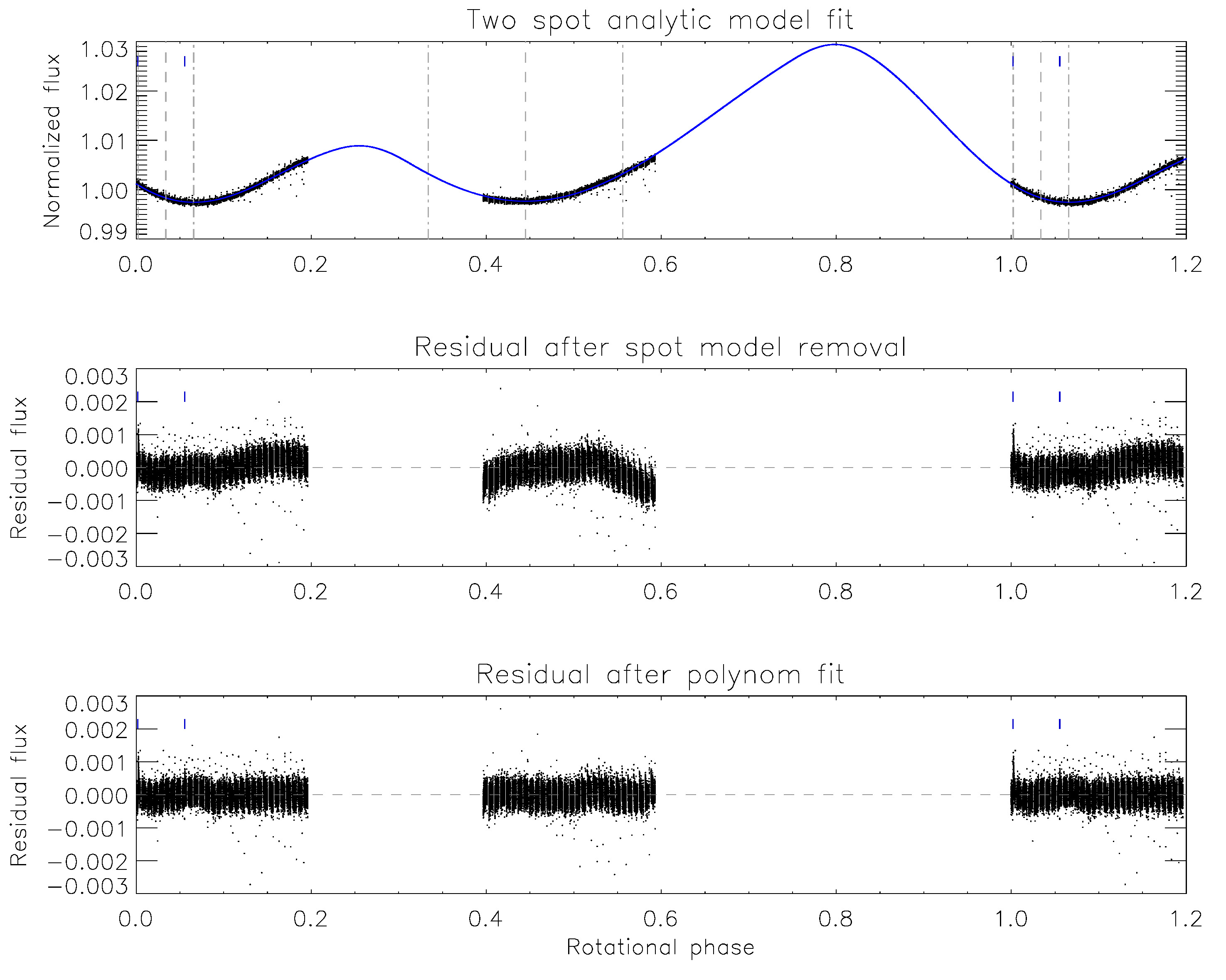
Figure 1: Analytical spot model fitted to our CHEOPS data. Upper panel: CHEOPS light curve (black dots) with the fitted analytic spot model (blue solid line). Dashed lines denote the longitudes of the fitted spots while dash-dotted lines indicate the radii of these spots. Middle panel: Residual after subtraction of the spot model. Lower panel: Residual after subtraction of the low-order polynomial. Blue ticks denote the positions of the two observed flares. The light curve is phased following Eq. 1 with $P_{\mathrm{rot}}=10.39\,\mathrm{d}$

.

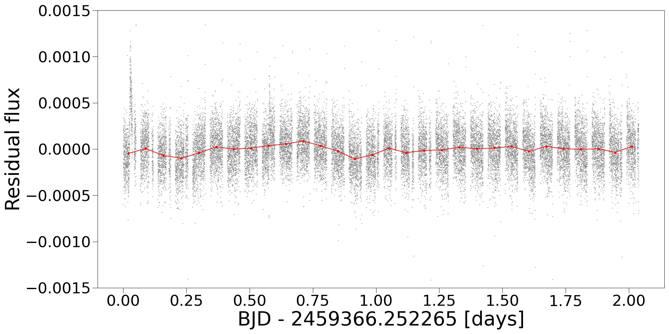
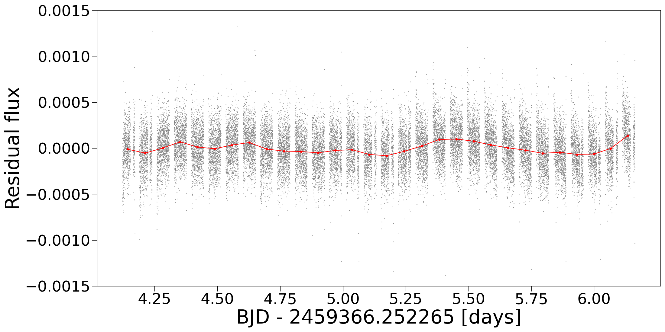
Figure 2: Residual light curves of the first (upper panel) and second (lower panel) visit to DE Boo after the subtraction of a fourth-order polynomial from the spot-model-subtracted data. Red dots show the orbital average flux for each orbit of CHEOPS. Red curves emphasise the change in the brightness of the target.

2.5 Estimating flare energies

During the first visit to DE Boo, two flares were detected by CHEOPS. This is the first time that flares have been photometrically observed and reported for DE Boo. This unprecedented detection justified a detailed analysis of these phenomena. In order to do so, we needed imagettes of sufficiently short cadence to resolve the finer structures of the flares. However, the resampling of these data for 15 seconds was also necessary to increase the S/N. The flares in the re-sampled imagette data are shown in Fig. 3.

In order to obtain the fraction of DE Boo’s quiescent luminosity in the CHEOPS band, a BT-NextGen model spectrum for a K0V-type star with T${}_{\mathrm{eff}}=$5300 K and logg$=4.5$ was convolved with the transmission curve of CHEOPS (Deline et al., 2020). Flare energies were then calculated by integrating the total flux for the duration of the flaring events, and multiplying them with the bolometric luminosity of DE Boo and the fraction of the luminosity in the CHEOPS band. Though we assumed that the flares originate from the primary, in reality they could arise from the M dwarf companion as well. However, as both the quiescent luminosity and the stellar spectrum are dominated by the K0V primary component, our approach is expected to provide a reasonable estimation of the flare energies. We note that the order of magnitude of the energies would not be different even if they originated from the companion.

3 Results

3.1 Improved radius of DE Boo

We improved existing measurements of the radius of DE Boo using a Markov-Chain Monte Carlo infrared flux method (MCMC IRFM; Blackwell & Shallis 1977; Schanche et al. 2020. This approach uses known relations between the stellar angular diameter, effective temperature, and apparent bolometric flux. For DE Boo, we computed the bolometric flux by constructing a spectral energy distribution (SED) of two stellar components: one of the primary using the spectral parameters derived above with the atlas catalogs (Castelli & Kurucz, 2003) and a second of the known M-dwarf companion with parameters taken from the phoenix catalogs (Allard et al., 2011). Empirical relations from Baraffe et al. (2015) were used to estimate the effective temperature and the radius of the companion. This was necessary in order to derive an accurate stellar radius for DE Boo using the derived parameters and the offset-corrected Gaia EDR3 parallax (Lindegren et al., 2021). We fitted the combined models to observed data taken from the most recent data releases for the following bandpasses: Gaia G, G_BP, and G_RP, 2MASS J, H, and K, and WISE W1 and W2 (Skrutskie et al., 2006; Wright et al., 2010; Gaia Collaboration et al., 2021). We used this fit to derive $R_{\star}=0.870\pm 0.021\,R_{\odot}$.

3.2 Properties of flare activity

We estimated the energies of the two flares observed during the first visit. The first, more energetic flare, which lasted for 20 minutes, occurred at the beginning of the observation period and had an estimated energy of 3.35$\times$10³² erg. In contrast, the second flare had a much shorter duration of 5 minutes and an energy of about 7.43$\times$10³¹ erg and was only identifiable on the imagettes. The detection of two flares with such energies under the total observation time of four days is not out of the ordinary on a fairly active late G or early K dwarf (e.g. Leitzinger et al. 2020, and references therein). The energy levels are relatively typical as well (Vida et al., 2021). Assuming that these flares originated from the companion, their energies would still be well within the boundaries of what is expected in the case of an M dwarf star. However, we note that two flares during a four-day period is not enough to make any quantitative conclusions about the flare activity. Derived parameters of the two flares along with their dates of occurrence are shown in Table 5.

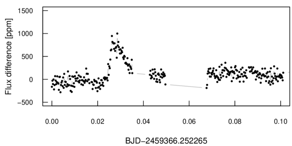
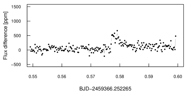
Figure 3: Two flares that occurred during the first visit to DE Boo, after re-sampling the imagette data to a cadence of 15 s.

Start date JD-2400000	End date JD-2400000	Duration $[min]$	Estimated energy $[erg]$
59366.273541	59366.287429	20	3.35$\times$1032
59366.830820	59366.834061	4.7	7.43$\times$1031

Table 5: Estimated energies and durations of the two flares during the first visit to DE Boo.

3.3 Possible photometric transients in the light-curve residuals

After masking out the flares, subtracting a spot model, and removing slowly varying systematic errors due to possible structures on the stellar surface that were not accounted for in our simple two-spot model, we noticed the presence of moderately slowly varying light-curve residuals on a timescale of 0.3–0.8 days. These residuals have a shorter timescale than what could be originated by the rotation of spots (and the timescale of spot emergence or decay is much longer than this; see e.g. Namekata et al. 2019), while the timescale is too long to be due to flares or other activity transients. Other typical light curve changes, such as ellipticity in closer binaries, or other tracers of magnetic activity typical of RS CVn systems are all related to rotation, and in our case would cause changes on longer timescales (see e.g. Berdyugina, 2005, and references therein). Therefore, we interpret these residuals as transients from the edge-on disk in the following.

Let us assume a cylindrically symmetric disk consisting of a light scattering material that follows some $\sigma(r,\phi)$ distribution. Here, $\sigma$ is the scattering cross section of the disk locally, that is, the fraction of starlight that is occulted or scattered by the dust particles in the elementary volume; $r$ is the radius vector, and $\phi$ is the angular coordinate. If the dust follows a circular orbit, the $\omega$ angular velocity can be expressed as $\omega=\sqrt{2GM}r^{-3/2}$, according to Kepler’s Third Law. Hence, during a $\rm{d}t$ time, we can write

$${\rm d}\phi=\omega{\rm d}t=\sqrt{2GM}\,r^{-\frac{3}{2}}\,{\rm d}t.$$ (3)

The variation of the disk scattering along the line of sight is then

$$\frac{{\rm d}\sigma}{{\rm d}t}=\frac{{\rm d}\sigma}{{\rm d}r}\frac{{\rm d}r}{{\rm d}t}+\frac{{\rm d}\sigma}{{\rm d}\phi}\frac{{\rm d}\phi}{{\rm d}t}=\frac{{\rm d}\sigma}{{\rm d}\phi}\sqrt{2GM}\,r^{-\frac{3}{2}}\,,$$ (4)

because $\frac{{\rm d}r}{{\rm d}t}=0$. The variation of the total scattering cross section along the line of sight $\Sigma=\int_{r1}^{r2}\sigma{\rm d}r$ can then be expressed as

$$\frac{{\rm d}\Sigma}{{\rm d}t}=\int_{r1}^{r2}\frac{{\rm d}\sigma}{{\rm d}\phi}\sqrt{2GM}\,r^{-\frac{3}{2}}\,{\rm d}r.$$ (5)

This formula represents the amount of material along a distinct line of sight. The light-curve transients are related to the transits of the individual grains along the stellar disk. If a material at $r$ radius with $\rho$ density scatters out a given fraction of the light $S$, the contribution to the light curve can be written as

$$S(r,t)=\left[\rho(r,\tau)\ast Lc(r,\tau)\right](t),$$ (6)

where $Lc$ is the transit light curve of a compact transiter at $r$ radius, $\ast$ denotes convolution, and $\tau$ is a running time-like variable, which was introduced because the transit light curve is a time-dependent variable itself. This expression shows that the shape of the transit light curve can be derived as the shapes of all individual overdensities at their $r$ radius and $\tau$ transit times combined appropriately and evaluated at t. If the configuration is very thin, and the scattered light is on the order of one part per thousand at most, the combination can be simplified to a summation. In this case, the combined effect of all contributions to the light curve shape will be written as

$$S(t)=\int_{R1}^{R2}\,\left[\rho(r,\tau)\ast Lc(r,\tau)\right](t)\,dr.$$ (7)

Here, the convolution shows that the frequency spectrum of the transit light curve will be the $F(\sigma)$ frequency spectrum belonging to the material distribution multiplied by the $F(T)$ frequency spectra of the transit light curves at different radii. If the cloud of grains is compact (the transiting structure is much smaller than the stellar disk) and $F(\sigma)$ includes components at very large frequencies, the boundary frequency in F(signal) will be the highest frequency in $F(T)$. If the transiting feature is compact, for example a small planet, the duration of the transient will be close to the transit duration. If the transiting feature is extended, for example a loose cloud of large asteroids or a giant comet, where the ingress and egress duration are compatible with (or even exceed) the transit duration, the experienced timescale of the transients will be significantly longer than the transit duration calculated at the orbital semi-major axis of the transiting feature.

If the transiting cloud is extended far beyond the stellar radius, $(\sigma)$ has only low-frequency components, and the observed light-curve anomaly will be very slow, on the order of $\Delta\phi/\sqrt{(2GM)}r^{-\frac{3}{2}}$. In this case, the smoothness of the distribution of the material and the orbital radius of the disk features become degenerate. Therefore, giving a lower limit for the orbital radius of the excess material, we also have to give an upper limit for its angular extension. Similar descriptions of these processes can be found in Kennedy et al. (2017).

In summary, the transit of the grains that generate a light-curve anomaly can be at most as long as the anomaly itself. Applying Kepler’s Third Law, this gives us an estimate, or more precisely, an upper limit of the radius where the claimed transiting features can be found, which we can write as

$$a_{max}=\frac{GM_{\star}D^{2}}{4(1-b^{2})R_{\star}^{2}},$$ (8)

where G is the gravitational constant, M_⋆ and R_⋆ are the mass and radius of DE Boo, respectively, $D$ is the duration of the light-curve anomaly itself, measured in units of time, and $b$ is the impact parameter, the projected distance of the transit chord from the center point of the star, measured in units of $R_{\star}$. If the shape of the transient is compatible with the transit of a compact, planet-like object, $D$ is related to the relative duration $W$, as $D=W\times P_{orb}$, where $W=R_{\star}/a\sqrt{(1+k)^{2}-b^{2}}/\pi$. If the light variation is more fuzzy and we cannot define a major transit bin, $D$ is to be understood as simply the time from the beginning to the end of the negative transit anomalies.

The residuals of the DE Boo observations are plotted in Fig. 2. The residuals of the two visits differ from each other. The first visit is compatible with a stable residual, with the dips suggesting one or two transients passing in front of the star. The most stable part of the residual is observed between 2459367.3 and 2459368.3. The second CHEOPS visit is merely composed of varying residuals and suggests density variations around the star rather than one transiting object. The most significant deviations from a constant residual are observed between 2459367.0 and 2459367.3, 2459370.8 and 2459371.6, and 2459371.75 and 2459372.35. Therefore, the experienced timescale of the suspected transients in the DE Boo light curve is 0.3–0.8 days.

Using the stellar parameters given in Table 1 and inserting 0.3 and 0.8 days for the transit duration into Eq. 8 and assuming $b=0$, we get 0.35 and 2.47 AU for the maximum orbital distance of the transiting feature. This places the transiting object much closer to the star than the debris disk, to indicatively 1 AU from DE Boo. The suspected structure is consistent with the criteria of dynamical stability according to Holman & Wiegert (1999). This criterion tells us that circumbinary structures farther from the system center than the $a_{c}$ critical radius are stable in the long term; whereas values of $a_{c}$ were found by means of numerical simulations and as a function of the $\mu$ mass ratio and the eccentricity of the binary. Table 7 in Holman & Wiegert (1999) shows us that near $\mu=$0.4–0.5, $e=0.5$ and $a_{c}$=3.6–3.7 if measured in the unit of the primary-to-secondary separation. As this separation is 0.19 AU, debris structures behind the critical radius of $a_{c}=0.703$ AU can be dynamically stable. Therefore, a transient at $\leavevmode\nobreak\ 1$ AU from the barycenter is dynamically plausible. We also note that Trilling et al. (2007) review several other dynamical criteria, but these authors find the Holman & Wiegert (1999) criterion to be the strictest of these, and therefore we applied the Holman & Wiegert (1999) criterion here.

4 Discussion and conclusions

We carried out photometric observations of DE Boo using the CHEOPS space telescope with a total duration of four days. In order to properly remove the effect of stellar variation, a stellar spot model and a fourth-order polynomial were fitted and subtracted from the light curves, respectively. We observed two flares during the observation period. This was the first time that flaring activity of DE Boo was reported. We found the estimated energies of the flares to be consistent with the predicted levels of activity of a magnetically active K dwarf star. We conclude that further measurements are required to obtain quantitative results about the stellar activity of DE Boo.

Local Thermodynamic Equilibrium (LTE) synthetic spectra were fitted to the observations taken with the echelle spectrograph mounted on the 1m RCC telescope at Piszkéstető, Hungary, and with SOPHIE installed on the 1.93m telescope at the Observatoire de Haute-Provence, France, in order to refine the astrophysical parameters of the primary. The two fits yielded the same results within their respective error bars.

Nonperiodic transiting features with a duration of 0.3–0.8 days were identified in the residual light curves of DE Boo. Based on their transit duration, the semi-major axes of these features were estimated. Our calculations show that these features had a maximum orbital distance of 2.47 AU. This is a much smaller value than the indicated inner radius of the debris disk that is seen in the infrared wavelengths. As the duration of our observations was less than the expected transit duration of the material passing in the debris disk at 70 AU according to Eq. 8 (around 4.5 days), it is not possible to detect their effects on the investigated light curves. Space telescopes with longer observational baselines (such as TESS) are better suited to this task. Moreover, we note that any effect with the duration of a few days was removed during the polynomial fitting. However, the goal of this study was not simply to identify features of an already known debris disk. As it is not out of the ordinary that an inner disk is found in a system with outer debris disks, it cannot be excluded that, for DE Boo, transiting material is observed much closer to the star than the most massive parts of the debris disk. In the case of $\beta$ Pic, we see a similar geometry: although the visible debris disk extends to 100 (secondary disk) and   200 (primary disk) AU, the observed transients last for less than a day, indicating that the presumed exocomets orbit much closer than the debris disks. Several systems with warm debris disks have also been known to exhibit quasi-periodic dippers with a timescale of 1–4 days; these were found to be due to transits of overdensities in the disk, of surprisingly large amplitude on some occasions (Tajiri et al., 2020). These systems are more similar to DE Boo in terms of the origin of the light variations. In these systems, the overdensities also appear in a structure that is close to the star (as can be concluded from their quasi-period), while the major warm debris disk lies much farther out.

A possible explanation for the observed light variations is the formation of an inner disk region, indicating ongoing dust replenishment Wahhaj et al. (2003), which can have an origin in the planetesimal belts Okamoto et al. (2004). Warm debris disks around evolved stars cannot be primary remnants of planet formation, but formed quite recently (Wyatt et al., 2007), most likely in a late heavy bombardment-like scenario, or from a very massive reservoir of planetesimals that survived planet formation (such as the Oort Cloud in the Solar System). In the presence of warm dust, excess radiation is expected in mid-infrared. However, no excess was detected at 24 $\mu$m by the Multiband Imaging Photometer for Spitzer (MIPS) for DE Boo (Gáspár et al., 2013). This may be because the detection limit of MIPS for debris disks at a distance of a few AU around late-type stars is above $f\sim 10^{-5}$. However, variations in the light curve of DE Boo imply a lower fractional luminosity, which is therefore below what may be detectable with MIPS. This suggests that the presence of a faint warm debris disk cannot be excluded.

The current observations covered 2$\times$2 days of DE Boo, and show that DE Boo is an important example of a system with an edge-on debris disk that we are looking at through the debris disk itself. Further observations with TESS in 2022, covering 28 days, will be an ideal opportunity to confirm our interpretations.

Appendix A Periodogram of spot-model-subtracted data

We applied the Lomb-Scargle periodogram to the spot-model-subtracted data from both visits before applying the fourth-order polynomial to check for remaining periods. Figure 4 shows the resulting periodogram, where the strongest peak was seen at 1.79 days. Another peak was present at around 100 minutes due to the orbital period of CHEOPS. We concluded that no higher harmonics of the stellar rotation of 10.39 days were present in the spot-model-subtracted data.

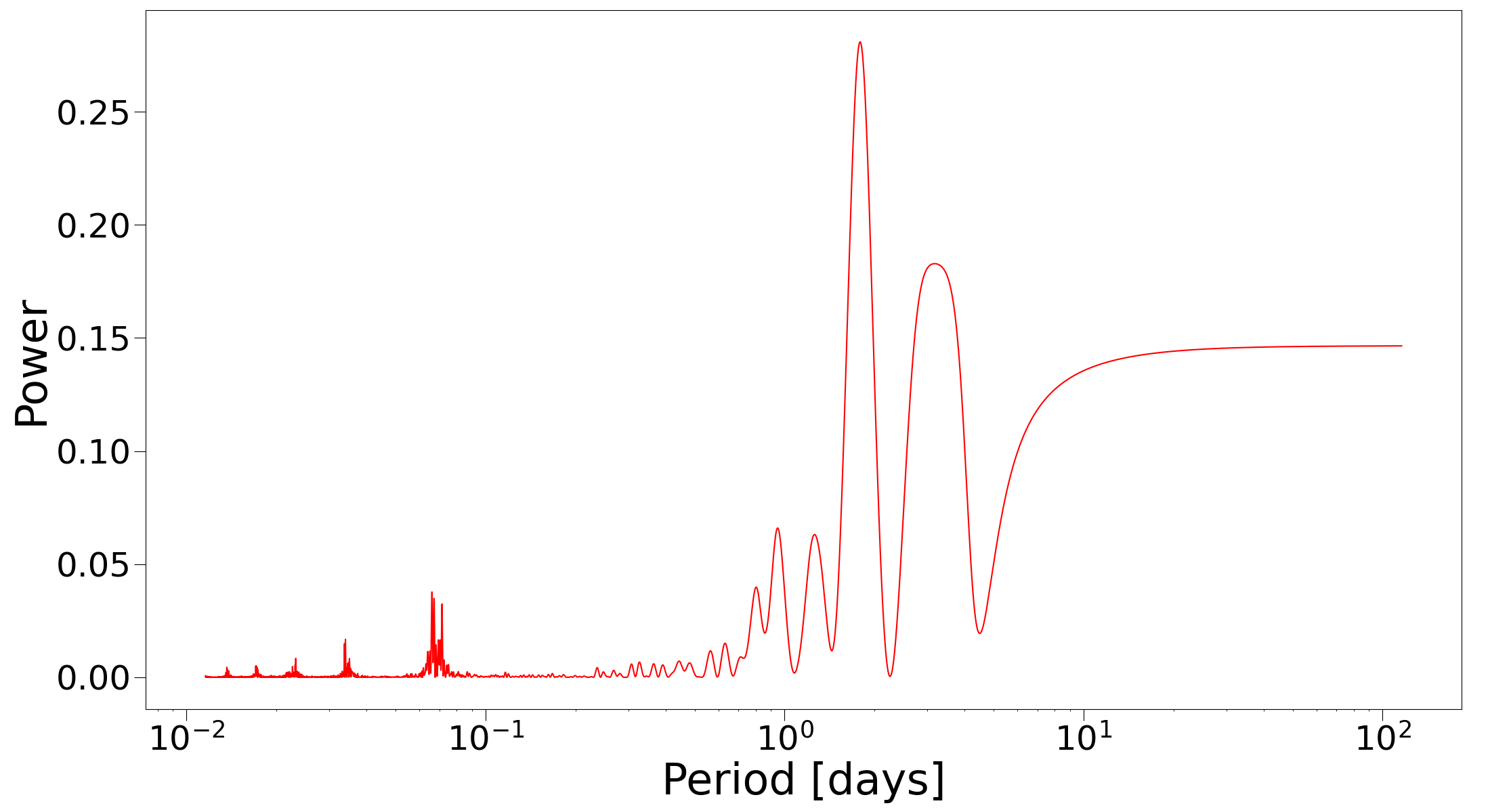
Figure 4: Lomb-Scargle periodogram of the spot-model-subtracted data. The peak with the maximum power belongs to the period of 1.79 days. We note that the effect of the 98.77 minute rotational period of CHEOPS also appears as a peak around 100 minutes.