Numerical study of a diffusion equation with Ventcel boundary condition using curved meshes

Abstract

In this work is provided a numerical study of a diffusion problem involving a second order term on the domain boundary (the Laplace-Beltrami operator) referred to as the Ventcel problem. A variational formulation of the Ventcel problem is studied, leading to a finite element discretization. The focus is on the resort to high order curved meshes for the discretization of the physical domain. The computational errors are investigated both in terms of geometrical error and of finite element approximation error, respectively associated to the mesh degree $r\geq 1$ and to the finite element degree $k\geq 1$. The numerical experiments we led allow us to formulate a conjecture on the a priori error estimates depending on the two parameters $r$ and $k$. In addition, these error estimates rely on the definition of a functional lift with adapted properties on the boundary to move numerical solutions defined on the computational domain to the physical one.

Keywords: Laplace-Beltrami operator, Ventcel boundary condition, finite element method, high order meshes, geometric error, a priori error estimates

Subject classification: 74S05, 65N15, 65N30, 65G99

Introduction

Motivation.

On the one hand, in various situations, we have to numerically solve a problem (a partial differential equation) on a non-polygonal geometry. This requires the use of high order meshes in order to well approximate it. On the other hand, in several industrial applications, objects or materials surrounded by a thin layer with potentially other properties (typically a surface treatment or corrosion) have to be considered. The presence of this layer causes some difficulties while discretizing the domain and numerically solving the problem. To overcome this problem, the domain is approximated asymptotically by an other one without a thin layer but equipped with artificial boundary conditions, like Ventcel boundary condition. The physical properties of the thin layer are then contained in the boundary condition.

This paper focuses on the resolution of a problem involving higher order boundary condition and numerically evaluates the a priori error produced by a finite element approximation on higher order meshes, distinguishing the geometrical error from the approximation error.

The Ventcel problem and its approximation.

Let $\Omega$ be a domain in $\mathbb{R}^{d}$, $d=2$, 3, with a smooth boundary $\Gamma$. The Laplace-Beltrami operator on $\Gamma$ is denoted by $\Delta_{\Gamma}$. Relatively to the source terms $f$ and $g$ and to the constants $\kappa\geq 0$, $\alpha,\,\beta>0$, the Ventcel problem reads,

$$\left\{\begin{aligned} -\Delta u+\kappa u&=&f&\quad\text{ in }\,\Omega,\\ -\beta\Delta_{\Gamma}u+\partial_{\boldsymbol{\mathrm{n}}}u+\alpha u&=&g&\quad\text{ on }\,\Gamma,\\ \end{aligned}\right.$$ (1)

with $\boldsymbol{\mathrm{n}}$ the external unit normal to $\Gamma$ and $\partial_{\boldsymbol{\mathrm{n}}}u$ the normal derivative of $u$ along $\Gamma$. The theoretical properties of the solution of problem (1) have been studied in [10].

Due to the presence of the second order term in the boundary condition, the domain $\Omega$ is required to be smooth and thus non-polygonal: from the numerical point of view, the computational domain $\Omega_{h}$ (the mesh domain) will not fit the physical one: $\Omega_{h}\neq\Omega$. In a context of finite element methods of high order $k\geq 2$, it then is necessary to resort to high order meshes of geometrical degree $r\geq 2$ to preserve the numerical solution’s accuracy. Some methods have been widely studied, see, e.g., [7, 6, 5, 14, 12].

The approximation of the Laplace equation on a surface has been studied in this framework by Demlow et al. in [3, 4]. In these works, a distinction is made between the geometrical error induced by the setting of the computational domain $\Omega_{h}\neq\Omega$ and the approximation error related to the finite element method. The purpose of this approach is to highlight the influence of the geometrical degree $r$ of the mesh and the finite element approximation degree $k$ on the total computational error. Thereby, one can assess which is the optimal degree of the finite element method $k$ to chose depending on the choice of the geometrical degree $r$.

In the present context where $\Omega_{h}\neq\Omega$, a crucial issue arises: how does one compare the numerical solutions $u_{h}$ to the exact one, in order to derive a priori error estimates? To circumvent this, a lift of $u_{h}$ onto $\Omega$ is defined: in [5], Dubois introduced such a lift based on the orthogonal projection onto the boundary $\Gamma$, which further was improved in terms of regularity by Elliott et al. [7]. This lift however does not fit the orthogonal projection on the computational domain boundary. An alternative definition is introduced in this paper which will be used to perform a numerical study of the computational error of problem (1).

Paper organization.

In section 1, after introducing some general mathematical tools, is stated and proven the well-posedness of the Ventcel problem (1). The following section 2 is devoted to the definition of the curved meshes of $\Omega$. In section 3 are presented the discretization of the Ventcel problem (1), the lift operator which is the keystone of the a priori error estimations and numerical experiments studying the method convergence rate depending on the mesh geometrical degree $r$ and on the finite element approximation degree $k$. The paper ends with a conclusion section presenting our conjecture on a priori error estimates.

1 Study of the Ventcel problem

Some mathematical tools.

Let us denote $\Omega$ a bounded connected open subset of $\mathbb{R}^{d}$ with a smooth boundary $\Gamma:=\partial{\Omega}$ at least of $\mathcal{C}^{2}$ regularity. The unit normal to $\Gamma$ pointing outwards is denoted by $\boldsymbol{\mathrm{n}}$. The classical spaces $\mathrm{L}^{2}(\Omega)$, $\mathrm{L}^{2}(\Gamma)$, $\mathrm{H}^{1}(\Omega)$ and $\mathrm{H}^{1}(\Gamma)$ are considered and we introduce the following Hilbert space and its associated norm (see [10, Lemma 2.5])

$$\mathrm{H}^{1}(\Omega,\Gamma):=\{u\in\mathrm{H}^{1}(\Omega),\ u_{|_{\Gamma}}\in\mathrm{H}^{1}(\Gamma)\},\qquad\|u\|^{2}_{\mathrm{H}^{1}(\Omega,\Gamma)}:=\|u\|^{2}_{\mathrm{H}^{1}(\Omega)}+\|u_{|_{\Gamma}}\|^{2}_{\mathrm{H}^{1}(\Gamma)}.$$

We consider the classical surface operators (see, e.g., [9, p. 192-196]):

• the tangential gradient of $u\in\mathrm{H}^{1}(\Gamma)$ is given by $\nabla_{\Gamma}u:=\nabla\tilde{u}-(\nabla\tilde{w}\cdot\boldsymbol{\mathrm{n}})\boldsymbol{\mathrm{n}}$, where $\tilde{u}\in\mathrm{H}^{1}(\mathbb{R}^{d})$ is any extension of $u$;

• the tangential divergence of $W\in\mathrm{H}^{1}(\Gamma,\mathbb{R}^{d})$ is $\mathrm{div}_{\Gamma}W:=\mathrm{div}\tilde{W}-(\mathrm{D}\tilde{W}\,\boldsymbol{\mathrm{n}})\cdot\boldsymbol{\mathrm{n}}$, where $\tilde{W}\in\mathrm{H}^{1}(\mathbb{R}^{d},\mathbb{R}^{d})$ is any extension of $W$ and $\mathrm{D}\tilde{W}$ is the differential of $\tilde{W}$;

• the Laplace-Beltrami operator of $u\in\mathrm{H}^{2}(\Gamma)$ is given by $\Delta_{\Gamma}u:=\mathrm{div}_{\Gamma}(\nabla_{\Gamma}u)$.

Finally, the following fundamental result is recalled, see, e.g., [2] and [8, §14.6].

Proposition 1.

Let $\Omega$ and $\Gamma=\partial\Omega$ be as stated previously. Let $\mathrm{d}:\mathbb{R}^{d}\to\mathbb{R}$ be the signed distance function with respect to $\Gamma$ defined by,

$$\mathrm{d}(x):=\left\{\begin{array}[]{ll}-\mathrm{dist}(x,\Gamma)&{\rm if}\,x\in\Omega,\\ 0&{\rm if}\,x\in\Gamma,\\ \mathrm{dist}(x,\Gamma)&{\rm otherwise},\end{array}\right.\qquad{\rm with}\quad\mathrm{dist}(x,\Gamma):=\inf\{|x-y|,\leavevmode\nobreak\ \ y\in\Gamma\}.$$

Then there exists a tubular neighborhood $\mathcal{U}_{\Gamma}$ of $\Gamma$ where $\mathrm{d}$ is a $\mathcal{C}^{2}$ function. Its gradient $\nabla\mathrm{d}$ is an extension of the external unit normal $\boldsymbol{\mathrm{n}}$ to $\Gamma$. Additionally, in this neighborhood $\mathcal{U}_{\Gamma}$, the orthogonal projection $b$ onto $\Gamma$ is uniquely defined and given by

$$b\,:\leavevmode\nobreak\ x\in\mathcal{U}_{\Gamma}\longmapsto b(x):=x-\mathrm{d}(x)\nabla\mathrm{d}(x)\in\Gamma.$$

Well-posedness of problem (1).

The weak form of (1) is to find $u\in\mathrm{H}^{1}(\Omega,\Gamma)$ such that,

$$\forall\ v\in\mathrm{H}^{1}(\Omega,\Gamma),\quad a(u,v)=l(v):=\int_{\Omega}fv\mathrm{d}x+\int_{\Gamma}gv\mathrm{d}\sigma,$$ (2)

where $a(\cdot,\cdot)$ is defined on $\mathrm{H}^{1}(\Omega,\Gamma)^{2}$ by:

$$a(u,v):=\int_{\Omega}\nabla u\cdot\nabla v\mathrm{d}x+\kappa\int_{\Omega}uv\mathrm{d}x+\beta\int_{\Gamma}\nabla_{\Gamma}u\cdot\nabla_{\Gamma}v\mathrm{d}\sigma+\alpha\int_{\Gamma}uv\mathrm{d}\sigma.$$ (3)

Notice that the weak form (2) is equivalent to the system introduced in (1) as it was proven in [10].

Theorem 1.

Let $\Omega$ and $\Gamma=\partial\Omega$ be as stated previously. Let $\alpha$, $\beta>0$, $\kappa\geq 0$, and $f\in\mathrm{L}^{2}(\Omega)$, $g\in\mathrm{L}^{2}(\Gamma)$. Then there exists a unique solution $u\in\mathrm{H}^{1}(\Omega,\Gamma)$ to problem (2).

The proof of this theorem is classical and is briefly given in [10, th. 3.2]. We detail it here for the sake of completeness. Let us notice that, additionally, it is proven in [10, th. 3.3] that there exists a (source term independent) constant $c>0$ such that

$$\|u\|_{\mathrm{H}^{2}(\Omega,\Gamma)}\leq c(\|f\|_{\mathrm{L}^{2}(\Omega)}+\|g\|_{\mathrm{L}^{2}(\Gamma)}).$$

Proof.

The proof relies on the Lax-Milgram theorem. The linear form $l(\cdot)$ in (2) and the bilinear form $a(\cdot,\cdot)$ in (3) being continuous respectively on $\mathrm{H}^{1}(\Omega,\Gamma)$ and on $\mathrm{H}^{1}(\Omega,\Gamma)^{2}$, it remains to show that $a$ is coercive. We must distinguish between two cases.

1) If $\kappa\neq 0$. The result is obvious: for all $u\in\mathrm{H}^{1}(\Omega,\Gamma)$, $a(u,u)\geq\min\{1,\kappa,\alpha,\beta\}\|u\|_{\mathrm{H}^{1}(\Omega,\Gamma)}^{2}$.

2) If $\kappa=0$. We proceed by contradiction assuming that there exists a sequence $(u_{n})_{n\in\mathbb{N}^{*}}$ in $\mathrm{H}^{1}(\Omega,\Gamma)$ such that for all $n\geq 1$,

$$\|\nabla u_{n}\|^{2}_{\mathrm{L}^{2}(\Omega)}+\beta\|\nabla_{\Gamma}u_{n}\|^{2}_{\mathrm{L}^{2}(\Gamma)}+\alpha\|u_{n}\|^{2}_{\mathrm{L}^{2}(\Gamma)}<\frac{1}{n}\big{(}\|u_{n}\|^{2}_{\mathrm{H}^{1}(\Omega)}+\|u_{n}\|^{2}_{\mathrm{H}^{1}(\Gamma)}\big{)}.$$

It follows that $u_{n}\neq 0$ for all $n\geq 1$. Thus $u_{n}$ can be renormalized such that $\|u_{n}\|_{\mathrm{H}^{1}(\Omega,\Gamma)}=1$ and it satisfies $\|\nabla u_{n}\|^{2}_{\mathrm{L}^{2}(\Omega)}+\beta\|\nabla_{\Gamma}u_{n}\|^{2}_{\mathrm{L}^{2}(\Gamma)}+\alpha\|u_{n}\|^{2}_{\mathrm{L}^{2}(\Gamma)}<\frac{1}{n}$. Therefore

$$\nabla u_{n}\to 0\ \ \ \mbox{ in }\ \mathrm{L}^{2}(\Omega),\quad\nabla_{\Gamma}u_{n}\to 0\ \ \ \mbox{ in }\ \mathrm{L}^{2}(\Gamma)\quad\mbox{ and }\quad u_{n}\to 0\ \ \ \mbox{ in }\ \mathrm{L}^{2}(\Gamma).$$ (4)

Since $(u_{n})_{n}$ is bounded in $\mathrm{H}^{1}(\Omega,\Gamma)$, there exists $u\in\mathrm{H}^{1}(\Omega,\Gamma)$ such that $u_{n}\rightharpoonup u$ in $\mathrm{H}^{1}(\Omega,\Gamma)$, and since ${\mathrm{H}^{1}(\Omega,\Gamma)\hookrightarrow\leavevmode\nobreak\ \mathrm{L}^{2}(\Omega,\Gamma)}$ is a compact injection, we obtain

$$u_{n}\to u\ \ \mbox{in}\ \ \mathrm{L}^{2}(\Omega,\Gamma).$$ (5)

Passing to the limit in $\|u_{n}\|^{2}_{\mathrm{H}^{1}(\Omega,\Gamma)}=\|\nabla u_{n}\|^{2}_{\mathrm{L}^{2}(\Omega)}+\|\nabla_{\Gamma}u_{n}\|^{2}_{\mathrm{L}^{2}(\Gamma)}+\|u_{n}\|^{2}_{\mathrm{L}^{2}(\Gamma)}+\|u_{n}\|^{2}_{\mathrm{L}^{2}(\Omega)}=1$, and using the convergences given in (4) and (5), we obtain $\|u\|^{2}_{\mathrm{L}^{2}(\Omega,\Gamma)}=1$. However, since $\nabla u_{n}\rightharpoonup\nabla u$ in $\mathrm{L}^{2}(\Omega)$, we use (4) and the uniqueness of the limit to obtain $\nabla u=0$ and, since $\Omega$ is a connected set, it follows that $u=C\in\mathbb{R}$. Finally, $u_{n}\to u$ in $\mathrm{L}^{2}(\Gamma)$ and also $u_{n}\to 0$ in $\mathrm{L}^{2}(\Gamma)$, these two points yield $u=0=C$ which contradicts $\|u\|_{\mathrm{L}^{2}(\Omega,\Gamma)}=1$ and concludes the proof of the coercivity. ∎

2 Curved mesh definition

In this section are defined curved meshes of geometrical degree $r\geq 1$ of the domain $\Omega$. From now on, the domain $\Omega\subset\mathbb{R}^{d}$, $d=$2 or 3, is assumed to be at least $\mathcal{C}^{r+2}$ regular, and $\hat{T}$ denotes the reference simplex of dimension $d$. The definition steps are the following (see [7, 14, 5] for more details).

1. Construct an affine mesh $\mathcal{T}_{h}^{(1)}$ of $\Omega$ composed of simplexes $T$.

2. For each $T\in\mathcal{T}_{h}^{(1)}$, a mapping $F_{T}^{(e)}:\leavevmode\nobreak\ \hat{T}\rightarrow{T}^{(e)}:=F_{T}^{(e)}(\hat{T})$ is designed, so that the exact element ${T}^{(e)}$ form a curved mesh $\mathcal{T}_{h}^{(e)}$ whose domain exactly fits $\Omega$.

3. For each $T\in\mathcal{T}_{h}^{(1)}$, the mapping $F_{T}^{(e)}$ is interpolated by a polynomial $F_{T}^{(r)}$ of degree $r$. The associated elements ${T}^{(r)}:=F_{T}^{(r)}(\hat{T})$ form a curved mesh $\mathcal{T}_{h}^{(r)}$ of degree $r$ of $\Omega$.

Affine mesh.

Let $\mathcal{T}_{h}^{(1)}$ be a mesh of $\Omega$ made of simplexes of dimension $d$ (triangles or tetrahedra), it is chosen as quasi-uniform and henceforth shape-regular (see [1, def. 4.4.13]). The mesh domain is denoted by $\Omega_{h}^{(1)}:=\cup_{T\in\mathcal{T}_{h}^{(1)}}T$ and its boundary by $\Gamma_{h}^{(1)}:=\partial\Omega_{h}^{(1)}$, which is composed of $(d-1)$-dimensional simplexes that form a mesh of $\Gamma=\partial\Omega$. The vertices of $\Gamma_{h}^{(1)}$ are assumed to lie on $\Gamma$. We define the mesh size $h:=\max\{{\rm diam}(T);T\in\mathcal{T}_{h}^{(1)}\}$. To each $T\in\mathcal{T}_{h}^{(1)}$ is associated an affine function $F_{T}:\hat{T}\to T=F_{T}(\hat{T})$.

Remark 1.

For a sufficiently small $h$, the mesh boundary satisfies $\Gamma_{h}^{(1)}\subset\mathcal{U}_{\Gamma}$, where $\mathcal{U}_{\Gamma}$ is the tubular neighborhood given in proposition 1. This guaranties that the orthogonal projection $b:\Gamma_{h}^{(1)}\rightarrow\Gamma$ is one to one which is required for the construction of the exact mesh.

Example 1.

In the two dimensional case is displayed the case of a triangle $T\in\mathcal{T}_{h}^{(1)}$, with $T\cap\Gamma=\{v_{1},v_{2}\}$, together with the mapping $F_{T}$ that maps $\hat{T}$ into $T$.

Exact mesh $\mathcal{T}_{h}^{(e)}$.

After the early works of Scot [14] and Lenoir [11] defining transformations towards curved elements, Dubois [5] first introduced a definition based on the orthogonal projection $b$ onto $\Gamma$, further developed by Elliott et al. [7, §4] in terms of regularity, which definition is recalled here.

Let us first point out that, because of the quasi uniform assumption made on the mesh $\mathcal{T}_{h}^{(1)}$, and for $h$ sufficiently small, a mesh element $T$ cannot have $d+1$ vertices on the boundary $\Gamma$. We define internal elements as those having at most one vertex on the boundary $\Gamma$, whereas other elements have:

• 2 vertices on the boundary in the two dimensional case;

• 2 or 3 vertices on $\Gamma$ in the 3D case, forming either an edge or a face respectively.

The case of internal elements is skipped by setting $F_{T}^{(e)}=F_{T}$.

Let then $T\in\mathcal{T}_{h}^{(1)}$ a non-internal element, denote $v_{i}=F_{T}(\hat{v}_{i})$ its vertices, $\hat{v}_{i}$ being the vertices of $\hat{T}$, and define $\varepsilon_{i}=1$ if $v_{i}\in\Gamma$ or $\varepsilon_{i}=0$ otherwise. To $\hat{x}\in\hat{T}$ is associated its barycentric coordinates $\lambda_{i}$ associated to the vertices $\hat{v}_{i}$ of $\hat{T}$ . We introduce $\lambda^{\star}:=\sum_{i=1}^{d+1}\varepsilon_{i}\lambda_{i}$ and $\hat{y}:=\dfrac{1}{\lambda^{\star}}\sum_{i=1}^{d+1}\varepsilon_{i}\hat{v}_{i}\in\hat{T}$. The mapping $F_{T}^{(e)}:\leavevmode\nobreak\ \hat{T}\rightarrow{T}^{(e)}$ is given by,

$$F_{T}^{(e)}(\hat{x}):=x+(\lambda^{\star})^{r+2}(b(y)-y),\quad{\rm with}\quad x=F_{T}(\hat{x})\quad{\rm and}\quad y=F_{T}(\hat{y}).$$ (6)

Remark 2.

For $x\in T\cap\Gamma_{h}$, we have that $\lambda^{\star}=1$ and so $y=x$ inducing that $F_{T}^{(e)}(\hat{x})=b(x)$: $F_{T}^{(e)}\circ F_{T}^{-1}=b$ on $T\cap\Gamma_{h}$ which is then mapped on $\Gamma$ following the orthogonal projection $b$. The mapping $F_{T}^{(e)}$ has been shown in [7] to be $C^{r+1}$ regular on $\hat{T}$.

Example 2.

Consider three triangles $T_{1}$, $T_{2}$ and $T_{3}$ in $\mathbb{R}^{2}$ as displayed below. For $i=1,2,3$, we have the following transformation $F_{T_{i}}^{(e)}\circ F_{T_{i}}^{-1}$ that maps $T_{i}\in\mathcal{T}_{h}^{(1)}$ into ${T}^{(e)}_{i}$ as follows,

$T_{1}$ and $T_{2}$ are internal and so are unchanged whereas $T_{3}$ (having 2 vertices on $\Gamma$) is not internal and mapped into a curved triangle with an edge exactly fitting $\Gamma$.

Curved mesh $\mathcal{T}_{h}^{(r)}$ with degree $r$.

Let $T\in\leavevmode\nobreak\ \mathcal{T}_{h}^{(1)}$ and $r\geq 1$, the exact mapping $F_{T}^{(e)}$ in (6) is interpolated as a polynomial of degree $r$ in the classical $\mathbb{P}^{r}$-Lagrange basis on $\hat{T}$. The interpolant is denoted by $F_{T}^{(r)}$ and we define ${T}^{(r)}:=F_{T}^{(r)}(\hat{T})$. The curved mesh of degree $r$ is $\mathcal{T}_{h}^{(r)}:=\{{T}^{(r)};T\in\mathcal{T}_{h}^{(1)}\}$ with domain $\Omega_{h}^{(r)}:=\cup_{{T}^{(r)}\in\mathcal{T}_{h}^{(r)}}{T}^{(r)}$ and with boundary $\Gamma_{h}^{(r)}:=\partial\Omega_{h}^{(r)}$. Note that $F_{T}^{(r)}(v)=F_{T}^{(e)}(v)$ for $v$ a $\mathbb{P}^{r}$-Lagrange node in $\hat{T}$.

Example 3.

In the quadratic case $r=2$ is displayed a border quadratic element $T^{(2)}$. The mappings $F_{T}^{(2)}$ and $F_{T}^{(e)}$ coincide at the $\mathbb{P}^{2}$-Lagrange nodes which are the three vertexes $\hat{v}_{i}$ and the three edge mid-points $\hat{e}_{i}$ of $\hat{T}$.

3 Numerical experiments

Functional lift.

Here, we define lifts to transform a function on a domain $\Omega_{h}^{(r)}$ or $\Gamma_{h}^{(r)}$ (defined in the previous section) into a function defined on $\Omega$ or $\Gamma$ respectively. Lifts are necessary for two reasons: to compare the numerical solutions to the exact one and thus perform a priori error estimates, but also to define the right hand side source terms in the numerical formulation of problem (1).

A surface lift is obviously provided by the orthogonal projection $b:\leavevmode\nobreak\ \Gamma_{h}^{(r)}\rightarrow\Gamma$, to $v_{h}\in{\rm L}^{2}(\Gamma_{h}^{(r)})$ is associated $v_{h}^{L}\in{\rm L}^{2}(\Gamma)$ given by $v_{h}^{L}\circ b=v_{h}$.

To define a volume lift, a transformation $G_{h}^{(r)}:\leavevmode\nobreak\ \Omega_{h}^{(r)}\rightarrow\Omega$ is defined and then to $u_{h}\in{\rm L}^{2}(\Omega_{h}^{(r)})$ is associated $u_{h}^{\ell}\in{\rm L}^{2}(\Omega)$ given by $u_{h}^{\ell}\circ G_{h}^{(r)}=u_{h}$. The definition of $G_{h}^{(r)}$ is less obvious and we describe it here.

In [7], it is given piecewise on all ${T}^{(r)}\in\mathcal{T}_{h}^{(r)}$ by ${G_{h}}_{|_{{T}^{(r)}}}:=F_{T}^{(e)}\circ({F_{T}^{(r)}})^{-1}$, where $T$ is the affine element relative to ${T}^{(r)}$. However, this transformation does not fit the orthogonal projection $b$ on the mesh boundary. Precisely, following remark 2, for $x\in\Gamma_{h}^{(r)}\cap{T}^{(r)}$, $G_{h}(x):=b\circ F_{T}\circ({F_{T}^{(r)}})^{-1}(x)$. As a result the surface and bulk lifts do not coincide on $\Gamma_{h}^{(r)}$: $\left({\rm Tr}\leavevmode\nobreak\ u_{h}\right)^{L}\neq{\rm Tr}(u_{h}^{\ell})$.

To avoid this, we propose the following alternative definition of $G_{h}^{(r)}$ that is given piecewise for all ${T}^{(r)}\in\mathcal{T}_{h}^{(r)}$ by (with the notations of equation (6)),

$${G_{h}^{(r)}}_{|_{{T}^{(r)}}}:=F_{T^{(r)}}^{(e)}\circ({F_{T}^{(r)}})^{-1},\quad F_{T^{(r)}}^{(e)}(\hat{x}):=x+(\lambda^{\star})^{r+2}(b(y)-y),$$ (7)

with $x=F_{T}^{(r)}(\hat{x})$ and $y=F_{T}^{(r)}(\hat{y}).$ Geometrically, ${T}^{(r)}$ is directly transformed into ${T}^{(e)}$ by $F_{T^{(r)}}^{(e)}\circ(F_{T}^{(r)})^{(-1)}$, without being first transformed into $T$ as previously done. Now, for $x\in F_{T}^{(r)}\cap\Gamma_{h}^{(r)}$, $\hat{x}=(F_{T}^{(r)})^{(-1)}(x)$ satisfies $\lambda^{\star}=1$ and so $\hat{y}=\hat{x}$ and $y=x$. So $F_{T^{(r)}}^{(e)}(\hat{x})=b(x)$, the volume and surface lifts both coincide with $b$ on $\Gamma_{h}^{(r)}$ and the expected relation,

$$\forall\leavevmode\nobreak\ u_{h}\in{\rm H}^{1}(\Omega_{h}^{(r)}),\quad\left({\rm Tr}\leavevmode\nobreak\ u_{h}\right)^{L}={\rm Tr}(u_{h}^{\ell}),$$

now holds. Consequently, the surface lift $v_{h}^{L}$ now simply will be denoted by $v_{h}^{\ell}$.

Finite element formulation and implementation.

On a mesh $\mathcal{T}_{h}^{(r)}$ is considered the finite element space,

$$V_{h}:=\left\{u\in{\rm C}^{0}(\Omega_{h}^{(r)}),\leavevmode\nobreak\ \forall\leavevmode\nobreak\ T\in\mathcal{T}_{h}^{(r)},\leavevmode\nobreak\ u_{|T}\circ F_{T}^{(r)}\in\mathbb{P}^{k}(\hat{T})\right\},$$ (8)

with $\mathbb{P}^{k}(\hat{T})$ the polynomials of degree $k$ on $\hat{T}$ and with $k\geq 1$ the finite element degree. Following [7], the problem (1) is discretized as: find $u_{h}\in V_{h}$ such that,

$$\forall v_{h}\in V_{h},\quad a_{h}(u_{h},v_{h})=l_{h}(v_{h}):=\int_{\Omega_{h}^{(r)}}f^{-\ell}\,J_{G_{h}^{(r)}}\mathrm{d}x+\int_{\Gamma_{h}^{(r)}}g^{-\ell}\,J_{b}\mathrm{d}\sigma,$$ (9)

with $G_{h}^{(r)}$ defined in (7), with $f^{-\ell}:=f\circ G_{h}^{(r)}$ and $g^{-\ell}:=g\circ b$ the inverse lifts of the source terms in (1), with $J_{G_{h}^{(r)}}$ and $J_{b}$ the Jacobians of $G_{h}^{(r)}$ and $b_{\Gamma_{h}^{(r)}}$ respectively and where $a_{h}$ is the bilinear form in (3) rewritten on $\Omega_{h}^{(r)}$ and $\Gamma_{h}^{(r)}$.

Finite element space definition, matrix assembling and computation on curved surfaces are led using the code Cumin [13]. All integral computations rely on quadrature rules on the reference elements which are always chosen of sufficient order without further details.

Laplace equation on a surface.

In order to validate the code, we first draw our attention towards the Laplace equation $-\Delta_{\Gamma}u+u=g$ on a smooth surface $\Gamma\subset\mathbb{R}^{3}$. We refer to Demlow [3, 4] for the analysis of its finite element formulation. Given a mesh $\mathcal{T}_{h}^{(r)}$ of $\Gamma$, following (8), the $\mathbb{P}^{k}$-Lagrange finite element space is $W_{h}:=\left\{u\in{\rm C}^{0}(\Gamma_{h}^{(r)}),\leavevmode\nobreak\ \forall\leavevmode\nobreak\ T\in\mathcal{T}_{h}^{(r)},\leavevmode\nobreak\ u_{|T}\circ F_{T}^{(r)}\in\mathbb{P}^{k}(\hat{T})\right\}$ and the discrete problem is: find $u_{h}\in W_{h}$ such that,

$$\forall\leavevmode\nobreak\ v_{h}\in W_{h},\quad\int_{\Gamma_{h}^{(r)}}\nabla_{T}u_{h}\cdot\nabla_{T}v_{h}\,\mathrm{d}\sigma+\int_{\Gamma_{h}^{(r)}}u_{h}\,v_{h}\,\mathrm{d}\sigma=\int_{\Gamma_{h}^{(r)}}v_{h}\,g^{-\ell}\,J_{b}\,\mathrm{d}\sigma,$$

with $g^{-\ell}$ and $J_{b}$ previously defined in (9). The a priori error estimate for this problem developed by Demlow reads,

$$\|u-u_{h}^{\ell}\|_{\mathrm{L}^{2}(\Gamma)}=O(h^{k+1}+h^{r+1}),\quad\|\nabla_{\Gamma}(u-u_{h}^{\ell})\|_{\mathrm{L}^{2}(\Gamma)}=O(h^{k}+h^{r+1}),$$ (10)

for a smooth enough source term $g$.

We set $\Gamma$ to the unit sphere and the source term to $g(x,y,z)=\mathrm{e}^{y}(y+2)y$. Three series of successively refined meshes, respectively affine, quadratic and cubic, of $\Gamma$ have been generated by the software Gmsh. The numerical errors have been computed for each mesh and for $\mathbb{P}^{k}$, with $k=1,\dots 4$.

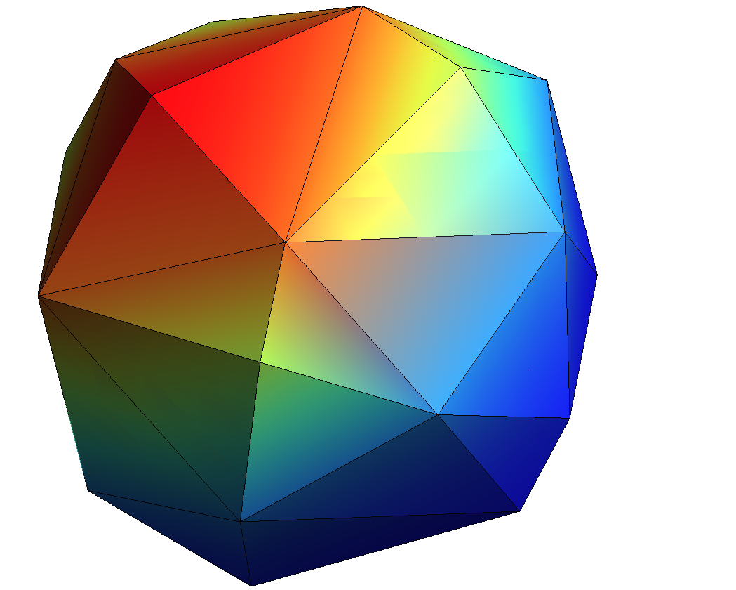
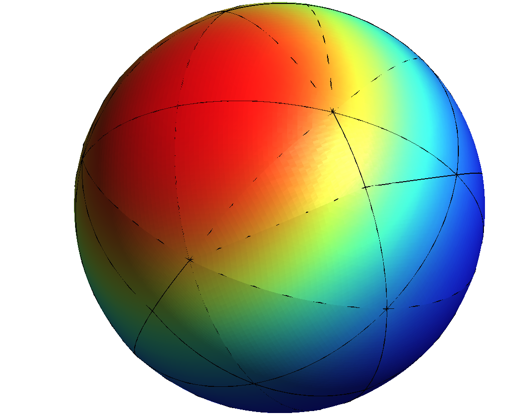
Figure 1: Numerical solution of the Laplace equation on a sphere with affine and quadratic meshes.

	$\|u-u_{h}^{\ell}\|_{\mathrm{L}^{2}(\Gamma)}$				$\|u-u_{h}^{\ell}\|_{\mathrm{H}^{1}(\Gamma)}$
	$\mathbb{P}^{1}$	$\mathbb{P}^{2}$	$\mathbb{P}^{3}$	$\mathbb{P}^{4}$	$\mathbb{P}^{1}$	$\mathbb{P}^{2}$	$\mathbb{P}^{3}$	$\mathbb{P}^{4}$
Affine mesh (r=1)	1.96	1.96	1.96	1.96	0.99	1.96	1.96	1.96
Quadratic mesh (r=2)	1.98	2.95	3.92	3.92	0.98	1.97	3.00	3.91
Cubic mesh (r=3)	1.98	2.94	3.95	3.92	0.98	1.96	2.96	3.95

Table 1: Convergence order for the Laplace equation on a sphere.

The numerical solution on two coarse meshes is depicted on figure 1, and the measured convergence orders are reported in table 1. The affine and cubic meshes behave exactly as expected following (10). In turn, quadratic meshes produce unexpected convergence rates indicated in red in table 1 and a super convergence is observed. Quadratic meshes display a geometrical error $h^{4}$ instead of the expected $h^{3}$ and thus behave as if $r=3$. This behavior has been further investigated and is not problem dependent. It is also observed for the Poisson problem on a disk with Neumann or Robin boundary conditions. It is neither caused by the considered geometry: studying a simpler problem of integral computation on a non-symmetric and non-convex domain gave the same surprising super convergence. So far we have no further explanation for this particular error.

Numerical study of the Ventcel problem.

The Ventcel problem (1) is considered on the unit disk $\Omega$ with $\alpha=\beta=1$ and $\kappa=0$, with the source terms $f(x,y)=-y\mathrm{e}^{x}$ and $g(x,y)=y\mathrm{e}^{x}(3+4x-y^{2})$ corresponding to the exact solution $u=-f$. The discrete problem (9) is implemented and solved using the code Cumin [13]. Again, three series of successively refined meshes, respectively affine, quadratic and cubic, of $\Omega$ have been generated with Gmsh. For each mesh and for $\mathbb{P}^{k}$ finite elements, with $k=1\dots 4$, four numerical errors are computed (two in the bulk domain and two on the boundary),

$$\|u-u_{h}^{\ell}\|_{\mathrm{L}^{2}(\Omega)},\quad\|\nabla(u-u_{h}^{\ell})\|_{\mathrm{L}^{2}(\Omega)},\quad\|u-u_{h}^{\ell}\|_{\mathrm{L}^{2}(\Gamma)}\quad{\rm and}\quad\|\nabla_{\Gamma}(u-u_{h}^{\ell})\|_{\mathrm{L}^{2}(\Gamma)},$$

and the estimated convergence rates are reported in the two tables 2 and 3.

	$\|u-u_{h}^{\ell}\|_{\mathrm{L}^{2}(\Gamma)}$				$\|\nabla_{\Gamma}(u-u_{h}^{\ell})\|_{\mathrm{L}^{2}(\Gamma)}$
	$\mathbb{P}^{1}$	$\mathbb{P}^{2}$	$\mathbb{P}^{3}$	$\mathbb{P}^{4}$	$\mathbb{P}^{1}$	$\mathbb{P}^{2}$	$\mathbb{P}^{3}$	$\mathbb{P}^{4}$
Affine mesh (r=1)	2.00	2.03	2.01	2.01	1.00	2.00	1.99	1.98
Quadratic mesh (r=2)	2.00	3.00	4.00	4.02	1.00	2.00	3.00	4.02
Cubic mesh (r=3)	2.00	3.00	4.00	4.24	1.00	2.00	3.00	3.98

Table 2: Convergence order of $\|u-u_{h}^{\ell}\|_{\mathrm{L}^{2}(\Gamma)}$ and of $\|\nabla_{\Gamma}(u-u_{h}^{\ell})\|_{\mathrm{L}^{2}(\Gamma)}$

The surface errors in table 2 behave exactly the same way as the estimation (10) for the Laplace equation on a surface: the same super-convergence for the quadratic meshes again occurs, as if $r=3$ in that case. As a consequence, the numerical solution seems to be correctly computed.

	$\|u-u_{h}^{\ell}\|_{\mathrm{L}^{2}(\Omega)}$				$\|\nabla(u-u_{h}^{\ell})\|_{\mathrm{L}^{2}(\Omega)}$
	$\mathbb{P}^{1}$	$\mathbb{P}^{2}$	$\mathbb{P}^{3}$	$\mathbb{P}^{4}$	$\mathbb{P}^{1}$	$\mathbb{P}^{2}$	$\mathbb{P}^{3}$	$\mathbb{P}^{4}$
Affine mesh (r=1)	1.98	1.99	1.97	1.97	1.00	1.50	1.49	1.49
Quadratic mesh (r=2)	2.01	3.14	3.94	3.97	1.00	2.12	3.03	3.48
Cubic mesh (r=3)	2.04	2.45	3.44	4.04	1.02	1.47	2.42	3.46

Table 3: Convergence order of $\|u-u_{h}^{\ell}\|_{\mathrm{L}^{2}(\Omega)}$ and $\|\nabla(u-u_{h}^{\ell})\|_{\mathrm{L}^{2}(\Omega)}$

The interpretation of the convergence rates for the bulk errors in table 3 is less straightforward. Let us first focus on the affine and quadratic meshes, and consider that in the quadratic case $r=3$ instead of $2$ (as a consequence of the super convergence in that case previously discussed). Then the figures in table 3 can be interpreted as,

$$\|u-u_{h}^{\ell}\|_{\mathrm{L}^{2}(\Omega)}=O(h^{k+1}+h^{r+1})\quad{\rm and}\quad\|\nabla(u-u_{h}^{\ell})\|_{\mathrm{L}^{2}(\Omega)}=O(h^{k}+h^{r+1/2}).$$

This behavior differs from (10) for the gradient norm where $h^{r+1}$ is now replaced by $h^{r+1/2}$. This difference could be understood from a theoretical point of view following ideas that should be presented in fore coming works.

For the cubic case, the $\mathbb{P}^{1}$ and $\mathbb{P}^{4}$ cases behave the same way. However, for the $\mathbb{P}^{2}$ and $\mathbb{P}^{3}$ cases (red figures in table 3), the rule rather seem to be $\|u-u_{h}^{\ell}\|_{\mathrm{L}^{2}(\Omega)}=O(h^{k+1/2}+h^{r+1})$ and $\|\nabla u-\nabla u_{h}^{\ell}\|_{\mathrm{L}^{2}(\Omega)}=O(h^{k-1/2}+h^{r+1/2})$. Though we have no clear understanding on this, we experienced that the choice of the lift operator here has a crucial influence. We recall that this lift is based on a geometric transformation $G_{h}^{(r)}:\leavevmode\nobreak\ \Omega_{h}^{(r)}\rightarrow\Omega$, which is a modification of the one defined in [7]. When resorting to the lift in [7], a saturation of the convergence order is observed: 2.5 for the $\mathrm{L}^{2}(\Omega)$ norm and 1.5 for the gradient $\mathrm{L}^{2}$-norm on $\Omega$. The same observation holds both for the quadratic and cubic meshes.

Conclusion

We have presented an approach in order to numerically solve the Ventcel problem (1) and have used the code Cumin [13] to give a numerical exploration of the associated a priori errors using high order finite elements on curved meshes. This numerical analysis is supported by an alternative definition of a lift operator as compared to the previous work [7] which improved our numerical results. Beyond difficulties related to the lift definition, and beyond unexplained super convergence associated to quadratic meshes, we formulate the following conjecture for the Ventcel problem a priori numerical errors, the proof of which is a work in progress.
Conjecture. Let $u\in\mathrm{H}^{k+1}(\Omega,\Gamma)$ be a solution of the variational problem (2), let $\mathcal{T}_{h}^{(r)}$ be a mesh of $\Omega$ with geometrical degree $r$, let $V_{h}$, defined in (8), be the associated finite element space of degree $k$. Then the numerical solution $u_{h}\in V_{h}$ to the discrete problem (9) satisfies,

$$\|u-u_{h}^{\ell}\|_{\mathrm{L}^{2}(\Omega)}=O(h^{k+1}+h^{r+1}),\quad\quad\quad\leavevmode\nobreak\ \|\nabla(u-u_{h}^{\ell})\|_{\mathrm{L}^{2}(\Omega)}=O(h^{k}+h^{r+1/2}),$$

$$\|u-u_{h}^{\ell}\|_{\mathrm{L}^{2}(\Gamma)}=O(h^{k+1}+h^{r+1}),\quad{\rm and}\quad\|\nabla_{\Gamma}(u-u_{h}^{\ell})\|_{\mathrm{L}^{2}(\Gamma)}=O(h^{k}+h^{r+1}).$$

References

- [1] S. C. Brenner and L. R. Scott. The mathematical theory of finite element methods. 15:16,361, 2002.
- [2] C. Dapogny and P. Frey. Computation of the signed distance function to a discrete contour on adapted triangulation. Calcolo, 49(3):193–219, 2012.
- [3] A. Demlow. Higher-order finite element methods and pointwise error estimates for elliptic problems on surfaces. SIAM J. Numer. Anal., 47(2):805–827, 2009.
- [4] A. Demlow and G. Dziuk. An adaptive finite element method for the Laplace-Beltrami operator on implicitly defined surfaces. SIAM J. Numer. Anal., 45(1):421–442, 2007.
- [5] F. Dubois. Discrete vector potential representation of a divergence-free vector field in three-dimensional domains: numerical analysis of a model problem. SIAM J. Numer. Anal., 27(5):1103–1141, 1990.
- [6] D. Edelmann. Isoparametric finite element analysis of a generalized Robin boundary value problem on curved domains. SMAI J. Comput. Math., 7:57–73, 2021.
- [7] C. M. Elliott and T. Ranner. Finite element analysis for a coupled bulk-surface partial differential equation. IMA J. Numer. Anal., 33(2):377–402, 2013.
- [8] D. Gilbarg and N. S. Trudinger. Elliptic partial differential equations of second order. Classics in Mathematics. Springer-Verlag, Berlin, 2001. Reprint of the 1998 edition.
- [9] A. Henrot and M. Pierre. Variation et optimisation de formes: une analyse géométrique, volume 48. Springer Science & Business Media, 2006.
- [10] T. Kashiwabara, C. M. Colciago, L. Dedè, and A. Quarteroni. Well-posedness, regularity, and convergence analysis of the finite element approximation of a generalized Robin boundary value problem. SIAM J. Numer. Anal., 53(1):105–126, 2015.
- [11] M. Lenoir. Optimal isoparametric finite elements and error estimates for domains involving curved boundaries. SIAM J. Numer. Anal., 23(3):562–580, 1986.
- [12] J.-C. Nédélec. Curved finite element methods for the solution of singular integral equations on surfaces in . Comput. Methods Appl. Mech. Engrg., 8(1):61–80, 1976.
- [13] C. Pierre. The finite element library Cumin, curved meshes in numerical simulations. repository: https://plmlab.math.cnrs.fr/cpierre1/cumin, hal-0393713(v1), 2023.
- [14] L. R. Scott. Finite element techniques for curved boundaries. ProQuest LLC, Ann Arbor, MI, 1973. Thesis (Ph.D.)–Massachusetts Institute of Technology.