Extending matchgate simulation methods to universal quantum circuits

Abstract

Matchgates are a family of parity-preserving two-qubit gates, nearest-neighbour circuits of which are known to be classically simulable in polynomial time. In this work, we present a simulation method to classically simulate an $\boldsymbol{n}$-qubit circuit containing $\boldsymbol{N}$ matchgates and $\boldsymbol{m}$ universality-enabling gates in the setting of single-qubit Pauli measurements and product state inputs. The universality-enabling gates we consider include the SWAP, CZ and CPhase gates. We find in the worst and average cases, the scaling when $\boldsymbol{m\,<\,\lfloor\frac{n}{2}\rfloor-1}$ is given by $\sim\mathcal{O}(\boldsymbol{N(\frac{n}{m+1})^{2m+2}})$ and $\sim\mathcal{O}(\boldsymbol{\frac{N}{m+1}(\frac{n}{m+1})^{2m+2}})$, respectively. For $\boldsymbol{m\,\geq\,\lfloor\frac{n}{2}\rfloor-1}$, we find the scaling is exponential in $\boldsymbol{n}$, but always outperforms a dense statevector simulator in the asymptotic limit.

In quantum computation, matchgates refer to a group of two-qubit parity-preserving gates of the form:

$$G(A,B)=\begin{pmatrix}a&0&0&b\\ 0&e&f&0\\ 0&g&h&0\\ c&0&0&d\\ \end{pmatrix}$$

$$A=\begin{pmatrix}a&b\\ c&d\end{pmatrix},B=\begin{pmatrix}e&f\\ g&h\end{pmatrix}$$

where $det(A)=det(B)=\pm 1$. Gates of this type commonly occur in domains such as quantum chemistry [1], fermionic linear optics [2], quantum machine learning [3], and comprise part of the native gate set of several quantum computing architectures. An important fact about matchgates is that when they are composed into nearest neighbour circuits, they are efficiently classically simulable. This was first discovered by Valiant [4] in the context of ‘perfect matchings’ of a graphical representation of matchgate unitaries, and was extended to a physical context by Terhal and DiVincenzo [5], and later Josza and Miyake [6], each of whom developed classical algorithms to efficiently simulate matchgate circuits in different input and output regimes. When confronted with the fact that matchgates are efficiently simulable, a natural question is whether such efficiency is maintained as small numbers of a universality-enabling primitive outside of the matchgate group are added. For example, such primitives could include CZ, SWAP and CPhase gates, which are all examples of ‘parity preserving non-matchgates’ [7], (for brevity we refer to these as ZZ gates), known together with matchgates to form a universal gate set. Is it possible to develop a method to simulate these universal matchgate circuits, dubbed ‘matchgate + ZZ’ circuits?

To answer this question, we take inspiration from the recent advent of analogous techniques to simulate so-called ‘Clifford + T’ circuits. In this domain, we consider circuits formed from Clifford gates: {CNOT, H, S}, which are known to be classically simulable via the Gottesman-Knill theorem [8]. These circuits are supplemented with a small number, $m$, of $\ket{T}=\cos(\frac{\pi}{8})\ket{0}+\sin(\frac{\pi}{8})\ket{1}$ so-called magic states, which taken together form a universal gate set. It was shown that via a method known as stabilizer decomposition [9], the Gottesman-Knill Theorem could be extended to simulate n-qubit Clifford + T circuits in time polynomial in $n$ and scaling as $\mathcal{O}(2^{mlog_{2}\frac{3}{4}})$ in the number of $\ket{T}$ states [10].

In this work, we analogously start with the efficient simulation method developed by Josza and Miyake and show how its key insights can be extended to account for a small number, $m$, of $ZZ$ gates. We derive asymptotic scalings for the algorithmic runtime for two different types of circuit structure, namely random circuits and layered circuits, which represent the worst-case and average-case simulation difficulty respectively. Finally, this extended scheme is demonstrated on circuits arising in the Fermi-Hubbard model, which are known to contain predominantly matchgates and a few CPhase gates. To begin, we introduce the salient properties of matchgates relevant to our discussion.

1 Review of Matchgate Simulation

Matchgates, which in quantum computing are gates of the form $G(A,B)$, where $det(A)=det(B)=\pm 1$, are closely associated with the dynamics of non-interacting fermions. This link stems from the fact that matchgates are the result of mapping a subset of so-called fermionic Gaussian operations, which arise in fermionic physics, to quantum computation. The fermionic setting allows us to understand why circuits of nearest-neighbour matchgates can be efficiently simulated and is the starting point of further analysis.

1.1 Gaussian operations

Consider a system of $n$ fermionic modes with the $k$th mode associated with a creation and annihilation operator, $a_{k}^{\dagger}$ and $a_{k}$ respectively. It has been shown that there exists a mapping between these fermionic operators and spin-$\frac{1}{2}$ operators (Pauli matrices) via the Jordan Wigner representation. To demonstrate this map succinctly, it is useful to define a set of $2n$ hermitian operators $c_{2k-1}=a_{k}^{\dagger}+a_{k}$ and $c_{2k}=-i(a_{k}^{\dagger}-a_{k})$, sometimes referred to as Majorana spinors, which pairwise satisfy the following anti-commutation relations for $\quad\mu,\nu=1,\ldots,2n$:

$$\left\{c_{\mu},c_{\nu}\right\}\equiv c_{\mu}c_{\nu}+c_{\nu}c_{\mu}=2\delta_{\mu\nu}I.$$ (1)

Using the Jordan-Wigner representation, each spinor can be written in terms of strings of Pauli operators as follows:

$$c_{2k-1}=\left(\prod_{i=1}^{k-1}Z_{i}\right)X_{k}$$ (2)

$$c_{2k}=\left(\prod_{i=1}^{k-1}Z_{i}\right)Y_{k},$$

It is known that matchgates correspond to unitary operators generated from the set of nearest-neighbour operators $\mathcal{X}=\{X_{k}X_{k+1},X_{k}Y_{k+1},Y_{k}Y_{k+1},Y_{k}X_{k+1},Z_{k},Z_{k+1}\}$. Using equation LABEL:Equation:_Jordan-Wigner_Map we can see each of the elements of $\mathcal{X}$ can be expressed as quadratic Majorana monomials:

$$Z_{k}=-ic_{2k-1}c_{2k},$$

for $k\in[1,\ldots,n]$, and

$$\begin{gathered}X_{k}X_{k+1}=-ic_{2k}c_{2k+1}\\ Y_{k}Y_{k+1}=ic_{2k-1}c_{2k+2}\\ Y_{k}X_{k+1}=ic_{2k-1}c_{2k+1}\\ X_{k}Y_{k+1}=-ic_{2k}c_{2k+2}\end{gathered}$$

Hence, a matchgate is the gaussian operation, $U_{MG}=e^{iH_{MG}}$ generated from a Hamiltonian $H_{MG}$ which is a linear combination of quadratic monomials:

$$H_{MG}=-i\sum^{2k+2}_{\mu\neq\nu=2k-1}\alpha_{\mu\nu}c_{\mu}c_{\nu},$$ (3)

where $\alpha_{\mu\nu}$ is a real anti-symmetric matrix, and the spinors are drawn from the set $\{c_{2k-1},c_{2k},c_{2k+1},c_{2k+2}\}$. The spinors in this set correspond to nearest-neighbour modes $k$ and $k+1$. However, Gaussian operations can also be generated from quadratic monomials connecting non-nearest neighbour modes, such as $c_{1}c_{5}$ or $c_{2}c_{6}$, ie. from a more general Hamiltonian:

$$H=-i\sum^{2n}_{\mu,\nu}\alpha_{\mu\nu}c_{\mu}c_{\nu}.$$ (4)

Such monomials, expressed in terms of Pauli operators, act non-trivially across multiple qubits. It can be shown, however, that the Gaussian operation $e^{iH}$ generated by $H$ can be efficiently decomposed as a circuit of $\mathcal{O}(n^{3})$ nearest-neighbour matchgates [6], when expressed in terms of qubits. Hence we can consider a general Gaussian operation to correspond to a nearest-neighbour matchgate circuit.

1.2 PI-SO simulation of matchgates

It was established by Jozsa and Miyake [6] that, for a nearest-neighbour matchgate circuit initialised with a product state, it is possible to calculate the expectation value of a single qubit observable in polynomial time. This setting of computation we will refer to as the PI-SO (product input, single-mode output) setting. Separately, it was shown by Terhal and DiVincenzo [5] that it is possible to efficiently evaluate the marginal probability $p(y|x)$ for input and output bitstrings $x$ and $y$ for a matchgate circuit, which we refer to as the CI-MO setting. While both methods are useful in different paradigms (PI-SO simulation can be used for decision problems, and CI-MO simulation is useful for sampling) the underlying mechanisms behind the efficiency of classical simulation are not obviously related. In what follows, we introduce the key insights [6] for efficient classical simulation in the PI-SO regime and show how it can be extended to universal circuits. A similar extension to the CI-MO method is an open question and the subject of further work. Consider a circuit with $N$ matchgates and let us write a typical computation in the PI-SO setting as the evaluation of the following expectation value:

$$\langle Z_{j}\rangle=\bra{\psi}U^{\dagger}_{MG}(Z_{j})U_{MG}\ket{\psi},$$ (5)

where $Z_{j}$ is the Z Pauli operator on the $\textit{j}th$ qubit, $U_{MG}$ is the unitary denoting matchgate circuit with $N\thicksim poly(n)$ gates, and $\ket{\psi}$ is a product state. For a generic unitary, the classical resources required for this computation a priori scales exponentially. For a matchgate circuit, however, we can exploit the following key property of Gaussian operations, shown by Josza and Miyake, to evaluate this expression in polynomial time:

Theorem 1

[6] Let $H$ be a quadratic Hamiltonian 4 and $U=e^{iH}$ the corresponding Gaussian operation. Then for all $\mu$:

$$U^{\dagger}c_{\mu}U=\sum_{\nu=1}^{2n}R_{\mu\nu}c_{\nu}$$ (6)

where the matrix $R\in SO(2n)$, and we obtain all of $SO(2n)$ in this way.

Proof 1

Write $c_{\mu}$ as $c_{\mu}(0)$ and introduce $c_{\mu}(t)=U(t)c_{\mu}(0)U(t)^{\dagger}$ with $U(t)=e^{iHt}$. Then

$$\frac{dc_{\mu}(t)}{dt}=i\left[H,c_{\mu}(t)\right]$$

(with square brackets $[a,b]$ denoting the commutator $ab-ba$ ). But $\left[c_{\nu_{1}}c_{\nu_{2}},c_{\mu}\right]=0$ if $\mu\neq\nu_{1},\nu_{2}$ and $\left[c_{\mu}c_{\nu},c_{\mu}\right]=-2c_{\nu}$ (from Equation 1) so

$$\frac{dc_{\mu}(t)}{dt}=\sum_{\nu}4h_{\mu\nu}c_{\nu}(t)$$

$$\quad c_{\mu}(t)=\sum_{\nu}R_{\mu\nu}(t)c_{\nu}(0).$$

and the theorem follows by just setting t = 1.

To understand how Theorem 1 allows efficient classical simulation, let us rewrite Equation 5 using the fact that $Z_{j}=-ic_{2j-1}c_{2j}$:

$$\langle Z_{j}\rangle=-i\bra{\psi}U^{\dagger}c_{2j-1}UU^{\dagger}c_{2j}U\ket{\psi},$$

where the identity has been inserted between the two spinors. Now, one can exploit Theorem 1, to write:

$$\langle Z_{j}\rangle=-i\sum_{\mu\nu}^{2n}R_{2j-1\mu}R_{2j\nu}\bra{\psi}c_{\mu}c_{\nu}\ket{\psi}.$$ (7)

where here $R$ now represents the entire matchgate circuit (itself also a Gaussian unitary) which can be calculated efficiently as the product of $N$ poly-sized matrices. Similarly, each expectation value in the sum is the product of $n$ single-qubit operator expectation values (as $\ket{\psi}$ is product state). In total there are $\thicksim\mathcal{O}(n^{2})$ terms in the sum, and so evaluating the entire expression can be achieved in polynomial time.

k	$L_{2}^{(k)}$	$P_{2}^{(k)}$
$0$	$c_{i}^{2}$	II
$1$	$c_{1},c_{2},c_{3},c_{4}$	$XI,YI,ZX,ZY$
$2$	$c_{1}c_{2},c_{1}c_{3},c_{1}c_{4},c_{2}c_{3},c_{2}c_{4},c_{3}c_{4}$	$iZI,iXY,iXX,-iYX,-iYY,iIZ$
$3$	$c_{1}c_{2}c_{3},c_{1}c_{2}c_{4},c_{1}c_{3}c_{4},c_{2}c_{3}c_{4}$	$IX,IY,XZ,YZ$
$4$	$c_{1}c_{2}c_{3}c_{4}$	$-ZZ$

Table 1: Spinor basis $L_{2}$ and Pauli basis $P_{2}$ for all values of $k\in[0,4]$.

1.3 Pauli-Basis notation for PI-SO Simulation

To pre-empt the addition of non-matchgates to the PI-SO simulation method, we recast the computation represented by Equation 7 in terms of the n-qubit Pauli-basis $P_{n}$ = $\{I,X,Y,Z\}^{\otimes n}$. This is motivated by the fact that the basis $L_{n}$:

$$L_{n}=\{I,c_{\mu},c_{\mu\nu}=c_{\mu}c_{\nu},\cdots,c_{12\cdots 2n}=c_{1}c_{2}\cdots c_{2n}\\ \mid 1\leq\mu<\nu<\cdots\leq 2n\}$$ (8)

constructed from all unique products of spinors $c_{\mu}$, can be related bijectively to an element of the n-qubit Pauli basis. This correspondence arises from the fact that the vector space of $2n$ spinors, along with their defining anti-commutation relations of equation 1, defines a Clifford algebra. Such an algebra is known to be uniquely represented (up to a global unitary equivalence) by the Jordan Wigner representation in terms of Pauli operators. We show this map explicitly in 1 for $n=2$.

In the Pauli-basis, we can express a state $\rho$ as a real column vector $|\rho\rangle\rangle\in\mathbb{R}^{4^{n}}$,

$$|\rho\rangle\rangle=\left[\begin{array}[]{lll}\cdots&\rho_{\sigma}&\cdots\end{array}\right]^{T}$$

where each vector element is the coefficient of the corresponding operator in its Pauli basis decomposition. That is,

$$\rho_{\sigma}=\operatorname{Tr}(\sigma\rho)$$

Here, $\sigma\in P_{n}$ is an n-fold product of Pauli operators. We can also express an observable (i.e. Hermitian operator) $M$ as a real row vector:

$$\langle\langle M|=\left[\begin{array}[]{lll}\cdots&M_{\sigma}&\cdots\end{array}\right],$$

where each vector element is given by:

$$M_{\sigma}={2^{-n}}\operatorname{Tr}(\sigma M).$$

In this notation, the action of a linear operator, which represents the conjugation by a unitary $U$, on a state $\rho$ is denoted $R|\rho\rangle\rangle$, where $R\in SO(4^{n})$, and $R_{i,j}=\operatorname{Tr}(U^{\dagger}\sigma_{i}U\sigma_{j})$. Taken together, the expectation value of an observable $M$ can be written:

$$\langle M\rangle=\langle\langle M|R|\rho_{0}\rangle\rangle,$$ (9)

which is equivalent to $\operatorname{Tr}(MU^{\dagger}\rho_{0}U)$ for a circuit $U$. Here we introduce an important quantity which we will use to quantify the cost of simulating a particular circuit.

Definition 1

The Pauli rank of $|\rho\rangle\rangle$, denoted $\chi(\rho)$, is the number of non-zero coefficients in its Pauli-basis decomposition.

In what follows, it is useful to label subsets of $L_{n}$ by the degree of its constituent spinors, $k$, which we denote by $L_{n}^{(k)}$. The size of each of these sets is ${2n\choose{k}}$. There are 2n+1 such subsets (including $L_{n}^{(0)}=I$), and the linear span of elements in $L_{n}^{(k)}$ is written as $\mathcal{L}_{n}^{(k)}$. We emphasise that by definition $\mathcal{L}_{n}=\bigoplus_{k}\mathcal{L}_{n}^{(k)}$ and this graded structure is important for classical simulation. Each span $\mathcal{L}_{n}^{(k)}$ can be identified with a Pauli basis vector space $\mathcal{P}_{n}^{(k)}$ such that $\mathcal{P}_{n}=\bigoplus_{k}\mathcal{P}_{n}^{(k)}$. This structure is illustrated in Figure 1 for $n=3$.

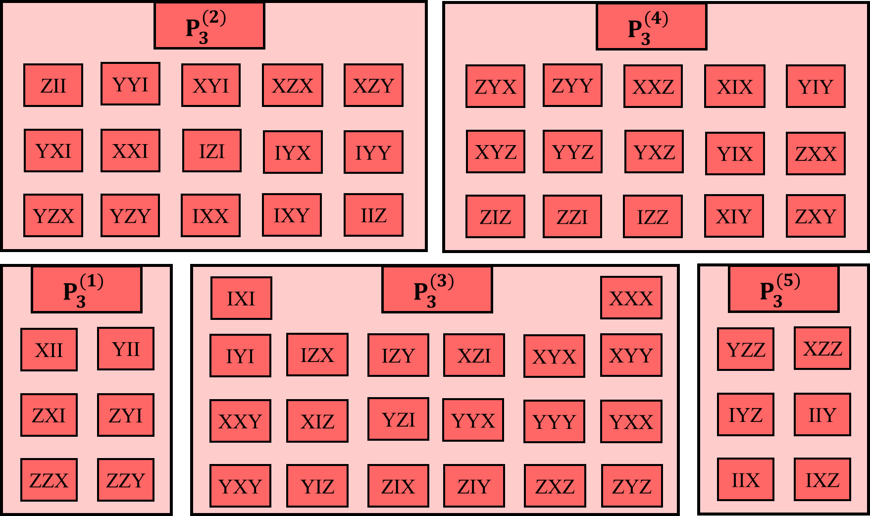
Figure 1: Subsets of $P_{3}$. There are 5 subsets, denoted as $P_{3}^{(k)}$ each of size $6\choose{k}$. $P_{3}^{(0)}=III$ and $P_{3}^{(6)}=ZZZ$, as well as factors of $i$ have been omitted for clarity.

We now consider the exact form of the linear operator $R$ in Equation 9 for the case of PI-SO matchgate simulation. For a generic universal circuit, one would expect $R:\mathcal{P}_{n}\rightarrow\mathcal{P}_{n}$ to be a $4^{n}-$dimensional orthogonal matrix. However, for a matchgate circuit, the corresponding linear operator, which we label $R_{MG}$, has a block diagonal structure where each block is an orthogonal matrix of size ${2n\choose k}$ acting on the span $\mathcal{P}^{(k)}_{n}$. In fact, each block is actually a compound matrix $\mathcal{R}^{(k)}_{2n}\in SO({2n\choose k})$ formed from the linear operator $R\in SO(2n)$ which arises in the proof of Theorem 1.

Definition 2

A compound matrix of order $k$ $\mathcal{R}^{(k)}_{2n}\in SO({2n\choose k})$, is a matrix formed a matrix $R\in SO(2n)$, such that $[\mathcal{R}^{(k)}_{2n}]_{ij}=det(R_{S_{i},S_{j}}),$ where $R_{S_{i},S_{j}}$ is a $k\times k$ minor of $R$, formed from rows given by the indices in the set $S_{i}=\{i_{1},\cdots,i_{k}\}$ and columns from $S_{j}=\{j_{1},\cdots,j_{k}\}.$

To see how compound matrices arise in the formulation of $R_{MG}$, let us consider the conjugation of an element of $\mathcal{L}^{(k)}_{n}$ by a Gaussian operation.

Theorem 2

Let $\mathcal{L}_{n}^{(k)}$ be the linear span of spinors of degree $k$. Let $U=e^{iH}$ be a Gaussian operation corresponding to a quadratic Hamiltonian H. Then conjugation of an element of $\mathcal{L}_{n}^{(k)}$ by $U$ is realized by a linear map $\mathcal{R}^{(k)}_{2n}$: $\mathcal{L}_{n}^{(k)}\rightarrow\mathcal{L}_{n}^{(k)}$.

Proof 2

Let $c_{\alpha_{1}}\cdots c_{\alpha_{k}}\in L_{n}^{(k)}$, where $\alpha_{1}<...<\alpha_{k}$. Then:

$$U^{\dagger}c_{\alpha_{1}}\cdots c_{\alpha_{k}}U=\sum_{\beta_{1},\cdots,\beta_{k}}^{2n}R_{\alpha_{1},\beta_{1}}\cdots R_{\alpha_{k},\beta_{k}}c_{\beta_{1}}\cdots c_{\beta_{k}},$$

where the identity $UU^{\dagger}$ has been inserted between each spinor, and Theorem 1 has been applied. No two values of indices $\beta_{i}$ or $\beta_{j}$ can be the same. This is because the sum over two different orthogonal columns of R is zero. The remaining terms with no repeated indices correspond to the k! permutations of the ${2n}\choose{k}$ combinations of the index set $\beta_{1},\cdots,\beta_{k}$. Each permutation is equivalent up to a sign depending on the ordering. Reordering the indices for each permutation, and collecting all like terms simplifies the expression to the following form:

$$U^{\dagger}c_{\alpha_{1}}\cdots c_{\alpha_{k}}U=\sum_{\beta_{1}<\cdots<\beta_{k}}^{2n}det(R^{\alpha_{1}\cdots\alpha_{k}}_{\beta_{1},\cdots,\beta_{k}})c_{\beta_{1}}\cdots c_{\beta_{k}},$$

where each coefficient is given by the determinant of a k $\times$ k minor of R, where the rows are selected by the values $\alpha_{1}\cdots\alpha_{k}$, and columns chosen by the values $\beta_{1},\cdots,\beta_{k}$. Each coefficient is an entry of the $kth$ order compound matrix $\mathcal{R}_{2n}^{(k)}$, acting on $\mathcal{L}_{n}^{(k)}$.

As each linear span $\mathcal{L}_{n}^{(k)}$ is mapped to itself under conjugation, this implies that the overall operation $R_{MG}:\mathcal{L}_{n}\rightarrow\mathcal{L}_{n}$ must be a block diagonal operator, where each block is given by $\mathcal{R}^{(k)}_{2n}$. We note that given the map between $\mathcal{L}_{n}$ and $P_{n}$ these results apply straightforwardly to the Pauli-basis.

1.4 Pauli-basis simulation of PI-SO matchgate circuits

Using the block diagonal structure of $R_{MG}$, we can see that PI-SO matchgate computation in the Pauli-Basis can be performed efficiently. Consider the computation:

$$\langle Z_{j}\rangle=\langle\langle Z_{j}|R_{MG}|\rho_{0}\rangle\rangle,$$ (10)

Here, $Z_{j}$ corresponds to a $Z$ measurement on qubit $j$, and $\rho_{0}$ is a product state where $\chi(\rho_{0})$ can be up to $4^{n}$. At first glance, the rank of $\rho_{0}$ suggests that evluating equation 10 via right-multiplication of $R_{MG}|\rho_{0}\rangle\rangle$ would be inefficient. However, given that in the single-mode output regime we are restricted to measurement operators which start in a bounded space: ie. $Z_{j}\in\mathcal{P}_{n}^{(2)}$ - by Theorem 2, we expect the vector $\langle\langle Z^{{}^{\prime}}_{j}|=\langle\langle Z_{j}|R_{MG}\in\mathcal{P}_{n}^{(2)}$ also. Given this, an efficient approach to evaluate the overall expression is to left multiply $R_{MG}$ with the measurement vector, which we refer to as a ‘Heisenberg’ approach. As the dynamics take place in the span $\mathcal{P}_{n}^{(2)}$, which is of size $\chi={2n\choose 2}$, we can construct the compound matrix $\mathcal{R}^{(2)}_{n}$ from $R\in SO(2n)$ which has $\mathcal{O}(\chi^{2})$ elements, and perform matrix-vector multiplication in one step with cost $\mathcal{O}(\chi^{2})$. While this approach is straightforward, it is possible to reduce this cost to $\mathcal{O}(N\chi)$, if we consider each gate seperately. That is, $R_{MG}=\prod_{i}R^{(i)}$. As each $R^{(i)}$ is constructed from a two-qubit gate, it will consist of $\frac{4^{n}}{16}$ tiles of a matrix $O\in SO(16)$ which corresponds to the rotation of the 16 two-qubit Pauli basis elements. Table 1 shows that for matchgates, $O$ will further be broken down into sub-matrices of sizes 1,4,6,4, and 1. Hence the compound matrix $[\mathcal{R}^{(i)}]^{(2)}_{n}$ will have a sparsity of at most s = 6. Given this, $[\mathcal{R}^{(i)}]^{(2)}_{n}$ can be implemented as $\approx\frac{\chi}{s}$ s-dimensional matrix-vector multiplications with cost $\mathcal{O}(s^{2})$. This which implies the overall cost of the computation across the N applications of $R^{(i)}$ is $\sim\mathcal{O}(N\chi s)$.

We finally note that the evaluation of the inner product $\langle\langle Z^{{}^{\prime}}_{k}|\rho_{0}\rangle\rangle$ has a cost $\sim\mathcal{O}(\chi)$, because only coefficients for basis terms present in both $|\rho_{0}\rangle\rangle$ and $\langle\langle Z^{{}^{\prime}}_{k}|$ contribute to the sum, for which there are at most $\chi$ such terms. Each relevant coefficient of $|\rho_{0}\rangle\rangle$ can be calculated via $\Tr(P_{i}\rho_{0})$, where $P_{i}\in\mathcal{P}_{n}^{(2)}$, which is efficient if $\rho_{0}$ is a product state.

2 Extension to non-matchgates

We now extend the Pauli-basis simulation method to include non-matchgates. To do this, we consider how non-matchgates transform elements of a linear span $\mathcal{L}_{n}^{(k)}$ and deduce the structure of the corresponding linear operator $R:$ $\mathcal{L}_{n}\rightarrow\mathcal{L}_{n}$. Specifically, we analyse the transformations induced by non-Gaussian operations, that is, those generated by elements of $L_{n}^{(d)}$ with $d\neq 2$. What we find is that the application of such an operation induces transformations across multiple linear spans, causing the space in which the dynamics take place, if initially bounded as in the PI-SO setting, to grow deterministically. To relate non-Gaussian operations to quantum computation, we show that any gate $U^{(1)}\in U(2)$ and $U^{(2)}\in U(4)$ can be reduced to two specific types of non-Gaussian operation, namely, those generated by quartic and odd-degree elements of $L_{n}$ respectively. Hence, we see it is possible to characterise the transformation induced by any gate of practical relevance.

2.1 Transformations induced by non-Gaussian operations

Let us consider the transformation of a basis element $c_{\{k\}}\in L_{n}^{(k)}$, under the operation $V^{\dagger}c_{\{k\}}V$, where $V$ is a non-Gaussian unitary of the form $e^{i\frac{\theta}{2}c_{\{d\}}}$, and $c_{\{d\}}\in L_{n}^{(d)}$. We further constrain $\theta\neq j\pi$ for $j\in\mathbb{Z}$ to guarantee non-trivial behaviour. Now, we have:

$$\begin{split}V^{\dagger}c_{\{k\}}V=&\cos^{2}{(\frac{\theta}{2})}c_{\{k\}}+\sin^{2}{(\frac{\theta}{2})}c_{\{d\}}c_{\{k\}}c_{\{d\}}+\\ &i\sin(\frac{\theta}{2})\cos(\frac{\theta}{2})(c_{\{d\}}c_{\{k\}}-c_{\{k\}}c_{\{d\}}),\\ \end{split}$$ (11)

where it can be seen that the expression simplifies depending on whether the monomials $c_{\{d\}}$ and $c_{\{k\}}$ commute or anti-commute. Indeed, this depends on the number of minus signs induced by rearranging $c_{\{d\}}c_{\{k\}}\rightarrow c_{\{k\}}c_{\{d\}}$, which is intimately related to the values d, k and a quantity $l\in[0,\textrm{min}(k,d)]$, which we define as $l=|\{k\}\cap\{d\}|$ (i.e. the number of spinors which occur in both $c_{\{d\}}$ and $c_{\{k\}}$):

Lemma 3

Let $k$ and $d$ be the degrees of $c_{\{k\}}$ and $c_{\{d\}}$ respectively. Let $l=|\{k\}\cap\{d\}|$ be the number of spinor indices common to both. Then $c_{\{d\}}c_{\{k\}}$ = $(-1)^{dk-l}c_{\{k\}}c_{\{d\}}$.

Proof 3

Majorana spinors anti-commute under permutation. This induces a sign depending on the number of permutations needed to transform $c_{\{k\}}c_{\{d\}}\rightarrow c_{\{d\}}c_{\{k\}}$. In the case l = 0 (no common spinors), the sign after this transform is $(-1)^{dk}$, as every spinor in $c_{\{k\}}$ is permuted past every spinor in $c_{\{d\}}$. When l is non-zero, l permutations will induce no sign (as these spinors will commute). Hence the overall sign induced after the full permutation is $(-1)^{dk-l}$.

We can discern that in the commuting case ($dk-l$ is even), the transformation simplifies to the identity channel. However, in the anti-commuting case ($dk-l$ is odd), the following rotation occurs:

$$V^{\dagger}c_{\{k\}}V=\cos(\theta)c_{\{k\}}+i\sin(\theta)c_{\{d\}}c_{\{k\}},$$ (12)

From equations 12 and 12, we see that non-matchgates transform $c_{\{k\}}$ to a space spanned by both $c_{\{k\}}$ and a monomial of the form $c_{\{d\}}c_{\{k\}}$. For a given value of $l$, $c_{\{d\}}c_{\{k\}}$ will simplify to $c_{\{d+k-2l\}}$, as two spinors with the same index will square to the identity. With these results, we can specify the linear span of the transformed monomial $V^{\dagger}c_{\{k\}}V$ as follows, depending on the values of $d$, $k$ and $l$:

$l$ parity	$kd$ odd	$kd$ even
$l\ even$	$\mathcal{L}_{n}^{(k)}\oplus\mathcal{L}_{n}^{(k+d-2l)}$	$\mathcal{L}_{n}^{(k)}$
$l\ odd$	$\mathcal{L}_{n}^{(k)}$	$\mathcal{L}_{n}^{(k)}\oplus\mathcal{L}_{n}^{(k+d-2l)}$

Table 2: Lookup table for the linear span to which $c_{\{k\}}\in L_{n}^{(k)}$ is transformed by a non-Gaussian operator of degree $d$, depending on the parity of $l$.

For a given $d$, $L_{n}^{(k)}$ will be split into $l$ subsets, each of which will be transformed differently by a non-Gaussian operation $V$, according to Table 2. For an element of a linear span $\mathcal{L}_{n}^{(k)}$, which is a linear combination of basis elements $c_{\{k\}}\in L_{n}^{(k)}$, we can say an element of $\mathcal{L}_{n}^{(k)}$ is transformed to the direct sum of the resultant linear spans of each transformed subset. To illustrate this, let us consider non-Gaussian operations corresponding to single- and two-qubit gates.

2.2 One-qubit non-Gaussian operations

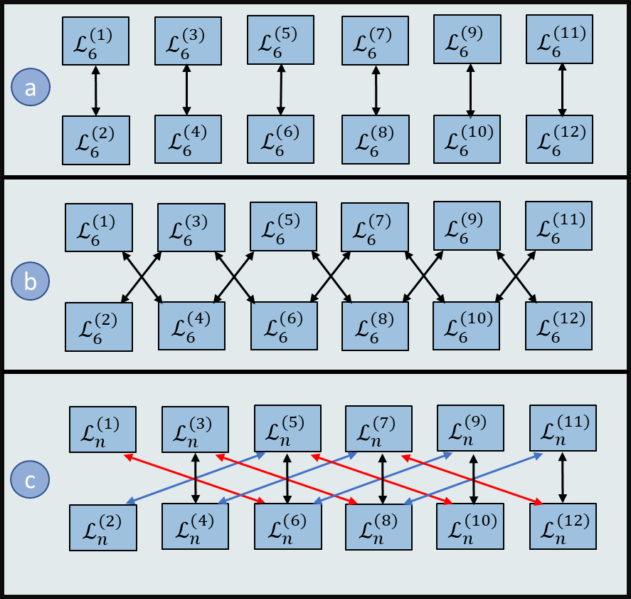
Figure 2: Transformation of an element of $\mathcal{L}_{6}^{(k)}$ under conjugation by an odd-degree non-Gaussian operation. Each arrow indicates the linear span to which a subset of $\mathcal{L}_{n}^{(k)}$ is transformed, corresponding to the possible values of $l$ for that basis set. (a) $d=1$, (b) $d=3$, (c) $d=5$ (Coloured arrows are for visualisation only).

Consider that any single-qubit gate can be decomposed, up to a global phase, as the product of three Euler rotations: $U^{(1)}=R_{z}(\theta_{1})R_{y}(\theta_{2})R_{z}(\theta_{3})$, parameterised by angles $\theta_{1},\theta_{2},\theta_{3}$. The $R_{z}(\theta)$ rotations in this decomposition can be expressed as matchgates, because $G(R_{z}(\theta),R_{z}(\theta))=R_{z}(\theta)\otimes\mathds{1}$, which implies that the non-Gaussian component of a single-qubit rotation is contained in $R_{y}(\theta)$. We can say that single-qubit gates $U^{(1)}$ are matchgate equivalent to $R_{y}$ gates.

An $R_{y}$ rotation applied to qubit $j$ can be expressed as $\cos(\frac{\theta}{2})I-i\sin(\frac{\theta}{2})Y_{j}$, where $Y_{j}=(-i)^{j-1}\prod_{i}^{j-1}({c_{2i-1}c_{2i}})c_{2j}$. It can be seen that the $R_{y}$ rotation is generated by odd-degree fermionic operators. Consider the simplest case where $j=1$, which corresponds to a non-Gaussian operation of degree $d=1$. The transformation induced on an element of $\mathcal{L}_{n}^{(k)}$ is given the following Theorem:

Theorem 4

Let $V=e^{i\theta c_{\{1\}}}$ be a degree 1 non-Gaussian operation. Then conjugation of an element of $\mathcal{L}_{n}^{(k)}$ by V is realized by a linear map $R_{V}^{(k)}$:

• For $k\ odd$:
  $R_{V}^{(k)}:$ $\mathcal{L}_{n}^{(k)}\oplus\mathcal{L}_{n}^{(k+1)}\rightarrow\mathcal{L}_{n}^{(k)}\oplus\mathcal{L}_{n}^{(k+1)}$

• For $k\ even$:
  $R_{V}^{(k)}:$ $\mathcal{L}_{n}^{(k)}\oplus\mathcal{L}_{n}^{(k-1)}\rightarrow\mathcal{L}_{n}^{(k)}\oplus\mathcal{L}_{n}^{(k-1)}$

Proof 4

For $d=1$, the possible values of $l$ are 0 and 1. This implies each set $L_{n}^{(k)}$ is composed of two subsets, each of which is transformed according to Table 2. Specifically, for $d=1$,

d = 1	k odd	k even
$l=0$	$\mathcal{L}_{n}^{(k)}\oplus\mathcal{L}_{n}^{(k+1)}$	$\mathcal{L}_{n}^{(k)}$
$l=1$	$\mathcal{L}_{n}^{(k)}$	$\mathcal{L}_{n}^{(k)}\oplus\mathcal{L}_{n}^{(k-1)}$

When k is odd, it can be seen that for each value of $l$, an element of $\mathcal{L}_{n}^{(k)}$ is transformed to the linear span $\mathcal{L}^{(k)}\oplus\mathcal{L}_{n}^{(k+1)}$. Similarly, when k is even, an element of $\mathcal{L}_{n}^{(k)}$ is transformed to the linear span $\mathcal{L}_{n}^{(k)}\oplus\mathcal{L}^{(k-1)}_{n}$.

The structure of the linear operator $R_{V}:\mathcal{L}_{n}\rightarrow\mathcal{L}_{n}$, with the transformation due to each $R_{V}^{(k)}$ is shown graphically in figure 2a. Here each arrow represents the transformation of a subset of $L_{n}^{(k)}$ corresponding to a particular value of $l$ (where a subset is transformed to its own linear span, no arrow is shown). It can be seen that under conjugation by an such an degree one non-gaussian operator (which is matchgate-equivalent to a single-qubit gate on the first qubit), Theorem 4 corroborates a result in [11] which states that matchgates plus arbitrary single-qubit gates on the first qubit are efficiently classically simulable in the PI-SO setting. This can be seen by the fact that the linear span in which the dynamics takes place, in this case, will be in $\mathcal{L}_{n}^{(1)}\oplus\mathcal{L}_{n}^{(2)}$, as single-qubits gates will, under conjugation, induce transformations in the space $\mathcal{L}_{n}^{(1)}\oplus\mathcal{L}_{n}^{(2)}$, and matchgates will induce transformations within the linear spans $\mathcal{L}_{n}^{(1)}$ and $\mathcal{L}_{n}^{(2)}$ separately due to Theorem 2.

For odd-degree non-Gaussian operations corresponding to single qubit gates on higher indexed qubits, the transformations induced become more complicated, as shown in Figure 2b ($d=3$) and Figure 2c ($d=5$). In these cases, efficient classical simulation is no longer possible as applying multiple single qubit gates interspersed with matchgates will in general induce transformation in the direct sum of linear spans which encompass an exponentially scaling portion of $L_{n}$.

2.3 Two-qubit non-Gaussian operations

To understand the transformations induced by two qubit gates, we make use of the fact that $U^{(2)}\in U(4)$ can be written (via a KAK decomposition [12][7]), in the following form:

$$\begin{aligned} U^{(2)}=\left(U_{1}\otimes U_{2}\right)e^{i(aX\otimes X+bY\otimes Y+cZ\otimes Z)}\left(U_{3}\otimes U_{4}\right)\end{aligned}.$$

Here the parameters $a$, $b$ and $c$ satisfy $a\geq b\geq c$ (to ensure the decomposition is unique.) Comparing this to the KAK decomposition for an arbitrary matchgate:

$$\left(e^{i\phi_{1}Z}\otimes e^{i\phi_{2}Z}\right)e^{i(aX\otimes X+bY\otimes Y)}\left(e^{i\phi_{3}Z}\otimes e^{i\phi_{4}Z}\right)$$

it can be seen that apart from the single qubit gates applied before and after the non-local core (which are matchgate-equivalent to $R_{y}$ rotations), by elimination, the gate $U_{ZZ}(\theta)$ = $e^{i\theta ZZ}$ must also induce non-Gaussian dynamics. Indeed, $U_{ZZ}(\theta)$ is a two-qubit parity-preserving gate which has been identified as enabling universal quantum computation when combined by Gaussian operations in [13], and corresponds to the unitary evolution of a degree four product of Majorana spinors. Specifically, when acting on qubits $a$ and $b$ (not necessarily nearest neighbour), one has $e^{i\theta Z_{a}Z_{b}}=e^{i\theta c_{2a-1},c_{2a},c_{2b-1},c_{2b}}$. It induces the following transformation on elements of $\mathcal{L}^{(k)}_{n}$:

Theorem 5

Let $U_{ZZ}(\theta)=e^{i\theta Z_{a}Z_{b}}=e^{i\theta c_{2a-1}c_{2a}c_{2b-1}c_{2b}}$ be a non-Gaussian gate acting on qubits a,b. Then for $n\geq 3$, conjugation of an element of $\mathcal{L}_{n}^{(k)}$ by $U_{ZZ}$ is realized by a linear map $R_{ZZ}^{(k)}$:

• For $k\in[1,2]:\\ R_{ZZ}^{(k)}:\mathcal{L}^{(k)}_{n}\oplus\mathcal{L}^{(k+2)}_{n}\rightarrow\mathcal{L}^{(k)}_{n}\oplus\mathcal{L}^{(k+2)}_{n}$

• For $k\in[3,2n-2]:\\ R_{ZZ}^{(k)}:\mathcal{L}^{(k-2)}_{n}\oplus\mathcal{L}^{(k)}_{n}\oplus\mathcal{L}^{(k+2)}_{n}\rightarrow\\ \mathcal{L}^{(k-2)}_{n}\oplus\mathcal{L}^{(k)}_{n}\oplus\mathcal{L}^{(k+2)}_{n}$

• for $k\in[2n-1,2n]:\\ R_{ZZ}^{(k)}:\mathcal{L}^{(k)}\oplus\mathcal{L}^{(k-2)}_{n}\rightarrow\mathcal{L}^{(k)}\oplus\mathcal{L}^{(k-2)}_{n}$

Proof 5

For d = 4, the possible values of l are 0,1,2,3,4. Hence the set $L_{n}^{(k)}$ consists of five subsets for each value of l. Given the product 4k is always even, we need only consider the even column of Table 2, for which we enumerate the following transformations:

$d=4$	4k even
$l=0$	$\mathcal{L}_{n}^{(k)}$
$l=1$	$\mathcal{L}_{n}^{(k)}\oplus\mathcal{L}_{n}^{(k+2)}$
$l=2$	$\mathcal{L}_{n}^{(k)}$
$l=3$	$\mathcal{L}_{n}^{(k)}\oplus\mathcal{L}^{(k-2)}_{n}$
$l=4$	$\mathcal{L}_{n}^{(k)}$

For the first case where k = 1 or 2, $l$ is limited to be 0,1, or 2. For any of these values, $\mathcal{L}^{(k)}_{n}$ is transformed to the linear span $\mathcal{L}^{(k)}_{n}\oplus\mathcal{L}^{(k+2)}_{n}$. In the general case, ${L}^{(k)}_{n}$ is transformed to $\mathcal{L}^{(k-2)}\oplus\mathcal{L}_{n}^{(k)}\oplus\mathcal{L}_{n}^{(k+2)}$. For k = 2n-1, 2n-2: $l$ can be either l = 4, 3 or 2, which means $\mathcal{L}^{(k)}_{n}$ is transformed to $\mathcal{L}^{(k)}\oplus\mathcal{L}^{(k-2)}_{n}$.

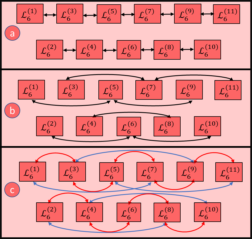
Figure 3: Transformation of an element of $\mathcal{L}_{6}^{(k)}$ under conjugation by an even-degree non-Gaussian operation. Each arrow indicates the linear span to which a subset of $\mathcal{L}_{n}^{(k)}$ is transformed, corresponding to the possible values of $l$ for that basis set. (a) $d=4$, (b) $d=6$, (c) $d=8$ (Coloured arrows are for visualisation only).

A schematic of the overall operation $R_{ZZ}:\mathcal{L}_{n}\rightarrow\mathcal{L}_{n}$ is shown in Figure 3a. The matrix $R_{ZZ}$ manifests as a signed permutation matrix mapping elements $p\in P_{n}$ to $ZZp$. There are many interesting two qubit gates which are matchgate equivalent to $U_{ZZ}(\theta)$, including SWAP, CZ, and CPhase, which all belong to a general family of gates called parity-preserving non-matchgates, introduced by Brod in [7]. These gates are of the form $G(A,B)$, but $det(A)\neq det(B)$. Theorem 4 implies that any (nearest-neighbour) parity preserving non-matchgate will transform across linear spans as shown in figure 3a. Once again, the transformations induced by higher degree non-Gaussian operations, specifically d = 6 and d = 8 are shown in Figure 3 for completeness. In general, these would correspond to three and four-qubit gates in the Jordan-Wigner mapping and hence are not of practical relevance.

In this section, we have shown how elements of linear spans $\mathcal{L}_{n}^{(k)}$, and hence $\mathcal{P}_{n}^{(k)}$, are transformed by the conjugation of an arbitrary non-Gaussian operation. Unlike Gaussian operations, which induce a transformation across a single span, $\mathcal{L}_{n}^{(k)}$, non-Gaussian operations induce linear maps across multiple spans. For PI-SO simulation, this suggests that it is possible to straightforwardly extend the Pauli-basis simulation method by expanding the Pauli-basis vector space, $\mathcal{P}_{n}^{(k)}$, to include newly accessed linear spans due to non-matchgates over the course of the dynamics. While this is possible with any non-matchgate by considering the relevant transformations in Figures 2 and 3 - in the following section, we focus on parity-preserving non-matchgates as they include gates which occur commonly in universal matchgate circuits.

3 Classical simulation of ‘matchgate + ZZ’ circuits

Let us denote an $n$-qubit matchgate circuit supplemented with $m$ parity-preserving non-matchgates as a ‘matchgate + ZZ’ circuit. Such a circuit can be generally written in the form $U=U^{(m)}_{MG}U^{(m)}_{ZZ}...U_{MG}^{(1)}U_{ZZ}^{(1)}U_{MG}^{(0)}$, where there are $m+1$ matchgate circuits interleaved with $m$ nearest neighbour $U_{ZZ}(\theta)$ gates, with N gates in total. We note that this form is general for any parity preserving non-matchgate as the matchgate component of these gates can be absorbed into the adjacent matchgate circuits. Furthermore, we impose no structure on the matchgate circuits themselves, which can be random, pyramidal or a brick wall structure [14]. We do however consider two variants of overall ‘matchgate + ZZ’ structure, which we refer to as random and layered. A random circuit refers to when the ZZ gates are placed randomly between the matchgate circuits. A layered circuit refers to when all ZZ gates are equally spaced.

From Theorem 5, we have seen that a $U_{ZZ}(\theta)$ gate induces a linear map in the Pauli basis, denoted $R_{ZZ}$, which in general acts transforms elements from $\mathcal{P}_{n}^{(k-2)}\oplus\mathcal{P}_{n}^{(k)}\oplus\mathcal{P}_{n}^{(k+2)}$ to $\mathcal{P}_{n}^{(k-2)}\oplus\mathcal{P}_{n}^{(k)}\oplus\mathcal{P}_{n}^{(k+2)}$. If $U_{ZZ}(\theta)$ gates are applied at different points in the circuit, further reaching linear spans will be accessed in a stepwise fashion. This suggests, starting from a measurement operator in $\mathcal{P}_{n}^{(2)}$, for example, it is possible to apply a small number (up to a maximum of $n-2$) of $U_{ZZ}(\theta)$ gates before the entire even fermionic algebra is accessed. In the next section, we show how a ‘matchgate + ZZ’ circuit can be simulated by applying this insight to the Pauli-basis method introduced in Section 1.4.

3.1 Sparse ’Matchgate + ZZ’ Simulation

The PI-SO simulation problem with respect to a ‘matchgate + ZZ’ circuit can be written, using equation 9 as:

$$\langle Z_{j}\rangle=\langle\langle Z_{j}|R_{MG}^{(m)}R_{ZZ}^{(m)}...R^{(1)}_{MG}R^{(1)}_{ZZ}R^{(0)}_{MG}|\rho_{0}\rangle\rangle,$$ (13)

where each matchgate circuit $R_{MG}=\prod_{k}R_{i,i+1}^{(k)}$ is a product of individual gates which act on qubits $i$ and $i+1$. Furthermore, each $R^{(m)}_{ZZ}$ is the linear operator corresponding to a $U_{ZZ}$ gate acting on arbitrary nearest neighbour qubits. To evaluate equation 13 efficiently, we use the ‘Heisenberg’ approach as used in Section 1.4. Furthermore, we use sparse data structures to ensure that no (initially) exponentially-sized object needs to be allocated to memory. Specifically, we can store $\langle\langle Z_{j}^{{}^{\prime}}|$ during the computation as a dictionary of keys: $\langle\langle Z_{j}^{{}^{\prime}}|=\{(P_{1}:v_{1}),\dots,(P_{\chi}:v_{\chi})\}$, where each key-value pair corresponds to a $n$-qubit Pauli operator and its coefficient in a Pauli-basis decomposition. Matrix-vector multiplication $\langle\langle Z_{j}^{{}^{\prime}}|R$ is then performed by (1), constructing a sparse representation of each constituent $R$ matrix (an individual $R_{i,i+1}^{(k)}$ or $R_{ZZ}$ matrix), (2) cycling through each key in $\langle\langle Z_{j}^{{}^{\prime}}|$ and determining which basis elements are rotated by $R$, and (3) updating the corresponding values with matrix-vector multiplication.

To do step (1) efficiently, we can again use the observation that each $R$ matrix is fully characterised by a rotation matrix $O\in SO(16)$ acting on a two-qubit subspace of Pauli operators, stemming from the fact that each gate is two-qubit. For each operator constituting $R_{MG}$, the structure of $O$ is a sparse block-diagonal with 1,4,6,4,1 dimensional submatrices corresponding to a rotation of the basis of $P_{2}^{(k)}$. The submatrices are calculated as shown in Subroutine 1. For $R_{ZZ}$, the corresponding $O$ matrix will be a signed permutation matrix mapping an element $p\in P_{2}$ to $ZZp$.

Subroutine 1: Rotations(U)
Input: $U$
Output: 1,4,6,4,1 dim matrices $R_{(0)},R_{(1)},R_{(2)},R_{(3)},R_{(4)}$
For $d\in[0,4]:$ For $p^{(d)}_{\alpha}$, $p^{(d)}_{\beta}$ in $P_{2}^{(d)}$: $[R_{(d)}]_{\alpha\beta}=\mathrm{Tr}(U^{\dagger}p_{\alpha}^{(d)}Up_{\beta}^{(d)})$

Subroutine 2: Find(P)
Input: A n-qubit Pauli operator $P$, qubit indices $j,j+1$
Output: Subset of $P_{2}$, $d$
              $\vec{P}=\{P_{1},...,P_{m}\}$ where $m=|P_{2}^{(d)}|$,
$\textit{support}\leftarrow P_{j,j+1}\in P_{2}^{(d)}$
$\textit{stem}\leftarrow P_{n-(j,j+1)}$
For $p^{(d)}\in P_{2}^{(d)}$:
          $P_{\alpha}=P_{n-(j,j+1)}\otimes p^{(d)}$

Subroutine 3: Update($\langle\langle M|,\vec{P},R^{i}_{(d)})$)
Input: A set of keys $\vec{P}$, DofK $\langle\langle M|$
Output: Updated DofK $\langle\langle M|$
For $P_{i}\in\vec{P}$:
          If $(P_{i},v_{i})\in\langle\langle M|$: $\vec{v}\leftarrow v_{i}$
          Else: $\vec{v}\leftarrow 0$
$\vec{v^{{}^{\prime}}}\leftarrow R_{(d)}\vec{v}$
$\langle\langle M|\leftarrow({\vec{P}},\vec{v})$

For step (2), we identify the elements of $\langle\langle Z_{j}^{{}^{\prime}}|$ which are rotated by each O matrix. To do this, we split every key into its support and a stem on qubits $j,j+1$ denoted $P_{j,j+1}$ and $P_{n-j,j+1}$ respectively, describing the support of the key on the qubits $j$ and $j+1$, and its complement. The rotation will be the same for all keys with the same support. Hence, if $P_{j,j+1}\in P_{2}^{(d)}$, then the new basis elements following rotation are obtained by the tensor product of elements of $P_{2}^{(d)}$ with the stem (Subroutine 2).

Algorithm 1: Sparse Pauli-basis simulation for ‘Matchgate+ZZ’ circuit
Inputs: Observable M, ’matchgate + ZZ’ circuit: $U=U^{(m)}_{MG}U^{(m)}_{ZZ}...U_{MG}^{(1)}U_{ZZ}^{(1)}U_{MG}^{(0)}$ on $n$ qubits, Initial product state $\rho_{0}$. Outputs: Expectation value $\langle M\rangle=Tr(U^{\dagger}MU\rho_{0})$ Procedure:
Initialise measurement vector (e.g. $\langle\langle M|$ ${\leftarrow(Z_{k}:1.0)}$) as dictionary of keys. Matrix-vector Multiplication For gates $U^{(i)}_{j,j+1}\in U_{MG}$ acting on qubits j, j+1:
         $R^{(i)}_{(0)},R^{(i)}_{(1)},R^{(i)}_{(2)},R^{(i)}_{(3)},R^{(i)}_{(4)}\leftarrow\textbf{Rotations}(U^{(i)}_{j,j+1})$
           $\textit{temp}\leftarrow\{\}$
          For    $(P^{(m)},v^{(m)})\in\langle\langle M|$:
                  If $P^{(m)}\notin\textit{temp}$:
                           $\vec{P},d\leftarrow$ Find($P^{(m)}$)
                           $\langle\langle M|\leftarrow\textbf{Update}(\langle\langle M|,\vec{P},R^{(i)}_{(d)})$
                          $\textit{temp}\leftarrow\vec{P}$ Inner Product
For $(P_{n}^{(m)},v_{m})\in\langle\langle M|$:           $\langle{M}\rangle\mathrel{+}=Tr(\rho_{0}P_{n}^{(m)})v_{m}$

As an example, consider a rotation supported on qubits 1 and 2. Then a key $ZIXY$ is split into $ZI$ (support) and $XY$ (stem). As the support is in $P_{2}^{(2)}$, the basis elements accessed in a rotation will be $ZIXY,IZXY,XXXY,YYXY,XYXY,YXXY$. We can store dictionary keys as integers by encoding $n$-qubit Pauli operator as a bitstring of size $2n$, where $I=00$, $X=01$, $Y=10$, and $Z=11$. Find(P) can then be efficiently implemented as integer addition and subtraction. Finally, we perform an update of the identified key-value pairs by performing a matrix-vector multiplication between the multiplication of the coefficients $\vec{v}$ corresponding to $\vec{P}$ (Subroutine 3).

The overall matrix-vector multiplication uses these three subroutines as shown in Algorithm 1. As the measurement vector is constantly being updated, it is important to keep track of which keys have already been rotated to avoid redundant multiplication. For this purpose, a separate data structure with $\mathcal{O}$(1) write/read cost, labelled temp (such as a hash table) is used to store the keys already accessed using ‘Find’.

The total simulation cost is proportional to a quantity denoted $\chi_{t}=\sum_{i}\chi_{i}$ which is the total sum of the Pauli ranks at each step of the circuit. The relevance of $\chi_{t}$ follows from the fact that the various contributions to the time cost are characterised by $\chi_{i}=\chi(Z_{j}^{{}^{\prime}})$ at each iteration. Specifically, the number of ‘Find’ and ‘Update’ calls for each gate can be approximated by $\frac{\chi_{i}}{s}$, where $s$ is the maximum sparsity of each R matrix (which for $R_{MG}$ is s = 6, and $R_{ZZ}$ is s=1). Whereas ‘Find’ can be implemented as integer addition (which is efficient), matrix-vector multiplications during ‘Update’ calls will cost $\sim$ $\mathcal{O}(s^{2})$. Hence the dominant time cost for a single matrix-vector multiplication will be $\mathcal{O}(\frac{\chi_{i}}{s}s^{2})=\mathcal{O}(\chi_{i}s)$. Summing the costs across the entire circuit, the overall time cost will be $\mathcal{O}(\chi_{t}s)$. Hence, determining the overall time complexity of the algorithm reduces to finding suitable bounds for $\chi_{t}$, which is the subject of the next section.

3.2 Heuristic Improvements

We now introduce two methods to improve the proposed simulation method. The first improvement is to use what is sometimes known as an interaction picture approach, which describes applying R operators to both $|\rho_{0}\rangle\rangle$ and $\langle\langle Z_{j}|$. This reduces the number of iterations with a large number of multiplications which often occur in the final gates of a layered circuit. It also introduces parallelism as the two directions of multiplication can be computed independently. To initialise $|\rho_{0}\rangle\rangle$ using this method, one need only consider elements in the linear spans which will be accessed following the application of $m$ parity-preserving non-matchgates gates. For computational zero states, this will be Pauli operators containing up to $m$ $Z$ operators.

The second method is to apply pruning, where coefficients from $\langle\langle M|$ which are below some threshold value $\epsilon$ are removed before the application of the next operator. At the cost of some error in the final expectation value, this heuristic has the potential to greatly reduce the time cost for certain circuits. This method is shown in practice in the final section.

3.3 Pauli rank profile for ‘matchgate + ZZ’ circuit

To bound $\chi_{t}$, it is instructive to plot $\chi(Z_{j}^{{}^{\prime}})$, as a function of the gate index. We refer to this as the ‘Pauli rank profile’ of a circuit. In this context, we can intuit $\chi_{t}$ to be the area ‘under the curve’ of such a profile. In what follows, we plot the Pauli profile for four different types of circuits, which all have differences in scaling in the limit of large $n$. We first consider random circuits, where ZZ gates are placed randomly throughout the circuit. In this case, the simulation cost can vary a lot depending on the exact positions of the ZZ gates. In the the worst-case scenario, the ZZ gates are placed late in the circuit (and hence left-multiplied early on). This is shown in Figure 4a. In this case, we can loosely approximate $\chi_{t}\approx N\chi_{max}$, where $N\chi_{max}$ is given by the sum of the size of each linear span accessed when $m$ ZZ gates are applied. Let us denote $N\chi_{max}$ as $\chi_{t}^{(general)}$, as this bound applies generally to any circuit. Then, analytically:

$$\chi_{t}(n,m)\approx \chi^{(general)}_{t}$$ (14)

$$=N\sum_{s=1}^{m}|L^{(2m+4-2s)}_{n}|$$

$$=N\sum_{s=1}^{m}{2n\choose 2m+4-2s},$$

which is a partial sum of even binomial coefficients corresponding to the sizes of each accessed linear span. We make an important observation that when $m$ is less than a critical value denoted $m_{c}=\lfloor\frac{n}{2}\rfloor-1$, to be proved in the next section, the scaling is qualitatively different [see 4b]. In fact, in this regime, the scaling is polynomial in $n$. Whereas, in the regime where $m>m_{c}$, the scaling is exponential. The second type of circuit we consider is a layered circuit. In this case, we assume that ZZ gates are equally spaced. This represents an average simulation hardness, and it is possible to make tighter guarantees on the simulation costs given its regular structure. We can approximate $\chi_{t}$ in this case by adding the size of each horizontal step, whose height is given by $|L_{n}^{(k)}|$ and whose width is an integer multiple of $\frac{N}{m+1}$. In this case the quantity $\chi_{t}$ is well approximated as:

$$\chi_{t}(n,m)\approx \chi_{t}^{(layered)}$$ (15)

$$=\frac{N}{m+1}\sum_{s=1}^{m}s|L^{(2m+4-2s)}_{n}|$$

$$=\frac{N}{m+1}\sum_{s=1}^{m}s{2n\choose{2m+4-2s}}.$$

Once again, we make a distinction between the regime where $m<m_{c}$ and $m\geq m_{c}$, which have qualitatively different pauli rank profiles shown in Figures 4c and 4d. As a final note, we also plot the Pauli rank profile of an interaction approach to matrix-vector multiplication in blue, where the right portion of the diagram represents $\chi(\rho_{0})$. While for the regime $m\geq m_{c}$, the reduction in time cost is negligible, it is possible to save an appreciable amount when $m<m_{c}$ for the high-rank multiplications which take place towards the end of the computation

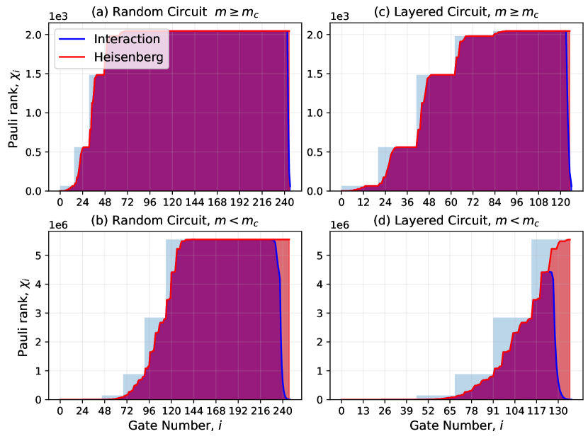
Figure 4: Pauli rank profile for four types of circuit. All circuit contain four ZZ gates, with interspersing matchgate circuits having brickwall structure, but for m > m_c we consider 6 qubits, whereas for $m<m_{c}$ we consider 12. The structures for each are very different, and hence have different asymptotic scaling in the limit of large $n$.

4 Bounds on simulation time costs

The approximations $\chi_{t}^{(general)}$ and $\chi_{t}^{(layered)}$ are given in exact terms above. However, it is known that the partial sum of binomial coefficients has no closed-form expression and must be bounded. In Figure 5, we plot $\frac{\chi_{t}^{(general)}}{N}$ as a function of $m$ (black line), for different values of $n$. We also plot its bound that we derive in this section (blue dashed line). We notice that there is a critical point at $m=m_{c}=\lfloor\frac{n}{2}\rfloor-1$, where the scaling in $n$ qualitatively changes from polynomial to exponential in nature. In deriving the bounds, we consider each regime separately.

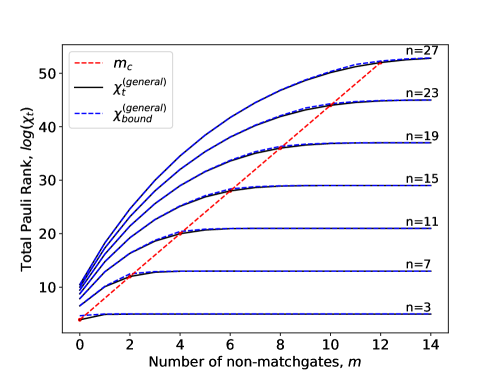
Figure 5: A plot of $\chi_{t}^{(general)}$ (red) and $\chi_{t}^{(bound)}$ (blue) versus $m$. It can be seen that there is a transition between polynomial scaling and exponential scaling at a critical point $m_{c}=\lfloor\frac{n}{2}\rfloor-1$.

4.1 Bounds for polynomial regime

To bound $\chi_{t}^{(general)}$ and $\chi_{t}^{(layered)}$ When $m<m_{c}$, we use the following result for bound of the partial sum of binomial coefficients when m is fixed.

Lemma 6

The following relations hold:

$$\sum_{s=1}^{m}{2n\choose{2m+4-2s}}<{2n\choose{2m+2}}\frac{1}{1-r}$$ (16)

$$\sum_{s=1}^{m}s{2n\choose{2m+4-2s}}<{2n\choose{2m+2}}\frac{1}{(1-r)^{2}}$$ (17)

where $r=(\frac{2m+2}{2n-2m-1})^{2}$, and $m\leq\lfloor\frac{n}{2}\rfloor-1$

Proof 6

Consider that:

$$\frac{{p\choose{k}}+{p\choose{k-2}}+...}{{p\choose{k}}}=1+\frac{k(k-1)}{(p-k+1)(p-k+2)}+...,$$ (18)

We notice that we can bound this above by:

$$1+(\frac{k}{p-k+1})^{2}+...,$$ (19)

which is an infinite geometric series with ratio $r=(\frac{k}{p-k+1})^{2}$. This series converges to $\frac{1}{1-r}$, for $0\leq r<1$. Using the substitution that $p=2n$ and $k=2m+2$, $r=(\frac{2m+2}{2n-2m-1})^{2}$ and the series converges as long as $0\leq m\leq\lfloor\frac{n}{2}\rfloor-1$. To prove inequality 17, we can use the result that $\sum_{k=1}^{\infty}kr^{k}=\frac{r}{(1-r)^{2}}$. If we correspondingly modify equation 19 with integer weights:

$$1+2(\frac{k}{p-k+1})^{2}+...,$$ (20)

we notice this is is equal to $\sum_{k=1}^{\infty}kr^{k-1}=\frac{1}{(1-r)^{2}}$

We now combine these results in Theorem 7 to give a closed-form expression for bounds of $\chi_{t}^{(general)}$ and $\chi_{t}^{(layered)}$.

Theorem 7

For $m\leq m_{c}=\lfloor\frac{n}{2}\rfloor-1$:

$$\chi_{bound}^{(general)}(n,m)<N{2n\choose{2m+2}}\frac{1}{(1-r)},$$ (21)

$$\chi_{bound}^{(layered)}(n,m)<\frac{N}{m+1}{2n\choose{2m+2}}\frac{1}{(1-r)^{2}},$$ (22)

for $r=(\frac{2m+2}{2n-2m-1})^{2}$ and $m\leq m_{c}=\lfloor\frac{n}{2}\rfloor-1$.

Proof 7

The expression for $\chi_{bound}^{(general)}$ and $\chi_{bound}^{(layered)}$ follow directly from Equation 16 and 17.

For each bound, we can consider the asymptotic scaling as $n\rightarrow\infty$ with fixed $m$. We can see that in this limit, $r\rightarrow 0$, and the scaling is dominated by ${2n\choose{2m+2}}$. Hence we can conclude the following two results, using the relation that ${2n\choose{2m+2}}<\frac{ne}{m+1}^{2m+2}$, where e is Eulers constant:

Corollary 1

For fixed $m<m_{c}$, as $n\rightarrow\infty$, $\chi_{bound}^{(general)}$ scales as $\mathcal{O}(N(\frac{ne}{m+1})^{2m+2})$.

Corollary 2

For fixed $m<m_{c}$, as $n\rightarrow\infty$, $\chi_{bound}^{(layered)}$ scales as $\mathcal{O}(\frac{N}{m+1}(\frac{ne}{m+1})^{2m+2}).$

This implies the total simulation cost of the algorithm, which is on the order of $\sim\mathcal{O}(\chi_{t}s)$ will in the worst case scale polynomially in $n$, for fixed $m<m_{c}$.

4.2 Bounds for exponential regime

For the regime where $m\geq m_{c}$, we know that the asymptotic scaling for both $\chi_{bound}^{(general)}$ and $\chi_{bound}^{(layered)}$ will be exponential. In the first case, we can see that when $m_{c}<m\leq n-2$ the value of $\chi_{max}$ will range between $2^{2n-2}$ and $2^{2n-1}$. This implies that $\chi_{bound}^{(general)}$ will vary between $N2^{2n-2}$ and $N2^{2n-1}$. In the appendix, we interpolate this regime by approximating the value of $\chi_{max}$ with the cumulative distribution function, $\Phi(\alpha)$ of the normal approximation to binomial distribution containing only even coefficients. This gives a bound of:

$$\chi^{(general)}_{bound}(n,m)=N2^{2n-1}\Phi(\sqrt{\frac{8}{n}}(m-m_{c}+0.5)),$$ (23)

which is plotted for the region $m\geq m_{c}$ in Figure 5. We have $\frac{1}{2}<\Phi(\alpha)\leq 1$, and $\Phi(1)=0.84$, which implies that for $m>\frac{n}{\sqrt{8}}-1+m_{c}$ adding further parity-preserving non-matchgates has small constant factor effects on the scaling. For the general bound, we can conclude:

Corollary 3

For $m_{c}<m<n-2$, as $n\rightarrow\infty$, $\chi_{bound}^{(general)}$ scales as $\sim\mathcal{O}(N2^{2n-1-log_{2}(\Phi(\alpha))})$, where $\alpha=\sqrt{\frac{8}{n}}(m-m_{c}+0.5)$.

For the case of $\chi_{bound}^{(layered)}$, we can also argue that when $m_{c}<m\leq n-2$: the asymptotic scaling of $\chi_{t}$ will vary between $\sim\mathcal{O}(\frac{N}{n+1}\frac{4^{n}}{\sqrt{\pi n}})$ and $\sim\mathcal{O}(N\frac{4^{n}}{\sqrt{\pi n}})$, which is shown in the appendix. Hence, for both cases, compared to the scaling of a dense state vector simulator which scales as $\mathcal{O}(N4^{n})$ for a circuit containing N gates, this method will always outperform such a simulator in the asymptotic limit.

5 Fermi-Hubbard Model Simulation using Pauli-basis Simulation

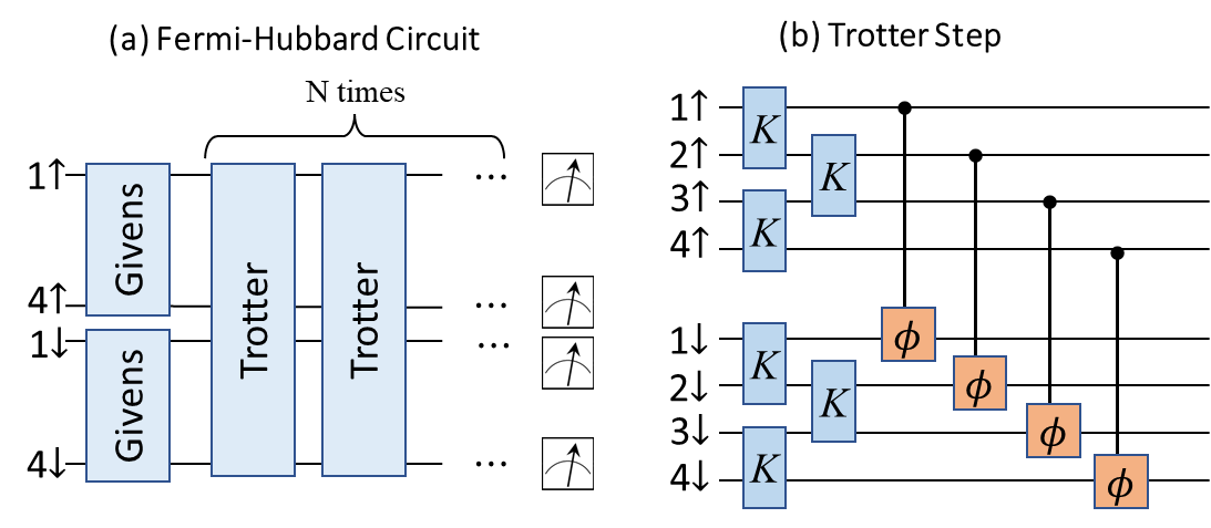
Figure 6: Circuit used to simulate time evolution of $H_{FH}$ given in Equation 24, from [1]. (a) Overall circuit, consisting of initialisation of Hartree-Fock state using Given’s rotations, which are treated as black box matchgate circuits. This is followed by $m$ Trotter steps and finally, measurement (b) Trotter step, consisting of odd-even hopping gates, even-odd hopping gates (blue) and onsite interactions (orange). In the interaction-limited case, only a finite number of cPhase gates connect the top and bottom registers.

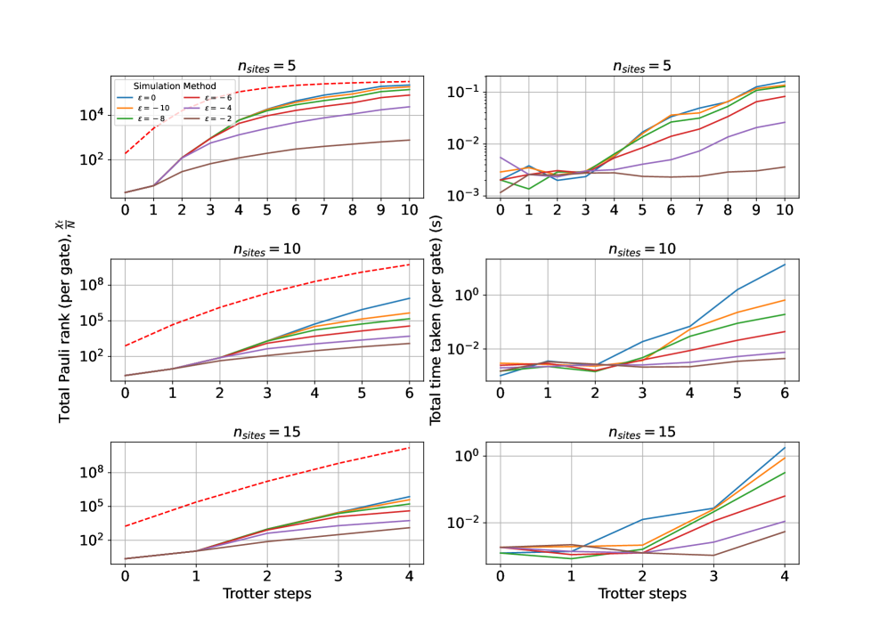
Figure 7: Total Pauli rank/Time (per gate) required to evaluate $\langle Z_{j}\rangle$ as a function of the number of Trotter Steps of an interaction limited version of the circuit shown in Figure 6. The red dashed line indicates the value of $\chi_{t}^{(layered}$ for layered circuits derived in Section 5. For simulations with a pruning threshold, we can greatly reduce the simulation cost, however, we incur an error $\delta$ which varies as shown in Figure 8.

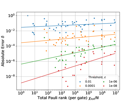
Figure 8: Absolute Error of expectation value for different values of pruning threshold, as a function of the total Pauli rank, $\chi_{tot}$ of a simulation. Each point corresponds to a Trotter circuit simulated with different values of $n$ and $T$. The same set of circuits is used for each threshold value, and where the absolute error was zero, no point is shown.

The method is now demonstrated in the restricted setting of an interaction-limited 1D Fermi-Hubbard model. The Fermi-Hubbard model is a widely used model in condensed matter physics to understand the properties of correlated fermionic systems. A 1D model consists of $p$ sites, arranged in a line, with $q<2p$ fermions distributed between these sites. Each site can contain a spin-up fermion, a spin-down fermion or both. Fermions can hop between adjacent sites, characterised by an energy $J$, and interact with a coulombic repulsion each other if a site is doubly occupied, characterised by an energy $U$. The Hamiltonian of the system is given below:

$$H_{FH}= -J\sum_{j=1}^{L-1}\sum_{\nu=\uparrow,\downarrow}c_{j,\nu}^{\dagger}c_{j+1,\nu}+\text{ h.c. }$$ (24)

$$+U\sum_{j=1}^{L}n_{j,\uparrow}n_{j,\downarrow},$$

where the first term corresponds to hopping and the second term to the onsite interaction terms respectively. In this model, the presence of the interaction term leads to interesting, but difficult-to-simulate behaviour. Simulating this Hamiltonian can be achieved using the Lie product formula:

$$e^{i(H_{hop}+H_{int})t}=\lim_{N\to\infty}\{e^{iH_{hop}\frac{t}{N}}e^{iH_{int}\frac{t}{N}}\}^{N},$$

which approximates the dynamics induced by the total Hamiltonian as the product of the individual hopping and interacting unitary operators, applied for a fractional amount of time. In practice, the series is truncated to a particular number of steps known as the trotter number $T$. Each individual unitary can be decomposed as a circuit on $2n$ qubits, where the first and second register of $n$ qubits correspond to spin up and spin down electrons respectively. The circuit representing the overall computation and a single Trotter step is represented diagrammatically in Figure 1.

It can be seen that the circuit factorises into a familiar form: $U_{FH}=U^{(T)}_{MG}U^{(T)}_{\phi}\dots U_{MG}^{(1)}U_{\phi}^{(1)}U^{(0)}_{MG}$, where the superscript $i$ corresponds to the Trotter step index. The circuit is randomly initialised in the ground state of a non-interacting quadratic Hamiltonian. This can be implemented as a ladder of q parallel nearest-neighbour Given’s rotations which are matchgate circuits with roughly $\mathcal{O}(nq)$ gates, represented by the circuit $U^{(0)}_{MG}$. As the value of $q$ doesn’t impact the overall scaling, we choose the simplest case where $q$ = 1, which is a single ladder of Given’s rotations. Gates corresponding to onsite interactions denote non-nearest-neighbour CPhase gates. Indeed, CPhase gates are matchgate equivalent to $U_{ZZ}=e^{i\theta ZZ}$, specifically taking the form $\textrm{CPhase}(\theta)$ = $e^{i\theta ZZ}G(R_{z}(2\theta),I)$. The fact that c-Phase acts on distant qubits a and b poses no issue (in this case) as $R_{z}^{a}\otimes I$ and $I\otimes R_{z}^{b}$ be expressed as G($R_{z}(\theta),R_{z}(\theta)$)) G($R_{z}(\theta),R_{z}(-\theta)$) respectively, and the transformations induced by $e^{i\theta Z_{a}Z_{b}}$ hold for any qubits a and b, according to Theorem • ‣ 5.

To test Algorithm 1, we consider the simulation of Trotter circuits with limited interactions, where only a finite number of CPhase are present in each Trotter step. This corresponds to removing on-site interaction for particular sites in the Fermi-Hubbard model. This paradigm may be useful for error mitigation methods which use efficient simulation of ‘training circuits’ to understand and mitigate errors in a related universal circuit [15]. Typically, such training circuits would have to be from gate sets which are classically simulable but may not be functionally similar to the circuit being implemented. By extending the reach of classical simulation methods to universal circuits it is possible that such methods could perform better.

In Figure 7 we show the scaling of $\chi_{tot}$ (per gate) as a function of the number of Trotter steps, each step containing a single CPhase gate between the first qubit of the upper and lower register. In this case, the number of Trotter steps is equal to the number of parity-preserving non-matchgates. In our tests, we compare two methods that are specified by Algorithm 1, and a series of modified versions where a pruning threshold is set to $\epsilon$. We simulate using each method randomly initialised Givens circuits, consisting of $n_{sites}=5,10,15$ sites (corresponding n = 10, 20, 30 qubits respectively), for a number of Trotter steps $T$ in the range [0,10]. We further normalise the rank and time by the number of gates, the number of which is given by $N=2n_{sites}(T+1)$. From Figure 8, we verify our prediction that the simulator scales polynomially in the qubit number $n$, but exponentially in the number of parity-preserving non-matchgates. Furthermore, ignoring transient effects for small circuit depths, the time taken scales in proportion with the Pauli rank.

Pruning methods greatly increase the reach of Trotter circuit simulation at the cost of incurring a small error in the calculation of the final expectation value. The relationship between the incurred error $(\delta)$ and the total pruning-free ($\epsilon=0$) Pauli rank (per gate) is plotted in Figure 5. We consider the range of ranks accessed in our simulations, for different values of the pruning threshold $(\epsilon)$. Each point corresponds to a randomly initialised Trotter circuit with a particular value of $n$ and $T$ in the ranges [4,7] and [0,8] respectively. The same circuit is simulated for each value of the threshold $\epsilon$.

6 Discussion

The motivating question for this research was whether the polynomial resource cost of nearest-neighbour matchgate circuit simulation techniques could be preserved for circuits supplemented with a few universality-enabling gates. Algorithm 1 shows that at the very least, polynomial scaling is still possible for up to $\lfloor\frac{n}{2}\rfloor-1$ such gates. As could be expected, the scaling quickly becomes exponential as more universality-enabling resources are added. It is however still possible that the exponent with respect to $m$ could be suppressed with more sophisticated simulation techniques. A potential source of inspiration could come from other techniques which straddle the boundary between classical and quantum computational power. For example, two other research directions are the use of tensor networks in simulating quantum supremacy circuits [16], and the aforementioned ‘Clifford + T’ simulation methods which are used commonly to simulate fault-tolerant computation. There may exist many analogous ideas to inform new algorithm designs. For instance, could a procedure similar to the aforementioned ‘stabilizer decomposition’ in Clifford + T express a non-Gaussian input state as a linear combination of Gaussian states? Specifically, could the four-qubit entangled state from the SWAP gadget construction introduced in [17] be decomposed such that the techniques developed in [18] could be readily applied? These are subjects of further study. We also mention here a few considerations for further investigation. Firstly, as the classical simulation results and scaling properties derived here stem from the fermionic description of operators, we can reason that using a different representation of these operators, such as the Bravyi-Kitaev, or a compact mapping for 2D fermionic grids [19], will lead to equivalent simulation methods for different sets of gates. Albeit such gates will no longer necessarily be nearest-neighbour matchgates or the identified parity-preserving non-matchgates. A detailed exposition of such gate sets is an interesting question. Secondly, we note that in this work we have considered the regime of computations in the PI-SO setting, whose practical use is limited to calculating expectation values for Pauli observables for ‘matchgate + ZZ’ circuits. For the problem of sampling from the output distribution of a ‘matchgate + ZZ’ circuit, is there a similar extension? A possible route to this is to extend the results of Terhal and DiVincenzo (and later Brod) who showed it is possible to calculate the marginal probabilities, $p(y|x)$, for input and output bitstrings x and y. Unlike in the PI-SO setting, the mechanism for classical simulation arises from Wick’s Theorem, which results in a reduction of the problem to the evaluation of a Pfaffian. Establishing a clear link between the formalism of the PI-SO method and the CI-MO method is also an interesting question.

7 Conclusion

In this paper, we have shown that it is possible to extend the PI-SO matchgate simulation method introduced by Jozsa and Miyake [6] to simulate a matchgate circuit containing a few parity-preserving non-matchgates. We refer to such circuits as ‘matchgate + ZZ’ circuits. At a high level, this is possible because of two observations. The first observation is that Gaussian operations induce linear transformation within a linear span $\mathcal{L}_{n}^{(k)}$, the vector space spanned by degree $k$ majorana monomials. The second observation is that non-Gaussian operations induce transformations across multiple linear spans. This gives a simple scheme to account for the addition of non-matchgates: adaptively increase the size of the vector space encompassing the dynamics over the course of a circuit. Using a sparse simulation method, we show that the time complexity of simulating a ‘matchgate + ZZ’ circuit depends on the circuit structure and the exact number, $m$ of $ZZ$ gates. For $m\leq\lfloor\frac{n}{2}\rfloor-1$, the time cost scales as $\sim\mathcal{O}(N(\frac{n}{m+1})^{2m+2})$ and $\sim\mathcal{O}(\frac{N}{m+1}(\frac{n}{m+1})^{2m+2})$ for random and layered circuits respectively. In the regime, however, we observe exponential scaling $\sim\mathcal{O}(N2^{2n-1})$. We finally give some heuristic improvements to this method using an ‘interaction picture’ approach to matrix-vector multiplication and ‘pruning’. These methods are implemented in a simulation of interaction-limited Trotter circuits.

8 Acknowledgements

We would like to thank Sergii Strelchuck for his helpful discussions. We acknowledge funding from the EPSRC Prosperity Partnership in Quantum Software for Modelling and Simulation (Grant No. EP/S005021/1).

Appendix A Scaling for exponential regime

A.1 Scaling for random circuits in exponential regime

In this section we give the asymptotic scaling of Algorithm 1 in regime $m_{c}\leq m\leq n-2$, for random and layered circuits. For random circuits, we consider the case where $n$ is odd. In this case, when $m_{c}-1=\lfloor\frac{n}{2}\rfloor-2$ ZZ gates have been applied, exactly half of the accessible linear spans will have been accessed. This corresponds to a Pauli rank which will be bounded at $2^{2n-2}$ (which corresponds to the size of half of the even fermionic algebra). We also know that when $m=n-2$ ZZ gates have been applied, then the entire even fermionic algebra will have been accessed, which is of size $2^{2n-1}$. We now interpolate these two bounds for $m_{c}\leq m\leq n-2$ using the following idea. In the limit of large $n$, due to the central limit theorem, the binomial distribution is well approximated by the normal distribution. Correspondingly, the partial sum of binomial coefficients is well approximated by an integral of the normal distribution. Such integrals are given by the cumulative distribution function $\phi(\alpha)$. As we are considering even binomial coefficients, we consider a modified distribution, whose mean is given by $np$ ($p=\frac{1}{2}$ for a symmetric distribution), and whose variance is given by $\sqrt{\frac{1}{2}np(1-p)}$. Then we can interpolate the two limits as follows:

Theorem 8

For $m_{c}\leq m\leq n-2$:

$$\chi^{(general)}_{bound}(n,m)=2^{2n-1}\Phi\left(\sqrt{\frac{8}{n}}(m-m_{c}+0.5)\right)$$ (25)

where $m_{c}=\lfloor\frac{n}{2}\rfloor-1$ and $\Phi(\alpha)$ is the normal c.d.f

Proof 8

Let $f(n,m)=\frac{1}{2^{2n-1}}\chi_{bound}^{(general)}(n,m)=\frac{1}{2^{2n-1}}\sum_{s}^{m}{2n\choose 2m+4-2s}$. Then f(n,m) is well approximated by the cumulative distribution of the normal distribution of the form $\mathcal{N}(\frac{n}{2},\sqrt{\frac{n}{8}})$ in the limit of large n, via the central limit theorem. Specifically, for $Y\sim\mathcal{N}(\frac{n}{2},\sqrt{\frac{n}{8}})$, $P(Y=\sqrt{\frac{n}{8}}Z+\frac{n}{2}\leq y+0.5)=\Phi(\sqrt{\frac{8}{n}}(y+0.5))$, where $\Phi(\alpha)$ is the normal cumulative probability distribution for a random variable $Z\sim\mathcal{N}(0,1)$, and the addition of 0.5 is a continuity correction. For evaluating the sum of discrete quantities as in $f(n,m)$, the values of y are given by the discrete quantities $\frac{n}{2}+(m-m_{c})$. We therefore have $\alpha=\sqrt{\frac{8}{n}}(m-m_{c}+0.5)$. We can hence write $\chi(n,m)\leq 2^{2n-1}\Phi(\sqrt{\frac{8}{n}}((m-m_{c})+0.5)).$

A.2 Scaling for layered circuits in exponential regime

Second of all, we consider the scaling for layered circuits. When $n$ is odd, and $m=m_{c}$ (we note here $m$ is no longer fixed, but is a function of $n$), $\chi_{bound}^{(layered)}$, using the bound from equation 5 is given by $\frac{2N}{n}{2n\choose n-1}\frac{1}{(1-r)^{2}}$. We use the identity that ${2n\choose n-1}=\frac{n}{n+1}{2n\choose n}$. Then the above simplifies to $\frac{2N}{n+1}{2n\choose n}$ which in the limit $n\rightarrow\infty$ scales as $\frac{2N}{n+1}\frac{4^{n}}{\sqrt{\pi n}}$ $\sim\mathcal{O}(\frac{N}{n+1}\frac{4^{n}}{\sqrt{\pi n}})$. In the case where $m=n-2$, we can use a geometric argument to find the astmptotic scaling. Here, each step for $m\geq m_{c}$ can be added to its equivalent step for $m<m_{c}$, such that there are $m_{c}$ steps with height $\chi_{bound}^{(general)}(n,m_{c})=N{2n\choose n-1}\frac{1}{(1-r)}$ and width $\frac{Nn}{n-1}$. As $n\rightarrow\infty$, using the identity for ${2n\choose n-1}$, the scaling of the product of these terms is dominated by ${2n\choose n}$ which scales as $\sim\mathcal{O}(N\frac{4^{n}}{\sqrt{\pi n}})$.

References

- Arute et al. [2020] Frank Arute, Kunal Arya, Ryan Babbush, Dave Bacon, Joseph C Bardin, Rami Barends, Andreas Bengtsson, Sergio Boixo, Michael Broughton, Bob B Buckley, et al. Observation of separated dynamics of charge and spin in the fermi-hubbard model. arXiv preprint arXiv:2010.07965, 2020.
- Knill [2001] Emanuel Knill. Fermionic linear optics and matchgates. arXiv preprint quant-ph/0108033, 2001.
- Johri et al. [2021] Sonika Johri, Shantanu Debnath, Avinash Mocherla, Alexandros Singk, Anupam Prakash, Jungsang Kim, and Iordanis Kerenidis. Nearest centroid classification on a trapped ion quantum computer. npj Quantum Information, 7(1):1–11, 2021.
- Valiant [2002] Leslie G Valiant. Quantum circuits that can be simulated classically in polynomial time. SIAM Journal on Computing, 31(4):1229–1254, 2002.
- Terhal and DiVincenzo [2002] Barbara M Terhal and David P DiVincenzo. Classical simulation of noninteracting-fermion quantum circuits. Physical Review A, 65(3):032325, 2002.
- Jozsa and Miyake [2008] Richard Jozsa and Akimasa Miyake. Matchgates and classical simulation of quantum circuits. Proceedings of the Royal Society A: Mathematical, Physical and Engineering Sciences, 464(2100):3089–3106, Jul 2008. ISSN 1471-2946. doi: 10.1098/rspa.2008.0189. URL http://dx.doi.org/10.1098/rspa.2008.0189.
- Brod and Galvão [2011] Daniel J. Brod and Ernesto F. Galvão. Extending matchgates into universal quantum computation. Physical Review A, 84(2), Aug 2011. ISSN 1094-1622. doi: 10.1103/physreva.84.022310. URL http://dx.doi.org/10.1103/PhysRevA.84.022310.
- Aaronson and Gottesman [2004] Scott Aaronson and Daniel Gottesman. Improved simulation of stabilizer circuits. Physical Review A, 70(5), nov 2004. doi: 10.1103/physreva.70.052328. URL https://doi.org/10.1103%2Fphysreva.70.052328.
- Bravyi et al. [2016] Sergey Bravyi, Graeme Smith, and John A. Smolin. Trading classical and quantum computational resources. Physical Review X, 6(2), jun 2016. doi: 10.1103/physrevx.6.021043. URL https://doi.org/10.1103%2Fphysrevx.6.021043.
- Qassim et al. [2021] Hammam Qassim, Hakop Pashayan, and David Gosset. Improved upper bounds on the stabilizer rank of magic states. Quantum, 5:606, 2021.
- Jozsa et al. [2009] Richard Jozsa, Barbara Kraus, Akimasa Miyake, and John Watrous. Matchgate and space-bounded quantum computations are equivalent. Proceedings of the Royal Society A: Mathematical, Physical and Engineering Sciences, 466(2115):809–830, Nov 2009. ISSN 1471-2946. doi: 10.1098/rspa.2009.0433. URL http://dx.doi.org/10.1098/rspa.2009.0433.
- Kraus and Cirac [2001] Barbara Kraus and Juan I Cirac. Optimal creation of entanglement using a two-qubit gate. Physical Review A, 63(6):062309, 2001.
- Bravyi and Kitaev [2002] Sergey B Bravyi and Alexei Yu Kitaev. Fermionic quantum computation. Annals of Physics, 298(1):210–226, 2002.
- Oszmaniec et al. [2020] Michał Oszmaniec, Ninnat Dangniam, Mauro ES Morales, and Zoltán Zimborás. Fermion sampling: a robust quantum computational advantage scheme using fermionic linear optics and magic input states. arXiv preprint arXiv:2012.15825, 2020.
- Montanaro and Stanisic [2021] Ashley Montanaro and Stasja Stanisic. Error mitigation by training with fermionic linear optics. arXiv preprint arXiv:2102.02120, 2021.
- Pan and Zhang [2021] Feng Pan and Pan Zhang. Simulating the sycamore quantum supremacy circuits. arXiv preprint arXiv:2103.03074, 2021.
- Hebenstreit et al. [2019] M. Hebenstreit, R. Jozsa, B. Kraus, S. Strelchuk, and M. Yoganathan. All pure fermionic non-gaussian states are magic states for matchgate computations. Physical Review Letters, 123(8), Aug 2019. ISSN 1079-7114. doi: 10.1103/physrevlett.123.080503. URL http://dx.doi.org/10.1103/PhysRevLett.123.080503.
- Bravyi et al. [2019] Sergey Bravyi, Dan Browne, Padraic Calpin, Earl Campbell, David Gosset, and Mark Howard. Simulation of quantum circuits by low-rank stabilizer decompositions. Quantum, 3:181, 2019.
- Derby et al. [2021] Charles Derby, Joel Klassen, Johannes Bausch, and Toby Cubitt. Compact fermion to qubit mappings. Physical Review B, 104(3):035118, 2021.