Accurate calculation of gravitational wave memory

Abstract

Gravitational wave memory is an important prediction of general relativity. The detection of the gravitational wave memory can be used to test general relativity and to deduce the property of the gravitational wave source. Quantitative model is important for such detection and signal interpretation. Previous works on gravitational wave memory always use the energy flux of gravitational wave to calculate memory. Such relation between gravitational wave energy and memory has only been validated for post-Newtonian approximation. The result of numerical relativity about gravitational wave memory is not confident yet. Accurately calculating memory is highly demanded. Here we propose a new method to calculate the gravitational wave memory. This method is based on Bondi-Metzner-Sachs theory. Consequently our method does not need slow motion and weak field conditions for gravitational wave source. Our new method can accurately calculate memory if the non-memory waveform is known. As an example, we combine our method with matured numerical relativity result about non-memory waveform for binary black hole coalescence. We calculate the waveform for memory which can be used to aid memory detection and gravitational wave source understanding. Our calculation result confirms preliminary numerical relativity result about memory. We find out the dependence of the memory amplitude to the mass ratio and the spins of the two spin aligned black holes.

I Introduction

The memory of gravitational wave (GW) was firstly found by Zeldovich, Braginsky, Thorne and their coworkers Zel’dovich and Polnarev (1974); Payne (1983); Braginsky and Grishchuk (1985); Braginsky and Thorne (1987). This memory effect is produced by the gravitational wave source directly. Later Christodoulou found that gravitational wave itself can also produce memory Christodoulou (1991); Frauendiener (1992).

The memory found before Christodoulou is usually called ordinary memory. The ordinary memory is produced by the quadrupole moment change of the source. And the memory found by Christodoulou is called nonlinear memory. Thorne Thorne (1992) assumed a relation between the gravitational wave flux and the nonlinear memory through analogy of ‘quadrupole moment change of gravitational wave energy’

$$\Delta h_{jk}^{\rm TT}=\frac{4}{r}\int\frac{dE}{d\Omega^{\prime}}\left(\frac{\xi^{{}^{\prime}j}\xi^{{}^{\prime}k}}{1-\cos\theta^{\prime}}\right)^{\rm TT}d\Omega^{\prime}.$$ (1)

This relation corresponds to the Eq. (2) of Thorne (1992). The integral is over the solid angle $\Omega^{\prime}$ surrounding the source, $E$ is the energy of gravitational wave, $\xi^{{}^{\prime}j}$ is a unit vector pointing from the source toward $d\Omega^{\prime}$, and $\theta^{\prime}$ is the angle between $\xi^{{}^{\prime}j}$ and the direction to the detector. The assumed relation (1) can be shown valid when the condition of post-Newtonian approximation is satisfied Thorne (1992); Wiseman and Will (1991); Blanchet and Damour (1992).

Recent years, many works including Favata (2009a, b, c, 2010, 2011); Nichols (2017); Talbot et al. (2018); Khera et al. (2020) applied the above assumed relation (1) to the full inspiral-merger-ringdown process of binary black hole to get the gravitational waveform of memory. And later these GW memory waveform was used to determine when LIGO would be able to detect the memory effect Lasky et al. (2016); Boersma et al. (2020) and to search memory signal in LIGO data Hübner et al. (2020); Ebersold and Tiwari (2020).

On the numerical relativity (NR) side, the calculation for non-memory waveform has become more and more accurate. The waveform extraction technique involved in NR guarantees the calculated gravitational wave is gauge invariant, which makes different numerical relativity groups using different Einstein equation formulation, different initial data form, and different coordinate condition during the evolution get the same waveform result (early references including Baker et al. (2007)). The extracted waveform corresponds to the two polarization modes $h_{+}$ and $h_{\times}$. The reported gravitational wave events by LIGO and Virgo highly depend on gravitational waveform models including EOBNR, IMRPhenomena and surrogate models Abbott et al. (2016, 2019). In contrast, numerical relativity results on memory are much less confident. Some preliminary NR results on memory have been got in Pollney and Reisswig (2011); Mitman et al. (2020, 2020).

Theoretical model is very important to memory detection and signal interpretation Seto (2009); Van Haasteren and Levin (2010); Pshirkov et al. (2010); Cordes and Jenet (2012); Madison et al. (2014); Arzoumanian et al. (2015); McNeill et al. (2017); Divakarla et al. (2019). In this paper, we propose a new method to calculate the gravitational wave memory. This method is based on the Bondi-Metzner-Sachs (BMS) theory Bondi et al. (1962); Sachs (1962); Penrose and Rindler (1988) in stead of the assumption (1). Since BMS theory does not need the conditions of slow motion and weak field for the GW source, this new method is very accurate for GW memory calculation. We adopt geometric units with $c=G=1$ through this paper.

II New method to calculate the gravitational wave memory

Based on the Bondi-Metzner-Sachs (BMS) theory, gravitational radiation can be described at null infinity with Bondi-Sachs (BS) coordinate $(u,r,\theta,\phi)$. Here $u$ is called Bondi time which corresponds to the time of observer very far away from the GW source, say the GW detector. Inside the spacetime of the gravitational wave source which is looked as an isolated spacetime, the slice of constant $u$ is null. On the null infinity, the gravitational waveform only depends on $(u,\theta,\phi)$. When we consider a source located luminosity distance $D$ away, the waveform depends on $(u,D,\theta,\phi)$ and the dependence on $D$ is proportional to $\frac{1}{D}$. In GW data analysis community, people use $t=u$ to denote the time. So we choose to use notation ‘$t$’ for the Bondi time in the current paper to avoid two different notations for the same quantity. In order to borrow the well known relations in BMS theory, we use the Newmann-Penrose formalism and the tetrad choice convention of Penrose and Rindler (1988); Held et al. (1970)

$$n^{0}=\frac{1}{2\alpha}, \,\,n^{i}=-\frac{\beta^{i}}{2\alpha}-\frac{1}{2}v^{i},$$ (2)

$$l^{0}=\frac{1}{\alpha}, \,\,l^{i}=-\frac{\beta^{i}}{\alpha}+v^{i},$$ (3)

$$m^{0}=0, \,\,m^{i}=\frac{1}{\sqrt{2}}(w^{i}-iu^{i}),$$ (4)

where $v^{i}$ is the out-pointing normal vector of the BS coordinate sphere in the 3-dimensional space-like slice, $u^{i}$ and $w^{i}$ are orthnormal basis tangent to the sphere. $v^{i}$ also corresponds to the propagating direction of the gravitational wave. $\alpha$ and $\beta^{i}$ are the lapse function and shift vector describing the 3+1 decomposition. Asymptotically $\alpha\rightarrow 1$, $\beta^{i}\rightarrow 0$, $v^{i}\rightarrow\frac{\partial}{\partial r}$, $u^{i}\rightarrow\frac{1}{r\sin\theta}\frac{\partial}{\partial\phi}$ and $w^{i}\rightarrow\frac{1}{r}\frac{\partial}{\partial\theta}$. Note the above convention admits a factor $\sqrt{2}$ for null vectors l and n difference to the convention used by numerical relativity community (for an example, Eq. (32)-(34) of Brügmann et al. (2008)).

Based on the tetrad choice given above, we have the following relations at null infinity for asymptotically flat spacetime

$$\dot{\Psi}_{2}^{\circ}=\eth\Psi_{3}^{\circ}+\sigma^{\circ}\Psi_{4}^{\circ},\,\,\Psi_{3}^{\circ}=-\eth\dot{\bar{\sigma}}^{\circ},\,\,\Psi_{4}^{\circ}=-\ddot{\bar{\sigma}}^{\circ}.$$ (5)

Here $\sigma$ corresponds to the shear of the $(\theta,\phi)$ coordinate sphere in the BS coordinate He and Cao (2015); He et al. (2016); Sun et al. (2019). $\Psi_{2}^{\circ}$ is the Weyl tensor component relating to Bondi mass. The sign “$\circ$” means the leading order respect to the luminosity distance when one goes to null infinity. For a function $f$ with spin-weight $s$ on sphere, the operator $\eth$ is defined as

$$\eth f\equiv\frac{1}{\sqrt{2}}(\sin\theta)^{s}(\frac{\partial}{\partial\theta}+\frac{i}{\sin\theta}\frac{\partial}{\partial\phi})(\sin\theta)^{-s}f.$$ (6)

If the tetrad convention of numerical relativity community is used, the gravitational wave strain $h\equiv h_{+}-ih_{\times}$ is related to the double integral of $\Psi_{4}$ respect to time (Eq. (14) of Buonanno et al. (2007)). $h_{+}$ and $h_{\times}$ correspond to the two polarization modes of the gravitational wave Maggiore (2008) respect to the basis

$$e^{+}_{ij}=w_{i}w_{j}-u_{i}u_{j}$$ (7)

$$e^{\times}_{ij}=w_{i}u_{j}+w_{j}u_{i}.$$ (8)

Due to the factor $\sqrt{2}$ difference of n, we now have

$$h=-\frac{1}{2}\int\int\Psi_{4}dtdt=-\frac{1}{2}\int\int\frac{\Psi_{4}^{\circ}}{D}dtdt$$ (9)

where $D$ is the luminosity distance between the observer and the source. Again we need to note that the convention of $\Psi_{4}$ definition we adopt here follows Penrose and Rindler (1988); Held et al. (1970) which admits a minus sign difference to the convention used in numerical relativity (for example, Eq. (9) of Buonanno et al. (2007)). Aided with the third equation of Eq. (5) we have

$$\sigma^{\circ}=\frac{D}{2}\left(h_{+}+ih_{\times}\right).$$ (10)

And more the relations (5) result in

$$\frac{\partial}{\partial t}(\Psi_{2}^{\circ}+\sigma^{\circ}\dot{\bar{\sigma}}^{\circ})=\dot{\Psi}_{2}^{\circ}+\dot{\sigma}^{\circ}\dot{\bar{\sigma}}^{\circ}+\sigma^{\circ}\ddot{\bar{\sigma}}^{\circ}$$ (11)

$$=\eth\Psi_{3}^{\circ}+\sigma^{\circ}\Psi_{4}^{\circ}+\dot{\sigma}^{\circ}\dot{\bar{\sigma}}^{\circ}+\sigma^{\circ}\ddot{\bar{\sigma}}^{\circ}$$ (12)

$$=-\eth^{2}\dot{\bar{\sigma}}^{\circ}-\sigma^{\circ}\ddot{\bar{\sigma}}^{\circ}+\dot{\sigma}^{\circ}\dot{\bar{\sigma}}^{\circ}+\sigma^{\circ}\ddot{\bar{\sigma}}^{\circ}$$ (13)

$$=|\dot{\sigma}^{\circ}|^{2}-\eth^{2}\dot{\bar{\sigma}}^{\circ},$$ (14)

which corresponds to the ‘final formula’ of Frauendiener (1992). $\left.h_{+,\times}\right|_{t_{1}=-\infty}^{t_{2}=\infty}$ and correspondingly $\left.\sigma^{\circ}\right|_{t_{1}=-\infty}^{t_{2}=\infty}$ are the gravitational wave memory.

Consequently we have

$$\int_{t_{1}}^{t_{2}}(|\dot{\sigma}^{\circ}|^{2}-\eth^{2}\dot{\bar{\sigma}}^{\circ})dt=\left.(\Psi_{2}^{\circ}+\sigma^{\circ}\dot{\bar{\sigma}}^{\circ})\right|_{t_{1}}^{t_{2}},$$ (15)

which only gives the relation among the asymptotic quantities of a radiative spacetime. This relation indicates that $\left.\sigma^{\circ}\right|_{t_{1}=-\infty}^{t_{2}=\infty}$, i.e. gravitational wave memory, generally does not vanish. But this is just a qualitative result. It does not show the quantitative behavior of memory.

In order to investigate the quantitative behavior of GW memory, we use spin-weighted $-2$ spherical harmonic functions ${}^{-2}Y_{lm}$ to decompose the gravitational wave strain $h$ as following Buonanno et al. (2007); Brügmann et al. (2008); Cao et al. (2008)

$$h(t,\theta,\phi)\equiv\sum_{l=2}^{\infty}\sum_{m=-l}^{l}h_{lm}(t)[{}^{-2}Y_{lm}](\theta,\phi),$$ (16)

$$[{}^{s}Y_{lm}]\equiv(-1)^{s}\sqrt{\frac{2l+1}{4\pi}}d^{l}_{m(-s)}(\theta)e^{im\phi},$$ (17)

$$d^{l}_{ms}\equiv\sum_{i=C_{1}}^{C_{2}}\frac{(-1)^{i}\sqrt{(l+m)!(l-m)!(l+s)!(l-s)!}}{(l+m-i)!(l-s-i)!i!(i+s-m)!}$$

$$\times[\cos(\theta/2)]^{2l+m-s-2i}[\sin(\theta/2)]^{2i+s-m},$$ (18)

$$C_{1}=\max(0,m-s),\,\,\,C_{2}=\min(l+m,l-s),$$ (19)

where the over-bar means the complex conjugate.

Noting more

$$\eth[{}^{s}Y_{lm}]=-\frac{1}{\sqrt{2}}\sqrt{(l-s)(l+s+1)}[{}^{s+1}Y_{lm}],$$ (20)

we have

$$\eth^{2}\dot{\bar{\sigma}}^{\circ}=\frac{1}{4}\sum_{l=2}^{\infty}\sum_{m=-l}^{l}\dot{h}_{lm}\sqrt{l(l-1)(l+1)(l+2)}[{}^{0}Y_{lm}]$$ (21)

$$|\dot{\sigma}^{\circ}|^{2}=\dot{\bar{\sigma}}^{\circ}\dot{\sigma}^{\circ}$$ (22)

$$=\frac{1}{4}\sum_{l^{\prime}=2}^{\infty}\sum_{l^{\prime\prime}=2}^{\infty}\sum_{m^{\prime}=-l^{\prime}}^{l^{\prime}}\sum_{m^{\prime\prime}=-l^{\prime\prime}}^{l^{\prime\prime}}\dot{h}_{l^{\prime}m^{\prime}}\dot{\bar{h}}_{l^{\prime\prime}m^{\prime\prime}}$$

$$\times[{}^{-2}Y_{l^{\prime}m^{\prime}}]\overline{[{}^{-2}Y_{l^{\prime\prime}m^{\prime\prime}}]}$$ (23)

$$=\frac{1}{4}\sum_{l^{\prime}=2}^{\infty}\sum_{l^{\prime\prime}=2}^{\infty}\sum_{m^{\prime}=-l^{\prime}}^{l^{\prime}}\sum_{m^{\prime\prime}=-l^{\prime\prime}}^{l^{\prime\prime}}\dot{h}_{l^{\prime}m^{\prime}}\dot{\bar{h}}_{l^{\prime\prime}m^{\prime\prime}}$$

$$\times[{}^{-2}Y_{l^{\prime}m^{\prime}}](-1)^{m^{\prime\prime}}[{}^{2}Y_{l^{\prime\prime}-m^{\prime\prime}}].$$ (24)

Using the following relations Held et al. (1970); Favata (2009a)

$$\overline{[{}^{s}Y_{lm}]}=(-1)^{m}[{}^{-s}Y_{l-m}],$$ (25)

$$[{}^{-2}Y_{l^{\prime}m^{\prime}}]\overline{[{}^{-2}Y_{l^{\prime\prime}m^{\prime\prime}}]}=[{}^{-2}Y_{l^{\prime}m^{\prime}}](-1)^{m^{\prime\prime}}[{}^{2}Y_{l^{\prime\prime}-m^{\prime\prime}}]$$

$$=\sum_{l=0}^{\infty}\sum_{m=-l}^{l}(-1)^{m+m^{\prime\prime}}\Gamma^{2-20}_{l^{\prime}l^{\prime\prime}lm^{\prime}-m^{\prime\prime}-m}[{}^{0}Y_{lm}],$$ (26)

$$\Gamma^{s^{\prime}s^{\prime\prime}s}_{l^{\prime}l^{\prime\prime}lm^{\prime}m^{\prime\prime}m}\equiv\int[{}^{-s^{\prime}}Y_{l^{\prime}m^{\prime}}][{}^{-s^{\prime\prime}}Y_{l^{\prime\prime}m^{\prime\prime}}][{}^{-s}Y_{lm}]\sin\theta d\theta d\phi,$$ (27)

$$\Gamma^{2-20}_{l^{\prime}l^{\prime\prime}lm^{\prime}-m^{\prime\prime}-m}\equiv(-1)^{m+m^{\prime\prime}}\int[{}^{-2}Y_{l^{\prime}m^{\prime}}]\overline{[{}^{-2}Y_{l^{\prime\prime}m^{\prime\prime}}]}$$

$$\times\overline{[{}^{0}Y_{lm}]}\sin\theta d\theta d\phi.$$ (28)

we can reduce Eq. (24) more

$$|\dot{\sigma}^{\circ}|^{2} =\frac{1}{4}\sum_{l=0}^{\infty}\sum_{m=-l}^{l}\sum_{l^{\prime}=2}^{\infty}\sum_{l^{\prime\prime}=2}^{\infty}\sum_{m^{\prime}=-l^{\prime}}^{l^{\prime}}\sum_{m^{\prime\prime}=-l^{\prime\prime}}^{l^{\prime\prime}}(-1)^{m+m^{\prime\prime}}$$

$$\times\dot{h}_{l^{\prime}m^{\prime}}\dot{\bar{h}}_{l^{\prime\prime}m^{\prime\prime}}\Gamma^{2-20}_{l^{\prime}l^{\prime\prime}lm^{\prime}-m^{\prime\prime}-m}[{}^{0}Y_{lm}].$$ (29)

Eq. (5) reduces to

$$\sum_{l^{\prime}=2}^{\infty}\sum_{l^{\prime\prime}=2}^{\infty}\sum_{m^{\prime}=-l^{\prime}}^{l^{\prime}}\sum_{m^{\prime\prime}=-l^{\prime\prime}}^{l^{\prime\prime}}\left(\int_{t_{1}}^{t_{2}}\dot{h}_{l^{\prime}m^{\prime}}\dot{\bar{h}}_{l^{\prime\prime}m^{\prime\prime}}dt-\right.$$

$$\left.\dot{h}_{l^{\prime}m^{\prime}}(t_{2})\bar{h}_{l^{\prime\prime}m^{\prime\prime}}(t_{2})+\dot{h}_{l^{\prime}m^{\prime}}(t_{1})\bar{h}_{l^{\prime\prime}m^{\prime\prime}}(t_{1})\right)(-1)^{m^{\prime\prime}+m}\times$$

$$\Gamma^{2-20}_{l^{\prime}l^{\prime\prime}lm^{\prime}-m^{\prime\prime}-m}-\sqrt{\frac{(l+2)!}{(l-2)!}}h_{lm}\bigg{|}_{t_{1}}^{t_{2}}=4R_{lm}\bigg{|}_{t_{1}}^{t_{2}}$$ (30)

$$R_{lm}(t)\equiv\int\Psi_{2}^{\circ}(t,\theta,\phi)[{}^{0}Y_{lm}]\sin\theta d\theta d\phi$$ (31)

for any $l=0,1,...$ and $m=-l,...,l$. In order to unify the form of Eq. (30) we have introduced the notations $h_{00}=h_{10}=h_{1\pm 1}=0$. For $l\geq 2$ Eq. (30) can also be written as

$$h_{lm}\bigg{|}_{t_{1}}^{t_{2}}=-\sqrt{\frac{(l-2)!}{(l+2)!}}\left[\left.\frac{4}{D}\int\Psi_{2}^{\circ}[{}^{0}Y_{lm}]\sin\theta d\theta d\phi\right|_{t_{1}}^{t_{2}}\right.-$$

$$\,\,\,\,D\sum_{l^{\prime}=2}^{\infty}\sum_{l^{\prime\prime}=2}^{\infty}\sum_{m^{\prime}=-l^{\prime}}^{l^{\prime}}\sum_{m^{\prime\prime}=-l^{\prime\prime}}^{l^{\prime\prime}}\Gamma_{l^{\prime}l^{\prime\prime}lm^{\prime}-m^{\prime\prime}-m}\times$$

$$\,\,\,\,\,\left(\int_{t_{1}}^{t_{2}}\dot{h}_{l^{\prime}m^{\prime}}\dot{\bar{h}}_{l^{\prime\prime}m^{\prime\prime}}dt-\dot{h}_{l^{\prime}m^{\prime}}(t_{2})\bar{h}_{l^{\prime\prime}m^{\prime\prime}}(t_{2})+\right.$$

$$\,\,\,\,\,\,\,\,\,\,\,\,\,\,\,\,\,\,\,\,\,\,\,\,\,\,\,\left.\left.\dot{h}_{l^{\prime}m^{\prime}}(t_{1})\bar{h}_{l^{\prime\prime}m^{\prime\prime}}(t_{1})\right)\right],$$ (32)

This is a set of coupled equations for unknowns $h_{l0}$ respect to $m\neq 0$ modes $h_{lm}$. For non-precession binary black holes, the gravitational wave memory is dominated by modes $h_{l0}$. Correspondingly we call $h_{l0}$ GW memory modes while $h_{lm},\,m\neq 0$ non-memory modes. But for precession binary black holes this is not true anymore Talbot et al. (2018). Consequently we consider only spin-aligned binary black holes in the current paper. The unknowns $h_{l0}$ appear on both left and right hand sides. It is hard to solve these unknowns directly.

Due to the quasi-direct current (DC) behavior of the gravitational wave memory Favata (2009a), $\dot{h}_{l0}\approx 0$, and we get

$$h_{l0}\bigg{|}_{t_{1}}^{t_{2}}=-\sqrt{\frac{(l-2)!}{(l+2)!}}\left[\left.\frac{4}{D}\int\Psi_{2}^{\circ}[{}^{0}Y_{l0}]\sin\theta d\theta d\phi\right|_{t_{1}}^{t_{2}}\right.-$$

$$D\sum_{l^{\prime}=2}^{\infty}\sum_{l^{\prime\prime}=2}^{\infty}\sum_{\mbox{\tiny$\begin{array}[]{c}m^{\prime}=-l^{\prime},\\ m^{\prime}\neq 0\end{array}$}}^{l^{\prime}}\sum_{\mbox{\tiny$\begin{array}[]{c}m^{\prime\prime}=-l^{\prime\prime},\\ m^{\prime\prime}\neq 0\end{array}$}}^{l^{\prime\prime}}\Gamma_{l^{\prime}l^{\prime\prime}lm^{\prime}-m^{\prime\prime}0}\times$$ (37)

$$\,\,\,\,\,\left(\int_{t_{1}}^{t_{2}}\dot{h}_{l^{\prime}m^{\prime}}\dot{\bar{h}}_{l^{\prime\prime}m^{\prime\prime}}dt-\dot{h}_{l^{\prime}m^{\prime}}(t_{2})\bar{h}_{l^{\prime\prime}m^{\prime\prime}}(t_{2})+\right.$$

$$\,\,\,\,\,\,\,\,\,\,\,\,\,\,\,\,\,\,\,\,\,\,\,\,\,\,\,\left.\left.\dot{h}_{l^{\prime}m^{\prime}}(t_{1})\bar{h}_{l^{\prime\prime}m^{\prime\prime}}(t_{1})\right)\right].$$ (38)

At the past infinity time, if we take the mass center frame of the whole system as the asymptotic inertial frame, we have $\Psi_{2}^{\circ}(-\infty,\theta,\phi)=M_{0}$. Here $M_{0}$ corresponds to the Bondi mass at the past infinity time which equals to the system’s ADM mass also Ashtekar et al. (2019). At the future infinity time, the Bondi mass $M$ is smaller than the initial value $M_{0}$ because the gravitational wave carries out some energy $E_{\rm GW}$, $M=M_{0}-E_{\rm GW}$. The spacetime will settle down to a Kerr black hole with mass $\tilde{M}$ at the future infinity time. But importantly the mass center frame at the future infinity time is different to the mass center frame at the past infinity time due to the kick velocity. These two asymptotic inertial frames are related by a boost transformation. Consequently $\tilde{M}=M/\gamma$, where $\gamma$ is the Lorentz factor. It is useful to note that there is not an asymptotic inertial frame which coincides with the mass center frame at all instant time due to the kick velocity. The gravitational waveform calculated by numerical relativity corresponds to the asymptotic inertial frame which corresponds to the initial mass center frame. Consequently the waveform got by numerical relativity already counts the kick velocity effect Varma et al. (2020); Calderón Bustillo et al. (2018); Gerosa and Moore (2016). So if we take the mass center frame at the past infinity time as the asymptotic inertial frame, we have Ashtekar et al. (2019)

$$\Psi_{2}^{\circ}(\infty,\theta,\phi)=-\frac{\tilde{M}}{\gamma^{3}}\times$$

$$\left(1-v_{x}\sin\theta\cos\phi-v_{y}\sin\theta\sin\phi-v_{z}\cos\theta\right)^{-3},$$ (39)

$$\gamma=\frac{1}{\sqrt{1-v^{2}}},$$ (40)

where $\vec{v}$ is the kick velocity.

Since both the gravitational wave energy $E_{\rm GW}$ and the kick velocity can be calculated through non-memory modes, the right hand side of the Eq. (38) is completely determined by the non-memory modes $h_{lm},m\neq 0$. If only the non-memory modes are known, we can plug them into the Eq. (38) and calculate the memory modes exactly.

If we neglect the kick velocity to let $\vec{v}=0$ and neglect the contribution $\left.\dot{h}_{l^{\prime}m^{\prime}}\bar{h}_{l^{\prime\prime}m^{\prime\prime}}\right|_{t_{1}}^{t_{2}}$, our Eq. (38) recovers the assumption relation (1) (equivalently, the Eq. (3.3) of Favata (2009a)). The $\Psi_{2}^{\circ}$ term is understood as ordinary memory part in Khera et al. (2020).

III Comparison to previous results

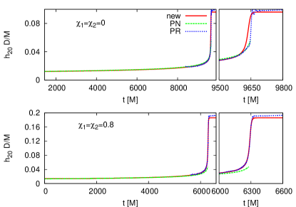
Figure 1: Comparison of $h_{20}$ waveforms among the current calculation result (marked with ‘new’), the post-Newtonian result (marked with ‘PN’) and the numerical relativity result (marked with ‘PR’) for binary black hole coalescence. The top row corresponds to spinless equal mass binary black hole. The bottom row corresponds to the spin aligned equal mass binary black hole with dimensionless spin parameter $\chi_{1}=\chi_{2}=0.8$. The right two plots are the enlargement of the merger part corresponding to the left two plots.

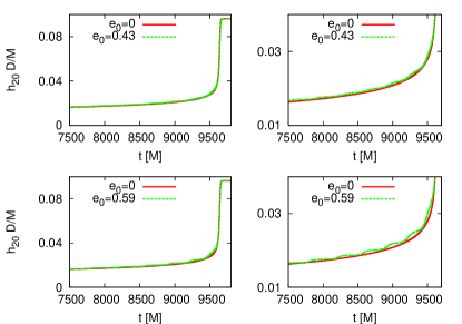
Figure 2: Memory waveform for eccentric binary black holes. The eccentricity $e_{0}$ means the initial eccentricity at reference frequency $Mf_{0}=0.002$ which is got by SEOBNRE model Liu et al. (2020). Here the quasi-circular one marked with $e_{0}=0$ corresponds to SXS:BBH:0070, the eccentric one marked with $e_{0}=0.43$ corresponds to SXS:BBH:1357 and the eccentric one marked with $e_{0}=0.59$ corresponds to SXS:BBH:1362. The right column shows the enlargement of the inspiral part of the waveform corresponding to the left column.

In the following we plug the SXS catalog results Caltech-Cornell-CITA for non-memory modes $h_{lm},m\neq 0$ into the Eq. (38) to calculate memory waveform $h_{l0}$. More specifically all $l=2,..,8$ with $m=-l,...,-1,1,...,l$ modes are used. As an example we show the comparison of the $h_{20}$ calculated through the above method to the numerical relativity result Pollney and Reisswig (2011) and post-Newtonian result Wiseman and Will (1991); Blanchet and Damour (1992); Thorne (1992); Favata (2009a, b, c, 2010, 2011); Nichols (2017); Cao and Han (2016) in the Fig. 1. Here the post-Newtonian result is got through the Eq. (8) of Cao and Han (2016) based on the SEOBNRE model Cao and Han (2017); Liu et al. (2020). The line corresponding to the post-Newtonian stops when the binary merger starts.

The Fig. 1 indicates that the result based on the current new method is consistent to the PN waveform quite well. But the deviation shows up near merger. The new result is also consistent to the numerical relativity result quite well. But at the time numerical relativity simulation starts (where the line marked with ‘PR’, Pollney and Reisswig, begins), the deviation between the PN waveform and new result is already clear. So the results Pollney and Reisswig (2011); Cao and Han (2016) through attaching the PN approximation to numerical relativity simulation may admit systematic error. In general, the new result and the PR result are quantitatively consistent.

The authors of Pollney and Reisswig (2011) have computed more than ten binary black hole systems with equal mass and aligned spin. We confirm that all of those results are consistent to our calculation in the current work similar to the Fig. 1.

Favata found strong effect of eccentricity on the memory waveform in Favata (2011) which results in oscillation of $h_{20}$. We confirm this result in the Fig. 2. But if we consider the GW memory amplitude $h^{tot}_{20}\equiv\left.h_{20}\right|_{-\infty}^{\infty}$ for binary black hole coalescence, the eccentricity effect is ignorable for almost equal mass binary black hole systems with eccentricity $e_{0}<0.6$ at reference frequency $Mf_{0}=0.002$ Cao and Han (2017); Liu et al. (2020).

The assumption (1) corresponds to the term

$$h^{1}_{l0}\bigg{|}_{t_{1}}^{t_{2}}=\sqrt{\frac{(l-2)!}{(l+2)!}}D\sum_{l^{\prime}=2}^{\infty}\sum_{l^{\prime\prime}=2}^{\infty}\sum_{\mbox{\tiny$\begin{array}[]{c}m^{\prime}=-l^{\prime},\\ m^{\prime}\neq 0\end{array}$}}^{l^{\prime}}\sum_{\mbox{\tiny$\begin{array}[]{c}m^{\prime\prime}=-l^{\prime\prime},\\ m^{\prime\prime}\neq 0\end{array}$}}^{l^{\prime\prime}}$$ (45)

$$\Gamma_{l^{\prime}l^{\prime\prime}lm^{\prime}-m^{\prime\prime}0}\int_{t_{1}}^{t_{2}}\dot{h}_{l^{\prime}m^{\prime}}\dot{\bar{h}}_{l^{\prime\prime}m^{\prime\prime}}dt$$ (46)

of (38). We call the above term 1 and denote it as $h^{1}_{l0}$. The authors of Khera et al. (2020) considered the “linear” (or alternately “ordinary”) memory contribution which corresponds to the term

$$h^{2}_{l0}\bigg{|}_{t_{1}}^{t_{2}}=-\sqrt{\frac{(l-2)!}{(l+2)!}}\frac{4}{D}\left.\int\Psi_{2}^{\circ}[{}^{0}Y_{l0}]\sin\theta d\theta d\phi\right|_{t_{1}}^{t_{2}}$$ (47)

of (38). We call the above term 2 and denote it as $h^{2}_{l0}$. In addition our Eq. (38) includes instant contribution of $\dot{h}_{lm},m\neq 0$

$$h^{3}_{lm}\bigg{|}_{t_{1}}^{t_{2}}=\sqrt{\frac{(l-2)!}{(l+2)!}}\sum_{l^{\prime}=2}^{\infty}\sum_{l^{\prime\prime}=2}^{\infty}\sum_{m^{\prime}=-l^{\prime}}^{l^{\prime}}\sum_{m^{\prime\prime}=-l^{\prime\prime}}^{l^{\prime\prime}}\Gamma_{l^{\prime}l^{\prime\prime}lm^{\prime}-m^{\prime\prime}-m}$$

$$\times D\left(\dot{h}_{l^{\prime}m^{\prime}}(t_{2})\bar{h}_{l^{\prime\prime}m^{\prime\prime}}(t_{2})-\dot{h}_{l^{\prime}m^{\prime}}(t_{1})\bar{h}_{l^{\prime\prime}m^{\prime\prime}}(t_{1})\right).$$ (48)

We call the above term 3 and denote it as $h^{3}_{l0}$. We investigate the fractional contributions of these three terms respectively in the Fig. 3 for the four cases shown in the Fig. 1 and the Fig. 2. The “linear” memory (term 2) is always negligible. The term 3 contributes between 0.01% and 1%. And as expected when $t\rightarrow\infty$ the term 3 vanishes. Consequently the term 3 does not contribute to $h_{lm}^{\rm tot}$. These kind of behaviors for term 2 and term 3 are common for all binary black holes.

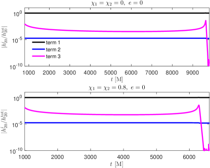
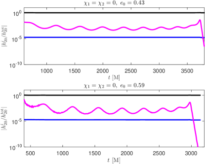
Figure 3: The fractional contributions of the three terms listed in Eqs. (46)-(48) for the four cases shown in Figs. 1 and 2.

IV GW memory for binary black hole coalescence

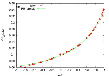
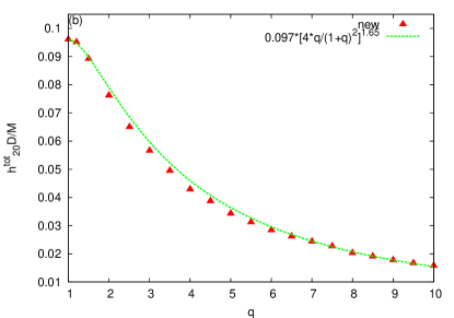
Figure 4: (a) Memory amplitude $h^{tot}_{20}$ of spin aligned equal mass binary black hole respect to the effective spin $\chi_{\rm eff}\equiv\frac{q\chi_{1z}+\chi_{2z}}{1+q}$. PR formula means the Eq. (49) (also the Eq. (8) of Pollney and Reisswig (2011)). (b) Memory amplitude of spinless binary black hole mergers respect to the mass ratio $q\equiv m_{1}/m_{2}$.

For equal mass spin aligned binary black hole systems, the authors of Pollney and Reisswig (2011) have found the relation between the GW memory amplitude $h^{tot}_{20}$ and the symmetric spin $\chi_{\rm eff}\equiv(m_{1}\chi_{1z}+m_{2}\chi_{2z})/M$ (Eq. (8) of Pollney and Reisswig (2011))

$$\frac{D}{M}h^{tot}_{20}= 0.0969+0.0562\chi_{\rm eff}+0.0340\chi_{\rm eff}^{2}+$$

$$0.0296\chi_{\rm eff}^{3}+0.0206\chi_{\rm eff}^{4}.$$ (49)

We confirm this formula based on SXS catalog in the Fig. 4(a). As pointed out by the authors of Pollney and Reisswig (2011) and also explained in Cao and Han (2016), we also confirm the memory amplitude $h^{tot}_{20}$ for equal mass spin aligned binary black hole is independent of the anti-symmetric part of the spin $\chi_{\rm A}\equiv\frac{\chi_{1z}-\chi_{2z}}{2}$.

In the Fig. 4(b), we investigate the GW memory amplitude of spinless binary black hole mergers respect to the mass ratio $q\equiv m_{1}/m_{2}$. Based on the PN approximation, Favata Seto (2009); Favata (2009b) showed the memory of the binary black hole with equal mass is about $\frac{1}{24\pi^{2}}\sqrt{\frac{1543}{70}}\approx 0.0198$ which is much less than the calculation result 0.097 here. And more Favata Seto (2009); Favata (2009b) estimated the memory is proportional to the symmetric mass ratio $\eta=\frac{q}{(1+q)^{2}}$. Here we find that it decreases much faster than Favata estimated. Instead it roughly behaves as $\eta^{1.65}$.

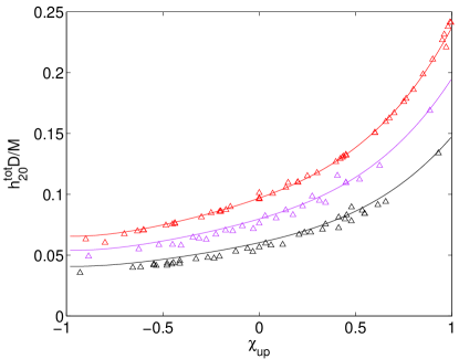
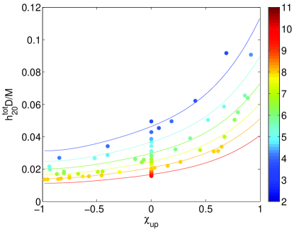
Figure 5: Memory amplitude $h^{tot}_{20}$ for generic spin aligned binary black hole respect to the spin hang-up parameter $\chi_{\rm up}$ which is defined in (50). The different colors mean different mass ratio. The left plot: red, cyan and black represent respectively $q=1$, $q=2$ and $q=3$. Right plot: The different lines from top to bottom represent the Eq. (51) with $q=4$, $q=5$, $q=6$, $q=7$, $q=8$ and $q=9.5$ respectively. The color of the points represent the different mass ratio indicated by the color bar.

For unequal mass spin aligned binary black holes, the Eq. (49) does not hold any more. In Liu et al. (2020) we found spin hang-up effect is the most important factor for gravitational waveform. Interestingly we find this statement is also correct for memory. Following Liu et al. (2020) we define a spin hang-up parameter as

$$\chi_{\rm up}\equiv\chi_{\rm eff}+\frac{3}{8}\sqrt{1-4\eta}\chi_{\rm A}.$$ (50)

This definition is different to the Eq. (7) of Liu et al. (2020). The current definition lets $\chi_{\rm up}$ go back to $\chi_{\rm eff}$ for equal mass binary black holes. Based on this spin hang-up parameter and the relationship between the GW memory amplitude and the mass ratio, we find the general behavior for generic spin aligned binary black hole systems can be expressed as

$$\frac{D}{M}h^{tot}_{20}= [0.0969+0.0562\chi_{\rm up}+0.0340\chi_{\rm up}^{2}+$$

$$0.0296\chi_{\rm up}^{3}+0.0206\chi_{\rm up}^{4}](4\eta)^{1.65}.$$ (51)

We validate the finding (51) in the Fig. 5. From this figure we can see the Eq. (51) does describe the main feature of the behavior. For systems with mass ratio between 2 and 4, the effect of $\chi_{\rm A}$ is stronger. So the points do not perfectly fall on the line. We suspect this is because only the combination of $\chi_{\rm A}$, $\sqrt{1-4\eta}$ and $\eta$ contributes to memory for $\chi_{\rm A}$ like the Eqs. (50) and (51). For the rest cases the Eq. (51) works very well. When the mass ratio increases, the effect of mass ratio decreases which can be seen in the Eq. (51). So after $q=3$ we use gradually larger and larger range to group numerical data in the Fig. 5.

V Discussion

We have proposed a new method to accurately calculate the GW memory for spin-aligned binary black holes. Our calculation indicates that the strongest GW memory amplitude for binary black hole merger corresponds to the fastest spinning aligned two equal mass black holes. And the amplitude is about $h^{tot}_{20}\approx 0.24\frac{M}{D}$. If the two black holes do not spin, the amplitude is about $h^{tot}_{20}\approx 0.1\frac{M}{D}$. Quantitatively we find that the memory amplitude can be described by spin hang-up parameter $\chi_{\rm up}$ and mass ratio $\eta$ quite well.

Based on our new method, it is straight forward to apply the technique of Varma et al. (2019) to construct a highly accurate numerical relativity surrogate model for GW memory. In the near future the detection of GW memory can be compared to the prediction by our method Khera et al. (2020) and give a test of general relativity.

References

- Zel’dovich and Polnarev (1974) Y. B. Zel’dovich and A. G. Polnarev, Soviet Astronomy 18, 17 (1974).
- Payne (1983) P. N. Payne, Phys. Rev. D 28, 1894 (1983), URL http://link.aps.org/doi/10.1103/PhysRevD.28.1894.
- Braginsky and Grishchuk (1985) V. B. Braginsky and L. P. Grishchuk, Sov. Phys. JETP 62, 427 (1985).
- Braginsky and Thorne (1987) V. B. Braginsky and K. S. Thorne, Nature 327, 123 (1987).
- Christodoulou (1991) D. Christodoulou, Phys. Rev. Lett. 67, 1486 (1991), URL https://link.aps.org/doi/10.1103/PhysRevLett.67.1486.
- Frauendiener (1992) J. Frauendiener, Classical and Quantum Gravity 9, 1639 (1992).
- Thorne (1992) K. S. Thorne, Phys. Rev. D 45, 520 (1992), URL http://link.aps.org/doi/10.1103/PhysRevD.45.520.
- Wiseman and Will (1991) A. G. Wiseman and C. M. Will, Phys. Rev. D 44, R2945 (1991), URL http://link.aps.org/doi/10.1103/PhysRevD.44.R2945.
- Blanchet and Damour (1992) L. Blanchet and T. Damour, Phys. Rev. D 46, 4304 (1992), URL http://link.aps.org/doi/10.1103/PhysRevD.46.4304.
- Favata (2009a) M. Favata, Phys. Rev. D 80, 024002 (2009a), URL http://link.aps.org/doi/10.1103/PhysRevD.80.024002.
- Favata (2009b) M. Favata, The Astrophysical Journal Letters 696, L159 (2009b).
- Favata (2009c) M. Favata, in Journal of Physics: Conference Series (IOP Publishing, 2009c), vol. 154, p. 012043.
- Favata (2010) M. Favata, Classical and Quantum Gravity 27, 084036 (2010).
- Favata (2011) M. Favata, Phys. Rev. D 84, 124013 (2011), URL https://link.aps.org/doi/10.1103/PhysRevD.84.124013.
- Nichols (2017) D. A. Nichols, Phys. Rev. D 95, 084048 (2017), URL https://link.aps.org/doi/10.1103/PhysRevD.95.084048.
- Talbot et al. (2018) C. Talbot, E. Thrane, P. D. Lasky, and F. Lin, Phys. Rev. D 98, 064031 (2018), URL https://link.aps.org/doi/10.1103/PhysRevD.98.064031.
- Khera et al. (2020) N. Khera, B. Krishnan, A. Ashtekar, and T. De Lorenzo, arXiv e-prints arXiv:2009.06351 (2020), eprint 2009.06351.
- Lasky et al. (2016) P. D. Lasky, E. Thrane, Y. Levin, J. Blackman, and Y. Chen, Phys. Rev. Lett. 117, 061102 (2016), URL https://link.aps.org/doi/10.1103/PhysRevLett.117.061102.
- Boersma et al. (2020) O. M. Boersma, D. A. Nichols, and P. Schmidt, Phys. Rev. D 101, 083026 (2020), URL https://link.aps.org/doi/10.1103/PhysRevD.101.083026.
- Hübner et al. (2020) M. Hübner, C. Talbot, P. D. Lasky, and E. Thrane, Phys. Rev. D 101, 023011 (2020), URL https://link.aps.org/doi/10.1103/PhysRevD.101.023011.
- Ebersold and Tiwari (2020) M. Ebersold and S. Tiwari, Phys. Rev. D 101, 104041 (2020), URL https://link.aps.org/doi/10.1103/PhysRevD.101.104041.
- Baker et al. (2007) J. G. Baker, M. Campanelli, F. Pretorius, and Y. Zlochower, Classical and Quantum Gravity 24, S25 (2007), URL https://doi.org/10.1088%2F0264-9381%2F24%2F12%2Fs03.
- Abbott et al. (2016) B. P. Abbott et al. (LIGO Scientific Collaboration and Virgo Collaboration), Phys. Rev. Lett. 116, 061102 (2016), URL https://link.aps.org/doi/10.1103/PhysRevLett.116.061102.
- Abbott et al. (2019) B. P. Abbott et al. (LIGO Scientific Collaboration and Virgo Collaboration), Phys. Rev. X 9, 031040 (2019), URL https://link.aps.org/doi/10.1103/PhysRevX.9.031040.
- Pollney and Reisswig (2011) D. Pollney and C. Reisswig, The Astrophysical Journal Letters 732, L13 (2011).
- Mitman et al. (2020) K. Mitman, J. Moxon, M. A. Scheel, S. A. Teukolsky, M. Boyle, N. Deppe, L. E. Kidder, and W. Throwe, Phys. Rev. D 102, 104007 (2020), URL https://link.aps.org/doi/10.1103/PhysRevD.102.104007.
- Mitman et al. (2020) K. Mitman, D. Iozzo, N. Khera, M. Boyle, T. De Lorenzo, N. Deppe, L. E. Kidder, J. Moxon, H. P. Pfeiffer, M. A. Scheel, et al., arXiv e-prints arXiv:2011.01309 (2020), eprint 2011.01309.
- Seto (2009) N. Seto, Monthly Notices of the Royal Astronomical Society: Letters 400, L38 (2009).
- Van Haasteren and Levin (2010) R. Van Haasteren and Y. Levin, Monthly Notices of the Royal Astronomical Society 401, 2372 (2010).
- Pshirkov et al. (2010) M. Pshirkov, D. Baskaran, and K. Postnov, Monthly Notices of the Royal Astronomical Society 402, 417 (2010).
- Cordes and Jenet (2012) J. Cordes and F. Jenet, The Astrophysical Journal 752, 54 (2012).
- Madison et al. (2014) D. Madison, J. Cordes, and S. Chatterjee, The Astrophysical Journal 788, 141 (2014).
- Arzoumanian et al. (2015) Z. Arzoumanian, A. Brazier, S. Burke-Spolaor, S. J. Chamberlin, S. Chatterjee, B. Christy, J. M. Cordes, N. J. Cornish, P. B. Demorest, X. Deng, et al., The Astrophysical Journal 810, 150 (2015), URL https://doi.org/10.1088%2F0004-637x%2F810%2F2%2F150.
- McNeill et al. (2017) L. O. McNeill, E. Thrane, and P. D. Lasky, Phys. Rev. Lett. 118, 181103 (2017), URL https://link.aps.org/doi/10.1103/PhysRevLett.118.181103.
- Divakarla et al. (2019) A. K. Divakarla, E. Thrane, P. D. Lasky, and B. F. Whiting (2019), eprint 1911.07998.
- Bondi et al. (1962) H. Bondi, M. Van der Burg, and A. Metzner, Proceedings of the Royal Society of London. Series A. Mathematical and Physical Sciences 269, 21 (1962).
- Sachs (1962) R. K. Sachs, Proceedings of the Royal Society of London. Series A. Mathematical and Physical Sciences 270, 103 (1962).
- Penrose and Rindler (1988) R. Penrose and W. Rindler, Spinors and space-time: Volume 1 and Volume 2 (Cambridge University Press, 1988).
- Held et al. (1970) A. Held, E. T. Newman, and R. Posadas, Journal of Mathematical Physics 11, 3145 (1970).
- Brügmann et al. (2008) B. Brügmann, J. A. González, M. Hannam, S. Husa, U. Sperhake, and W. Tichy, Phys. Rev. D 77, 024027 (2008), URL https://link.aps.org/doi/10.1103/PhysRevD.77.024027.
- He and Cao (2015) X. He and Z. Cao, International Journal of Modern Physics D 24, 1550081 (2015).
- He et al. (2016) X. He, Z. Cao, and J. Jing, International Journal of Modern Physics D 25, 1650086 (2016).
- Sun et al. (2019) B. Sun, Z. Cao, and X. He, SCIENCE CHINA Physics, Mechanics & Astronomy 62, 40421 (2019).
- Buonanno et al. (2007) A. Buonanno, G. B. Cook, and F. Pretorius, Phys. Rev. D 75, 124018 (2007), URL https://link.aps.org/doi/10.1103/PhysRevD.75.124018.
- Maggiore (2008) M. Maggiore, Gravitational waves: Volume 1: Theory and experiments, vol. 1 (Oxford university press, 2008).
- Cao et al. (2008) Z. Cao, H.-J. Yo, and J.-P. Yu, Phys. Rev. D 78, 124011 (2008), URL https://link.aps.org/doi/10.1103/PhysRevD.78.124011.
- Ashtekar et al. (2019) A. Ashtekar, T. De Lorenzo, and N. Khera (2019), eprint 1906.00913.
- Varma et al. (2020) V. Varma, M. Isi, and S. Biscoveanu (2020), eprint 2002.00296.
- Calderón Bustillo et al. (2018) J. Calderón Bustillo, J. A. Clark, P. Laguna, and D. Shoemaker, Phys. Rev. Lett. 121, 191102 (2018), URL https://link.aps.org/doi/10.1103/PhysRevLett.121.191102.
- Gerosa and Moore (2016) D. Gerosa and C. J. Moore, Phys. Rev. Lett. 117, 011101 (2016), URL https://link.aps.org/doi/10.1103/PhysRevLett.117.011101.
- Liu et al. (2020) X. Liu, Z. Cao, and L. Shao, Phys. Rev. D 101, 044049 (2020), URL https://link.aps.org/doi/10.1103/PhysRevD.101.044049.
- (52) Caltech-Cornell-CITA, binary black hole simulation results, http://www.black-holes.org/waveforms.
- Cao and Han (2016) Z. Cao and W.-B. Han, Classical and Quantum Gravity 33, 155011 (2016).
- Cao and Han (2017) Z. Cao and W.-B. Han, Phys. Rev. D 96, 044028 (2017), URL https://link.aps.org/doi/10.1103/PhysRevD.96.044028.
- Varma et al. (2019) V. Varma, S. E. Field, M. A. Scheel, J. Blackman, D. Gerosa, L. C. Stein, L. E. Kidder, and H. P. Pfeiffer, Phys. Rev. Research 1, 033015 (2019), URL https://link.aps.org/doi/10.1103/PhysRevResearch.1.033015.