Leveraging Domain Relations for Domain Generalization

Abstract

Distribution shift is a major challenge in machine learning, as models often perform poorly during the test stage if the test distribution differs from the training distribution. In this paper, we focus on domain shifts, which occur when the model is applied to new domains that are different from the ones it was trained on, and propose a new approach called D³G. Unlike previous approaches that aim to learn a single model that is domain invariant, D³G learns domain-specific models by leveraging the relations among different domains. Concretely, D³G learns a set of training-domain-specific functions during the training stage and reweights them based on domain relations during the test stage. These domain relations can be directly derived or learned from fixed domain meta-data. Under mild assumptions, we theoretically proved that using domain relations to reweight training-domain-specific functions achieves stronger generalization compared to averaging them. Empirically, we evaluated the effectiveness of D³G using both toy and real-world datasets for tasks such as temperature regression, land use classification, and molecule-protein interaction prediction. Our results showed that D³G consistently outperformed state-of-the-art methods, with an average improvement of 10.6% in performance.

1 Introduction

Distribution shift is a common problem in real-world applications (Gulrajani & Lopez-Paz, 2021; Koh et al., 2021a). When the test distribution differs from the training distribution, these models often experience a significant decline in performance. In this paper, we specifically focus on domain shifts and expect a well-trained machine learning model should be able to generalize to unseen domains without accessing additional examples from these unseen domains during the training stage. An example of this is predicting how well a drug will bind to a specific target protein. In drug discovery, each protein can determine a specific biological domain (Ji et al., 2022), and one open challenge is to train a robust model that can be adapted for novel biological domains, such as drug-target binding affinity prediction with the unseen proteins.

Prior domain generalization approaches often try to learn a single model that is domain invariant (Arjovsky et al., 2019; Krueger et al., 2021b; Yao et al., 2022a; Sun & Saenko, 2016; Li et al., 2018a), and differ in the techniques they use to encourage invariance. These methods have shown promise but there remains significant room for improvement on real-world distribution shift problems such as those in the WILDS benchmark (Koh et al., 2021b). Unlike the approach of learning a single domain-invariant model, we posit that models may perform better if they were specialized to a given domain. Benefits from learning multiple domain-specific models could arise for a variety of reasons. First, it may simply be difficult to train a general model that works for all domains, e.g. due to challenges in multi-task optimization. Second, while domain generalization is typically cast as a covariate shift problem, real-world problems could exhibit concept shift across domains. Third, if different domains have strong correlations with “non-causal” or non-general features, domain-specific models can leverage these features to make more accurate predictions. While there are clearly some possible benefits to learning domain-specific models, it remains unclear how to construct a domain-specific model for a new domain seen at test time, without any training data for that domain.

To resolve this challenge, our key hypotheses are that similar domains have similar predictive functions and the test domain is sufficiently similar to some of the training domains. Based on these hypotheses, we can attain a good model for the test domain by leveraging information about the relationship between different domains, including the relationship between the test domain and the training domains. This relational information indicates how similar two domains are to one another, and can often be derived from meta-data, such as protein-protein interactions or geographical proximity. While one natural approach would be to fine-tune a generic model on the reweighted training data during test time, this has two major drawbacks: first, in real-world applications, it may not be possible to access data from all training domains due to privacy concerns; second, fine-tuning the generic model for every test domain is time-consuming, especially when there are a large number of test domains.

To overcome these challenges, we propose a novel approach called D³G (leveraging domain distances for domain generalization) to learn a set of diverse, training domain-specific functions during the training stage, where each function corresponds to a single domain or a set of domains with similar properties. For each test domain, D³G leverages the domain relations to weight these training domain-specific functions and perform inference. The domain relations can be both directly derived and learned from fixed domain meta-data. Additionally, we also introduce a consistency regularizer that takes into account domain relations to aid in training domain-specific predictors for data-insufficient domains.

With mild assumptions, our theoretical analysis shows that D³G can achieve better domain generalization by using domain relations to reweight training domain-specific functions, compared with averaging them. Empirically, we thoroughly evaluate D³G on both toy and real-world datasets with natural domain shifts, including temperature regression, land use classification, and molecule-protein interaction prediction. The results show that D³G outperforms the best prior method, with an average improvement of 10.6%.

2 Preliminaries

Out-of-Distribution Generalization. In this paper, we consider the problem of predicting the label $y\in\mathcal{Y}$ based on the input feature $x\in\mathcal{X}$. Given training data distributed according to $P^{tr}$, we train a model $f$ parameterized by $\theta\in\Theta$ using a loss function $\ell$. Traditional empirical risk minimization (ERM) optimizes the following objective:

$$\small\arg\min_{\theta\in\Theta}\mathbb{E}_{(x,y)\sim P^{tr}}[\ell(f_{\theta}(x),y)].$$ (1)

The trained model is evaluated on a test set from a test distribution $P^{ts}$. When distribution shift occurs, the training and test distributions are different, i.e., $P^{tr}\neq P^{ts}$.

Concretely, following Koh et al. (2021b), we consider a setting in which the overall data distribution is drawn from a set of domains $\mathcal{D}=\{1,\ldots,D\}$, where each domain $d\in\mathcal{D}$ is associated with a domain-specific data distribution $P_{d}$ over a set $(X,Y,d)=\{(x_{i},y_{i},d)\}_{i=1}^{n_{d}}$. The training distribution and test distribution are both considered to be mixture distributions of the $D$ domains, i.e., $P^{tr}=\sum_{d\in\mathcal{D}}r_{d}^{tr}P_{d}$ and $P^{ts}=\sum_{d\in\mathcal{D}}r_{d}^{ts}P_{d}$, respectively, where ${r_{d}^{tr}}$ and ${r_{d}^{ts}}$ denote the mixture probabilities in the training set and test set, respectively. We also define the training domains and test domains as $\mathcal{D}^{tr}=\{d\in\mathcal{D}|r_{d}^{tr}>0\}$ and $\mathcal{D}^{ts}=\{d\in\mathcal{D}|r_{d}^{ts}>0\}$, respectively. In this paper, we consider domain shifts, where the test domains are disjoint from the training domains, i.e., $\mathcal{D}^{tr}\cap\mathcal{D}^{ts}=\emptyset$. In addition, the domain ID of training and test datapoints are available.

Domain Relations. In this study, we aim to deal with domain shift by leveraging domain relations. Domain relations refer to the similarity or relatedness between different domains. As an example, let’s consider the task of protein-ligand binding affinity prediction, where each protein is treated as a separate domain. If two proteins have similar protein sequences or belong to the same protein family, they can be considered related domains. To formalize domain relations, we define an undirected domain similarity matrix $\mathcal{A}=\{a_{ij}\}_{i,j=1}^{D}$, where each element $a_{ij}$ represents the strength of the relation between domains $i$ and $j$.

3 Leveraging Domain Relations for Domain Generalization

We now describe the proposed method – D³G (leveraging domain distances for domain generalization). The goal of D³G is to improve handling of domain shifts by constructing domain-specific models. During training, a multi-headed network is used to learn domain-specific functions, with each head associated with a different training domain (Figure 1(a)). A consistency loss is also introduced to address the challenge of insufficient training data for certain domains (Figure 1(c)). During testing, test domain-specific models are constructed for inference by reweighing the training domain-specific models, taking into account the similarity between the training and test domains (Figure 1(d)). Relations between domains are extracted directly from domain meta-data and refined through learning from the same meta-data (Figure 1(b)). In the remainder of this section, we will explain in more detail the processes of building domain-specific models during training and inference, as well as how to obtain domain relations.

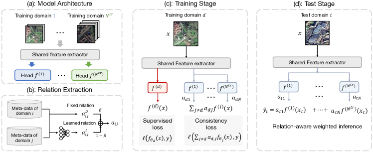
Figure 1: An illustration of D³G. (a) The multi-headed architecture of D³G, where each training domain is associated with a single head for prediction. (b) The relation extraction module, where fixed relations are extracted from domain meta-data and refined through learning from the same meta-data. (c) The training stage of D³G, where $x$ represents a single example from domain $d$, and the loss is composed of both a supervised loss and a consistency loss. (d) The test stage, where the weighting of all training domain-specific functions is used to perform inference for each test example.

3.1 Building Domain-Specific Models

In this section, we present the details of D³G for learning a collection of domain-specific functions during the training stage and leveraging these functions for relational inference during the test stage.

Training Stage. During training, we use a multi-headed neural network with $N^{tr}$ heads, where $N^{tr}$ represents the number of training domains. For simplicity, we use a separate head for each training domain in the presented method, but it is also possible to have domains with similar properties share a single head.

Given an input datapoint ($x$, $y$) from domain $d$, the prediction made by the $d$-th head is denoted as $f^{(d)}(x)$. To ensure that each datapoint has a low predictive risk when using the corresponding head, we minimize the following loss:

$$\mathcal{L}_{pred}=\mathbb{E}_{d\in\mathcal{D}^{tr}}\mathbb{E}_{(x,y)\sim P_{d}}[\ell(f^{(d)}(x),y)].$$ (2)

It is possible that some training domains may not have a large amount of data compared to the entire training set, making it difficult to train domain-specific predictors. By assuming that similar domains likely have similar predictive functions, we introduce a relation-aware consistency regularizer to strengthen the correlations between the training domain-specific functions. Concretely, for each example ($x$, $y$) from domain $d$, we aim to get its prediction by using domain relations to weight the predictions made by all training predictors except its corresponding predictor, i.e., function $f^{(d)}$. We formulate the relation-aware consistency loss as:

$$\small\mathcal{L}_{rel}=\mathbb{E}_{d\in\mathcal{D}^{tr}}\mathbb{E}_{(x,y)\sim P_{d}}\left[\ell\left(\frac{\sum_{j=1,j\neq d}^{N^{tr}}a_{dj}f^{(j)}(x)}{\sum_{k=1,k\neq d}^{N^{tr}}a_{dk}},y\right)\right].$$ (3)

This loss encourages the groundtruth to be consistent with the weighted average prediction obtained from all other training predictors, using the domain relations to weight their contributions. By doing so, the regularizer encourages the model to: (1) rely more on predictions made by similar domains, and less on predictions made by dissimilar domains; (2) strengthen the relations between predictors and help training predictors for domains with insufficient data.

To incorporate the relation-aware consistency loss into our training process, we add it to the predictive loss term in Eqn. (2) and obtain the final loss as:

$$\small\mathcal{L}=\mathcal{L}_{pred}+\lambda\mathcal{L}_{rel},$$ (4)

where $\lambda$ is used to balance these two loss terms.

Test Stage. During the testing phase, D³G constructs test domain-specific models based on the same assumption that similar domains have similar predictive functions. Concretely, we weight all training domain-specific functions and perform inference for each test domain $t$ by weighting the predictions from the corresponding prediction heads. Specifically, for each test datapoint $x$ drawn from the test distribution $P_{t}$, D³G makes a prediction as follows:

$$\small\hat{y}=\frac{\sum_{d=1}^{N^{tr}}a_{dt}f^{(d)}(x)}{\sum_{k=1}^{N^{tr}}a_{kt}},$$ (5)

where $a_{dt}$ represents the strength of the relation between the test domain $t$ and the training domain $d$. According to Eqn. (5), for each test domain, training domains with stronger relations play a more important role in prediction. This allows D³G to provide more accurate predictions by leveraging the knowledge from related domains.

3.2 Extracting and Refining Domain Relations

In this section, we discuss how to obtain the pairwise similarity matrix $\mathcal{A}=\{a_{ij}\}_{i,j=1}^{D}$ between different domains. Domain relations can be first collected from or derived from domain meta-data. For example, in drug-target binding affinity prediction task, where each protein is treated as a domain, we can use a protein-protein interaction network to model the relations between different proteins. Another scenario is, if we aim to predict the land use category using satelite images (Koh et al., 2021b), and each country is treated as a domain, we can use geographical proximity to model the relations among countries. The relation between domains $i$ and $j$ that is directly collected from fixed domain meta-data is defined as $a_{ij}^{g}$.

One potential issue with directly collecting domain relations from fixed domain meta-data is that these fixed relations may not fully reflect accurate application-specific domain relations. For example, geographical proximity can be used in any applications with spatial domain shifts, but it is hard to pre-define how strongly two nearby regions are related for different applications. To address this issue and refine the fixed relations, we propose learning the domain relations from domain meta-data using a similarity metric function. Specifically, given domain meta-data $m_{i}$ and $m_{j}$ of domains $i$ and $j$, we use a two layer neural network $g$ to learn the corresponding domain representations $g(m_{i})$ and $g(m_{j})$. Following Chen et al. (2020), we compute the similarity between domains $i$ and $j$ with a multi-headed similarity layer, which is formulated as follows:

$$\small a^{l}_{ij}=\frac{1}{R}\sum_{r=1}^{R}cos(w_{r}\odot g(m_{i}),w_{r}\odot g(m_{j})),$$ (6)

where $\odot$ denotes the Hadamard product and $R$ is the number of heads. The collection of learnable weight vectors $\{w_{r}\}_{r=1}^{R}$ has the same dimension as the domain representation $g(m_{i})$ and is used to highlight different dimensions of the vectors.

To combine the fixed and learned relations, we propose using a weighted sum. Specifically, we define the final relation between domains $i$ and $j$ as a weighted sum of the fixed relation $a_{ij}^{g}$ and the learned relation $a_{ij}^{l}$, as follows:

$$\small a_{ij}=\beta a_{ij}^{g}+(1-\beta)a_{ij}^{l},$$ (7)

where $0\leq\beta\leq 1$ is a hyperparameter that controls the importance of both kinds of relations. By tuning $\beta$, we can balance the contribution of the fixed and learned relations to the final relation between domains. The final domain relations are used in the consistency regularization and testing stage. To summary, the pseudocodes of training and testing stages of D³G is detailed in Alg. 1.

Algorithm 1 Training and Test Procedure of D³G

0:  Training and test data, relation combining coefficient $\beta$, loss balanced coefficient $\lambda$, meta-data $\{m_{d}\}_{d=1}^{D}$ of all domains, learning rate $\gamma$

1:  /* Training stage */

2:  Initialize all learnable parameters

3:  Extract fixed relations $\{a_{ij}^{g}\}_{i,j=1}^{N^{tr}}$.

4:  while not converge do

5:     Computed learned relations $\{a_{ij}^{l}\}_{i,j=1}^{N^{tr}}$ by Eqn. (6).

6:     Obtained the final domain relations by Eqn. (7).

7:     for each example ($x$, $y$, $d$) do

8:        Calculated supervised loss $\mathcal{L}_{pred}$ by Eqn. (2).

9:        Computed consistency loss $\mathcal{L}_{rel}$ by Eqn. (3) using domain relations.

10:     end for

11:     Update learnable parameters with learning rate $\gamma$.

12:  end while

13:  /* Test stage */

14:  for each test domain $t$ do

15:     Computed fixed and learned relations and obtained the final relations with training domains $\{a_{dt}\}_{d=1}^{N^{tr}}$

16:     for each example ($x$, $y$, $t$) do

17:        Computed the prediction $\hat{y}$ by Eqn. (5).

18:     end for

19:  end for

4 Theoretical Analysis

In this section, we analyze the benefits of utilizing domain relations to bridge the gap between training and test domains in the presence of domain shift. Our proposed model, D³G, utilizes a multi-headed network where the feature extractor is shared among all training domains, but different domain-specific heads are used. In our theoretical analysis, for an input datapoint ($x$, $y$) from domain $d$, we rearrange the predictive function as:

$$\small y=f^{(d)}(x)+\epsilon:=h^{(d)}(e(x))+\epsilon,$$ (8)

where $h^{(d)}(\cdot)$ and $e(\cdot)$ represent the head of domain $d$ and feature extractor, respectively. $\epsilon$ is a noise term which is assumed to be sub-Gaussian with mean 0 and variance $\sigma^{2}$.

During the test process, we assume that for the test domain $t$, the outcome prediction function $f^{(t)}(x)$ is estimated by

$$\small\hat{f}^{(t)}(x)=\hat{h}^{(t)}(e(x)),$$ (9)

where $\hat{h}^{(t)}=\frac{\sum_{i=1}^{N^{tr}}w_{it}\hat{h}^{(i)}}{\sum_{k=1}^{N^{tr}}w_{kt}}$, where $\hat{h}^{(i)}$ represents the learned head for domain $i$. In our theoretical analysis, we consider the case where $w_{it}=\mathbbm{1}\{a_{it}<B\}$ for some hyperparameter $B>0$. Here, we define $a_{it}$ is the original relations between domain $i$ and $t$. If the denominator is $0$, we define $\hat{h}^{(t)}=0$.

To facilitate the theoretical analysis, we first assume that the domain relations indeed captures the similarity of domains, i.e., there exists a universal constant $G$, such that

$$\|h^{(i)}-h^{(j)}\|_{\infty}\leq G\cdot a_{ij}.$$ (10)

Moreover, we assume that for each domain $d$, there is a domain representation $Z^{(d)}\in[0,1]^{r}$ such that $a_{ij}=\|Z^{(i)}-Z^{(j)}\|$ and $Z^{(d)}$ uniformly distributed on $[0,1]^{r}$. In addition, we assume that for each training domain $d$, $\hat{h}^{(d)}$ is well-learned such that $\mathbb{E}[(\hat{h}^{(d)}(e(x))-h^{(d)}(e(x)))^{2}]=O(\frac{C(\mathcal{H})}{n_{d}})$, where $C(\mathcal{H})$ is the Rademacher complexity of the function class $\mathcal{H}$. We then have the following theorem.

Theorem 4.1.

Suppose we have the number of examples $n_{d}\gtrsim n$ for all training domain $d\in\mathcal{D}^{tr}$. If the loss function $\ell$ is Lipschitz with respect to the first argument, then for the test domain $t$, the excess risk satisfies

$$\small\begin{split}\mathbb{E}_{(x,y)\sim P_{t}}[\ell(\hat{f}^{(t)}(x),y)]&-\mathbb{E}_{(x,y)\sim P_{t}}[\ell(f^{(t)}(x),y)]\\ &\lesssim B+\sqrt{\frac{C(\mathcal{H})/n}{N^{tr}B^{r}}}.\end{split}$$ (11)

If we further take $B\asymp(\frac{C(\mathcal{H})/n}{N^{tr}})^{\frac{1}{r+2}}$, we then have

$$\small\begin{split}\mathbb{E}_{(x,y)\sim P_{t}}[\ell(\hat{f}^{(t)}(x),y)]&-\mathbb{E}_{(x,y)\sim P_{t}}[\ell(f^{(t)}(x),y)]\\ &\lesssim\left(\frac{C(\mathcal{H})/n}{N^{tr}}\right)^{\frac{1}{r+2}}.\end{split}$$ (12)

The theorem above implies that by taking into account the domain relations, the more training tasks we have, the smaller the excess risk will be. Additionally, the result shows that even in the extreme case where the test domain is seen during training, our method can still achieve a smaller test error than using ERM solely on this domain as long as $N^{tr}\gtrsim(n/C(\mathcal{H}))^{r}$, in which case we have $(\frac{C(\mathcal{H})/n}{N^{tr}})^{\frac{1}{r+2}}\lesssim\sqrt{C(\mathcal{H})/n}$ (ERM risk). The detailed proofs are in Appendix A.1.

In the following, we present a proposition, showing that obtaining a good relation $A$ is important in improving generalization error. Here we assume a ill-defined similarity matrix as $\tilde{A}=\{\tilde{a}_{ij}\}_{i,j=1}^{D}$, where each $\tilde{a}_{ij}=0$, i.e., all training domains are equally important. We compare the well-defined similarity matrix $A$ and ill-defined $\tilde{A}$ in the following proposition:

Proposition 4.2.

Under the same conditions as Theorem 4.1, suppose that all $\tilde{a}_{ij}=0$ and consider the function class $\mathcal{H}\in\{h:\|h^{(i)}-h^{(j)}\|_{\infty}\leq G\cdot\|Z^{(i)}-Z^{(j)}\|$ for all $i,j\in\mathcal{D}\}$. Define the excess risk with similarity matrix $A$ by $R_{h}(\hat{f}^{(t)},A)=\mathbb{E}_{(x,y)\sim P_{t}}[\ell(\hat{f}^{(t)}(x),y;A)]-\mathbb{E}_{(x,y)\sim P_{t}}[\ell(f^{(t)}(x),y;A)]$, we then have

$$\inf_{\hat{f}^{(t)}}\sup_{h\in\mathcal{H}}R_{h}(\hat{f}^{(t)},A)<\inf_{\hat{f}^{(t)}}\sup_{h\in\mathcal{H}}R_{h}(\hat{f}^{(t)},\tilde{A}).$$ (13)

The above proposition suggests that by utilizing good domain relations, we can achieve better generalization than treating all training domains equally. The detailed proof of the above proposition is in Appendix A.2.

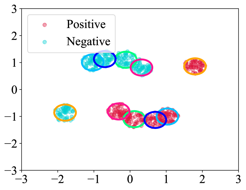
(a) Training Distribution

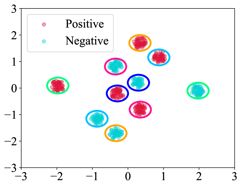
(b) Test Distribution

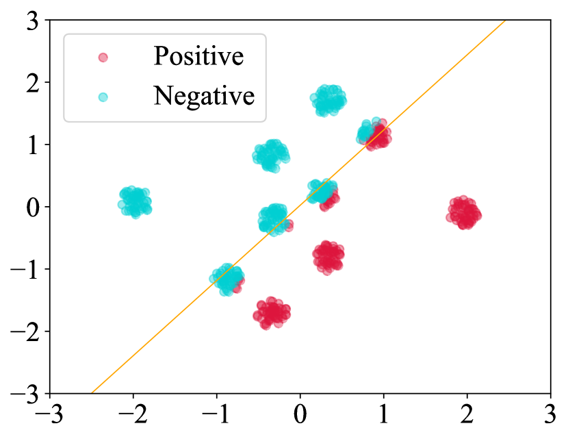
(c) GroupDRO

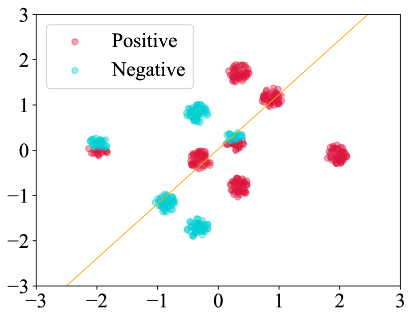
(d) D³G

Model	ERM	GroupDRO	IRM	IB-IRM	IB-ERM	V-REx	DANN	CORAL	MMD	CAD	SelfReg	Mixup	LISA	D3G (ours)
Accuracy	44.0%	47.7%	43.9%	45.4%	43.1%	44.0%	43.1%	43.5%	41.3%	43.3%	40.7%	41.3%	47.4%	77.5%

Figure 2: Results of domain shifts on toy binary classification task (DG-15). Top figures (a) and (b) illustrate the training and test data distributions, where datapoints in ciricles with the same color originate from the same domain. Top figures (c) and (d) show the predicted distribution of the strongest baseline (GroupDRO) and D³G. Bottom Table reports averaged accuracy over all test domains (see full table with standard deviation in Appendix E). We bold the best results and underline the second best results.

5 Experiments

In this section, we conduct a series of experiments to evaluate the effectiveness of D³G. Our goals are to answer the following questions: Q1: Compared to prior methods, can D³G improve robustness to domain shifts (Section 5.1 and Section 5.2)? Q2: Which aspects of D³G are the most important for improving robustness (Section 5.3)? Q3: How does D³G perform compared with domain-specific fine-tuning (Section 5.4)? Q4: Does relation learning in D³G successfully refine fixed relations and learn application-specific information (Section 5.5)?

Our main points of comparison are general-purpose methods with different learning strategies and categories including (1) vanilla: ERM (Vapnik, 1999), (2) distributionally robust optimization: GroupDRO (Sagawa et al., 2020), (3) invariant learning: IRM (Arjovsky et al., 2019), IB-IRM (Ahuja et al., 2021b), IB-ERM (Ahuja et al., 2021b), V-REx (Krueger et al., 2021b), DANN (Ganin et al., 2016a), CORAL (Sun & Saenko, 2016), MMD (Li et al., 2018b), CAD (Ruan et al., 2022), SelfReg (Kim et al., 2021), Mixup (Xu et al., 2020), LISA (Yao et al., 2022a). We provide detailed descriptions in Appendix B.

For a fair comparison, we adopt the same model architectures and use the same input ($x,y,d$) for all approaches. Specifically, we incorporate domain meta-data as features for all baselines. All hyperparameters are selected via cross-validation. Detailed setups are provided in Appendix C.

5.1 Illustrative Toy Task

Dataset Descriptions. Following Xu et al. (2022), we use the DG-15 dataset, a synthetic binary classification dataset with 15 domains. In each domain $d$, a two-dimensional key point $x_{d}=(x_{d,1},x_{d,2})$ is randomly selected in the two-dimensional space, and the domain meta-data is represented by the angle of the point (i.e., $\arctan{(\frac{x_{d,2}}{x_{d,1}})}$). 50 positive and 50 negative datapoints are generated from two Gaussian distributions $\mathcal{N}(x_{d},\mathbf{I})$ and $\mathcal{N}(-x_{d},\mathbf{I})$ respectively. In DG-15, we construct the fixed relations between domain $i$ and $j$ as the angle difference between key points $x_{i}$ and $x_{j}$, i.e., $a^{g}_{ij}=\arctan{(\frac{x_{j,2}}{x_{j,1}})}-\arctan{(\frac{x_{i,2}}{x_{i,1}})}$. The number of training, validation, and test domains are all set as 5. We visualize the training and test data in Figure 2(a) and 2(b).

Results and Analysis. The performance of D³G on DG-15 is reported in the bottom table in Figure 2. It outperforms other methods by about 30%. Previous methods also perform worse than random guessing, highlighting the importance of incorporating domain relations to transfer information between related domains. To further understand the performance gains, Figures 2(c) and 2(d) illustrate the predictions from the strongest prior method (GroupDRO) and D³G. GroupDRO learns a nearly linear decision boundary that overfits the training domains and fails to generalize on the shifted test domains. In contrast, D³G leverages domain meta-data and generalizes well to test domains except for one without a nearby training domain.

5.2 Real World Domain Shifts

Datasets Descriptions. In this subsection, we briefly describe three datasets with natural distribution shifts and Appendix D provides additional details.

• TPT-48. TPT-48 is a real-world weather prediction dataset from the nClimDiv and nClimGrid (Vose et al., 2014) databases, which contains the monthly average temperature for the 48 contiguous states in the US from 2008 to 2019. The data is processed following Washington Post (cci, 2020), and the focus is on a regression task that forecasts the next 6 months’ temperature based on the previous 6 months’ temperature. Each state is treated as a domain, and the domain meta-data is defined as the geographical location of each state, i.e., the latitude and longitude of its geographic center. In TPT-48, a 0/1 adjacency matrix is used as the fixed domain similarity matrix, where $a^{g}_{ij}=1$ represents that states $i$ and $j$ are geographically connected. Following Xu et al. (2022), we consider two dataset splits: I. N (24) $\rightarrow$ S (24): generalizing from the 24 states in the north to the 24 states in the south; II. E (24) $\rightarrow$ W (24): generalizing from the 24 states in the east to the 24 states in the west.

• FMoW. The FMoW task is to predict the building or land use category based on satellite images. For each region, we use geographical information as domain meta-data, which is defined as the average latitude and longitude coordinate of all samples in each region. Similar to TPT-48, we use a 0/1 adjacency matrix to formulate the fixed domain relations, where $a^{g}_{ij}=1$ represents that regions $i$ and $j$ are geographically connected. We first evaluate D³G on spatial domain shifts by proposing a subset of FMoW called FMoW-Asia, including 18 countries from Asia. Then, we study the problem on the full FMoW dataset from the WILDS benchmark (Koh et al., 2021b) (FMoW-WILDS), taking into account shift over time and regions. The same meta-data is used in this setting.

• ChEMBL-STRING. In drug discovery, ligand-protein binding is one of the most fundamental tasks, where the ligand often refers to the small molecule, and the protein can be used to identify the biological domain (Ji et al., 2022). The ChEMBL-STRING (Liu et al., 2022) dataset provides both the binding affinity score and the corresponding domain relation. The latter is extracted from STRING (Szklarczyk et al., 2019), a protein-protein interaction (PPI) dataset. Specifically for the relation extraction, we follow ChEMBL-STRING (Liu et al., 2022). We treat proteins and pairwise relations as nodes and edges in the relation graph, respectively; we then densify such a graph by iteratively filtering out nodes with degrees lower than a certain threshold. Setting the threshold value with 50 and 100 leads us to two relatively dense benchmark subsets, $\text{PPI}_{>50}$ and $\text{PPI}_{>100}$.

Results. We report the results of D³G and other methods in Table 1. The evaluation metrics used in this study were chosen according to the original paper that introduced the use of these datasets (see results with more metrics in Appendix F). The results show that most invariant learning approaches (e.g., IRM, CORAL, V-REx) exhibit inconsistent performance compared to standard ERM. These methods perform well on some datasets, but perform worse on others. In contrast, D³G achieves the best performance by constructing domain-specific models using domain relations. This is because D³G utilizes the information from the domain relations to better adapt to the specific characteristics of each domain, resulting in improved performance across various datasets and settings.

Table 1: Performance comparison between D³G and other baselines. Here, all baselines use domain meta-data as features. The corresponding domain shift type are also provided for each dataset. The discrepancy in performance between our results and those reported on the leaderboard for FMoW-WILDS is due to the fact that we incorporate domain meta-data as features for all of our baselines, which adds additional information. We bold the best results and underline the second best results.

	TPT-48 (MSE $\downarrow$)		FMoW (Worst Acc. $\uparrow$)		ChEMBL-STRING (ROC-AUC $\uparrow$)
	N (24) $\rightarrow$ S (24)	E (24) $\rightarrow$ W (24)	FMoW-Asia	FMoW-WILDS	$\text{PPI}_{>50}$	$\text{PPI}_{>100}$
	Region Shift	Region Shift	Region Shift	Region-Time Shift	Protein Shift	Protein Shift
ERM	0.445 $\pm$ 0.029	0.328 $\pm$ 0.033	26.05 $\pm$ 3.84%	34.87 $\pm$ 0.41%	74.11 $\pm$ 0.35%	71.91 $\pm$ 0.24%
GroupDRO	0.413 $\pm$ 0.045	0.434 $\pm$ 0.082	26.24 $\pm$ 1.85%	31.16 $\pm$ 2.12%	73.98 $\pm$ 0.25%	71.55 $\pm$ 0.59%
IRM	0.429 $\pm$ 0.043	0.262 $\pm$ 0.034	25.02 $\pm$ 2.38%	32.54 $\pm$ 1.92%	52.71 $\pm$ 0.50%	51.73 $\pm$ 1.54%
IB-IRM	0.416 $\pm$ 0.009	0.272 $\pm$ 0.026	26.30 $\pm$ 1.51%	34.94 $\pm$ 1.38%	52.12 $\pm$ 0.91%	52.33 $\pm$ 1.06%
IB-ERM	0.458 $\pm$ 0.032	0.273 $\pm$ 0.030	26.78 $\pm$ 1.34%	35.52 $\pm$ 0.79%	74.69 $\pm$ 0.14%	73.32 $\pm$ 0.21%
V-REx	0.412 $\pm$ 0.042	0.343 $\pm$ 0.021	26.63 $\pm$ 0.93%	37.64 $\pm$ 0.92%	71.46 $\pm$ 1.47%	69.37 $\pm$ 0.85%
DANN	0.394 $\pm$ 0.019	0.515 $\pm$ 0.156	25.62 $\pm$ 1.59%	33.78 $\pm$ 1.55%	73.49 $\pm$ 0.45%	72.22 $\pm$ 0.10%
CORAL	0.401 $\pm$ 0.022	0.283 $\pm$ 0.048	25.87 $\pm$ 1.97%	36.53 $\pm$ 0.15%	75.42 $\pm$ 0.15%	73.10 $\pm$ 0.14%
MMD	0.409 $\pm$ 0.067	0.279 $\pm$ 0.026	25.06 $\pm$ 2.19%	35.48 $\pm$ 1.81%	75.11 $\pm$ 0.27%	73.30 $\pm$ 0.50%
CAD	n/a	n/a	26.13 $\pm$ 1.82%	35.17 $\pm$ 1.73%	75.17 $\pm$ 0.64%	72.92 $\pm$ 0.39%
SelfReg	n/a	n/a	24.81 $\pm$ 1.77%	37.33 $\pm$ 0.87%	75.42 $\pm$ 0.42%	72.63 $\pm$ 0.71%
Mixup	0.574 $\pm$ 0.030	0.357 $\pm$ 0.011	26.99 $\pm$ 1.27%	35.67 $\pm$ 0.53%	74.40 $\pm$ 0.54%	71.31 $\pm$ 1.06%
LISA	0.467 $\pm$ 0.032	0.345 $\pm$ 0.014	26.05 $\pm$ 2.09%	34.59 $\pm$ 1.28%	74.30 $\pm$ 0.59%	71.45 $\pm$ 0.44%
D3G (ours)	0.342 $\pm$ 0.019	0.236 $\pm$ 0.063	28.12 $\pm$ 0.28%	39.47 $\pm$ 0.57%	78.67 $\pm$ 0.16%	77.24 $\pm$ 0.30%

5.3 Ablation Study of D³G

In this section, we provide ablation studies on datasets with natural domain shifts to understand where the performance gains of D³G come from. Specifically, we provide the analysis on the following two questions.

Does consistency regularization improve performance? We analyze the impact of domain-aware consistency regularization. In Figure 3, we present the results on FMoW and ChEMBL-STRING of introducing consistency regularization in the setting where only fixed relations are used. Here, the results of the ERM are also reported for comparison. According to the results, we observe better performance when introducing consistency regularization, indicating its effectiveness in learning domain-specific models by strengthening the correlations between the domain-specific functions.

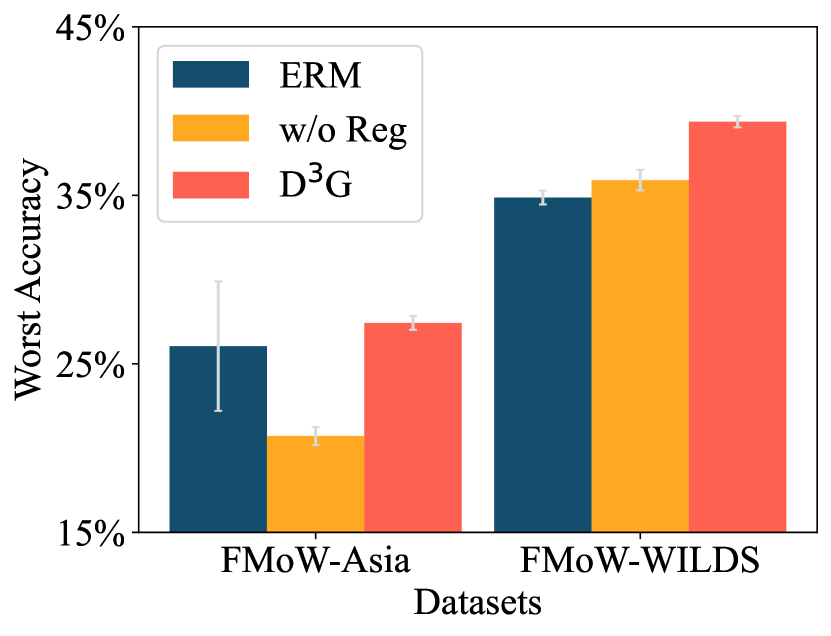
(a) FMoW

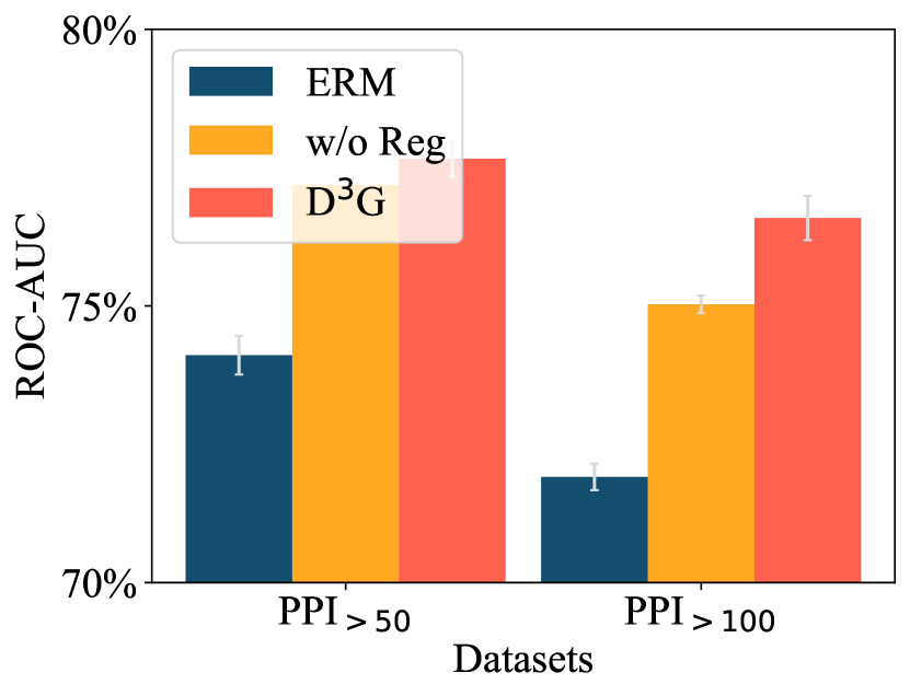
(b) ChEMBL-STRING

Figure 3: Performance comparison w.r.t. consistency regularization. Here, only fixed relations are used.

How do domain relations benefit performance? Our theoretical analysis shows that utilizing appropriate domain relations can enhance performance compared to simply averaging predictions from all domain-specific functions. To test this, we conducted empirical analysis in FMoW and ChEMBL-STRING, comparing the following variants of relations: (1) no relations used; (2) fixed relations only; (3) learned relations only; and (4) both fixed and learned relations. Our results, presented in Table 2, first indicate that using fixed relations outperforms averaging predictions, which confirms our theoretical findings and highlights the importance of using appropriate relations. However, only using learned relations resulted in a performance that is worse than using no relations at all, indicating that it is challenging to learn relations without any informative signals (such as fixed relations). Finally, combining learned relations with fixed relations results in the best performance, highlighting the importance of using learned relations to find more accurate relations for each problem.

Table 2: Comparison of using different relations. The results on FMoW and ChEMBL-STRING are reported. In this case, when no relations are used, we take the average of predictions across all domains.

Fixed	Learned	FMoW (Worst Acc. $\uparrow$)		ChEMBL-STRING (ROC-AUC $\uparrow$)
relations	relations	FMoW-Asia	FMoW-WILDS	$\text{PPI}_{>50}$	$\text{PPI}_{>100}$
		26.93 $\pm$ 0.47%	35.32 $\pm$ 0.66%	76.17 $\pm$ 0.21%	73.38 $\pm$ 0.13%
✓		27.43 $\pm$ 0.41%	39.37 $\pm$ 0.34%	77.66 $\pm$ 0.32%	76.59 $\pm$ 0.40%
	✓	21.18 $\pm$ 2.30%	36.41 $\pm$ 1.09%	77.09 $\pm$ 0.94%	75.57 $\pm$ 1.20%
✓	✓	28.12 $\pm$ 0.28%	39.47 $\pm$ 0.57%	78.67 $\pm$ 0.16%	77.24 $\pm$ 0.30%

5.4 Comparison of D³G with Domain-specific Fine-tuning

As stated in the introduction, a simple way to create a domain-specific model is by fine-tuning a generic model trained by empirical risk minimization (ERM) on reweighted training data using domain relations. In this section, we compare our proposed model D³G with this approach (referred to as RW-FT) and present the results in Table 3. We also include the performance of the strongest baseline (CORAL) for comparison. The results show that RW-FT outperforms ERM and CORAL, further confirming the effectiveness of using domain distances to improve out-of-distribution generalization. Additionally, D³G performs better than RW-FT. This may be due to the fact that using separate models for each training domain allows for more effective capture of domain-specific information.

Table 3: Comparison between D³G with domain-specific fine-tuning. Full results are presented in Appendix G.2.

Model	FMoW (Worst Acc. $\uparrow$)		ChEMBL (ROC-AUC $\uparrow$)
	FMoW-Asia	FMoW-WILDS	$\text{PPI}_{>50}$	$\text{PPI}_{>100}$
ERM	26.05%	34.87%	74.11%	71.91%
CORAL	25.87%	36.53%	75.42%	73.10%
RW-FT	27.03%	36.39%	76.31%	74.30%
D3G	28.12%	39.47%	78.67%	77.24%

5.5 Analysis of Relation Refinement

In this section, we conduct a qualitative analysis to determine if the relations learned can reflect application-specific information and improve the fixed relations extracted from domain meta-data. Specifically, we select three countries - Turkey, Syria, and Saudi Arabia from FMoW-Asia and visualize the fixed relations and learned relations among them in Figure 4. Additionally, we visualize one multi-unit residential area from each of the three countries. We observe that although Turkey is geographically close to other two countries in the Middle East (as shown by the fixed relations), its architecture style is influenced by Europe. Therefore, the learned relations refine the fixed relations and weaken the distances between Turkey and Saudi Arabia and Syria.

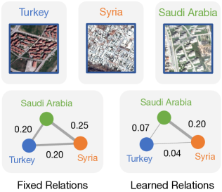
Figure 4: Analysis of relation learning. Top figures show the multi-unit residential areas of Turkey, Syria, and Saudi Arabia. Bottom figures illustrate both fixed relations and learned relations.

6 Related Work

In this section, we discuss the related work from the following two categories: out-of-distribution generalization and ensemble learning.

Out-of-distribution Generalization. To improve out-of-distribution generalization, the first line of works aligns representations across domains to learn invariant representations by (1) minimizing the divergence of feature distributions with different distance metrics (Long et al., 2015; Tzeng et al., 2014; Ganin et al., 2016b; Li et al., 2018a); (2) generating more domains and enhancing the consistency among representations (Shu et al., 2021; Wang et al., 2020; Xu et al., 2020; Yan et al., 2020; Yue et al., 2019; Zhou et al., 2020). Another line of works aims to find a predictor that is invariant across domains by imposing an explicit regularizer (Arjovsky et al., 2019; Ahuja et al., 2021a; Guo et al., 2021; Khezeli et al., 2021; Koyama & Yamaguchi, 2020; Krueger et al., 2021a; Koyama & Yamaguchi, 2020) or selectively augmenting more examples (Yao et al., 2022a, b; Gao et al., ). Unlike prior approaches that learn a single model that is domain invariant, D³G specializes the model to every given domain, which can capture more accurate information of that domain to some extend.

Ensemble methods. Our approach is closely related to ensemble methods, such as those that aggregate the predictions of multiple learners (Hansen & Salamon, 1990; Dietterich, 2000; Lakshminarayanan et al., 2017) or selectively combine the prediction from multiple experts (Jordan & Jacobs, 1994; Eigen et al., 2013; Shazeer et al., 2017; Dauphin et al., 2017). When distribution shift occurs, prior works have attempted to solve the underspecification problem by learning a diverse set of functions with the help of unlabeled data (Teney et al., 2021; Pagliardini et al., 2022; Lee et al., 2022). These methods aim to resolve the underspecification problem in the training data and disambiguate the model, thereby improving out-of-distribution robustness. Unlike prior works that rely on ensemble models to address the underspecification problem and improve out-of-distribution robustness, our proposed D³G takes a conceptually different approach by constructing domain-specific models.

7 Conclusion

In summary, the paper presents a novel method called D³G for tackling the issue of domain shifts in real-world machine learning scenarios. The approach leverages the connections between different domains to enhance the model’s robustness and employs a domain-relationship aware weighting system for each test domain. We evaluate the effectiveness of D³G on various datasets and observe that it consistently surpasses current methods, resulting in substantial performance enhancements.

Appendix A Detailed Proofs

A.1 Proof of Theorem 4.1

To prove theorem 4.1, let us first define an intermediate function

$$h_{im}^{(t)}=\frac{\sum_{i=1}^{N^{tr}}w_{it}h^{(i)}}{\sum_{k=1}^{N^{tr}}w_{kt}}$$ (14)

We then define the event $E_{n}=\{\sum_{i=1}^{N^{tr}}w_{it}>0\}$. Based on our assumption $\mathbb{E}[(\hat{h}^{(d)}(e(x))-h^{(d)}(e(x)))^{2}]=O(\frac{C(\mathcal{H})}{n_{d}})$ and $n_{d}\gtrsim n$ for each domain $d$. On the event $E_{n}$, we have that

$$\begin{split}\mathbb{E}[(h_{im}^{(t)}(e(x))-\hat{h}^{(t)}(e(x)))^{2}]\leq&\frac{\sum_{i=1}^{N^{tr}}w_{it}\cdot\mathbb{E}\left[(\hat{h}^{(i)}(e(x))-h^{(i)}(e(x)))^{2}\right]}{(\sum_{k=1}^{N^{tr}}w_{kt})^{2}}\\ \leq&\frac{\max_{i}\mathbb{E}\left[(\hat{h}^{(i)}(e(x))-h^{(i)}(e(x)))^{2}\right]}{\sum_{k=1}^{N^{tr}}w_{kt}}\\ =&O\left(\frac{C(\mathcal{H})}{n\sum_{k=1}^{N^{tr}}w_{kt}}\right),\end{split}$$ (15)

Moreover, since $\|h^{(i)}-h^{(j)}\|_{\infty}\leq G\cdot a_{ij}\leq G\cdot\|Z^{(i)}-Z^{(j)}\|\leq G\cdot B$ when $\|Z^{(i)}-Z^{(j)}\|\leq B$, we have that on the scenario $E_{n}$,

$$\left|h_{im}^{(t)}-h^{(t)}\right|=\left|\frac{\sum_{i=1}^{N^{tr}}w_{it}(h^{(i)}-h^{(t)})}{\sum_{k=1}^{N^{tr}}w_{kt}}\right|=\left|\frac{\sum_{i=1}^{N^{tr}}\mathbbm{1}\{a_{it}<B\}(h^{(i)}-h^{(t)})}{\sum_{k=1}^{N^{tr}}\mathbbm{1}\{a_{kt}<B\}}\right|\leq G\cdot B.$$ (16)

On the other hand, on the complement event $E_{n}^{c}$, as the denominator equals to 0 by our definition, we have $h_{im}^{(t)}(e(x))=0$ and therefore

$$\left|h_{im}^{(t)}(e(x))-h^{(t)}(e(x))\right|^{2}=(h^{(t)})^{2}(e(x)).$$ (17)

Consequently, we have

$$\left|h_{im}^{(t)}(e(x))-h^{(t)}(e(x))\right|^{2}\leq G^{2}B^{2}+(h^{(t)})^{2}(e(x))\cdot\mathbbm{1}_{E_{n}^{c}}.$$ (18)

Therefore,

$$\mathbb{E}\left[(\hat{h}^{(t)}-h^{(t)})^{2}\right]\lesssim\mathbb{E}\left[\frac{C(\mathcal{H})}{n\sum_{k=1}^{N^{tr}}w_{kt}}\cdot\mathbbm{1}_{E_{n}}\right]+B^{2}+\mathbb{E}\left[(h^{(t)})^{2}(e(x))\cdot\mathbbm{1}_{E_{n}^{c}}\right].$$

To bound the first term, we let $S=\sum_{i=1}^{N^{tr}}w_{it}=\sum_{i=1}^{N^{tr}}\mathbbm{1}\{\|Z^{(t)}-Z^{(i)}\|<B\}$. Since $Z^{(d)}$ are uniformly distributed on $[0,1]^{r}$, we have that $S\sim Binomial(N^{tr},q)$ with $q=\mathbb{P}(\|Z-Z^{(t)}\|<B)$. Using the property of binomial distribution, we have

$$\mathbb{E}\left[\frac{\mathbbm{1}\{S>0\}}{S}\right]\lesssim\frac{1}{N^{tr}q}\lesssim\frac{1}{N^{tr}B^{r}}.$$ (19)

Therefore the first term

$$\mathbb{E}\left[\frac{C(\mathcal{H})}{n\sum_{k=1}^{N^{tr}}w_{kt}}\cdot\mathbbm{1}_{E_{n}}\right]\lesssim\frac{C(\mathcal{H})}{nN^{tr}B^{r}}.$$ (20)

The third term can be bounded as

$$\mathbb{E}\left[(h^{(t)})^{2}(e(x))\cdot\mathbbm{1}_{E_{n}^{c}}\right]\leq\sup(h^{(t)})^{2}(e(x))\mathbb{E}[(1-q)^{N^{tr}}]\lesssim\sup(h^{(t)})^{2}(e(x))\frac{1}{N^{tr}q}\lesssim\frac{1}{N^{tr}B^{r}}.$$ (21)

Combining all the pieces, we get

$$\mathbb{E}\left[(\hat{h}^{(t)}-h^{(t)})^{2}\right]\lesssim B^{2}+\frac{C(\mathcal{H})/n}{N^{tr}B^{r}}.$$ (22)

Therefore, when $l$ is Lipshictz with respect to the first argument, we have that

$$\mathbb{E}_{(x,y)\sim P_{t}}[\ell(\hat{f}^{(t)}(x),y)]-\mathbb{E}_{(x,y)\sim P_{t}}[\ell(f^{(t)}(x),y)]\leq\mathbb{E}\left[|\hat{h}^{(t)}-h^{(t)}|\right]\leq\sqrt{\mathbb{E}[(\hat{h}^{(t)}-h^{(t)})^{2}]}\lesssim B+\sqrt{\frac{C(\mathcal{H})/n}{N^{tr}B^{r}}}.$$ (23)

If we further take $B\asymp(\frac{C(\mathcal{H})/n}{N^{tr}})^{\frac{1}{r+2}}$, we then have

$$\mathbb{E}_{(x,y)\sim P_{t}}[\ell(\hat{f}^{(t)}(x),y)]-\mathbb{E}_{(x,y)\sim P_{t}}[\ell(f^{(t)}(x),y)]\lesssim\left(\frac{C(\mathcal{H})/n}{N^{tr}}\right)^{\frac{1}{r+2}}.$$ (24)

A.2 Proof of Proposition 4.2

If we treat all training domains are equally important, i.e., $a_{it}=0$ for all $i$ and $t$, we have that

$$\hat{h}^{(t)}=\frac{\sum_{i=1}^{N^{tr}}w_{it}\hat{h}^{(i)}}{\sum_{k=1}^{N^{tr}}w_{kt}}=\frac{1}{N^{tr}}\sum_{i=1}^{N^{tr}}\hat{h}^{(i)}.$$ (25)

As it is simply the average of predictive values, we denote it by $\hat{h}^{(avg)}$.

In order to show that such an estimator performs worse than $\hat{h}$ in the minimax sense, all we need is to find an $h\in\mathcal{H}$ so that $R_{h}(h^{(avg)}(f(x)))=\Omega(1)$ even for $N,n\to\infty$.

We simply let $d\sim U[0,1]$, $e(x)\in\mathcal{N}(0,1)$ and $h^{(d)}(e(x))=d\cdot e(x)$. Under such a setting, we have that

$$\hat{h}^{(avg)}=\frac{1}{2}e(x),$$

and therefore

$$\mathbb{E}[\hat{h}^{(avg)}(e(x))-h^{(d)}(e(x))^{2}]=\mathbb{E}\left[(d-\frac{1}{2})^{2}e^{2}(x))\right]=\frac{1}{12}=\Omega(1).$$ (26)

We complete the proof.

Appendix B Detailed Description of Baselines

In this work, we compare D³G to a large number of algorithms that span different learning strategies. We group them according to their categories, and provide detailed descriptions for each algorithm below.

• vanilla: ERM (Vapnik, 1999) minimizes the average empirical loss across all training data.

• distributionally robust optimization: GroupDRO (Sagawa et al., 2020) optimizes the worst-domain loss.

• invariant learning: IRM (Arjovsky et al., 2019) learns invariant predictors that perform well across different domains. IB-IRM and IB-ERM (Ahuja et al., 2021b) performs IRM and ERM respectively with the information bottleneck constraint. V-REx (Krueger et al., 2021b) proposes a penalty on the variance of training risks. DANN (Ganin et al., 2016a) employs an adversarial network to match feature distributions. CORAL (Sun & Saenko, 2016) matches the mean and covariance of feature distributions. MMD (Li et al., 2018b) matches the maximum mean discrepancy (Gretton et al., 2012) of feature distributions. CAD (Ruan et al., 2022) introduces a contrastive adversarial domain bottleneck to enforce support match using a KL divergence. SelfReg (Kim et al., 2021) utilizes the self-supervised contrastive losses to learn domain-invariant representation. Mixup (Xu et al., 2020) performs ERM on linear interpolations of examples from random pairs of domains and their labels. LISA (Yao et al., 2022a) builds upon Mixup but interpolates samples with the same label but different domains.

Appendix C Detailed Experimental Setups and Hyperparameters

In this section, we detail our model selection for all datasets, where we use the same model architectures and use the same input $(x,y,d)$ for all approaches for fair comparison, where domain meta-data is used as features. Following  (Xu et al., 2022), we adopt a two layer MLP network, and use no data augmentation for DG-15 and TPT-48. For the FMoW dataset, we fix the network architecture as the pretrained DenseNet-121 model (Huang et al., 2017) and use the same data augmentation protocol as (Koh et al., 2021b): random crop and resize to 224 × 224 pixels, and normalization using the ImageNet channel statistics. For the ChEMBL-STRING dataset, we use graph isomorphism network (GIN) (Xu et al., 2019) as the backbone network for all algorithms, and use no data augmentation. We use an additional two layer MLP network to incorperate the domain meta-data as features for all approaches.

We list the hyperparameters in Table 4 for all datasets.

Table 4: Hyperparameters for D³G on all datasets.

Hyperparameters	DG-15	TPT-48	FMoW	ChEMBL-STRING
Learning Rate	1e-5	2e-3	1e-4	1e-4
Weight Decay	5e-4	5e-4	0	0
Batch Size	10	64	32	30
Epochs	30	40	60	100
Loss Balanced Coefficient $\lambda$	0.5	0.5	0.5	0.5
Relation Combining Coefficient $\beta$	0.8	0.5	0.8	0.5

Appendix D Additional Description of Datasets

D.1 TPT-48

Following  (Xu et al., 2022), we show the fixed relations for N (24) $\rightarrow$ S (24) and E (24) $\rightarrow$ W (24) in TPT-48. For the 24 test domains in these two tasks, we further random split them into 12 validation domains and 12 test domains.

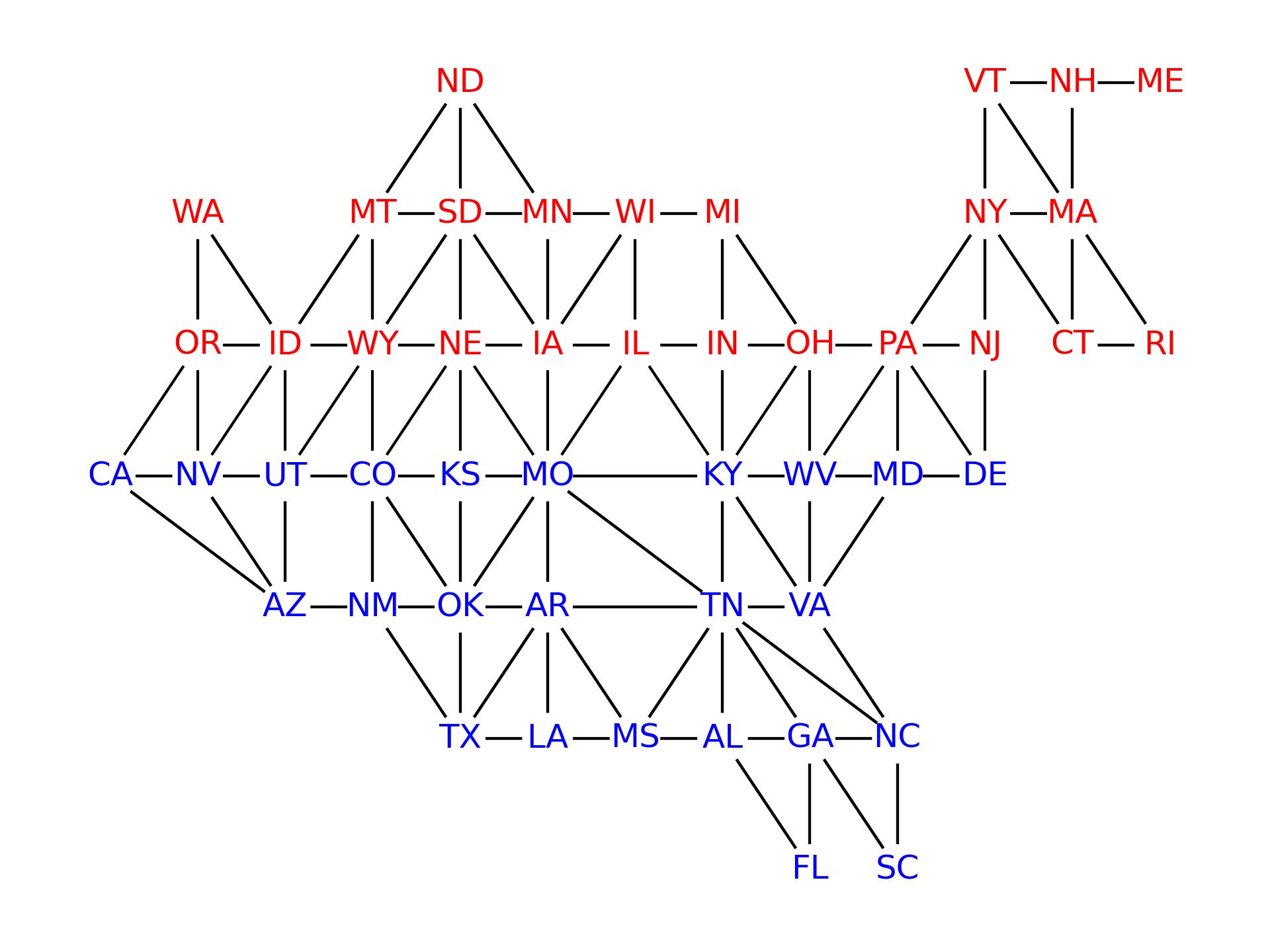
(a) N (24) $\rightarrow$ S (24)

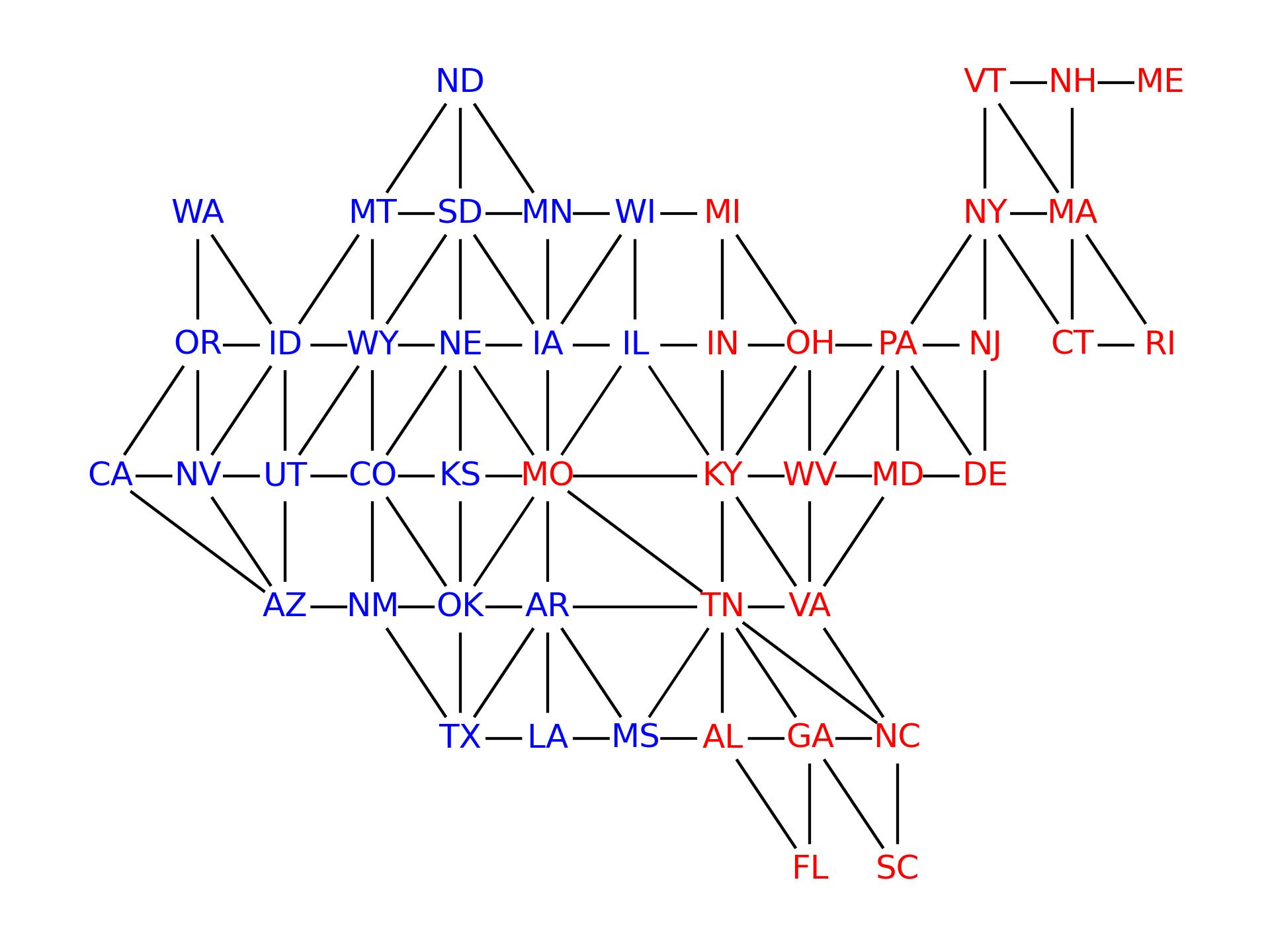
(b) E (24) $\rightarrow$ W (24)

Figure 5: Fixed relation graphs for the two tasks on TPT-48, with red nodes indicating training domains and blue nodes indicating test domains. Left: Generalization from the 24 states in the north to the 24 states in the south. Right: Generalization from the 24 states in the east to the 24 states in the west.

D.2 FMoW

For the construction of FMoW-Asia, we choose 18 countries or special administrative regions in Asia with most satellite images, and regions belong to the same sub-continent (Eastern Asia, Western Asia, Central Asia, Southern Asia and South-eastern Asia) are connected. The number of training, validation and test domains are 8, 5, 5 respectively.

D.3 ChEMBL-STRING

We follow the dataset proposed in SGNN-EBM (Liu et al., 2022), ChEMBL-STRING. It is multi-domain dataset with explicit domain relation. The three key steps are as follows:

• Filtering molecules. Among 456,331 molecules in the LSC dataset, 969 are filtered out following the pipeline in (Hu et al., 2019).

• Querying the PPI scores. Then we obtain the PPI scores by quering the ChEMBL (Mendez et al., 2018) and STRING (Szklarczyk et al., 2019) databases.

• Finally, we calculate the edge weights $w_{ij}$, i.e., domain relation score, for domain $i$ and $j$ in the domain relation graph to be $\max\{\text{PPI}(m_{i},m_{j}):m_{i}\in\mathcal{M}_{i},m_{i}\in\mathcal{M}_{j}\}$, where $\mathcal{M}_{i}$ denotes the protein set of domain $i$. The resulting domain relation graph has 1,310 nodes and 9,172 edges with non-zero weights.

The statistics of the resulting ChEMBL-STRING dataset with two thresholds can be found at Table 5.

Table 5: Statistics about $\text{PPI}_{>50}$ and $\text{PPI}_{>100}$ subsets in ChEMBL-STRING, where we use proteins as domains. Sparsity here is defined as the ratio of zero values in the domain relation graph.

Threshold	# Samples	# Proteins	Sparsity	# Train Proteins	# Valid Proteins	# Test Proteins
$\text{PPI}_{>50}$	87908	140	0.914	92	19	29
$\text{PPI}_{>100}$	58823	121	0.911	73	24	24

Appendix E Additional Results of Illustrative Toy Task

The full results on DG-15 are reported in Table 6.

Table 6: Full Results of domain shifts on DG-15. The standard deviation is computed across three seeds.

Model	ERM	GroupDRO	IRM	IB-IRM	IB-ERM	V-REx	DANN
Accuracy	44.0 $\pm$ 4.6%	47.7 $\pm$ 9.0%	43.9 $\pm$ 5.1%	45.4 $\pm$ 5.7%	43.1 $\pm$ 1.9%	44.0 $\pm$ 4.1%	43.1 $\pm$ 4.5%
Model	CORAL	MMD	CAD	SelfReg	Mixup	LISA	D3G (ours)
Accuracy	43.5 $\pm$ 1.5%	41.3 $\pm$ 1.0%	43.3 $\pm$ 2.8%	40.7 $\pm$ 0.7%	41.3 $\pm$ 3.9%	47.4 $\pm$ 0.9%	77.5 $\pm$ 2.5%

Appendix F Additional Results of Real World Domain Shifts

F.1 Full Results on FMoW

The full results on FMoW are reported in Table 7.

Table 7: Full results of domain shifts on FMoW. The standard deviation is computed across three seeds.

	FMoW-Aisa		FMoW-WILDS
	Worst Acc.	Average Acc.	Worst Acc.	Average Acc.
ERM	26.05 $\pm$ 3.84%	35.50 $\pm$ 0.20%	34.87 $\pm$ 0.41%	52.64 $\pm$ 0.30%
GroupDRO	26.24 $\pm$ 1.85%	34.14 $\pm$ 0.15%	31.16 $\pm$ 2.12%	46.79 $\pm$ 0.08%
IRM	25.02 $\pm$ 2.38%	33.28 $\pm$ 0.68%	32.54 $\pm$ 1.92%	50.39 $\pm$ 0.66%
IB-IRM	26.30 $\pm$ 1.51%	35.43 $\pm$ 0.37%	34.94 $\pm$ 1.38%	51.90 $\pm$ 0.27%
IB-ERM	26.78 $\pm$ 1.34%	35.65 $\pm$ 0.62%	35.52 $\pm$ 0.79%	52.36 $\pm$ 0.31%
V-REx	26.63 $\pm$ 0.93%	35.71 $\pm$ 0.21%	37.64 $\pm$ 0.92%	52.89 $\pm$ 0.10%
DANN	25.62 $\pm$ 1.59%	34.53 $\pm$ 0.76%	33.78 $\pm$ 1.55%	50.50 $\pm$ 0.25%
CORAL	25.87 $\pm$ 1.97%	35.43 $\pm$ 0.12%	36.53 $\pm$ 0.15%	51.89 $\pm$ 0.35%
MMD	25.06 $\pm$ 2.19%	33.77 $\pm$ 0.57%	35.48 $\pm$ 1.81%	50.17 $\pm$ 0.17%
CAD	26.13 $\pm$ 1.82%	34.97 $\pm$ 0.41%	35.17 $\pm$ 1.73%	50.92 $\pm$ 0.35%
SelfReg	24.81 $\pm$ 1.77%	36.27 $\pm$ 0.50%	37.33 $\pm$ 0.87%	51.71 $\pm$ 0.28%
Mixup	26.99 $\pm$ 1.27%	36.41 $\pm$ 0.31%	35.67 $\pm$ 0.53%	53.50 $\pm$ 0.11%
LISA	26.05 $\pm$ 2.09%	35.17 $\pm$ 0.69%	34.59 $\pm$ 1.28%	50.95 $\pm$ 0.13%
D3G (ours)	28.12 $\pm$ 0.28%	37.71 $\pm$ 0.48%	39.47 $\pm$ 0.57%	54.36 $\pm$ 0.12%

F.2 Full Results on ChEMBL-STRING

The full results on ChEMBL-STRING are reported in Table 8.

Table 8: Full results of domain shifts on ChEMBL-STRING.

	$\text{PPI}_{>50}$		$\text{PPI}_{>100}$
	ROC-AUC	Accuracy	ROC-AUC	Accuracy
ERM	74.11 $\pm$ 0.35%	71.15 $\pm$ 0.43%	71.91 $\pm$ 0.24%	70.39 $\pm$ 0.36%
GroupDRO	73.98 $\pm$ 0.25%	69.59 $\pm$ 0.56%	71.55 $\pm$ 0.59%	67.00 $\pm$ 0.85%
IRM	52.71 $\pm$ 0.50%	64.30 $\pm$ 0.02%	51.73 $\pm$ 1.54%	63.16 $\pm$ 1.82%
IB-IRM	52.12 $\pm$ 0.91%	63.57 $\pm$ 0.21%	52.33 $\pm$ 1.06%	63.39 $\pm$ 1.35%
IB-ERM	74.69 $\pm$ 0.14%	71.47 $\pm$ 0.43%	73.32 $\pm$ 0.21%	71.18 $\pm$ 0.27%
V-REx	71.46 $\pm$ 1.47%	71.33 $\pm$ 0.90%	69.37 $\pm$ 0.85%	70.93 $\pm$ 1.06%
DANN	73.49 $\pm$ 0.45%	70.74 $\pm$ 0.38%	72.22 $\pm$ 0.10%	70.41 $\pm$ 0.25%
CORAL	75.42 $\pm$ 0.15%	71.71 $\pm$ 0.34%	73.10 $\pm$ 0.14%	70.88 $\pm$ 0.10%
MMD	75.11 $\pm$ 0.27%	71.57 $\pm$ 0.40%	73.30 $\pm$ 0.50%	71.15 $\pm$ 0.63%
CAD	75.17 $\pm$ 0.64%	71.97 $\pm$ 0.83%	72.92 $\pm$ 0.39%	71.34 $\pm$ 0.46%
SelfReg	75.42 $\pm$ 0.42%	70.34 $\pm$ 0.57%	72.63 $\pm$ 0.71%	69.14 $\pm$ 0.90%
Mixup	74.40 $\pm$ 0.54%	71.39 $\pm$ 0.29%	71.31 $\pm$ 1.06%	70.29 $\pm$ 0.15%
LISA	74.30 $\pm$ 0.59%	71.72 $\pm$ 0.66%	71.45 $\pm$ 0.44%	70.37 $\pm$ 0.29%
D3G (ours)	78.67 $\pm$ 0.16%	74.25 $\pm$ 0.34%	77.24 $\pm$ 0.30%	73.50 $\pm$ 0.24%

Appendix G Additional Results of Analysis

G.1 Full Results of the Analysis of Consistency Regularization

In Table 9, we report the full results of the analysis of consistency regularization with standard deviation over three seeds.

Table 9: Full results of comparison w.r.t. consistency regularization. Here, only fixed relations are used.

Model	FMoW (Worst Acc. $\uparrow$)		ChEMBL-STRING (ROC-AUC $\uparrow$)
	FMoW-Asia	FMoW-WILDS	$\text{PPI}_{>50}$	$\text{PPI}_{>100}$
ERM	26.05 $\pm$ 3.84%	34.87 $\pm$ 0.41%	74.11 $\pm$ 0.35%	71.91 $\pm$ 0.24%
w/o Regularization	20.72 $\pm$ 0.54%	35.90 $\pm$ 0.61%	77.19 $\pm$ 0.06%	75.03 $\pm$ 0.16%
D3G	27.43 $\pm$ 0.41%	39.37 $\pm$ 0.34%	77.66 $\pm$ 0.32%	76.59 $\pm$ 0.40%

G.2 Full Results of Comparison with Domain-specific Fine-tuning

In Table 10, we report the full results of comparison with domain-specific fine-tuning.

Table 10: Full results of comparison between D³G with domain-specific fine-tuning.

Model	FMoW (Worst Acc. $\uparrow$)		ChEMBL (ROC-AUC $\uparrow$)
	FMoW-Asia	FMoW-WILDS	$\text{PPI}_{>50}$	$\text{PPI}_{>100}$
ERM	26.05 $\pm$ 3.84%	34.87 $\pm$ 0.41%	74.11 $\pm$ 0.35%	71.91 $\pm$ 0.24%
CORAL	25.87 $\pm$ 1.97%	36.53 $\pm$ 0.15%	75.42 $\pm$ 0.15%	73.10 $\pm$ 0.14%
RW-FT	27.03 $\pm$ 1.03%	36.39 $\pm$ 1.28%	76.31 $\pm$ 0.35%	74.30 $\pm$ 0.40%
D3G	28.12 $\pm$ 0.28%	39.47 $\pm$ 0.57%	78.67 $\pm$ 0.16%	77.24 $\pm$ 0.30%

References

- cci (2020) Climate change in the contiguous united states. https://github.com/washingtonpost/data-2C-beyond-the-limit-usa, 2020.
- Ahuja et al. (2021a) Ahuja, K., Caballero, E., Zhang, D., Bengio, Y., Mitliagkas, I., and Rish, I. Invariance principle meets information bottleneck for out-of-distribution generalization. In NeurIPS, 2021a.
- Ahuja et al. (2021b) Ahuja, K., Caballero, E., Zhang, D., Bengio, Y., Mitliagkas, I., and Rish, I. Invariance principle meets information bottleneck for out-of-distribution generalization. 2021b.
- Arjovsky et al. (2019) Arjovsky, M., Bottou, L., Gulrajani, I., and Lopez-Paz, D. Invariant risk minimization. arXiv preprint arXiv:1907.02893, 2019.
- Chen et al. (2020) Chen, Y., Wu, L., and Zaki, M. J. Iterative deep graph learning for graph neural networks: Better and robust node embeddings. ArXiv, abs/2006.13009, 2020.
- Dauphin et al. (2017) Dauphin, Y. N., Fan, A., Auli, M., and Grangier, D. Language modeling with gated convolutional networks. In International conference on machine learning, pp. 933–941. PMLR, 2017.
- Dietterich (2000) Dietterich, T. G. Ensemble methods in machine learning. In International workshop on multiple classifier systems, pp. 1–15. Springer, 2000.
- Eigen et al. (2013) Eigen, D., Ranzato, M., and Sutskever, I. Learning factored representations in a deep mixture of experts. arXiv preprint arXiv:1312.4314, 2013.
- Ganin et al. (2016a) Ganin, Y., Ustinova, E., Ajakan, H., Germain, P., Larochelle, H., Laviolette, F., Marchand, M., and Lempitsky, V. Domain-adversarial training of neural networks. The journal of machine learning research, 17(1):2096–2030, 2016a.
- Ganin et al. (2016b) Ganin, Y., Ustinova, E., Ajakan, H., Germain, P., Larochelle, H., Laviolette, F., Marchand, M., and Lempitsky, V. S. Domain-adversarial training of neural networks. In J. Mach. Learn. Res., 2016b.
- (11) Gao, I., Sagawa, S., Koh, P. W., Hashimoto, T., and Liang, P. Out-of-distribution robustness via targeted augmentations. In NeurIPS 2022 Workshop on Distribution Shifts: Connecting Methods and Applications.
- Gretton et al. (2012) Gretton, A., Borgwardt, K. M., Rasch, M. J., Schölkopf, B., and Smola, A. A kernel two-sample test. Journal of Machine Learning Research, 13(25):723–773, 2012. URL http://jmlr.org/papers/v13/gretton12a.html.
- Gulrajani & Lopez-Paz (2021) Gulrajani, I. and Lopez-Paz, D. In search of lost domain generalization. ArXiv, abs/2007.01434, 2021.
- Guo et al. (2021) Guo, R., Zhang, P., Liu, H., and Kıcıman, E. Out-of-distribution prediction with invariant risk minimization: The limitation and an effective fix. ArXiv, abs/2101.07732, 2021.
- Hansen & Salamon (1990) Hansen, L. K. and Salamon, P. Neural network ensembles. IEEE transactions on pattern analysis and machine intelligence, 12(10):993–1001, 1990.
- Hu et al. (2019) Hu, W., Liu, B., Gomes, J., Zitnik, M., Liang, P., Pande, V., and Leskovec, J. Strategies for pre-training graph neural networks. arXiv preprint arXiv:1905.12265, 2019.
- Huang et al. (2017) Huang, G., Liu, Z., Van Der Maaten, L., and Weinberger, K. Q. Densely connected convolutional networks. In Proceedings of the IEEE conference on computer vision and pattern recognition, pp. 4700–4708, 2017.
- Ji et al. (2022) Ji, Y., Zhang, L., Wu, J., Wu, B., Huang, L.-K., Xu, T., Rong, Y., Li, L., Ren, J., Xue, D., Lai, H., Xu, S., Feng, J., Liu, W., Luo, P., Zhou, S., Huang, J., Zhao, P., and Bian, Y. Drugood: Out-of-distribution (ood) dataset curator and benchmark for ai-aided drug discovery - a focus on affinity prediction problems with noise annotations. ArXiv, abs/2201.09637, 2022.
- Jordan & Jacobs (1994) Jordan, M. I. and Jacobs, R. A. Hierarchical mixtures of experts and the em algorithm. Neural computation, 6(2):181–214, 1994.
- Khezeli et al. (2021) Khezeli, K., Blaas, A., Soboczenski, F., Chia, N. K. K., and Kalantari, J. On invariance penalties for risk minimization. ArXiv, abs/2106.09777, 2021.
- Kim et al. (2021) Kim, D., Yoo, Y., Park, S., Kim, J., and Lee, J. Selfreg: Self-supervised contrastive regularization for domain generalization. In Proceedings of the IEEE/CVF International Conference on Computer Vision, pp. 9619–9628, 2021.
- Koh et al. (2021a) Koh, P. W., Sagawa, S., Marklund, H., Xie, S. M., Zhang, M., Balsubramani, A., Hu, W., Yasunaga, M., Phillips, R. L., Beery, S., Leskovec, J., Kundaje, A., Pierson, E., Levine, S., Finn, C., and Liang, P. Wilds: A benchmark of in-the-wild distribution shifts. In ICML, 2021a.
- Koh et al. (2021b) Koh, P. W., Sagawa, S., Xie, S. M., Zhang, M., Balsubramani, A., Hu, W., Yasunaga, M., Phillips, R. L., Gao, I., Lee, T., et al. Wilds: A benchmark of in-the-wild distribution shifts. In International Conference on Machine Learning, pp. 5637–5664. PMLR, 2021b.
- Koyama & Yamaguchi (2020) Koyama, M. and Yamaguchi, S. Out-of-distribution generalization with maximal invariant predictor. ArXiv, abs/2008.01883, 2020.
- Krueger et al. (2021a) Krueger, D., Caballero, E., Jacobsen, J.-H., Zhang, A., Binas, J., Priol, R. L., and Courville, A. C. Out-of-distribution generalization via risk extrapolation (rex). In ICML, 2021a.
- Krueger et al. (2021b) Krueger, D., Caballero, E., Jacobsen, J.-H., Zhang, A., Binas, J., Zhang, D., Le Priol, R., and Courville, A. Out-of-distribution generalization via risk extrapolation (rex). In International Conference on Machine Learning, pp. 5815–5826. PMLR, 2021b.
- Lakshminarayanan et al. (2017) Lakshminarayanan, B., Pritzel, A., and Blundell, C. Simple and scalable predictive uncertainty estimation using deep ensembles. Conference on Neural Information Processing Systems, 2017.
- Lee et al. (2022) Lee, Y., Yao, H., and Finn, C. Diversify and disambiguate: Learning from underspecified data. arXiv preprint arXiv:2202.03418, 2022.
- Li et al. (2018a) Li, H., Pan, S. J., Wang, S., and Kot, A. C. Domain generalization with adversarial feature learning. 2018 IEEE/CVF Conference on Computer Vision and Pattern Recognition, pp. 5400–5409, 2018a.
- Li et al. (2018b) Li, H., Pan, S. J., Wang, S., and Kot, A. C. Domain generalization with adversarial feature learning. In Proceedings of the IEEE conference on computer vision and pattern recognition, pp. 5400–5409, 2018b.
- Liu et al. (2022) Liu, S., Qu, M., Zhang, Z., Cai, H., and Tang, J. Structured multi-task learning for molecular property prediction. In International Conference on Artificial Intelligence and Statistics, pp. 8906–8920. PMLR, 2022.
- Long et al. (2015) Long, M., Cao, Y., Wang, J., and Jordan, M. I. Learning transferable features with deep adaptation networks. ArXiv, abs/1502.02791, 2015.
- Mendez et al. (2018) Mendez, D., Gaulton, A., Bento, A. P., Chambers, J., De Veij, M., Félix, E., Magariños, M., Mosquera, J., Mutowo, P., Nowotka, M., Gordillo-Marañón, M., Hunter, F., Junco, L., Mugumbate, G., Rodriguez-Lopez, M., Atkinson, F., Bosc, N., Radoux, C., Segura-Cabrera, A., Hersey, A., and Leach, A. ChEMBL: towards direct deposition of bioassay data. Nucleic Acids Research, 47(D1):D930–D940, 11 2018. ISSN 0305-1048. doi: 10.1093/nar/gky1075. URL https://doi.org/10.1093/nar/gky1075.
- Pagliardini et al. (2022) Pagliardini, M., Jaggi, M., Fleuret, F., and Karimireddy, S. P. Agree to disagree: Diversity through disagreement for better transferability. arXiv preprint arXiv:2202.04414, 2022.
- Ruan et al. (2022) Ruan, Y., Dubois, Y., and Maddison, C. J. Optimal representations for covariate shift. 2022.
- Sagawa et al. (2020) Sagawa, S., Koh, P. W., Hashimoto, T. B., and Liang, P. Distributionally robust neural networks for group shifts: On the importance of regularization for worst-case generalization. International Conference on Learning Representations, 2020.
- Shazeer et al. (2017) Shazeer, N., Mirhoseini, A., Maziarz, K., Davis, A., Le, Q., Hinton, G., and Dean, J. Outrageously large neural networks: The sparsely-gated mixture-of-experts layer. arXiv preprint arXiv:1701.06538, 2017.
- Shu et al. (2021) Shu, Y., Cao, Z., Wang, C., Wang, J., and Long, M. Open domain generalization with domain-augmented meta-learning. 2021 IEEE/CVF Conference on Computer Vision and Pattern Recognition (CVPR), pp. 9619–9628, 2021.
- Sun & Saenko (2016) Sun, B. and Saenko, K. Deep coral: Correlation alignment for deep domain adaptation. In European conference on computer vision, pp. 443–450. Springer, 2016.
- Szklarczyk et al. (2019) Szklarczyk, D., Gable, A. L., Lyon, D., Junge, A., Wyder, S., Huerta-Cepas, J., Simonovic, M., Doncheva, N. T., Morris, J. H., Bork, P., et al. String v11: protein–protein association networks with increased coverage, supporting functional discovery in genome-wide experimental datasets. Nucleic acids research, 47(D1):D607–D613, 2019.
- Teney et al. (2021) Teney, D., Abbasnejad, E., Lucey, S., and Hengel, A. v. d. Evading the simplicity bias: Training a diverse set of models discovers solutions with superior ood generalization. arXiv preprint arXiv:2105.05612, 2021.
- Tzeng et al. (2014) Tzeng, E., Hoffman, J., Zhang, N., Saenko, K., and Darrell, T. Deep domain confusion: Maximizing for domain invariance. ArXiv, abs/1412.3474, 2014.
- Vapnik (1999) Vapnik, V. N. An overview of statistical learning theory. IEEE transactions on neural networks, 10 5:988–99, 1999.
- Vose et al. (2014) Vose, R. S., Applequist, S., Squires, M., Durre, I., Menne, M. J., Williams, C. N. J., Fenimore, C., Gleason, K., and Arndt, D. Gridded 5km ghcn-daily temperature and precipitation dataset (nclimgrid) version 1. Maximum Temperature, Minimum Temperature, Average Temperature, and Precipitation, 2014.
- Wang et al. (2020) Wang, Y., Li, H., and Kot, A. C. Heterogeneous domain generalization via domain mixup. ICASSP 2020 - 2020 IEEE International Conference on Acoustics, Speech and Signal Processing (ICASSP), pp. 3622–3626, 2020.
- Xu et al. (2019) Xu, K., Hu, W., Leskovec, J., and Jegelka, S. How powerful are graph neural networks? In International Conference on Learning Representations, 2019. URL https://openreview.net/forum?id=ryGs6iA5Km.
- Xu et al. (2020) Xu, M., Zhang, J., Ni, B., Li, T., Wang, C., Tian, Q., and Zhang, W. Adversarial domain adaptation with domain mixup. In AAAI, 2020.
- Xu et al. (2022) Xu, Z., He, H., Lee, G.-H., Wang, Y., and Wang, H. Graph-relational domain adaptation. arXiv preprint:2202.03628, 2022.
- Yan et al. (2020) Yan, S., Song, H., Li, N., Zou, L., and Ren, L. Improve unsupervised domain adaptation with mixup training. ArXiv, abs/2001.00677, 2020.
- Yao et al. (2022a) Yao, H., Wang, Y., Li, S., Zhang, L., Liang, W., Zou, J., and Finn, C. Improving out-of-distribution robustness via selective augmentation. arXiv preprint arXiv:2201.00299, 2022a.
- Yao et al. (2022b) Yao, H., Wang, Y., Zhang, L., Zou, J., and Finn, C. C-mixup: Improving generalization in regression. arXiv preprint arXiv:2210.05775, 2022b.
- Yue et al. (2019) Yue, X., Zhang, Y., Zhao, S., Sangiovanni-Vincentelli, A. L., Keutzer, K., and Gong, B. Domain randomization and pyramid consistency: Simulation-to-real generalization without accessing target domain data. 2019 IEEE/CVF International Conference on Computer Vision (ICCV), pp. 2100–2110, 2019.
- Zhou et al. (2020) Zhou, K., Yang, Y., Hospedales, T. M., and Xiang, T. Deep domain-adversarial image generation for domain generalisation. ArXiv, abs/2003.06054, 2020.