Toward Large Kernel Models

Abstract

Recent studies indicate that kernel machines can often perform similarly or better than deep neural networks (DNNs) on small datasets. The interest in kernel machines has been additionally bolstered by the discovery of their equivalence to wide neural networks in certain regimes. However, a key feature of DNNs is their ability to scale the model size and training data size independently, whereas in traditional kernel machines model size is tied to data size. Because of this coupling, scaling kernel machines to large data has been computationally challenging. In this paper, we provide a way forward for constructing large-scale general kernel models, which are a generalization of kernel machines that decouples the model and data, allowing training on large datasets. Specifically, we introduce EigenPro 3.0, an algorithm based on projected dual preconditioned SGD and show scaling to model and data sizes which have not been possible with existing kernel methods. We provide a PyTorch based implementation which can take advantage of multiple GPUs.

1 Introduction

Deep neural networks (DNNs) have become the gold standard for many large-scale machine learning tasks. Two key factors that contribute to the success of DNNs are the large model sizes and the large number of training samples. Quoting from (Kaplan et al., 2020) “performance depends most strongly on scale, which consists of three factors: the number of model parameters $N$ (excluding embeddings), the size of the dataset $D$, and the amount of compute $C$ used for training. Within reasonable limits, performance depends very weakly on other architectural hyperparameters such as depth vs. width”. Major community effort and great amount of resources have been invested in scaling models and data size, as well as in understanding the relationship between the number of model parameters, compute, data size, and performance. Many current architectures have hundreds of billions of parameters and are trained on large datasets with nearly a trillion data points (e.g., Table 1 in (Hoffmann et al., 2022)). Scaling both model size and the number of training samples are seen as crucial for optimal performance.

Recently, there has been a surge in research on the equivalence of special cases of DNNs and kernel machines. For instance, the Neural Tangent Kernel (NTK) has been used to understand the behavior of fully-connected DNNs in the infinite width limit by using a fixed kernel (Jacot et al., 2018). A rather general version of that phenomenon was shown in (Zhu et al., 2022). Similarly, the Convolutional Neural Tangent Kernel (CNTK) (Li et al., 2019) is the NTK for convolutional neural networks, and has been shown to achieve accuracy comparable to AlexNet (Krizhevsky et al., 2012) on the CIFAR10 dataset.

These developments have sparked interest in the potential of kernel machines as an alternative for DNNs. Kernel machines are relatively well-understood theoretically, are stable, somewhat interpretable, and have been shown to perform similarly to DNNs on small datasets (Arora et al., 2020; Lee et al., 2020; Radhakrishnan et al., 2022b), particularly on tabular data (Geifman et al., 2020; Radhakrishnan et al., 2022a). However, in order for kernels to be a viable alternative to DNNs, it is necessary to develop methods to scale kernel machines to large datasets.

The problem of scaling. Similarly to DNN, to achieve optimal performance of kernel models, it is not sufficient to just increase the size of the training set for a fixed model size, but the model size must scale as well. Fig. 1 illustrates this property on a small-scale example (see Appendix LABEL:sec:fig1_app for the details). The figure demonstrates that the best performance cannot be achieved solely by increasing the dataset size. Once the model reaches its capacity, adding more data leads to marginal, if any, performance improvements. On the other hand, we see that the saturation point for each model is not achieved until the number of samples significantly exceeds the model size. This illustration highlights the need for algorithms that can independently scale dataset size and model size for optimal performance.

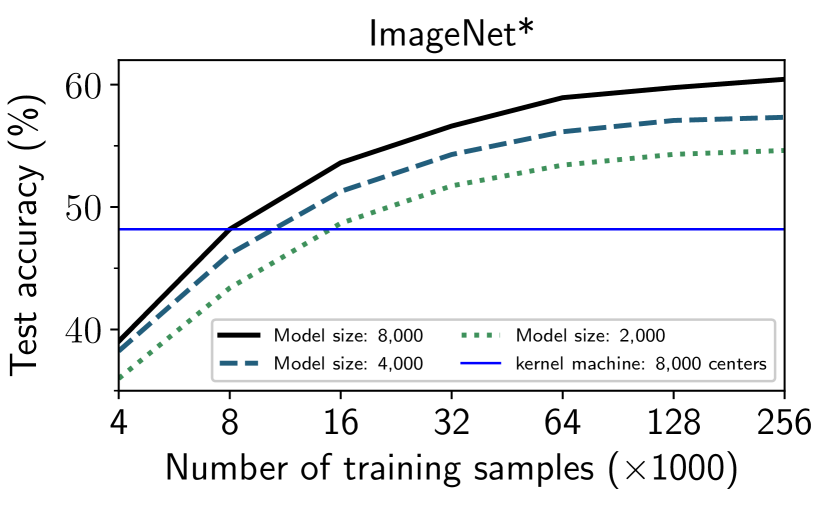
Figure 1: Increasing number of training samples for a fixed model size is helpful but insufficient for optimal performance. The model size must scale as well. See Appendix LABEL:sec:fig1_app for details.

1.1 Main contributions

We introduce EigenPro 3.0 for learning general kernel models that can handle large model sizes. In our numerical experiments, we train models with up to $1$ million centers on $5$ million samples. To the best of our knowledge, this was not achievable with any other existing method. Our work provides a path forward to scaling both the model size and size of the training dataset, independently.

1.2 Prior work

A naive approach for training kernel machines is to directly solve the equivalent kernel matrix inversion problem. In general, the computational complexity of solving the kernel matrix inversion problem is $O(n^{3})$, where $n$ is the number of training samples. Thus, computational cost grows rapidly with the size of the dataset, making it computationally intractable for datasets with more than $\sim 10^{5}$ data points.

A number of methods have been proposed to tackle this issue by utilizing various iterative algorithms and approximations. We provide a brief overview of the key ideas below.

Gradient Descent(GD) based algorithms: Gradient descent (GD) based methods, such as Pegasos (Shalev-Shwartz et al., 2007), have a more manageable computational complexity of $O(n^{2})$ and can be used in a stochastic setting, allowing for more efficient implementation. Preconditioned stochastic gradient descent based method, EigenPro (Ma & Belkin, 2017) was introduced to accelerate convergence of Pegasos. EigenPro is an iterative algorithm for kernel machines that uses a preconditioned Richardson iteration (Richardson, 1911). Its performance was further improved in EigenPro 2.0 (Ma & Belkin, 2019) by reducing the computational and memory costs for the preconditioner through the use of a Nyström extension (Williams & Seeger, 2000) and introducing full hardware (GPU) utilization by adaptively auto-tuning the learning rate.

However, Kernel machines are limited in scalability due to the coupling between the model and the training set. With modern hardware, these methods can handle just above one million training data points. A more in-depth discussion about EigenPro can be found in Section 2.1.

Large scale Nyström-approximate models: Nyström methods have been a popular strategy for applying kernel machines at scale starting with (Williams & Seeger, 2000). We refer the reader to Section 2 for a detailed description of the Nyström approximation. Methods such as Nytro (Camoriano et al., 2016) and Falkon (Rudi et al., 2017) use Nyström approximation (NA) in combination with other techniques to improve performance. Specifically, Nytro combines NA with gradient descent to improve the condition number, while Falkon uses NA in combination with the Conjugate Gradient method. While these methods allow for very large training sets, they are limited in terms of the model size due to memory limitations. For example, the largest models considered (Meanti et al., 2020) have about $100,\!000$ centers. With $340$GB RAM available to us on the Expanse cluster (Towns et al., 2014), we were able to run Falkon  with at $256,\!000$ model size (Figure 5). However, scaling to $512,\!000$ model size, already requires over $1$TB RAM which goes beyond specifications of most current high end servers.

Sparse Gaussian Process: Methods from the literature on Gaussian Processes, e.g. (Titsias, 2009), use so-called inducing points to control the model complexity. While several follow-ups such as (Wilson & Nickisch, 2015) and Gpytorch  (Gardner et al., 2018), and GPFlow (Matthews et al., 2017) have been applied in practice, they require quadratic memory in terms of the number of the inducing points, thus preventing scaling to large models. A closely related concept is that of kernel herding (Chen et al., 2010). The focus of these methods is largely on selecting “good” model centers, rather than scaling-up the training procedure. Our work is complementary to that line of research.

Random Fourier Features (RFFs): RFF is a popular method first introduced in (Rahimi & Recht, 2007) to approximate kernel machines using so-called “Random Fourier Features”. However, it is generally believed that Nyström methods outperform RFF  (Yang et al., 2012).

2 Preliminaries and Background

Kernel Machines: Kernel machines, (Schölkopf et al., 2002) are non-parametric predictive models. Given training data $(X,\bm{y})=\left\{\bm{x}_{i}\in\mathbb{R}^{d},y_{i}\in\mathbb{R}\right\}_{i=1}^{n}$ a kernel machine is a model of the form

$$f(\bm{x})=\sum_{i=1}^{n}\alpha_{i}K(\bm{x},\bm{x}_{i}).$$ (1)

Here, $K:\mathbb{R}^{d}\times\mathbb{R}^{d}\rightarrow\mathbb{R}$ is a positive semi-definite symmetric kernel function (Aronszajn, 1950). According to the representer theorem (Kimeldorf & Wahba, 1970), the unique solution to the infinite-dimensional optimization problem

$$\arg~{}\underset{f\in{\bm{\mathcal{H}}}}{\rm min}~{}\,\sum_{i=1}^{n}(f(\bm{x}_{i})-y_{i})^{2}+\lambda\left\|f\right\|_{\bm{\mathcal{H}}}^{2}$$ (2)

has the form given in Eq. 1.

Here ${\bm{\mathcal{H}}}$ is the (unique) reproducing kernel Hilbert space (RKHS) corresponding to $K$.

It can be seen that $\bm{\alpha}=(\alpha_{1},\ldots,\alpha_{n})$ in equation 1 is the unique solution to the linear system,

$$(K(X,X)+\lambda I_{n})\bm{\alpha}=\bm{y}.$$ (3)

General kernel models are models of the form,

$$f(\bm{x})=\sum_{i=1}^{p}\alpha_{i}K(\bm{x},\mathbf{z}_{i}),$$

where $Z=\{z_{i}\in\mathbb{R}^{d}\}_{i=1}^{p}$ is the set of centers, which is not necessary the same as the training set. We will refer to $p$ as the model size. Note that kernel machines are a special type of general kernel models with $Z=X$. Our goal will be to solve equation 2 with this new constraint on $f$.

Note that when $Z\subset X$, is a random subset of the training data, the resulting model is called a Nyström approximate (NA) model (Williams & Seeger, 2000).

In contrast to kernel machines, general kernel models, such as classical RBF networks (Poggio & Girosi, 1990), allow for the separation of the model and training set. General kernel models also provide explicit control over model capacity by allowing the user to choose $p$ separately from the training data size. This makes them a valuable tool for many applications, particularly when dealing with large datasets.

Notation: In what follows, functions are lowercase letters $a$, sets are uppercase letters $A$, vectors are lowercase bold letters $\bm{a}$, matrices are uppercase bold letters $\bm{A}$, operators are calligraphic letters $\mathcal{A},$ spaces and sub-spaces are boldface calligraphic letters $\bm{\mathcal{A}}.$

Evaluations and kernel matrices: The vector of evaluations of a function $f$ over a set $X=\left\{\bm{x}_{i}\right\}_{i=1}^{n}$ is denoted $f(X):=(f(\bm{x}_{i}))\in\mathbb{R}^{n}$. For sets $X$ and $Z$, with $|X|=n$ and $|Z|=p$, we denote the kernel matrix $K(X,Z)\in\mathbb{R}^{n\times p},$ while $K(Z,X)=K(X,Z)^{\top}$. Similarly, $K(\cdot,X)\in{\bm{\mathcal{H}}}^{n}$ is a vector of functions, and we use $K(\cdot,X)\bm{\alpha}:=\sum_{i=1}^{n}K(\cdot,\bm{x}_{i})\alpha_{i}\in{\bm{\mathcal{H}}},$ to denote their linear combination. Finally, for an operator $\mathcal{A},$ a function $a$, and a set $A=\{\bm{a}_{i}\}_{i=1}^{k}$, we denote the vector of evaluations of the output,

$$\mathcal{A}\left\{a\right\}(A):=(b(\bm{a}_{i}))\in\mathbb{R}^{k}\qquad\text{where}\quad b=\mathcal{A}\left(a\right).$$ (4)

Definition 1 (Top-$q$ eigensystem).

Let $\lambda_{1}>\lambda_{2}>\ldots>\lambda_{n},$ be the eigenvalues of a hermitian matrix $\bm{A}\in\mathbb{R}^{n\times n}$, i.e., for unit-norm $\bm{e}_{i}$, we have $\bm{A}\bm{e}_{i}=\lambda_{i}\bm{e}_{i}$. Then we call the tuple $(\Lambda_{q},\bm{E}_{q},\lambda_{q+1})$ the top-$q$ eigensystem, where

$$\Lambda_{q}:={\rm diag}(\lambda_{1},\lambda_{2},\ldots,\lambda_{q})\in\mathbb{R}^{q\times q},\text{ and}$$ (5)

$$\bm{E}_{q}:=[\bm{e}_{1},\bm{e}_{2},\ldots,\bm{e}_{q}]\in\mathbb{R}^{n\times q}.$$ (6)

Definition 2 (Fréchet derivative).

Given a function $J:{\bm{\mathcal{H}}}\to\mathbb{R}$, the Fréchet derivative of $J$ with respect to $f$ is a linear functional, denoted $\nabla_{f}J$, such that for $h\in{\bm{\mathcal{H}}}$

$$\lim_{\left\|h\right\|_{\bm{\mathcal{H}}}\rightarrow 0}\frac{\left|J(f+h)-J(f)-\nabla_{f}J(h)\right|}{\left\|h\right\|_{\bm{\mathcal{H}}}}=0.$$ (7)

Since $\nabla_{f}J$ is a linear functional, it lies in the dual space ${\bm{\mathcal{H}}}^{*}.$ Since ${\bm{\mathcal{H}}}$ is a Hilbert space, it is self-dual, whereby ${\bm{\mathcal{H}}}^{*}={\bm{\mathcal{H}}}.$ If $f$ is a general kernel model, and $L$ is the square loss for a given dataset $(X,\bm{y})$, i.e., $L(f):=\frac{1}{2}\sum_{i=1}^{n}(f(\bm{x}_{i})-y_{i})^{2}$ we can apply the chain rule, and using reproducing property of ${\bm{\mathcal{H}}}$, and the fact that $\nabla_{f}\left<f,g\right>_{\bm{\mathcal{H}}}=g$, we get, that the Fréchet derivative of $L$, at $f=f_{0}$ is,

$$\nabla_{f}L(f_{0}) =\sum_{i=1}^{n}(f_{0}(\bm{x}_{i})-y_{i})\nabla_{\!f}f(\bm{x}_{i})$$ (8)

$$=K(\cdot,X)(f_{0}(X)-\bm{y}).$$ (9)

Hessian operator: The Hessian operator $\nabla^{2}_{f}L:{\bm{\mathcal{H}}}\rightarrow{\bm{\mathcal{H}}}$ for the square loss is given by,

$$\mathcal{K}:=\sum_{i=1}^{n}K(\cdot,\bm{x}_{i})\otimes K(\cdot,\bm{x}_{i}),$$ (10a)

$$\mathcal{K}\left\{f\right\}(\mathbf{z})\!=\!\sum_{i=1}^{n}K(\mathbf{z},\bm{x}_{i})f(\bm{x}_{i})=K(\mathbf{z},X)f(X).$$ (10b)

Note that $\mathcal{K}$ is surjective on $\bm{\mathcal{X}},$ and hence invertible when restricted to $\bm{\mathcal{X}}$. Note that when $\bm{x}_{i}\overset{\rm i.i.d.}{\sim}\mathbb{P}$, for some measure $\mathbb{P}$, the above summation, on rescaling by $\frac{1}{n}$, converges due to the strong law of large numbers as,

$$\lim_{n\rightarrow\infty}\frac{\mathcal{K}\left\{f\right\}}{n}=\mathcal{T}_{K}\left\{f\right\}:=\int K(\cdot,\bm{x})f(\bm{x})\,\mathrm{d}\mathbb{P}(\bm{x}),$$ (11)

which is the integral operator associated with a kernel $K$. The following lemma relates the spectra of $\mathcal{K}$ and $K(X,X)$.

Proposition 1 (Nyström extension).

For $1\leq i\leq n$, let $\lambda_{i}$ be an eigenvalue of $\mathcal{K}$, and $\psi_{i}$ its unit ${\bm{\mathcal{H}}}$-norm eigenfunction, $\mathcal{K}\left\{\psi_{i}\right\}=\lambda_{i}\psi_{i}$. Then $\lambda_{i}$ is also an eigenvalue of $K(X,X)$. Moreover if $\bm{e}_{i},$ is a unit-norm eigenvector, $K(X,X)\bm{e}_{i}=\lambda_{i}\bm{e}_{i}$, we have,

$$\psi_{i}=K(\cdot,X)\frac{\bm{e}_{i}}{\sqrt{\lambda_{i}}}=\sum_{j=1}^{n}K(\cdot,\bm{x}_{j})\frac{e_{ij}}{\sqrt{\lambda_{i}}}.$$ (12)

We review EigenPro 2.0 which is a closely related algorithm for kernel regression, i.e., when $Z=X$.

2.1 Background on EigenPro

EigenPro 1.0, proposed in (Ma & Belkin, 2017), is an iterative solver for solving the linear system in equation (3) based on a preconditioned stochastic gradient descent in a Hilbert space,

$$f^{t+1}=f^{t}-\eta\cdot\mathcal{P}\left\{\nabla_{f}L(f^{t})\right\}.$$ (13)

Here $\mathcal{P}$ is a preconditioner. Due to its iterative nature, EigenPro can handle $\lambda=0$ in equation equation 3, corresponding to the problem of kernel interpolation, since in that case, the learned model satisfies $f(\bm{x}_{i})=y_{i}$ for all samples in the training-set.

It can be shown that the following iteration in $\mathbb{R}^{n}$

$$\bm{\alpha}^{t+1}=\bm{\alpha}^{t}-\eta(\bm{I}_{n}-\bm{Q})(K(X,X)\bm{\alpha}^{t}-\bm{y}),$$ (14)

emulates equation 13 in ${\bm{\mathcal{H}}},$ see LABEL:lem:EigenPro_Rn_equivalence in the Appendix. The above iteration is a preconditioned version of the Richardson iteration, (Richardson, 1911), with well-known convergence properties. Here, $\bm{Q}$ as a rank-$q$ symmetric matrix obtained from the top-$q$ eigensystem of $K(X,X),$ with $q\ll n$. Importantly $\bm{Q}$ commutes with $K(X,X).$

The preconditioner, $\mathcal{P}$ acts to flatten the spectrum of the Hessian $\mathcal{K}$. In $\mathbb{R}^{n}$, the matrix $\bm{I}_{n}-\bm{Q}$ has the same effect on $K(X,X).$ The largest stable learning rate is then $\frac{2}{\lambda_{q+1}}$ instead of $\frac{2}{\lambda_{1}}$. Hence a larger $q,$ allows faster training when $\mathcal{P}$ is chosen appropriately.

EigenPro 2.0 proposed in (Ma & Belkin, 2019), applies a stochastic approximation for $\mathcal{P}$ based on the Nyström extension. We apply EigenPro 2.0 to perform an inexact projection step in our algorithm.

3 Problem Formulation

In this work we aim to learn a general kernel model to minimize the square loss over a training set. We will solve the following infinite dimensional convex constrained optimization problem in a scalable manner.

$$~{}\underset{f}{\rm minimize}~{}\,L(f)=\sum_{i=1}^{n}(f(\bm{x}_{i})-y_{i})^{2},$$ (15a)

$$~{}\text{subject to}~{}\quad{f\in\bm{\mathcal{Z}}}:=\text{span}\!\left(\left\{K(\cdot,\mathbf{z}_{j})\right\}_{j=1}^{p}\right).$$ (15b)

The term "scalable" refers to both large sample size ($n$) and large model size ($p$). For instance Figure 3 shows an experiment with $5$ million samples and the model size of $1$ million. Our algorithm to solve this problem, EigenPro 3.0, is derived using a projected preconditioned gradient descent iteration.

4 EigenPro 3.0 derivation: Projected preconditioned gradient descent

In this section we derive EigenPro 3.0-Exact-Projection (Algorithm 1), a precursor to EigenPro 3.0, to learn general kernel models. This algorithm is based on a function space projected gradient method. However it does not scale well. In Section 5 we make it scalable by applying stochastic approximations, which finally yields EigenPro 3.0 (Algorithm 2).

We will apply a function-space projected gradient method to solve this problem,

$$f^{t+1}=\text{proj}_{\bm{\mathcal{Z}}}\left(f^{t}-\eta\mathcal{P}\left\{\nabla_{f}L(f^{t})\right\}\right),$$ (16)

where $\text{proj}_{\bm{\mathcal{Z}}}\left(u\right):=~{}\underset{f\in\bm{\mathcal{Z}}}{\rm argmin}~{}\left\|u-f\right\|_{\bm{\mathcal{H}}}^{2}$, and $\nabla_{f}L(f^{t})$ is the Fréchet derivative at $f^{t}$ as given in equation 8, $\mathcal{P}$ is a preconditioning operator given in equation 23, $\eta$ is a learning rate. Note that the operator $\text{proj}_{\bm{\mathcal{Z}}}:{\bm{\mathcal{H}}}\rightarrow\bm{\mathcal{Z}}$ projects functions from ${\bm{\mathcal{H}}}$ onto the subspace $\bm{\mathcal{Z}}$, ensuring feasibility of the optimization problem.

Remark 1.

Note that even though equation 16 is an iteration over functions which are infinite dimensional objects $\left\{f^{t}\right\}_{t\geq 0}$, we can represent this iteration in finite dimensions as $\left\{\bm{\alpha}^{t}\right\}_{t\geq 0},$ where $\bm{\alpha}_{t}\in\mathbb{R}^{p}$. To see this, observe that $f^{t}\in\bm{\mathcal{Z}}$, whereby we express it as,

$$f^{t}=K(\cdot,Z)\bm{\alpha}^{t}\in{\bm{\mathcal{H}}},\qquad\text{for an $\bm{\alpha}^{t}\in\mathbb{R}^{p}.$}$$ (17)

Furthermore, the evaluation of $f^{t}$ above at $X$, is

$$f^{t}(X)=K(X,Z)\bm{\alpha}^{t}\in\mathbb{R}^{n}.$$ (18)

4.1 Gradient

Due to equations (8) and (18) together, the gradient is given by the function,

$$\nabla_{\!f}L(f^{t}) =K(\cdot,X)(f^{t}(X)-\bm{y})$$ (19a)

$$=K(\cdot,X)(K(X,Z)\bm{\alpha}^{t}-\bm{y})\in\bm{\mathcal{X}}$$ (19b)

$$\bm{\mathcal{X}} :=\text{span}\!\left(\left\{K(\cdot,\bm{x}_{i})\right\}_{i=1}^{n}\right).$$ (19c)

Observe that the gradient does not lie in $\bm{\mathcal{Z}}$ and hence a step of gradient descent would leave $\bm{\mathcal{Z}},$ and the constraint is violated. This necessitates a projection onto $\bm{\mathcal{Z}}$. For finitely generated sub-spaces such as $\bm{\mathcal{Z}}$, the projection operation involves solving a finite dimensional linear system.

4.2 ${\bm{\mathcal{H}}}$-norm projection

Functions in $\bm{\mathcal{Z}}$ can be expressed as $K(\cdot,Z)\bm{\theta}$. Hence we can rewrite the projection problem in equation 16 as a minimization in $\mathbb{R}^{p}$, with $\bm{\theta}$ as the unknowns. Observe that,

$$~{}\underset{f}{\rm argmin}~{}\left\|f-u\right\|_{\bm{\mathcal{H}}}^{2}=~{}\underset{f}{\rm argmin}~{}\left<f,f\right>_{\bm{\mathcal{H}}}-2\left<f,u\right>_{\bm{\mathcal{H}}}$$

since $\left\|u\right\|_{\bm{\mathcal{H}}}^{2}$ does not affect the solution. Further, using $f=K(\cdot,Z)\bm{\theta}$, we can show that

$$\left<f,f\right>_{\bm{\mathcal{H}}}-2\left<f,u\right>_{\bm{\mathcal{H}}}=\bm{\theta}^{\top}K(Z,Z)\bm{\theta}-2\bm{\theta}^{\top}u(Z).$$ (20)

This yields a simple method to calculate the projection onto $\bm{\mathcal{Z}}.$

$$\text{proj}_{\bm{\mathcal{Z}}}\{u\} =~{}\underset{f\in\bm{\mathcal{Z}}}{\rm argmin}~{}\left\|f-u\right\|_{\bm{\mathcal{H}}}^{2}=K(\cdot,Z)\widehat{\bm{\theta}}$$ (21a)

$$=K(\cdot,Z)K(Z,Z)^{-1}u(Z)\in\bm{\mathcal{Z}},$$ (21b)

where

$$\widehat{\bm{\theta}} =~{}\underset{\bm{\theta}\in\mathbb{R}^{p}}{\rm argmin}~{}\bm{\theta}^{\top}K(Z,Z)\bm{\theta}-2\bm{\theta}^{\top}u(Z)=K(Z,Z)^{-1}u(Z).$$

Notice that $\widehat{\bm{\theta}}$ above is linear in $u,$ and $f^{t}(Z)=K(Z,Z)\bm{\alpha}^{t}.$ Hence we have the following lemma.

Proposition 2 (Projection).

The projection step in equation 16 can be simplified as,

$$f^{t+1}=f^{t}-\eta\,K(\cdot,Z) K(Z,Z)^{-1}\times$$

$$\left(\mathcal{P}\left\{\nabla_{f}L(f^{t})\right\}(Z)\right)\in\bm{\mathcal{Z}}.$$ (22)

Hence, in order to perform the update, we only need to know $\mathcal{P}\left\{\nabla_{f}L(f^{t})\right\}(Z)$, i.e., the evaluation of the preconditioned Fréchet derivative at the model centers. This can be evaluated efficiently as described below.

Algorithm 1 EigenPro 3.0 Exact-Projection

Data $(X,y)$, centers $Z,$initialization $\bm{\alpha}^{0},$preconditioning level $q.$$(\Lambda,\bm{E},\lambda_{q+1})\leftarrow$top-$q$eigensystem of $K(X,X)$$\bm{Q}\leftarrow\bm{E}(\bm{I}_{q}-\lambda_{q+1}\Lambda^{-1})\bm{E}^{\top}\in\mathbb{R}^{n\times n}$Stopping criterion not reached $\bm{g}\leftarrow K(X,Z)\bm{\alpha}-\bm{y}$$\bm{h}\leftarrow K(Z,X)(\bm{I}_{n}-\bm{Q})\bm{g}$$\bm{\theta}\leftarrow K(Z,Z)^{-1}\bm{h}$$\bm{\alpha}\leftarrow\bm{\alpha}-\eta\,\bm{\theta}$

4.3 Preconditioner agnostic to the model

Just like with usual gradient descent, the largest stable learning rate is governed by the largest eigenvalue of the Hessian of the objective in equation 15, which is given by equation 10. The preconditioner $\mathcal{P}$ in equation 16 acts to reduce the effect of a few large eigenvalues. We choose $\mathcal{P}$ given in equation 23, just like (Ma & Belkin, 2017).

$$\mathcal{P}:=\mathcal{I}-\sum_{i=1}^{q}\left(1-\frac{\lambda_{q+1}}{\lambda_{q}}\right)\psi_{i}\otimes\psi_{i}\quad:{\bm{\mathcal{H}}}\rightarrow{\bm{\mathcal{H}}}.$$ (23)

Recall from Section 2 that $\psi_{i}$ are eigenfunctions of the Hessian $\mathcal{K}$, characterized in Proposition 1. Note that this preconditioner is independent of $Z$. Since $\nabla_{f}L(f^{t})\in\bm{\mathcal{X}}$, we only need to understand $\mathcal{P}$ on $\bm{\mathcal{X}}.$ Let $(\Lambda_{q},\bm{E}_{q},\lambda_{q+1})$ be the top-$q$ eigensystem of $K(X,X)$, see Definition 1. Define the rank-$q$ matrix,

$$\bm{Q}:=\bm{E}_{q}(\bm{I}_{q}-\lambda_{q+1}\Lambda_{q}^{-1})\bm{E}_{q}^{\top}\in\mathbb{R}^{n\times n}.$$ (24)

The following lemma outlines the computation involved in preconditioning.

Proposition 3 (Preconditioner).

The action of $\mathcal{P}$ from equation 23 on functions in $\bm{\mathcal{X}}$ is given by,

$$\mathcal{P}\left\{K(\cdot,X)\bm{a}\right\}=K(\cdot,X)(\bm{I}_{n}-\bm{Q})\bm{a},$$ (25)

for all $\bm{a}\in\mathbb{R}^{m}.$

Since we know from equation 19 that $\nabla_{f}L(f^{t})=K(\cdot,X)(K(X,Z)\bm{\alpha}^{t}-\bm{y})$, we have,

$$\mathcal{P}\left\{\nabla_{f}L(f^{t})\right\}(Z)\!=\!K(Z,X)(\bm{I}_{n}\!-\!\bm{Q})(K(X,Z)\bm{\alpha}^{t}\!-\!\bm{y}).$$

The following lemma combines this with Proposition 2 to get the update equation for Algorithm 1.

Lemma 4 (Algorithm 1 iteration).

The following iteration in $\mathbb{R}^{p}$ emulates equation 16 in ${\bm{\mathcal{H}}}$,

$$\bm{\alpha}^{t+1}=\bm{\alpha}^{t}-\eta\,K(Z,Z)^{-1} K(Z,X)(\bm{I}_{n}-\bm{Q})\times$$

$$(K(X,Z)\bm{\alpha}^{t}-\bm{y}).$$ (26)

Algorithm	Compution		Memory
	Setup	per iteration
EigenPro 3.0	$s^{2}q$	$p(m+s)+s(m+q)+T_{\rm ep2}$	$s^{2}+sm+M_{\rm ep2}$
EigenPro 3.0 ExactProjection	${nq^{2}+p^{3}}$	${np+nq}$	$pn+n^{2}$
Falkon	$p^{3}$	$np$	$p^{2}$

Table 1: Algorithm complexity. Number of training samples $n$, number of model centers $p$, batch size $m$, Nyström sub-sample size $s$, preconditioner level $q$. Here $T_{\rm ep2}$ is the time it takes to run EigenPro 2.0 for the approximate projection. In practice we only run $1$ epoch of EigenPro 2.0 for large scale experiments for which $T_{\rm ep2}=O(p^{2})$. Similarly, $M_{\rm ep2}=O(p)$ is the memory rquired for running EigenPro 2.0. Cost of kernel evaluations and number of classes are assumed to be $O(1)$.

Algorithm 1 does not scale well to large models and large datasets, since it requires $O(np\vee p^{2})$ memory and $O(np\vee p^{3})$ FLOPS. We now propose stochastic approximations that drastically make it scalable to both large models as well as large datasets.

5 Upscaling via stochastic approximations

Algorithm 2 EigenPro 3.0

Data $(X,\bm{y})$, centers $Z$, batch size $m$, Nyström size $s,$, preconditioner level $q.$Fetch subsample $X_{s}\subseteq X$of size $s$$(\Lambda,\bm{E},\lambda_{q+1})\leftarrow$top-$q$eigensystem of $K(X_{s},X_{s})$$\bm{C}\!=\!K(Z,X_{s})\bm{E}(\Lambda^{-\!1}\!-\!\lambda_{q\!+\!1}\Lambda^{-\!2})\bm{E}^{\top}\in\mathbb{R}^{p\times s}$Stopping criterion is not reached Fetch minibatch $(X_{m},\bm{y}_{m})$$\bm{g}_{m}\leftarrow K(X_{m},Z)\bm{\alpha}-\bm{y}_{m}$$\bm{h}\leftarrow K(Z,X_{m})\bm{g}_{m}-\bm{C}K(X_{s},X_{m})\bm{g}_{m}$$\bm{\theta}\leftarrow$EigenPro 2.0$(Z,\bm{h})$$\bm{\alpha}\leftarrow\bm{\alpha}-\frac{n}{m}\eta\,\bm{\theta}$

Note: EigenPro 2.0$(Z,\bm{h})$ solves $K(Z,Z)\bm{\theta}=\bm{h}$ approximately
See Table 1 for a comparison of costs.

Algorithm 1 suffers from 3 main issues. It requires — (i) access to entire dataset of size $O(n)$ at each iteration, (ii) $O(n^{2})$ memory to calculate the preconditioner $\bm{Q}$, and (iii) $O(p^{3})$ for the matrix inversion corresponding to an exact projection. This prevents scalability to large $n$ and $p$.

In this section we present 3 stochastic approximation schemes — stochastic gradients, Nyström approximated preconditioning, and inexact projection — that drastically reduce the computational cost and memory requirements. These approximations together give us Algorithm 2.

Algorithm 1 emulates equation 16, whereas Algorithm 2 is designed to emulate its approximation,

$$f^{t+1}=f^{t}-\tfrac{n}{m}\eta\cdot\widetilde{\text{proj}}_{\mathbb{Z}}\left(\mathcal{P}_{s}\left\{\widetilde{\nabla}_{f}L(f^{t})\right\}\right),$$ (27)

where $\widetilde{\nabla}_{f}L(f^{t})$ is a stochastic gradient obtained from a sub-sample of size $m,$ $\mathcal{P}_{s}$ is a preconditioner obtained via a Nyström extension based preconditioner from a subset of the data of size $s$, and $\widetilde{\text{proj}}_{\mathbb{Z}}$ is an inexact projection performed using EigenPro 2.0 to solve the projection equation $K(Z,Z)\bm{\theta}=\bm{h}$.

Stochastic gradients: We can replace the gradient with stochastic gradients, whereby $\widetilde{\nabla}_{f}L(f^{t})$ only depends on a batch $(X_{m},\bm{y}_{m})$ of size $m,$ denoted $X_{m}=\{\bm{x}_{i_{j}}\}_{j=1}^{m}$ and $\bm{y}_{m}=(y_{i_{j}})\in\mathbb{R}^{m}$,

$$\widetilde{\nabla}_{f}L(f^{t}) =K(\cdot,X_{m})(K(X_{m},Z)\bm{\alpha}-\bm{y}_{m})\in\bm{\mathcal{X}}.$$ (28)

Remark 2.

Here we need to scale the learning rate by $\frac{n}{m},$ to get unbiased estimates of $\nabla_{f}L(f^{t})$.

Nyström preconditioning: Previously, we obtained the preconditioner $\mathcal{P}$ from equation 23, which requires access to all samples. We now use the Nyström extension to approximate this preconditioner, see (Williams & Seeger, 2000). Consider a subset of size $s$, $X_{s}=\left\{\bm{x}_{i_{k}}\right\}_{k=1}^{s}\subset X$. We introduce the Nyström preconditioner,

$$\mathcal{P}_{s}:=\mathcal{I}-\sum_{i=1}^{s}\left(1-\frac{\lambda^{s}_{q+1}}{\lambda^{s}_{i}}\right)\psi^{s}_{i}\otimes\psi_{i}^{s}.$$ (29)

where $\psi^{s}_{i}$ are eigenfunctions of $\mathcal{K}^{s}:=\sum_{k=1}^{s}K(\cdot,\bm{x}_{i_{k}})\otimes K(\cdot,\bm{x}_{i_{k}})$. Note that $\mathcal{K}^{s}\approx\frac{s}{n}\mathcal{K}$ since both approximate $\mathcal{T}_{K}$ as shown in equation 11. This preconditioner was first proposed in (Ma & Belkin, 2019).

Next, we must understand the action of $\mathcal{P}_{s}$ on elements of $\bm{\mathcal{X}}$. Let $(\Lambda_{q},\bm{E}_{q},\lambda_{q+1})$ be the top-$q$ eigensystem of $K(X_{s},X_{s})$. Define the rank-$q$ matrix,

$$\bm{Q}_{s}:=\bm{E}_{q}(\bm{I}_{s}-\lambda_{q+1}\Lambda_{q}^{-1})\Lambda_{q}^{-1}\bm{E}_{q}^{\top}\in\mathbb{R}^{s\times s}.$$ (30)

Lemma 5 (Nyström preconditioning).

Let $\bm{a}\in\mathbb{R}^{m}$, and $X_{m}$ chosen like in equation 28, then,

$$\mathcal{P}_{s}\!\left\{K(\cdot,X_{m}\!)\bm{a}\right\}\!=\!K(\cdot,X_{m}\!)\bm{a}\!-\!K(\cdot,X_{s}\!)\bm{Q}_{s}K(X_{s},\!X_{m}\!)\bm{a}.$$

Consequently, using equation 28, we get,

$$\mathcal{P}_{s}\left\{\widetilde{\nabla}_{\!f}L(f^{t})\right\}(Z)=$$

$$\quad\Big{(}K(Z,X_{m})-K(Z,X_{s})\bm{Q}_{s}K(X_{s},X_{m})\Big{)}\times$$

$$\qquad\big{(}K(X_{m},Z)\bm{\alpha}^{t}-\bm{y}_{m}\big{)}\in\mathbb{R}^{p}.$$ (31)

Inexact projection: The projection step in Algorithm 1 requires the inverse of $K(Z,Z)$ which is computationally expensive. However this step is solving the $p\times p$ linear system

$$K(Z,Z)\bm{\theta}=\bm{h}$$ (32)

$$\bm{h}:=\Big{(}K(Z,X_{m})-K(Z,X_{s})\bm{Q}_{s}K(X_{s},X_{m})\Big{)}\bm{g}$$

$$\bm{g}:=\big{(}K(X_{m},Z)\bm{\alpha}^{t}-\bm{y}_{m}\big{)}.$$

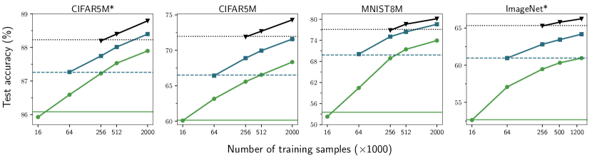
Figure 2: (Scaling number of training samples) Model centers are selected by random sub-sampling from the training data set. The baselines (lines without markers) are obtained from a standard kernel machine solved by EigenPro 2.0 over the centers and their corresponding labels. Lines with markers indicate the performance of kernel models trained with our algorithm (EigenPro 3.0) after 50 epochs.

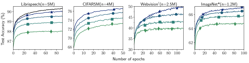
Figure 3: (Scaling model size) Performance of EigenPro 3.0 for different number of model centers, fixed number of data $n$.

Notice that this is the kernel interpolation problem EigenPro 2.0 can solve. This leads to the update,

$$\bm{\alpha}^{t+1}=\bm{\alpha}^{t}-\frac{n}{m}\eta\,\widehat{\bm{\theta}}^{T}$$ (EigenPro 3.0 update)

where $\widehat{\bm{\theta}}^{T}$ is the solution to equation 32 after $T$ steps of EigenPro 2.0 given in Algorithm 3 in the Appendix. Algorithm 2, EigenPro 3.0, implements the update above.

Remark 3 (Details on inexact-projection using EigenPro 2.0).

We apply $T$ steps of EigenPro 2.0 for the approximate projection. This algorithm itself applies a fast preconditioned SGD to solve the problem. The algorithm needs no hyperparameters adjustment. However, you need to choose $s$ and $q$. More details on this in the Appendix LABEL:choiceofhypers.

Remark 4 (Decoupling).

There are two preconditioners involved in EigenPro 3.0, a data preconditioner (for the stochastic gradient) which depends only on $X$, and a model preconditioner (for the inexact projection) which depends only on $Z$. This maintains the models decoupling from the training data.

Complexity analysis: We compare the complexity of the run-time and memory requirement of Algorithm 2 and Algorithm 1 with Falkon solver in Table 1.

6 Real data experiments

In this section, we demonstrate that our method can effectively scale both the size of the model and the number of training samples. We show that both of these factors are crucial for a better performance. We perform experiments on these datasets: (1) CIFAR10, CIFAR10 (Krizhevsky et al., 2009), (2) CIFAR5M, CIFAR5M${}^{*}$ (Nakkiran et al., 2021), (3) ImageNet${}^{*}$, (Deng et al., 2009), (4) MNIST, (LeCun, 1998), (5) MNIST8M, (Loosli et al., 2007), (6) Fashion-MNIST, (Xiao et al., 2017), (7) Webvision, (Li et al., 2017), and (8) Librispeech, (Panayotov et al., 2015). Details about datasets can be found in Appendix LABEL:sec:expt_details. Our method can be implemented with any kernel function, but for the purpose of this demonstration, we chose to use the Laplace kernel due to its simplicity and empirical effectiveness. We treat multi-class classification problems as multiple independent binary regression problems, with targets from $\left\{0,1\right\}$. The final prediction is determined by selecting the class with the highest predicted value among the $K$ classes.

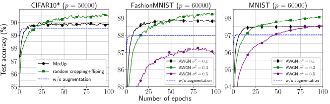
Figure 4: (Data augmentation for kernel models) Entire original dataset was used as as the model centers $Z$. The model was trained using the augmented set $X$ (without the original data). MixUp and Crop+Flip augmentation was used for CIFAR10. Additive White Gaussian Noise (AWGN) augmentation was used for MNIST and FashionMNIST.

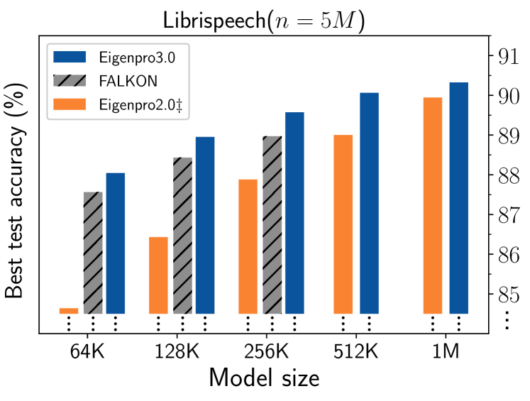
Figure 5: Comparison of EigenPro 3.0 (EP3) performance with Falkon  and EigenPro 2.0 (EP2).
${}^{\ddagger}$ For EigenPro 2.0 models size and number of training samples are the same. $n=5$M was used for all other methods. FALKON could not be run for model size larger than $256$K centers due to memory limitations. For each model size, EigenPro 2.0 and EigenPro 3.0 use the same centers.

Scaling the number of training samples: Figure 2 illustrates that for a fixed model size, increasing the number of training samples leads to a significant improvement in performance, as indicated by the the lines with marker. As a point of comparison, we also include results from a standard kernel machine using the same centers, represented by the horizontal lines without markers. In this experiment, the centers were randomly selected from the data and they are a subset of training data.

Scaling the model size: Figure 3 shows that, when the number of training samples is fixed, larger models perform significantly better.

To the best of our knowledge, Falkon  is the only method capable of training general kernel models with model size larger than $100,\!000$ centers. Our memory resources of $340$GB RAM allowed us to handle up to $256,\!000$ centers using Falkon. Figure 5 illustrates that our method outperforms Falkon  by utilizing larger models. Moreover, for a fixed set of centers, training on greater number of data will boost the performance. Therefore, EigenPro 3.0 outperforms EigenPro 2.0 by training on more data.

Data augmentation for kernel models: Data augmentation is a crucial technique for improving the performance of deep networks. We demonstrate its benefits for general kernel models by selecting the model centers $Z$ to be the original training data and the train set $X$ to be the virtual examples generated through augmentation. To the best of our knowledge, this is the first implementation of data augmentation for kernel models at this scale. Figure 4 shows we have significant improvements in accuracy.

Data processing details: We performed our experiment on CIFAR10 with feature extraction, raw images of MNIST and FashionMNIST. For CIFAR10 augmentation, we apply random cropping and flipping before feature extraction. We also apply mix-up augmentation method from (Zhang et al., 2018) after feature extraction. For MNIST and FashionMNIST augmentation we added Gaussian noise with different variances. To the best of our knowledge, this is the first implementation of data augmentation for kernel models at this scale. Figure 4 shows we have significant improvements in accuracy.

7 Conclusions and Outlook

Dataset	Model	$p=100$	$p=1000$	$p=10000$
CIFAR10	$k-$means	36.24	45.12	52.72
($n=50000$)	random	$33.37\pm 0.50$	$44.19\pm 0.09$	$49.92\pm 0.08$
CIFAR10*	$k-$means	82.69	86.58	89.11
($n=50000$)	random	$74.29\pm 0.44$	$84.38\pm 0.15$	$86.58\pm 0.06$
MNIST	$k-$means	$\boldsymbol{91.89}$	$\boldsymbol{95.96}$	$\boldsymbol{97.69}$
($n=60000$)	random	$87.24\pm 0.015$	$94.96\pm 0.102$	$97.31\pm 0.004$
FashionMNIST	$k-$means	$\boldsymbol{78.66}$	$\boldsymbol{85.55}$	$\boldsymbol{88.13}$
($n=60000$)	random	$76.24\pm 0.003$	$84.59\pm 0.069$	$87.84\pm 0.036$

Table 2: (Benefits of model flexibility) Comparison between random centers selection and k-means clustering using EigenPro 3.0. Here $p$ denotes the number of centers.
(${}^{*}$ indicates a preprocessing step.)

The remarkable success of Deep Learning has been in large part due to very large models trained on massive datasets. Any credible alternative requires a path to scaling model sizes as well as the size of the training set. Traditional kernel methods suffer from a severe scaling limitation as their model sizes are coupled to size of the training set. Yet, as we have seen in numerous experiments, performance improves with the amount of data far beyond the point where the amount of data exceeds the number of model centers. Other solvers, such as Falkon (Rudi et al., 2017), Gpytorch  (Gardner et al., 2018) GPFlow (Matthews et al., 2017), allow for unlimited data but limit the model size.

In this work we provide a proof of concept showing that for kernel methods the barrier of limited model size can be overcome. Indeed, with a fixed model size our proposed algorithm, EigenPro 3.0 has no specific limitations on the number of samples it can use in training. As a simple illustration Fig. 6 demonstrates the results of a kernel machine trained on an augmented FashionMNIST dataset with $1.2\!\times\!10^{8}$ data samples. While increasing the model size is more challenging, we have achieved 1 million centers and see no fundamental mathematical barrier to increasing the number of centers to 10 million and beyond. Furthermore, as EigenPro 3.0 is highly parallelizable, we anticipate future scaling to tens of millions of centers trained on billions of data points, approaching the scale of modern neural networks.

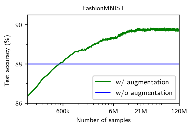
Figure 6: (Training on 120 million samples) The plot shows the results of training on 120 million data samples generated by adding Gaussian noise to the original 60,000 images. The model centers are the images.

This line of research opens a pathway for a principled alternative to deep neural networks. While in our experiments we focused primarily on Laplace kernels for their simplicity and effectiveness, recently developed kernels such as NTK, CNTK, and other neural kernels from (Shankar et al., 2020), can be used to achieve state-of-the-art performance on various datasets. Our approach is compatible with any choice of kernel, and furthermore, can be adapted to kernels that learn features, such as Recursive Feature Machines (Radhakrishnan et al., 2022a).

Finally, we note that while the set of centers $Z$ can be arbitrary, the choice of centers can affect model performance. Table 2 (see also (Que & Belkin, 2016)) demonstrates that using centers selected via the $k$-means algorithm often results in notable performance improvements when the number of centers is smaller than the number of samples. Further research should explore criteria for optimal center selection, incorporating recent advances, such as Rocket-propelled Cholesky (Chen et al., 2022), into EigenPro 3.0 to improve both model selection and construction of preconditioners.

Acknowledgments

We thank Giacomo Meanti for help with using Falkon, and Like Hui for providing us with the extracted features of the Librispeech dataset.
We are grateful for the support from the National Science Foundation (NSF) and the Simons Foundation for the Collaboration on the Theoretical Foundations of Deep Learning (https://deepfoundations.ai/) through awards DMS-2031883 and #814639 and the TILOS institute (NSF CCF-2112665). This work was done in part while the authors were visiting the Simons Institute for the Theory of Computing. This work used NVIDIA V100 GPUs NVLINK and HDR IB (Expanse GPU) at SDSC Dell Cluster through allocation TG-CIS220009 and also, Delta system at the National Center for Supercomputing Applications through allocation bbjr-delta-gpu from the Advanced Cyberinfrastructure Coordination Ecosystem: Services & Support (ACCESS) program, which is supported by National Science Foundation grants #2138259, #2138286, #2138307, #2137603, and #2138296. Prior to 09/01/2022, we used the Extreme Science and Engineering Discovery Environment (XSEDE) (Towns et al., 2014), which is supported by NSF grant number ACI-1548562, Expanse CPU/GPU compute nodes, and allocations TG-CIS210104 and TG-CIS220009.

Appendices

Table 3: Symbolic notation for EigenPro 3.0 in Algorithm 2. They satisfy $m<n$, and $q<s<n.$

Symbol	Purpose
$n$	Number of samples
$m$	Batch-size
$p$	Model size
$s$	Nyström approximation subsample size
$q$	Preconditioner level

Appendix A Fixed point analysis

Here we provide a characterization of the fixed point of Algorithm 1.

Lemma 6.

For any dataset $X,\bm{y}$ and any choice of model centers $Z$, if the learning rate satisfies

$$\eta<\frac{2}{\lambda_{\rm max}\left(K(Z,X)(I_{n}-\bm{Q})K(X,Z)\right)}$$

we have that

$$\lim_{t\rightarrow\infty}\bm{\alpha}_{t}=\left(K(Z,X)(I_{n}-\bm{Q})K(X,Z)\right)^{-1}K(Z,X)(I_{n}-\bm{Q})\bm{y}.$$

Furthermore, if $\bm{y}=K(X,Z)\bm{\alpha}^{*}+\bm{\xi}$, where $\xi_{i}$ are independent centered with $\operatorname{\mathbb{E}}|\xi_{i}|^{2}=\sigma^{2}$, then

$$\lim_{t\rightarrow\infty}\operatorname{\mathbb{E}}\alpha_{t} =\bm{\alpha}^{*}$$

$$\lim_{t\rightarrow\infty}\frac{\operatorname{\mathbb{E}}\left\|\bm{\alpha}_{t}-\bm{\alpha}^{*}\right\|^{2}}{\sigma^{2}} ={\rm tr}\left(\left(K(Z,X)(I_{n}-\bm{Q})K(X,Z)\right)^{-2}K(Z,X)(I_{n}-\bm{Q})^{2}K(X,Z)\right)$$

$$=n-{\rm trace}\left(\left(K(Z,X)(I_{n}-\bm{Q})K(X,Z)\right)^{-2}K(Z,X)\bm{Q}(I_{n}-\bm{Q})K(X,Z)\right)$$

Appendix B Proofs of intermediate results

B.1 Proof of proposition 1

Proposition (Nyström extension).

For $1\leq i\leq n$, let $\lambda_{i}$ be an eigenvalue of $\mathcal{K}$, and $\psi_{i}$ its unit ${\bm{\mathcal{H}}}$-norm eigenfunction, i.e., $\mathcal{K}\left\{\psi_{i}\right\}=\lambda_{i}\psi_{i}$. Then $\lambda_{i}$ is also an eigenvalue of $K(X,X)$. Moreover if $\bm{e}_{i},$ is its unit-norm eigenvector, i.e., $K(X,X)\bm{e}_{i}=\lambda_{i}\bm{e}_{i}$, we have,

$$\psi_{i}=K(\cdot,X)\frac{\bm{e}_{i}}{\sqrt{\lambda_{i}}}.$$ (33)

Proof.

Let $\psi\in\mathcal{H}$ be an eigenfunction of $\mathcal{K}$. Then by definition of $\mathcal{K}$ we have,

$$\lambda\psi=\mathcal{K}\left\{\psi\right\}=\sum_{i=1}^{n}K(\cdot,\bm{x}_{i})\psi(\bm{x}_{i}).$$ (34)

As the result we can write $\psi$ as below,

$$\psi=\sum_{i=1}^{n}\frac{\psi(\bm{x}_{i})}{\lambda}K(\cdot,\bm{x}_{i}).$$ (35)

If we apply covariance operator to the both side of 35 we have,

$$\mathcal{K}\left\{\psi\right\} =\mathcal{K}\left\{\sum_{i=1}^{n}\frac{\psi(\bm{x}_{i})}{\lambda}K(\cdot,\bm{x}_{i})\right\}=\sum_{i,j=1}^{n}\frac{\psi(\bm{x}_{i})}{\lambda}K(\bm{x}_{i},\bm{x}_{j})K(\cdot,\bm{x}_{j})=\sum_{j=1}^{n}\psi(\bm{x}_{j})K(\cdot,\bm{x}_{j}).$$ (36)

The last equation hold because of equation (34). If we define vector $\bm{\beta}$ such that $\bm{\beta}_{i}=\frac{\psi(x_{i})}{\lambda}$, then 36 can be rewritten as,

$$\sum_{i=1}^{n}\sum_{j=1}^{n}\bm{\beta}_{i}K(\bm{x}_{i},\bm{x}_{j})K(\cdot,\bm{x}_{i})=\lambda\sum_{i=1}^{n}\bm{\beta}_{i}K(\cdot,\bm{x}_{i}).$$ (37)

Compactly we can write 37 as below,

$$K(X,X)^{2}\bm{\beta}=\lambda K(X,X)\bm{\beta}\implies K(X,X)\bm{\beta}=\lambda\bm{\beta}.$$

The last implication holds because $K(X,X)$ is invertable. Thus $\bm{\beta}$ is an eigenvector of $K(X,X)$. It remains to determine the scale of $\bm{\beta}$.

Now, norm of $\psi$ can be simplified as

$$\left\|\psi\right\|_{\bm{\mathcal{H}}}^{2} =\left<\sum_{i=1}^{n}\beta_{i}K(\cdot,\bm{x}_{i}),\sum_{j=1}^{n}\beta_{j}K(\cdot,\bm{x}_{j})\right>_{\bm{\mathcal{H}}}$$ (38)

$$=\sum_{i,j=1}^{n}\beta_{i}\beta_{j}\left<K(\cdot,\bm{x}_{i}),K(\cdot,\bm{x}_{j})\right>_{\bm{\mathcal{H}}}=\bm{\beta}^{\top}K(X,X)\bm{\beta}=\lambda\left\|\bm{\beta}\right\|^{2}.$$ (39)

Since $\psi$ is unit norm, we have $\left\|\bm{\beta}\right\|=\frac{1}{\sqrt{\lambda}}$. This concludes the proof. $\Box$

B.2 Proof of lemma 5

Lemma (Nyström preconditioning).

Let $\bm{a}\in\mathbb{R}^{m}$, then we have that,

$$\mathcal{P}_{s}\left\{K(\cdot,X_{m})\bm{a}\right\}=K(\cdot,X_{m})\bm{a}-K(\cdot,X_{s})\bm{Q}_{s}K(X_{s},X_{m})\bm{a}.$$ (40)

Where $Q_{s}=E_{s,q}(\bm{I}_{n}-\lambda_{s,q+1}\Lambda_{s,q}^{-1})\Lambda_{s,q}^{-1}E_{s,q}^{\top}$.

Proof.

Recall that $\mathcal{P}_{s}:=\mathcal{I}-\sum_{i=1}^{q}\left(1-\frac{\lambda_{q+1}}{\lambda_{q}}\right)\psi_{i}\otimes\psi_{i}$. By this definition we can write,

$$\mathcal{P}_{s}\left(K(\cdot,X_{M})\bm{\alpha}\right) =K(\cdot,X_{M})\bm{\alpha}-\sum_{i=1}^{s}(1-\frac{\lambda_{q+1}^{s}}{\lambda_{i}^{s}})\left<\psi_{i}^{s},K(\cdot,X_{M})\bm{\alpha}\right>_{{\bm{\mathcal{H}}}}\psi_{i}^{s}$$

$$=K(\cdot,X_{M})\bm{\alpha}-\sum_{i=1}^{q}\frac{1}{\lambda_{i}^{s}}(1-\frac{\lambda_{q+1}^{s}}{\lambda_{i}^{s}})\left<{K(\cdot,X_{s})}\bm{e}_{i},K(\cdot,X_{M})\bm{\alpha}\right>_{{\bm{\mathcal{H}}}}K(\cdot,X_{s})\bm{e}_{i}$$

$$=K(\cdot,X_{M})\bm{\alpha}-\sum_{i=1}^{q}\frac{1}{\lambda_{i}^{s}}(1-\frac{\lambda_{q+1}^{s}}{\lambda_{i}})\left<{K(\cdot,X_{s})\bm{e}_{i}},K(\cdot,X_{M})\bm{\alpha}\right>_{{\bm{\mathcal{H}}}}\!K(\cdot,X_{s})\bm{e}_{i}$$

$$=K(\cdot,X_{M})\bm{\alpha}-\sum_{i=1}^{q}(1-\frac{\lambda_{q+1}^{s}}{\lambda_{i}^{s}})K(\cdot,X_{s})\bm{e}_{i}\bm{e}_{i}^{\top}K(X_{s},X_{M})\bm{\alpha}.$$

Note that we used proposition 1 for $\psi$. Now we can compactly write the last expression as below,

$$\mathcal{P}_{s}\left(K(\cdot,X_{M})\bm{\alpha}\right) =K(\cdot,X_{M})\bm{\alpha}-K(\cdot,X_{s})E_{s,q}(\bm{I}_{n}-\lambda_{s,q+1}\Lambda_{s,q}^{-1})\Lambda_{s,q}^{-1}E_{s,q}^{\top}K(X_{s},X_{M})\bm{\alpha}$$

$$=K(\cdot,X_{M})\bm{\alpha}-K(\cdot,X_{s})Q_{s}K(X_{s},X_{M})\bm{\alpha}.$$

This concludes the proof.

$\Box$

Appendix C Details on EigenPro 2.0

Algorithm 3 EigenPro 2.0$(X,\bm{y})$. Solves the linear system $K(X,X)\bm{\theta}=\bm{y}$

Data $(X,\bm{y})$, Nyström size $s$, preconditioner level $q$$\bm{\alpha}\leftarrow\textbf{0}\in\mathbb{R}^{n}$initialization $X_{s},(\bm{E},\bm{D}),\eta,m\leftarrow$EigenPro 2.0_setup($X,s,q$) Stopping criterion not reached $\bm{\alpha}\leftarrow$EigenPro 2.0_iteration$(X,\bm{y},X_{s},\bm{E},\bm{D},\bm{\alpha},m,\eta)$$\bm{\alpha}$

EigenPro2_setup$(X,s,q)$

Data $X$, Nyström size $s$, preconditioner size $q$Fetch a subsample $X_{s}\subseteq X$of size $s$

References

- Aronszajn (1950) Aronszajn, N. Theory of reproducing kernels. Transactions of the American mathematical society, 68(3):337–404, 1950.
- Arora et al. (2020) Arora, S., Du, S. S., Li, Z., Salakhutdinov, R., Wang, R., and Yu, D. Harnessing the power of infinitely wide deep nets on small-data tasks. In International Conference on Learning Representations, 2020. URL https://openreview.net/forum?id=rkl8sJBYvH.
- Baldi et al. (2014) Baldi, P., Sadowski, P., and Whiteson, D. Searching for exotic particles in high-energy physics with deep learning. Nature communications, 5(1):1–9, 2014.
- Camoriano et al. (2016) Camoriano, R., Angles, T., Rudi, A., and Rosasco, L. Nytro: When subsampling meets early stopping. In Artificial Intelligence and Statistics, pp. 1403–1411. PMLR, 2016.
- Chen et al. (2010) Chen, Y., Welling, M., and Smola, A. Super-samples from kernel herding. UAI’10: Proceedings of the Twenty-Sixth Conference on Uncertainty in Artificial Intelligence, Pages 109–116, 2010.
- Chen et al. (2022) Chen, Y., Epperly, E. N., Tropp, J. A., and Webber, R. J. Randomly pivoted cholesky: Practical approximation of a kernel matrix with few entry evaluations. arXiv preprint arXiv:2207.06503, 2022.
- Deng et al. (2009) Deng, J., Dong, W., Socher, R., Li, L.-J., Li, K., and Fei-Fei, L. Imagenet: A large-scale hierarchical image database. In 2009 IEEE conference on computer vision and pattern recognition, pp. 248–255. Ieee, 2009.
- Gardner et al. (2018) Gardner, J., Pleiss, G., Wu, R., Weinberger, K., and Wilson, A. Product kernel interpolation for scalable gaussian processes. In International Conference on Artificial Intelligence and Statistics, pp. 1407–1416. PMLR, 2018.
- Geifman et al. (2020) Geifman, A., Yadav, A., Kasten, Y., Galun, M., Jacobs, D., and Ronen, B. On the similarity between the laplace and neural tangent kernels. In Advances in Neural Information Processing Systems, 2020.
- Hoffmann et al. (2022) Hoffmann, J., Borgeaud, S., Mensch, A., Buchatskaya, E., Cai, T., Rutherford, E., de las Casas, D., Hendricks, L. A., Welbl, J., Clark, A., Hennigan, T., Noland, E., Millican, K., van den Driessche, G., Damoc, B., Guy, A., Osindero, S., Simonyan, K., Elsen, E., Vinyals, O., Rae, J. W., and Sifre, L. An empirical analysis of compute-optimal large language model training. In Oh, A. H., Agarwal, A., Belgrave, D., and Cho, K. (eds.), Advances in Neural Information Processing Systems, 2022. URL https://openreview.net/forum?id=iBBcRUlOAPR.
- Hui & Belkin (2021) Hui, L. and Belkin, M. Evaluation of neural architectures trained with square loss vs cross-entropy in classification tasks. In International Conference on Learning Representations, 2021. URL https://openreview.net/forum?id=hsFN92eQEla.
- Jacot et al. (2018) Jacot, A., Gabriel, F., and Hongler, C. Neural tangent kernel: Convergence and generalization in neural networks. Advances in neural information processing systems, 31, 2018.
- Jurafsky (2000) Jurafsky, D. Speech & language processing. Pearson Education India, 2000.
- Kaplan et al. (2020) Kaplan, J., McCandlish, S., Henighan, T., Brown, T. B., Chess, B., Child, R., Gray, S., Radford, A., Wu, J., and Amodei, D. Scaling laws for neural language models. arXiv preprint arXiv:2001.08361, 2020.
- Kimeldorf & Wahba (1970) Kimeldorf, G. S. and Wahba, G. A correspondence between bayesian estimation on stochastic processes and smoothing by splines. The Annals of Mathematical Statistics, 41(2):495–502, 1970.
- Krizhevsky et al. (2009) Krizhevsky, A., Hinton, G., et al. Learning multiple layers of features from tiny images. Citeseer, 2009.
- Krizhevsky et al. (2012) Krizhevsky, A., Sutskever, I., and Hinton, G. E. Imagenet classification with deep convolutional neural networks. In Pereira, F., Burges, C., Bottou, L., and Weinberger, K. (eds.), Advances in Neural Information Processing Systems, volume 25. Curran Associates, Inc., 2012. URL https://proceedings.neurips.cc/paper/2012/file/c399862d3b9d6b76c8436e924a68c45b-Paper.pdf.
- LeCun (1998) LeCun, Y. The mnist database of handwritten digits. http://yann. lecun. com/exdb/mnist/, 1998.
- Lee et al. (2020) Lee, J., Schoenholz, S., Pennington, J., Adlam, B., Xiao, L., Novak, R., and Sohl-Dickstein, J. Finite versus infinite neural networks: an empirical study. Advances in Neural Information Processing Systems, 33:15156–15172, 2020.
- Li et al. (2017) Li, W., Wang, L., Li, W., Agustsson, E., and Van Gool, L. Webvision database: Visual learning and understanding from web data. arXiv preprint arXiv:1708.02862, 2017.
- Li et al. (2019) Li, Z., Wang, R., Yu, D., Du, S. S., Hu, W., Salakhutdinov, R., and Arora, S. Enhanced convolutional neural tangent kernels. arXiv preprint arXiv:1911.00809, 2019.
- Loosli et al. (2007) Loosli, G., Canu, S., and Bottou, L. Training invariant support vector machines using selective sampling. Large scale kernel machines, 2, 2007.
- Ma & Belkin (2017) Ma, S. and Belkin, M. Diving into the shallows: a computational perspective on large-scale shallow learning. Advances in neural information processing systems, 30, 2017.
- Ma & Belkin (2019) Ma, S. and Belkin, M. Kernel machines that adapt to gpus for effective large batch training. Proceedings of Machine Learning and Systems, 1:360–373, 2019.
- Ma et al. (2018) Ma, S., Bassily, R., and Belkin, M. The power of interpolation: Understanding the effectiveness of sgd in modern over-parametrized learning. International Conference on Machine Learning, pp. 3325–3334, 2018.
- Matthews et al. (2017) Matthews, A. G. d. G., van der Wilk, M., Nickson, T., Fujii, K., Boukouvalas, A., León-Villagrá, P., Ghahramani, Z., and Hensman, J. GPflow: A Gaussian process library using TensorFlow. Journal of Machine Learning Research, 18(40):1–6, apr 2017. URL http://jmlr.org/papers/v18/16-537.html.
- Meanti et al. (2020) Meanti, G., Carratino, L., Rosasco, L., and Rudi, A. Kernel methods through the roof: handling billions of points efficiently. Advances in Neural Information Processing Systems, 33:14410–14422, 2020.
- Nakkiran et al. (2021) Nakkiran, P., Neyshabur, B., and Sedghi, H. The deep bootstrap framework: Good online learners are good offline generalizers. International Conference on Learning Representations, 2021.
- Panayotov et al. (2015) Panayotov, V., Chen, G., Povey, D., and Khudanpur, S. Librispeech: an asr corpus based on public domain audio books. In 2015 IEEE international conference on acoustics, speech and signal processing (ICASSP), pp. 5206–5210. IEEE, 2015.
- Pedregosa et al. (2011) Pedregosa, F., Varoquaux, G., Gramfort, A., Michel, V., Thirion, B., Grisel, O., Blondel, M., Prettenhofer, P., Weiss, R., Dubourg, V., Vanderplas, J., Passos, A., Cournapeau, D., Brucher, M., Perrot, M., and Duchesnay, E. Scikit-learn: Machine learning in Python. Journal of Machine Learning Research, 12:2825–2830, 2011.
- Poggio & Girosi (1990) Poggio, T. and Girosi, F. Networks for approximation and learning. Proceedings of the IEEE, 78(9):1481–1497, 1990.
- Que & Belkin (2016) Que, Q. and Belkin, M. Back to the future: Radial basis function networks revisited. In Artificial intelligence and statistics, pp. 1375–1383. PMLR, 2016.
- Radhakrishnan et al. (2022a) Radhakrishnan, A., Beaglehole, D., Pandit, P., and Belkin, M. Feature learning in neural networks and kernel machines that recursively learn features. arXiv preprint arXiv:2212.13881, 2022a.
- Radhakrishnan et al. (2022b) Radhakrishnan, A., Stefanakis, G., Belkin, M., and Uhler, C. Simple, fast, and flexible framework for matrix completion with infinite width neural networks. Proceedings of the National Academy of Sciences, 119(16):e2115064119, 2022b.
- Rahimi & Recht (2007) Rahimi, A. and Recht, B. Random features for large-scale kernel machines. Advances in neural information processing systems, 20, 2007.
- Richardson (1911) Richardson, L. F. Ix. the approximate arithmetical solution by finite differences of physical problems involving differential equations, with an application to the stresses in a masonry dam. Philosophical Transactions of the Royal Society of London. Series A, Containing Papers of a Mathematical or Physical Character, 210(459-470):307–357, 1911.
- Rudi et al. (2017) Rudi, A., Carratino, L., and Rosasco, L. Falkon: An optimal large scale kernel method. Advances in neural information processing systems, 30, 2017.
- Schölkopf et al. (2002) Schölkopf, B., Smola, A. J., Bach, F., et al. Learning with kernels: support vector machines, regularization, optimization, and beyond. MIT press, 2002.
- Shalev-Shwartz et al. (2007) Shalev-Shwartz, S., Singer, Y., and Srebro, N. Pegasos: Primal estimated sub-gradient solver for svm. In Proceedings of the 24th international conference on Machine learning, pp. 807–814, 2007.
- Shankar et al. (2020) Shankar, V., Fang, A., Guo, W., Fridovich-Keil, S., Ragan-Kelley, J., Schmidt, L., and Recht, B. Neural kernels without tangents. In International Conference on Machine Learning, pp. 8614–8623. PMLR, 2020.
- Titsias (2009) Titsias, M. Variational learning of inducing variables in sparse gaussian processes. In Artificial intelligence and statistics, pp. 567–574. PMLR, 2009.
- Towns et al. (2014) Towns, J., Cockerill, T., Dahan, M., Foster, I., Gaither, K., Grimshaw, A., Hazlewood, V., Lathrop, S., Lifka, D., Peterson, G. D., Roskies, R., Scott, J., and Wilkins-Diehr, N. Xsede: Accelerating scientific discovery. Computing in Science & Engineering, 16(05):62–74, sep 2014. ISSN 1558-366X. doi: 10.1109/MCSE.2014.80.
- Virtanen et al. (2020) Virtanen, P., Gommers, R., Oliphant, T. E., Haberland, M., Reddy, T., Cournapeau, D., Burovski, E., Peterson, P., Weckesser, W., Bright, J., van der Walt, S. J., Brett, M., Wilson, J., Millman, K. J., Mayorov, N., Nelson, A. R. J., Jones, E., Kern, R., Larson, E., Carey, C. J., Polat, İ., Feng, Y., Moore, E. W., VanderPlas, J., Laxalde, D., Perktold, J., Cimrman, R., Henriksen, I., Quintero, E. A., Harris, C. R., Archibald, A. M., Ribeiro, A. H., Pedregosa, F., van Mulbregt, P., and SciPy 1.0 Contributors. SciPy 1.0: Fundamental Algorithms for Scientific Computing in Python. Nature Methods, 17:261–272, 2020. doi: 10.1038/s41592-019-0686-2.
- Watanabe et al. (2018) Watanabe, S., Hori, T., Karita, S., Hayashi, T., Nishitoba, J., Unno, Y., Enrique Yalta Soplin, N., Heymann, J., Wiesner, M., Chen, N., Renduchintala, A., and Ochiai, T. ESPnet: End-to-end speech processing toolkit. In Proceedings of Interspeech, pp. 2207–2211, 2018. doi: 10.21437/Interspeech.2018-1456. URL http://dx.doi.org/10.21437/Interspeech.2018-1456.
- Wightman (2019) Wightman, R. Pytorch image models. https://github.com/rwightman/pytorch-image-models, 2019.
- Williams & Seeger (2000) Williams, C. and Seeger, M. Using the nyström method to speed up kernel machines. Advances in neural information processing systems, 13, 2000.
- Wilson & Nickisch (2015) Wilson, A. and Nickisch, H. Kernel interpolation for scalable structured gaussian processes (kiss-gp). In International conference on machine learning, pp. 1775–1784. PMLR, 2015.
- Xiao et al. (2017) Xiao, H., Rasul, K., and Vollgraf, R. Fashion-mnist: a novel image dataset for benchmarking machine learning algorithms. arXiv preprint arXiv:1708.07747, 2017.
- Yang et al. (2012) Yang, T., Li, Y.-F., Mahdavi, M., Jin, R., and Zhou, Z.-H. Nyström method vs random fourier features: A theoretical and empirical comparison. Advances in neural information processing systems, 25, 2012.
- Zhang et al. (2018) Zhang, H., Cisse, M., Dauphin, Y. N., and Lopez-Paz, D. mixup: Beyond empirical risk minimization. International Conference on Learning Representations, 2018.
- Zhu et al. (2022) Zhu, L., Liu, C., and Belkin, M. Transition to linearity of general neural networks with directed acyclic graph architecture. Advances in neural information processing systems, 2022.