Learning Representations of Bi-level Knowledge Graphs for
Reasoning beyond Link Prediction

Abstract

Knowledge graphs represent known facts using triplets. While existing knowledge graph embedding methods only consider the connections between entities, we propose considering the relationships between triplets. For example, let us consider two triplets $T_{1}$ and $T_{2}$ where $T_{1}$ is (Academy_Awards, Nominates, Avatar) and $T_{2}$ is (Avatar, Wins, Academy_Awards). Given these two base-level triplets, we see that $T_{1}$ is a prerequisite for $T_{2}$. In this paper, we define a higher-level triplet to represent a relationship between triplets, e.g., $\langle T_{1}$, PrerequisiteFor, $T_{2}\rangle$ where PrerequisiteFor is a higher-level relation. We define a bi-level knowledge graph that consists of the base-level and the higher-level triplets. We also propose a data augmentation strategy based on the random walks on the bi-level knowledge graph to augment plausible triplets. Our model called BiVE learns embeddings by taking into account the structures of the base-level and the higher-level triplets, with additional consideration of the augmented triplets. We propose two new tasks: triplet prediction and conditional link prediction. Given a triplet $T_{1}$ and a higher-level relation, the triplet prediction predicts a triplet that is likely to be connected to $T_{1}$ by the higher-level relation, e.g., $\langle T_{1}$, PrerequisiteFor, ?$\rangle$. The conditional link prediction predicts a missing entity in a triplet conditioned on another triplet, e.g., $\langle T_{1}$, PrerequisiteFor, (Avatar, Wins, ?)$\rangle$. Experimental results show that BiVE significantly outperforms all other methods in the two new tasks and the typical base-level link prediction in real-world bi-level knowledge graphs.

Introduction

A knowledge graph represents the relationships between entities using triplets consisting of a head entity, a relation, and a tail entity. Knowledge graph embedding aims to represent the entities and relations as a set of embedding vectors that can be utilized in many modern AI applications [17, 20]. Most existing knowledge graph embedding methods generate the embedding vectors by focusing solely on how the entities are connected by the relations [36, 6, 4]. Even though some methods predict missing connections between the entities by rule mining [27, 31] or rule-and-path-based learning [29], these existing approaches only enable expanding the entity-level connections.

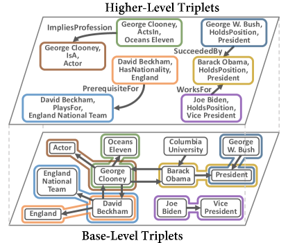
Figure 1: Example of a bi-level knowledge graph consisting of base-level and higher-level triplets in the FBHE dataset. The relation labels are omitted in the base-level triplets.

Each triplet in a knowledge graph can have a relationship with another triplet. For example, let us consider two base-level triplets $T_{1}$ and $T_{2}$ where $T_{1}$ is (Joe_Biden, HoldsPosition, Vice_President) and $T_{2}$ is (Barack_Obama, HoldsPosition, President). To represent the fact that Joe Biden was a vice president when Barack Obama was a president, we define a higher-level triplet $\langle T_{1}$, WorksFor, $T_{2}\rangle$ where WorksFor is a higher-level relation. In this paper, we define a bi-level knowledge graph that includes both the base-level and the higher-level triplets, where the base-level triplets correspond to the original triplets representing the relationships between entities, while the higher-level triplets represent the relationships between the base-level triplets using the higher-level relations. Based on well-known knowledge graphs, FB15K237 [34] and DB15K [11], we create three real-world bi-level knowledge graphs named FBH, FBHE, and DBHE. Figure 1 shows a subgraph of a bi-level knowledge graph in FBHE where the base-level triplets correspond to the original triplets in FB15K237 and the higher-level triplets are manually created by defining the higher-level relationships between the base-level triplets.

We propose incorporating the base-level and the higher-level triplets into knowledge graph embedding. Using the bi-level knowledge graphs, we also propose a data augmentation strategy that augments triplets by identifying plausible relation sequences based on random walks. We develop a new knowledge graph embedding method called BiVE (embedding of Bi-leVel knowledgE graphs) that computes embedding vectors by reflecting the structures of the base-level and the higher-level triplets simultaneously, where the augmented triplets are further incorporated. Using the bi-level knowledge graphs, we propose two new tasks: triplet prediction and conditional link prediction. The triplet prediction predicts a triplet that is likely to be connected to a given triplet using a higher-level relation, e.g., $\langle T_{1}$, WorksFor, ?$\rangle$, whereas the conditional link prediction predicts a missing entity in a triplet where another triplet is provided as a condition, e.g., $\langle T_{1}$, WorksFor, (?, HoldsPosition, President)$\rangle$. Experimental results show that BiVE significantly outperforms other state-of-the-art knowledge graph completion methods in real-world datasets.

Our contributions can be summarized as follows:

• To the best of our knowledge, our work is the first work that introduces the higher-level relationships between triplets in knowledge graphs; we define bi-level knowledge graphs and create three real-world datasets.

• We propose an efficient data augmentation strategy using random walks on a bi-level knowledge graph.

• We develop BiVE to learn embeddings by effectively incorporating the base-level triplets, the higher-level triplets, and the augmented triplets.

• We propose two new tasks, triplet prediction and conditional link prediction, which have never been studied.

• BiVE significantly outperforms 12 different state-of-the-art knowledge graph completion methods.

Related Work

Some knowledge graph completion methods use multi-hop paths between distant entities [29, 25, 18, 24, 7] and rule-based or logic-based methods identify frequently observed patterns [27, 8, 13, 39, 31, 28]. The main difference between these methods and BiVE is that the existing methods only consider the relationships between entities, whereas BiVE considers not only the relationships between entities but also the relationships between triplets. Also, the way of expressing the relationships between entities or triplets in BiVE is not restricted to the first-order-logic-like expression. For example, the rule-based methods consider the relationships between connected entities, e.g., $\forall x,y,z:(x,r_{1},y)\wedge(y,r_{2},z)\Rightarrow(x,r_{3},z)$ where there should exist a path connecting $x$, $y$, and $z$ in the knowledge graph. On the other hand, BiVE represents relationships like $(x,r_{1},y)\xRightarrow{\widehat{r}}(p,r_{2},q)$ where $x$, $y$ and $p$, $q$ are not necessarily connected by the base-level triplets, and also $r_{1}$, $r_{2}$, and $\xRightarrow{\widehat{r}}$ can be any relation not restricted to the first-order-logic-like relation.

Even though there have been many attempts to discover meaningful patterns in a knowledge graph and utilize them to complete missing links [21], such attempts have rarely been studied in the context of data augmentation. Recently, rule-based data augmentation for knowledge graph embedding has been proposed [23]. While this method uses logical rules using the base-level triplets, our data augmentation employs random walks on a bi-level knowledge graph.

To exploit enriched information about triplets, some knowledge graph embedding methods utilize attributes of entities or ontological concepts [15]. TransEA [37] considers numeric attributes of entities, and LiteralE [19] considers information from literals. HINGE [30] has been proposed to represent hyper-relational facts where a triplet has additional key-value pairs to present extra information about each triplet. Even though these methods consider enriched information about triplets, they do not consider the relationships between triplets.

In information retrieval, a neural fact contextualization method has been proposed to rank a set of candidate facts for a given triplet [35]. Also, a way of representing a triplet in an embedding space is studied by considering the concept of a line graph [10]. Recently, ATOMIC [32] has been proposed to provide commonsense knowledge for if-then reasoning, whereas ASER [41] has been proposed to construct an eventuality knowledge graph. Although these methods consider triplet-level operations, the goal of their methods is different from ours and none of these considers the bi-level knowledge graphs.

Bi-Level Knowledge Graphs

Let us represent a knowledge graph as $G=(\mathcal{V},\mathcal{R},\mathcal{E})$ where $\mathcal{V}$ is a set of entities, $\mathcal{R}$ is a set of relations, and $\mathcal{E}=\{(h,r,t):h\in\mathcal{V},r\in\mathcal{R},t\in\mathcal{V}\}$ is a set of triplets. Let us call $G$ a base-level knowledge graph and call $(h,r,t)\in\mathcal{E}$ a base-level triplet. We formally define the higher-level triplets as follows.

Definition 1 (Higher-Level Triplets)

Given a base-level knowledge graph $G=(\mathcal{V},\mathcal{R},\mathcal{E})$, a set of higher-level triplets is defined by $\mathcal{H}=\{\langle T_{i},\widehat{r},T_{j}\rangle:T_{i}\in\mathcal{E},\widehat{r}\in\widehat{\mathcal{R}},T_{j}\in\mathcal{E}\}$ where $\mathcal{E}$ is a set of base-level triplets and $\widehat{\mathcal{R}}$ is a set of higher-level relations connecting the base-level triplets.

We define a bi-level knowledge graph as follows.

Definition 2 (Bi-Level Knowledge Graph)

Given a base-level knowledge graph $G=(\mathcal{V},\mathcal{R},\mathcal{E})$, a set of higher-level relations $\widehat{\mathcal{R}}$, and a set of higher-level triplets $\mathcal{H}$, a bi-level knowledge graph is defined as $\widehat{G}=(\mathcal{V},\mathcal{R},\mathcal{E},\widehat{\mathcal{R}},\mathcal{H})$.

To define a bi-level knowledge graph, we add the higher-level triplets $\mathcal{H}$ to the base-level knowledge graph $G$ by introducing the higher-level relations $\widehat{\mathcal{R}}$. We create real-world bi-level knowledge graphs FBH and FBHE based on FB15K237 from Freebase [2] and DBHE based on DB15K from DBpedia [1]. Table 1 shows some examples of the higher-level relations and triplets. FBH contains the higher-level relations that can be inferred inside the base-level knowledge graph, e.g., PrerequisiteFor and ImpliesProfession, whereas FBHE and DBHE contain some externally-sourced knowledge, e.g., WorksFor and NextAlmaMater. For example, we crawl Wikipedia articles to find information about the (vice)presidents of the United States and the alma mater information of politicians. As a result, FBH contains six different higher-level relations, FBHE has ten higher-level relations, and DBHE has eight higher-level relations. Note that the base-level knowledge graphs of FBH and FBHE are FB15K237. FBHE extends FBH by including the externally-sourced higher-level relationships. The authors of this paper manually defined the higher-level relations and added the higher-level triplets to FB15K237 and DB15K, which took six weeks.

	$\widehat{r}$	$\langle T_{i},\widehat{r},T_{j}\rangle$
FBHE	PrerequisiteFor	$T_{i}$: (BAFTA_Award, Nominates, The_King’s_Speech)
		$T_{j}$: (The_King’s_Speech, Wins, BAFTA_Award)
2-3	ImpliesProfession	$T_{i}$: (Liam_Neeson, ActsIn, Love_Actually)
		$T_{j}$: (Liam_Neeson, IsA, Actor)
2-3	WorksFor	$T_{i}$: (Joe_Biden, HoldsPosition, Vice_President)
		$T_{j}$: (Barack_Obama, HoldsPosition, President)
2-3	SucceededBy	$T_{i}$: (George_W._Bush, HoldsPosition, President)
		$T_{j}$: (Barack_Obama, HoldsPosition, President)
1-3 DBHE	ImpliesTimeZone	$T_{i}$: (Czech_Republic, TimeZone, Central_European)
		$T_{j}$: (Prague, TimeZone, Central_European)
2-3	NextAlmaMater	$T_{i}$: (Gerald_Ford, StudiesIn, University_of_Michigan)
		$T_{j}$: (Gerald_Ford, StudiesIn, Yale_University)

Table 1: Examples of Higher-Level Relations and Triplets.

Using a bi-level knowledge graph, we define the triplet prediction problem as follows.

Definition 3 (Triplet Prediction)

Given a bi-level knowledge graph $\widehat{G}=(\mathcal{V},\mathcal{R},\mathcal{E},\widehat{\mathcal{R}},\mathcal{H})$ where $\mathcal{H}=\{\langle T_{i},\widehat{r},T_{j}\rangle:T_{i}\in\mathcal{E},\widehat{r}\in\widehat{\mathcal{R}},T_{j}\in\mathcal{E}\}$, the triplet prediction problem is defined as $\langle T_{i},\widehat{r},?\rangle$ or $\langle?,\widehat{r},T_{j}\rangle$ where the goal is to predict the missing base-level triplet.

Also, we define the conditional link prediction as follows.

Definition 4 (Conditional Link Prediction)

Given a bi-level knowledge graph $\widehat{G}=(\mathcal{V},\mathcal{R},\mathcal{E},\widehat{\mathcal{R}},\mathcal{H})$ where $\mathcal{H}=\{\langle T_{i},\widehat{r},T_{j}\rangle:T_{i}\in\mathcal{E},\widehat{r}\in\widehat{\mathcal{R}},T_{j}\in\mathcal{E}\}$, let $T_{i}\coloneqq(h_{i},r_{i},t_{i})$ and $T_{j}\coloneqq(h_{j},r_{j},t_{j})$. The conditional link prediction problem is to predict a missing entity in a base-level triplet conditioned on another base-level triplet. Specifically, the problem is defined as $\langle T_{i},\widehat{r},(h_{j},r_{j},?)\rangle$ or $\langle T_{i},\widehat{r},(?,r_{j},t_{j})\rangle$ or $\langle(h_{i},r_{i},?),\widehat{r},T_{j}\rangle$ or $\langle(?,r_{i},t_{i}),\widehat{r},T_{j}\rangle$.

Data Augmentation by Random Walks on a Bi-Level Knowledge Graph

Consider a bi-level knowledge graph in the training set $\widehat{G}_{\text{train}}=(\mathcal{V},\mathcal{R},\mathcal{E}_{\text{train}},\widehat{\mathcal{R}},\mathcal{H}_{\text{train}})$ where $\mathcal{E}_{\text{train}}$ and $\mathcal{H}_{\text{train}}$ are the base-level and the higher-level triplets in the training set respectively. We add reverse relations to $\mathcal{R}$ and add reversed triplets to $\mathcal{E}_{\text{train}}$, i.e., for every $r\in\mathcal{R}$, we add $r^{-1}$ that has the reverse direction of $r$ and for every $(h,r,t)\in\mathcal{E}_{\text{train}}$, we add $(t,r^{-1},h)$ to $\mathcal{E}_{\text{train}}$. Similarly, for every $\widehat{r}\in\widehat{\mathcal{R}}$, we add $\widehat{r}^{-1}$ and add the reversed higher-level triplets to $\mathcal{H}_{\text{train}}$. All these reverse relations and reversed triplets are added only for data augmentation.

From an entity $h$, we randomly visit one of its neighbors by following a base-level or a higher-level triplet. To search for diverse patterns, we do not allow going back to an entity that has already been visited. Let us define a random walk path to be the sequence of visited entities, visited relations, and visited higher-level relations. Consider two base-level triplets $T_{i}=(h_{i},r_{i},t_{i})$ and $T_{j}=(h_{j},r_{j},t_{j})$ and a higher-level triplet $\langle T_{i},\widehat{r},T_{j}\rangle$. From any entity in $T_{i}$, we can go to any entity in $T_{j}$ and vice versa by following $r_{i}$, $\widehat{r}$, and $r_{j}$ or their reverse relations. For example, one possible random walk path is $(h_{i},r_{i},\widehat{r},r_{j},t_{j})$. Another possible random walk path is $(t_{j},r_{j}^{-1},\widehat{r}^{-1},r_{i},t_{i})$. Assume that we have a base-level triplet $T_{0}=(h_{0},r_{0},h_{i})$. Starting from $h_{0}$, we can make a longer path, e.g., $(h_{0},r_{0},h_{i},r_{i},\widehat{r},r_{j},t_{j})$. We define the length of a random walk path to be the number of entities in the sequence except the starting entity.

Given the maximum length of a random walk path $L$, we repeat the random walks by varying the length $l=2,\cdots{},L$ and repeat the random walks $n$ times for every $l$. In our experiments, we set $L$=3 and $n$=50,000,000. Let $w$ denote the sequence of a random walk path of all possible lengths, where we randomly select a starting entity for every $w$. If there are multiple identical random walk paths, we remove the duplicates to prevent unexpected bias. Let $p_{k}$ be the $k$-th unique sequence of relations and higher-level relations extracted from $w$, i.e., we make $p_{k}$ by removing all entities from $w$, e.g., if $w=(h_{0},r_{0},h_{i},r_{i},\widehat{r},r_{j},t_{j})$ then $p_{k}=(r_{0},r_{i},\widehat{r},r_{j})$. We call $p_{k}$ the relation sequence. Since $p_{k}$ only traces the relations, different random walk paths can be mapped into the same $p_{k}$. Using $p_{k}$, we rewrite a random walk path $w=(h,\cdots{},t)$ to $w=(h,p_{k},t)$ where the relation sequence of the original path $w$ is mapped into $p_{k}$, $h$ is the starting entity and $t$ is the last entity. Let $\mathcal{W}$ denote the multiset of all random walk paths of all possible lengths. We define the confidence score of $(p_{k},r)$ as

$$c(p_{k},r)\coloneqq\dfrac{|\{(h,r,t):(h,p_{k},t)\in\mathcal{W},(h,r,t)\in\mathcal{E}_{\text{train}}\}|}{|\{(h,p_{k},t):(h,p_{k},t)\in\mathcal{W}\}|}.$$

We select the pairs of $(p_{k},r)$ that satisfies $c(p_{k},r)\geq\tau$ where we set $\tau=0.7$. Let $\mathcal{S}_{kr}\coloneqq\{(h,r,t):(h,p_{k},t)\in\mathcal{W},c(p_{k},r)\geq\tau,(h,r,t)\notin\mathcal{E}_{\text{train}}\}$ where $\mathcal{S}_{kr}$ indicates a set of missing triplets $(h,r,t)$ even though $c(p_{k},r)\geq\tau$. Then, let $\mathcal{S}\coloneqq\cup_{k}\cup_{r}\mathcal{S}_{kr}$ where $\mathcal{S}$ is a set of augmented triplets. We add the triplets in $\mathcal{S}$ to a bi-level knowledge graph to augment triplets that are likely to be present. Figure 2 shows an example of a random walk path of length $2$ and an augmented triplet in FBH, where the walk starts from Bryan_Ferry. Let $p_{1}=$ (ActsIn, ActsIn^-1, ImpliesProfession, IsA). Since the confidence score of ($p_{1}$, IsA) is $0.99$, we add a triplet (Bryan_Ferry, IsA, Actor) which was missing in the original training set.

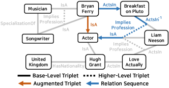
Figure 2: Random walk path in a bi-level knowledge graph and an augmented triplet in FBH. We add missing triplets whose confidence scores are greater than a certain threshold.

Embedding of Bi-Level Knowledge Graphs

A knowledge graph embedding method defines a scoring function $f({\bf{h}},{\bf{r}},{\bf{t}})$ of a triplet $(h,r,t)$, where ${\bf{h}}$, ${\bf{r}}$, and ${\bf{t}}$ are embedding vectors of $h$, $r$, and $t$ respectively; a higher score indicates a more plausible triplet. In BiVE, the loss incurred by the base-level triplets, $L_{\text{base}}$, is defined as follows:

$$L_{\text{base}}\coloneqq\sum_{(h,r,t)\in\mathcal{E}_{\text{train}}}g(-f({\bf{h}},{\bf{r}},{\bf{t}}))+\sum_{(h^{\prime},r^{\prime},t^{\prime})\in\mathcal{E}_{\text{\text{train}}}^{\prime}}g(f({\bf{h}}^{\prime},{\bf{r}}^{\prime},{\bf{t}}^{\prime}))$$

where $g(x)=\text{log}(1+\text{exp}(x))$ and $\mathcal{E}_{\text{\text{train}}}^{\prime}$ is a set of corrupted triplets. We can use any knowledge graph embedding scoring function for $f(\cdot)$. We implement BiVE with two different scoring functions for $f(\cdot)$: QuatE [42] for BiVE-Q and BiQUE [12] for BiVE-B.

Given $T_{i}=(h_{i},r_{i},t_{i})$, let ${\bf{T}}_{i}$ denote an embedding vector of $T_{i}$ where the dimension is $\hat{d}$. We define ${\bf{T}}_{i}\coloneqq\boldsymbol{W}[{\bf{h}}_{i};{\bf{r}}_{i};{\bf{t}}_{i}]$ where ${\bf{h}}_{i}$, ${\bf{r}}_{i}$, and ${\bf{t}}_{i}$ denote the embedding vectors of $h_{i}$, $r_{i}$, and $t_{i}$ respectively, the dimension of each of these embedding vectors is $d$, and $\boldsymbol{W}$ is a projection matrix of size $\hat{d}\times 3d$ which projects the vertically concatenated vector to the $\hat{d}$-dimensional space. Similarly, ${\bf{T}}_{j}=\boldsymbol{W}[{\bf{h}}_{j};{\bf{r}}_{j};{\bf{t}}_{j}]$ where $T_{j}=(h_{j},r_{j},t_{j})$. We define the loss incurred by the higher-level triplets, $L_{\text{high}}$, as follows:

$$L_{\text{high}}\coloneqq\sum_{\langle T_{i},\widehat{r},T_{j}\rangle}g(-f({\bf{T}}_{i},{\bf{\widehat{r}}},{\bf{T}}_{j}))+\sum_{\langle{T_{i}}^{\prime},\widehat{r}^{\prime},{T_{j}}^{\prime}\rangle}g(f({\bf{T}}_{i}^{\prime},{\bf{\widehat{r}}}^{\prime},{\bf{T}}_{j}^{\prime}))$$

where $\langle T_{i},\widehat{r},T_{j}\rangle\in\mathcal{H}_{\text{train}}$, $\langle{T_{i}}^{\prime},\widehat{r}^{\prime},{T_{j}}^{\prime}\rangle\in\mathcal{H}_{\text{train}}^{\prime}$, ${\bf{\widehat{r}}}$ is the embedding vector of $\widehat{r}$, the dimension of ${\bf{\widehat{r}}}$ is $\hat{d}$, and $\langle{T_{i}}^{\prime},\widehat{r}^{\prime},{T_{j}}^{\prime}\rangle$ is a corrupted higher-level triplet made by randomly replacing $T_{i}$ or $T_{j}$ with one of the triplets in $\mathcal{E}_{\text{train}}$.

We define the loss of the augmented triplets, $L_{\text{aug}}$, as

$$L_{\text{aug}}\coloneqq\sum_{(h,r,t)\in\mathcal{S}}g(-f({\bf{h}},{\bf{r}},{\bf{t}}))+\sum_{(h^{\prime},r^{\prime},t^{\prime})\in\mathcal{S}^{\prime}}g(f({\bf{h}}^{\prime},{\bf{r}}^{\prime},{\bf{t}}^{\prime}))$$

where $\mathcal{S}$ is the set of the augmented triplets and $\mathcal{S}^{\prime}$ is the set of corrupted triplets.

Finally, our loss function of BiVE is defined by

$$L_{\text{{BiVE}}}\coloneqq L_{\text{base}}+\lambda_{1}\cdot L_{\text{high}}+\lambda_{2}\cdot L_{\text{aug}}$$

where $\lambda_{1}$ is a hyperparameter indicating the importance of the higher-level triplets and $\lambda_{2}$ indicates the importance of the augmented triplets. By optimizing $L_{\text{{BiVE}}}$, BiVE learns embeddings by considering the structures of the base-level triplets, the higher-level triplets, and the augmented triplets.

Let us describe the scoring functions of BiVE for triplet prediction and conditional link prediction. To solve a triplet prediction problem, $\langle T_{i},\widehat{r},?\rangle$, we compute $F_{\text{tp}}(X)\coloneqq f({\bf{T}}_{i},{\bf{\widehat{r}}},{\bf{X}})$ for every base-level triplet $X\in\mathcal{E}_{\text{train}}$ where ${\bf{X}}$ is a learned embedding vector of $X$. To solve a conditional link prediction problem, $\langle T_{i},\widehat{r},(h_{j},r_{j},?)\rangle$, we compute $F_{\text{clp}}(x)\coloneqq f({\bf{h}}_{j},{\bf{r}}_{j},{\bf{x}})+\lambda_{1}\cdot f({\bf{T}}_{i},{\bf{\widehat{r}}},\boldsymbol{W}[{\bf{h}}_{j};{\bf{r}}_{j};{\bf{x}}])$ for every $x\in\mathcal{V}$ where ${\bf{x}}$ is a learned embedding of $x$.

	$|\mathcal{V}|$	$|\mathcal{R}|$	$|\mathcal{E}|$	$|\widehat{\mathcal{R}}|$	$|\mathcal{H}|$	$|\widehat{\mathcal{E}}|$
FBH	14,541	237	310,116	6	27,062	33,157
FBHE	14,541	237	310,116	10	34,941	33,719
DBHE	12,440	87	68,296	8	6,717	8,206

Table 2: Statistics of a bi-level knowledge graph $\widehat{G}=(\mathcal{V},\mathcal{R},\mathcal{E},\widehat{\mathcal{R}},\mathcal{H})$. $|\widehat{\mathcal{E}}|$ is the number of base-level triplets which are involved in the higher-level triplets.

	FBH			FBHE			DBHE
	MR ($\downarrow$)	MRR ($\uparrow$)	Hit@10 ($\uparrow$)	MR ($\downarrow$)	MRR ($\uparrow$)	Hit@10 ($\uparrow$)	MR ($\downarrow$)	MRR ($\uparrow$)	Hit@10 ($\uparrow$)
ASER	74541.7$\pm$0.0	0.011$\pm$0.000	0.015$\pm$0.000	57916.0$\pm$0.0	0.050$\pm$0.000	0.070$\pm$0.000	18157.6$\pm$0.0	0.042$\pm$0.000	0.075$\pm$0.000
MINERVA	109055.1$\pm$98.5	0.093$\pm$0.002	0.113$\pm$0.002	85571.5$\pm$768.3	0.220$\pm$0.008	0.300$\pm$0.005	20764.3$\pm$72.3	0.177$\pm$0.005	0.221$\pm$0.004
Multi-Hop	108731.7$\pm$43.2	0.105$\pm$0.001	0.117$\pm$0.000	83643.8$\pm$33.2	0.255$\pm$0.012	0.311$\pm$0.003	20505.8$\pm$9.3	0.191$\pm$0.001	0.230$\pm$0.002
Neural-LP	115016.6$\pm$0.0	0.070$\pm$0.000	0.073$\pm$0.000	90000.4$\pm$0.0	0.238$\pm$0.000	0.274$\pm$0.000	21130.5$\pm$0.0	0.170$\pm$0.000	0.209$\pm$0.000
DRUM	115016.6$\pm$0.0	0.069$\pm$0.001	0.073$\pm$0.000	90000.3$\pm$0.0	0.261$\pm$0.000	0.274$\pm$0.000	21130.5$\pm$0.0	0.166$\pm$0.001	0.209$\pm$0.000
AnyBURL	108079.6$\pm$0.0	0.096$\pm$0.000	0.108$\pm$0.000	83136.8$\pm$5.3	0.191$\pm$0.001	0.252$\pm$0.001	20530.8$\pm$0.0	0.177$\pm$0.000	0.214$\pm$0.000
PTransE	111024.3$\pm$855.0	0.069$\pm$0.000	0.071$\pm$0.000	86793.2$\pm$961.0	0.249$\pm$0.001	0.274$\pm$0.000	18888.7$\pm$457.3	0.158$\pm$0.001	0.195$\pm$0.002
RPJE	113082.0$\pm$945.2	0.070$\pm$0.000	0.072$\pm$0.000	89173.1$\pm$797.3	0.267$\pm$0.000	0.274$\pm$0.000	20290.4$\pm$417.2	0.166$\pm$0.001	0.206$\pm$0.002
TransD	74277.3$\pm$2907.8	0.052$\pm$0.001	0.104$\pm$0.002	52159.4$\pm$758.9	0.238$\pm$0.002	0.280$\pm$0.003	16698.1$\pm$370.2	0.116$\pm$0.004	0.189$\pm$0.009
ANALOGY	93383.4$\pm$20576.5	0.072$\pm$0.004	0.107$\pm$0.002	60161.5$\pm$3295.5	0.286$\pm$0.004	0.318$\pm$0.001	18880.0$\pm$1213.8	0.150$\pm$0.005	0.211$\pm$0.005
QuatE	145603.8$\pm$1114.4	0.103$\pm$0.001	0.114$\pm$0.001	94684.4$\pm$1781.7	0.101$\pm$0.009	0.209$\pm$0.011	26485.0$\pm$491.8	0.157$\pm$0.003	0.179$\pm$0.002
BiQUE	81687.5$\pm$603.2	0.104$\pm$0.000	0.115$\pm$0.000	61015.2$\pm$399.8	0.135$\pm$0.002	0.205$\pm$0.007	19079.4$\pm$389.7	0.163$\pm$0.002	0.185$\pm$0.002
BiVE-Q	18.7$\pm$1.2	0.748$\pm$0.007	0.853$\pm$0.004	33.1$\pm$17.4	0.531$\pm$0.106	0.683$\pm$0.114	56.6$\pm$10.2	0.315$\pm$0.024	0.523$\pm$0.034
BiVE-B	19.7$\pm$1.9	0.731$\pm$0.010	0.837$\pm$0.006	27.9$\pm$2.4	0.555$\pm$0.007	0.718$\pm$0.007	4.7$\pm$0.2	0.644$\pm$0.004	0.914$\pm$0.005

Table 3: Results of Triplet Prediction. The best scores are boldfaced and the second best scores are underlined. Our models, BiVE-Q and BiVE-B, significantly outperform all other baseline methods in terms of all metrics on all datasets.

Experimental Results

We use three real-world bi-level knowledge graphs presented in Table 2, where $|\widehat{\mathcal{E}}|$ is the number of base-level triplets involved in the higher-level triplets. We split $\mathcal{E}$ and $\mathcal{H}$ into training, validation, and test sets with a ratio of 8:1:1. We use three standard evaluation metrics: the filtered MR (Mean Rank), MRR (Mean Reciprocal Rank), and Hit@$10$ [36]. Higher MRR and Hit@$10$ and a lower MR indicate better results. We repeat experiments ten times for each method and report the mean and the standard deviation. We set $d=200$ and $\hat{d}=200$. We use 12 different baseline methods: ASER [41], MINERVA [7], Multi-Hop [24], Neural-LP [39], DRUM [31], AnyBURL [27], PTransE [25], RPJE [29], TransD [16], ANALOGY [26], QuatE [42] and BiQUE [12]. For TransD and ANALOGY, we use the implementations in OpenKE [14]. More details of datasets and methods are described in Appendix.

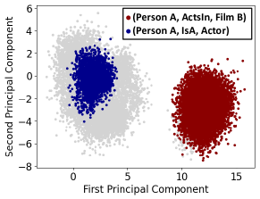
Figure 3: Embedding vectors of base-level triplets in $\langle T_{i}$, ImpliesProfession, $T_{j}\rangle$ where $T_{i}$ is (Person A, ActsIn, Film B) and $T_{j}$ is (Person A, IsA, Actor) in FBH. Both ${\bf{T}}_{i}$ and ${\bf{T}}_{j}$ embedding vectors from BiVE are well-clustered.

Triplet Prediction

While BiVE solves a triplet prediction problem using the scoring function $F_{\text{tp}}(X)$, none of the baseline methods can deal with the higher-level triplets. To feed the higher-level triplets to the baseline methods, we create a new knowledge graph $G_{T}$ where a base-level triplet is converted into an entity and a higher-level triplet is converted into a triplet. Let $T_{i}=(h_{i},r_{i},t_{i})\in\mathcal{E}_{\text{train}}$ denote a base-level triplet. We define $G_{T}\coloneqq(\mathcal{E}_{\text{train}},\widehat{\mathcal{R}},\mathcal{H}_{\text{train}})$, where each $T_{i}$ is considered as an entity. If we train the baseline methods using $G_{T}$, the triplet prediction task can be considered as a link prediction problem on $G_{T}$. However, in this case, it is not guaranteed that all $T_{i}$ involved in the triplets in $\mathcal{H}_{\text{test}}$ appear in $\mathcal{H}_{\text{train}}$ because we randomly split $\mathcal{H}$ into training, validation, and test sets. Therefore, for the baseline methods, the problem becomes an inductive setting instead of a transductive setting. Indeed, among the baseline methods, Neural-LP and DRUM are inductive methods and we include these methods because they can conduct inductive inference. We assume that the candidates of a triplet prediction problem should be included in the training set of the base-level knowledge graph, which aligns with a realistic setting. By taking into account both the base-level knowledge graph and the higher-level triplets simultaneously, the problem becomes a transductive setting for BiVE. This shows that simply converting the higher-level triplets into $G_{T}$ cannot replace our model.

Table 3 shows the results of triplet prediction. We see that BiVE-Q and BiVE-B significantly outperform all other state-of-the-art baseline methods in terms of all the three metrics on all three real-world datasets. Note that the number of candidates of a triplet prediction problem is equal to the number of base-level triplets in $\mathcal{E}_{\text{train}}$. Therefore, achieving the MR of 18.7 on FBH, for example, is surprising because we have 248,095 candidates in $\mathcal{E}_{\text{train}}$. We visualize the embedding vectors generated by BiVE-Q on FBH in Figure 3. We take all higher-level triplets in the form of $\langle T_{i}$, ImpliesProfession, $T_{j}\rangle$ and visualize the embedding vectors of $T_{i}$ and $T_{j}$ using Principal Component Analysis. In Figure 3, we only highlight the base-level triplets $T_{i}$ and $T_{j}$ where $T_{i}$ is (Person A, ActsIn, Film B) and $T_{j}$ is (Person A, IsA, Actor). We see that both ${\bf{T}}_{i}$ and ${\bf{T}}_{j}$ embedding vectors are well-clustered, meaning that BiVE generates embeddings by appropriately reflecting the structure of the higher-level triplets.

	FBH			FBHE			DBHE
	MR ($\downarrow$)	MRR ($\uparrow$)	Hit@10 ($\uparrow$)	MR ($\downarrow$)	MRR ($\uparrow$)	Hit@10 ($\uparrow$)	MR ($\downarrow$)	MRR ($\uparrow$)	Hit@10 ($\uparrow$)
ASER	1183.9$\pm$0.0	0.251$\pm$0.000	0.316$\pm$0.000	970.7$\pm$0.0	0.289$\pm$0.000	0.382$\pm$0.000	1893.5$\pm$0.0	0.225$\pm$0.000	0.348$\pm$0.000
MINERVA	3817.8$\pm$58.9	0.328$\pm$0.013	0.415$\pm$0.009	3018.5$\pm$45.8	0.407$\pm$0.013	0.492$\pm$0.014	2934.1$\pm$32.2	0.362$\pm$0.007	0.433$\pm$0.014
Multi-Hop	1878.2$\pm$12.0	0.421$\pm$0.003	0.578$\pm$0.003	1447.3$\pm$11.9	0.443$\pm$0.002	0.615$\pm$0.002	1012.3$\pm$28.5	0.442$\pm$0.007	0.652$\pm$0.008
Neural-LP	185.9$\pm$1.3	0.433$\pm$0.002	0.648$\pm$0.004	146.2$\pm$1.0	0.466$\pm$0.002	0.716$\pm$0.007	32.2$\pm$1.9	0.517$\pm$0.006	0.756$\pm$0.004
DRUM	262.7$\pm$13.3	0.394$\pm$0.002	0.555$\pm$0.003	207.6$\pm$10.0	0.413$\pm$0.010	0.620$\pm$0.018	49.0$\pm$3.9	0.470$\pm$0.010	0.732$\pm$0.012
AnyBURL	228.5$\pm$11.8	0.380$\pm$0.004	0.563$\pm$0.013	166.0$\pm$7.9	0.418$\pm$0.002	0.607$\pm$0.008	81.7$\pm$4.0	0.403$\pm$0.002	0.594$\pm$0.004
PTransE	214.8$\pm$0.7	0.440$\pm$0.001	0.686$\pm$0.002	167.0$\pm$1.8	0.516$\pm$0.001	0.752$\pm$0.001	19.3$\pm$0.2	0.505$\pm$0.004	0.780$\pm$0.001
RPJE	212.5$\pm$0.1	0.440$\pm$0.001	0.686$\pm$0.001	159.0$\pm$0.0	0.528$\pm$0.001	0.753$\pm$0.001	19.3$\pm$0.1	0.504$\pm$0.004	0.779$\pm$0.002
TransD	190.1$\pm$18.0	0.300$\pm$0.003	0.496$\pm$0.005	165.6$\pm$8.0	0.363$\pm$0.003	0.529$\pm$0.006	35.5$\pm$1.0	0.436$\pm$0.006	0.708$\pm$0.005
ANALOGY	341.0$\pm$218.7	0.182$\pm$0.065	0.291$\pm$0.125	113.3$\pm$2.0	0.409$\pm$0.004	0.581$\pm$0.004	279.1$\pm$197.1	0.140$\pm$0.089	0.253$\pm$0.166
QuatE	163.7$\pm$3.6	0.346$\pm$0.006	0.494$\pm$0.011	1546.4$\pm$98.0	0.124$\pm$0.022	0.189$\pm$0.014	551.6$\pm$40.5	0.208$\pm$0.013	0.309$\pm$0.023
BiQUE	111.0$\pm$0.9	0.423$\pm$0.002	0.641$\pm$0.002	90.1$\pm$0.5	0.387$\pm$0.009	0.617$\pm$0.011	29.5$\pm$1.2	0.378$\pm$0.007	0.677$\pm$0.004
BiVE-Q	7.0$\pm$0.3	0.752$\pm$0.005	0.906$\pm$0.002	11.0$\pm$0.3	0.698$\pm$0.004	0.839$\pm$0.003	12.5$\pm$1.0	0.606$\pm$0.009	0.828$\pm$0.010
BiVE-B	6.6$\pm$0.3	0.762$\pm$0.007	0.911$\pm$0.002	12.8$\pm$0.4	0.696$\pm$0.005	0.834$\pm$0.002	3.2$\pm$0.1	0.801$\pm$0.003	0.958$\pm$0.002

Table 4: Results of Conditional Link Prediction. The best scores are boldfaced and the second best scores are underlined. Our models, BiVE-Q and BiVE-B, significantly outperform all baseline methods in terms of all metrics on all datasets.

Problem		Prediction by BiVE-Q
$\langle$(?, HasAFriendshipWith, Kelly_Preston), EquivalentTo, (Kelly_Preston, HasAFriendshipWith, George_Clooney)$\rangle$		George_Clooney
1-3 $\langle$(?, HasAFriendshipWith, Kelly_Preston), EquivalentTo, (Kelly_Preston, HasAFriendshipWith, Tom_Cruise)$\rangle$		Tom_Cruise
$\langle$(Joe_Jonas, IsA, ?), ImpliesProfession, (Joe_Jonas, IsA, Actor)$\rangle$		Voice_Actor
1-3 $\langle$(Joe_Jonas, IsA, ?), ImpliesProfession, (Joe_Jonas, IsA, Musician)$\rangle$		Singer-songwriter
$\langle$(Bucknell_University, HasAHeadquarterIn, Pennsylvania), ImpliesLocation, (?, Contains, Bucknell_University)$\rangle$		Pennsylvania
1-3 $\langle$(Bucknell_University, HasAHeadquarterIn, United_States), ImpliesLocation, (?, Contains, Bucknell_University)$\rangle$		United_States
$\langle$(Saturn_Award_for_Best_Director, Nominates, Avatar), PrerequisiteFor, (Avatar, Wins, ?)$\rangle$		Saturn_Award_for_Best_Director
1-3 $\langle$(Academy_Award_for_Best_Visual_Effects, Nominates, Avatar), PrerequisiteFor, (Avatar, Wins, ?)$\rangle$		Academy_Award_for_Best_Visual_Effects

Table 5: Examples of Conditional Link Prediction on FBHE. BiVE correctly predicts the answers for all the above problems.

	FBHE		DBHE
	MR ($\downarrow$)	Hit@10 ($\uparrow$)	MR ($\downarrow$)	Hit@10 ($\uparrow$)
ASER	1489.3$\pm$0.0	0.323$\pm$0.000	2218.8$\pm$0.0	0.197$\pm$0.000
MINERVA	3828.4$\pm$56.9	0.339$\pm$0.003	3530.7$\pm$50.1	0.297$\pm$0.006
Multi-Hop	2284.0$\pm$9.5	0.500$\pm$0.001	2489.4$\pm$15.3	0.404$\pm$0.004
Neural-LP	1942.5$\pm$0.5	0.486$\pm$0.001	2904.8$\pm$0.6	0.357$\pm$0.001
DRUM	1945.6$\pm$0.8	0.490$\pm$0.002	2904.7$\pm$0.7	0.359$\pm$0.001
AnyBURL	342.0$\pm$4.6	0.526$\pm$0.002	879.1$\pm$5.7	0.364$\pm$0.003
PTransE	2077.6$\pm$10.3	0.333$\pm$0.000	3346.0$\pm$20.0	0.277$\pm$0.002
RPJE	1754.6$\pm$7.5	0.368$\pm$0.001	2991.7$\pm$28.1	0.341$\pm$0.000
TransD	166.3$\pm$1.3	0.527$\pm$0.001	429.0$\pm$7.5	0.423$\pm$0.001
ANALOGY	227.3$\pm$8.3	0.486$\pm$0.002	621.5$\pm$20.9	0.323$\pm$0.008
QuatE	139.0$\pm$1.6	0.581$\pm$0.001	409.6$\pm$8.5	0.440$\pm$0.001
BiQUE	134.9$\pm$0.9	0.583$\pm$0.001	376.6$\pm$3.5	0.446$\pm$0.002
BiVE-Q	125.2$\pm$0.9	0.584$\pm$0.001	405.4$\pm$4.1	0.438$\pm$0.002
BiVE-B	123.5$\pm$1.0	0.586$\pm$0.001	377.3$\pm$6.7	0.444$\pm$0.001

Table 6: Results of Base-Level Link Prediction.

Conditional Link Prediction

To solve a conditional link prediction problem, BiVE uses the scoring function $F_{\text{clp}}(x)$. On the other hand, the baseline methods cannot directly solve the conditional link prediction problem. To allow the baseline methods to solve $\langle T_{i},\widehat{r},(h_{j},r_{j},?)\rangle$, we define a scoring function of the baseline methods as follows: $F(x)\coloneqq f({\bf{h}}_{j},{\bf{r}}_{j},{\bf{x}})+f({\bf{T}}_{i},{\bf{\widehat{r}}},z(h_{j},r_{j},x))$ for all $x\in\mathcal{V}$ where the former is computed on the original base-level knowledge graph, the latter is computed on $G_{T}$, $z(h_{j},r_{j},x)$ returns an embedding vector of $(h_{j},r_{j},x)$, and $f(\cdot)$ is the scoring function of each baseline method. We cannot get $f({\bf{T}}_{i},{\bf{\widehat{r}}},z(h_{j},r_{j},x))$ if $(h_{j},r_{j},x)\notin\mathcal{E}_{\text{train}}$. In that case, we compute the score using the randomly initialized vectors in PTransE, RPJE, TransD, ANALOGY, QuatE, and BiQUE, whereas we set $f({\bf{T}}_{i},{\bf{\widehat{r}}},z(h_{j},r_{j},x))=0$ for the other baseline methods by considering the mechanisms of how each of the baseline methods assigns scores. In Table 4, BiVE-Q and BiVE-B significantly outperform all other baseline methods in conditional link prediction on all three real-world datasets. In Table 5, we show some example problems of conditional link prediction in FBHE and the predictions made by BiVE-Q where it correctly predicts the answers. When we consider a problem in the form of $\langle T_{i},\widehat{r},(h_{j},r_{j},?)\rangle$, even though we have the same problem of $(h_{j},r_{j},?)$, the answer becomes different depending on $T_{i}$. This is the difference between the typical base-level link prediction and the conditional link prediction.

	Relation Sequence $p_{k}$	Relation $r$	$c(p_{k},r)$	$|S_{kr}|$	Examples of the Augmented Triplets
FBHE	NominatesIn, $\mbox{NominatesIn}^{-1}$, ActsIn, ImpliesProfession, IsA	IsA	0.86	610	(Patty_Duke, IsA, Actor)
	ParticipatesIn, $\mbox{ParticipatesIn}^{-1}$, ImpliesSports, $\mbox{Plays}^{-1}$, ParticipatesIn	ParticipatesIn	0.81	57	(Houston_Rockets, ParticipatesIn, 2003_NBA_Draft)
	Plays, $\mbox{Plays}^{-1}$, $\mbox{{ImpliesSports}}^{-1}$, HasPosition	HasPosition	0.78	295	(Bayer_04_Leverkusen, HasPosition, Forward)
	Contains, $\mbox{Contains}^{-1}$, $\mbox{{ImpliesLocation}}^{-1}$, HasAHeadquarterIn	Contains	0.72	81	(United_States, Contains, Charlottesville_Virginia)
	$\mbox{Program}^{-1}$, Program, Language	Language	0.70	148	(David_Copperfield_(Film), Language, English_Language)
1-6 DBHE	Genre, $\mbox{{ImpliesGenre}}^{-1}$, Genre, $\mbox{Genre}^{-1}$, $\mbox{{ImpliesGenre}}^{-1}$, Genre	Genre	0.78	120	(Kenny_Rogers, Genre, Pop_Rock)
	IsPartOf, IsPartOf, ImpliesLocation, IsPartOf	IsPartOf	0.76	69	(San_Pedro_Los_Angeles, IsPartOf, California)
	IsPartOf, $\mbox{IsPartOf}^{-1}$, $\mbox{{ImpliesLocation}}^{-1}$, $\mbox{IsPartOf}^{-1}$, TimeZone	TimeZone	0.75	122	(Brockton_Massachusetts, TimeZone, Eastern_Time_Zone)
	$\mbox{IsProducedBy}^{-1}$, IsProducedBy, ImpliesProfession, IsA	IsA	0.73	80	(Jim_Wilson, IsA, Film_Producer)
	Region, $\mbox{Region}^{-1}$, Country	Country	0.70	41	(Pontefract, Country, England)

Table 7: Examples of the Augmented Triplets in FBHE and DBHE. The higher-level relations are boldfaced.

	FBH	FBHE	DBHE
No. of unique $(p_{k},r)$	340,194	349,120	149,365
No. of $(p_{k},r)$ with $c(p_{k},r)\geq 0.7$	35,803	39,727	7,030
No. of augmented triplets	16,601	17,463	2,026
$|\mathcal{S}\cap\mathcal{E}_{\text{valid}}|+|\mathcal{S}\cap\mathcal{E}_{\text{test}}|$	5,237	5,380	316

Table 8: Statistics of the Augmented Triplets.

		FBH	FBHE	DBHE
TP	$L_{\text{base}}+L_{\text{high}}$	19.2	28.1	65.4
	$L_{\text{base}}+L_{\text{high}}+L_{\text{aug}}$	18.7	33.1	56.6
1-5 CLP	$L_{\text{base}}+L_{\text{high}}$	8.3	12.5	12.4
	$L_{\text{base}}+L_{\text{high}}+L_{\text{aug}}$	7.0	11.0	12.5
1-5 BLP	$L_{\text{base}}$	139.0	139.0	409.6
	$L_{\text{base}}+L_{\text{high}}$	138.4	138.4	408.1
	$L_{\text{base}}+L_{\text{aug}}$	124.7	125.2	404.9
	$L_{\text{base}}+L_{\text{high}}+L_{\text{aug}}$	124.7	125.2	405.4

Table 9: Ablation study of BiVE with different combinations of the loss terms. The average MR scores on triplet prediction (TP), conditional link prediction (CLP), and the base-level link prediction (BLP).

		Triplet Prediction			Conditional LP
$\widehat{r}$	Freq.	MR	MRR	Hit@10	MR	MRR	Hit@10
EquivalentTo	98	17.5	0.416	0.679	2.2	0.744	0.977
ImpliesLanguage	29	35.6	0.292	0.578	18.4	0.632	0.786
ImpliesProfession	210	71.3	0.427	0.569	11.5	0.704	0.844
ImpliesLocation	163	42.2	0.219	0.463	9.4	0.502	0.816
ImpliesTimeZone	44	20.6	0.354	0.631	17.8	0.604	0.707
ImpliesGenre	84	113.8	0.177	0.345	32.6	0.408	0.681
NextAlmaMater	14	71.0	0.161	0.379	2.5	0.651	0.971
TransfersTo	29	67.0	0.140	0.374	5.7	0.527	0.537

Table 10: Performance of BiVE per higher-level relation in DBHE. Freq. indicates the number of higher-level triplets in $\mathcal{H}_{\text{test}}$ associated with $\widehat{r}$.

Base-Level Link Prediction

We present the performance of the typical base-level link prediction in Table 6. Since the base-level knowledge graphs of FBH and FBHE are identical, the performance of all baseline methods is the same on FBH and FBHE. The base-level link prediction performance of BiVE on FBH and FBHE is also very similar to each other. We observed that the MRR scores of our BiVE models and the two best baselines are almost the same on FBHE and DBHE. On FBHE, the average MRR scores of BiVE-Q and QuatE are both 0.354, and those of BiVE-B and BiQUE are both 0.356. On DBHE, the average MRR score of BiVE-Q is 0.265 and that of QuatE is 0.264; the average MRR score of BiVE-B is 0.275 and that of BiQUE is 0.274. Overall, our BiVE models show comparable results to the baseline methods for the typical link prediction task; our BiVE models have the extra capability of dealing with the triplet prediction and conditional link prediction tasks.

Data Augmentation of BiVE

We analyze the augmented triplets that are added by our data augmentation strategy. In Table 7, we show some examples of a relation sequence $p_{k}$, a relation $r$, and the confidence of $(p_{k},r)$, the number of augmented triplets based on $(p_{k},r)$ denoted by $|\mathcal{S}_{kr}|$, and examples of the augmented triplets in FBHE and DBHE. According to our random walk policy, we do not allow going back to an entity that has already been visited. Thus, even though a relation and its reverse relation are consecutively appeared in a relation sequence in Table 7, it does not mean that we return back to the previous entity; instead, it means that the walk steps another entity adjacent to the corresponding relation. In Table 8, we show statistics of the augmented triplets. Among the diverse combinations of a relation sequence $p_{k}$ and a relation $r$, we consider the $(p_{k},r)$ pairs whose confidence scores are greater than or equal to $0.7$. It is interesting to see that there exist considerable overlaps between the set $\mathcal{S}$ of the augmented triplets and $\mathcal{E}_{\text{valid}}$ and $\mathcal{E}_{\text{test}}$, indicating that our augmented triplets include many ground-truth triplets that are missing in the training set.

Ablation Study of BiVE

In BiVE, we have three different types of loss terms: $L_{\text{base}}$, $L_{\text{high}}$, and $L_{\text{aug}}$. Using different combinations of these loss terms, we measure the performance of BiVE to check the importance of each loss term. Table 9 shows the average MR scores of BiVE-Q with different combinations of the loss terms in three tasks: triplet prediction (TP), conditional link prediction (CLP), and base-level link prediction (BLP). Note that TP and CLP require at least two terms, $L_{\text{base}}$ and $L_{\text{high}}$. Also, Table 10 shows the performance of BiVE-Q per higher-level relation in DBHE, where Freq. indicates the number of higher-level triplets in $\mathcal{H}_{\text{test}}$ associated with $\widehat{r}$. Among the eight higher-level relations in DBHE, NextAlmaMater and TransfersTo require externally-sourced knowledge. While EquivalentTo is the easiest one, the performance on the other higher-level relations varies depending on the tasks and the metrics.

Conclusion and Future Work

We define a bi-level knowledge graph by introducing the higher-level relationships between triplets. We propose BiVE, which takes into account the structures of the base-level triplets, the higher-level triplets, and the augmented triplets. Experimental results show that BiVE significantly outperforms state-of-the-art methods in terms of the two newly defined tasks: triplet prediction and conditional link prediction. We believe our method can contribute to advancing many knowledge-based applications, including conditional QA [33] and multi-hop QA [9], with a special emphasis on mixing a neural language model and structured knowledge [40].

We plan to analyze the pros and cons of our bi-level knowledge graphs and compare them with other forms of extended knowledge graphs, such as hyper-relational knowledge graphs [5]. Also, we will extend BiVE and the proposed tasks to an inductive learning scenario where both entities and relations can be new at inference time [22].

Appendix

Experimental Settings

All experiments are conducted on machines equipped with Intel(R) Xeon(R) E5-2690 v4 CPUs and 512GB memory. We use RTX A6000 GPUs unless otherwise stated.

Baseline Methods

In experiments, we use 12 different baseline methods which are ASER [41], MINERVA [7], Multi-Hop [24], Neural-LP [39], DRUM [31], AnyBURL [27], PTransE [25], RPJE [29], TransD [16], ANALOGY [26], QuatE [42], and BiQUE [12]. We use GeForce RTX 2080Ti GPUs to run MINERVA, Neural-LP, and DRUM because these methods use TensorFlow version 1.

For ASER, we implement the string matching based inference model described in [41]. The original program of MINERVA is designed only to predict a tail entity. We add reversed triplets to also predict a head entity. In Multi-Hop, we set all the add_reverse_edge options to be true. We run AnyBURL with different rule learning times: 10 seconds, 100 seconds, 1,000 seconds and 10,000 seconds. Since the results of running 10,000 seconds are similar to those of 1,000 seconds, we use the results of 1,000 seconds. We use the best hyperparameters provided by the authors of each of the baseline methods except PTransE, RPJE, TransD, ANALOGY, QuatE, and BiQUE; we tune the hyperparameters of PTransE, RPJE, TransD, ANALOGY, QuatE, and BiQUE because the best hyperparameters are not provided for these methods.

For PTransE and RPJE, we tune the learning rate $\alpha$ using the range of $\alpha=\{10^{-6},5\cdot 10^{-6},10^{-5},5\cdot 10^{-5},10^{-4},5\cdot 10^{-4}\}$ and the margin $\gamma$ using the range of $\gamma=\{0.5,1.0,2.0\}$. We use TransD, ANALOGY, QuatE, and BiQUE, which are implemented based on OpenKE [14]. For TransD, we tune the learning rate $\alpha$ using the range of $\alpha=\{0.1,0.5,1.0,2.0,5.0\}$ and the margin $\gamma$ using the range of $\gamma=\{2.0,5.0,10.0\}$. For ANALOGY, we tune the learning rate $\alpha$ using the range of $\alpha=\{0.001,0.005,0.01,0.05,0.1,0.5\}$ and the regularization rate $\beta$ using the range of $\beta=\{0.1,0.5,1.0\}$. For QuatE and BiQUE, we tune the learning rate $\alpha$ using the range of $\alpha=\{0.1,0.5,1.0,2.0,5.0\}$ and the regularization rate $\beta$ using the range of $\beta=\{0.1,0.5,1.0\}$. For TransD, ANALOGY, QuatE, and BiQUE, validation is done every 50 epochs up to 500 epochs, and we select the best epoch based on the validation results. Table 11 shows the best hyperparameters of these methods for the triplet prediction and the base-level link prediction. For the conditional link prediction problem, we combine the scores of the triplet prediction and the base-level link prediction as described in the main paper; we use the best hyperparameters of the triplet prediction and the base-level link prediction.

		Triplet Prediction	Base-Level Link Prediction
PTransE	FBH	$\alpha=5\cdot 10^{-6},\gamma=0.5$	$\alpha=10^{-6},\gamma=0.5$
	FBHE	$\alpha=5\cdot 10^{-6},\gamma=0.5$	$\alpha=10^{-6},\gamma=0.5$
	DBHE	$\alpha=10^{-6},\gamma=0.5$	$\alpha=10^{-6},\gamma=0.5$
RPJE	FBH	$\alpha=10^{-6},\gamma=1.0$	$\alpha=10^{-6},\gamma=1.0$
	FBHE	$\alpha=10^{-6},\gamma=1.0$	$\alpha=10^{-6},\gamma=1.0$
	DBHE	$\alpha=10^{-6},\gamma=1.0$	$\alpha=10^{-6},\gamma=1.0$
TransD	FBH	$\alpha=0.5,\gamma=5.0$	$\alpha=1.0,\gamma=5.0$
	FBHE	$\alpha=0.1,\gamma=5.0$	$\alpha=1.0,\gamma=5.0$
	DBHE	$\alpha=0.5,\gamma=5.0$	$\alpha=0.1,\gamma=5.0$
ANALOGY	FBH	$\alpha=0.01,\beta=0.01$	$\alpha=0.01,\beta=0.1$
	FBHE	$\alpha=0.01,\beta=0.01$	$\alpha=0.01,\beta=0.1$
	DBHE	$\alpha=0.05,\beta=0.1$	$\alpha=0.01,\beta=0.1$
QuatE	FBH	$\alpha=1.0,\beta=0.05$	$\alpha=0.1,\beta=0.05$
	FBHE	$\alpha=1.0,\beta=0.01$	$\alpha=0.1,\beta=0.05$
	DBHE	$\alpha=0.5,\beta=0.05$	$\alpha=0.5,\beta=0.1$
BiQUE	FBH	$\alpha=0.1,\beta=0.01$	$\alpha=0.5,\beta=0.05$
	FBHE	$\alpha=0.1,\beta=0.01$	$\alpha=0.5,\beta=0.05$
	DBHE	$\alpha=0.1,\beta=0.05$	$\alpha=0.5,\beta=0.1$

Table 11: The best hyperparameters of PTransE, RPJE, TransD, ANALOGY, QuatE, and BiQUE. $\alpha,\beta,\gamma$ indicate the learning rate, the regularization rate, and the margin, respectively.

Hyperparameters of BiVE

Within BiVE, we use the scoring function of QuatE [42] for BiVE-Q and BiQUE [12] for BiVE-B. On the validation set, we tune the learning rate $\alpha$, the regularization rate $\beta$, and the weights $\lambda_{1}$ and $\lambda_{2}$ in $L_{\text{{BiVE}}}$. We use the search space of $\{0.2,0.5,1.0\}$ for both $\lambda_{1}$ and $\lambda_{2}$. Validation is done every 50 epochs up to 500 epochs, and we select the best epoch based on the validation results. Table 12 shows the best hyperparameters of BiVE on the validation sets.

		FBH				FBHE				DBHE
		$\alpha$	$\beta$	$\lambda_{1}$	$\lambda_{2}$	$\alpha$	$\beta$	$\lambda_{1}$	$\lambda_{2}$	$\alpha$	$\beta$	$\lambda_{1}$	$\lambda_{2}$
BiVE-Q	Triplet Prediction	0.1	0.01	0.5	1.0	0.1	0.01	1.0	0.2	0.5	0.05	0.2	1.0
	Conditional Link Prediction	0.1	0.01	1.0	0.2	0.1	0.01	1.0	0.2	0.5	0.01	1.0	0.2
	Base-Level Link Prediction	0.1	0.05	1.0	0.2	0.1	0.05	0.5	0.2	0.5	0.1	0.5	0.2
BiVE-B	Triplet Prediction	0.1	0.01	0.5	0.5	0.1	0.01	0.5	0.2	0.1	0.01	1.0	0.2
	Conditional Link Prediction	0.1	0.01	1.0	0.2	0.1	0.01	1.0	0.2	0.5	0.01	1.0	0.2
	Base-Level Link Prediction	0.1	0.05	0.5	0.2	0.1	0.05	0.5	0.5	0.5	0.1	0.2	1.0

Table 12: The best hyperparameters of BiVE on validation.

Real-World Bi-Level Knowledge Graphs

We describe the details about how we create the three real-world bi-level knowledge graphs, FBH, FBHE, and DBHE.

Base-Level Knowledge Graphs

We use FB15K237 [34] as the base-level knowledge graphs for FBH and FBHE. FB15K237 is a standard benchmark knowledge graph dataset which is constructed by taking 401 most frequent relations and merging near-duplicate and inverse relations in FB15K [3] from Freebase [2].

We use a filtered version of DB15K [11] which is constructed based on DBpedia [1]. By following the strategy used in [38], we first remove the relations that are not in the form of DBpedia URL, such as ‘http://www.w3.org/2000/01/rdf-schema#seeAlso’, since these types of relations do not have clear semantics. Then, we take the relations involved in more than 100 triplets and merge near-duplicate and inverse relations by following the strategy used in [34]. For example, (Chevrolet, owningCompany, General_Motors) and (Chevrolet, owner, General_Motors) are merged.

Higher-Level Triplets

In Table 13, we show the higher-level relations and the corresponding examples of the higher-level triplets used to create FBH, FBHE, and DBHE. While FBHE contains all ten higher-level relations, FBH contains only the first six higher-level relations.

Among the higher-level relations in Table 13, WorksFor, SucceededBy, TransfersTo, and HigherThan in FBHE and NextAlmaMater and TransfersTo in DBHE require externally-sourced knowledge. For example, we crawled Wikipedia articles to find information about the (vice)presidents of the United States, the teams a player was playing for, and the alma mater of politicians. Also, to create $\langle T_{i}$, HigherThan, $T_{j}\rangle$ in FBHE, we used the most recent rankings of Fortune 1000 and Times University Ranking. Table 14 and Table 15 show all types of higher-level triplets used to create FBH, FBHE, and DBHE.

	$\widehat{r}$	$\langle T_{i},\widehat{r},T_{j}\rangle$	Description
FBHE	PrerequisiteFor	$T_{i}$: (BAFTA_Award, Nominates, The_King’s_Speech)	For The King’s Speech to win BAFTA Award, BAFTA Award should nominate The
		$T_{j}$: (The_King’s_Speech, Wins, BAFTA_Award)	King’s Speech.
2-4	EquivalentTo	$T_{i}$: (Hillary_Clinton, IsMarriedTo, Bill_Clinton)	The two triplets indicate the same information.
		$T_{j}$: (Bill_Clinton, IsMarriedTo, Hillary_Clinton)
2-4	ImpliesLocation	$T_{i}$: (Sweden, CapitalIsLocatedIn, Stockholm)	‘The capital of Sweden is Stockholm’ implies ‘Sweden contains Stockholm’.
		$T_{j}$: (Sweden, Contains, Stockholm)
2-4	ImpliesProfession	$T_{i}$: (Liam_Neeson, ActsIn, Love_Actually)	‘Liam Neeson acts in Love Actually’ implies ‘Liam Neeson is an actor’.
		$T_{j}$: (Liam_Neeson, IsA, Actor)
2-4	ImpliesSports	$T_{i}$: (Boston_Red_Socks, HasPosition, Infield)	‘Boston Red Socks has an infield position’ implies ‘Boston Red Socks plays baseball’.
		$T_{j}$: (Boston_Red_Socks, Plays, Baseball)
2-4	NextEventPlace	$T_{i}$: (1932_Summer_Olympics, IsHeldIn, Los_Angeles)	Summer Olympics in 1932 and 1936 were held in Los Angeles and Berlin, respectively.
		$T_{j}$: (1936_Summer_Olympics, IsHeldIn, Berlin)	1936 Summer Olympics is the next event of 1932 Summer Olympics.
2-4	WorksFor	$T_{i}$: (Joe_Biden, HoldsPosition, Vice_President)	Joe Biden was a vice president when Barack Obama was a president of the United States.
		$T_{j}$: (Barack_Obama, HoldsPosition, President)
2-4	SucceededBy	$T_{i}$: (George_W._Bush, HoldsPosition, President)	President Barack Obama succeeded President George W. Bush.
		$T_{j}$: (Barack_Obama, HoldsPosition, President)
2-4	TransfersTo	$T_{i}$: (David_Beckham, PlaysFor, Real_Madrid_CF)	David Beckham transferred from Real Madrid CF to LA Galaxy.
		$T_{j}$: (David_Beckham, PlaysFor, LA_Galaxy)
2-4	HigherThan	$T_{i}$: (Walmart, IsRankedIn, Fortune_500)	Walmart is ranked higher than Bank of America in Fortune 500.
		$T_{j}$: (Bank_of_America, IsRankedIn, Fortune_500)
1-4 DBHE	EquivalentTo	$T_{i}$: (David_Beckham, IsMarriedTo, Victoria_Beckham)	The two triplets indicate the same information.
		$T_{j}$: (Victoria_Beckham, IsMarriedTo, David_Beckham)
2-4	ImpliesLanguage	$T_{i}$: (Italy, HasOfficialLanguage, Italian_Language)	‘The official language of Italy is the Italian language’ implies ‘The Italian language is
		$T_{j}$: (Italy, UsesLanguage, Italian_Language)	used in Italy’.
2-4	ImpliesProfession	$T_{i}$: (Psycho, IsDirectedBy, Alfred_Hitchcock)	‘Psycho is directed by Alfred Hitchcock’ implies ‘Alfred Hitchcock is a film producer’.
		$T_{j}$: (Alfred_Hitchcock, IsA, Film_Producer)
2-4	ImpliesLocation	$T_{i}$: (Mariah_Carey, LivesIn, New_York_City)	‘Mariah Carey lives in New York City’ implies ‘Mariah Carey lives in New York’
		$T_{j}$: (Mariah_Carey, LivesIn, New_York)
2-4	ImpliesTimeZone	$T_{i}$: (Czech_Republic, TimeZone, Central_European)	‘Czech Republic is included in Central European Time Zone’ implies ‘Prague is included
		$T_{j}$: (Prague, TimeZone, Central_European)	in Central European Time Zone’.
2-4	ImpliesGenre	$T_{i}$: (Pharrell_Williams, Genre, Progressive_Rock)	‘Pharrell Williams is a progressive rock musician’ implies ‘Pharrell Williams is a rock
		$T_{j}$: (Pharrell_Williams, Genre, Rock_Music)	musician’.
2-4	NextAlmaMater	$T_{i}$: (Gerald_Ford, StudiesIn, University_of_Michigan)	Gerald Ford studied in University of Michigan. Then, he studied in Yale University.
		$T_{j}$: (Gerald_Ford, StudiesIn, Yale_University)
2-4	TransfersTo	$T_{i}$: (Ronaldo, PlaysFor, FC_Barcelona)	Ronaldo transferred from FC Barcelona to Inter Millan.
		$T_{j}$: (Ronaldo, PlaysFor, Inter_Millan)

Table 13: The higher-level relations and the corresponding examples of the higher-level triplets used to create FBHE, and DBHE.

		Example	Frequency
$\langle T_{i}$, PrerequisiteFor, $T_{j}\rangle$	$T_{i}$: (Person A, DatesWith, Person B)	(Bruce_Willis, DatesWith, Demi_Moore)	222
	$T_{j}$: (Person A, BreaksUpWith, Person B)	(Bruce_Willis, BreaksUpWith, Demi_Moore)
2-4	$T_{i}$: (Award A, Nominates, Work B)	(BAFTA_Award, Nominates, The_King’s_Speech)	2,335
	$T_{j}$: (Work B, Wins, Award A)	(The_King’s_Speech, Wins, BAFTA_Award)
2-4	$T_{i}$: (Person A, HasNationality, Country B)	(Neymar, HasNationality, Brazil)	109
	$T_{j}$: (Person A, PlaysFor, National Team of B)	(Neymar, PlaysFor, Brazil_National_Football_Team)
1-4 $\langle T_{i}$, EquivalentTo, $T_{j}\rangle$	$T_{i}$: (Person A, IsASiblingTo, Person B)	(Serena_Williams, IsASiblingTo, Venus_Williams)	120
	$T_{j}$: (Person B, IsASiblingTo, Person A)	(Venus_Williams, IsASiblingTo, Serena_Williams)
2-4	$T_{i}$: (Person A, IsMarriedTo, Person B)	(Hillary_Clinton, IsMarriedTo, Bill_Clinton)	352
	$T_{j}$: (Person B, IsMarriedTo, Person A)	(Bill_Clinton, IsMarriedTo, Hillary_Clinton)
2-4	$T_{i}$: (Person A, HasAFriendshipWith, Person B)	(Bob_Dylan, HasAFriendshipWith, The_Beatles)	1,832
	$T_{j}$: (Person B, HasAFriendshipWith, Person A)	(The_Beatles, HasAFriendshipWith, Bob_Dylan)
2-4	$T_{i}$: (Person A, IsAPeerOf, Person B)	(Jimi_Hendrix, IsAPeerOf, Eric_Clapton)	132
	$T_{j}$: (Person B, IsAPeerOf, Person A)	(Eric_Clapton, IsAPeerOf, Jimi_Hendrix)
1-4 $\langle T_{i}$, ImpliesLocation, $T_{j}\rangle$	$T_{i}$: (Location A, Contains, Location B)	(England, Contains, Warwickshire)	2,415
	$T_{j}$: (Location containing A, Contains, Location in B)	(United_Kingdom, Contains, Birmingham)
2-4	$T_{i}$: (Organization A, Headquarter, Location B)	(Kyoto_University, Headquarter, Kyoto)	820
	$T_{j}$: (Location B, Contains, Organization A)	(Kyoto, Contains, Kyoto_University)
2-4	$T_{i}$: (Country A, CapitalIsLocatedIn, City B)	(Sweden, CapitalIsLocatedIn, Stockholm)	83
	$T_{j}$: (Country A, Contains, City B)	(Sweden, Contains, Stockholm)
1-4 $\langle T_{i}$, ImpliesProfession, $T_{j}\rangle$	$T_{i}$: (Person A, IsA, Specialized Profession of B)	(Mariah_Carey, IsA, Singer-songwriter)	2,364
	$T_{j}$: (Person A, IsA, Profession B)	(Mariah_Carey, IsA, Musician)
2-4	$T_{i}$: (Rock&Roll Hall of Fame, Inducts, Person A)	(Rock&Roll_Hall_of_Fame, Inducts, Bob_Dylan)	66
	$T_{j}$: (Person A, IsA, Musician/Artist)	(Bob_Dylan, IsA, Musician)
2-4	$T_{i}$: (Film A, IsWrittenBy, Person B)	(127_Hours, IsWrittenBy, Danny_Boyle)	893
	$T_{j}$: (Person B, IsA, Writer/Film Producer)	(Danny_Boyle, IsA, Film_producer)
2-4	$T_{i}$: (Person A, ActsIn, Film B)	(Liam_Neeson, ActsIn, Love_Actually)	10,864
	$T_{j}$: (Person A, IsA, Actor)	(Liam_Neeson, IsA, Actor)
2-4	$T_{i}$: (Person A, HoldsPosition, Government Position B)	(Barack_Obama, HoldsPosition, President)	120
	$T_{j}$: (Person A, IsA, Politician)	(Barack_Obama, IsA, Politician)
1-4 $\langle T_{i}$, ImpliesSports, $T_{j}\rangle$	$T_{i}$: (Team A, HasPosition, Position of B)	(Boston_Red_Socks, HasPosition, Infield)	2,936
	$T_{j}$: (Team A, Plays, Sports B)	(Boston_Red_Socks, Plays, Baseball)
2-4	$T_{i}$: (League of A, Includes, Team B)	(National_League, Includes, New_York_Mets)	824
	$T_{j}$: (Team B, Plays, Sports A)	(New_York_Mets, Plays, Baseball)
2-4	$T_{i}$: (Team A, ParticipatesIn, Draft of B)	(Atlanta_Braves, ParticipatesIn, MLB_Draft)	528
	$T_{j}$: (Team A, Plays, Sports B)	(Atlanta_Braves, Plays, Baseball)
1-4 $\langle T_{i}$, NextEventPlace, $T_{j}\rangle$	$T_{i}$: (Event A, IsHeldIn, Location A)	(1932_Summer_Olympics, IsHeldIn, Los_Angeles)	47
	$T_{j}$: (Next Event of A, IsHeldIn, Location B)	(1936_Summer_Olympics, IsHeldIn, Berlin)
1-4 $\langle T_{i}$, WorksFor, $T_{j}\rangle$	$T_{i}$: (Person A, HoldsPosition, Vice President)	(Joe_Biden, HoldsPosition, Vice_President)	13
	$T_{j}$: (Person B, HoldsPosition, President)	(Barack_Obama, HoldsPosition, President)
1-4 $\langle T_{i}$, SucceededBy, $T_{j}\rangle$	$T_{i}$: (Person A, HoldsPosition, President/Vice President)	(George_W._Bush, HoldsPosition, President)	30
	$T_{j}$: (Person B, HoldsPosition, President/Vice President)	(Barack_Obama, HoldsPosition, President)
1-4 $\langle T_{i}$, TransfersTo, $T_{j}\rangle$	$T_{i}$: (Person A, PlaysFor, Team B)	(David_Beckham, PlaysFor, Real_Madrid_CF)	377
	$T_{j}$: (Person A, PlaysFor, Team C)	(David_Beckham, PlaysFor, LA_Galaxy)
1-4 $\langle T_{i}$, HigherThan, $T_{j}\rangle$	$T_{i}$: (Item A, IsRankedIn, Ranking List C)	(Walmart, IsRankedIn, Fortune_500)	7,459
	$T_{j}$: (Item B, IsRankedIn, Ranking List C)	(Bank_of_America, IsRankedIn, Fortune_500)

Table 14: All types of higher-level triplets to create FBH and FBHE.

		Example	Frequency
$\langle T_{i}$, EquivalentTo, $T_{j}\rangle$	$T_{i}$: (Person A, IsMarriedTo, Person B)	(Hillary_Clinton, IsMarriedTo, Bill_Clinton)	314
	$T_{j}$: (Person B, IsMarriedTo, Person A)	(Bill_Clinton, IsMarriedTo, Hillary_Clinton)
2-4	$T_{i}$: (Location A, UsesLanguage, Language B)	(Brazil, UsesLanguage, Portuguese_Language)	120
	$T_{j}$: (Language B, IsSpokenIn, Location A)	(Portuguese_Language, IsSpokenIn, Brazil)
2-4	$T_{i}$: (Person A, Influences, Person B)	(Baruch_Spinoza, Influences, Immanuel_Kant)	394
	$T_{j}$: (Person B, IsInfluencedBy, Person A)	(Immanuel_Kant, IsInfluencedBy, Baruch_Spinoza)
1-4 $\langle T_{i}$, ImpliesLanguage, $T_{j}\rangle$	$T_{i}$: (Location A, HasOfficialLanguage, Language B)	(Italy, HasOfficialLanguage, Italian_Language)	196
	$T_{j}$: (Location A, UsesLanguage, Language B)	(Italy, UsesLanguage, Italian_Language)
2-4	$T_{i}$: (Location A, UsesLanguage, Language B)	(United_States, UsesLanguage, English_Language)	75
	$T_{j}$: (Location in A, UsesLanguage, Language B)	(California, UsesLanguage, English_Language)
1-4 $\langle T_{i}$, ImpliesProfession, $T_{j}\rangle$	$T_{i}$: (Work A, MusicComposedBy, Person B)	(Forrest_Gump, MusicComposedBy, Alan_Silvestri)	553
	$T_{j}$: (Person B, IsA, Musician/Composer)	(Alan_Silvestri, IsA, Composer)
2-4	$T_{i}$: (Work A, Starring, Person B)	(Love_Actually, Starring, Liam_Neeson)	737
	$T_{j}$: (Person B, IsA, Actor)	(Liam_Neeson, IsA, Actor)
2-4	$T_{i}$: (Work A, CinematographyBy, Person B)	(Jurassic_Park, CinematographyBy, Dean_Cundey)	299
	$T_{j}$: (Person B, IsA, Cinematographer)	(Dean_Cundey, IsA, Cinematographer)
2-4	$T_{i}$: (Work A, IsDirectedBy, Person B)	(Psycho, IsDirectedBy, Alfred_Hitchcock)	295
	$T_{j}$: (Person B, IsA, Film_Director/Television_Director)	(Alfred_Hitchcock, IsA, Film_Director)
2-4	$T_{i}$: (Work A, IsProducedBy, Person B)	(King_Kong, IsProducedBy, Merian_C._Cooper)	354
	$T_{j}$: (Person B, IsA, Film_Producer/Television_Producer)	(Merian_C._Cooper, IsA, Film_Producer)
2-4	$T_{i}$: (Person A, AssociatesWithRecordLabel, Record B)	(Bo_Diddley, AssociatesWithRecordLabel, Atlantic_Records)	155
	$T_{j}$: (Person A, IsA, Record_Producer)	(Bo_Diddley, IsA, Record_Producer)
1-4 $\langle T_{i}$, ImpliesLocation, $T_{j}\rangle$	$T_{i}$: (Location A, IsPartOf, Location B)	(Ann_Arbor, IsPartOf, Washtenaw_County_Michigan)	1,174
	$T_{j}$: (Location in A, IsPartOf, Location Containing B)	(Ann_Arbor, IsPartOf, Michigan)
2-4	$T_{i}$: (Organization A, IsLocatedIn, Location B)	(Adobe_Systems, IsLocatedIn, San_Jose_California)	250
	$T_{j}$: (Organization A, IsLocatedIn, Location Containing B)	(Adobe_Systems, IsLocatedIn, California)
2-4	$T_{i}$: (Person A, LivesIn, Location B)	(Mariah_Carey, LivesIn, New_York_City)	213
	$T_{j}$: (Person A, LivesIn, Location Containing B)	(Mariah_Carey, LivesIn, New_York)
1-4 $\langle T_{i}$, ImpliesTimeZone, $T_{j}\rangle$	$T_{i}$: (Location A, TimeZone, Time Zone B)	(Czech_Republic, TimeZone, Central_European_Time)	409
	$T_{j}$: (Location in A, TimeZone, Time Zone B)	(Prague, TimeZone, Central_European_Time)
1-4 $\langle T_{i}$, ImpliesGenre, $T_{j}\rangle$	$T_{i}$: (Musician A, Genre, Genre B)	(Pharrell_Williams, Genre, Progressive_Rock)	767
	$T_{j}$: (Musician A, Genre, Parent Genre of B)	(Pharrell_Williams, Genre, Rock_Music)
1-4 $\langle T_{i}$, NextAlmaMater, $T_{j}\rangle$	$T_{i}$: (Person A, StudiesIn, Institution B)	(Gerald_Ford, StudiesIn, University_of_Michigan)	112
	$T_{j}$: (Person A, StudiesIn, Institution C)	(Gerald_Ford, StudiesIn, Yale_University)
1-4 $\langle T_{i}$, TransfersTo, $T_{j}\rangle$	$T_{i}$: (Person A, PlaysFor, Team B)	(Ronaldo, PlaysFor, FC_Barcelona)	300
	$T_{j}$: (Person A, PlaysFor, Team C)	(Ronaldo, PlaysFor, Inter_Millan)

Table 15: All types of higher-level triplets to create DBHE.

Additional Experimental Results

We provide additional experimental results using a different implementation of BiVE. The implementation of BiVE is based on OpenKE [14]. Three loss functions, $L_{\text{base}}$, $L_{\text{high}}$, and $L_{\text{aug}}$, are implemented based on the Softplus loss provided in OpenKE, which can be formulated as follows:

$$L=\frac{1}{|\mathcal{E}|}\sum_{(h,r,t)\in\mathcal{E}}g(-f({\bf{h}},{\bf{r}},{\bf{t}}))+\frac{1}{|\mathcal{E}^{\prime}|}\sum_{(h^{\prime},r^{\prime},t^{\prime})\in\mathcal{E}^{\prime}}g(f({\bf{h}}^{\prime},{\bf{r}}^{\prime},{\bf{t}}^{\prime}))$$ (1)

We recently implemented a different version of the Softplus loss that averages the loss incurred by the positive and negative triplets at once. The new implementation of the Softplus loss can be formulated as follows:

$$L_{\text{new}}=\frac{1}{|\mathcal{E}|+|\mathcal{E}^{\prime}|}\left[\sum_{(h,r,t)\in\mathcal{E}}g(-f({\bf{h}},{\bf{r}},{\bf{t}}))+\sum_{(h^{\prime},r^{\prime},t^{\prime})\in\mathcal{E}^{\prime}}g(f({\bf{h}}^{\prime},{\bf{r}}^{\prime},{\bf{t}}^{\prime}))\right]$$

Using the new implementation of the loss in BiVE, we provide the experimental results of triplet prediction and conditional link prediction in Table 16 and Table 17. Since ANALOGY, QuatE, and BiQUE also use the Softplus loss implemented in OpenKE, the results of these methods are also changed. We see that the new implementation of the Softplus loss improves the performance of BiVE. Also, Table 18 shows the performance of the typical base-level link prediction. In all experiments, the conclusion remains the same; our BiVE models significantly outperform baseline methods for the triplet prediction and conditional link prediction tasks while achieving comparable results to the baseline methods for the base-level link prediction task. Table 19 shows the results of the ablation study of BiVE with the new implementation.

Note that the original implementation of BiVE is also correct; the loss term defined in (1) aims to make the scores of the positive triplets higher than those of the negative triplets. Both implementations of BiVE can be found at https://github.com/bdi-lab/BiVE.

	FBH			FBHE			DBHE
	MR ($\downarrow$)	MRR ($\uparrow$)	Hit@10 ($\uparrow$)	MR ($\downarrow$)	MRR ($\uparrow$)	Hit@10 ($\uparrow$)	MR ($\downarrow$)	MRR ($\uparrow$)	Hit@10 ($\uparrow$)
ASER	74541.7$\pm$0.0	0.011$\pm$0.000	0.015$\pm$0.000	57916.0$\pm$0.0	0.050$\pm$0.000	0.070$\pm$0.000	18157.6$\pm$0.0	0.042$\pm$0.000	0.075$\pm$0.000
MINERVA	109055.1$\pm$98.5	0.093$\pm$0.002	0.113$\pm$0.002	85571.5$\pm$768.3	0.220$\pm$0.008	0.300$\pm$0.005	20764.3$\pm$72.3	0.177$\pm$0.005	0.221$\pm$0.004
Multi-Hop	108731.7$\pm$43.2	0.105$\pm$0.001	0.117$\pm$0.000	83643.8$\pm$33.2	0.255$\pm$0.012	0.311$\pm$0.003	20505.8$\pm$9.3	0.191$\pm$0.001	0.230$\pm$0.002
Neural-LP	115016.6$\pm$0.0	0.070$\pm$0.000	0.073$\pm$0.000	90000.4$\pm$0.0	0.238$\pm$0.000	0.274$\pm$0.000	21130.5$\pm$0.0	0.170$\pm$0.000	0.209$\pm$0.000
DRUM	115016.6$\pm$0.0	0.069$\pm$0.001	0.073$\pm$0.000	90000.3$\pm$0.0	0.261$\pm$0.000	0.274$\pm$0.000	21130.5$\pm$0.0	0.166$\pm$0.001	0.209$\pm$0.000
AnyBURL	108079.6$\pm$0.0	0.096$\pm$0.000	0.108$\pm$0.000	83136.8$\pm$5.3	0.191$\pm$0.001	0.252$\pm$0.001	20530.8$\pm$0.0	0.177$\pm$0.000	0.214$\pm$0.000
PTransE	111024.3$\pm$855.0	0.069$\pm$0.000	0.071$\pm$0.000	86793.2$\pm$961.0	0.249$\pm$0.001	0.274$\pm$0.000	18888.7$\pm$457.3	0.158$\pm$0.001	0.195$\pm$0.002
RPJE	113082.0$\pm$945.2	0.070$\pm$0.000	0.072$\pm$0.000	89173.1$\pm$797.3	0.267$\pm$0.000	0.274$\pm$0.000	20290.4$\pm$417.2	0.166$\pm$0.001	0.206$\pm$0.002
TransD	74277.3$\pm$2907.8	0.052$\pm$0.001	0.104$\pm$0.002	52159.4$\pm$758.9	0.238$\pm$0.002	0.280$\pm$0.003	16698.1$\pm$370.2	0.116$\pm$0.004	0.189$\pm$0.009
ANALOGY	152635.3$\pm$554.7	0.100$\pm$0.001	0.110$\pm$0.001	118023.1$\pm$337.9	0.284$\pm$0.003	0.310$\pm$0.001	23512.7$\pm$3265.1	0.160$\pm$0.004	0.199$\pm$0.008
QuatE	109954.7$\pm$2068.8	0.104$\pm$0.000	0.114$\pm$0.001	85021.3$\pm$1402.8	0.251$\pm$0.013	0.282$\pm$0.005	27548.3$\pm$304.0	0.163$\pm$0.001	0.191$\pm$0.002
BiQUE	79802.8$\pm$528.9	0.104$\pm$0.000	0.115$\pm$0.000	59997.8$\pm$519.0	0.293$\pm$0.002	0.319$\pm$0.000	18259.8$\pm$231.0	0.160$\pm$0.001	0.194$\pm$0.001
BiVE-Q	5.6$\pm$0.9	0.876$\pm$0.003	0.938$\pm$0.003	10.7$\pm$9.3	0.728$\pm$0.008	0.882$\pm$0.013	4.3$\pm$0.4	0.634$\pm$0.008	0.923$\pm$0.005
BiVE-B	7.9$\pm$1.2	0.862$\pm$0.008	0.931$\pm$0.005	17.7$\pm$23.0	0.708$\pm$0.008	0.863$\pm$0.012	11.6$\pm$5.7	0.629$\pm$0.018	0.867$\pm$0.021

Table 16: Results of Triplet Prediction with New Implementation. The best scores are boldfaced and the second best scores are underlined. Our models, BiVE-Q and BiVE-B, significantly outperform all other baseline methods in terms of all metrics on all datasets.

	FBH			FBHE			DBHE
	MR ($\downarrow$)	MRR ($\uparrow$)	Hit@10 ($\uparrow$)	MR ($\downarrow$)	MRR ($\uparrow$)	Hit@10 ($\uparrow$)	MR ($\downarrow$)	MRR ($\uparrow$)	Hit@10 ($\uparrow$)
ASER	1183.9$\pm$0.0	0.251$\pm$0.000	0.316$\pm$0.000	970.7$\pm$0.0	0.289$\pm$0.000	0.382$\pm$0.000	1893.5$\pm$0.0	0.225$\pm$0.000	0.348$\pm$0.000
MINERVA	3817.8$\pm$58.9	0.328$\pm$0.013	0.415$\pm$0.009	3018.5$\pm$45.8	0.407$\pm$0.013	0.492$\pm$0.014	2934.1$\pm$32.2	0.362$\pm$0.007	0.433$\pm$0.014
Multi-Hop	1878.2$\pm$12.0	0.421$\pm$0.003	0.578$\pm$0.003	1447.3$\pm$11.9	0.443$\pm$0.002	0.615$\pm$0.002	1012.3$\pm$28.5	0.442$\pm$0.007	0.652$\pm$0.008
Neural-LP	185.9$\pm$1.3	0.433$\pm$0.002	0.648$\pm$0.004	146.2$\pm$1.0	0.466$\pm$0.002	0.716$\pm$0.007	32.2$\pm$1.9	0.517$\pm$0.006	0.756$\pm$0.004
DRUM	262.7$\pm$13.3	0.394$\pm$0.002	0.555$\pm$0.003	207.6$\pm$10.0	0.413$\pm$0.010	0.620$\pm$0.018	49.0$\pm$3.9	0.470$\pm$0.010	0.732$\pm$0.012
AnyBURL	228.5$\pm$11.8	0.380$\pm$0.004	0.563$\pm$0.013	166.0$\pm$7.9	0.418$\pm$0.002	0.607$\pm$0.008	81.7$\pm$4.0	0.403$\pm$0.002	0.594$\pm$0.004
PTransE	214.8$\pm$0.7	0.440$\pm$0.001	0.686$\pm$0.002	167.0$\pm$1.8	0.516$\pm$0.001	0.752$\pm$0.001	19.3$\pm$0.2	0.505$\pm$0.004	0.780$\pm$0.001
RPJE	212.5$\pm$0.1	0.440$\pm$0.001	0.686$\pm$0.001	159.0$\pm$0.0	0.528$\pm$0.001	0.753$\pm$0.001	19.3$\pm$0.1	0.504$\pm$0.004	0.779$\pm$0.002
TransD	190.1$\pm$18.0	0.300$\pm$0.003	0.496$\pm$0.005	165.6$\pm$8.0	0.363$\pm$0.003	0.529$\pm$0.006	35.5$\pm$1.0	0.436$\pm$0.006	0.708$\pm$0.005
ANALOGY	130.6$\pm$11.6	0.331$\pm$0.014	0.486$\pm$0.033	122.4$\pm$21.8	0.335$\pm$0.036	0.501$\pm$0.055	67.3$\pm$83.9	0.391$\pm$0.129	0.600$\pm$0.224
QuatE	124.4$\pm$1.5	0.399$\pm$0.004	0.572$\pm$0.009	94.6$\pm$1.4	0.419$\pm$0.003	0.598$\pm$0.008	31.0$\pm$1.8	0.432$\pm$0.013	0.700$\pm$0.019
BiQUE	107.5$\pm$1.3	0.414$\pm$0.001	0.640$\pm$0.003	84.9$\pm$0.7	0.444$\pm$0.003	0.670$\pm$0.003	20.1$\pm$3.0	0.493$\pm$0.003	0.775$\pm$0.003
BiVE-Q	2.2$\pm$0.1	0.913$\pm$0.005	0.982$\pm$0.001	3.8$\pm$0.2	0.838$\pm$0.003	0.929$\pm$0.003	2.3$\pm$0.2	0.860$\pm$0.003	0.978$\pm$0.003
BiVE-B	2.7$\pm$0.3	0.907$\pm$0.004	0.978$\pm$0.002	4.3$\pm$0.3	0.833$\pm$0.002	0.928$\pm$0.003	3.3$\pm$0.4	0.845$\pm$0.012	0.960$\pm$0.005

Table 17: Results of Conditional Link Prediction with New Implementation. The best scores are boldfaced and the second best scores are underlined. Our models, BiVE-Q and BiVE-B, significantly outperform all other baseline methods in terms of all metrics on all datasets.

	FBHE		DBHE
	MR ($\downarrow$)	Hit@10 ($\uparrow$)	MR ($\downarrow$)	Hit@10 ($\uparrow$)
ASER	1489.3$\pm$0.0	0.323$\pm$0.000	2218.8$\pm$0.0	0.197$\pm$0.000
MINERVA	3828.4$\pm$56.9	0.339$\pm$0.003	3530.7$\pm$50.1	0.297$\pm$0.006
Multi-Hop	2284.0$\pm$9.5	0.500$\pm$0.001	2489.4$\pm$15.3	0.404$\pm$0.004
Neural-LP	1942.5$\pm$0.5	0.486$\pm$0.001	2904.8$\pm$0.6	0.357$\pm$0.001
DRUM	1945.6$\pm$0.8	0.490$\pm$0.002	2904.7$\pm$0.7	0.359$\pm$0.001
AnyBURL	342.0$\pm$4.6	0.526$\pm$0.002	879.1$\pm$5.7	0.364$\pm$0.003
PTransE	2077.6$\pm$10.3	0.333$\pm$0.000	3346.0$\pm$20.0	0.277$\pm$0.002
RPJE	1754.6$\pm$7.5	0.368$\pm$0.001	2991.7$\pm$28.1	0.341$\pm$0.000
TransD	166.3$\pm$1.3	0.527$\pm$0.001	429.0$\pm$7.5	0.423$\pm$0.001
ANALOGY	244.2$\pm$7.7	0.516$\pm$0.003	1049.5$\pm$47.2	0.332$\pm$0.006
QuatE	144.1$\pm$2.6	0.594$\pm$0.001	549.1$\pm$11.3	0.451$\pm$0.002
BiQUE	140.4$\pm$1.7	0.591$\pm$0.001	505.2$\pm$5.6	0.458$\pm$0.001
BiVE-Q	127.6$\pm$2.6	0.596$\pm$0.002	552.3$\pm$10.8	0.453$\pm$0.001
BiVE-B	124.8$\pm$1.6	0.598$\pm$0.001	524.1$\pm$8.6	0.448$\pm$0.002

Table 18: Results of Base-Level Link Prediction with New Implementation.

		FBH	FBHE	DBHE
TP	$L_{\text{base}}+L_{\text{high}}$	5.1	11.9	4.1
	$L_{\text{base}}+L_{\text{high}}+L_{\text{aug}}$	5.6	10.7	4.3
1-5 CLP	$L_{\text{base}}+L_{\text{high}}$	2.7	4.3	2.2
	$L_{\text{base}}+L_{\text{high}}+L_{\text{aug}}$	2.2	3.8	2.3
1-5 BLP	$L_{\text{base}}$	144.1	144.1	549.1
	$L_{\text{base}}+L_{\text{high}}$	141.4	143.3	563.5
	$L_{\text{base}}+L_{\text{aug}}$	127.9	127.7	541.6
	$L_{\text{base}}+L_{\text{high}}+L_{\text{aug}}$	126.0	127.6	552.3

Table 19: Ablation study of BiVE with different combinations of the loss terms (with the new implementation of BiVE). The average MR scores on triplet prediction (TP), conditional link prediction (CLP), and the base-level link prediction (BLP).

References

- [1] S. Auer, C. Bizer, G. Kobilarov, J. Lehmann, R. Cyganiak, and Z. Ives. Dbpedia: A nucleus for a web of open data. In Proceedings of the 6th International Semantic Web Conference and the 2nd Asian Semantic Web Conference, pages 722–735, 2007.
- [2] K. Bollacker, C. Evans, P. Paritosh, T. Sturge, and J. Taylor. Freebase: A collaboratively created graph database for structuring human knowledge. In Proceedings of the 2008 ACM SIGMOD International Conference on Management of Data, pages 1247–1250, 2008.
- [3] A. Bordes, N. Usunier, A. Garcia-Durán, J. Weston, and O. Yakhnenko. Translating embeddings for modeling multi-relational data. In Proceedings of the International Conference on Neural Information Processing Systems, page 2787–2795, 2013.
- [4] I. Chami, A. Wolf, D.-C. Juan, F. Sala, S. Ravi, and C. Ré. Low-dimensional hyperbolic knowledge graph embeddings. In Proceedings of the 58th Annual Meeting of the Association for Computational Linguistics, pages 6901–6914, 2020.
- [5] C. Chung, J. Lee, and J. J. Whang. Representation learning on hyper-relational and numeric knowledge graphs with transformers. In Proceedings of the 29th ACM SIGKDD Conference on Knowledge Discovery and Data Mining, pages 310–322, 2023.
- [6] C. Chung and J. J. Whang. Knowledge graph embedding via metagraph learning. In Proceedings of the 44th International ACM SIGIR Conference on Research and Development in Information Retrieval, pages 2212–2216, 2021.
- [7] R. Das, S. Dhuliawala, M. Zaheer, L. Vilnis, I. Durugkar, A. Krishnamurthy, A. Smola, and A. McCallum. Go for a walk and arrive at the answer: Reasoning over paths in knowledge bases using reinforcement learning. In Proceedings of the 6th International Conference on Learning Representations, 2018.
- [8] T. Demeester, T. Rocktäschel, and S. Riedel. Lifted rule injection for relation embeddings. In Proceedings of the 2016 Conference on Empirical Methods in Natural Language Processing, pages 1389–1399, 2016.
- [9] Y. Fang, S. Sun, Z. Gan, R. Pillai, S. Wang, and J. Liu. Hierarchical graph network for multi-hop question answering. In Proceedings of the 2020 Conference on Empirical Methods in Natural Language Processing, pages 8823–8838, 2020.
- [10] V. Fionda and G. Pirrò. Learning triple embeddings from knowledge graphs. In Proceedings of the 34th AAAI Conference on Artificial Intelligence, pages 3874–3881, 2020.
- [11] A. Garcia-Duran and M. Niepert. Kblrn: End-to-end learning of knowledge base representations with latent, relational, and numerical features. In Proceedings of the 34th Conference on Uncertainty in Artificial Intelligence, pages 372–381, 2018.
- [12] J. Guo and S. Kok. Bique: Biquaternionic embeddings of knowledge graphs. In Proceedings of the 2021 Conference on Empirical Methods in Natural Language Processing, page 8338–8351, 2021.
- [13] S. Guo, Q. Wang, L. Wang, B. Wang, and L. Guo. Jointly embedding knowledge graphs and logical rules. In Proceedings of the 2016 Conference on Empirical Methods in Natural Language Processing, pages 192–202, 2016.
- [14] X. Han, S. Cao, X. Lv, Y. Lin, Z. Liu, M. Sun, and J. Li. OpenKE: An open toolkit for knowledge embedding. In Proceedings of the 2018 Conference on Empirical Methods in Natural Language Processing: System Demonstrations, pages 139–144, 2018.
- [15] J. Hao, M. Chen, W. Yu, Y. Sun, and W. Wang. Universal representation learning of knowledge bases by jointly embedding instances and ontological concepts. In Proceedings of the 25th ACM SIGKDD International Conference on Knowledge Discovery and Data Mining, page 1709–1719, 2019.
- [16] G. Ji, S. He, L. Xu, K. Liu, and J. Zhao. Knowledge graph embedding via dynamic mapping matrix. In Proceedings of the 53rd Annual Meeting of the Association for Computational Linguistics and the 7th International Joint Conference on Natural Language Processing, pages 687–696, 2015.
- [17] S. Ji, S. Pan, E. Cambria, P. Marttinen, and P. S. Yu. A survey on knowledge graphs: Representation, acquisition and applications. IEEE Transactions on Neural Networks and Learning Systems, 33(2):494–514, 2022.
- [18] Y. Jiang, X. Wang, H. Fan, Q. Liu, B. Du, and H. Zhu. Modeling relation path for knowledge graph via dynamic projection. In The 32nd International Conference on Software Engineering and Knowledge Engineering, pages 65–70, 2020.
- [19] A. Kristiadi, M. A. Khan, D. Lukovnikov, J. Lehmann, and A. Fischer. Incorporating literals into knowledge graph embeddings. In Proceedings of the 18th International Semantic Web Conference, pages 347–363, 2019.
- [20] J. H. Kwak, J. Lee, J. J. Whang, and S. Jo. Semantic grasping via a knowledge graph of robotic manipulation: A graph representation learning approach. IEEE Robotics and Automation Letters, 7(4):9397–9404, 2022.
- [21] N. Lao and W. W. Cohen. Relational retrieval using a combination of path-constrained random walks. Machine Learning, 81:53–67, 2010.
- [22] J. Lee, C. Chung, and J. J. Whang. InGram: Inductive knowledge graph embedding via relation graphs. In Proceedings of the 40th International Conference on Machine Learning, pages 18796–18809, 2023.
- [23] G. Li, Z. Sun, L. Qian, Q. Guo, and W. Hu. Rule-based data augmentation for knowledge graph embedding. AI Open, 2:186–196, 2021.
- [24] X. V. Lin, R. Socher, and C. Xiong. Multi-hop knowledge graph reasoning with reward shaping. In Proceedings of the 2018 Conference on Empirical Methods in Natural Language Processing, pages 3243–3253, 2018.
- [25] Y. Lin, Z. Liu, H. Luan, M. Sun, S. Rao, and S. Liu. Modeling relation paths for representation learning of knowledge bases. In Proceedings of the 2015 Conference on Empirical Methods in Natural Language Processing, pages 705–714, 2015.
- [26] H. Liu, Y. Wu, and Y. Yang. Analogical inference for multi-relational embeddings. In Proceedings of the 34th International Conference on Machine Learning, page 2168–2178, 2017.
- [27] C. Meilicke, M. W. Chekol, D. Ruffinelli, and H. Stuckenschmidt. Anytime bottom-up rule learning for knowledge graph completion. In Proceedings of the 28th International Joint Conference on Artificial Intelligence, pages 3137–3143, 2019.
- [28] M. Nayyeri, C. Xu, M. M. Alam, J. Lehmann, and H. S. Yazdi. Logicenn: A neural based knowledge graphs embedding model with logical rules. IEEE Transactions on Pattern Analysis and Machine Intelligence, 2021.
- [29] G. Niu, Y. Zhang, B. Li, P. Cui, S. Liu, J. Li, and X. Zhang. Rule-guided compositional representation learning on knowledge graphs. In Proceedings of the 34th AAAI Conference on Artificial Intelligence, pages 2950–2958, 2020.
- [30] P. Rosso, D. Yang, and P. Cudré-Mauroux. Beyond triplets: Hyper-relational knowledge graph embedding for link prediction. In Proceedings of The Web Conference 2020, page 1885–1896, 2020.
- [31] A. Sadeghian, M. Armandpour, P. Ding, and D. Z. Wang. Drum: End-to-end differentiable rule mining on knowledge graphs. In Proceedings of the 32nd International Conference on Neural Information Processing Systems, pages 15347–15357, 2018.
- [32] M. Sap, R. L. Bras, E. Allaway, C. Bhagavatula, N. Lourie, H. Rashkin, B. Roof, N. A. Smith, and Y. Choi. Atomic: An atlas of machine commonsense for if-then reasoning. In Proceedings of the 33rd AAAI Conference on Artificial Intelligence, pages 3027–3035, 2019.
- [33] H. Sun, W. Cohen, and R. Salakhutdinov. Conditionalqa: A complex reading comprehension dataset with conditional answers. In Proceedings of the 60th Annual Meeting of the Association for Computational Linguistics, pages 3627–3637, 2022.
- [34] K. Toutanova and D. Chen. Observed versus latent features for knowledge base and text inference. In Proceedings of the 3rd Workshop on Continuous Vector Space Models and their Compositionality, pages 57–66, 2015.
- [35] N. Voskarides, E. Meij, R. Reinanda, A. Khaitan, M. Osborne, G. Stefanoni, P. Kambadur, and M. de Rijke. Weakly-supervised contextualization of knowledge graph facts. In Proceedings of the 41st International ACM SIGIR Conference on Research and Development in Information Retrieval, pages 765–774, 2018.
- [36] Q. Wang, Z. Mao, B. Wang, and L. Guo. Knowledge graph embedding: A survey of approaches and applications. IEEE Transactions on Knowledge and Data Engineering, 29(12):2724–2743, 2017.
- [37] Y. Wu and Z. Wang. Knowledge graph embedding with numeric attributes of entities. In Proceedings of the 3rd Workshop on Representation Learning for NLP, pages 132–136, 2018.
- [38] W. Xiong, T. Hoang, and W. Y. Wang. Deeppath: A reinforcement learning method for knowledge graph reasoning. In Proceedings of the Conference on Empirical Methods in Natural Language Processing, pages 564–573, 2017.
- [39] F. Yang, Z. Yang, and W. W. Cohen. Differentiable learning of logical rules for knowledge base reasoning. In Proceedings of the 31st International Conference on Neural Information Processing Systems, pages 2316–2325, 2017.
- [40] M. Yasunaga, H. Ren, A. Bosselut, P. Liang, and J. Leskovec. Qa-gnn: Reasoning with language models and knowledge graphs for question answering. In Proceedings of the 2021 Conference of the North American Chapter of the Association for Computational Linguistics: Human Language Technologies, pages 535–546, 2021.
- [41] H. Zhang, X. Liu, H. Pan, Y. Song, and C. W.-K. Leung. Aser: A large-scale eventuality knowledge graph. In Proceedings of The Web Conference 2020, pages 201–211, 2020.
- [42] S. Zhang, Y. Tay, L. Yao, and Q. Liu. Quaternion knowledge graph embeddings. In Proceedings of the 33rd International Conference on Neural Information Processing Systems, pages 2735–2745, 2019.