Joint Scattering Environment Sensing and Channel Estimation Based on Non-stationary Markov Random Field

Abstract

This paper considers an integrated sensing and communication system, where some radar targets also serve as communication scatterers. A location domain channel modeling method is proposed based on the position of targets and scatterers in the scattering environment, and the resulting radar and communication channels exhibit a two-dimensional (2-D) joint burst sparsity. We propose a joint scattering environment sensing and channel estimation scheme to enhance the target/scatterer localization and channel estimation performance simultaneously, where a spatially non-stationary Markov random field (MRF) model is proposed to capture the 2-D joint burst sparsity. An expectation maximization (EM) based method is designed to solve the joint estimation problem, where the E-step obtains the Bayesian estimation of the radar and communication channels and the M-step automatically learns the dynamic position grid and prior parameters in the MRF. However, the existing sparse Bayesian inference methods used in the E-step involve a high-complexity matrix inverse per iteration. Moreover, due to the complicated non-stationary MRF prior, the complexity of M-step is exponentially large. To address these difficulties, we propose an inverse-free variational Bayesian inference algorithm for the E-step and a low-complexity method based on pseudo-likelihood approximation for the M-step. In the simulations, the proposed scheme can achieve a better performance than the state-of-the-art method while reducing the computational overhead significantly.

I Introduction

Radar sensing and wireless communication systems have been developed independently for decades, and they are usually designed separately. However, there are many similarities between sensing and communication systems, such as signal processing algorithms, hardware architecture and channel characteristics [1, 2, 3, 4]. On the other hand, future communication signals will be able to support high-accurate and robust sensing applications due to higher frequency bands and larger antenna arrays [5, 6]. Therefore, it is desirable to merge the sensing and communication functionalities into a single system and jointly design the two functionalities to meet high-performance sensing and communication requirements simultaneously. In short, the sensing and communication functionalities are expected to mutually assist each other by leveraging their similarities.

We focus on an important property of the scattering environment in massive multi-input multi-output (MIMO) Orthogonal Frequency Division Multiplexing (OFDM) integrated sensing and communication (ISAC) systems, which reflects an interesting similarity between radar sensing and communication in terms of channel characteristics. The scattering environment includes two subsets, i.e., radar targets and communication scatterers, which contribute to the radar channel and communication channel, respectively. However, some radar targets also serve as communication scatterers in many cases. In an ISAC scenario for vehicle networks, for instance, the BS needs to localize vehicles and obstacles on the road and broadcast the sensing data to every vehicle to realize automatic obstacle avoidance and route planning [7, 8]. In this case, some vehicles and obstacles also contribute to communication paths for neighboring vehicles. Recent literature has also concerned this property of the scattering environment. In [3], communication scatterers were assumed to be a subset of radar targets, and thus the angle-of-arrivals (AoAs) of the communication channel were also a subset of those of the radar channel. In [9], the authors assumed that radar targets and communication scatterers partially overlapped, so the radar and communication channels shared some common AoAs. Moreover, there are usually many different sizes of scattering clusters in the scattering environment. Specifically, if we treat a large target/scatterer as a cluster of point targets/scatterers, then radar targets and communication scatterers can be viewed as scattering clusters of different sizes. Therefore, the non-zeros elements of sparse domain channels will appear in bursts [10]. Motivated by these, we want to exploit the important property of the scattering environment to enhance both radar sensing and channel estimation performance. We summarize some related works below.

Joint target sensing and channel estimation: In [3], based on the assumption that targets also served as scatterers for the communication signal, the authors proposed a novel target sensing and channel estimation scheme. However, the target sensing and channel estimation were carried out independently. In [9], the authors merged target sensing and channel estimation into a single procedure under the assumption that radar targets and communication scatterers partially overlapped. The authors in [11] studied an application of ISAC for unmanned aerial vehicle (UAV) networks, in which a UAV communicated with the terrestrial station while other UAVs and obstacles were viewed as radar targets. A compressed sensing based algorithm was designed to perform joint channel estimation and target sensing to avoid UAV collisions. In [12, 13], each radar target was also a communication receiver, and a two-step approach was proposed to estimate the target location and the line-of-sight (LoS) channel path.

Joint scatterer/user localization and channel estimation: In [14], a massive MIMO-OFDM channel was modeled based on the position of scatterers and a user, and then the user location and channel coefficients were simultaneously estimated. In [15, 16, 17, 18], a dynamic grid-based method was proposed to improve user localization and channel estimation performance. In [19], the authors proposed to provide soft information about channel estimation and user location instead of hard information about those. In [20], two geometry-based models were proposed for performing joint channel estimation and scatterer localization involved in different bouncing order propagation paths.

In this paper, we consider a broadband massive MIMO-OFDM ISAC system, where the scattering environment sensing and channel estimation are performed jointly to improve each other’s performance. Here “scattering environment sensing” refers to the localization of radar targets and communication scatterers, and “channel estimation” refers to the estimates of radar and communication channels. We notice that the related work in [9] considered a narrow-band MIMO ISAC system and exploited the joint burst sparsity of the angular domain channels to enhance both radar sensing and communication performance. However, there are some new challenges when extending this work to broadband MIMO-OFDM ISAC systems. First, the radar and communication channels only share some common AoAs but not delay. Therefore, the delay domain channels will no longer exhibit the joint burst sparsity. Second, the hidden Markov model (HMM) used in [9] can only handle the one-dimensional burst sparsity but not high-dimensional burst sparsity. Third, since the proposed turbo sparse Bayesian inference (Turbo-SBI) algorithm involves the matrix inverse operation in each iteration, it is very time-consuming when the problem size is large.

To address these difficulties, we improve our work in terms of channel modeling method, sparse prior model, and algorithm design. A new joint scattering environment sensing and channel estimation scheme is proposed. Specifically, we first introduce the location domain channel modeling method based on the assumption that part of radar targets and communication scatterers share common positions. In this case, the resulting location domain channels exhibit a two-dimensional (2-D) joint burst sparsity naturally, as shown in Fig. 1. Next, we propose a non-stationary Markov random field (MRF) model, which is able to deal with high-dimensional sparse structures with random bursts. Finally, a new turbo inverse-free variational Bayesian inference (Turbo-IF-VBI) algorithm is designed to reduce the computational complexity. The main contributions are summarized below.

A 2-D non-stationary Markov random field model [21, 22, 23]: We propose a 2-D non-stationary Markov random field (MRF) model to capture the 2-D joint burst sparsity of the location domain radar and communication channels. The spatially non-stationary MRF model has the flexibility to describe different degrees of sparsity and different sizes of clusters, and therefore it can adapt to different scattering environments that occur in practice.

Turbo-IF-VBI algorithm: The problem of joint scattering environment sensing and channel estimation is formulated as a sparse Bayesian inference (SBI) problem. Conventional sparse Bayesian inference algorithms, such as the turbo variational Bayesian inference (Turbo-VBI) [18] and Turbo-SBI [9] algorithms, involve a matrix inverse in each iteration. Inspired by an inverse-free sparse Bayesian learning (IF-SBL) framework that avoids the matrix inverse via maximizing a relaxed evidence lower bound (ELBO) [24], we propose a Turbo-IF-VBI algorithm with low complexity. In contrast to the IF-SBL, our proposed Turbo-IF-VBI algorithm applies a three-layer sparse prior model, which has the flexibility to exploit different types of sparse structures.

A low-complexity method to learn MRF parameters: The spatially non-stationary MRF has many unknown parameters that cannot be efficiently learned by the conventional EM method because the computational complexity is exponentially large. To overcome this challenge, we proposed a low-complexity method based on pseudo-likelihood approximation to approximately learn MRF parameters.

The rest of the paper is organized as follows. In Section II, we present the system model. In Section III, we introduce the three-layer sparse prior model and the non-stationary MRF model to capture the 2-D joint burst sparsity of the location domain channels. In Section IV, we present the proposed Turbo-IF-VBI algorithm and show its advantage in terms of computational complexity. Simulation results and conclusion are given in Section V and VI, respectively.

Notations: $\left(\cdot\right)^{-1}$, $\left(\cdot\right)^{T}$, $\left(\cdot\right)^{H}$, $\textrm{tr}\left(\cdot\right)$, $\textrm{diag}\left(\cdot\right)$, and $\textrm{vec}\left(\cdot\right)$ denote the inverse, transpose, conjugate transpose, trace, diagonalization, and vectorization operations, respectively. $\left\|\cdot\right\|$ is the $\ell_{2}$ norm of the given vector, $\otimes$ means Kronecker product operator, $\textrm{BlockDiag}\left(\cdot\right)$ is block diagonalization of the given matrices, $\mathbb{E}\left\{\cdot\right\}$ denotes statistical expectation, and $\mathfrak{Re}\left\{\cdot\right\}$ represents the real part of the argument. For a set $\mathcal{N}$, $\left|\mathcal{N}\right|$ is its cardinality. $\boldsymbol{x}\triangleq\left[x_{n}\right]_{n\in\mathcal{N}}\in\mathbb{C}^{\left|\mathcal{N}\right|\times 1}$ is a vector composed of elements indexed by $\mathcal{N}$. $\mathbf{X}\triangleq\left[\mathbf{X}_{n}\right]_{n\in\mathcal{N}}\in\mathbb{C}^{M\left|\mathcal{N}\right|\times N}$ is a matrix composed of matrices indexed by $\mathcal{N}$, where $\mathbf{X}_{n}\in\mathbb{C}^{M\times N}$. $\mathcal{CN}\left(\boldsymbol{x};\boldsymbol{\mu},\mathbf{\Sigma}\right)$ means that the vector $\boldsymbol{x}$ has a complex Gaussian distribution with mean $\boldsymbol{\mu}$ and covariance matrix $\mathbf{\Sigma}$. $\textrm{Gamma}\left(x;a,b\right)$ means that the variable $x$ follows a gamma distribution with shape parameter $a$ and rate parameter $b$.

II System Model

II-A System Architecture and Frame Structure

Consider a TDD massive MIMO-OFDM ISAC system, where one BS equipped with $M\gg 1$ antennas serves a single-antenna user while sensing the scattering environment, as illustrated in Fig. 1. The BS transmits downlink pilots to sense the targets, and then the user transmits uplink pilots to localize the scatterers and estimate the communication channel. Suppose there are a total number of $K$ targets and $L$ communication scatterers in the scattering environment. As discussed above, there might be some overlap between targets and communication scatterers. The user is located at $\boldsymbol{p}_{u}=\left[p^{x},p^{y}\right]^{T}$ in a 2-D area $\mathcal{R}$. The BS is located at a known position $\boldsymbol{p}_{b}=\left[\tilde{p}^{x},\tilde{p}^{y}\right]^{T}$. Let $\boldsymbol{p}_{\mathrm{\mathit{k}}}^{r}=\left[p_{k}^{r,x},p_{k}^{r,y}\right]^{T}$ and $\boldsymbol{p}_{\mathrm{\mathit{l}}}^{c}=\left[p_{l}^{c,x},p_{l}^{c,y}\right]^{T}$ be the coordinates of the $k\textrm{-th}$ target and the $l\textrm{-th}$ communication scatterer, respectively. Moreover, we assume that the BS has some prior information about the user location based on the Global Positioning System (GPS) or the previous user localization result .

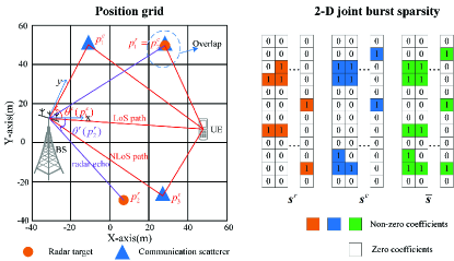
Figure 1: Illustration of location domain radar and communication channels and their non-zero coefficients.

Note that we focus on a 2-D scenario in this paper that is suitable for some application scenarios, such as high-way vehicle networks, in which the mobile user, targets, and communication scatterers are mainly located on the road. However, our proposed scheme can also be easily extended to three-dimensional (3-D) scenarios by adding the third dimension (the z coordinate axis) to the location domain. Besides, the effect of clutters can be incorporated in the proposed model and algorithm. Specifically, the weak clutters can be absorbed into the noise, while the strong clutters can be treated as targets of non-interest, whose parameters will also be estimated. After all the targets have been detected, we can further identify the targets of interest or non-interest based on the properties/features of their parameters.

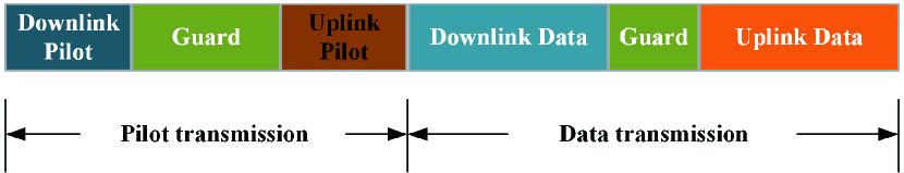
Figure 2: Frame structure of the ISAC system.

The time is divided into frames, with each frame containing two phases: the pilot transmission phase and the data transmission phase, as illustrated in Fig. 2. We will focus on the pilot transmission phase which combines the scattering environment sensing and channel estimation into a single procedure. Specifically, the BS first periodically scans broad angular sectors and transmits downlink pilots to sense the targets at each angular sector. Then the user transmits uplink pilots to the BS for channel estimation. If the user is in a certain angular sector, there will be much overlap between the targets in this angular sector and scatterers associated with this user. Finally, for each angular sector, the BS performs joint scattering environment sensing and channel estimation based on the reflected downlink pilot signal toward this angular sector and the uplink pilot signal of the user in this angular sector. A guard interval is required between downlink and uplink pilots to avoid interference. In the rest of the paper, we shall focus on the problem of joint scattering environment sensing and channel estimation for one angular sector.

II-B Reflected Downlink Pilot Signal

Target sensing aims at detecting the presence of the target and estimating the target location. To achieve this, on the $n\textrm{-th}$ subcarrier for $n\in\mathcal{N}_{b}$, the BS transmits a downlink pilot $\boldsymbol{v}_{n}^{r}\in\mathbb{C}^{M\times 1}$ toward the desired angular sector, and the received signal reflected from the targets can be expressed as

$$\boldsymbol{y}_{n}^{r}=\mathbf{H}_{n}^{r}\boldsymbol{v}_{n}^{r}+\boldsymbol{z}_{n}^{r},\text{ }\forall n\in\mathcal{N}_{b},$$ (1)

where $\mathbf{H}_{n}^{r}\in\mathbb{C}^{M\times M}$ denotes the radar channel matrix, $\boldsymbol{z}_{n}^{r}\in\mathbb{C}^{M\times 1}$ is the additive white Gaussian noise (AWGN) with variance $1/\gamma^{r}$, and $\mathcal{N}_{b}$ is the set of subcarriers used for target sensing in the desired angular sector. Let $\theta^{r}\left(\boldsymbol{p}_{k}^{r}\right)$ and $\tau^{r}\left(\boldsymbol{p}_{k}^{r}\right)$ represent the AoA and delay of the $k\textrm{-th}$ target, respectively, which are related to the position of the BS and the $k\textrm{-th}$ target through

$$\theta^{r}\left(\boldsymbol{p}_{k}^{r}\right) =\arctan\left(\frac{p_{k}^{r,y}-\tilde{p}^{y}}{p_{k}^{r,x}-\tilde{p}^{x}}\right)+\pi\cdotp\mathds{1}\left(p_{k}^{r,x}<\tilde{p}^{x}\right),$$ (2)

$$\tau^{r}\left(\boldsymbol{p}_{k}^{r}\right) =2\left\|\boldsymbol{p}_{b}-\boldsymbol{p}_{k}^{r}\right\|/c,$$

where the angle is calculated anticlockwise with respect to the x-axis, $\mathds{1}\left(\textrm{E}\right)=1$ if the logical expression E is true, and $c$ denotes the speed of light. Then the radar channel matrix can be modeled as

$$\mathbf{H}_{n}^{r}=\sum_{k=0}^{K}x_{k}^{r}e^{-j2\pi nf_{0}\left(\tau^{r}\left(\boldsymbol{p}_{k}^{r}\right)\right)}\boldsymbol{a}\left(\theta^{r}\left(\boldsymbol{p}_{k}^{r}\right)\right)\boldsymbol{a}^{T}\left(\theta^{r}\left(\boldsymbol{p}_{k}^{r}\right)\right),$$ (3)

where $x_{k}^{r}$ represents radar cross section of the $k\textrm{-th}$ target, $f_{0}$ is the subcarrier interval, and $\boldsymbol{a}\left(\theta\right)\in\mathbb{C}^{M\times 1}$ denotes the array response vector at the BS. For the special case of a uniform linear array (ULA), we have

$$\boldsymbol{a}\left(\theta\right)=\frac{1}{\sqrt{M}}\left[1,e^{j\pi\sin\theta},\ldots,e^{j\left(M-1\right)\pi\sin\theta}\right]^{T}.$$ (4)

Note that in (3), we treat the mobile user as the $0\textrm{-th}$ target with its position $\boldsymbol{p}_{0}^{r}\triangleq\boldsymbol{p}_{u}$. If the BS can “see” the user through the radar echo signal, we have $\left|x_{0}^{r}\right|>0$. In this case, the echo signal also directly provides some additional information to assist in locating the user’s position. Otherwise, we have $x_{0}^{r}=0$.

II-C Received Uplink Pilot Signal

The uplink pilot is used to estimate the communication channel as well as sense the communication scatterers between the user and the BS. On the $n\textrm{-th}$ subcarrier for $n\in\mathcal{N}_{u}$, the user transmits an uplink pilot $u_{n}^{c}\in\mathbb{C}$ and then the BS receives the signal, which can be expressed as

$$\boldsymbol{y}_{n}^{c}=\boldsymbol{h}_{n}^{c}u_{n}^{c}+\boldsymbol{z}_{n}^{c},\text{ }\forall n\in\mathcal{N}_{u}$$ (5)

where $\boldsymbol{h}_{n}^{c}\in\mathbb{C}^{M\times 1}$ denotes the communication channel vector, $\boldsymbol{z}_{n}^{c}\in\mathbb{C}^{M\times 1}$ is the the AWGN with variance $1/\gamma^{c}$, and $\mathcal{N}_{u}$ is the set of subcarriers used for uplink channel estimation for the user.

Assume that there is one LoS path, $L$ single-bounce non-LoS (NLoS) paths corresponding to the $L$ communication scatterers, and $J$ multiple-bounce NLoS paths for the communication channel [20]. Let $\theta^{c}\left(\boldsymbol{p}_{u}\right)$ and $\theta^{c}\left(\boldsymbol{p}_{l}^{c}\right)$ represent the AoAs of the LoS path and the $l\textrm{-th}$ single-bounce NLoS path, respectively, which are related to the position of the BS, the user, and the $l\textrm{-th}$ communication scatterer through

$$\theta^{c}\left(\boldsymbol{p}_{u}\right) =\arctan\left(\frac{p^{y}-\tilde{p}^{y}}{p^{x}-\tilde{p}^{x}}\right)+\pi\cdotp\mathds{1}\left(p^{x}<\tilde{p}^{x}\right),$$ (6)

$$\theta^{c}\left(\boldsymbol{p}_{l}^{c}\right) =\arctan\left(\frac{p_{l}^{c,y}-\tilde{p}^{y}}{p_{l}^{c,x}-\tilde{p}^{x}}\right)+\pi\cdotp\mathds{1}\left(p_{l}^{c,x}<\tilde{p}^{x}\right).$$

Clearly, the relative delay of the $l\textrm{-th}$ single-bounce NLoS path (relative to the LoS path) can be expressed as

$$\tau^{c}\left(\boldsymbol{p}_{l}^{c},\boldsymbol{p}_{u}\right)=\left(\left\|\boldsymbol{p}_{b}-\boldsymbol{p}_{l}^{c}\right\|+\left\|\boldsymbol{p}_{u}-\boldsymbol{p}_{l}^{c}\right\|-\left\|\boldsymbol{p}_{b}-\boldsymbol{p}_{u}\right\|\right)/c.$$ (7)

Furthermore, let $\tilde{\theta}_{j}^{c}$ and $\tilde{\tau}_{j}^{c}$ denote the AoA and relative delay of the $j\textrm{-th}$ multiple-bounce NLoS path, respectively.

Then the communication channel vector can be modeled as

$$\boldsymbol{h}_{n}^{c}=\boldsymbol{h}_{n}^{c,\textrm{L}}+\boldsymbol{h}_{n}^{c,\textrm{SL}}+\boldsymbol{h}_{n}^{c,\textrm{ML}},$$ (8)

with

$$\boldsymbol{h}_{n}^{c,\textrm{L}} =x_{0}^{c}e^{-j2\pi nf_{0}\tau_{o}}\boldsymbol{a}\left(\theta^{c}\left(\boldsymbol{p}_{u}\right)\right),$$ (9a)

$$\boldsymbol{h}_{n}^{c,\textrm{SL}} =\sum_{l=1}^{L}x_{l}^{c}e^{-j2\pi nf_{0}\left(\tau^{c}\left(\boldsymbol{p}_{l}^{c},\boldsymbol{p}_{u}\right)+\tau_{o}\right)}\boldsymbol{a}\left(\theta^{c}\left(\boldsymbol{p}_{l}^{c}\right)\right),$$ (9b)

$$\boldsymbol{h}_{n}^{c,\textrm{ML}} =\sum_{j=1}^{J}\tilde{x}_{j}^{c}e^{-j2\pi nf_{0}\left(\tilde{\tau}_{j}^{c}+\tau_{o}\right)}\boldsymbol{a}\left(\tilde{\theta}_{j}^{c}\right),$$ (9c)

where $\boldsymbol{h}_{n}^{c,\textrm{L}}$, $\boldsymbol{h}_{n}^{c,\textrm{SL}}$, and $\boldsymbol{h}_{n}^{c,\textrm{ML}}$ represent the channel response vectors of the LoS path, single-bounce NLoS paths, and multiple-bounce NLoS paths, respectively, $x_{0}^{c}$, $x_{l}^{c}$, and $\tilde{x}_{j}^{c}$ denote the channel gains of the LoS path, the $l\textrm{-th}$ single-bounce NLoS path, and the $j\textrm{-th}$ multiple-bounce NLoS path, respectively, and $\tau_{o}$ is the time offset (relative to the LoS path) caused by the timing synchronization error at the BS.

III Sparse Bayesian Inference Formulation

In this section, we first obtain a sparse representation of the radar and communication channels. Then, we introduce a three-layer sparse prior and a spatially non-stationary MRF model to capture the 2-D joint burst sparsity of the location domain channels. Finally, we formulate the problem of joint scattering environment sensing and channel estimation as a sparse Bayesian inference problem.

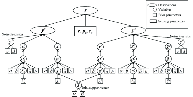
Figure 3: Illustration of the three-layer sparse prior model.

III-A Location Domain Sparse Representation of Channels

We introduce a grid-based solution to obtain a sparse representation of the channels for better sensing and estimation performance. Specifically, we first define a 2-D uniform grid $\left\{\overline{\boldsymbol{r}}_{1},\ldots,\overline{\boldsymbol{r}}_{Q}\right\}\subset\mathcal{R}$ with size $H\times W$ of $Q\gg K+L$ positions for localizing the radar targets and communication scatterers, as illustrated in Fig. 1, where the position grid points are in a square area with $H$ rows and $W$ columns. Then, we define a fixed grid $\left\{\overline{\theta}_{1},...,\overline{\theta}_{U}\right\}$ of $U$ AoA points and a uniform grid $\left\{\overline{\tau}_{1},...,\overline{\tau}_{V}\right\}\subset\left[\tau_{min},\tau_{max}\right]$ of $V$ time-of-arrival (ToA) points to estimate the multiple-bounce NLoS channel vector, where $\left\{\sin\overline{\theta}_{u}\right\}_{u=1}^{U}$ are uniformly distributed in the range $\left[-1,1\right]$ and the delay plus time offsets of multiple-bounce NLoS paths, $\tilde{\tau}_{j}^{c}+\tau_{o},\forall j$, are assumed to be within the range $\left[\tau_{min},\tau_{max}\right]$.

In practice, the true positions/AoAs/ToAs usually do not lie exactly on the $Q$/$U$/$V$ discrete position/angle/delay grid points. In this case, there will be an energy leakage effect, and thus we cannot obtain an exact sparse representation of the corresponding channels. The total energy of multiple-bounce NLoS paths is usually small compared to the total energy of LoS and single-bounce NLoS paths. Therefore, the energy leakage effect caused by the AoA and ToA mismatches is negligible compared to the noise power. However, it is essential to overcome the position mismatches for high-resolution localization. One common solution is to introduce a dynamic position grid, denoted by $\boldsymbol{r}\triangleq\left[\boldsymbol{r}_{1};\ldots;\boldsymbol{r}_{Q}\right]$, instead of only using a fixed position grid. In this case, there always exists an $\boldsymbol{r}^{*}$ that covers the true position of all targets and communication scatterers. In general, the uniform grid is chosen as the initial point for $\boldsymbol{r}$ in the algorithm, which makes it easier to find a good solution for the non-convex MAP estimation problem [9].

Then we define the sparse basis with a dynamic position grid for the radar channel matrix and the single-bounce NLoS communication channel vector as

$$\mathbf{A}\left(\boldsymbol{r}\right)\triangleq\left[\boldsymbol{a}\left(\theta^{r}\left(\boldsymbol{r}_{1}\right)\right),\ldots,\boldsymbol{a}\left(\theta^{r}\left(\boldsymbol{r}_{Q}\right)\right)\right]\in\mathbb{C}^{M\times Q}.$$ (10)

Based on the angular and delay domain grids, we define the on-grid basis for the multiple-bounce NLoS communication channel vector as

$$\overline{\mathbf{A}} \triangleq\left[\boldsymbol{a}\left(\overline{\theta}_{1}\right),\ldots,\boldsymbol{a}\left(\overline{\theta}_{U}\right)\right]\in\mathbb{C}^{M\times U},$$ (11)

$$\overline{\mathbf{D}} \triangleq\left[\boldsymbol{d}\left(\overline{\tau}_{1}\right),\ldots,\boldsymbol{d}\left(\overline{\tau}_{V}\right)\right]\in\mathbb{C}^{\left|\mathcal{N}_{u}\right|\times V},$$

where $\boldsymbol{d}\left(\tau\right)\triangleq\left[e^{-j2\pi nf_{0}\tau}\right]_{n\in\mathcal{N}_{u}}\in\mathbb{C}^{\left|\mathcal{N}_{u}\right|\times 1}$ denotes the delay domain basis vector.

The sparse representation of the radar channel matrix and the single-bounce NLoS communication channel vector on the $n\textrm{-th}$ subcarrier corresponding to (3) and (9b) are respectively given by

$$\mathbf{H}_{n}^{r} =\mathbf{A}\left(\boldsymbol{r}\right)\mathbf{D}_{n}^{r}\textrm{diag}\left(\boldsymbol{x}^{r}\right)\mathbf{A}^{T}\left(\boldsymbol{r}\right)$$

$$+x_{0}^{r}e^{-j2\pi nf_{0}\left(\tau^{r}\left(\boldsymbol{p}_{u}\right)\right)}\boldsymbol{a}\left(\theta^{r}\left(\boldsymbol{p}_{u}\right)\right)\boldsymbol{a}^{T}\left(\theta^{r}\left(\boldsymbol{p}_{u}\right)\right),$$ (12)

$$\boldsymbol{h}_{n}^{c,\textrm{SL}} =\mathbf{A}\left(\boldsymbol{r}\right)\mathbf{D}_{n}^{c}\boldsymbol{x}^{c},$$ (13)

where $\mathbf{D}_{n}^{r}$ and $\mathbf{D}_{n}^{c}$ are diagonal matrices with the $q\textrm{-th}$ diagonal elements being $e^{-j2\pi nf_{0}\tau^{r}\left(\boldsymbol{r}_{q}\right)}$ and $e^{-j2\pi nf_{0}\left(\tau^{c}\left(\boldsymbol{r}_{q},\boldsymbol{p}_{u}\right)+\tau_{o}\right)}$, respectively, $\boldsymbol{x}^{r}\in\mathbb{C}^{Q\times 1}$ and $\boldsymbol{x}^{c}\in\mathbb{C}^{Q\times 1}$ are called the location domain sparse radar channel vector and single-bounce NLoS communication channel vector. $\boldsymbol{x}^{r}$ and $\boldsymbol{x}^{c}$ only have a few non-zero elements corresponding to the position of targets and communication scatterers, respectively. Specifically, the $q\textrm{-th}$ element of $\boldsymbol{x}^{r}$, denoted by $x_{q}^{r}$, represents the complex reflection coefficient of a target lying in the position $\boldsymbol{r}_{q}$. The $q\textrm{-th}$ element of $\boldsymbol{x}^{c}$, denoted by $x_{q}^{c}$, represents the complex channel gain of the channel path with the corresponding communication scatterer lying in the position $\boldsymbol{r}_{q}$.

Using the on-gird basis $\overline{\mathbf{A}}$ and $\overline{\mathbf{D}}$, the multiple-bounce NLoS communication channel vectors on all subcarriers can be expressed as

$$\left[\boldsymbol{h}_{n}^{c,\textrm{ML}}\right]_{n\in\mathcal{N}_{u}}= \textrm{vec}\left(\overline{\mathbf{A}}\widetilde{\mathbf{X}}^{c}\overline{\mathbf{D}}^{T}\right)=\left(\overline{\mathbf{D}}\otimes\overline{\mathbf{A}}\right)\widetilde{\boldsymbol{x}}^{c},$$ (14)

where $\widetilde{\mathbf{X}}^{c}\in\mathbb{C}^{U\times V}$ is the delay-angular domain sparse multiple-bounce NLoS communication channel matrix, and $\widetilde{\boldsymbol{x}}^{c}\triangleq\textrm{vec}\left(\widetilde{\mathbf{X}}^{c}\right)\in\mathbb{C}^{UV\times 1}$.

III-B Markov Random Field for 2-D Joint Burst Sparsity

We shall introduce a three-layer sparse prior model, where a Markov random field model is used to capture the 2-D joint burst sparsity of the location domain channels. Specifically, let $\boldsymbol{\rho}^{r}\triangleq\left[\rho_{1}^{r},\ldots,\rho_{Q}^{r}\right]^{T}$ and $\boldsymbol{\rho}^{c}\triangleq\left[\rho_{1}^{c},\ldots,\rho_{Q}^{c}\right]^{T}$ represent the precision vectors of $\boldsymbol{x}^{r}$ and $\boldsymbol{x}^{c}$, respectively, where $1/\rho_{q}^{r}$ and $1/\rho_{q}^{c}$ are the variance of $x_{q}^{r}$ and $x_{q}^{c}$, respectively. Let $\boldsymbol{s}^{r}\triangleq\left[s_{1}^{r},\ldots,s_{Q}^{r}\right]^{T}\in\left\{-1,1\right\}^{Q}$ and $\boldsymbol{s}^{c}\triangleq\left[s_{1}^{c},\ldots,s_{Q}^{c}\right]^{T}\in\left\{-1,1\right\}^{Q}$ represent the support vectors of $\boldsymbol{x}^{r}$ and $\boldsymbol{x}^{c}$, respectively. If there is a radar target (communication scatterer) around the $q\textrm{-th}$ position grid $\boldsymbol{r}_{q}$, we have $s_{q}^{r}=1$ and $x_{q}^{r}$ is non-zero ($s_{q}^{c}=1$ and $x_{q}^{c}$ is non-zero). Otherwise, we have $s_{q}^{r}=-1$ and $x_{q}^{r}=0$ ($s_{q}^{c}=-1$ and $x_{q}^{c}=0$). Then, we introduce a joint support vector $\overline{\boldsymbol{s}}\triangleq\left[\overline{s}_{1},\ldots,\overline{s}_{Q}\right]^{T}\in\left\{-1,1\right\}^{Q}$ to represent the union of the positions of the radar targets and communication scatterers. If either $s_{q}^{r}=1$ or $s_{q}^{c}=1$, we have $\overline{s}_{q}=1$. Otherwise, we have $\overline{s}_{q}=-1$. The joint distribution of $\boldsymbol{x}^{r}$, $\boldsymbol{x}^{c}$, $\boldsymbol{\rho}^{r}$, $\boldsymbol{\rho}^{c}$, $\boldsymbol{s}^{r}$, $\boldsymbol{s}^{c}$, and $\overline{\boldsymbol{s}}$ is represented as

$$p\left(\boldsymbol{x}^{r},\boldsymbol{x}^{c},\boldsymbol{\rho}^{r},\boldsymbol{\rho}^{c},\boldsymbol{s}^{r},\boldsymbol{s}^{c},\overline{\boldsymbol{s}}\right)$$ (15)

$$= \underbrace{p\left(\boldsymbol{s}^{r},\boldsymbol{s}^{c},\overline{\boldsymbol{s}}\right)}_{\textrm{Support}}\underbrace{p\left(\boldsymbol{\rho}^{r}\mid\boldsymbol{s}^{r}\right)p\left(\boldsymbol{\rho}^{c}\mid\boldsymbol{s}^{c}\right)}_{\textrm{Precision}}\underbrace{p\left(\boldsymbol{x}^{r}\mid\boldsymbol{\rho}^{r}\right)p\left(\boldsymbol{x}^{c}\mid\boldsymbol{\rho}^{c}\right)}_{\textrm{Sparse\ signal}}.$$

The three-layer sparse prior model is shown in Fig. 3. A similar three-layer model has been considered in [16, 18] and is shown to be more flexible to capture the structured sparsity of realistic channels.

The sparse signals $\boldsymbol{x}^{r}$ and $\boldsymbol{x}^{c}$ follow complex Gaussian distributions with zero mean and variance $1/\boldsymbol{\rho}^{r}$ and $1/\boldsymbol{\rho}^{c}$, respectively. Moreover, conditioned on $\boldsymbol{\rho}^{r}$ and $\boldsymbol{\rho}^{c}$, the elements of $\boldsymbol{x}^{r}$ and $\boldsymbol{x}^{c}$ are assumed to be independent, i.e.,

$$p\left(\boldsymbol{x}^{r}\mid\boldsymbol{\rho}^{r}\right) =\prod_{q}p\left(x_{q}^{r}\mid\rho_{q}^{r}\right)=\prod_{q}\mathcal{CN}\left(x_{q}^{r};0,1/\rho_{q}^{r}\right),$$ (16)

$$p\left(\boldsymbol{x}^{c}\mid\boldsymbol{\rho}^{c}\right) =\prod_{q}p\left(x_{q}^{c}\mid\rho_{q}^{c}\right)=\prod_{q}\mathcal{CN}\left(x_{q}^{c};0,1/\rho_{q}^{c}\right).$$

The conditional distributions $p\left(\boldsymbol{\rho}^{r}\mid\boldsymbol{s}^{r}\right)$ and $p\left(\boldsymbol{\rho}^{c}\mid\boldsymbol{s}^{c}\right)$ are respectively given by

$$p\left(\boldsymbol{\rho}^{r}\mid\boldsymbol{s}^{r}\right)= \prod_{q}\left(\delta\left(s_{q}^{r}-1\right)\textrm{Gamma}\left(\rho_{q}^{r};a,b\right)\right.$$ (17)

$$+ \left.\delta\left(s_{q}^{r}+1\right)\textrm{Gamma}\left(\rho_{q}^{r};\overline{a},\overline{b}\right)\right),$$

$$p\left(\boldsymbol{\rho}^{c}\mid\boldsymbol{s}^{c}\right)= \prod_{q}\left(\delta\left(s_{q}^{c}-1\right)\textrm{Gamma}\left(\rho_{q}^{c};a,b\right)\right.$$

$$+ \left.\delta\left(s_{q}^{c}+1\right)\textrm{Gamma}\left(\rho_{q}^{c};\overline{a},\overline{b}\right)\right),$$

where $\delta\left(\cdot\right)$ is the Dirac Delta function. When $s_{q}^{r}=1$, $x_{q}^{r}$ is a non-zero element and the corresponding variance $1/\rho_{q}^{r}$ is $\Theta\left(1\right)$. In this case, $a$ and $b$ should be chosen to satisfy $\tfrac{a}{b}=\mathbb{E}\left(\rho_{q}^{r}\right)=\Theta\left(1\right)$. When $s_{q}^{r}=-1$, $x_{q}^{r}$ is a zero element and the corresponding variance $1/\rho_{q}^{r}$ is close to zero. In this case, $\overline{a}$ and $\overline{b}$ should be chosen to satisfy $\tfrac{\overline{a}}{\overline{b}}=\mathbb{E}\left(\rho_{q}^{r}\right)\gg 1$. A typical value is $a=1$, $b=1$, $\overline{a}=1$, and $\overline{b}=10^{-5}$ [18]. Since the gamma prior is conjugate to the Gaussian prior, we can derive the close-form expressions when performing Bayesian inference. The details will be elaborated in Section IV.

The joint distribution of support vectors can be further decomposed into

$$p\left(\boldsymbol{s}^{r},\boldsymbol{s}^{c},\overline{\boldsymbol{s}}\right) =p\left(\boldsymbol{s}^{r}\mid\overline{\boldsymbol{s}}\right)p\left(\boldsymbol{s}^{c}\mid\overline{\boldsymbol{s}}\right)p\left(\overline{\boldsymbol{s}}\right)$$ (18)

$$=\prod_{q}p\left(s_{q}^{r}\mid\overline{s}_{q}\right)\prod_{q}p\left(s_{q}^{c}\mid\overline{s}_{q}\right)p\left(\overline{\boldsymbol{s}}\right),$$

where the conditional distributions are given by

$$p\left(s_{q}^{r}\mid\overline{s}_{q}\right) =\delta\left(\overline{s}_{q}+1\right)\delta\left(s_{q}^{r}+1\right)$$ (19)

$$+\delta\left(\overline{s}_{q}-1\right)\left(\delta\left(s_{q}^{r}-1\right)\lambda{}_{q}^{r}+\delta\left(s_{q}^{r}+1\right)\left(1-\lambda{}_{q}^{r}\right)\right),$$

$$p\left(s_{q}^{c}\mid\overline{s}_{q}\right) =\delta\left(\overline{s}_{q}+1\right)\delta\left(s_{q}^{c}+1\right)$$

$$+\delta\left(\overline{s}_{q}-1\right)\left(\delta\left(s_{q}^{c}-1\right)\lambda_{q}^{c}+\delta(s_{q}^{c}+1)\left(1-\lambda_{q}^{c}\right)\right),$$

where $\lambda{}_{q}^{r}$ and $\lambda_{q}^{c}$ represent the probability of $s_{q}^{r}=1$ and $s_{q}^{c}=1$ conditioned on $\overline{s}_{q}=1$, respectively.

Moreover, we use a spatially non-stationary Markov random field model to describe the 2-D joint burst sparsity of $\boldsymbol{x}^{r}$ and $\boldsymbol{x}^{c}$. Based on the Ising model [22, 23], the joint support vector can be modeled as

$$p\left(\overline{\boldsymbol{s}}\right) =\frac{1}{Z\left(\boldsymbol{\zeta}\right)}\exp\left(\sum_{q=1}^{Q}\left(\frac{1}{2}\sum_{i\in\mathcal{N}_{q}}\beta_{iq}\overline{s}_{i}-\alpha_{q}\right)\overline{s}_{q}\right)$$ (20)

$$=\frac{1}{Z\left(\boldsymbol{\zeta}\right)}\left(\stackrel{{\scriptstyle[}}{{q}}=1]{Q}{\prod}\underset{i\in\mathcal{N}_{q}}{\prod}\varphi\left(\overline{s}_{q},\overline{s}_{i}\right)\right)^{\frac{1}{2}}\prod_{q=1}^{Q}\psi\left(\overline{s}_{q}\right),$$

where $\varphi\left(\overline{s}_{q},\overline{s}_{i}\right)=\exp\left(\beta_{iq}\overline{s}_{i}\overline{s}_{q}\right)$, $\psi\left(\overline{s}_{q}\right)=\exp\left(-\alpha_{q}\overline{s}_{q}\right)$, $\mathcal{N}_{q}$ denotes the index set for the neighbors of $\overline{s}_{q}$, $\boldsymbol{\zeta}\triangleq\left\{\alpha_{q},\beta_{iq}\mid i\in\mathcal{N}_{q},\forall q\right\}$ denotes the MRF parameters, and $Z\left(\boldsymbol{\zeta}\right)$ denotes the partition function. Since $\alpha_{q}$ and $\beta_{iq}$ depends on the position index $q$, the MRF in (20) is spatially non-stationary, which helps to model scattering clusters with diverse random sizes and positions. Specifically, a higher value of $\beta_{iq}$ implies a larger size for non-zero bursts, and a higher value of $\alpha_{q}$ implies sparser signal activity.

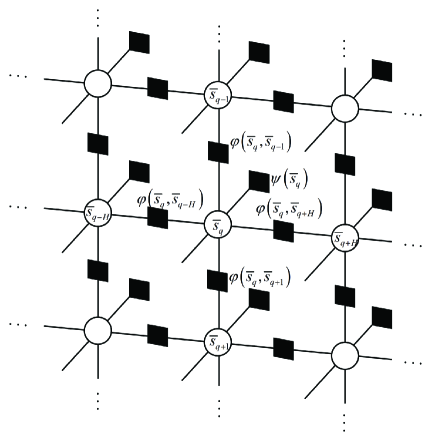
Figure 4: Factor graph of the 4-connected MRF model.

We try to recover the joint support vector $\overline{\boldsymbol{s}}$ associated with the 2-D position grid of $Q=H\times W$ points. In this case, the 4-connected MRF model is suitable to process such a 2-D sparse signal recovery problem. The factor graph of the 4-connected MRF model is shown in Fig. 4. In the MRF model, the variable nodes $\left\{\overline{s}_{q}\right\}_{q=1}^{Q}$ are scheduled in $H$ rows and $W$ columns. Most of the variable nodes have four neighboring nodes, except for the nodes at the boundaries. To be specific, the left, right, top, and bottom neighboring nodes of $\overline{s}_{q}$ are $\overline{s}_{q-H}$, $\overline{s}_{q+H}$, $\overline{s}_{q-1}$, and $\overline{s}_{q+1}$, respectively. Two types of factor nodes are involved in the factor graph. The factor node $\varphi\left(\overline{s}_{q},\overline{s}_{i}\right)$ connecting $\overline{s}_{q}$ and $\overline{s}_{i}$ describes the correlation between two neighboring nodes, while the factor node $\psi\left(\overline{s}_{q}\right)$ connected to $\overline{s}_{q}$ directly affects the sparse probability of $\overline{s}_{q}$.

To automatically learn the noise precision, we assume a gamma distribution with shape parameter $c$ and rate parameter $d$ as the prior for $\gamma^{r}$ and $\gamma^{c}$, i.e.,

$$p\left(\gamma^{r}\right) =\textrm{Gamma}\left(\gamma^{r};c,d\right),$$ (21)

$$p\left(\gamma^{c}\right) =\textrm{Gamma}\left(\gamma^{c};c,d\right).$$

The sparse prior model for $x_{0}^{r}$, $x_{0}^{c}$, and $\widetilde{\boldsymbol{x}}^{c}$ is similar to that of $\boldsymbol{x}^{r}$ and $\boldsymbol{x}^{c}$ except that there is no joint support vector, as shown in Fig. 3, where $\rho_{0}^{r}$, $\rho_{0}^{c}$, and $\boldsymbol{\widetilde{\rho}}^{c}$ denote the precision of $x_{0}^{r}$, $x_{0}^{c}$, and $\widetilde{\boldsymbol{x}}^{c}$, respectively, $s_{0}^{r},$ $s_{0}^{c}$, and $\widetilde{\boldsymbol{s}}^{c}$ denote the support of $x_{0}^{r}$, $x_{0}^{c}$, and $\widetilde{\boldsymbol{x}}^{c}$, respectively, $\lambda_{0}^{r}$, $\lambda_{0}^{r}$, and $\widetilde{\lambda_{j}}^{c},\forall j$ give the probability of $s_{0}^{r}=1$, $s_{0}^{c}=1$, and $\widetilde{s}_{j}^{c}=1,\forall j$, respectively.

The unknown parameters of the probability model, denoted by $\left\{\lambda{}_{q}^{r},\lambda{}_{q}^{c},\lambda_{0}^{r},\lambda_{0}^{c},\widetilde{\lambda_{j}}^{c},\boldsymbol{\zeta}\right\}$, can be automatically learned based on the EM method. However, the non-stationary MRF in (20) is quite complicated and the corresponding model parameters $\boldsymbol{\zeta}$ cannot be easily learned via the conventional EM method. We will describe how to learn MRF parameters approximately via a low-complexity method in Subsection IV-E.

III-C Sparse Bayesian Inference with Uncertain Parameters

Using the location domain sparse representation in (12) and (13) and the angle-delay domain sparse representation in (14), the reflected downlink pilot signal and received uplink pilot signal on all available subcarriers can be expressed as

$$\boldsymbol{y}^{r} =\boldsymbol{\Phi}^{r}\left(\boldsymbol{r},\boldsymbol{p}_{u}\right)\left[x_{0}^{r},\left(\boldsymbol{x}^{r}\right)^{T}\right]^{T}+\boldsymbol{z}^{r},$$ (22a)

$$\boldsymbol{y}^{c} =\boldsymbol{\Phi}^{c}\left(\boldsymbol{r},\boldsymbol{p}_{u},\tau_{o}\right)\left[x_{0}^{c},\left(\boldsymbol{x}^{c}\right)^{T},\left(\widetilde{\boldsymbol{x}}^{c}\right)^{T}\right]^{T}+\boldsymbol{z}^{c},$$ (22b)

where $\boldsymbol{y}^{r}\triangleq\left[\boldsymbol{y}_{n}^{r}\right]_{n\in\mathcal{N}_{b}}\in\mathbb{C}^{M\left|\mathcal{N}_{b}\right|\times 1}$, $\boldsymbol{y}^{c}\triangleq\left[\boldsymbol{y}_{n}^{c}\right]_{n\in\mathcal{N}_{u}}\in\mathbb{C}^{M\left|\mathcal{N}_{u}\right|\times 1}$, $\boldsymbol{z}^{r}\triangleq\left[\boldsymbol{z}_{n}^{r}\right]_{n\in\mathcal{N}_{b}}\in\mathbb{C}^{M\left|\mathcal{N}_{b}\right|\times 1}$, and $\boldsymbol{z}^{c}\triangleq\left[\boldsymbol{z}_{n}^{c}\right]_{n\in\mathcal{N}_{u}}\in\mathbb{C}^{M\left|\mathcal{N}_{u}\right|\times 1}$.

The radar and communication measurement matrices in (22a) and (22b) can be decomposed into some submatrices, respectively, i.e.,

$$\boldsymbol{\Phi}^{r}\left(\boldsymbol{r},\boldsymbol{p}_{u}\right) \triangleq\left[\boldsymbol{\Phi}^{r,0},\boldsymbol{\Phi}^{r,1}\right]\in\mathbb{C}^{M\left|\mathcal{N}_{b}\right|\times\left(Q+1\right)},$$ (23)

$$\boldsymbol{\Phi}^{c}\left(\boldsymbol{r},\boldsymbol{p}_{u},\tau_{o}\right) \triangleq\left[\boldsymbol{\Phi}^{c,0},\boldsymbol{\Phi}^{c,1},\boldsymbol{\Phi}^{c,2}\right]\in\mathbb{C}^{M\left|\mathcal{N}_{u}\right|\times\left(Q+UV+1\right)},$$

where

$$\boldsymbol{\Phi}^{r,0} =\left[e^{-j2\pi nf_{0}\left(\tau^{r}\left(\boldsymbol{p}_{u}\right)\right)}\boldsymbol{a}\left(\theta^{r}\left(\boldsymbol{p}_{u}\right)\right)\boldsymbol{a}^{T}\left(\theta^{r}\left(\boldsymbol{p}_{u}\right)\right)\boldsymbol{v}_{n}^{r}\right]_{n\in\left|\mathcal{N}_{b}\right|},$$

$$\boldsymbol{\bar{\Phi}}^{r,1} =\left[\left(\left(\boldsymbol{v}_{n}^{r}\right)^{T}\mathbf{A}\left(\boldsymbol{r}\right)\right)\otimes\left(\mathbf{A}\left(\boldsymbol{r}\right)\mathbf{D}_{n}^{r}\right)\right]_{n\in\left|\mathcal{N}_{b}\right|},$$

$$\boldsymbol{\Phi}^{c,0} =\left[u_{n}^{c}e^{-j2\pi nf_{0}\tau_{o}}\boldsymbol{a}\left(\theta^{c}\left(\boldsymbol{p}_{u}\right)\right)\right]_{n\in\left|\mathcal{N}_{u}\right|},$$

$$\boldsymbol{\Phi}^{c,1} =\left[u_{n}^{c}\mathbf{A}\left(\boldsymbol{r}\right)\mathbf{D}_{n}^{c}\right]_{n\in\left|\mathcal{N}_{u}\right|},$$

$$\boldsymbol{\Phi}^{c,2} =\left(\textrm{diag}\left(\left[u_{n}^{c}\right]_{n\in\left|\mathcal{N}_{u}\right|}\right)\mathbf{\overline{D}}\right)\otimes\mathbf{\overline{A}},$$ (24)

where $\boldsymbol{\Phi}^{r,1}\in\mathbb{C}^{M\left|\mathcal{N}_{b}\right|\times Q}$ consists of the $\left(\left(q-1\right)Q+q\right)\textrm{-th}$ column of $\boldsymbol{\bar{\Phi}}^{r,1}$ for $q=1,\ldots,Q$.

For convenience, we combine (22a) and (22b) into a linear observation model as

$$\boldsymbol{y}=\boldsymbol{\Phi}\left(\boldsymbol{\vartheta}\right)\boldsymbol{x}+\boldsymbol{z},$$ (25)

where $\boldsymbol{\xi}\triangleq\left\{\boldsymbol{r},\boldsymbol{p}_{u},\tau_{o}\right\}$ is the collection of sensing parameters, $\boldsymbol{y}\triangleq\left[\left(\boldsymbol{y}^{r}\right)^{T},\left(\boldsymbol{y}^{c}\right)^{T}\right]^{T}$, $\boldsymbol{z}\triangleq\left[\left(\boldsymbol{z}^{r}\right)^{T},\left(\boldsymbol{z}^{c}\right)^{T}\right]^{T}$, $\boldsymbol{x}\triangleq\left[x_{0}^{r},\left(\boldsymbol{x}^{r}\right)^{T},x_{0}^{c},\left(\boldsymbol{x}^{c}\right)^{T},\left(\widetilde{\boldsymbol{x}}^{c}\right)^{T}\right]^{T}$, and $\boldsymbol{\Phi}\left(\boldsymbol{\vartheta}\right)\triangleq\mathrm{\textrm{BlockDiag}}\left(\boldsymbol{\Phi}^{r}\left(\boldsymbol{\vartheta}\right),\boldsymbol{\Phi}^{c}\left(\boldsymbol{\vartheta}\right)\right)$.

To simply the notation, the precision vector and the support vector of $\boldsymbol{x}$ are respectively defined as

$$\boldsymbol{\rho} \triangleq\left[\rho_{0}^{r},\left(\boldsymbol{\rho}^{r}\right)^{T},\rho_{0}^{c},\left(\boldsymbol{\rho}^{c}\right)^{T},\left(\widetilde{\boldsymbol{\rho}}^{c}\right)^{T}\right]^{T},$$

$$\boldsymbol{s} \triangleq\left[s_{0}^{r},\left(\boldsymbol{s}^{r}\right)^{T},s_{0}^{c},\left(\boldsymbol{s}^{c}\right)^{T},\left(\widetilde{\boldsymbol{s}}^{c}\right)^{T}\right]^{T}.$$

Our primary goal is to estimate the channel vector $\boldsymbol{x}$, the support vector $\boldsymbol{s}$, and the uncertain parameters $\boldsymbol{\xi}\triangleq\left\{\boldsymbol{\vartheta},\boldsymbol{\zeta}\right\}$ given observation $\boldsymbol{y}$ in model (25). To be specific, for given $\boldsymbol{\xi}$, we aim at computing the conditional marginal posteriors, i.e., $p\left(\boldsymbol{x}\mid\boldsymbol{y};\boldsymbol{\xi}\right)$ and $p\left(s_{i}\mid\boldsymbol{y};\boldsymbol{\xi}\right),\forall i$. On the other hand, the uncertain parameters $\boldsymbol{\xi}$ are obtained by the MAP estimator as follows:

$$\boldsymbol{\xi}^{\ast} =\underset{\boldsymbol{\xi}}{\arg\max}\ln p\left(\boldsymbol{\xi}\mid\boldsymbol{y}\right)$$ (26)

$$=\underset{\boldsymbol{\xi}}{\arg\max}\sum_{\overline{\boldsymbol{s}}}\ln\int_{\boldsymbol{v}}p\left(\boldsymbol{y},\boldsymbol{v},\overline{\boldsymbol{s}};\boldsymbol{\xi}\right)p\left(\boldsymbol{\vartheta}\right),$$

where $\boldsymbol{v}\triangleq\left\{\boldsymbol{x},\boldsymbol{\rho},\boldsymbol{s},\gamma^{r},\gamma^{c}\right\}$ and $p\left(\boldsymbol{\vartheta}\right)$ denotes the known prior distribution of $\boldsymbol{\vartheta}$. Once we obtain the MAP estimate of $\boldsymbol{\xi}^{\ast}$, we can obtain the minimum mean square error (MMSE) estimate of $\boldsymbol{x}$ as $\boldsymbol{x}^{*}=\int_{\boldsymbol{x}}\boldsymbol{x}p\left(\boldsymbol{x}\mid\boldsymbol{y};\boldsymbol{\xi}^{\ast}\right)$ and the MAP estimate of $\boldsymbol{s}$ as $s_{i}^{\ast}=\arg\max_{s_{i}}p\left(s_{i}\mid\boldsymbol{y};\boldsymbol{\xi}^{\ast}\right),\forall i$.

However, the corresponding factor graph of the probability model contains loops and the associated sparse Bayesian inference problem is NP-hard. Therefore, it is exceedingly challenging to calculate the above conditional marginal posteriors precisely. In the following section, we present the Turbo-IF-VBI algorithm, which uses the turbo approach to calculate approximate marginal posteriors and applies a variation of the EM method to find an approximate solution for (26).

IV Turbo-IF-VBI Algorithm

IV-A Outline of the Turbo-IF-VBI Algorithm

The primary goal of the Turbo-IF-VBI algorithm is to simultaneously maximize the marginal log-posterior $\ln p\left(\boldsymbol{y},\boldsymbol{\xi}\right)$ with respect to the uncertain parameters $\boldsymbol{\xi}$ in (26) and approximately calculate the conditional posteriors. As illustrated in Fig. 5, the Turbo-IF-VBI algorithm iterates between the next two major steps until convergence.

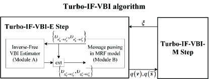
Figure 5: Framework of the Turbo-IF-VBI algorithm.

• Turbo-IF-VBI-E Step: For given $\boldsymbol{\xi}^{\left(t\right)}$ in the $t\textrm{-th}$ iteration, calculate the approximate marginal posteriors, denoted by $q\left(\boldsymbol{v}\mid\boldsymbol{y};\boldsymbol{\xi}^{\left(t\right)}\right)$ and $q\left(\overline{\boldsymbol{s}}\mid\boldsymbol{y};\boldsymbol{\xi}^{\left(t\right)}\right)$, based on the turbo approach.

• Turbo-IF-VBI-M Step: Construct a surrogate function for $\ln p\left(\boldsymbol{y},\boldsymbol{\xi}\right)$ based on $q\left(\boldsymbol{v}\mid\boldsymbol{y};\boldsymbol{\xi}^{\left(t\right)}\right)$ and $q\left(\overline{\boldsymbol{s}}\mid\boldsymbol{y};\boldsymbol{\xi}^{\left(t\right)}\right)$ obtained in the Turbo-IF-VBI-E Step, then maximize the surrogate function with respect to $\boldsymbol{\xi}$.

The Turbo-IF-VBI-E Step is an inverse-free algorithm by combining the IF-VBI estimator and message passing via the turbo framework, where the IF-VBI avoids the matrix inverse operation via maximizing a relaxed ELBO. Furthermore, the Turbo-IF-VBI-M Step is challenging as the surrogate function constructed by the conventional EM method involves exponential computational complexity. To overcome this challenge, we propose a low-complexity method based on pseudo-likelihood approximation to learn MRF parameters. In the following, we first elaborate on how to approximately calculate $q\left(\boldsymbol{v}\mid\boldsymbol{y};\boldsymbol{\xi}^{\left(t\right)}\right)$ and $q\left(\overline{\boldsymbol{s}}\mid\boldsymbol{y};\boldsymbol{\xi}^{\left(t\right)}\right)$ in the Turbo-IF-VBI-E Step. Then, we show how to update $\boldsymbol{\xi}$ in the Turbo-IF-VBI-M Step.

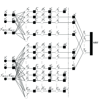
Figure 6: Factor graph of the joint distribution $p\left(\boldsymbol{y},\boldsymbol{v},\overline{\boldsymbol{s}};\boldsymbol{\xi}\right)$.

TABLE I: Factors, Distributions and Functional forms in Fig. 6. $\boldsymbol{\Phi}_{m}^{r}\left(\boldsymbol{\vartheta}\right)$ and $\boldsymbol{\Phi}_{m}^{c}\left(\boldsymbol{\vartheta}\right)$ denote the $m\textrm{-th}$ row of $\boldsymbol{\Phi}^{r}\left(\boldsymbol{\vartheta}\right)$ and $\boldsymbol{\Phi}^{c}\left(\boldsymbol{\vartheta}\right)$, respectively.

Factor	Distribution	Functional form
$\begin{array}[]{c}g_{m}^{r}\\ g_{m}^{c}\end{array}$	$\begin{array}[]{c}p\left(y_{m}^{r}\mid x_{0}^{r},\boldsymbol{x}^{r},\gamma^{r};\boldsymbol{\xi}\right)\\ p\left(y_{m}^{c}\mid x_{0}^{c},\boldsymbol{x}^{c},\widetilde{\boldsymbol{x}}^{c},\gamma^{c};\boldsymbol{\xi}\right)\end{array}$	$\begin{array}[]{c}\mathcal{CN}\left(y_{m}^{r};\boldsymbol{\Phi}_{m}^{r}\left(\boldsymbol{\vartheta}\right)\left[x_{0}^{r},\left(\boldsymbol{x}^{r}\right)^{T}\right]^{T},1/\gamma^{r}\right)\\ \mathcal{CN}\left(y_{m}^{c};\boldsymbol{\Phi}_{m}^{c}\left(\boldsymbol{\vartheta}\right)\left[x_{0}^{c},\left(\boldsymbol{x}^{c}\right)^{T},\left(\widetilde{\boldsymbol{x}}^{c}\right)^{T}\right]^{T},1/\gamma^{c}\right)\end{array}$
$\begin{array}[]{c}f_{q}^{r}\\ f_{q}^{c}\\ \widetilde{f}_{j}^{c}\end{array}$	$\begin{array}[]{c}p\left(x_{q}^{r}\mid\rho_{q}^{r}\right)\\ p\left(x_{q}^{c}\mid\rho_{q}^{c}\right)\\ p\left(x_{j}^{c}\mid\widetilde{\rho}_{j}^{c}\right)\end{array}$	$\begin{array}[]{c}\mathcal{CN}\left(x_{q}^{r};0,1/\rho_{q}^{r}\right)\\ \mathcal{CN}\left(x_{q}^{c};0,1/\rho_{q}^{c}\right)\\ \mathcal{CN}\left(\widetilde{x}_{j}^{r};0,1/\widetilde{\rho}_{j}^{r}\right)\end{array}$
$\begin{array}[]{c}\eta_{q}^{r}\\ \eta_{q}^{c}\\ \widetilde{\eta}_{j}^{c}\end{array}$	$\begin{array}[]{c}p\left(\rho_{q}^{r}\mid s_{q}^{r}\right)\\ p\left(\rho_{q}^{c}\mid s_{q}^{c}\right)\\ p\left(\tilde{\rho}_{j}^{c}\mid\widetilde{s}_{j}^{c}\right)\end{array}$	$\begin{array}[]{c}\delta\left(s_{q}^{r}-1\right)\textrm{Gamma}\left(\rho_{q}^{r};a,b\right)+\delta\left(s_{q}^{r}+1\right)\textrm{Gamma}\left(\rho_{q}^{r};\overline{a},\overline{b}\right)\\ \delta\left(s_{q}^{c}-1\right)\textrm{Gamma}\left(\rho_{q}^{c};a,b\right)+\delta\left(s_{q}^{c}+1\right)\textrm{Gamma}\left(\rho_{q}^{c};\overline{a},\overline{b}\right)\\ \delta\left(\widetilde{s}_{j}^{c}-1\right)\textrm{Gamma}\left(\widetilde{\rho}_{j}^{c};a,b\right)+\delta\left(\widetilde{s}_{j}^{c}+1\right)\textrm{Gamma}\left(\widetilde{\rho}_{j}^{c};\overline{a},\overline{b}\right)\end{array}$
$\begin{array}[]{c}u_{q}^{r}\\ u_{q}^{c}\end{array}$	$\begin{array}[]{c}p\left(s_{q}^{r}\mid\overline{s}_{q}\right)\\ p\left(s_{q}^{c}\mid\overline{s}_{q}\right)\end{array}$	$\begin{array}[]{c}p\left(s_{q}^{r}=1\mid\overline{s}_{q}=-1\right)=0,p\left(s_{q}^{r}=1\mid\overline{s}_{q}=1\right)=\lambda_{q}^{r}\\ p\left(s_{q}^{c}=1\mid\overline{s}_{q}=-1\right)=0,p\left(s_{q}^{c}=1\mid\overline{s}_{q}=1\right)=\lambda_{q}^{c}\end{array}$
$\begin{array}[]{c}\omega_{0}^{r}\\ \omega_{0}^{c}\\ \widetilde{\omega}_{j}^{r}\end{array}$	$\begin{array}[]{c}p\left(s_{0}^{r}\right)\\ p\left(s_{0}^{c}\right)\\ p\left(\widetilde{s}_{j}^{c}\right)\end{array}$	$\begin{array}[]{c}p\left(s_{0}^{r}=1\right)=\lambda_{0}^{r},p\left(s_{0}^{r}=-1\right)=1-\lambda_{0}^{r}\\ p\left(s_{0}^{c}=1\right)=\lambda_{0}^{c},p\left(s_{0}^{c}=-1\right)=1-\lambda_{0}^{c}\\ p\left(\widetilde{s}_{j}^{c}=1\right)=\widetilde{\lambda}_{j}^{c},p\left(\widetilde{s}_{j}^{c}=-1\right)=1-\widetilde{\lambda}_{j}^{c}\end{array}$

IV-B Turbo-IF-VBI-E Step

The Turbo-IF-VBI-E Step is based on the turbo framework, which combines the IF-VBI estimator with message passing, as shown in Fig. 5. The factor graph of the joint distribution $p\left(\boldsymbol{y},\boldsymbol{v},\overline{\boldsymbol{s}};\boldsymbol{\xi}\right)$ is illustrated in Fig. 6, where the expressions of each factor node are listed in Table I. Since the factor graph has many loops, it is intractable to directly perform Bayesian inference. For ease of implementation, we partition the factor graph into two parts, denoted by $\mathcal{G_{A}}$ and $\mathcal{G_{B}}$, respectively, where $\mathcal{G_{A}}$ models the internal structure of the observation and $\mathcal{G_{B}}$ models the internal structure of the support vectors. Correspondingly, we introduce Module A and Module B to perform Bayesian inference over $\mathcal{G_{A}}$ and $\mathcal{G_{B}}$, respectively. And the two modules need to exchange messages with each other. Specifically, the messages $\left\{\upsilon_{\eta_{q}^{r}\rightarrow s_{q}^{r}},\upsilon_{\eta_{q}^{c}\rightarrow s_{q}^{c}}\right\}$ form the outputs of Module A and the inputs to Module B, while the messages $\left\{\upsilon_{u_{q}^{r}\rightarrow s_{q}^{r}},\upsilon_{u_{q}^{c}\rightarrow s_{q}^{c}}\right\}$form the outputs of Module B and the inputs to Module A, as shown in Fig. 7.

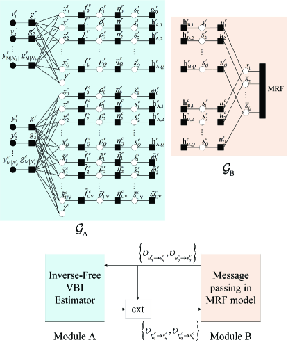
Figure 7: Module A and Module B of the Turbo-IF-VBI-E Step and messages flow between two modules.

Before elaborating on Module A and Module B, we define two factor nodes associated with turbo iteration,

$$\textrm{h}_{\textrm{A},q}^{r} \triangleq\upsilon_{u_{q}^{r}\rightarrow s_{q}^{r}}\left(s_{q}^{r}\right) \textrm{h}_{\textrm{A},q}^{c} \triangleq\upsilon_{u_{q}^{c}\rightarrow s_{q}^{c}}\left(s_{q}^{c}\right),$$ (27)

$$\textrm{h}_{\textrm{B},q}^{r} \triangleq\upsilon_{\eta_{q}^{r}\rightarrow s_{q}^{r}}\left(s_{q}^{r}\right) \textrm{h}_{\textrm{B},q}^{c} \triangleq\upsilon_{\eta_{q}^{c}\rightarrow s_{q}^{c}}\left(s_{q}^{c}\right),$$

for $q=1,\ldots,Q$. For each turbo iteration, Module A treats $\textrm{h}_{\textrm{A},q}^{r}$ and $\textrm{h}_{\textrm{A},q}^{c}$ as the prior and performs the IF-VBI estimator to calculate the approximate conditional posteriors. Then, Module A passes extrinsic messages to Module B by subtracting the prior information from posterior information, i.e.,

$$\upsilon_{\eta_{q}^{r}\rightarrow s_{q}^{r}}\left(s_{q}^{r}\right) \propto q\left(s_{q}^{r}\right)/\textrm{h}_{\textrm{A},q}^{r},\forall q,$$ (28)

$$\upsilon_{\eta_{q}^{c}\rightarrow s_{q}^{c}}\left(s_{q}^{c}\right) \propto q\left(s_{q}^{c}\right)/\textrm{h}_{\textrm{A},q}^{c},\forall q,$$

where $q\left(s_{q}^{r}\right)$ and $q\left(s_{q}^{c}\right)$ are approximate marginal posteriors obtained in Module A. Similarly, Module B performs message passing over $\mathcal{G_{B}}$ and passes the extrinsic messages to Module A. The two modules iterate until they reach a point of convergence.

IV-C Inverse-Free VBI Estimator (Module A)

We first give an overview of the variational Bayesian inference. For convenience, let $\boldsymbol{v}^{l}$ denote an individual variable in $\boldsymbol{v}$, such as $\boldsymbol{x},\boldsymbol{\rho},\boldsymbol{s},\gamma^{r},\gamma^{c}$. Let $\mathcal{H}\triangleq\left\{l\mid\forall\boldsymbol{v}^{l}\in\boldsymbol{v}\right\}$. The posterior $p\left(\boldsymbol{v}\mid\boldsymbol{y};\boldsymbol{\xi}\right)$ is approximated by the product of some variational distributions,

$$p\left(\boldsymbol{v}\mid\boldsymbol{y};\boldsymbol{\xi}\right)\approx q\left(\boldsymbol{v}\right)=q\left(\boldsymbol{x}\right)q\left(\boldsymbol{\rho}\right)q\left(\boldsymbol{s}\right)q\left(\gamma^{r}\right)q\left(\gamma^{c}\right),$$ (29)

where $q\left(\boldsymbol{v}^{l}\right),l\in\mathcal{H}$ are calculated by maximizing the ELBO (equal to minimizing the KL-divergence). The ELBO is given by

$$L\left(q\right)= \int_{\boldsymbol{v}}q\left(\boldsymbol{v}\right)\ln\dfrac{p\left(\boldsymbol{y},\boldsymbol{v};\boldsymbol{\xi}\right)}{q\left(\boldsymbol{v}\right)}$$

$$= \int_{\boldsymbol{v}}q\left(\boldsymbol{v}\right)\ln\Bigl{(}\dfrac{p\left(\boldsymbol{y}\mid\boldsymbol{x},\gamma^{r},\gamma^{c};\boldsymbol{\xi}\right)}{q\left(\boldsymbol{v}\right)}$$

$$\hskip 28.45274ptp\left(\boldsymbol{x}\mid\boldsymbol{\rho}\right)p\left(\boldsymbol{\rho}\mid\boldsymbol{s}\right)p\left(\boldsymbol{s}\right)p\left(\gamma^{r}\right)p\left(\gamma^{c}\right)\Bigr{)}.$$ (30)

The authors in [18] have proved that a stationary solution, denoted by $q^{*}\left(\boldsymbol{v}\right)$, could be found via alternately optimize each variational distribution $q\left(\boldsymbol{v}^{l}\right),\forall l\in\mathcal{H}$. Specifically, for given $q\left(\boldsymbol{v}^{k}\right),\forall k\neq l$, the optimal $q\left(\boldsymbol{v}^{l}\right)$ that maximizes the ELBO can be obtained as

$$q\left(\boldsymbol{v}^{l}\right)=\frac{\exp\left(\left\langle\ln p\left(\boldsymbol{v},\boldsymbol{y}\right)\right\rangle_{\prod_{k\neq l}q\left(\boldsymbol{v}^{k}\right)}\right)}{\int_{\boldsymbol{v}^{l}}\exp\left(\left\langle\ln p\left(\boldsymbol{v},\boldsymbol{y}\right)\right\rangle_{\prod_{k\neq l}q\left(\boldsymbol{v}^{k}\right)}\right)},$$ (31)

where $\left\langle\cdot\right\rangle_{\prod_{k\neq l}q\left(\boldsymbol{v}^{k}\right)}$ denotes an expectation w.r.t the distributions $q\left(\boldsymbol{v}^{k}\right)$ for $k\neq l$. According to (31), the update of $q\left(\boldsymbol{x}\right)$ is a Gaussian distribution with its mean and covariance matrix respectively given by

$$\boldsymbol{\mu} =\boldsymbol{\Sigma}\boldsymbol{\Phi}\left(\boldsymbol{\vartheta}\right)^{H}\left\langle\mathbf{\Gamma}\right\rangle\boldsymbol{y},$$ (32)

$$\boldsymbol{\Sigma} =\left(\boldsymbol{\Phi}\left(\boldsymbol{\vartheta}\right)^{H}\left\langle\mathbf{\Gamma}\right\rangle\boldsymbol{\Phi}\left(\boldsymbol{\vartheta}\right)+\textrm{diag}\left(\left\langle\boldsymbol{\rho}\right\rangle\right)\right)^{-1},$$

where $\boldsymbol{\Gamma}\triangleq\textrm{BlockDiag}\left(\gamma^{r}\mathbf{I}_{M\left|\mathcal{N}_{b}\right|},\gamma^{c}\mathbf{I}_{M\left|\mathcal{N}_{u}\right|}\right)$ is a diagonal matrix. Note that the update of $\boldsymbol{\Sigma}$ involves a matrix inverse, whose computational complexity is $\Theta\left(\left(1+Q+UV\right)^{3}\right)$. Therefore, the algorithm is very time-consuming since $\left(1+Q+UV\right)$ is large.

To overcome this challenge, we follow the IF-SBL approach in [24] and avoid the matrix inverse via maximizing a relaxed ELBO instead.

Specifically, a lower bound of the likelihood function $p\left(\boldsymbol{y}\mid\boldsymbol{x},\gamma^{r},\gamma^{c};\boldsymbol{\xi}\right)$ can be obtained as

$$p\left(\boldsymbol{y}\mid\boldsymbol{x},\gamma^{r},\gamma^{c};\boldsymbol{\xi}\right)$$

$$= \dfrac{\det\left(\boldsymbol{\Gamma}\right)}{\pi^{M\left(\left|\mathcal{N}_{b}\right|+\left|\mathcal{N}_{u}\right|\right)}}\exp\left(-\left(\boldsymbol{y}-\boldsymbol{\Phi}\left(\boldsymbol{\vartheta}\right)\boldsymbol{x}\right)^{H}\boldsymbol{\Gamma}\left(\boldsymbol{y}-\boldsymbol{\Phi}\left(\boldsymbol{\vartheta}\right)\boldsymbol{x}\right)\right)$$

$$\geq \dfrac{\det\left(\boldsymbol{\Gamma}\right)}{\pi^{M\left(\left|\mathcal{N}_{b}\right|+\left|\mathcal{N}_{u}\right|\right)}}\exp\left(-g\left(\boldsymbol{x},\boldsymbol{w}\right)\right)\triangleq F\left(\boldsymbol{y},\boldsymbol{x},\boldsymbol{w},\gamma^{r},\gamma^{c};\boldsymbol{\xi}\right),$$ (33)

where the inequality in (33) follows from Lemma 1 in [24], and

$$g\left(\boldsymbol{x},\boldsymbol{w}\right)\triangleq \left(\boldsymbol{y}-\boldsymbol{\Phi}\left(\boldsymbol{\vartheta}\right)\boldsymbol{w}\right)^{H}\boldsymbol{\Gamma}\left(\boldsymbol{y}-\boldsymbol{\Phi}\left(\boldsymbol{\vartheta}\right)\boldsymbol{w}\right)$$

$$+2\mathfrak{Re}\left\{\left(\boldsymbol{x}-\boldsymbol{w}\right)^{H}\boldsymbol{\Phi}\left(\boldsymbol{\vartheta}\right)^{H}\boldsymbol{\Gamma}\left(\boldsymbol{\Phi}\left(\boldsymbol{\vartheta}\right)\boldsymbol{w}-\boldsymbol{y}\right)\right\}$$

$$+\left(\boldsymbol{x}-\boldsymbol{w}\right)^{H}\boldsymbol{\Gamma}\mathbf{T}\left(\boldsymbol{x}-\boldsymbol{w}\right).$$ (34)

Here $\mathbf{T}$ needs to satisfy $\mathbf{T}\succeq\boldsymbol{\Phi}\left(\boldsymbol{\vartheta}\right)^{H}\boldsymbol{\Phi}\left(\boldsymbol{\vartheta}\right)$. And a good choice of $\mathbf{T}$ is

$$\mathbf{T}=\textrm{BlockDiag}\left(T^{r}\mathbf{I}_{M\left|\mathcal{N}_{b}\right|},T^{c}\mathbf{I}_{M\left|\mathcal{N}_{u}\right|}\right),$$ (35)

with

$$T^{r} \triangleq\textrm{$\lambda_{max}$}\left(\boldsymbol{\Phi}^{r}\left(\boldsymbol{\vartheta}\right)^{H}\boldsymbol{\Phi}^{r}\left(\boldsymbol{\vartheta}\right)\right),$$

$$T^{c} \textrm{$\triangleq\lambda_{max}$}\left(\boldsymbol{\Phi}^{c}\left(\boldsymbol{\vartheta}\right)^{H}\boldsymbol{\Phi}^{c}\left(\boldsymbol{\vartheta}\right)\right),$$

where $\textrm{$\lambda_{max}$}\left(\cdot\right)$ denotes the biggest eigenvalue of a matrix. In this case, $\mathbf{T}$ is a diagonal matrix.

Substituting (33) into (30), we obtain a relaxed ELBO as

$$L\left(q\right)\geq\widetilde{L}\left(q,\boldsymbol{w}\right)\triangleq\int_{\boldsymbol{v}}q\left(\boldsymbol{v}\right)\ln\dfrac{G\left(\boldsymbol{y},\boldsymbol{v},\boldsymbol{w};\boldsymbol{\xi}\right)}{q\left(\boldsymbol{v}\right)},$$ (36)

where

$$G\left(\boldsymbol{y},\boldsymbol{v},\boldsymbol{w};\boldsymbol{\xi}\right)$$ (37)

$$= F\left(\boldsymbol{y},\boldsymbol{x},\boldsymbol{w},\gamma^{r},\gamma^{c};\boldsymbol{\xi}\right)p\left(\boldsymbol{x}\mid\boldsymbol{\rho}\right)p\left(\boldsymbol{\rho}\mid\boldsymbol{s}\right)p\left(\boldsymbol{s}\right)p\left(\gamma^{r}\right)p\left(\gamma^{c}\right).$$

Now we maximize the relaxed ELBO $\widetilde{L}\left(q,\boldsymbol{w}\right)$ w.r.t $q\left(\boldsymbol{v}\right)$ and $\boldsymbol{w}$ based on the EM method. Specifically, for given parameters $\boldsymbol{w}$, optimize each variational distribution $q\left(\boldsymbol{v}^{l}\right),\forall l\in\mathcal{H}$ alternately. On the other hand, for given $q\left(\boldsymbol{v}\right)$, maximize $\widetilde{L}\left(q,\boldsymbol{w}\right)$ w.r.t $\boldsymbol{w}$.

IV-C1 Update of $q\left(\boldsymbol{v}\right)$

Using (31) and ignoring the terms that are not depend on $\boldsymbol{x}$, $q\left(\boldsymbol{x}\right)$ can be derived as

$$\ln q\left(\boldsymbol{x}\right)\propto \ln F\left(\boldsymbol{y},\boldsymbol{x},\boldsymbol{w},\gamma^{r},\gamma^{c};\boldsymbol{\xi}\right)+\ln p\left(\boldsymbol{x}\mid\boldsymbol{\rho}\right)$$

$$\propto -\boldsymbol{x}^{H}\left(\left\langle\boldsymbol{\Gamma}\right\rangle\mathbf{T}+\textrm{diag}\left(\left\langle\boldsymbol{\rho}\right\rangle\right)\right)\boldsymbol{x}$$

$$+2\mathfrak{Re}\left\{\boldsymbol{x}^{H}\boldsymbol{\Phi}\left(\boldsymbol{\vartheta}\right)^{H}\left\langle\boldsymbol{\Gamma}\right\rangle\left(\boldsymbol{y}-\boldsymbol{\Phi}\left(\boldsymbol{\vartheta}\right)\boldsymbol{w}\right)\right\}$$

$$+2\mathfrak{Re}\left\{\boldsymbol{x}^{H}\left\langle\boldsymbol{\Gamma}\right\rangle\mathbf{T}\boldsymbol{w}\right\}$$

$$\propto \ln\mathcal{CN}\left(\boldsymbol{x};\boldsymbol{\mu},\boldsymbol{\Sigma}\right).$$ (38)

where the posterior mean and covariance matrix are respectively given by

$$\boldsymbol{\mu} =\boldsymbol{\Sigma}\left(\boldsymbol{\Phi}\left(\boldsymbol{\vartheta}\right)^{H}\left\langle\boldsymbol{\Gamma}\right\rangle\left(\boldsymbol{y}-\boldsymbol{\Phi}\left(\boldsymbol{\vartheta}\right)\boldsymbol{w}\right)+\left\langle\boldsymbol{\Gamma}\right\rangle\mathbf{T}\boldsymbol{w}\right),$$ (39)

$$\boldsymbol{\Sigma} =\left(\left\langle\boldsymbol{\Gamma}\right\rangle\mathbf{T}+\textrm{diag}\left(\left\langle\boldsymbol{\rho}\right\rangle\right)\right)^{-1}.$$

Note that $\boldsymbol{\Sigma}$ is calculated by a diagonal matrix inverse and $\boldsymbol{\mu}$ is computed by the matrix-vector product. Therefore, the computational complexity of $q\left(\boldsymbol{x}\right)$ is significantly reduced.

The update of $q\left(\boldsymbol{\rho}\right)$, $q\left(\boldsymbol{s}\right)$, $q\left(\gamma^{r}\right)$, and $q\left(\gamma^{c}\right)$ can be derived in the same way. Please refer to the Turbo-VBI algorithm in [18] for the expressions of these variational distributions.

IV-C2 Update of $\boldsymbol{w}$

Submitting $q\left(\boldsymbol{v};\boldsymbol{w}^{\textrm{old}}\right)$ into $\widetilde{L}\left(q,\boldsymbol{w}\right)$, an estimate of $\boldsymbol{w}$ can be obtained as

$$\boldsymbol{w}^{\textrm{new}}=\arg\max_{\boldsymbol{w}}\left\langle\ln G\left(\boldsymbol{y},\boldsymbol{v},\boldsymbol{w};\boldsymbol{\xi}\right)\right\rangle_{q\left(\boldsymbol{v};\boldsymbol{w}^{\textrm{old}}\right)}.$$ (40)

The gradient of $\left\langle\ln G\left(\boldsymbol{y},\boldsymbol{v},\boldsymbol{w};\boldsymbol{\xi}\right)\right\rangle_{q\left(\boldsymbol{v};\boldsymbol{w}^{\textrm{old}}\right)}$ w.r.t $\boldsymbol{w}$ is given by

$$\frac{\partial\left\langle\ln G\left(\boldsymbol{y},\boldsymbol{v},\boldsymbol{w};\boldsymbol{\xi}\right)\right\rangle_{q\left(\boldsymbol{v};\boldsymbol{w}^{\textrm{old}}\right)}}{\partial\boldsymbol{w}}$$

$$= \left\langle\boldsymbol{\Gamma}\right\rangle\left(\mathbf{T}-\boldsymbol{\Phi}\left(\boldsymbol{\vartheta}\right)^{H}\boldsymbol{\Phi}\left(\boldsymbol{\vartheta}\right)\right)\left(\boldsymbol{\mu}-\boldsymbol{w}\right).$$ (41)

By setting the gradient to zero, we have

$$\boldsymbol{w}^{\textrm{new}}=\boldsymbol{\mu}.$$ (42)

IV-D Message Passing in MRF (Module B)

In $\mathcal{G}_{B}$, the sub factor graphs associated with $\boldsymbol{s}^{r}$ and $\boldsymbol{s}^{c}$ are coupled together via the variable nodes $\left\{\overline{s}_{q}\right\}$. Therefore, they exchange messages to obtain more accurate estimates for $\boldsymbol{s}^{r}$ and $\boldsymbol{s}^{c}$. In other words, the sensing and communication functionalities assist each other when performing message passing. We follow the sum-product rule to derive the message passing algorithm over $\mathcal{G}_{B}$. To simplify the notation, $\pi_{q}^{r}$, $\pi_{q}^{c}$, $\pi_{q}^{r,in}$, and $\pi_{q}^{c,in}$ are used to abbreviate $\textrm{h}_{\textrm{A},q}^{r}\left(s_{q}^{r}=1\right)$, $\textrm{h}_{\textrm{A},q}^{c}\left(s_{q}^{c}=1\right)$, $\textrm{h}_{\textrm{B},q}^{r}\left(s_{q}^{r}=1\right)$, and $\textrm{h}_{\textrm{B},q}^{c}\left(s_{q}^{c}=1\right)$, respectively, for $q=1,\ldots,Q$. The message from the factor nodes $u_{q}^{r}$ and $u_{q}^{c}$ to the variable node $\overline{s}_{q}$ are respectively given by

$$\nu_{u_{q}^{r}\rightarrow\overline{s}_{q}} \propto\sum_{s_{q}^{r}}\nu_{s_{q}^{r}\rightarrow u_{q}^{r}}\times u_{q}^{r}\left(s_{q}^{r},\overline{s}_{q}\right)$$ (43)

$$\propto\pi_{u_{q}^{r}\rightarrow\overline{s}_{q}}\delta\left(\overline{s}_{q}-1\right)+\left(1-\pi_{u_{q}^{r}\rightarrow\overline{s}_{q}}\right)\delta\left(\overline{s}_{q}+1\right),$$

$$\nu_{u_{q}^{c}\rightarrow\overline{s}_{q}} \propto\sum_{s_{q}^{c}}\nu_{s_{q}^{c}\rightarrow u_{q}^{c}}\times u_{q}^{c}\left(s_{q}^{c},\overline{s}_{q}\right)$$

$$\propto\pi_{u_{q}^{c}\rightarrow\overline{s}_{q}}\delta\left(\overline{s}_{q}-1\right)+\left(1-\pi_{u_{q}^{c}\rightarrow\overline{s}_{q}}\right)\delta\left(\overline{s}_{q}+1\right),$$

where

$$\pi_{u_{q}^{r}\rightarrow\overline{s}_{q}} =\left(1+\tfrac{1-\pi_{q}^{r,in}}{1+2\lambda_{q}^{r}\pi_{q}^{r,in}-\lambda_{q}^{r}-\pi_{q}^{r,in}}\right)^{-1},$$

$$\pi_{u_{q}^{c}\rightarrow\overline{s}_{q}} =\left(1+\tfrac{1-\pi_{q}^{c,in}}{1+2\lambda_{q}^{c}\pi_{q}^{c,in}-\lambda_{q}^{c}-\pi_{q}^{c,in}}\right)^{-1}.$$

Consider the variable node $\overline{s}_{q}$ and define the index set of its neighbors as $\mathcal{N}_{q}\triangleq\left\{q_{l},q_{r},q_{t},q_{b}\right\}$, where the left, right, top, and bottom neighbors are $\overline{s}_{q_{l}}\triangleq\overline{s}_{q-H}$, $\overline{s}_{q_{r}}\triangleq\overline{s}_{q+H}$, $\overline{s}_{q_{t}}\triangleq\overline{s}_{q-1}$, and $\overline{s}_{q_{b}}\triangleq\overline{s}_{q+1}$, respectively. Then the input messages of $\overline{s}_{q}$ from the left, right, top, and bottom, denoted by $\nu_{q}^{l}$, $\nu_{q}^{r}$, $\nu_{q}^{t}$, and $\nu_{q}^{b}$, are Bernoulli distributions, where $\nu_{q}^{l}$ can be calculated as

$$\nu_{q}^{l} \propto\sum_{\overline{s}_{q_{l}}}\nu_{u_{q_{l}}^{r}\rightarrow\overline{s}_{q_{l}}}\nu_{u_{q_{l}}^{c}\rightarrow\overline{s}_{q_{l}}}\prod_{k\in\left\{l,t,b\right\}}\nu_{q_{l}}^{k}\psi\left(\overline{s}_{q_{l}}\right)\varphi\left(\overline{s}_{q},\overline{s}_{q_{l}}\right)$$

$$\propto\kappa_{q}^{l}\delta\left(\overline{s}_{q}-1\right)+(1-\kappa_{q}^{l})\delta\left(\overline{s}_{q}+1\right),$$ (44)

where $\kappa_{q}^{l}$ is given in (45) at the top of the next page.

$$\kappa_{q}^{l}=\dfrac{\pi_{u_{q_{l}}^{r}\rightarrow\overline{s}_{q_{l}}}\pi_{u_{q_{l}}^{c}\rightarrow\overline{s}_{q_{l}}}\prod_{k\in\left\{l,t,b\right\}}\kappa_{q_{l}}^{k}e^{-\alpha_{q_{l}}+\beta_{q,q_{l}}}+\left(1-\pi_{u_{q_{l}}^{r}\rightarrow\overline{s}_{q_{l}}}\right)\left(1-\pi_{u_{q_{l}}^{c}\rightarrow\overline{s}_{q_{l}}}\right)\prod_{k\in\left\{l,t,b\right\}}\left(1-\kappa_{q_{l}}^{k}\right)e^{\alpha_{q_{l}}-\beta_{q,q_{l}}}}{\left(e^{\beta_{q,q_{l}}}+e^{-\beta_{q,q_{l}}}\right)\left(\pi_{u_{q_{l}}^{r}\rightarrow\overline{s}_{q_{l}}}\pi_{u_{q_{l}}^{c}\rightarrow\overline{s}_{q_{l}}}e^{-\alpha_{q_{l}}}\prod_{k\in\left\{l,t,b\right\}}\kappa_{q_{l}}^{k}+\left(1-\pi_{u_{q_{l}}^{r}\rightarrow\overline{s}_{q_{l}}}\right)\left(1-\pi_{u_{q_{l}}^{c}\rightarrow\overline{s}_{q_{l}}}\right)e^{\alpha_{q_{l}}}\prod_{k\in\left\{l,t,b\right\}}\left(1-\kappa_{q_{l}}^{k}\right)\right)}.$$ (45)

The other input messages of $\overline{s}_{q}$, i.e., $\nu_{q}^{r}$, $\nu_{q}^{t}$ and $\nu_{q}^{b}$, have a similar form to $\nu_{q}^{l}$.

The message from the variable node $\overline{s}_{q}$ to the factor node $u_{q}^{r}$ is given by

$$\nu_{\overline{s}_{q}\rightarrow u_{q}^{r}} \propto\nu_{u_{q}^{c}\rightarrow\overline{s}_{q}}\Pi_{k\in\left\{l,r,t,b\right\}}\nu_{q}^{k}\psi\left(\overline{s}_{q}\right)$$ (46)

$$\propto\pi_{\overline{s}_{q}\rightarrow u_{q}^{r}}\delta\left(\overline{s}_{q}-1\right)+\left(1-\pi_{\overline{s}_{q}\rightarrow u_{q}^{r}}\right)\delta\left(\overline{s}_{q}+1\right),$$

where $\pi_{\overline{s}_{q}\rightarrow u_{q}^{r}}$ is given in (47) at the top of the next page.

$$\pi_{\overline{s}_{q}\rightarrow u_{q}^{r}}=\frac{e^{-\alpha_{q}}\pi_{u_{q}^{c}\rightarrow\overline{s}_{q}}\Pi_{k\in\left\{l,r,t,b\right\}}\kappa_{q}^{k}}{e^{-\alpha_{q}}\pi_{u_{q}^{c}\rightarrow\overline{s}_{q}}\Pi_{k\in\left\{l,r,t,b\right\}}\kappa_{q}^{k}+e^{\alpha_{q}}\left(1-\pi_{u_{q}^{c}\rightarrow\overline{s}_{q}}\right)\Pi_{k\in\left\{l,r,t,b\right\}}\left(1-\kappa_{q}^{k}\right)}.$$ (47)

 

The message from the factor node $u_{q}^{r}$ back to the variable node $s_{q}^{r}$ is given by

$$\nu_{u_{q}^{r}\rightarrow s_{q}^{r}} \propto\sum_{\overline{s}_{q}}\nu_{\overline{s}_{q}\rightarrow u_{q}^{r}}\times u_{q}^{r}\left(s_{q}^{r},\overline{s}_{q}\right)$$

$$\propto\pi_{q}^{r}\delta\left(s_{q}^{r}-1\right)+\left(1-\pi_{q}^{r}\right)\delta\left(s_{q}^{r}+1\right),$$ (48)

where $\pi_{q}^{r}=\pi_{\overline{s}_{q}\rightarrow u_{q}^{r}}\lambda_{q}^{r}$. Similarly, the message from the factor node $u_{q}^{c}$ back to the variable node $s_{q}^{c}$ is given by

$$\nu_{u_{q}^{c}\rightarrow s_{q}^{c}}=\pi_{q}^{c}\delta\left(s_{q}^{c}-1\right)+\left(1-\pi_{q}^{c}\right)\delta\left(s_{q}^{c}+1\right),$$ (49)

where $\pi_{q}^{c}=\pi_{\overline{s}_{q}\rightarrow u_{q}^{c}}\lambda_{q}^{c}$.

The approximate marginal posterior $q\left(\overline{\boldsymbol{s}}\mid\boldsymbol{y};\boldsymbol{\xi}\right)$ can be obtained as

$$q\left(\overline{\boldsymbol{s}}\mid\boldsymbol{y};\boldsymbol{\xi}\right) \propto\prod_{q}\nu_{u_{q}^{r}\rightarrow\overline{s}_{q}}\times\nu_{\overline{s}_{q}\rightarrow u_{q}^{r}}$$ (50)

$$\propto\prod_{q}\left(\pi_{\overline{s}_{q}}\delta\left(\overline{s}_{q}-1\right)+\left(1-\pi_{\overline{s}_{q}}\right)\delta\left(\overline{s}_{q}+1\right)\right),$$

where $\pi_{\overline{s}_{q}}=\frac{\pi_{u_{q}^{r}\rightarrow\overline{s}_{q}}\pi_{\overline{s}_{q}\rightarrow u_{q}^{r}}}{\pi_{u_{q}^{r}\rightarrow\overline{s}_{q}}\pi_{\overline{s}_{q}\rightarrow u_{q}^{r}}+\left(1-\pi_{u_{q}^{r}\rightarrow\overline{s}_{q}}\right)\left(\pi_{\overline{s}_{q}\rightarrow u_{q}^{r}}\right)},\forall q$.

IV-E Turbo-IF-VBI-M Step

Since there is no close-form expression of $\ln p\left(\boldsymbol{y},\boldsymbol{\xi}\right)$, it is challenging to directly solve the maximization problem in (26). To get around this problem, one common solution is to construct a surrogate function of $\ln p\left(\boldsymbol{y},\boldsymbol{\xi}\right)$ and maximize the surrogate function with respect to $\boldsymbol{\xi}$. Specifically, in the $t\textrm{-th}$ iteration, the surrogate function inspired by the EM method is given by

$$Q\left(\boldsymbol{\xi};\boldsymbol{\xi}^{\left(t\right)}\right) =\sum_{\overline{\boldsymbol{s}}}\int_{\boldsymbol{v}}q^{\left(t\right)}\left(\boldsymbol{v},\overline{\boldsymbol{s}}\right)\ln\frac{p\left(\boldsymbol{y},\boldsymbol{v},\overline{\boldsymbol{s}};\boldsymbol{\xi}\right)}{q^{\left(t\right)}\left(\boldsymbol{v},\overline{\boldsymbol{s}}\right)}+\ln p\left(\boldsymbol{\vartheta}\right)$$

$$=Q_{\boldsymbol{\vartheta}}\left(\boldsymbol{\vartheta};\boldsymbol{\xi}^{\left(t\right)}\right)+Q_{\boldsymbol{\zeta}}\left(\boldsymbol{\zeta};\boldsymbol{\xi}^{\left(t\right)}\right)+C,$$ (51)

where

$$Q_{\boldsymbol{\vartheta}}\left(\boldsymbol{\vartheta};\boldsymbol{\xi}^{\left(t\right)}\right)= -\left(\boldsymbol{y}-\boldsymbol{\Phi}\left(\boldsymbol{\vartheta}\right)\boldsymbol{\mu}^{\left(t\right)}\right)^{H}\boldsymbol{\Gamma}\left(\boldsymbol{y}-\boldsymbol{\Phi}\left(\boldsymbol{\vartheta}\right)\boldsymbol{\mu}^{\left(t\right)}\right)$$

$$-\textrm{tr}\left(\boldsymbol{\Gamma}\boldsymbol{\Phi}\left(\boldsymbol{\vartheta}\right)\boldsymbol{\Sigma}^{\left(t\right)}\boldsymbol{\Phi}\left(\boldsymbol{\vartheta}\right)^{H}\right)+\ln p\left(\boldsymbol{\vartheta}\right),$$

$$Q_{\boldsymbol{\zeta}}\left(\boldsymbol{\zeta};\boldsymbol{\xi}^{\left(t\right)}\right)= \mathbb{E}_{q\left(\overline{\boldsymbol{s}}\mid\boldsymbol{y};\boldsymbol{\xi}^{\left(t\right)}\right)}\left\{\ln p\left(\overline{\boldsymbol{s}};\boldsymbol{\zeta}\right)\right\},$$ (52)

where $\boldsymbol{\mu}^{\left(t\right)}$ and $\boldsymbol{\Sigma}^{\left(t\right)}$ are approximate posterior mean and covariance matrix of $\boldsymbol{x}$ obtained in (39), $q^{\left(t\right)}\left(\boldsymbol{v},\overline{\boldsymbol{s}}\right)\triangleq q\left(\boldsymbol{v}\mid\boldsymbol{y};\boldsymbol{\xi}^{\left(t\right)}\right)q\left(\overline{\boldsymbol{s}}\mid\boldsymbol{y};\boldsymbol{\xi}^{\left(t\right)}\right)$, and $C$ is a constant. At the current iterate $\boldsymbol{\xi}^{\left(t\right)}$, the surrogate function and its gradient satisfy the following properties:

$$Q\left(\boldsymbol{\xi};\boldsymbol{\xi}^{\left(t\right)}\right) \leq\ln p\left(\boldsymbol{y},\boldsymbol{\xi}\right),\forall\boldsymbol{\xi}$$ (53a)

$$Q\left(\boldsymbol{\xi}^{\left(t\right)};\boldsymbol{\xi}^{\left(t\right)}\right) =\ln p\left(\boldsymbol{y},\boldsymbol{\xi}^{\left(t\right)}\right),$$ (53b)

$$\frac{\partial Q\left(\boldsymbol{\xi}^{\left(t\right)};\boldsymbol{\xi}^{\left(t\right)}\right)}{\partial\boldsymbol{\xi}} =\frac{\partial\ln p\left(\boldsymbol{y},\boldsymbol{\xi}^{\left(t\right)}\right)}{\partial\boldsymbol{\xi}}.$$ (53c)

Maximizing $Q\left(\boldsymbol{\xi};\boldsymbol{\xi}^{\left(t\right)}\right)$ is equal to solve the following two subproblems:

$$\boldsymbol{\vartheta}^{\left(t+1\right)} =\underset{\boldsymbol{\vartheta}}{\arg\max}Q_{\boldsymbol{\vartheta}}\left(\boldsymbol{\vartheta};\boldsymbol{\xi}^{\left(t\right)}\right),$$ (54a)

$$\boldsymbol{\zeta}^{\left(t+1\right)} =\underset{\boldsymbol{\zeta}}{\arg\max}Q_{\boldsymbol{\zeta}}\left(\boldsymbol{\zeta};\boldsymbol{\xi}^{\left(t\right)}\right).$$ (54b)

IV-E1 Update of $\boldsymbol{\vartheta}$

It is difficult to find the global optimal solution to the subproblem in (54a) because the function $Q_{\boldsymbol{\vartheta}}\left(\boldsymbol{\vartheta};\boldsymbol{\xi}^{\left(t\right)}\right)$ is non-convex. Using the gradient ascent method, we have

$$\boldsymbol{r}^{\left(t+1\right)} =\boldsymbol{r}^{\left(t\right)}+\varepsilon_{r}^{\left(t\right)}\frac{\partial Q_{\boldsymbol{\vartheta}}\left(\boldsymbol{r}^{\left(t\right)},\boldsymbol{p}_{u}^{\left(t\right)},\tau_{o}^{\left(t\right)};\boldsymbol{\xi}^{\left(t\right)}\right)}{\partial\boldsymbol{r}},$$ (55)

$$\boldsymbol{p}_{u}^{\left(t+1\right)} =\boldsymbol{p}_{u}^{\left(t\right)}+\varepsilon_{p}^{\left(t\right)}\frac{\partial Q_{\boldsymbol{\vartheta}}\left(\boldsymbol{r}^{\left(t+1\right)},\boldsymbol{p}_{u}^{\left(t\right)},\tau_{o}^{\left(t\right)};\boldsymbol{\xi}^{\left(t\right)}\right)}{\partial\boldsymbol{p}_{u}},$$ (56)

$$\tau_{o}^{\left(t+1\right)} =\tau_{o}^{\left(t\right)}+\varepsilon_{\tau}^{\left(t\right)}\frac{\partial Q_{\boldsymbol{\vartheta}}\left(\boldsymbol{r}^{\left(t+1\right)},\boldsymbol{p}_{u}^{\left(t+1\right)},\tau_{o}^{\left(t\right)};\boldsymbol{\xi}^{\left(t\right)}\right)}{\partial\tau_{o}},$$ (57)

where $\varepsilon_{r}^{\left(t\right)}$, $\varepsilon_{p}^{\left(t\right)}$, and $\varepsilon_{\tau}^{\left(t\right)}$ are step sizes determined by the Armijo rule.

IV-E2 Update of $\boldsymbol{\zeta}$

Recalling (52) and (20), we find that the partition function $Z\left(\boldsymbol{\zeta}\right)$ is computationally intractable due to its exponential complexity. Therefore, it is very difficult to directly apply the gradient ascent method to solve the subproblem in (54b). To make the subproblem solvable, a pseudo-likelihood function is introduced to approximate the MRF prior,

$$\textrm{PL}\left(\overline{\boldsymbol{s}};\boldsymbol{\zeta}\right) =\prod_{q\in\mathcal{S}\setminus\partial\mathcal{S}}p\left(\overline{s}_{q}\mid\overline{s}_{q-H},\overline{s}_{q+H},\overline{s}_{q-1},\overline{s}_{q+1}\right)$$ (58)

$$=\prod_{q\in\mathcal{S}\setminus\partial\mathcal{S}}\frac{\exp\left(-\alpha_{q}\overline{s}_{q}+\sum_{i\in\mathcal{N}_{q}}\beta_{iq}\overline{s}_{i}\overline{s}_{q}\right)}{\sum_{\overline{s}_{q}}\exp\left(-\alpha_{q}\overline{s}_{q}+\sum_{i\in\mathcal{N}_{q}}\beta_{iq}\overline{s}_{i}\overline{s}_{q}\right)},$$

where $\mathcal{S}\triangleq\left\{1,\ldots,Q\right\}$ is the index set of variable nodes in the MRF model and $\partial\mathcal{S}$ is the index set of nodes at the boundaries of $\mathcal{S}$. The authors in [25] proved the consistency of the maximum pseudo-likelihood estimate for large $H$ and $W$. In other words, the global optimal solution of maximizing $\ln\textrm{PL}\left(\overline{\boldsymbol{s}};\boldsymbol{\zeta}\right)$ converges to the global optimal of maximizing $\ln p\left(\boldsymbol{s};\boldsymbol{\zeta}\right)$ as $H,W\rightarrow\infty$. Therefore, for large $H$ and $W$, by replacing the likelihood $p\left(\overline{\boldsymbol{s}};\boldsymbol{\zeta}\right)$ in $Q_{\boldsymbol{\zeta}}\left(\boldsymbol{\zeta};\boldsymbol{\xi}^{\left(t\right)}\right)$ with the pseudo-likelihood, we obtain a good approximation to the subproblem as

$$\boldsymbol{\zeta}^{\left(t+1\right)} =\underset{\boldsymbol{\zeta}}{\arg\max}\widetilde{Q}_{\boldsymbol{\zeta}}\left(\boldsymbol{\zeta};\boldsymbol{\xi}^{\left(t\right)}\right)$$

$$=\underset{\boldsymbol{\zeta}}{\arg\max}\mathbb{E}_{q\left(\overline{\boldsymbol{s}}\mid\boldsymbol{y};\boldsymbol{\xi}^{\left(t\right)}\right)}\left\{\ln\textrm{PL}\left(\overline{\boldsymbol{s}};\boldsymbol{\zeta}\right)\right\}.$$ (59)

The gradients of $\widetilde{Q}_{\boldsymbol{\zeta}}\left(\boldsymbol{\zeta};\boldsymbol{\xi}^{\left(t\right)}\right)$ w.r.t. $\alpha_{q}$ and $\beta_{pq}$ are respectively given in (60) and (61) at the top of the next page, where $p,q\in\mathcal{S}\setminus\partial\mathcal{S}$ and $p\in\mathcal{N}_{q}$.

$$\frac{\partial\widetilde{Q}_{\boldsymbol{\zeta}}\left(\boldsymbol{\zeta};\boldsymbol{\xi}^{\left(t\right)}\right)}{\partial\alpha_{q}}=\mathbb{E}_{q\left(\overline{\boldsymbol{s}}\mid\boldsymbol{y};\boldsymbol{\xi}^{\left(t\right)}\right)}\left\{-\overline{s}_{q}+\frac{\exp\left(2\sum_{i\in\mathcal{N}_{q}}\beta_{iq}\overline{s}_{i}\right)-\exp\left(2\alpha_{q}\right)}{\exp\left(2\sum_{i\in\mathcal{N}_{q}}\beta_{iq}\overline{s}_{i}\right)+\exp\left(2\alpha_{q}\right)}\right\},$$ (60)

$$\frac{\partial\widetilde{Q}_{\boldsymbol{\zeta}}\left(\boldsymbol{\zeta};\boldsymbol{\xi}^{\left(t\right)}\right)}{\partial\beta_{pq}}=\mathbb{E}_{q\left(\overline{\boldsymbol{s}}\mid\boldsymbol{y};\boldsymbol{\xi}^{\left(t\right)}\right)}\left\{2\overline{s}_{p}\overline{s}_{q}-\overline{s}_{p}\frac{\exp\left(2\sum_{i\in\mathcal{N}_{q}}\beta_{iq}\overline{s}_{i}\right)-\exp\left(2\alpha_{q}\right)}{\exp\left(2\sum_{i\in\mathcal{N}_{q}}\beta_{iq}\overline{s}_{i}\right)+\exp\left(2\alpha_{q}\right)}-\overline{s}_{q}\frac{\exp\left(2\sum_{i\in\mathcal{N}_{p}}\beta_{ip}\overline{s}_{i}\right)-\exp\left(2\alpha_{p}\right)}{\exp\left(2\sum_{i\in\mathcal{N}_{p}}\beta_{ip}\overline{s}_{i}\right)+\exp\left(2\alpha_{p}\right)}\right\},$$ (61)

 

This time, the gradients can be directly calculated, so the gradient ascent method is feasible without resorting to the time-consuming Monte Carlo method.

We follow the gradient ascent approach, which leads to the following update:

$$\alpha_{q}^{\left(t+1\right)} =\alpha_{q}^{\left(t\right)}+\varepsilon_{\alpha}\frac{\partial\widetilde{Q}_{\boldsymbol{\zeta}}\left(\boldsymbol{\zeta};\boldsymbol{\xi}^{\left(t\right)}\right)}{\partial\alpha_{q}}\mid_{\boldsymbol{\zeta}=\boldsymbol{\zeta}^{\left(t\right)}},$$ (62)

$$\beta_{pq}^{\left(t+1\right)} =\beta_{pq}^{\left(t\right)}+\varepsilon_{\beta}\frac{\partial\widetilde{Q}_{\boldsymbol{\zeta}}\left(\boldsymbol{\zeta};\boldsymbol{\xi}^{\left(t\right)}\right)}{\partial\beta_{pq}}\mid_{\boldsymbol{\zeta}=\boldsymbol{\zeta}^{\left(t\right)}},$$ (63)

where $\varepsilon_{\alpha}$ and $\varepsilon_{\beta}$ are step sizes determined by the Armijo rule.

The complete Turbo-IF-VBI algorithm is summarized in Algorithm 1.

Algorithm 1 Turbo-IF-VBI algorithm

Input: $\boldsymbol{y}$, $\boldsymbol{\Phi}\left(\boldsymbol{\vartheta}\right)$, $p\left(\boldsymbol{\vartheta}\right)$, iteration numbers $I_{in}$ and $I_{out}$, threshold $\epsilon$.

Output: $\boldsymbol{\xi}^{*}$, $\boldsymbol{x}^{*}$, and $\boldsymbol{s}^{*}$.

1:  for ${\color[rgb]{0,0,1}{\color[rgb]{0,0,0}t=1,\cdots,I_{out}}}$ do

2:     Turbo-IF-VBI-E Step:

3:     %Module A: IF-VBI Estimator

4:     Initialize $i_{in}=1$, $\boldsymbol{\xi}$, $\boldsymbol{\pi}$, $\mathbf{T}$, and $\boldsymbol{w}=\boldsymbol{\mu}^{\left(t-1\right)}$, where $\boldsymbol{\mu}^{\left(0\right)}\triangleq\boldsymbol{\Phi}\left(\boldsymbol{\vartheta}\right)^{H}\boldsymbol{y}$.

5:     while not converge and $i_{in}\leq I_{in}$ do

6:        Update $q\left(\boldsymbol{v}\mid\boldsymbol{y};\boldsymbol{\xi}^{\left(t\right)}\right)$, using (39).

7:        Update the parameter $\boldsymbol{w}$, using (42).

8:        $i_{in}=i_{in}+1$.

9:     end while

10:     Calculate the extrinsic information based on (28), send $\upsilon_{\eta_{q}^{r}\rightarrow s_{q}^{r}}$ and $\upsilon_{\eta_{q}^{c}\rightarrow s_{q}^{c}}$ to Module B.

11:     %Module B: Message Passing in MRF

12:     Perform message passing, using (43) - (49).

13:     Calculate the approximate marginal posterior $q\left(\overline{\boldsymbol{s}}\mid\boldsymbol{y};\boldsymbol{\xi}^{\left(t\right)}\right)$, using (50).

14:     Send $\upsilon_{u_{q}^{r}\rightarrow s_{q}^{r}}$ and $\upsilon_{u_{q}^{c}\rightarrow s_{q}^{c}}$ to Module A.

15:     Turbo-IF-VBI-M Step:

16:     Construct the surrogate function $Q\left(\boldsymbol{\xi};\boldsymbol{\xi}^{i}\right)$ in (51).

17:     Update $\boldsymbol{\vartheta}^{i+1}$, using (55) - (57).

18:     Update $\boldsymbol{\zeta}^{i+1}$, using (62) and (63).

19:     if $\left\|\boldsymbol{\xi}^{i+1}-\boldsymbol{\xi}^{i}\right\|\leq\epsilon$ then

20:        break

21:     end if

22:  end for

23:  Output $\boldsymbol{\xi}^{\ast}$, $\boldsymbol{x}^{*}=\boldsymbol{\mu}$, and $s_{i}^{*}=\arg\max_{s_{i}}q\left(s_{i}\mid\boldsymbol{y};\boldsymbol{\xi}^{\ast}\right)$.

IV-F Complexity Analysis

We discuss the computational complexity of the proposed algorithm and other existing algorithms. The computational complexity of the Turbo-IF-VBI algorithm is dominated by the update of $q\left(\boldsymbol{v}\mid\boldsymbol{y};\boldsymbol{\xi}\right)$ in Module A. Specifically, the IF-VBI estimator (Module A) involves some matrix-vector product and diagonal matrix inverse operations in each iteration. Therefore, the computational complexity order of the proposed algorithm is $\mathcal{O}\left(M\left(\left|N_{u}\right|+\left|N_{b}\right|\right)\left(1+Q+UV\right)\right)$ per iteration. The existing sparse Bayesian inference algorithms, such as the Turbo-SBI [9] and Turbo-VBI [18], involve a matrix inverse in each iteration. And the associated computational complexity order of these algorithms is $\mathcal{O}\left(\left(1+Q+UV\right)^{3}\right)$ per iteration, which is much higher than that of the Turbo-IF-VBI algorithm.

V Simulation Results

In this section, we evaluate the performance of our proposed scheme and compare it with some baselines to verify its advantages. The baselines and our proposed scheme are summarized as follows:

• Baseline 1: The orthogonal matching pursuit (OMP) algorithm [26, 27] with a fixed position grid.

• Baseline 2: The Turbo-SBI algorithm [9].

• Baseline 3: The Turbo-IF-VBI algorithm with an i.i.d. prior (the factor graph has no joint support vector $\boldsymbol{\overline{s}}$ and the elements of $\boldsymbol{s}^{r}$ and $\boldsymbol{s}^{c}$ are i.i.d., respectively).

• Proposed: The Turbo-IF-VBI algorithm with the MRF prior.

• Genie-aided method: The genie-aided method uses the proposed scheme based on the assumption that the user location and time offset are perfectly known.

• Proposed without relaxing: This scheme is a minor variation of the proposed scheme. The only different is that Module A directly maximizes the ELBO without constructing a relaxed ELBO. And thus it involves a high-dimensional matrix inverse in each iteration.

Baseline 1 is a classic compressed sensing algorithm. Baseline 2 is the state-of-the-art method based on sparse Bayesian inference. Baseline 3 and our proposed scheme use the same algorithm, i.e., the proposed Turbo-IF-VBI, but with different sparse prior models. The performance gain between baseline 3 and our proposed scheme reflects the gain from utilizing the 2-D joint burst sparsity of the location domain channels.

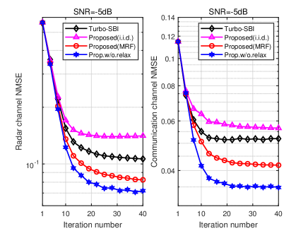
Figure 8: The convergence behavior of different algorithms when $\textrm{SNR}=-5\ \textrm{dB}$.

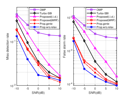
Figure 9: Miss detection rate and false alarm rate of target detection versus SNR.

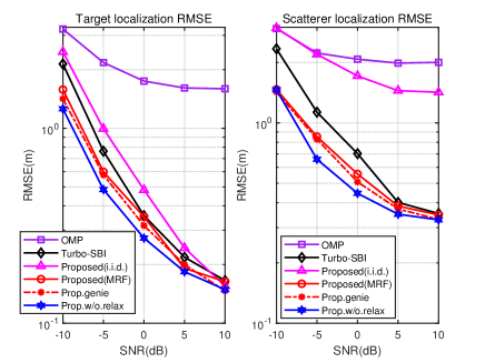
Figure 10: RMSE of target and scatterer localization versus SNR.

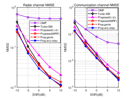
Figure 11: NMSE of radar and communication channel estimation versus SNR.

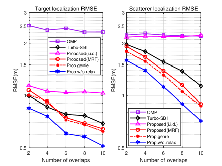
Figure 12: RMSE of target and scatterer localization versus number of overlaps.

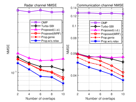
Figure 13: NMSE of radar and communication channel estimation versus number of overlaps.

In the simulations, we consider a $100\text{ m}\times 100\text{ m}$ area with a grid resolution of $5\text{ m}$. The BS is at coordinates $\left[-50\text{ m},0\text{ m}\right]^{T}$ and the mobile user is around coordinates $\left[50\text{ m},0\text{ m}\right]^{T}$ with a random position offset. We assume that the prior distribution of $\boldsymbol{p}_{u}$ is $p^{x}\sim\mathcal{N}\left(50,\sigma_{p}^{2}/2\right)$ and $p^{y}\sim\mathcal{N}\left(0,\sigma_{p}^{2}/2\right)$, where $\sigma_{p}^{2}$ is set as $1$. There are $K=11$ radar targets and $L=13$ communication scatterers within the area. Radar targets and communication scatterers are concentrated on two clusters with different sizes. The number of OFDM subcarriers is $N=1024$, the carrier frequency is $3.5\ \textrm{GHz}$, and the subcarrier interval is $f_{0}=30\text{ kHz}$. Downlink and uplink pilot symbols are generated with random phase under unit power constrains, and they are inserted at intervals of $32$ OFDM subcarriers, i.e., $\left|\mathcal{N}_{b}\right|=32$ and $\left|\mathcal{N}_{u}\right|=32$. The BS is equipped with a ULA of $M=64$ antennas. The time offset $\tau_{o}$ is within $\left[\frac{-2}{B},\frac{2}{B}\right]$, where $B=Nf_{0}$ denotes the total bandwidth. We use the root mean square error (RMSE) as the performance metric for target and scatterer localization and the normalized mean square error (NMSE) as the performance metric for radar and communication channel estimation. Furthermore, we also evaluate the target detection performance in terms of miss detection rate and false alarm rate. To be more specific, $q\left(s_{q}^{r}=1\right)>0.5$ indicates that the BS detects a target lying in the $q\textrm{-th}$ position grid, while $q\left(s_{q}^{r}=1\right)<0.5$ indicates the opposite, where $q\left(s_{q}^{r}=1\right)$ is the posterior probability of $s_{q}^{r}=1$ obtained by the algorithms.

V-A Convergence Behavior

Fig. 9 illustrates the convergence behavior of different algorithms. It can be seen that the proposed Turbo-IF-VBI algorithm converges quickly within 20 iterations. This further implies that the approximate marginal posteriors provided by Turbo-IF-VBI-E Step are accurate enough that they have little effect on the convergence performance of the whole algorithm. However, the proposed algorithm with an i.i.d. prior converges to a poor stationary point, while the proposed algorithm with the MRF prior finds a better solution. It verifies the advantage of the MRF prior in terms of convergence performance.

V-B Impact of Signal to Noise Ratio (SNR)

In Fig. 9 - 11, we focus on how the SNR affects sensing/estimation performance. To be more specific, Fig. 9 shows the miss detection rate and false alarm rate of target detection, Fig. 11 shows the RMSE of target and scatterer localization, and Fig. 11 shows the NMSE performance of radar and communication channel estimation. The performance of all schemes improves as the SNR increases, except for the OMP. Since the OMP uses a fixed position grid, the performance of the algorithm is limited by the grid resolution in the high SNR region. In the low SNR region, the proposed algorithm with the MRF prior achieves a better performance than the state-of-the-art Turbo-SBI, which can only exploit the joint burst sparsity in the angle domain. Besides, the proposed algorithm with the MRF prior gets a significant performance gain over the proposed algorithm with an i.i.d. prior, which indicates that the spatially non-stationary MRF model can efficiently exploit the 2-D joint burst sparsity of the location domain radar and communication channels. Furthermore, the performance gap between the genie-aided method and our proposed scheme is very small, which implies that our proposed scheme can mitigate the impact of the non-ideal factors effectively. Finally, the scheme without constructing the relaxed ELBO can achieve the best performance but with higher computational overhead.

V-C Impact of Number of Overlaps

In Fig. 13 and Fig. 13, we focus on how the number of overlaps between radar targets and communication scatterers affects sensing/estimation performance in the case of $\textrm{SNR}=-5\ \textrm{dB}$. The performance of schemes based on joint estimation improves as the number of overlaps increases, while the performance of schemes based on separate estimation (i.e., the proposed algorithm with an i.i.d. prior and the OMP) remains nearly unchanged. This indicates that the joint process of radar and communication channels can take advantage of their correlation to enhance each other’s performance. Note that the scheme without constructing the relaxed ELBO outperforms the genie-aided method, which reflects that the effect of the matrix inverse approximation on the performance is slightly larger than that of the imperfect estimation of the non-ideal factors.

VI Conclusions

We propose a joint scattering environment sensing and channel estimation scheme for a massive MIMO-OFDM ISAC system. A location domain sparse representation of radar and communication channels is introduced, which is suitable to the task of joint localization of targets and scatterers. To capture the 2-D joint burst sparsity of the location domain channels, we use a spatially non-stationary MRF model that adapts to different scattering environments that occur in practice. A Turbo-IF-VBI algorithm is designed, where the E-step uses an inverse-free algorithm to calculate approximate marginal posteriors of channel vectors and the M-step applies a low-complexity method to refine the dynamic position grid, estimate the non-ideal parameters, and learn the MRF parameters. Simulations verify that our proposed Turbo-IF-VBI algorithm with the MRF prior achieves a better performance than the state-of-the-art Turbo-SBI method in [9], and meanwhile avoids the complicated matrix inverse operation in Turbo-SBI.

References

- [1] J. A. Zhang, F. Liu, C. Masouros, R. W. Heath, Z. Feng, L. Zheng, and A. Petropulu, “An overview of signal processing techniques for joint communication and radar sensing,” IEEE J. Sel. Topics Signal Process., vol. 15, no. 6, pp. 1295–1315, 2021.
- [2] F. Liu, Y. Cui, C. Masouros, J. Xu, T. X. Han, Y. C. Eldar, and S. Buzzi, “Integrated sensing and communications: Toward dual-functional wireless networks for 6G and beyond,” IEEE J. Sel. Areas Commun., vol. 40, no. 6, pp. 1728–1767, 2022.
- [3] F. Liu, C. Masouros, A. P. Petropulu, H. Griffiths, and L. Hanzo, “Joint radar and communication design: Applications, state-of-the-art, and the road ahead,” IEEE Trans. Commun., vol. 68, no. 6, pp. 3834–3862, 2020.
- [4] A. Liu, Z. Huang, M. Li, Y. Wan, W. Li, T. X. Han, C. Liu, R. Du, D. K. P. Tan, J. Lu, Y. Shen, F. Colone, and K. Chetty, “A survey on fundamental limits of integrated sensing and communication,” IEEE Commun. Surveys Tuts., vol. 24, no. 2, pp. 994–1034, 2022.
- [5] A. Guerra, F. Guidi, and D. Dardari, “Position and orientation error bound for wideband massive antenna arrays,” in Proc. IEEE Int. Conf. Commun. Workshop (ICCW), London. U.K., 2015, pp. 853–858.
- [6] A. Shahmansoori, G. E. Garcia, G. Destino, G. Seco-Granados, and H. Wymeersch, “Position and orientation estimation through millimeter-wave MIMO in 5G systems,” IEEE Trans. Wireless Commun., vol. 17, no. 3, pp. 1822–1835, 2018.
- [7] K. Zheng, Q. Zheng, H. Yang, L. Zhao, L. Hou, and P. Chatzimisios, “Reliable and efficient autonomous driving: the need for heterogeneous vehicular networks,” IEEE Commun. Mag., vol. 53, no. 12, pp. 72–79, 2015.
- [8] I. Bilik, O. Longman, S. Villeval, and J. Tabrikian, “The rise of radar for autonomous vehicles: Signal processing solutions and future research directions,” IEEE Signal Process. Mag., vol. 36, no. 5, pp. 20–31, 2019.
- [9] Z. Huang, K. Wang, A. Liu, Y. Cai, R. Du, and T. X. Han, “Joint pilot optimization, target detection and channel estimation for integrated sensing and communication systems,” IEEE Trans. Wireless Commun., 2022, doi: 10.1109/TWC.2022.3183621.
- [10] C. R. Berger, Z. Wang, J. Huang, and S. Zhou, “Application of compressive sensing to sparse channel estimation,” IEEE Commun. Mag., vol. 48, no. 11, pp. 164–174, 2010.
- [11] Z. Wan, Z. Gao, S. Tan, and L. Fang, “Joint channel estimation and radar sensing for UAV networks with mmWave massive MIMO,” in IEEE Int. Wireless Commun. Mobile Comput. Conf., 2022, pp. 44–49.
- [12] L. Gaudio, M. Kobayashi, G. Caire, and G. Colavolpe, “Joint radar target detection and parameter estimation with MIMO OTFS,” in Proc. IEEE Radar Conf. (RadarConf), 2020, pp. 1–6.
- [13] L. Gaudio, M. Kobayashi, G. Caire, and G. Colavolpe, “On the effectiveness of OTFS for joint radar parameter estimation and communication,” IEEE Trans. Wireless Commun., vol. 19, no. 9, pp. 5951–5965, 2020.
- [14] B. Zhou, R. Wichman, L. Zhang, and Z. Luo, “Simultaneous localization and channel estimation for 5G mmwave MIMO communications,” in Proc. IEEE 32nd Annu. Int. Symp. Pers. Indoor Mobile Radio Commun., 2021, pp. 1208–1214.
- [15] X. Zheng, A. Liu, and V. Lau, “Joint channel and location estimation of massive MIMO system with phase noise,” IEEE Trans. Signal Process., vol. 68, pp. 2598–2612, 2020.
- [16] A. Liu, L. Lian, V. Lau, G. Liu, and M.-J. Zhao, “Cloud-assisted cooperative localization for vehicle platoons: A turbo approach,” IEEE Trans. Signal Process., vol. 68, pp. 605–620, 2020.
- [17] G. Liu, A. Liu, L. Lian, V. Lau, and M.-J. Zhao, “Sparse bayesian inference based direct localization for massive MIMO,” in Proc. IEEE 90th Veh. Technol. Conf. (VTC-Fall), 2019, pp. 1–5.
- [18] A. Liu, G. Liu, L. Lian, V. K. N. Lau, and M.-J. Zhao, “Robust recovery of structured sparse signals with uncertain sensing matrix: A Turbo-VBI approach,” IEEE Trans. Wireless Commun., vol. 19, no. 5, pp. 3185–3198, 2020.
- [19] X. Yang, C.-K. Wen, Y. Han, S. Jin, and A. L. Swindlehurst, “Soft channel estimation and localization for millimeter wave systems with multiple receivers,” IEEE Trans. Signal Process., pp. 1–15, 2022.
- [20] J. Hong, X. Yin, and Z. Yu, “Joint channel parameter estimation and scatterers localization,” IEEE Trans. Wireless Commun., pp. 1–1, 2022.
- [21] S. Z. Li, Markov Random Field Modeling in Image Analysis. London, U.K.:Springer, 2009.
- [22] S. Som and P. Schniter, “Approximate message passing for recovery of sparse signals with Markov-random-field support structure,” in Proc. Int. Conf. Mach. Learn, 2011.
- [23] M. Zhang, X. Yuan, and Z.-Q. He, “Variance state propagation for structured sparse Bayesian learning,” IEEE Trans. Signal Process., vol. 68, pp. 2386–2400, 2020.
- [24] H. Duan, L. Yang, J. Fang, and H. Li, “Fast inverse-free sparse Bayesian learning via relaxed evidence lower bound maximization,” IEEE Signal Process. Lett., vol. 24, no. 6, pp. 774–778, 2017.
- [25] S. Geman and C. Graffigne, “Markov random field image models and their applications to computer vision,” in Proc. Int. Congr. Mathematicians, 1986, pp. 1496–1517.
- [26] J. A. Tropp and A. C. Gilbert, “Signal recovery from random measurements via orthogonal matching pursuit,” IEEE Trans. Inf. Theory, vol. 53, no. 12, pp. 4655–4666, 2007.
- [27] M. L. Rahman, P.-f. Cui, J. A. Zhang, X. Huang, Y. J. Guo, and Z. Lu, “Joint communication and radar sensing in 5G mobile network by compressive sensing,” in Proc. 19th. Int. Symp. Commun. Inf. Technol. (ISCIT), 2019, pp. 599–604.