Optimal Diffusion Auctions

Abstract

Diffusion auction design is a new trend in mechanism design for which the main goal is to incentivize existing buyers to invite new buyers, who are their neighbors on a social network, to join an auction even though they are competitors. With more buyers, a diffusion auction will be able to give a more efficient allocation and receive higher revenue. Existing studies have proposed many interesting diffusion auctions to attract more buyers, but the seller’s revenue is not optimized. Hence, in this study, we investigate what optimal revenue the seller can achieve by attracting more buyers. In traditional single-item auctions, Myerson has proposed a mechanism to achieve optimal revenue. However, in the network setting, we prove that a globally optimal mechanism for all structures does not exist. Instead, we show that given a structure, we have a mechanism to get the optimal revenue under this structure only. Since a globally optimal mechanism does not exist, our next goal is to design a mechanism that has a bounded approximation of the optimal revenue in all structures. The approximation of all the early diffusion auctions is zero, and we propose the first mechanism with a non-zero approximation.

1 Introduction

Single-item auction is a classic mechanism design problem, where a seller sells an item to a group of buyers Vickrey (1961). Traditionally, the group of buyers is assumed to be known to the seller, and the seller can only maximize efficiency or revenue among them. Recently, researchers started to model the connections between buyers and utilize their connections to attract more buyers to join the auction Zhao (2021). Attracting more buyers is beneficial because we can further improve the seller’s revenue. It has been shown that adding one more buyer to a second-price auction is more valuable than using the optimal revenue mechanism among the original buyers Bulow and Klemperer (1996).

In order to attract more buyers to an auction through their connections, a new approach has been proposed by incentivizing existing buyers to invite their neighbors, which is called diffusion auction design Li et al. (2022). The challenge in this new design is that buyers would not invite each other by default as they are competing for the same item, which is called the Referrer’s Dilemma in Jeong (2020).

Li et al. [2017] mathematically initiated the model of diffusion auction design and demonstrated that the classic VCG mechanism Vickrey (1961); Clarke (1971); Groves (1973) can be extended to incentivize buyers to invite their neighbors, but it will give a deficit to the seller. Then, they proposed the very first incentive-compatible (i.e., all buyers are incentivized to report their valuations truthfully and propagate the auction information to all their neighbors) mechanism called the Information Diffusion Mechanism (IDM). IDM guarantees a higher revenue than holding VCG among the seller’s direct neighbors. Later, Li et al. [2019] further proposed a class of mechanisms called the Critical Diffusion Mechanisms (CDM), where IDM is the one with the lowest revenue in the class. However, these mechanisms are not designed to optimize the seller’s revenue and it is not clear what maximal revenue we can achieve under this new setting.

In this paper, we focus on the optimal revenue of the seller. More precisely, given prior distributions of the buyers’ valuations, we search for an incentive-compatible and individually rational mechanism to maximize the expected revenue.

Myerson’s mechanism is the well-known optimal mechanism for traditional single-item auction Myerson (1981). As Myerson’s mechanism does not consider the connections between buyers, it is not incentive-compatible here. However, it is clear that if the seller connects directly to all buyers in the network, the optimal revenue is given by Myerson’s mechanism among the seller’s neighbors only. The actual difficulty faced here is that the optimal revenue in other cases is unknown and may depend on the network structure.

Interestingly, for any given network, we find an optimal mechanism for its structure only, which is called the $k$-Partial Winner of Myerson’s ($k$-PWM), where $k$ is determined by the structure. $k$-PWM can achieve the same expected revenue as Myerson’s mechanism without considering the network and be incentive-compatible at the same time. The key component of $k$-PWM is the concept of potential winners. A potential winner is a winner under Myerson’s mechanism if she does not invite anyone. Unfortunately, with $k$-PWM, a globally optimal mechanism that can ideally maximize the expected revenue under all network structures does not exist.

Although a $k$-PWM gives the optimal revenue for its target structure, it may get zero revenue for the other structures. In practice, we cannot even use $k$-PWM to approximate the optimal revenue. Therefore, our next goal is to find a mechanism to better approximate the optimal revenue under all structures, which could not be achieved with any of the existing mechanisms.

To better approximate the optimal revenue, we propose a mechanism called the Closest Winner of Myerson’s (CWM). CWM is incentive-compatible and behaves like Myerson’s mechanism if there is no cut-point in the network. It is the first mechanism that has a constantly bounded approximation of the optimal revenue under all structures. CWM simply allocates the item to the potential winner who has the shortest distance to the seller. Because of this, it gives fewer opportunities to buyers who are far from the seller, which may lose the chance to get higher revenue. To overcome this issue of CWM, we further design a variant called the CWM with Shifted Reserve Prices. It can improve the seller’s revenue in practice if there are more cut-points in the network.

1.1 Other Related Work

There is a rich literature following Li et al. [2017] by proposing different diffusion mechanisms for different settings Zhao (2021). For example, Li et al. [2018] considered a customer-sharing model where efficiency can be achieved; Zhao et al. [2018] and Kawasaki et al. [2020] extended IDM to a multi-unit setting where each buyer can only bid for one unit. On the other hand, Li et al. [2019] illustrated a class of diffusion mechanisms with IDM being one member of it, and Zhang et al. [2020] utilized the class and gave a redistribution mechanism for diffusion auction to return the revenue to more buyers. More importantly, Li et al. [2020] further characterized a sufficient and necessary condition for all incentive-compatible diffusion auctions and showed that a mechanism cannot achieve incentive compatibility, individual rationality, efficiency, and weak budget balance simultaneously. Lee [2016] gave the Multilevel Mechanism that achieves efficiency but sacrifices incentive compatibility (i.e., buyers have diffusion incentives but may not reveal their true valuations). A recent review of these studies can be found in Guo and Hao (2021). Different from the above, our work focuses on revenue maximization in diffusion auctions.

2 Preliminaries

2.1 The Model

We consider an auction where a seller $s$ sells one item in a social network. The social network contains the seller $s$ and a buyer set $N=\{1,2,\dots,n\}$. Each buyer $i\in N$ has a private type of $t_{i}=(v_{i},r_{i})$, where $v_{i}$ is her valuation of the item satisfying $v_{i}\in[\underline{v},\overline{v}]$, and $r_{i}\subseteq N\setminus\{i\}$ is the set of all her direct neighbors. Let $r_{s}\subseteq N$ represent the direct neighbors of the seller. The seller or a buyer can only diffuse the information about the auction to her direct neighbors. Let $T_{i}$ be the type space of buyer $i$ and $T=\times_{i\in N}T_{i}$ be the type space of all buyers.

In an auction mechanism, each buyer $i$ is asked to report her type, and her report is denoted by $t_{i}^{\prime}=(v_{i}^{\prime},r_{i}^{\prime})$. A buyer $i$ can report any valuation $v_{i}^{\prime}\in[\underline{v},\overline{v}]$ and any subset of her neighbors $r_{i}^{\prime}\subseteq r_{i}$. Denote the report profile of all buyers by $t^{\prime}=(t_{1}^{\prime},t_{2}^{\prime},\dots,t_{n}^{\prime})$. Let $t_{-i}^{\prime}$ be the report profile of all buyers except for $i$, and then we can also represent $t^{\prime}$ as $(t_{i}^{\prime},t_{-i}^{\prime})$.

We focus on the scenario where the seller wants to promote the sale in the network. Initially, the seller only knows her neighbors $r_{s}$, and can only notify them of the auction. The goal is to incentivize the buyers who are aware of the sale to further invite their neighbors to join the auction. Eventually, the seller can sell the item to those who are finally informed of the auction. Hence, only buyers who can be reached by the seller via a sequence of neighbor declarations are valid buyers, where reporting the neighbor set is equivalent to inviting them in practice. In reality, buyers who are not informed of the sale cannot participate in the sale. We keep their reports in the notations only for simplifying the definitions.

Definition 1.

Given a report profile $t^{\prime}$, we call buyer $i$ a valid buyer if there exists a sequence of buyers $(i_{1},i_{2},\dots,i_{k})$ satisfying that $i_{1}\in r_{s}$, $i_{j}\in r_{i_{j-1}}^{\prime}$ for $1<j\leq k$, and $i\in r_{i_{k}}^{\prime}$. Let $V(t^{\prime})$ be the set of all valid buyers in the report profile $t^{\prime}$.

Definition 2.

An auction mechanism $M$ is composed of an allocation policy $\pi=\{\pi_{i}\}_{i\in N}$ and a payment policy $p=\{p_{i}\}_{i\in N}$, where $\pi_{i}:T\rightarrow\{0,1\}$ and $p_{i}:T\rightarrow\mathbb{R}$ are the allocation and payment for $i$ respectively. A mechanism $M=(\pi,p)$ is a diffusion auction mechanism if it satisfies that for all report profiles $t^{\prime}\in T$,

• for all buyers $i\in N\setminus V(t^{\prime})$, $\pi_{i}(t^{\prime})=0$ and $p_{i}(t^{\prime})=0$;

• for all buyers $i\in V(t^{\prime})$, $\pi_{i}(t^{\prime})$ and $p_{i}(t^{\prime})$ are independent of the reports of buyers in $N\setminus V(t^{\prime})$.

In the allocation policy, $\pi_{i}(t^{\prime})=1$ represents that the item is allocated to $i$ while $\pi_{i}(t^{\prime})=0$ represents the opposite. Since we only have one item to sell so we require $\sum_{i\in N}\pi_{i}(t^{\prime})\leq 1$ for all $t^{\prime}\in T$. Given a report profile $t^{\prime}$ and a buyer $i$’s true type $t_{i}=(v_{i},r_{i})$, her utility in $M=(\pi,p)$ is

$$u_{i}(t_{i},t^{\prime},(\pi,p))=\pi_{i}(t^{\prime})v_{i}-p_{i}(t^{\prime}).$$

Then, one required property for the mechanism is that each buyer’s utility will be non-negative when she reports her type truthfully, i.e., buyers are not forced to join the mechanism.

Definition 3.

A diffusion auction mechanism $(\pi,p)$ is individually rational (IR) if for all $i\in N$, $t_{i}^{\prime}\in T_{i}$ and $t^{\prime}_{-i}\in T_{-i}$,

$$u_{i}(t_{i},((t_{i},t^{\prime}_{-i}),(\pi,p)))\geq 0$$

where $T_{-i}$ is the space of all $t^{\prime}_{-i}$.

In the next property, we want to ensure that for all buyers, reporting their true type is a dominant strategy.

Definition 4.

A diffusion auction mechanism $(\pi,p)$ is incentive compatible (IC) if for all $i\in N$, $t_{i}^{\prime}\in T_{i}$ and $t^{\prime}_{-i}\in T_{-i}$,

$$u_{i}(t_{i},(t_{i},t^{\prime}_{-i}),(\pi,p))\geq u_{i}(t_{i},(t^{\prime}_{i},t^{\prime}_{-i}),(\pi,p)).$$

In this paper, our goal is to find an IR and IC diffusion mechanism that maximizes the seller’s expected revenue given the prior distributions of agents’ valuations. The expected revenue may also be affected by the structure of the network, which is defined by the neighbor sets $r_{1}$, $r_{2}$, $\dots$, $r_{n}$ including $r_{s}$. Denote $r=(r_{s},r_{1},r_{2},\dots,r_{n})$ as the structure profile. Let $R_{n}$ be the space of all structure profiles of $n$ valid buyers, and $R=\bigcup_{k\in\mathbb{N}^{*}}R_{k}$ be the space of all structure profiles of any number of valid buyers. We define optimal diffusion auctions as follows.

Definition 5.

An IC and IR diffusion auction mechanism $M=(\pi,p)$ is locally optimal at structure profile $r\in R$ if it maximizes the expected revenue

$$\mathbb{E}_{\{v_{i}\}\sim\{F_{i}\}}[rev_{s}]=\mathbb{E}_{\{v_{i}\}\sim\{F_{i}\}}\left[\sum_{i\in N}p_{i}((v_{i},r_{i})_{i\in N})\right]$$

where the buyers’ valuations are drawn independently from the prior distributions $\{F_{i}\}_{i\in N}$. $F_{i}$ is the cumulative distribution function (c.d.f.) over $[\underline{v},\overline{v}]$. We say $M$ is globally optimal if it is locally optimal for all $r\in R$.

Briefly, with a given structure profile $r\in R$, the expected revenue of an IC and IR mechanism $M$ is higher than that of any other IC and IR mechanisms, then $M$ is locally optimal at $r$. It has to point out that $M$ may perform badly at the structure profile $r^{\prime}\neq r$.

2.2 Myerson’s Mechanism

In traditional single-item auction design without diffusion, Myerson has proposed an optimal solution for revenue Myerson (1981). We describe it here and it will be used in our design. It first defines the virtual bids of buyers.

Definition 6.

For any buyer $i$, if the prior distribution of her valuation is $F_{i}$ and she reports $v_{i}^{\prime}$, define her virtual bid as

$$\tilde{v}_{i}=\phi_{i}(v_{i}^{\prime})=v_{i}^{\prime}-(1-F_{i}(v_{i}^{\prime}))/f_{i}(v_{i}^{\prime})$$

where $f_{i}$ is the probability density function (p.d.f.) of $F_{i}$.

Myerson’s Mechanism

 

Input: a set of buyers $N$ and valuation reports $\{v_{i}^{\prime}\}$.

1. For each buyer $i$, calculate her virtual bid $\tilde{v}_{i}$.

2. Denote the buyer with the highest non-negative virtual bid (with lexicographic tie-break) by $j$ and set $\pi_{j}=1$ and $\pi_{i\neq j}=0$; if such a buyer does not exist, set $\pi_{i}=0$ and $p_{i}=0$ for all $i$ and goto Output.

3. Set the virtual payment of $j$ as $\tilde{p}_{j}=\max\left\{0,\max_{i\neq j}\tilde{v}_{i}\right\}$.

4. Set $p_{j}=\phi_{j}^{-1}(\tilde{p}_{j})$ and $p_{i\neq j}=0$.

Output: the allocation $\pi$ and the payment $p$.

Intuitively, the allocation of Myerson’s mechanism maximizes social welfare under virtual bids, and the payment is the lowest bid for the winner to keep winning. Under the assumption of monotone non-decreasing hazard rates ($f_{i}(z)/(1-F_{i}(z))$), Myerson’s mechanism is IR, IC, and optimal in the fixed buyer set setting Myerson (1981).

Lemma 1.

If for any $i$, the hazard rate of her valuation distribution $f_{i}(z)/(1-F_{i}(z))$ is monotone non-decreasing, then Myerson’s mechanism is IR, IC and optimal in the single-item auction without diffusion.

It is not hard to observe that directly applying Myerson’s mechanism as a diffusion auction mechanism is not incentive compatible because one can make her competitors absent from the auction by not inviting them. Although it comes to a failure, the revenue of Myerson’s mechanism gives us an upper bound to design optimal diffusion auction mechanisms.

Proposition 1.

For all diffusion auctions with a seller $s$ and $n$ valid buyers whose valuations are drawn from prior distributions independently, the seller’s expected revenue under all IC and IR diffusion mechanisms will not exceed that under Myerson’s mechanism with all $n$ buyers belonging to $r_{s}$.

Proof.

This statement can be proved by contradiction. Given prior distributions, if there is an IC and IR diffusion auction mechanism $M$ and such that the seller’s expected revenue in at least one structure profile in $R_{n}$ exceeds the expected revenue of applying Myerson’s mechanism for $r_{s}=N$, then we can construct a mechanism $M^{\prime}$ that works for auction without diffusion as follows. For $n$ valid buyers, $M^{\prime}$ enumerates all possible structure profiles $r\in R_{n}$. It records the allocation and payment policies when applying $M$ in each $r$ and finally sets the allocation and payment policies to the same as the one with the highest expected revenue for given prior distributions. Because the space of all structure profiles is finite for a given set $N$, the enumeration has an end.

Then, $M^{\prime}$ is still IC and IR for auction without diffusion since buyers cannot affect the structure profiles enumerated and for each structure profile, $M$ is IC and IR. According to the property of $M$, $M^{\prime}$ will have higher expected revenue than Myerson’s mechanism, which leads to a contradiction with Lemma 1. Therefore, such a mechanism $M$ cannot exist. ∎

3 Globally Optimal Mechanisms do not Exist

Ideally, we want a globally optimal mechanism that can maximize the expected revenue for all structure profiles. The previous section gives an upper bound of the expected revenue. If the upper bound is tight at any structure profile, a globally optimal mechanism cannot exist, as running Myerson’s mechanism as a diffusion auction mechanism is not IC. If the upper bound is not always tight, then a globally optimal mechanism may exist. Therefore, it is a key problem whether the optimal revenue of all structure profiles reaches the upper bound we have shown.

In this section, we will design a class of diffusion mechanisms to show that the upper bound is actually tight at all structure profiles, and this will imply globally optimal mechanisms do not exist. There are two main difficulties to design such a locally optimal mechanism. Firstly, although we only care about the expected revenue at a specific structure, the mechanism should work for any structure. Secondly, and more importantly, the mechanism should be IC, which means that the outputs on other structures will not give buyers chance to cheat for higher utilities.

To find such a locally optimal mechanism, we observe the key reason for Myerson’s mechanism’s failure: one can block others’ participation to be the highest bidder. We characterize buyers who have such an ability as potential winners.

Definition 7.

Given a report profile $t^{\prime}$, let $V_{-r_{i}^{\prime}}(t^{\prime})$ be the set of valid buyers if we set $r_{i}^{\prime}\leftarrow\emptyset$, and $V_{-i}(t^{\prime})=V_{-r_{i}^{\prime}}(t^{\prime})\setminus\{i\}$. Then define the set of potential winners (of Myerson’s) as $W(t^{\prime})=\{i\mid i\in\arg\max_{j\in V_{-r_{i}^{\prime}}(t^{\prime})}\{\tilde{v}_{j}\}$ with lexicographic tie-break and $\tilde{v}_{i}\geq 0\}$, where $\tilde{v}_{i}$ is the virtual bid of $i$, and for all buyers $i\in W(t^{\prime})$, define the potential payment (of Myerson’s) as $p_{i}^{*}(t^{\prime})=\phi_{i}^{-1}(\max\{0,\max_{j\in V_{-i}(t^{\prime})}\tilde{v}_{j}\})$.

If there are multiple potential winners, there exists a structural relationship among them which is defined as follows.

Definition 8 (Li et al. (2017)).

Given a report profile $t^{\prime}$, and the corresponding reported structure profile $r^{\prime}$, for a valid buyer $i\in V(t^{\prime})$, define the critical buyers of $i$ as $C(i)=\{j\mid j\in V(t^{\prime})$ and $j$ exists in all simple paths from $s$ to $i$ in $r^{\prime}\}$.

Lemma 2.

Given a report profile $t^{\prime}$, if the size of the potential winner set $|W(t^{\prime})|\geq 2$, then for all $i,j\in W(t^{\prime})$, $i\neq j$, we have either $i\in C(j)$ or $j\in C(i)$.

Proof.

We prove it by contradiction. If neither $i\in C(j)$ nor $j\in C(i)$, then we have both $i\in V_{-r_{j}^{\prime}}(t^{\prime})$ and $j\in V_{-r_{i}^{\prime}}(t^{\prime})$. This implies that $\tilde{v}_{i}<\tilde{v}_{j}$ and $\tilde{v}_{j}<\tilde{v}_{i}$ (or $\tilde{v}_{j}=\tilde{v}_{i}$ but $i$ and $j$ both have larger lexicographic order than the other), which cannot happen at the same time. Therefore, either $i\in C(j)$ or $j\in C(i)$ is satisfied. ∎

3.1 The Partial Winner of Myerson’s

When there is only one potential winner, we can simply let her win the item and the revenue can be maximized. Hence, one idea is to find a special potential winner, which is unique and can be the global winner in some cases. This suggests the idea of the $k$-partial potential winner as follows.

Definition 9.

Given a report profile $t^{\prime}$, we say a buyer $i$ is a $k$-partial potential winner if there exists $r_{i}^{\prime\prime}\subseteq r_{i}^{\prime}$ such that $|V((v_{i}^{\prime},r_{i}^{\prime\prime}),t_{-i}^{\prime})|=k$ and she is the winner of Myerson’s mechanism among agents in $|V((v_{i}^{\prime},r_{i}^{\prime\prime}),t_{-i}^{\prime})|$. Let the $k$-partial potential payment of the buyer be the corresponding payment in Myerson’s mechanism.

Lemma 3.

There exists at most one $k$-partial potential winner in any instance of diffusion auctions.

Proof.

We prove this statement by contradiction. Given a report profile $t^{\prime}$, suppose there are two $k$-partial potential winners $i$ and $j$ such that $i\neq j$. Since we can decrease the number of their neighbors to make them the winner of Myerson’s, then $\{i,j\}\subseteq W(t^{\prime})$. According to Lemma 2, we have either $i\in C(j)$ or $j\in C(i)$. W.l.o.g., suppose $i\in C(j)$. Then, when $i$ reports $r_{i}^{\prime\prime}$, $j$ must be excluded from the valid buyers; otherwise, $i$ cannot be the potential winner. Hence, for $j$, the number of valid buyers is no less than $k$ even if she leaves the auction, which means there is no $r_{j}^{\prime\prime}\subseteq r_{j}^{\prime}$ such that the number of valid buyers becomes $k$. This is a contradiction to that $j$ is a $k$-partial potential winner. ∎

Intuitively, $k$-PWM sacrifices the revenue when the number of buyers reached by the seller is less than $k$, and starts the auction when there are at least $k$ buyers. By doing so, it can reach the optimum when the seller reaches exactly $k$ buyers.

The $k$-Partial Winner of Myerson’s ($k$-PWM)

 

Input: a set of buyers $N$ and their type report profile $t^{\prime}$.

1. Let $m=|V(t^{\prime})|$. If $m<k$, then let $\pi_{i}=0$, $p_{i}=0$ for all $i\in N\setminus\{s\}$ and goto Output.

2. If $m=k$, then run Myerson’s Mechanism among $V(t^{\prime})$.

3. If $m>k$, if there exists a $k$-partial potential winner, then let her be the winner, and her payment is her minimal $k$-partial potential payment; otherwise, let $\pi_{i}=0$, $p_{i}=0$ for all $i\in N\setminus\{s\}$.

Output: the allocation $\pi$ and the payment $p$.

Theorem 1.

$k$-PWM is IR and IC.

Proof.

(1) For IR, it can be easily observed that in $k$-PWM, a buyer’s payment is 0 or the same as Myerson’s mechanism, which always ensures non-negative utility when the buyer reports a true valuation.

(2) For IC, first, if $i$ misreports her valuation for any report of $r_{i}^{\prime}$, she may (i) change nothing, (ii) lose the item with 0 utility, or (iii) win the item with negative utility. Hence, we only need to check whether a buyer $i$ wants to invite fewer other buyers. Suppose buyer $i$ reports $r_{i}^{\prime}\subset r_{i}$ rather than $r_{i}$, then (i) if the number of valid buyers does not change, then buyer $i$’s utility will not change, either; (ii) if the number of valid buyers decreases, let the number of valid buyers be $m^{\prime}$ when reporting $r_{i}^{\prime}$ and be $m$ when reporting $r_{i}$ ($m>m^{\prime}$).

1. if $m^{\prime}>k$, then if the original winner is still valid, the allocation and payment of all buyers will not change; otherwise, there is no winner.

2. if $m^{\prime}<k$, then the utility of buyer $i$ will be 0.

3. if $m^{\prime}=k$, there are two possibilities. If $i$ was not the $k$-partial potential winner, she still cannot be the winner and gets 0 utility. If $i$ was the $k$-partial potential winner, she can still be the winner. Since we have already given her the minimal $k$-partial potential payment, she cannot have a lower payment in this case.

$i$ cannot get higher utility in all cases, so $k$-PWM is IC. ∎

Theorem 2.

$k$-PWM is locally optimal at $r\in R_{k}$.

Proof.

When there are exactly $k$ valid buyers, $k$-PWM runs Myerson’s mechanism among all valid buyers. According to Proposition 1, it reaches the optimum of the expected revenue when there are totally $k$ valid buyers. As a result, $k$-PWM is locally optimal at all structure profiles in $R_{k}$. ∎

Finally, a globally optimal diffusion auction does not exist due to the local optimality of $k$-PWM.

Theorem 3.

A globally optimal mechanism for diffusion auctions does not exist.

Proof.

According to Theorem 2, we know the upper bound characterized in Proposition 1 is tight for all structure profiles $r\in R$. Hence, if a mechanism is globally optimal, then it has to always run Myerson’s mechanism among all valid buyers. However, as we have stated, directly applying Myerson’s mechanism as a diffusion auction mechanism is not IC. Therefore, a globally optimal mechanism does not exist. ∎

Since globally optimal mechanisms do not exist, we would like to introduce an alternative way to evaluate the revenue of diffusion mechanisms. One way is to consider the worst approximation ratio to the upper bound of a mechanism among a given set of structure profiles, especially the whole set $R$.

Definition 10.

An IC and IR diffusion auction mechanism $M$ is $\alpha$-optimal over a structure profile set $S\subseteq R$ if it satisfies

$$\inf_{r\in S}\frac{\mathbb{E}_{\{v_{i}\}\sim\{F_{i}\}}^{\mathtt{M}}[rev_{s}(v,r)]}{\mathbb{E}_{\{v_{i}\}\sim\{F_{i}\}}^{n(r)\text{-}\mathtt{PWM}}[rev_{s}(v,r)]}\geq\alpha$$

where $n(r)$ is the number of agents in the structure profile $r$.

We can observe that if a mechanism is locally optimal at $r\in S$, it is $1$-optimal over $S$. For example, $k$-PWM is 1-optimal over $R_{k}$. We can also see that $k$-PWM is not an ideal mechanism since over the set $R$, its approximation ratio drops to 0. Actually, there is no existing mechanism in previous work that achieves a positive approximation ratio over $R$.

4 General Mechanisms

Although we can construct locally optimal mechanisms at all structure profiles, $k$-PWM mechanisms are 1-optimal only at $r\in R_{k}$ and 0-optimal over $R$. In practice, it is hard to accurately predict how many buyers will attend the auction. It is also not robust as the seller may lose all the revenue when there is only one buyer absent. Therefore, we then seek general mechanisms that can be optimal for larger groups of structure profiles and perform better at the whole set $R$.

4.1 The Closest Winner of Myerson’s

According to Lemma 2, the potential winner set forms a sequence $(w_{1},w_{2},\dots,w_{m})$, where $w_{k}\in C(w_{k+1})$ for all $1\leq k<m$. Buyer $w_{1}$ in the sequence is the closest potential winner to the seller and should be given precedence over all other buyers in the sequence because they cannot be informed of the auction without buyer $w_{1}$’s diffusion. Based on this observation, we propose the following mechanism.

The Closest Winner of Myerson’s (CWM)

 

Input: a set of buyers $N$ and their report profile $t^{\prime}$.

1. For each buyer $i\in V(t^{\prime})$ and her bid $v_{i}^{\prime}$, compute her virtual bid $\tilde{v}_{i}=\phi_{i}(v_{i}^{\prime})$.

2. Compute the potential winner set $W(t^{\prime})$, represented by $\{w_{1},w_{2},\dots,w_{m}\}$. If $W(t^{\prime})=\emptyset$, then set $\pi_{i}(t^{\prime})=0$, $p_{i}(t^{\prime})=0$ for all $i\in N$ and goto Output.

3. Set $\pi_{w_{1}}(t^{\prime})=1$ and $\pi_{i\neq w_{1}}(t^{\prime})=0$.

4. Set $p_{w_{1}}(t^{\prime})=p^{*}_{w_{1}}(t^{\prime})$ and $p_{i\neq w_{1}}(t^{\prime})=0$.

Output: the allocation $\pi$ and the payment $p$.

Since we only need to find the closest potential winner to the seller, it is not necessary to compute the whole potential winner set. Actually, CWM has a simple linear-time algorithm to implement as follows.

A Simple Algorithm for CWM

 

Input: a set of buyers $N$ and their report profile $t^{\prime}$.

1. Set $B\leftarrow r_{s}$, and $\tilde{p}_{i}=0$ for all $i$.

2. Loop

   1. Run Myerson’s mechanism among buyers in the set $B$ and let $(\hat{\pi},\hat{p})$ be the output.

   2. Let $i$ be the winner in $\hat{\pi}$ i.e. $\hat{\pi}_{i}=1$ ($i$ may not exist). Set $\tilde{p}_{i}\leftarrow\max\{\tilde{p}_{i},\hat{p}_{i}\}$.

   3. Set $B\leftarrow B\cup\left(\bigcup_{j\in B,j\neq i}r_{j}^{\prime}\right)$.

   Until the set $B$ no longer changes.

3. Suppose the output of Myerson’s mechanism in the last iteration of the loop is $(\hat{\pi},\hat{p})$. Let $j$ be the winner in $\hat{\pi}$ i.e. $\hat{\pi}_{j}=1$ and then set $\pi_{j}=1$ and $\pi_{i\neq j}=0$; if $j$ does not exist, set $\pi_{i}=0$ for all $i$. For all $i$, set $p_{i}=\tilde{p}_{i}\cdot\mathbb{I}(\pi_{i}=1)$, where $\mathbb{I}(\cdot)$ is the indicator function.

Output: the allocation $\pi$ and the payment $p$.

Intuitively, buyer $j$ must be the closest buyer in the potential winner set $W(t^{\prime})$ when the algorithm terminates, because only buyers in $V_{-r_{j}^{\prime}}(t^{\prime})$ are visited in the algorithm and no other buyer in $V_{-r_{j}^{\prime}}(t^{\prime})$ has a chance to be a potential winner. Since the algorithm only runs a breadth-first traversal and in each loop, we can compare each bid of unvisited buyers with the current highest bid in constant time, CWM can be implemented with linear time. To better present the procedure, we show an example below.

Example 1.

Consider the network shown in Figure 1 with $n=8$ buyers. The algorithm for CWM runs as follows. First, the auction runs among buyers in $r_{s}=\{1,2\}$. Since $\tilde{v}_{1}>\tilde{v}_{2}$, then buyer 2 has no chance to win and we can introduce buyers in $r_{2}=\{4,5\}$ to the auction. Repeat the procedure until no more buyers can participate in the auction and we can determine the final winner. In this example, buyer 4 is the final winner.

Figure 1: The leftmost graph is an example of the network in a diffusion auction, and buyers’ virtual bids are listed beside them. The following three graphs show the algorithm to find the closest potential winner. In each step, the blue node represents who has the highest virtual bid among the buyers connected with solid lines.

Then, we show the properties of CWM.

Theorem 4.

CWM is IR and IC.

Proof.

(i) For IR, if an agent is not the winner, she has 0 payment. If buyer $i$ is the winner, then her payment is equal to that in Myerson’s mechanism running on $V_{-r_{i}^{\prime}}(t^{\prime})$, which ensures non-negative utility when the buyer truthfully reports.

(ii) To see that the mechanism is IC, we first show that for any buyer $i$ and any possible bid $v_{i}^{\prime}$ she may report, her diffusion $r_{i}^{\prime}$ will not affect her final utility. Then we show that for any buyer $i$ and any possible diffusion $r_{i}^{\prime}$, reporting her true valuation $v_{i}$ will always maximize her final utility. Finally, we can combine them together to conclude that truthfully reporting her type $t_{i}=(v_{i},r_{i})$ is a dominant strategy.

Consider the case of a buyer $i$ who makes a bid of $v_{i}^{\prime}$. If buyer $i$ does not win with her diffusion $r_{i}^{\prime}$, she loses the item before considering her diffusion. On the other hand, if the buyer $i$ is the winner, she must have won the competition with all other buyers that can be informed without her diffusion. For those buyers who must be informed through $i$, they have no chance to compete with her. Therefore, for any buyer $i$, her own diffusion will not affect her final utility.

Consider the case of a buyer $i$ with diffusion $r_{i}^{\prime}$. If she is the winner with the bid $v_{i}^{\prime}=v_{i}$, then she will still be the winner with bid $v_{i}^{\prime\prime}>v_{i}$, and her payment will not change since the payment is only determined by other buyers’ bids. If she changes bid $v_{i}^{\prime}$ to $v_{i}^{\prime\prime}<v_{i}$, the payment will not change if $i$ still wins, but she may lose the item since her virtual bid will decrease, which makes $i$’s utility be 0. On the other hand, if $i$ is not the winner with bid $v_{i}^{\prime}=v_{i}$, then she will still have no chance to be the winner with bid $v_{i}^{\prime\prime}<v_{i}$, and her utility remains 0. If she changes bid $v_{i}^{\prime}$ to $v_{i}^{\prime\prime}>v_{i}$, the utility will remain 0 if $i$ still loses but she may win the item since her virtual bid will increase. In this case, $i$’s utility becomes to $v_{i}-\phi_{i}^{-1}(\max\{\tilde{\nu},0\})$, where $\tilde{\nu}=\max_{j\in V_{-i}(t^{\prime})}\tilde{v}_{j}$. Because $i$ is not the winner when reporting $v_{i}^{\prime}=v_{i}$, then $\phi_{i}(v_{i})\leq\max\{\tilde{\nu},0\}$, i.e., $v_{i}-\phi_{i}^{-1}(\max\{\tilde{\nu},0\})\leq 0$. As a result, reporting $v_{i}$ will always maximize the utility of any buyer $i$ with all possible diffusion $r_{i}^{\prime}$.

Combining the above together, for any buyer $i$, truthfully reporting her type $t_{i}=(v_{i},r_{i})$ is a dominant strategy, indicating that CWM is IC. ∎

We can see that when no buyer can block others’ participation by herself, i.e., no buyer acting as a cut point, CWM degenerates to Myerson’s mechanism.

Proposition 2.

CWM is 1-optimal over the set of structure profiles that satisfies $C(i)=\emptyset$ for any buyer $i\in N$.

Proof.

Given a structure profile $r$, if for any buyer $i\in N$, $C(i)$ $=$ $\emptyset$, then $V_{-r_{i}}(t)=N$ for all $i$. Hence, CWM is equivalent to running Myerson’s mechanism among $N$. According to Proposition 1, the mechanism is locally optimal at $r$. ∎

Note that when social networks are well-connected with a few cut-points, CWM can also achieve a good performance. More importantly, we will see it has a bounded gap to optimal revenue for all structure profiles. For simplicity, we assume an identical distribution.

Theorem 5.

If all buyers’ valuations are drawn independently from an identical distribution $F$, then CWM is a $(\phi^{-1}(0)/\overline{v})$-optimal mechanism over $R$.

Proof.

Let $\phi=\phi_{1}=\cdots=\phi_{n}$ and $\tau=\phi^{-1}(0)$. For all structure profiles $r\in R_{n}$, the expected revenue of CWM is

$$\mathbb{E}^{\mathtt{CWM}}[rev_{s}] =\mathbb{E}^{\mathtt{CWM}}[rev_{s}\mid\max_{i\in N}\{\tilde{v}_{i}\}\geq 0]\cdot\mathrm{Pr}(\max_{i\in N}\{\tilde{v}_{i}\}\geq 0)$$

$$\geq\phi^{-1}(0)\cdot\mathrm{Pr}(\max_{i\in N}\{v_{i}\}\geq\phi^{-1}(0))$$

$$=\tau(1-F^{n}(\tau)).$$

On the other hand, we have

$$\mathbb{E}^{n\text{-}\mathtt{PWM}}[rev_{s}] =n(1-F(\tau))F^{n-1}(\tau)\tau$$

$$\ +n(n-1)\int_{\tau}^{\overline{v}}F^{n-2}(x)(1-F(x))f(x)x\mathrm{d}x$$

where

$$n(n-1)\int_{\tau}^{\overline{v}}F^{n-2}(x)(1-F(x))f(x)x\mathrm{d}x$$

$$\leq \ n(n-1)\overline{v}\int_{\tau}^{\overline{v}}F^{n-2}(x)(1-F(x))f(x)\mathrm{d}x$$

$$= \ n(n-1)\overline{v}\int_{\tau}^{\overline{v}}(F^{n-2}(x)-F^{n-1}(x))\mathrm{d}F(x)$$

$$= \ n(n-1)\overline{v}\left(\frac{1}{n}F^{n}(\tau)-\frac{1}{n-1}F^{n-1}(\tau)+\frac{1}{n(n-1)}\right)$$

$$= \ -\overline{v}n(1-F(\tau))F^{n-1}(\tau)+\overline{v}(1-F^{n}(\tau))$$

Therefore, the approximation ratio of CWM is

$$\frac{\mathbb{E}^{\mathtt{CWM}}[rev_{s}]}{\mathbb{E}^{n\text{-}\mathtt{PWM}}[rev_{s}]}$$

$$\geq \ \frac{\tau(1-F^{n}(\tau))}{n(1-F(\tau))F^{n-1}(\tau)(\tau-\overline{v})+\overline{v}(1-F^{n}(\tau))}$$

$$= \ \frac{\tau}{\frac{-n}{F(\tau)+(1/F(\tau))^{n-1}}(1-F(\tau))(\overline{v}-\tau)+\overline{v}}$$

$$\geq \ \frac{\tau}{\overline{v}}\quad\quad\quad\quad\quad\quad\quad\quad\quad\quad\quad\quad\quad\quad\quad(n\rightarrow\infty)$$

∎

Consider a structure profile $r\in R_{n}$ in which $r_{s}=\{1\}$, $r_{i}=\{i+1\}$ for all $i<n$, and $r_{n}=\emptyset$. In this case, CWM asks buyers $1$, $2$, $\dots$, $n$ one by one whether their valuations are greater than $\phi^{-1}(0)$. The first buyer who has the answer ‘yes’ will win the item and pay $\phi^{-1}(0)$. If all $n$ buyers’ bids are less than $\phi^{-1}(0)$, no one will win the item. Hence, the expected revenue when $n$ approaches infinity is exactly $\phi^{-1}(0)$. As a result, the approximation ratio in Theorem 5 is tight.

Intuitively, the approximation ratio of CWM is determined by the reserve price. For example, if $F$ is the uniform distribution over $[0,\overline{v}]$, then CWM is $1/2$-optimal.

4.2 Shifted Reverse Prices

The main bottleneck of CWM is that buyers that are away from the seller have fewer opportunities to win the item. We can see it in the following example.

Figure 2: This graph depicts a structure profile in which the majority of buyers belong to $r_{1}\setminus r_{s}$.

Example 2.

Consider the structure profile illustrated in Figure 2, where there are $k+2$ buyers. Assume that valuations are independently drawn from a uniform distribution $\mathrm{U}[0,1]$ for all buyers. Then the expected revenue of CWM is

$$\mathbb{E}^{\mathtt{CWM}}[rev_{s}]=\frac{5}{24}+2^{-3-k}\left(k+1+\frac{\left(-3+2^{2+k}-k\right)k^{2}}{(1+k)(2+k)}\right)$$

Once $v_{1}^{\prime}>\max\{v_{2}^{\prime},1/2\}$, the opportunity to check the remaining $k$ buyers is lost. When $k$ becomes larger, this loss cannot be neglected. Actually, the expected revenue of CWM in this structure profile has a measurable gap with $\overline{v}=1$ when $k\rightarrow\infty$.

$$\lim_{k\rightarrow\infty}\mathbb{E}^{\mathtt{CWM}}[rev_{s}]=\frac{5}{6}$$

However, we can have an alternative mechanism that ignores all buyers in $r_{s}$ and runs CWM among the rest of the buyers. It is still IC because buyers in $r_{s}$ have no opportunity to win. Then, in this example, this alternative mechanism runs Myerson’s mechanism among $k$ buyers $\{3,4,\dots,k+2\}$, which has the expected revenue approaching 1 when $k\rightarrow\infty$.

In Example 2, we see the power of sacrificing the opportunities of buyers that are closer to the seller. To avoid sacrificing their opportunities completely, a direct idea is slightly increasing the reserve prices of buyers that are close to the seller. For a reported structure profile $r^{\prime}$, let distance $d_{i}$ be the length of the shortest diffusion path from $s$ to a valid buyer $i$. We can define a monotone non-increasing shifting function $\sigma:\mathbb{N}^{*}\rightarrow\mathbb{R}_{\geq 0}$, that satisfies $0\leq\sigma(d_{i})\leq|\overline{v}-\underline{v}|$. The shifting function is used to define the increment of reserve prices for buyers with different distances. Then, we can define a variant of CWM with shifted reserve prices.

CWM with Shifted Reserve Prices (CWM-SRP)

 

Input: a set of buyers $N$ and their report profile $t^{\prime}$.

1. For each buyer $i\in V(t^{\prime})$ and her bid $v_{i}^{\prime}$, compute her virtual bid $\tilde{v}_{i}=\phi_{i}(v_{i}^{\prime})$.

2. Compute the potential winner set $W(t^{\prime})$, represented by $\{w_{1},w_{2},\dots,w_{m}\}$. If $W(t^{\prime})=\emptyset$, then set $\pi_{i}(t^{\prime})=0$, $p_{i}(t^{\prime})=0$ for all $i\in N$ and goto Output.

3. For $k=1$ to $m$: if $v_{w_{k}}^{\prime}\geq\phi_{w_{k}}^{-1}(0)+\sigma(d_{w_{k}})$, set

   $\pi_{w_{k}}(t^{\prime})=1$, $p_{w_{k}}(t^{\prime})=\max\{p^{*}_{w_{k}}(t^{\prime}),\phi_{w_{k}}^{-1}(0)+\sigma(d_{w_{k}})\}$, and Break.

4. Set $\pi_{i}(t^{\prime})=0$, $p_{i}(t^{\prime})=0$ for all $i$ except for winner.

Output: the allocation $\pi$ and the payment $p$.

Since a buyer $i$ cannot control $d_{i}$, CWM-SRP is still IC and IR. In Example 3, we can see its improvement in a simple case with 3 buyers.

Example 3.

Consider the case described in Example 2 and let $k=1$. The expected revenue of CWM can be calculated by the formula given in Example 2 as $\mathbb{E}^{\mathtt{CWM}}[rev_{s}]\approx 0.5052$.

Then, if we set a shifting function as $\sigma=0.1\times\mathbb{I}(d_{i}=1)$, where $\mathbb{I}(\cdot)$ is the indicator function (this means, for buyers in $r_{s}$, we increase their reserve prices by $0.1$), then the expected revenue of CWM-SRP is

$$\mathbb{E}^{\mathtt{CWM}\text{-}\mathtt{SRP}}[rev_{s}] =(1-0.6)\times 0.6^{3}+3\int_{0.6}^{1}(1-u)u^{2}\mathrm{d}u$$

$$\quad+(1-0.6)\times 0.6^{2}+\int_{0.6}^{1}(1-u)u\mathrm{d}u$$

$$\quad+(1-0.5)\times 0.5^{3}+2\int_{0.5}^{0.6}(1-u)u^{2}\mathrm{d}u$$

$$\approx 0.5099>0.5052$$

which is higher than that of CWM.

In practice, we can set different shifting functions based on the estimations of valuations and structures. To provide us with ideas on how to set a shifting function, we calculate the theoretical values of CWM’s and CWM-SRP’s expected revenue in structure profiles with $n\in\{3,4\}$ and also evaluate these methods through experiments on simulations and real-world data. The results are summarized in the Appendix.

5 Future Work

There are many interesting future directions worth investigating. In theory, one may consider a mechanism with a higher approximation ratio than CWM. An upper bound of the approximation ratio can be achieved by IC and IR diffusion auctions is also challenged and worthwhile. In practice, one may find better shifting functions through techniques like machine learning in CWM-SRPs.

Appendix A: Numerical Results

We calculate the theoretical values of 5 different mechanisms’ expected revenue in all possible structure profiles with $n\in\{3,4\}$. In all cases, the valuations of buyers are drawn independently from the uniform distribution $\mathrm{U}[0,1]$. Mechanisms that are evaluated and compared include

• MM in $r_{s}$: running Myerson’s mechanism among buyers in $r_{s}$, which has the highest expected revenue if we do not use diffusion auctions,

• $k$-PWM: which gives the local optima of given structures,

• CWM: the CWM mechanism,

• CWM-SRP1: the CWM-SRP mechanism with shifting function $\sigma_{1}(d_{i})=0.1\cdot\mathbb{I}(d_{i}=1)$, and

• CWM-SRP2: the CWM-SRP mechanism with shifting function $\sigma_{2}(d_{i})=0.1d_{i}\cdot\mathbb{I}(d_{i}\leq 2)$.

From the results displayed in Table 1, we can make the following observations.

$n=3$
MM in $r_{s}$	17/32($\approx$0.5313)	5/12($\approx$0.4167)	5/12($\approx$0.4167)	0.25	0.25
3-PWM	17/32($\approx$0.5313)	17/32($\approx$0.5313)	17/32($\approx$0.5313)	17/32($\approx$0.5313)	17/32($\approx$0.5313)
CWM	17/32($\approx$0.5313)	$\approx$0.5052	17/32($\approx$0.5313)	$\approx$0.4583	7/16(=0.4375)
CWM-SRP1	0.5216	$\approx$0.5099	$\approx$0.5248	$\approx$0.4896	0.465
CWM-SRP2	$\approx$0.4829	$\approx$0.4888	$\approx$0.4958	$\approx$0.4920	0.483
$n=4$
MM in $r_{s}$	49/80(=0.6125)	17/32($\approx$0.5313)	17/32($\approx$0.5313)	5/12($\approx$0.4167)	5/12($\approx$0.4167)
4-PWM	49/80(=0.6125)	49/80(=0.6125)	49/80(=0.6125)	49/80(=0.6125)	49/80(=0.6125)
CWM	49/80(=0.6125)	$\approx$0.5958	49/80(=0.6125)	$\approx$0.5531	17/30($\approx$0.5667)
CWM-SRP1	$\approx$0.6052	$\approx$0.5964	$\approx$0.6070	$\approx$0.5667	$\approx$0.5819
CWM-SRP2	$\approx$0.5712	$\approx$0.5743	$\approx$0.5797	$\approx$0.5670	$\approx$0.5753
$n=4$
MM in $r_{s}$	5/12($\approx$0.4167)	5/12($\approx$0.4167)	5/12($\approx$0.4167)	5/12($\approx$0.4167)	5/12($\approx$0.4167)
4-PWM	49/80(=0.6125)	49/80(=0.6125)	49/80(=0.6125)	49/80(=0.6125)	49/80(=0.6125)
CWM	$\approx$0.5792	$\approx$0.5958	49/80(=0.6125)	49/80(=0.6125)	$\approx$0.5958
CWM-SRP1	$\approx$0.5877	$\approx$0.5983	$\approx$0.6088	$\approx$0.6088	$\approx$0.5922
CWM-SRP2	$\approx$0.5773	$\approx$0.5828	$\approx$0.5882	$\approx$0.5882	$\approx$0.5794
$n=4$
MM in $r_{s}$	0.25	0.25	0.25	0.25	0.25
4-PWM	49/80(=0.6125)	49/80(=0.6125)	49/80(=0.6125)	49/80(=0.6125)	49/80(=0.6125)
CWM	$\approx$0.5156	$\approx$0.5026	$\approx$0.5156	$\approx$0.4792	$\approx$0.4688
CWM-SRP1	$\approx$0.5584	$\approx$0.5434	$\approx$0.5584	$\approx$0.5159	0.5025
CWM-SRP2	$\approx$0.5735	$\approx$0.5653	$\approx$0.5753	$\approx$0.5922	0.5355

Table 1: Numerical results with $n=3$ and $n=4$. A dashed line in graphs means that the neighborhood relationship between the two buyers will not affect the results. The largest expected revenue, except for the local optimum, is bolded in each case.

• When not all buyers belong to $r_{s}$, it is always better to use a diffusion auction than to hold an auction only among $r_{s}$. This gives the reason for using a diffusion auction mechanism.

• When there are few cut points, the CWM mechanism performs better; otherwise, the CWM-SRP mechanisms perform better. This is because the CWM-SRP mechanisms ensure more opportunities to win the item for the buyers who are away from the seller.

• In these cases, different structure profiles have distinguished effects on the expected revenue of the CWM mechanism but fewer effects on that of the CWM-SRP mechanisms.

Appendix B: Experiments

To further evaluate the performance of the 4 diffusion auction mechanisms mentioned above, we conduct some experiments on simulations and real-world data. In all experiments, the valuations of buyers are drawn independently from the uniform distribution $\mathrm{U}[0,1]$.

The simulation part includes the cases of structure profiles with $50\leq n\leq 300$. Since the number of buyers is too large to transverse all possible structure profiles, we randomly sample 100 possible structures, and for each structure, we sample 100 groups of valuations and use the average revenue to approximate the expected revenue. We use networkx, a Python programming language package, to generate the small-world networks, that simulate empirical social networks by a certain category of random graphs Watts and Strogatz [1998]. It has two parameters to sample the structures: the initial degree of nodes, and the probability of randomized re-connection among nodes. In our experiments, we set the initial degree to be $2$, and the probability of re-connection to be $0.5$.

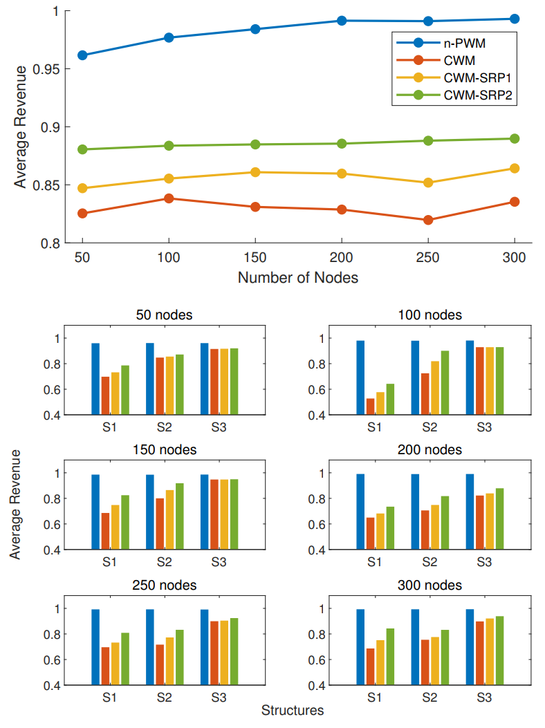
Figure 3: Results with $50\leq n\leq 300$. The above graph is the average expected revenue over all sampled structures and the following graphs give the expected revenue of some samples.

Figure 3 summarizes the results of the average revenue for different numbers of buyers. To see how the expected revenue changes in different structures, we also sampled 3 different structures for each choice of $n$ and their estimated expected revenue is shown. From the results displayed in Figure 3, we can make the following observations.

• Compared to the CWM mechanism, both the CWM-SRP mechanisms have significantly improved the expected revenue. In particular, the CWM-SRP2 always performs the best. Intuitively, with the increase in the number of buyers, the probability that buyers with high valuations are far away from the seller is higher.

• Different structures have different effects on the expected revenue, but the CWM-SRP2 always performs the best. Actually, for those structures where the CWM mechanism does not perform well, the improvement of the CWM-SRP mechanisms is more significant.

Seller Node	$n$-PWM	CWM	CWM-SRP1	CWM-SRP2
131	0.9992	0.9992	0.9992	0.9992
1323	0.9997	0.9997	0.9997	0.9997
2637	0.9995	0.9995	0.9995	0.9995
2893	0.9996	0.9996	0.9996	0.9996
3197	0.9996	0.9996	0.9996	0.9996

Table 2: Results in a Facebook network

We also conduct experiments on a real-world social network with a large number of nodes. We choose the data set ‘Social Circles: Facebook’ Leskovec and Mcauley [2012] to test the performance of these mechanisms in a real and huge network, which consists of ‘friends lists’ from the Facebook app with anonymous ids. There are 4039 nodes in total. In each experiment, we randomly choose one node as the seller and use the average revenue to approximate the expected revenue by sampling 100 groups of valuations. From the results in Table 2, we can find that all mechanisms perform well and show almost no differences. This is because the Facebook network is well-connected and most buyers can be reached by the seller without critical buyers.

Overall, we can see the CWM-SRP mechanisms can greatly improve the expected revenue, and when the graph is larger, a more aggressive shifting function may perform better. On the other hand, if the seller expects that the structure will be well-connected, simply using the CWM mechanism is sufficiently good.

References

- Bulow and Klemperer [1996] Jeremy Bulow and Paul Klemperer. Auctions versus negotiations. The American Economic Review, 86(1):180–194, 1996.
- Clarke [1971] Edward H Clarke. Multipart pricing of public goods. Public choice, pages 17–33, 1971.
- Groves [1973] Theodore Groves. Incentives in teams. Econometrica: Journal of the Econometric Society, pages 617–631, 1973.
- Guo and Hao [2021] Yuhang Guo and Dong Hao. Emerging methods of auction design in social networks. In Zhi-Hua Zhou, editor, Proceedings of the Thirtieth International Joint Conference on Artificial Intelligence, IJCAI 2021, Virtual Event / Montreal, Canada, 19-27 August 2021, pages 4434–4441. ijcai.org, 2021.
- Jeong [2020] Seungwon Eugene Jeong. The referrer’s dilemma. Available at SSRN 3514022, 2020.
- Kawasaki et al. [2020] Takehiro Kawasaki, Nathanaël Barrot, Seiji Takanashi, Taiki Todo, and Makoto Yokoo. Strategy-proof and non-wasteful multi-unit auction via social network. In The Thirty-Fourth AAAI Conference on Artificial Intelligence, pages 2062–2069, 2020.
- Lee [2016] Joosung Lee. Mechanisms with referrals: VCG mechanisms and multilevel mechanisms. In Proceedings of the 2016 ACM Conference on Economics and Computation, EC ’16, pages 789–790. ACM, 2016.
- Leskovec and Mcauley [2012] Jure Leskovec and Julian Mcauley. Learning to discover social circles in ego networks. Advances in neural information processing systems, 25, 2012.
- Li et al. [2017] Bin Li, Dong Hao, Dengji Zhao, and Tao Zhou. Mechanism design in social networks. In Proceedings of the AAAI Conference on Artificial Intelligence, volume 31, 2017.
- Li et al. [2018] Bin Li, Dong Hao, Dengji Zhao, and Tao Zhou. Customer sharing in economic networks with costs. In Proceedings of the Twenty-Seventh International Joint Conference on Artificial Intelligence, IJCAI, pages 368–374, 2018.
- Li et al. [2019] Bin Li, Dong Hao, Dengji Zhao, and Makoto Yokoo. Diffusion and auction on graphs. In Proceedings of the Twenty-Eighth International Joint Conference on Artificial Intelligence, IJCAI, pages 435–441, 2019.
- Li et al. [2020] Bin Li, Dong Hao, and Dengji Zhao. Incentive-compatible diffusion auctions. In Proceedings of the Twenty-Ninth International Joint Conference on Artificial Intelligence, IJCAI-20, pages 231–237. International Joint Conferences on Artificial Intelligence Organization, 7 2020. Main track.
- Li et al. [2022] Bin Li, Dong Hao, Hui Gao, and Dengji Zhao. Diffusion auction design. Artificial Intelligence, 303:103631, 2022.
- Myerson [1981] Roger B Myerson. Optimal auction design. Mathematics of operations research, 6(1):58–73, 1981.
- Vickrey [1961] William Vickrey. Counterspeculation, auctions, and competitive sealed tenders. The Journal of finance, 16(1):8–37, 1961.
- Watts and Strogatz [1998] Duncan J Watts and Steven H Strogatz. Collective dynamics of ‘small-world’networks. nature, 393(6684):440–442, 1998.
- Zhang et al. [2020] Wen Zhang, Dengji Zhao, and Hanyu Chen. Redistribution mechanism on networks. In Proceedings of the 19th International Conference on Autonomous Agents and Multiagent Systems, AAMAS ’20, pages 1620–1628, 2020.
- Zhao et al. [2018] Dengji Zhao, Bin Li, Junping Xu, Dong Hao, and Nicholas R. Jennings. Selling multiple items via social networks. In Proceedings of the 17th International Conference on Autonomous Agents and MultiAgent Systems, AAMAS, pages 68–76. ACM, 2018.
- Zhao [2021] Dengji Zhao. Mechanism design powered by social interactions. In Proceedings of the 20th International Conference on Autonomous Agents and MultiAgent Systems, pages 63–67, 2021.