Optimizing Energy-Harvesting Hybrid VLC/RF Networks with Random Receiver Orientation

Abstract

In this paper, we consider an indoor hybrid visible light communication (VLC) and radio frequency (RF) communication scenario with two-hop downlink transmission. The LED carries both data and energy in the first phase, VLC, to an energy harvester relay node, which then uses the harvested energy to re-transmit the decoded information to the RF user in the second phase, RF communication. The direct current (DC) bias and the assigned time duration for VLC transmission are taken into account as design parameters. The optimization problem is formulated to maximize the data rate with the assumption of decode-and-forward relaying for fixed receiver orientation. The non-convex optimization is split into two sub-problems and solved cyclically. It optimizes the data rate by solving two sub-problems: fixing time duration for VLC link to solve DC bias and fixing DC bias to solve time duration. The effect of random receiver orientation on the data rate is also studied, and closed-form expressions for both VLC and RF data rates are derived. The optimization is solved through an exhaustive search, and the results show that a higher data rate can be achieved by solving the joint problem of DC bias and time duration compared to solely optimizing the DC bias.

1 Introduction

Wireless communication services and the emergence of new technologies have created a large demand for radio frequency spectrum [2]. Visible light communications (VLC) is introduced as a promising complementary technology to radio-frequency (RF) based wireless systems, as it can be used to offload users from RF bands for releasing spectrum resources for other users while also simultaneously providing illumination [3]. Recently, hybrid VLC-RF systems have been receiving significant attention in the literature, which can be designed to take advantage of both technologies, e.g., high-speed data transmission by VLC links while achieving seamless coverage through RF links [4]. In particular, a hybrid VLC-RF system is desirable for indoor applications such as the Internet of things (IoT) or wireless sensor networks [5, 6]. Given that power constraint is a key performance bottleneck in such networks, a potential approach is to scavenge energy from the surrounding environment through energy harvesting (EH), as illustrated in Fig. 1.

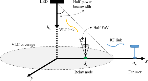
Figure 1: The system model for the considered VLC-RF transmission scenario. The VLC link carries both data and energy to the relay node. The harvested energy is then used at the relay node to forward the data to the far RF user.

The existing literature on hybrid VLC-RF systems that also use EH is mainly limited to finding the optimal value of DC bias to either maximize the data rate or minimize the outage probability [7, 8, 9, 10, 11, 12, 13, 14, 15, 16, 17, 18, 19]. To our best knowledge, optimization of VLC and RF resources for hybrid RF/VLC links for a multi-hop scenario as shown in Fig. 1 has not been studied in any works in the literature. In this paper, we investigate the performance of EH for an indoor hybrid VLC-RF scenario as shown in Fig. 1. In particular, we allocate a portion of each transmission block to VLC and the rest to RF transmission in an adaptive manner. The LED transmits both data and energy to a relay node with energy harvesting capability in the first phase as illustrated in Fig. 2 (i.e., VLC transmission). During the second phase (RF communication), the relay transmits the decoded information to the distant RF user using the harvested energy. Also, during this phase, the LED continues to transmit power (no information) to the relay node, aiming to harvest energy that can be utilized by the RF relay in the next transmission block. The key contributions of this work are summarized as follows.

• In a related study [20], a comparable policy was introduced for a single indoor link that can be based either on VLC or infrared communications (IRC) with the aim of maximizing the harvested energy; however, no RF links or relays are considered, nor is the goal to maximize the data rate. In addition, due to existence of a relay in the considered system model, its relative distance to the RF user, and its random orientation, we dynamically allocate a portion of each transmission block to VLC and the rest to RF transmission.

• For this specific scenario, we formulate an optimization problem for maximizing the data rate at the far user. In particular, different than any existing work in the literature (see e.g., [7]), we incorporate the assigned time duration to VLC link as the design parameters, in addition to the DC bias. We split the joint non-convex optimization problem over these two parameters into two sub-problems and solve them cyclically. First, we fix the assigned time duration for VLC transmission and solve the non-convex problem for DC bias by employing the majorization-minimization (MM) procedure [21] and [22]. The second step involves fixing the DC bias obtained from the previous step and solving an optimization problem for the assigned time duration of the VLC link.

• To the best of our knowledge, this is the first paper that attempts to investigate the effect of random receiver orientation for the relay on the achievable data rate for a hybrid VLC-RF network. Unlike the conventional RF wireless networks, the orientation of devices has a significant impact on VLC channel gain, especially for mobile users. Determining the exact information rate is a formidable task and may not offer valuable insights for optimizing the system’s information rate. As an alternative approach, we formulate the average information rate for the VLC link and the harvested energy based on the orientation distribution. To gain a better understanding of the influence of system and channel parameters, we assume that receiver orientation follows a uniform distribution. From this assumption, we derive a closed-form expression for the lower bound on the average information rate of both VLC and RF. To verify our analysis, we present the results for the VLC and RF information rate using three methods; i.e., exact integral expressions, simulations and the derived closed-form expressions. Based on the obtained closed-form expressions, we find the optimal values of DC bias and time allocation for the system model under consideration. Due to the complexity of the problem, an exhaustive search is conducted to solve it.

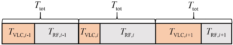
Figure 2: The transmission block under consideration with consecutive time periods dedicated for VLC (relay) and RF (access) links. The VLC link is used both as a backhaul to relay the data and for energy harvesting.

The remainder of this paper is organized as follows. Section 2 presents the literature review. In Section 3, we describe our system model. The optimization framework is introduced in Section 4, while the optimization problem and our approach to solve it are provided in Section 5. In Section 6, we derive the closed-form expressions for both VLC and RF data rate by considering random orientation, numerical results are presented in Section 7, and finally, the conclusion and future works are suggested in Section 8.

2 Literature Review

There have been some recent studies on enabling EH for a dual-hop hybrid VLC-RF communication system where the relay can harness energy from a VLC link (first hop), for re-transmitting the data to the end user over the RF link (second hop). For example, an optimal design in the sense of maximizing the data rate with respect to the direct current (DC) bias by allocating an equal time portion for VLC and RF transmission is introduced in [7]. In another work, both energy and spectral efficiency are investigated in [8] by taking into account the power consumption of the light-emitting diodes (LEDs), which clearly shows the trade-off between energy and spectral efficiency and the importance of optimizing the DC bias.

TABLE I: Summary of the most relevant works and their contributions.

Ref.	Wireless technology	Scheme	Relay power	EH during VLC trans.	EH during RF trans.	Performance metric	Optimization parameters	Random orientation
[7]	Hybrid VLC-RF	Dual-hop	Harvested energy	✓	✓	Data rate	DC bias	✗
[8]	Hybrid VLC-RF	Dual-hop	Harvested energy	✓	✗	Energy efficiency spectral efficiency	No parameter optimization	✗
[9]	Hybrid VLC-RF	Direct link	Harvested energy	✓	✗	Secrecy outage probability	No parameter optimization	✗
[10]	Hybrid VLC-RF	Cooperative	External	✗	✗	Outage probability symbol error rate	No parameter optimization	✗
[11]	Hybrid VLC-RF	Direct link	Harvested energy	✓	✗	Outage probability	No parameter optimization	✗
[12]	Hybrid VLC-RF	Dual-hop	Harvested energy	✓	✗	Outage probability	No parameter optimization	✗
[13]	Hybrid VLC-RF	Dual-hop	Harvested energy	✓	✗	Outage probability	DC bias peak amplitude	✗
[14]	Hybrid VLC-RF	Dual-hop	Harvested energy	✓	✗	Outage probability	No parameter optimization	✗
[15]	Hybrid VLC-RF	Dual-hop	Harvested energy	✓	✗	Data rate	LED transmit power UL/DL transmission time	✗
[16]	Hybrid VLC-RF	Dual-hop	Harvested energy	✓	✗	Outage probability	DC bias	✗
[17]	Hybrid VLC-RF	Cooperative	External	✗	✗	Data rate	Time duration power allocation	✗
[18]	Hybrid VLC-RF	Collaborative	N/A	✓	✓	SNR	DC bias RF beamformers	✗
[19]	Hybrid VLC-RF	Cooperative	External	✓	✗	Data rate	Access mode selection DC bias power allocation	✗
[23]	VLC only	Direct link	N/A	✗	✗	Bit error rate	No parameter optimization	✓
[24]	VLC only	Direct link	N/A	✗	✗	Outage probability	No parameter optimization	✓
[25]	VLC only	Direct link	N/A	✗	✗	Bit error rate	No parameter optimization	✓
[26]	VLC only	Direct link	N/A	✗	✗	SNR	No parameter optimization	✓
[27]	VLC only	Direct link	N/A	✗	✗	SNR	No parameter optimization	✓
This Work	Hybrid VLC-RF	Dual-hop	Harvested energy	✓	✓	Data rate	DC bias time allocation	✓

Using stochastic geometry, in [9] secrecy outage probability and the statistical characteristics of the received signal-to-noise ratio (SNR) are derived in the presence of an eavesdropper for a hybrid VLC-RF system. Outage probability and symbol error rate are studied in [10] under the assumption that the relay and destination locations are random. They consider both decode-and-forward (DF) and amplify-and-forward (AF) schemes and derive the approximated analytical and asymptotic expressions for the outage probability. In [11], the outage performance of an IoT hybrid RF/VLC system is investigated where the VLC is considered as the downlink from the LED to the IoT devices, while RF utilizes a non-orthogonal multiple access (NOMA) scheme for the uplink. Specifically, they report the approximated analytical expressions for the outage probability by utilizing a stochastic geometry approach to model the location and number of terminals in a 3-D room.

In [12], Peng et al. consider a mobile relay to facilitate the communications between the source and destination. The end-to-end outage probability of the system is analytically obtained and compared with the simulation results. They further extend this work and study the minimization problem of end-to-end outage probability under the constraints of both the average and the peak powers of the LED source in [13]. In [14], the relay is chosen among multiple IoT devices which are randomly distributed within the coverage of the source. Based on the channel state information, an analytical approach is used to determine the end-to-end outage probability for two different transmission schemes. In [15], the problem of maximizing the sum throughput of multiple users in a hybrid VLC-RF communication system were studied where the users utilize the harvested energy during downlink (DL) for transmitting in uplink (UL).

In [16], a cooperative hybrid VLC-RF relaying network has been considered and the outage probability of the VLC and RF users are calculated. Further, they derive a sub-optimal DC bias that effectively minimizes the outage probability for the RF user. More recently in [17], Rallis et al. propose a hybrid VLC-RF network where a VLC access point serves two user equipments, which also function as RF relays to expand network coverage to a third user beyond the VLC cell. Inspired by rate-splitting multiple access, the proposed protocol aims at maximizing the weighted minimum achievable rate in the system. In [18], a hybrid VLC-RF ultra-small network is introduced where the optical transmitters deliver both the lightwave information and energy signals whereas a multiple-antenna RF access point (AP) is employed to transfer wireless power over RF signals. In [19], Guo et al. consider two types of users; i.e., information users and energy-harvesting users. The information users receive information from the LED AP through time-division-multiple-access manner by either the single-hop VLC-only mode or the relay-assisted dual-hop VLC-RF mode where the relay has access to an external power source.

The existing literature on hybrid VLC-RF communication systems is mainly limited to assuming the receiver is vertically upward and fixed, and the effect of random receiver orientation on such systems has not yet been reported. The receiver orientation affects the availability of line-of-sight (LoS) links in VLC networks. In [23], Eroğlu et al. present the statistical distribution of the VLC channel gain in the presence of random orientation for mobile users. In another study [24], Fu et al. derive the average channel capacity and the outage probability based on the statistical characteristics of the channel when the VLC receivers have random locations and orientations. In [28], Rodoplu et al. study the behavior of human users and the LoS availability in an indoor environment. They further derive the outage probability and analyze the random orientation effect on inter-symbol interference. Using the Laplace distribution, Soltani et al. derive the probability density function of SNR and bit error rate for an indoor scenario [25]. There have been also some recent efforts on experimental measurements to model the receiver orientation [26, 27]. In Table I, recent studies discussing the hybrid VLC-RF communication systems and VLC receiver orientation are summarized and compared with our current work.

3 System Model

Fig. 1 illustrates the hybrid VLC-RF system under consideration. We assume a relay equipped with a single photo-detector (PD), energy-harvesting circuity, and a transmit antenna for RF communications. Let $T_{\textrm{tot}}^{(i)}$ denote the $i^{\textrm{th}}$ block transmission time which is measured in seconds. Also, $\tau_{i}$ (unitless value) is the portion of time that is allocated to transmit information and energy to the relay node in the $i^{\textrm{th}}$ time block. Thus, the duration of this phase in seconds is $T_{\textrm{VLC},{i}}=\tau_{i}T_{\textrm{tot}}^{{(i)}}$. We assume that the block transmission time is constant. Hereafter, we drop the superscript of $T_{\textrm{tot}}^{(i)}$ in the sequel to simplify notation. Fig. 2 depicts the transmission block under consideration. Without loss of generality, we assume that $T_{\textrm{tot}}=1$ second.

3.1 VLC Link

In the first hop, the LED transmits both energy and information to the relay node through the VLC link. The non-negativity of the transmitted optical signal can be assured by adding DC bias (i.e., ${I_{\textrm{b},{i}}}$) to the modulated signal, i.e., ${{x_{\textrm{t},{i}}}\left(t\right)=P_{\textrm{LED}}\big{(}{{x_{\textrm{s},{i}}}\left(t\right)+{I_{{\textrm{b}},{i}}}}\big{)}}$ where $P_{\textrm{LED}}$ denotes the LED power per unit (in W/A) and $x_{\textrm{s},{i}}$ is the modulated electrical signal. We assume that the information-bearing signal is zero-mean, and satisfies the peak-intensity constraint of the optical channel such that [20]

$$A_{{i}}\leq\min\left({{I_{\textrm{b},{i}}}-{I_{\textrm{min}}},{I_{\textrm{max}}}-{I_{\textrm{b},{i}}}}\right),$$ (1)

where $A_{{i}}$ denotes the peak amplitude of the input electrical signal (i.e., $\max(\left|{{x_{\textrm{s},{i}}}(t)}\right|)=A_{{i}}$), and ${I_{\textrm{b},{i}}}\in\left[{{I_{\textrm{min}}},{I_{\textrm{max}}}}\right]$ with ${I_{\textrm{max}}}$ and ${I_{\textrm{min}}}$ being the maximum and minimum input currents of the DC offset, respectively. Let ${B_{{\textrm{VLC}}}}$ denote the double-sided signal bandwidth.

Then, the information rate associated with the optical link between the AP and relay node within a block with $T_{\textrm{tot}}=1$ second, is given as [20]

$${R_{{\textrm{VLC}},{i}}}=T_{\textrm{VLC},{i}}{B_{{\textrm{VLC}}}}{\log_{2}}\left({1+\frac{e}{{2\pi}}\frac{{{{\left({\eta P_{\textrm{LED}}A_{{i}}{H_{\textrm{VLC}}}}\right)}^{2}}}}{{\sigma_{{\textrm{VLC}}}^{2}}}}\right),$$ (2)

where $\eta$ is the photo-detector responsivity in A/W and ${H_{{\textrm{VLC}}}}$ is the optical DC channel gain. In (2), $\sigma_{{\textrm{VLC}}}^{2}$ is the power of shot noise at the PD which is given as $\sigma_{{\textrm{VLC}}}^{2}={q_{\textrm{e}}}{I_{i}}{B_{{\textrm{VLC}}}}$ where ${q_{\textrm{e}}}$ is the charge of an electron and ${I_{i}}$ is the induced current due to the ambient light. One should note that the shot noise is the dominant noise source in the VLC channel and we ignore the thermal noise in our paper [29].The optical DC channel gain of the VLC link can be written as

$${H_{{\textrm{VLC}}}}=\frac{{\left({m+1}\right){A_{\textrm{p}}}}}{{2\pi\left({h_{\Delta}^{2}+d_{\textrm{r}}^{2}}\right)}}{\cos^{m}}\left({{\phi_{\textrm{r}}}}\right)\cos\left({{\theta_{\textrm{r}}}}\right)\Pi\left({\left|{{\theta_{\textrm{r}}}}\right|,\Phi}\right),$$ (3)

where ${h_{\Delta}}$ and ${d_{\textrm{r}}}$ are the vertical and horizontal distances, respectively, between AP and the relay node, and ${\phi_{r}}$ and ${\theta_{r}}$ are the respective angle of irradiance and incidence, respectively. The Lambertian order is $m={{-1}\mathord{\left/{\vphantom{{-1}{{{\log}_{2}}\left({\cos\left(\Theta\right)}\right)}}}\right.\kern-1.2pt}{{{\log}_{2}}\left({\cos\left(\Theta\right)}\right)}}$ where $\Theta$ is the half-power beamwidth of each LED, and ${A_{\textrm{p}}}$ and $\Phi$ are the detection area and half field-of-view (FoV) of the PD, respectively. The function $\Pi\left({x,y}\right)$ is 1 whenever $x\leq y$, and is 0 otherwise. We also assume that the relay node distance follows a Uniform distribution with $\mathcal{U}\left[{d_{\textrm{r},{\min}},d_{\textrm{r},{\max}}}\right]$, and that relay PD is looking directly upward.

The harvested energy at this phase can be computed as [20]

$${E_{\textrm{1},{i}}}=0.75T_{\textrm{VLC},{i}}{I_{{\textrm{DC}},{i}}}{V_{\textrm{t}}}\ln\left({1+\frac{I_{{\textrm{DC}},{i}}}{{{I_{0}}}}}\right),$$ (4)

where ${V_{\textrm{t}}}$ is the thermal voltage, ${I_{0}}$ is the dark saturation current, and ${I_{{\textrm{DC}},{i}}}$ is the DC part of the output current given as $I_{{\textrm{DC}},{i}}=\eta{H_{{\textrm{VLC}}}}P_{\textrm{LED}}{I_{\textrm{b},{i}}}$. In the time period $T_{\textrm{RF},{i}}=1-T_{\textrm{VLC},{i}}$, the aim is to maximize the harvested energy while the relay transmits the information to the far user over the RF link. Thus, during the second phase, the LED eliminates the alternating current (AC) part and maximizes the DC bias, i.e., $A_{{i}}=0$ and $I_{\textrm{b},{i}}=I_{\textrm{max}}$. Mathematically speaking, the harvested energy during the second phase can be expressed as

$${E_{2,{i}}}=0.75T_{\textrm{RF},{i}}{I_{\textrm{DC, max}}}{V_{\textrm{t}}}\ln\!\left(\!{1+\frac{I_{\textrm{DC, max}}}{I_{0}}}\!\right),$$ (5)

where $I_{\textrm{DC, max}}=\eta{H_{{\textrm{VLC}}}}P_{\textrm{LED}}{I_{\textrm{max}}}$.

The total harvested energy at the relay that can be utilized for transmitting the decoded symbol to the far user through an RF link can be calculated as

$$\begin{split}E_{\textrm{h},{i}}=&{E_{1,{i}}}+{E_{2,{i-1}}}\\ =&z\bigg{(}T_{\textrm{VLC},{i}}I_{\textrm{b},{i}}\ln{\Big{(}1+\frac{\eta H_{\textrm{VLC}}P_{\textrm{LED}}I_{\textrm{b},{i}}}{I_{0}}\Big{)}}\\ &+T_{\textrm{RF},{i-1}}I_{\textrm{max}}\ln{\Big{(}1+\frac{\eta H_{\textrm{VLC}}P_{\textrm{LED}}I_{\textrm{max}}}{I_{0}}\Big{)}}\bigg{)},\end{split}$$ (6)

where $z=0.75\eta H_{\textrm{VLC}}P_{\textrm{LED}}V_{\textrm{t}}$, ${E_{2,{i}}}$ represents the harvested energy during the RF transmission in the previous transmission block. In this paper, we assume that the initial harvested energy is 0 (i.e., ${E_{2,0}}=0$).

As it can be readily checked from (1), increasing $I_{\textrm{b},i}$ leads to a decrease in $A_{i}$ and, consequently, it decreases the information rate associated with the VLC link. On the other hand, decreasing $I_{\textrm{b},i}$ limits the harvested energy that can be obtained during VLC transmission (i.e., $E_{\textrm{1},{i}}$).

3.2 RF Link

In the second hop, the relay re-transmits the information to the far user through the RF link by utilizing the harvested energy. We assume that the energy used for data reception at the relay is practically negligible and the harvested energy is primarily employed for data transmission [7, 16]. The relaying operation is of DF type. We assumed that the user is away from the AP horizontally by a distance ${d_{\textrm{u}}}$, which follows a Uniform distribution with $\mathcal{U}\left[{d_{\textrm{u, min}},d_{\textrm{u, max}}}\right]$. Let ${B_{{\textrm{RF}}}}$ denote the bandwidth for the RF system and ${N_{0}}$ denote the noise power which can be defined as ${{N_{0}}={P_{0}}+10{\log_{10}}\left({{B_{{\textrm{RF}}}}}\right)+{N_{\textrm{F}}}}$ where ${P_{0}}$ is the thermal noise power, and ${N_{\textrm{F}}}$ is the noise figure. Further, assume that the relay re-transmits the electrical signal with normalized power. The respective information rate is given as

$${R_{\textrm{RF},{i}}}=T_{\textrm{RF},{i}}{B_{{\textrm{RF}}}}{\log_{2}}\left({1+\frac{{{{P_{\textrm{h},{i}}}}{{\left|{{h_{{\textrm{RF}}}}}\right|}^{2}}}}{{{G_{{\textrm{RF}}}}{N_{0}}}}}\right),$$ (7)

where ${h_{{\textrm{RF}}}}$ denotes the Rayleigh channel coefficients, ${{P_{\textrm{h},{i}}}={E_{\textrm{h},{i}}}/T_{\textrm{RF},{i}}}$ is the transmit power and ${G_{{\textrm{RF}}}}$ is the path loss model for RF link and can be expressed as

$${G_{{\textrm{RF}}}}={\left({\frac{{4\pi{d_{0}}}}{\lambda}}\right)^{2}}{\left({\frac{d_{\textrm{u}}}{{{d_{0}}}}}\right)^{\beta}},$$ (8)

where $\lambda$ is the used RF carrier wavelength, ${d_{0}}=1$ m is the reference distance, and $\beta$ is the path loss exponent, which generally takes a value between [1.6, 1.8] [30].

The achievable information rate is limited by the smaller information rate between the VLC link and the RF link and can be expressed as [19]

$$R_{\textrm{VLC-RF},{i}}=\min{(R_{\textrm{VLC},{i}},R_{\textrm{RF},{i}})}.$$ (9)

Fig. 3 illustrates the effect of time allocation and DC bias on information data rate. Unless otherwise stated, the system and channel parameters can be found in Table II. We assume the relay is located at $d_{\textrm{r}}=0$ m, the user is at $d_{\textrm{u}}=4$ m, and the RF frequency sets as $f_{\textrm{c}}=2.4$ GHz. Fig. 3(a) illustrates the information data rate for the VLC and RF links versus the time allocation of the VLC link. In this figure, we assume DC bias as $I_{\textrm{b}}\in\{0.6,0.8\}$ A. Since we assume that the block transmission time is constant ($T_{\textrm{VLC},i}+T_{\textrm{RF},i}=1$), as the VLC time portion increases the RF time portion decreases. As it can be observed from Fig. 3(a), increasing the time allocation for the VLC link (i.e., $T_{\textrm{VLC}}$) results in increasing the VLC data rate while it decreases the harvested energy during the second phase (see (5)) and consequently decreases the RF data rate. Fig. 3(b) depicts the information rate for VLC and RF link versus DC bias. Here, we assume an equal time portion for VLC and RF transmission (i.e., $T_{\textrm{VLC}}=T_{\textrm{RF}}=0.5$) as well as $T_{\textrm{VLC}}=0.8$ (consequently $T_{\textrm{RF}}=0.2$). Recalling (1), we can observe that increasing DC bias leads to a reduction in peak amplitude of the input electrical signal (i.e., $A_{i}$) and subsequently VLC data rate. However, as DC bias increases the harvested energy in the first phase (see (4)) increases which eventually results in a higher RF data rate.

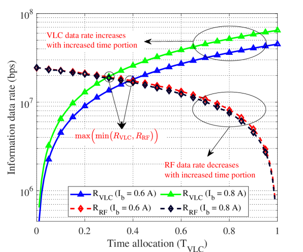
(a) Fixed $I_{\textrm{b}}$.

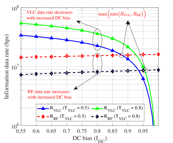
(b) Fixed $T_{\textrm{VLC}}$.

Figure 3: The VLC and RF information rate when $d_{\textrm{r}}=0$ m, $d_{\textrm{u}}=4$ m, and $f_{\textrm{c}}=2.4$ GHz for (a) fixed DC bias and (b) equal time allocation.

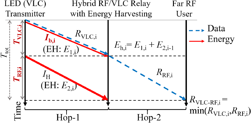
Figure 4: Summary of the optimization problem. Here, we consider $I_{\textrm{b},i}$, $T_{\textrm{VLC},i}$, and $T_{\textrm{RF},i}$ as the optimization variables to maximize the system data rate.

4 Optimization Framework

Our aim is to optimize the achievable information rate (i.e., (9)) over $I_{\textrm{b},i}$ and $T_{\textrm{VLC},i}$. Fig. 4 summarizes the optimization problem of maximizing the system data rate, with the optimization variables represented in red. Recalling the information rate in VLC link (i.e., (2)) and RF link (i.e., (7)), the optimization problem can be written as

$$\max_{I_{\textrm{b},{i}},T_{\textrm{VLC},{i}},T_{\textrm{RF},{i}}} R_{\textrm{VLC-RF},{i}}$$ (10)

s.t. $$c_{1}:I_{\textrm{min}}\leq I_{\textrm{b},{i}}\leq I_{\textrm{max}},$$

$$c_{2}:T_{\textrm{VLC},{i}}\!+\!T_{\textrm{RF},{i}}\!=\!1,T_{\textrm{VLC},{i}}>0,T_{\textrm{RF},{i}}>0$$

$$c_{3}:R_{\textrm{th}}\leq R_{\textrm{RF}}^{i}.$$

where $R_{\textrm{th}}$ is a predefined threshold value, and constraint $c_{1}$ is imposed to avoid any clipping and guarantee that the LED operates in its linear region. Since the relay re-transmits the information and the RF far user is unable to receive data from the LED, $c_{3}$ is added to satisfy the minimum required data rate.

The joint-optimization problem in (10) is non-smooth (due to the $\min$ operator) and non-convex (due to the objective function and constraint $c_{3}$). We reformulate the above optimization problem in the epigraph form to remove the non-smoothness in the objective function. Referring to [31, Chapter 4], the epigraph form of (10) can be written as

$$\max_{\phi,I_{\textrm{b},{i}},T_{\textrm{VLC},{i}},T_{\textrm{RF},{i}}}\quad\phi$$ (11)

s.t. $$c_{1},c_{2},c_{3},$$

$$c_{4}:\phi\leq R_{\textrm{VLC},{i}}$$

$$c_{5}:\phi\leq R_{\textrm{RF},{i}}.$$

The above equivalent optimization problem to (10) solves the non-smoothness, while it is still non-convex. Let ${\alpha={e\left({\eta P_{\textrm{LED}}{H_{\textrm{VLC}}}}\right)}^{2}/(2\pi\sigma_{{\textrm{VLC}}}^{2})}$, ${\beta=\eta{H_{{\textrm{VLC}}}}P_{\textrm{LED}}}$, and ${\zeta=|h_{\textrm{RF}}|^{2}/(G_{\textrm{RF}}N_{0})}$. Substituting (2) and (7) in (11), we have

$$\max_{\phi,I_{\textrm{b},{i}},A_{i},E_{\textrm{h},{i}},T_{\textrm{VLC},{i}},T_{\textrm{RF},{i}}}\ \phi$$ (12)

s.t. $$c_{1}^{\prime},c_{2},$$

$$c_{3}:T_{\textrm{RF},{i}}B_{\textrm{RF}}\!\log_{2}\!\!\left(\!\!1\!+\!\frac{\zeta E_{\textrm{h},{i}}}{T_{\textrm{RF},{i}}}\!\right)\!\!\geq\!\!R_{\textrm{th}},$$

$$c_{4}:T_{\textrm{VLC},{i}}B_{\textrm{VLC}}\log_{2}(1+\alpha A_{i}^{2})\!\!\geq\!\phi,$$

$$c_{5}:T_{\textrm{RF},{i}}B_{\textrm{RF}}\log_{2}\!\left(\!1\!+\!\frac{\zeta E_{\textrm{h},{i}}}{T_{\textrm{RF},{i}}}\right)\!\geq\!\phi,$$

$$c_{6}:\min\big{(}I_{\textrm{b},{i}}-I_{\textrm{min}},I_{\textrm{max}}-I_{\textrm{b},{i}}\big{)}\!\geq\!A_{i},$$

$$c_{7}:z\Big{(}T_{\textrm{VLC},{i}}I_{\textrm{b},{i}}\ln{\big{(}1+\frac{\beta I_{\textrm{b},{i}}}{I_{0}}\big{)}}$$

$$\quad+\!T_{\textrm{RF},{i-1}}I_{\textrm{max}}\!\ln\!{\big{(}1\!+\!\frac{\beta I_{\textrm{max}}}{I_{0}}\big{)}}\!\Big{)}\!\!\geq\!E_{\textrm{h},{i}}.$$

In the optimization problem of (12), $A_{i}^{2}$ is used in $c_{4}$ and $c_{6}$ is still non-smooth. Here, we relax $c_{6}$ by using Proposition 1 from [19]. Intuitively, as $I_{\textrm{b,i}}$ increases the harvested energy increases; however, it has a negative effect on the rate beyond $(I_{\textrm{min}}+I_{\textrm{max}})/2$. Thus, the optimal value of the term $I_{\textrm{b,i}}$ would be within $(I_{\textrm{min}}+I_{\textrm{max}})/2$ and $I_{\textrm{max}}$ (and not the other regime ${0\leq I_{\textrm{b, i}}\leq I_{\textrm{max}})}$. The above restriction enforces $0\leq A_{i}\leq I_{\textrm{max}}-I_{\textrm{b},{i}}$ benefiting in getting rid of the non-smooth $\min$ operator (see (12)) as well. This leads to ${c_{1}^{\prime}:(I_{\textrm{min}}+I_{\textrm{max}})/{2}\leq I_{\textrm{b},i}\leq I_{\textrm{max}}}$ and $c_{6}^{\prime}:0\leq A_{i}\leq I_{\textrm{max}}-I_{\textrm{b},{i}}$. The constraints $c_{3},c_{4},c_{5}$, and $c_{7}$ are jointly non-convex. In this regard, we split the joint optimization problem into two sub-problems and solve them in a cyclic fashion which will be elaborated in the next section.

5 Solution Approach

In this section, we consider two sub-problems for solving (12). In sub-problem 1, we solve the maximization problem for $\phi$ over $I_{\textrm{b},{i}},A_{i},E_{\textrm{h},{i}}$ by fixing the time allocation $T_{\textrm{VLC},{i}}$. In the second sub-problem, we solve the maximization problem for $\phi$ over $T_{\textrm{VLC},{i}},T_{\textrm{RF},{i}},E_{\textrm{h},{i}}$ by using $I_{\textrm{b},{i}}$ obtained from sub-problem 1.

5.1 Sub-problem 1

First, we fix $T_{\textrm{VLC},{i}}$ (and hence $T_{\textrm{RF},{i}}=1-T_{\textrm{VLC},{i}}$) and solve the maximization problem for $\phi$ over $I_{\textrm{b},{i}},A_{i},E_{\textrm{h},{i}}$. Sub-problem 1 can be written as

$$\max_{\phi,I_{\textrm{b},{i}},A_{i},E_{\textrm{h},{i}}} \phi$$ (13)

s.t. $$c_{1}^{\prime},c_{3},c_{4},c_{5},c_{7}$$

$$c_{6}^{\prime}:0\leq A_{i}\leq I_{\textrm{max}}-I_{\textrm{b},{i}},$$

where the constraints $c_{3},c_{4},c_{5}$ are conditionally convex.

Assumption: The typical illumination requirement in an indoor VLC environment results in a high transmit optical intensity, which can provide a high SNR at the receiver [32, 33]. In this paper, we assume that SNR for the VLC link is much greater than 1 (in linear scale); i.e., $\alpha(A_{i})^{2}\gg 1$. In this condition, we further utilize ${\log(1+x)\approx\log(x)}$ in the constraints $c_{4}$. Thus, the optimization problem can be written as

$$\max_{\phi,I_{\textrm{b},{i}},A_{i},E_{\textrm{h},{i}}} \phi$$ (14)

s.t. $$c_{1}^{\prime},c_{3},c_{5},c_{6}^{\prime}$$

$$c_{4}^{\prime}:T_{\textrm{VLC},{i}}B_{\textrm{VLC}}\log_{2}(\alpha A_{i}^{2})\geq\phi,$$

$$c_{7}^{\prime}:z\bigg{(}T_{\textrm{VLC},{i}}I_{\textrm{b},{i}}\ln{\Big{(}\frac{\beta I_{\textrm{b},{i}}}{I_{0}}\Big{)}}$$

$$\quad+\!T_{\textrm{RF},{i-1}}I_{\textrm{max}}\ln\!{\Big{(}\!\frac{\beta I_{\textrm{max}}}{I_{0}}\Big{)}}\bigg{)}\!\geq\!E_{\textrm{h},{i}}.$$

In (14), $c_{4}^{\prime}$ is a convex constraint while $c_{7}^{\prime}$ is still not convex. We further utilize the first-order Taylor series and MM approach to relax this constraint [21, 22]. As a result, $c_{7}^{\prime}$ can be replaced with

$$c_{7}^{\star}:\quad g(I_{\textrm{b},{i}})=g_{0}\big{(}I_{\textrm{b},{i}}(t)\big{)}+\frac{\partial g\big{(}I_{\textrm{b},{i}}(t)\big{)}}{\partial I_{\textrm{b},{i}}}\big{(}I_{\textrm{b},{i}}-I_{\textrm{b},{i}}(t)\big{)},$$ (15)

where

$$g_{0}(I_{\textrm{b},{i}}(t))= z\bigg{(}T_{\textrm{VLC},{i}}I_{\textrm{b},{i}}(t)\ln{\Big{(}\frac{\beta I_{\textrm{b},{i}}(t)}{I_{0}}\Big{)}}$$ (16)

$$+T_{\textrm{RF},{i}-1}I_{\textrm{max}}\ln{\Big{(}\frac{\beta I_{\textrm{max}}}{I_{0}}\Big{)}}\bigg{)},$$

and

$$\frac{\partial g(I_{\textrm{b},{i}}(t))}{\partial I_{\textrm{b},{i}}} =zT_{\textrm{VLC},{i}}\bigg{(}\ln{\Big{(}\frac{\beta I_{\textrm{b},{i}}(t)}{I_{0}}\Big{)}}+\frac{\beta I_{\textrm{b},{i}}(t)}{I_{0}+\beta I_{\textrm{b},{i}}(t)}\bigg{)}.$$ (17)

In (15), the term $t$ is an index-term and denotes the iteration index for the MM approach. The MM procedure on (15) operates iteratively. We first solve the problem for some initial values of $I_{\textrm{b},{i}}(t)$. Then, we update the value of $I_{\textrm{b},{i}}(t)$ at each iteration until it remains the same for two consecutive iterations, or the change between two consecutive iterations is not appreciable.

Overall, the optimization sub-problem 1 is as follows:

$$\max_{\phi,I_{\textrm{b},{i}},A_{i},E_{\textrm{h},{i}}}\quad\phi$$ (18)

s.t. $$c_{1},c_{3},c_{4}^{\prime},c_{5},c_{6}^{\prime},c_{7}^{\star}.$$

We iteratively solve the above sub-problem 1 until its convergence. Once the above sub-problem converges, we continue with sub-problem 2 which is elaborated in the following.

5.2 Sub-problem 2

In here, we fix $I_{\textrm{b},{i}}$ obtained from sub-problem 1 and solve the problem for maximizing $\phi$ over the variables $T_{\textrm{VLC},{i}},T_{\textrm{RF},{i}},E_{\textrm{h},{i}}$. The optimization problem can be expressed as

$$\max_{\phi,T_{\textrm{VLC},{i}},T_{\textrm{RF},{i}},E_{\textrm{h},{i}}}\quad\phi$$ (19)

s.t. $$c_{2},c_{3},c_{4}^{\prime},c_{5},c_{7}^{\prime}.$$

In (19), the objective function and constraints $c_{2},c_{4}^{\prime},c_{7}^{\prime}$ are linear, whereas the constraints $c_{3}$ and $c_{5}$ are convex constraints which result in a convex optimization problem.

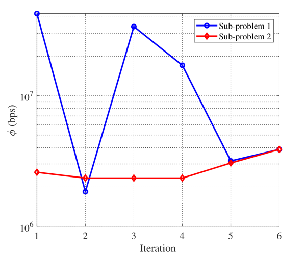
Figure 5: The performance of our optimization framework when $d_{r}=0$ m and $d_{u}=4$ m.

5.3 Convergence

Here, we study the convergence of our proposed optimization algorithm. We assume that the relay location is at $d_{r}=0$ m while the far user distance is $d_{u}=4$ m. As it can be observed from Fig. 5, the achievable information rate obtained for sub-problem 1 is higher than the one obtained for sub-problem 2.However, after five iterations, rates obtained in the two sub-problems converge and the difference between the information rate of the sub-problems becomes negligible.

6 Relay Random Orientation

In this section, we investigate the effect of relay random orientation on the achievable data rate for the considered scenario in Figs. 1, 2, and 4. Random orientation can significantly influence channel quality. This effect not only degrades the VLC data rate but also influences the RF data rate since the relay is empowered by the harvested energy. Here, we assume wide FOV where the incidence angle $\theta_{\textrm{r}}$ in (3) is always smaller than $\Theta$ which implies $\Pi\left({\left|\theta_{\textrm{r}}\right|,\Phi}\right)=1$; therefore the LED is always within the FOV. To separate the deterministic and random parts, we can rearrange (3) as follows:

$$H_{{\textrm{VLC}}}=\frac{{\left({m+1}\right){A_{\textrm{p}}}{h_{\Delta}^{m}}}}{{2\pi}}{\left({{h_{\Delta}^{2}}+{d_{\textrm{r}}^{2}}}\right)^{-\frac{{m+2}}{2}}}\cos\left(\theta_{\textrm{r}}\right),$$ (20)

where we employ the geometrical relation

$$\cos\left({{\phi}_{\textrm{r}}}\right)=\frac{h_{\Delta}}{\sqrt{d_{\textrm{r}}^{2}+{h_{\Delta}^{2}}}}.$$

Let $H_{\textrm{VLC}}=h_{\textrm{c}}h_{\theta}$ where

$${h_{\textrm{c}}=\frac{{\left({m+1}\right){A_{\textrm{p}}}{h_{\Delta}^{m}}}}{{2\pi}}{\left({{h_{\Delta}^{2}}+{d_{\textrm{r}}^{2}}}\right)^{-\frac{{m+2}}{2}}}}$$

is the deterministic part of (20) and $h_{\theta}=\cos(\theta_{\textrm{r}})$. The distribution of the square channel can be derived by considering the probability density function (PDF) of $h_{\theta}^{2}=\cos^{2}(\theta_{\textrm{r}})$ given as [23]

$${f_{h_{\theta}^{2}}}\left(x\right)=\frac{{{c_{\theta}}}}{{\sqrt{4x\left({1-x}\right)}}}{f_{\theta}}\left({\frac{1}{2}{{\cos}^{-1}}\left({2x-1}\right)}\right),$$ (21)

for $0\leq x\leq 1$, and 0 otherwise. In (21), $c_{\theta}$ is the normalization constant and $f_{\theta}(\cdot)$ is the PDF of the random angle $\theta$. As a result, the PDF of the square channel is readily given as [23]

$$f_{h^{2}}(x)=\frac{1}{h_{c}^{2}}{f_{h_{\theta}^{2}}}\Big{(}\frac{x}{h_{c}^{2}}\Big{)}.$$ (22)

6.1 Average VLC data rate

In this condition, the average data rate for the VLC link can be calculated as

$$\begin{split}{R_{{\textrm{VLC}},{i}}}^{\textrm{avg}}=&\int T_{\textrm{VLC},{i}}{B_{{\textrm{VLC}}}}\\ &\times{\log_{2}}\left({1+\frac{e}{{2\pi}}\frac{{{{\left({\eta P_{\textrm{LED}}A_{{i}}}\right)}^{2}}}}{{\sigma_{{\textrm{VLC}}}^{2}}}}x\right)f_{h^{2}}(x)\text{{d}}x,\end{split}$$ (23)

It is worth mentioning that $f_{\textrm{h}^{2}}$ is 0 for $x<0$ and $x>h_{\textrm{c}}^{2}$. In this paper, we assume $\theta$ follows $\theta\sim U[\theta_{1},\theta_{2}]$. As a result, We can rewrite (22) as

$$f_{h^{2}}(x)=\frac{{c_{\theta}}}{(\theta_{2}-\theta_{1}){\sqrt{4x\left({1-x}\right)}}}.$$ (24)

Inserting (24) into (23), and substituting $t\coloneqq x/h_{\textrm{c}}^{2}$ we have

$${R_{{\textrm{VLC}},{i}}}^{\textrm{avg}}=L_{1}\int\frac{{\log_{2}}{\left({1+L_{2}}t\right)}}{{\sqrt{4t\left({1-t}\right)}}}\text{{d}}t,$$ (25)

where $L_{1}=\frac{{c_{\theta}}T_{\textrm{VLC},{i}}{B_{{\textrm{VLC}}}}}{\theta_{2}-\theta_{1}}$ and $L_{2}=\frac{e}{{2\pi}}\frac{{{{\left({\eta P_{\textrm{LED}}A_{{i}}}{h_{\textrm{c}}}\right)}^{2}}}}{{\sigma_{{\textrm{VLC}}}^{2}}}$. Utilizing the first two terms of Puiseux series[34] $x=1$ for ${1\mathord{\left/{\vphantom{1{\sqrt{4x(1-x)}}}}\right.\kern-1.2pt}{\sqrt{4x(1-x)}}}$, a lower bound on (25) can be written as

$$\begin{split}{R_{{\textrm{VLC}},{i}}}^{\textrm{avg}}\!\geq\!L_{1}\!\Bigg{(}\!\!\int\!\!\frac{{\log_{2}}{\left({1\!+\!L_{2}}t\right)}}{2{\sqrt{\left({1-t}\right)}}}\text{{d}}t\!\!+\!\!\int\!\!\frac{\sqrt{1-t}{\log_{2}}\left({1\!+\!L_{2}}t\right)}{4}\text{{d}}t\!\!\Bigg{)}.\end{split}$$ (26)

Using 2.727.5 of [35], the first integral term of (26) can be written as

$$\begin{split}f_{1}(x,L_{2})&=\int\frac{{\log_{2}}\left({1+L_{2}}t\right)}{2{\sqrt{\left({1-t}\right)}}}\text{{d}}t\\ &=\frac{-1}{\sqrt{L_{2}}}\bigg{(}\left(\ln(x)-2\right)\sqrt{L_{2}+1-x}\\ &-2\sqrt{L_{2}+1}\ln{\frac{\sqrt{L_{2}+1-x}-\sqrt{L_{2}+1}}{\sqrt{x}}}\bigg{)}.\end{split}$$ (27)

Using an integral solver [36], the second integral in (26) can be written as

$$\begin{split}&f_{2}(x,L_{2})=\int\frac{\sqrt{1-t}{\log_{2}}\left({1+L_{2}}t\right)}{4}\text{{d}}t\\ &=\frac{1}{4}\!\Bigg{(}\!\frac{2\sqrt{1\!-\!x}(-2L_{2}(x\!-\!4)\!\!+\!\!3L_{2}(x\!-\!1)\ln{(L_{2}x\!+\!1\!)}\!\!+\!\!6)}{9L_{2}}\\ &-\frac{4}{3}\left(\frac{L_{2}+1}{L_{2}}\right)^{(3/2)}{\tanh}^{-1}{\bigg{(}\sqrt{\frac{L_{2}(1-x)}{L_{2}+1}}\bigg{)}}\Bigg{)}.\end{split}$$ (28)

The final result for (26) can then be expressed as

$$\begin{split}{R_{{\textrm{VLC}},{i}}}^{\textrm{avg}}&\geq L_{1}\\ &\times\bigg{(}f_{1}({\frac{\cos{(2\theta_{1})}+1}{2}},L_{2})+f_{2}(\!{\frac{\cos{(2\theta_{1})}+1}{2}},L_{2}\!)\\ &-f_{1}({\frac{\cos{(2\theta_{2})}+1}{2}},L_{2})-f_{2}({\frac{\cos{(2\theta_{2})}+1}{2}},L_{2})\bigg{)}.\end{split}$$ (29)

6.2 Average Energy Harvesting

Recalling (6) and utilizing $\ln{(1+x)}\approx\ln{(x)}$, the total harvesting energy can be written as

$$\begin{split}\tilde{E}_{\textrm{h},{i}}\approx M_{1}H_{\textrm{VLC}}\ln{(M_{2}H_{\textrm{VLC}})}+M_{3}H_{\textrm{VLC}}\ln{(M_{4}H_{\textrm{VLC}})}\end{split}$$ (30)

where

$$M_{1}=0.75T_{\textrm{VLC}}\eta P_{\textrm{LED}}I_{\textrm{b, i}}V_{\textrm{t}},$$ (31)

$$M_{2}=\eta P_{\textrm{LED}}I_{\textrm{b, i}}/I_{0},$$ (32)

$$M_{3}=0.75T_{\textrm{RF}}\eta P_{\textrm{LED}}I_{\textrm{max}}V_{\textrm{t}},$$ (33)

and

$$M_{4}=\eta P_{\textrm{LED}}I_{\textrm{max}}/I_{0}.$$ (34)

The PDF of $h_{\theta}$ can be expressed as

$$f_{h_{\theta}}(x)=1/(\theta_{2}-\theta_{1})\sqrt{(1-\cos^{-1}(x))}$$ (35)

for ${\cos{\theta_{1}}\leq x\leq\cos{\theta_{2}}}$. As a result, the PDF of VLC channel can be calculated as $f_{h}(x)=\frac{1}{h_{c}}f_{h_{\theta}}(\frac{x}{h_{c}})$. The average energy harvesting can be calculated as

$$\begin{split}\bar{E}_{\textrm{h},{i}}=&\int_{0}^{\infty}(M_{1}x\ln{(M_{2}x})+M_{3}x\ln{(M_{4}x)})f_{h}(x)\text{{d}}x\end{split}$$ (36)

Utilizing $\ln{(ab)}=\ln{(a)}+\ln{(b)}$ and defining $f_{3}(x)$ and $f_{4}(x)$ as

$$\begin{split}f_{3}(x)=&\int_{h_{c}\cos{\theta_{2}}}^{h_{c}\cos{\theta_{1}}}\frac{x}{\sqrt{1-\frac{x}{h_{c}}}}\text{{d}}x\\ =&-h_{c}\sqrt{h_{c}^{2}-x^{2}}\end{split}$$ (37)

and

$$\begin{split}&f_{4}(x)=\int_{h_{c}\cos{\theta_{2}}}^{h_{c}\cos{\theta_{1}}}\frac{x\ln{x}}{\sqrt{1-\frac{x}{h_{c}}}}\text{{d}}x\\ =&\!-\!h_{c}\Big{(}h_{c}\tanh^{-1}\big{(}\!\frac{\sqrt{h_{c}^{2}\!-\!x^{2}}}{h_{c}}\!\big{)}\!\!+\!\!\sqrt{h_{c}^{2}-x^{2}}\big{(}\ln{(x)}\!-\!1\big{)}\Big{)}.\end{split}$$ (38)

Thus, the final expression for (36) can be written as

$$\begin{split}\bar{E}_{\textrm{h},{i}}=&\frac{M_{1}}{h_{c}(\theta_{2}-\theta_{1})}\bigg{(}\ln{(M_{2})}f_{3}(h_{c}\cos{\theta_{1}})+f_{4}(h_{c}\cos{\theta_{1}})\\ &-\ln{(M_{2})}f_{3}(h_{c}\cos{\theta_{2}})-f_{4}(h_{c}\cos{\theta_{2}})\bigg{)}\\ +&\frac{M_{3}}{h_{c}(\theta_{2}-\theta_{1})}\bigg{(}\ln{(M_{4})}f_{3}(h_{c}\cos{\theta_{1}})+f_{4}(h_{c}\cos{\theta_{1}})\\ &-\ln{(M_{4})}f_{3}(h_{c}\cos{\theta_{2}})-f_{4}(h_{c}\cos{\theta_{2}})\bigg{)}.\end{split}$$ (39)

Therefore, a lower bound on the average data rate for RF link can be calculated as

$${R_{\textrm{RF},{i}}}^{\textrm{avg}}\geq T_{\textrm{RF},{i}}{B_{{\textrm{RF}}}}{\log_{2}}\left({1+\frac{\bar{E}_{\textrm{h},i}{{{\left|{{h_{{\textrm{RF}}}}}\right|}^{2}}}}{T_{\textrm{RF},i}{{G_{{\textrm{RF}}}}{N_{0}}}}}\right).$$ (40)

TABLE II: System and channel parameters that are used to generate the numerical results.

Parameter	Numerical Value
User distance ($d_{\textrm{u},{\textrm{min}}}$,$d_{\textrm{u},{\textrm{max}}}$)	[4,8] m
Relay distance ($d_{\textrm{r},{\textrm{min}}}$,$d_{\textrm{r},{\textrm{max}}}$)	[0,2] m
LED power ($P_{\textrm{LED}}$)	1.5 W/A
Noise figure ($N_{\textrm{F}}$)	9 dB  [8]
RF signal bandwidth $B_{\textrm{RF}}$	10 MHz [19]
VLC signal bandwidth $B_{\textrm{VLC}}$	10 MHz [19]
Thermal noise ($P_{0}$)	-174 dBm/Hz [8]
RF frequency ($f_{\textrm{c}}$)	{2.4, 5} GHz [8]
Minimum DC bias ($I_{\textrm{min}}$)	100 mA  [8]
Maximum DC bias ($I_{\textrm{max}}$)	1 A  [8]
Photo-detector responsivity ($\eta$ )	0.4 A/W [20]
Thermal voltage ($V_{\textrm{t}}$)	25 mV [8]
Dark saturation current ($I_{0}$)	$10^{-10}$ A [8]
Half FoV ($\Phi$)	$60^{\circ}$ [8]
Half-power beamwidth ($\Theta$)	$60^{\circ}$ [8]
Electron charge ($q_{\textrm{e}}$)	$1.6\times 10^{-19}$
Induced current ($I_{i}$)	$5840\times 10^{-6}$ [8]
PD detection area ($A_{\textrm{p}}$)	$10^{-4}$ $\textrm{m}^{2}$ [8]
AP relative height ($h_{\Delta}$)	2 m [8]
Data rate threshold ($R_{\textrm{th}}$)	$10^{6}$ b/s

7 Numerical Results

In this section, we demonstrate the performance of hybrid VLC-RF scheme under consideration as in Fig. 1 using computer simulations. For the convenience of the reader, unless otherwise stated, the channel and system parameters are summarized in Table II.

7.1 Approximation and Closed-form Expressions

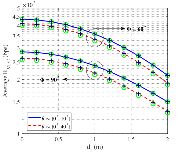
Figure 6: The performance of VLC data rate through the exact expression (i.e., (23)), simulation as illustrated with a black plus sign marker (+) and the closed-form (i.e., (29)) as illustrated with a green circle marker (o) versus the horizontal distance between the relay and the VLC AP.

(a) $\Phi=60^{\circ}$.

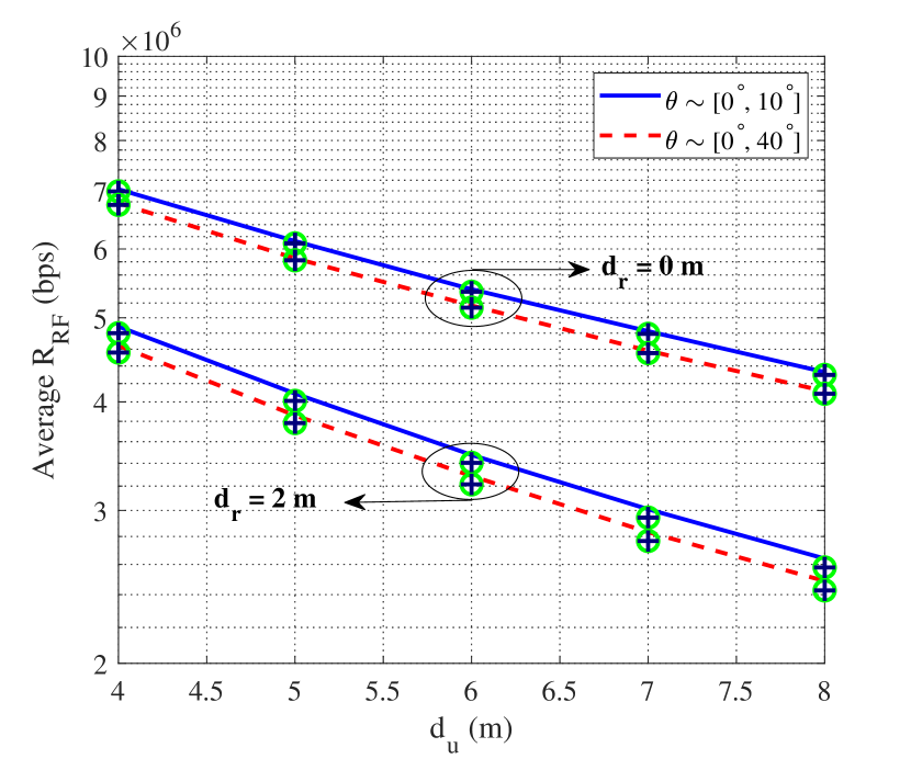
(b) $\Phi=90^{\circ}$.

Figure 7: The performance of RF data rate obtained using computer simulations, using (36) as illustrated with circle marker and using the closed-form expression (i.e., (39)) as illustrated with plus sign marker.

In this subsection, we first compare the performance of VLC with random receiver orientation data rate using the exact expression in (23), simulation, and the closed-form approximation in (29). We assume the relay location varies as $d_{\textrm{r}}\in\{0,2\}$ and the half-power beamwidth as $\Phi\in\{60^{\circ},90^{\circ}\}$. To verify our expressions, we consider two case; $\theta\sim U[0^{\circ},10^{\circ}]$ and $\theta\sim U[10^{\circ},40^{\circ}]$. We assume $A_{i}=0.2$, $T_{\textrm{VLC, i}}=0.8$. Fig. 6 depicts the effect of random orientation on the average of VLC data rate. As it can be observed from Fig. 6, the simulation results and the exact expression are completely matched and there is a practically negligible mismatch for the closed-form expression. As can be readily checked from (3), as the half-power beamwidth (i.e., $\Phi$) increases, and consequently, the Lambertian order decreases, the optical DC channel gain of the VLC decreases.

In addition to the effect of random orientation on the VLC data rate, random orientation also influences the amount of harvested energy which consequently affects the data rate in the RF link. In Fig. 7, we investigate the performance of average RF data rate for two distinct relay locations, i.e., $d_{\textrm{r}}\in\{0,2\}$ versus the RF user distance by considering the half-power beamwidth as $\Phi=60^{\circ}$ and $90^{\circ}$. The RF user location follows ${d_{\textrm{u}}}\sim\mathcal{U}\left[{4,8}\right]$. It can be readily seen that the utilized approximation is valid for the system under consideration and the closed-form expression shows a close match with the simulation results.

7.2 Achievable Data Rate without Relay Random Orientation

In this subsection, we analyze the achievable data rate for the system under consideration while the relay orientation is fixed. We consider four distinct cases:

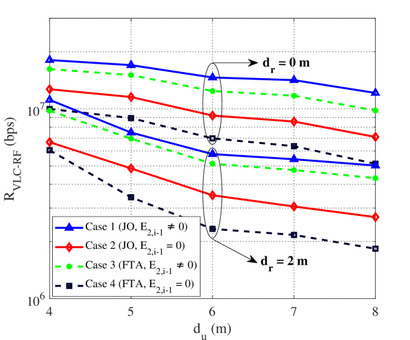
Figure 8: The performance of optimal data rate for different user distances when the relay is located at $d_{\textrm{r}}=0$ m.

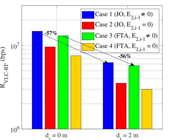
(a) Optimal data rate

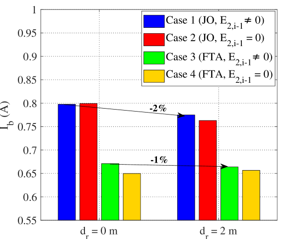
(b) Optimal DC bias

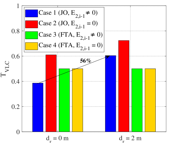
(c) Optimal duration of VLC transmission

Figure 9: The performance of system under consideration with $f_{\textrm{c}}=2.4$ GHz when the user node distance follows ${d_{\textrm{u}}}\sim\mathcal{U}\left[{4,8}\right]$.

• Case 1: Joint optimization (JO) of $I_{\textrm{b}}$ and $T_{\textrm{VLC}}$ with utilizing the harvested energy from previous transmission block;

• Case 2: JO of $I_{\textrm{b}}$ and $T_{\textrm{VLC}}$ without utilizing the harvested energy from previous transmission block (i.e., $E_{2,{i-1}}=0$);

• Case 3: Optimization of $I_{\textrm{b}}$ when $T_{\textrm{VLC}}=T_{\textrm{RF}}=0.5$, i.e., fixed time allocation (FTA), with utilizing the harvested energy from previous transmission block (similar to [7]);

• Case 4: Optimization of $I_{\textrm{b}}$ when $T_{\textrm{VLC}}=T_{\textrm{RF}}=0.5$ (FTA) without utilizing the harvested energy from previous transmission block (i.e., $E_{2,{i-1}}=0$). Similar condition was considered in [13].

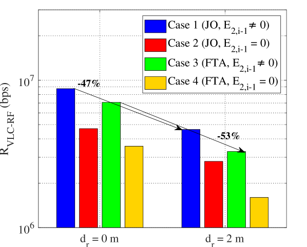
(a) Optimal data rate

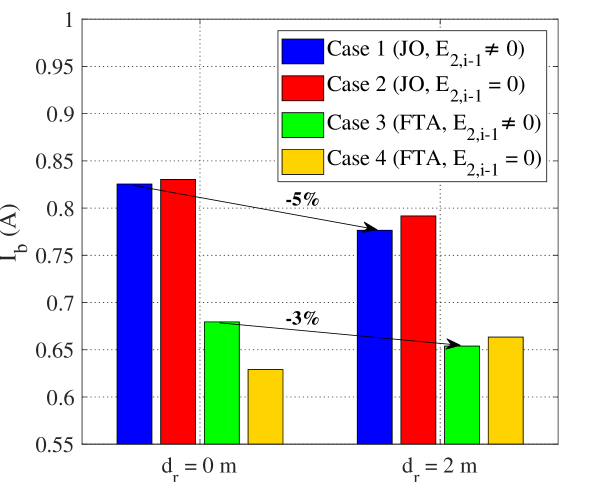
(b) Optimal DC bias

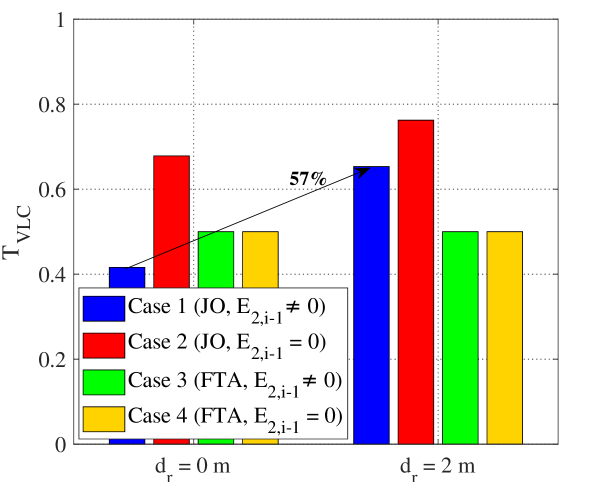
(c) Optimal duration of VLC transmission

Figure 10: The performance of system under consideration with $f_{\textrm{c}}=5$ GHz when the user node distance follows ${d_{\textrm{u}}}\sim\mathcal{U}\left[{4,8}\right]$.

Fig. 8 depicts the performance of optimal data rate when the relay is located at $d_{\textrm{r}}=0$ m and $d_{\textrm{r}}=2$ m. The user distance varies as $d_{\textrm{u}}\in\{4,5,6,7,8\}$ m. We assume RF frequency as ${f_{\textrm{c}}=2.4}$ GHz. It can be observed that Case 1 and Case 3, where the relay can harvest energy during RF transmission, outperform the other cases. Note the optimal data rate for all cases decreases as the user distance increases. Since the relay node is fixed and the achievable information rate is limited by the smaller information rate between the VLC link and the RF link, one can conclude that the restriction in the system under consideration comes from the RF link. In such energy-deprived regimes, harvesting the energy during the second-hop RF transmission (as proposed in our work) benefits significantly in increasing the bottle-necked data rate.

Fig. 9 illustrates the performance of system under consideration assuming the relay location varies as $d_{\textrm{r}}\in\{0,2\}$ m and the user node distance follow Uniform distribution with ${{d_{\textrm{u}}}\sim\mathcal{U}\left[{4,8}\right]}$. Here, the RF frequency is assumed as ${f_{\textrm{c}}=2.4}$ GHz. As it can be observed from Fig. 9(a), solving the joint optimization over $I_{\textrm{b}}$ and $T_{\textrm{VLC}}$ leads to a higher data rate compared with the other considered cases. In addition, Fig. 9(a) clearly shows that harvesting energy during RF transmission (Case 1 and Case 3) results in an increase in optimal data rate. To investigate the reason behind this, we further analyze the optimal DC bias and the time duration assigned for the VLC link in Fig. 9(b) and Fig. 9(c), respectively. The optimal value of DC bias for the joint optimization (regardless of harvesting energy during RF transmission) is higher than the ones obtained when $T_{\textrm{VLC}}=T_{\textrm{RF}}=0.5$ as shown in Fig. 9(b). Recalling $c_{6}^{\prime}$ in (13), this leads to a smaller amount of peak amplitude of the input electrical signal which consequently limits the VLC data rate. In addition, it can be observed that the optimal value of $T_{\textrm{VLC}}$ for Case 1 is less than 0.5 which accordingly restrains the data rate of the VLC link (cf. (2)). Although the difference between the optimal DC bias for Case 1 and Case 2 is practically negligible, optimal $T_{\textrm{VLC}}$ for Case 2 is much higher than Case 1. For Case 2, the power of the relay only relies on the harvested energy during VLC transmission (according to (4)) which can be increased by allocating more time for this phase. This behavior is because Case 2 ignores harvesting energy during RF transmission and allocating more time for VLC transmission aims to compensate for this effect.

To study the effect of RF frequency, Fig. 10 depicts the performance of system under consideration with $f_{\textrm{c}}=5$ GHz when the user node distance follows ${d_{\textrm{u}}}\sim\mathcal{U}\left[{4,8}\right]$ and the relay location varies as $d_{\textrm{r}}\in\{0,2\}$ m. Comparing Fig. 10(a) and Fig. 9(a) shows that the optimal data rate decreases as the RF frequency increases. According to (8), as RF frequency increases the effect of path loss becomes more pronounced. To further investigate the behavior of the optimization problems, the optimal DC bias and the time duration assigned for the VLC link are plotted in Fig. 10(b) and Fig. 10(c), respectively. For Case 1 and Case 2, the optimal DC bias decreases as the relay distance (i.e., $d_{\textrm{r}}$) increases which leads to a decrease in the VLC data rate. Comparing Fig. 10(c) and Fig. 9(c) indicates that the optimal time duration for VLC transmission increases as the RF frequency increases.

7.3 Achievable Data Rate with Relay Random Orientation

(a) Relay location: $d_{\textrm{r}}=0$ m.

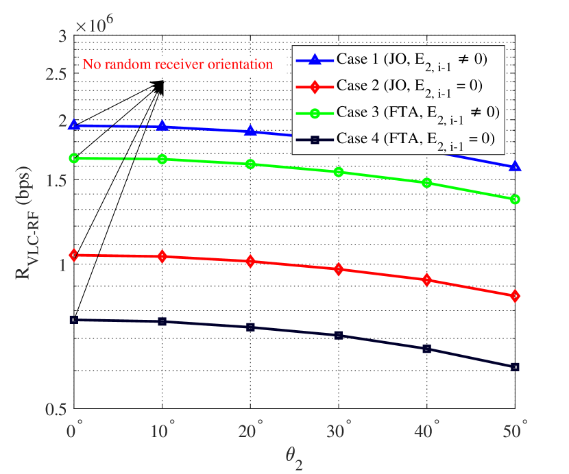
(b) Relay location: $d_{\textrm{r}}=4$ m.

Figure 11: The effect of random orientation on the optimal data rate of the RF user location follows a Uniform distribution with $\mathcal{U}\left[4,8\right]$ when the half-power beamwidth is $\Phi=60^{\circ}$.

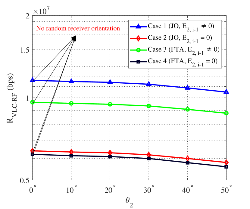
(a) Relay location: $d_{\textrm{r}}=0$ m.

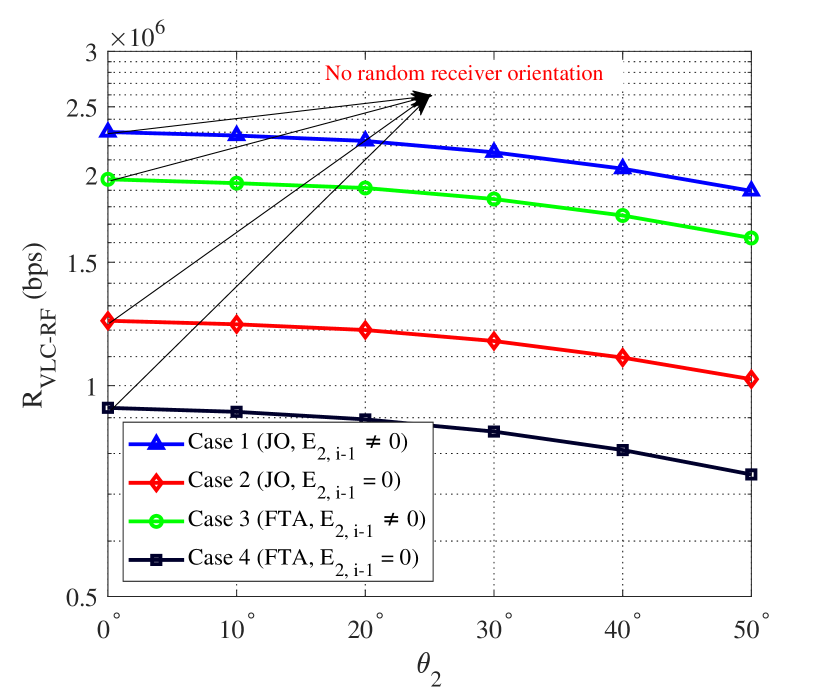
(b) Relay location: $d_{\textrm{r}}=4$ m.

Figure 12: The effect of random orientation on the optimal data rate of the RF user location follows a Uniform distribution with $\mathcal{U}\left[4,8\right]$ when the half-power beamwidth is $\Phi=90^{\circ}$.

In this subsection, we investigate the effect of relay random orientation on the maximum achievable data rate. Similar to the previous subsection, we consider the same transmission policies. Due to the complexity of the expressions for the average data rate of VLC and RF, the optimal values of $T_{\textrm{VLC}}$ and $I_{\textrm{b}}$ are obtained through exhaustive search. We assume the half-power beamwidth as $\Phi=60^{\circ}$, the RF user location follows $d_{u}\sim U[4,8]$ and the RF frequency is considered as ${f_{\textrm{c}}=2.4}$ GHz. In Fig. 11(a), we assume $d_{\textrm{r}}=0$ m whereas the relay distance is set to $d_{\textrm{r}}=4$ m in Fig. 11(b). We assume that $\theta_{\textrm{r}}$ follows $\theta_{\textrm{r}}\sim U[0,\theta_{2}]$ where $\theta_{2}$ varies within the range of $(10^{\circ},50^{\circ})$. As can be seen, the optimal data rate decreases as the range of random orientation increases. It can be readily checked that increasing $\theta_{\textrm{r}}$ leads to a decrease in the VLC channel gain (i.e., (20)). This also affects the harvested energy in the relay node which is further utilized to empower the RF link. The results also reveal the benefit of harvesting energy during RF transmission (Case 1 and Case 3) in increasing the optimal data rate. Our proposed scheme outperforms others since it is able to adjust the VLC link time duration (i.e., $T_{\textrm{VLC}}$) in addition to DC bias (i.e., $I_{\textrm{b}}$). This effect becomes more pronounced when the VLC channel gain decreases (i.e., the relay is farther from the LED). In this case, the system fails to satisfy the data rate threshold (i.e., $10^{6}$ b/s) if it ignores the harvesting energy during RF transmission and/or adjusts the VLC link time duration.

In Fig. 12, we investigate the effect of Lambertian order on the achievable data rate. Specifically, we consider the half-power beamwidth as $\Phi=90^{\circ}$. As it can be seen from Fig. 12(a), the maximum achievable data rate decreases as the half-power beamwidth increases when $d_{\textrm{r}}=0$ m. As the relay distance increases, the effect of random orientation becomes more pronounced. Comparing the results in Fig. 11(b) and Fig. 12(b), it can be observed that the achievable data rate increases as the half-power beamwidth increases.

8 Conclusion

In this paper, we proposed an EH hybrid VLC-RF scheme where the relay harvests energy both during VLC transmission and RF communication. With DF relaying assumed, we have formulated the optimization problem to maximize the achievable data rate. In addition to the DC bias, we considered the assigned time duration for VLC transmission as a design parameter. Specifically, the joint optimization problem was divided into two sub-problems and solved cyclically. Our first sub-problem involved fixing the time duration for VLC transmission and solving the non-convex DC bias problem using MM approach. In the second sub-problem, we solved the optimization problem for the assigned VLC link time duration using the DC bias obtained in the previous step. Furthermore, we investigated the effect of random receiver orientation for the relay on the achievable data rate. Assuming a uniform random distribution, we derived the closed-form expressions for both VLC and RF data rates. Due to the complexity of the problem, the optimization was solved through an exhaustive search. The results have shown that our proposed joint optimization approach achieves a higher data rate compared to solely optimizing the DC bias. We have also observed that the effect of random orientation becomes more pronounced as the relay distance increases. Moreover, while the larger half-power beamwidth leads to a reduction in the achievable data rate when the relay distance is small, it can be beneficial to maintain the achievable data rate as the relay distance increases. Potential future research directions include developing hardware design, considering imperfect channel impulse response, and investigating practical scenarios. For example, investigating the utilization of cooperative communication becomes pertinent, particularly when the end user can opportunistically leverage information from both VLC and RF sources. Furthermore, taking into account the probability of blockages affecting the VLC link while the end user maintains access to both VLC and RF communication channels, such as WiFi, presents a compelling avenue for further exploration.

References

- Raouf et al. [2022] A. H. F. Raouf, C. K. Anjinappa, and I. Guvenc, “Optimal design of energy-harvesting hybrid VLC/RF networks,” in IEEE Globecom Workshops (GC Wkshps), 2022, pp. 705–710.
- Matheus et al. [2019] L. E. M. Matheus, A. B. Vieira, L. F. Vieira, M. A. Vieira, and O. Gnawali, “Visible light communication: Concepts, applications and challenges,” IEEE Commun. Surveys Tuts., vol. 21, no. 4, pp. 3204–3237, 2019.
- Burchardt et al. [2014] H. Burchardt, N. Serafimovski, D. Tsonev, S. Videv, and H. Haas, “VLC: Beyond point-to-point communication,” IEEE Commun. Mag., vol. 52, no. 7, pp. 98–105, 2014.
- Basnayaka and Haas [2015] D. A. Basnayaka and H. Haas, “Hybrid RF and VLC systems: Improving user data rate performance of VLC systems,” in Proc. IEEE Vehicular Technology Conference (VTC), Glasgow, U.K., May 2015, pp. 1–5.
- Delgado-Rajo et al. [2020] F. Delgado-Rajo, A. Melian-Segura, V. Guerra, R. Perez-Jimenez, and D. Sanchez-Rodriguez, “Hybrid RF/VLC network architecture for the Internet of Things,” Sensors, vol. 20, no. 2, p. 478, 2020.
- Pan et al. [2019a] G. Pan, P. D. Diamantoulakis, Z. Ma, Z. Ding, and G. K. Karagiannidis, “Simultaneous lightwave information and power transfer: Policies, techniques, and future directions,” IEEE Access, vol. 7, pp. 28 250–28 257, 2019.
- Rakia et al. [2016] T. Rakia, H.-C. Yang, F. Gebali, and M.-S. Alouini, “Optimal design of dual-hop VLC/RF communication system with energy harvesting,” IEEE Commun. Lett., vol. 20, no. 10, pp. 1979–1982, 2016.
- Yapıcı and Güvenç [2020] Y. Yapıcı and İ. Güvenç, “Energy-vs spectral-efficiency for energy-harvesting hybrid RF/VLC networks,” in Proc. Asilomar Conference on Signals, Systems, and Computers, Pacific Grove, CA, Nov. 2020, pp. 1152–1156.
- Pan et al. [2017] G. Pan, J. Ye, and Z. Ding, “Secure hybrid VLC-RF systems with light energy harvesting,” IEEE Trans. Commun., vol. 65, no. 10, pp. 4348–4359, 2017.
- Zhang et al. [2018] C. Zhang, J. Ye, G. Pan, and Z. Ding, “Cooperative hybrid VLC-RF systems with spatially random terminals,” IEEE Trans. Commun., vol. 66, no. 12, pp. 6396–6408, 2018.
- Pan et al. [2019b] G. Pan, H. Lei, Z. Ding, and Q. Ni, “3-D hybrid VLC-RF indoor IoT systems with light energy harvesting,” IEEE Trans. Green Commun. Netw., vol. 3, no. 3, pp. 853–865, 2019.
- Peng et al. [2020] H. Peng, Q. Li, A. Pandharipande, X. Ge, and J. Zhang, “Performance analysis of a SLIPT-based hybrid VLC/RF system,” in Proc. IEEE/CIC Int. Conf. Commun. China (ICCC), Chongqing, China, Aug. 2020, pp. 360–365.
- Peng et al. [2021] ——, “End-to-end performance optimization of a dual-hop hybrid VLC/RF IoT system based on SLIPT,” IEEE Internet Things J., vol. 8, no. 24, pp. 17 356–17 371, 2021.
- Zhang et al. [2021] Z. Zhang, Q. Li, H. Peng, A. Pandharipande, X. Ge, and J. Zhang, “A SLIPT-based hybrid VLC/RF cooperative communication system with relay selection,” in Proc. IEEE/CIC Int. Conf. Commun. China (ICCC), Chongqing, China, 2021, pp. 277–282.
- Zargari et al. [2021] S. Zargari, M. Kolivand, S. A. Nezamalhosseini, B. Abolhassani, L. R. Chen, and M. H. Kahaei, “Resource allocation of hybrid VLC/RF systems with light energy harvesting,” IEEE Trans. Green Commun. Netw., 2021.
- Xiao et al. [2021] Y. Xiao, P. D. Diamantoulakis, Z. Fang, L. Hao, Z. Ma, and G. K. Karagiannidis, “Cooperative hybrid VLC/RF systems with SLIPT,” IEEE Trans. Commun., vol. 69, no. 4, pp. 2532–2545, 2021.
- Rallis et al. [2023] K. G. Rallis, V. K. Papanikolaou, S. A. Tegos, A. A. Dowhuszko, P. D. Diamantoulakis, M.-A. Khalighi, and G. K. Karagiannidis, “RSMA inspired user cooperation in hybrid VLC/RF networks for coverage extension,” in IEEE Wireless Communications and Networking Conference (WCNC), 2023, pp. 1–6.
- Tran et al. [2019] H.-V. Tran, G. Kaddoum, P. D. Diamantoulakis, C. Abou-Rjeily, and G. K. Karagiannidis, “Ultra-small cell networks with collaborative RF and lightwave power transfer,” IEEE Trans. Commun., vol. 67, no. 9, pp. 6243–6255, 2019.
- Guo et al. [2021] Y. Guo, K. Xiong, Y. Lu, D. Wang, P. Fan, and K. B. Letaief, “Achievable information rate in hybrid VLC-RF networks with lighting energy harvesting,” IEEE Trans. Commun., vol. 69, no. 10, pp. 6852–6864, 2021.
- Diamantoulakis et al. [2018] P. D. Diamantoulakis, G. K. Karagiannidis, and Z. Ding, “Simultaneous lightwave information and power transfer (SLIPT),” IEEE Trans. Green Commun. Netw., vol. 2, no. 3, pp. 764–773, 2018.
- Eroglu et al. [2019] Y. S. Eroglu, C. K. Anjinappa, I. Guvenc, and N. Pala, “Slow beam steering and NOMA for indoor multi-user visible light communications,” IEEE Trans. Mobile Comput., vol. 20, no. 4, pp. 1627–1641, 2019.
- Sun et al. [2016] Y. Sun, P. Babu, and D. P. Palomar, “Majorization-minimization algorithms in signal processing, communications, and machine learning,” IEEE Trans. Signal Process., vol. 65, no. 3, pp. 794–816, 2016.
- Eroğlu et al. [2018] Y. S. Eroğlu, Y. Yapıcı, and I. Güvenç, “Impact of random receiver orientation on visible light communications channel,” IEEE Trans. Commun., vol. 67, no. 2, pp. 1313–1325, 2018.
- Fu et al. [2021] X.-T. Fu, R.-R. Lu, and J.-Y. Wang, “Realistic performance analysis for visible light communication with random receivers,” JOSA A, vol. 38, no. 5, pp. 654–662, 2021.
- Soltani et al. [2019] M. D. Soltani, A. A. Purwita, I. Tavakkolnia, H. Haas, and M. Safari, “Impact of device orientation on error performance of LiFi systems,” IEEE Access, vol. 7, pp. 41 690–41 701, 2019.
- Soltani et al. [2018] M. D. Soltani, A. A. Purwita, Z. Zeng, H. Haas, and M. Safari, “Modeling the random orientation of mobile devices: Measurement, analysis and LiFi use case,” IEEE Trans. Commun., vol. 67, no. 3, pp. 2157–2172, 2018.
- Purwita et al. [2018] A. A. Purwita, M. D. Soltani, M. Safari, and H. Haas, “Impact of terminal orientation on performance in LiFi systems,” in IEEE Wireless Communications and Networking Conference (WCNC), 2018, pp. 1–6.
- Rodoplu et al. [2020] V. Rodoplu, K. Hocaoğlu, A. Adar, R. O. Çikmazel, and A. Saylam, “Characterization of line-of-sight link availability in indoor visible light communication networks based on the behavior of human users,” IEEE Access, vol. 8, pp. 39 336–39 348, 2020.
- Komine and Nakagawa [2003] T. Komine and M. Nakagawa, “Integrated system of white LED visible-light communication and power-line communication,” IEEE trans. Consum. Electron., vol. 49, no. 1, pp. 71–79, 2003.
- Rappaport et al. [1996] T. S. Rappaport et al., Wireless communications: Principles and practice. prentice hall PTR New Jersey, 1996, vol. 2.
- Boyd and Vandenberghe [2004] S. P. Boyd and L. Vandenberghe, Convex optimization. Cambridge university press, 2004.
- Hanzo et al. [2012] L. Hanzo, H. Haas, S. Imre, D. O’Brien, M. Rupp, and L. Gyongyosi, “Wireless myths, realities, and futures: From 3G/4G to optical and quantum wireless,” Proceedings of the IEEE, vol. 100, no. Special Centennial Issue, pp. 1853–1888, 2012.
- Wang et al. [2018] J.-Y. Wang, C. Liu, J.-B. Wang, Y. Wu, M. Lin, and J. Cheng, “Physical-layer security for indoor visible light communications: Secrecy capacity analysis,” IEEE Trans. Commun., vol. 66, no. 12, pp. 6423–6436, 2018.
- Winkler [2016] F. Winkler, “Commutative algebra and algebraic geometry,” Lecture Notes, p. 2005, 2016.
- Gradshteyn and Ryzhik [2014] I. S. Gradshteyn and I. M. Ryzhik, Table of integrals, series, and products. Academic press, 2014.
- [36] WolframAlpha, https://www.wolframalpha.com.