Offline Learning in Markov Games
with General Function Approximation

Abstract

We study offline multi-agent reinforcement learning (RL) in Markov games, where the goal is to learn an approximate equilibrium—such as Nash equilibrium and (Coarse) Correlated Equilibrium—from an offline dataset pre-collected from the game. Existing works consider relatively restricted tabular or linear models and handle each equilibria separately. In this work, we provide the first framework for sample-efficient offline learning in Markov games under general function approximation, handling all 3 equilibria in a unified manner. By using Bellman-consistent pessimism, we obtain interval estimation for policies’ returns, and use both the upper and the lower bounds to obtain a relaxation on the gap of a candidate policy, which becomes our optimization objective. Our results generalize prior works and provide several additional insights. Importantly, we require a data coverage condition that improves over the recently proposed “unilateral concentrability”. Our condition allows selective coverage of deviation policies that optimally trade-off between their greediness (as approximate best responses) and coverage, and we show scenarios where this leads to significantly better guarantees. As a new connection, we also show how our algorithmic framework can subsume seemingly different solution concepts designed for the special case of two-player zero-sum games.

1 Introduction

Offline RL aims to learn a good policy from a pre-collected historical dataset. It has emerged as an important paradigm for bringing RL to real-life scenarios due to its non-interative nature, especially in applications where deploying adaptive algorithms in the real system is financially costly and/or ethically problematic [Levine et al., 2020]. While offline RL has been extensively studied in the single-agent setting, many real-world applications involve the strategic interactions between multiple agents. This renders the necessity of bringing in game-theoretic reasoning, often modeled using Markov games Shapley [1953] in the RL theory literature. Markov games can be viewed as the multi-agent extension of Markov Decision Processes (MDPs), where agents share the same state information and the dynamics is determined by the joint action of all agents.

While online RL in Markov games has seen significant developments in recent years Bai and Jin [2020], Liu et al. [2021], Song et al. [2021], Jin et al. [2021b], offline learning in Markov games has only started to attract attention from the community. Earlier works Cui and Du [2022b], Zhong et al. [2022] focus on tabular cases or linear function approximation, which cannot handle complex environments that require advanced function-approximation techniques. Although there has been a rich literature on single-agent RL with general function approximation Jiang et al. [2017], Jin et al. [2021a], Wang et al. [2020], Huang et al. [2021a], whether and how they can be extended to offline Markov games remains largely unclear. In addition, the learning goal in Markov games is no longer return optimization, but instead finding an equilibrium. However, there are multiple popular notions of equilibria, and prior results for the offline setting mainly focus on one of them (Nash) Cui and Du [2022a, b], Zhong et al. [2022]. These considerations motivate us to study the following question:

Can we design sample-efficient algorithms for offline Markov games with general function approximation, and handle different equilibria in a unified framework?

Unified framework

In this paper, we provide information-theoretic results that answer the question in the positive. We first express the equilibrium gap—the objective we wish to minimize—in a unified manner for 3 popular notions of equilibria: Nash Equilibrium (NE), Correlated Equilibrium (CE), and Coarse Correlated Equilibrium (CCE) (Section 3). Then, we build on top of the Bellman-consistent pessimism framework from single-agent offline RL [Xie et al., 2021a], which allows us to construct confidence sets for policy evaluation and obtain the confidence intervals of policies’ returns. An important difference is that Xie et al. [2021a] only needs pessimistic evaluations in the single-agent case; in contrast, we need both optimistic and pessimistic evaluations to further compute a surrogate upper bound on the equilibrium gap of each candidate policy, which provably leads to strong offline learning guarantees (Section 4).

New insights on data conditions

Our algorithm and analyses also shed new light on the offline learnability of Markov games. In single-agent offline RL, it is understood that a good policy can be learned as long as the data covers one, and this condition is generally known as “single-policy concentrability/coverage” Jin et al. [2021c], Zhan et al. [2022]. In contrast, in Markov games, data covering an equilibrium is intuitively insufficient, as a fundamental aspect of equilibrium is reasoning about what would happen if other agents were to deviate. To address this discrepancy, a notion of “unilateral concentrability” is proposed as a sufficient data condition for offline Markov games Cui and Du [2022a] (see also Zhong et al. [2022]), which asserts that the equilibrium as well as its all unilateral deviations are covered. While this is sufficient and in the worst-case necessary, it remains unclear whether less stringent conditions may also suffice. Our work relaxes the assumption and provide more flexible guarantees. Instead of depending on the worst-case estimation error of all unilateral deviation policies, our error bound exhibits the trade-off between a policy coverage error term and a policy suboptimality term. It automatically adapts to the optimal trade-off, and we show scenarios in Appendix B where the bound significantly improves over unilateral coverage results Cui and Du [2022b].

V-type variant

Our main algorithm estimates the policies’ Q-functions, which takes all agents’ actions as inputs. When specialized to the tabular setting, this would incur an exponentially dependence on the number of agents. While this can be avoided by using strong function approximation to generalize over the joint action space Zhong et al. [2022], it prevents us from reproducing and subsuming the prior works Cui and Du [2022a, b]. To address this issue, we propose a V-type variant of our algorithm, which estimates state-value functions instead and uses importance sampling to correct for action mismatches. It naturally avoids the exponential dependence, and reproduces the rate (up to minor differences) of Cui and Du [2022b] whose analysis is specialized to tabular settings (Section 5).

New connection for two-player zero-sum games

As an additional discovery, we show interesting connection between our work and prior algorithmic ideas [Jin et al., 2022, Cui and Du, 2022b] that are specifically designed for two-player zero-sum games. While they seem very different at the first glance, we show in Appendix B that these ideas can be subsumed by our algorithmic framework and our analyses and guarantees extend straightforwardly.

1.1 Related Work

Offline RL

Offline RL aims to learn a good policy from a pre-collected dataset without direct interaction with the environment. There are many prior works studying single-agent offline RL problem in both the tabular [Yin et al., 2021b, a, Yin and Wang, 2021, Rashidinejad et al., 2021, Xie et al., 2021b, Shi et al., 2022, Li et al., 2022] and function approximation setting Antos et al. [2008], Precup [2000], Chen and Jiang [2019], Xie and Jiang [2020, 2021], Xie et al. [2021a], Jin et al. [2021c], Zanette et al. [2021], Uehara and Sun [2021], Yin et al. [2022], Zhan et al. [2022]. Notably, Xie et al. [2021a] introduces the notion of Bellman-consistent pessimism and our techniques are built on it.

Markov games

Markov games is a widely used framework for multi-agent reinforcement learning. Online learning equilibria of Markov games has been extensively studied, including two-player zero-sum Markov games Wei et al. [2017], Bai and Jin [2020], Bai et al. [2020], Liu et al. [2021], Dou et al. [2022], and multi-player general-sum Markov games Liu et al. [2021], Song et al. [2021], Jin et al. [2021b], Mao and Başar [2022]. Three equilibria are usually considered as the learning goal—Nash Equilibrium (NE), Correlated Equilibrium (CE) and Coarse Correlated Equilibrium (CCE). Recently, a line of works consider solving Markov games with function approximation, including linear Xie et al. [2020], Chen et al. [2022] and general function approximation Huang et al. [2021b], Jin et al. [2022]. A closely related work is Jin et al. [2022], where a multi-agent version of the Bellman-Eluder dimension is introduced to solve zero-sum Markov games under general function approximation. However, they focus on the online setting which is different from our offline setting.

Offline Markov games

Since Cui and Du [2022a]’s initial work on offline tabular zero-sum Markov games, there have been several follow-up works on offline Markov games, either for tabular zero-sum / general-sum Markov games [Cui and Du, 2022b, Yan et al., 2022] or linear function approximation [Zhong et al., 2022, Xiong et al., 2022]. In this work, we study general function approximation for multi-player general-sum Markov games, which is a more general framework. Technically, we differ from these prior works in how we handle uncertainty quantification in policy evaluation, an important technical aspect of offline learning: we use initial state optimism/pessimism for policy evaluation, whereas previous works rely on pre-state pessimism with bonus terms. In addition, previous works require the so-called “unilateral concentrability” assumption of data coverage. Although this assumption is unavoidable for the worst-case, our approach requires a condition that is never worse (and coincides in the worst-case) and can be significantly better on certain instances.

2 Preliminaries

Notations

We use $\Delta(\cdot)$ to denote the probability simplex. We use bold letters to denote vectors such as $\mathbf{a}$ and the $j^{\mathrm{th}}$ element of $\mathbf{a}$ is denoted by $\mathbf{a}_{j}$. We use $-i$ to denote all the players except player $i$. For a positive integer $m$, $[m]$ denotes the set $\{1,2,\cdots,m\}$. $\|f\|_{2,d}^{2}$ represents $\mathbb{E}_{d}[f^{2}]$ and $f(s,\pi)$ stands for $\mathbb{E}_{a\sim\pi(\cdot|s)}[f(s,a)]$. We use $\mathcal{O}(\cdot)$ to hide absolute constants and use $\widetilde{\mathcal{O}}(\cdot)$ to hide logarithmic factors.

2.1 Multi-player General-sum Markov Games

We consider multi-player general-sum Markov games in the infinite-horizon discounted setting. Such a Markov game is specified by $(\mathcal{S},\mathcal{A}=\prod_{i\in[m]}\mathcal{A}_{i},P,r,\gamma,s_{0})$, where $\mathcal{S}$ is the state space with $|\mathcal{S}|=S$, $\mathcal{A}_{i}$ is the action space for player $i$ with $|\mathcal{A}_{i}|=A_{i}$, $\mathbf{a}\in\mathcal{A}$ is the joint action taken by all $m$ players, $P:\mathcal{S}\times\mathcal{A}\rightarrow\Delta(\mathcal{S})$ is the transition function and $P(\cdot|s,\mathbf{a})$ describes the probability distribution over the next state when joint action $\mathbf{a}$ is taken at state $s$, $r=\{r_{i}\}_{i\in[m]}$ is the collection of reward function where $r_{i}:\mathcal{S}\times\mathcal{A}\rightarrow[0,R_{\max}]$ is the deterministic reward function for player $i$, $\gamma\in[0,1)$ is the discount factor, and $s_{0}$ is the fixed initial state which is without loss of generality.

Product and correlated policies

A Markov joint policy $\pi:\mathcal{S}\rightarrow\Delta(\mathcal{A})$ specifies the decision-making strategies of all players and induces a trajectory $s_{0},\mathbf{a}_{0},\mathbf{r}_{0},s_{1},\mathbf{a}_{1},\mathbf{r}_{1},\cdots,s_{t},\mathbf{a}_{t},\mathbf{r}_{t},\cdots$, where $\mathbf{a}_{t}\sim\pi(\cdot|s_{t})$, $\mathbf{r}_{t,i}=r_{i}(s_{t},\mathbf{a}_{t})$, and $s_{t+1}\sim P(\cdot|s_{t},\mathbf{a}_{t})$. For a joint policy $\pi$, $\pi_{i}$ is the marginalized policy of player $i$ and $\pi_{-i}$ is the marginalized policy for the remaining players. A joint policy $\pi$ is a product policy if $\pi=\pi_{1}\times\pi_{2}\times\cdots\pi_{m}$ where each player $i$ takes actions independently according to $\pi_{i}$. If $\pi$ is not a joint policy, sometimes we say $\pi$ is correlated, and the players need to depend their actions on public randomness.

Value function and occupancy

For player $i$ and joint policy $\pi$, we define the value function $V^{\pi}_{i}(s)\coloneqq\mathbb{E}_{\pi}[\sum_{t=0}^{\infty}\gamma^{t}r_{i}(s_{t},\mathbf{a}_{t})|s_{0}=s]$ and the Q-function $Q^{\pi}_{i}(s,\mathbf{a})\coloneqq\mathbb{E}_{\pi}[\sum_{t=0}^{\infty}\gamma^{t}r_{i}(s_{t},\mathbf{a}_{t})|s_{0}=s,a_{0}=\mathbf{a}]$, they are bounded in $[0,V_{\max}]$ where $V_{\max}=R_{\max}/(1-\gamma)$. For each joint policy $\pi$, the policy-specific Bellman operator of the $i^{\mathrm{th}}$ player $\mathcal{T}^{\pi}_{i}:\mathbb{R}^{\mathcal{S}\times\mathcal{A}}\rightarrow\mathbb{R}^{\mathcal{S}\times\mathcal{A}}$ is defined as

$$(\mathcal{T}^{\pi}_{i}f)(s,\mathbf{a})=r_{i}(s,\mathbf{a})+\gamma\mathbb{E}_{s^{\prime}\sim P(\cdot|s,\mathbf{a})}[f(s^{\prime},\pi)],$$

and $Q^{\pi}_{i}$ is the unique fixed point of $\mathcal{T}^{\pi}_{i}$. Note that once a policy is fixed, the game-theoretic considerations are no longer relevant and the value functions are defined in familiar manners similar to the single-agent setting, with the only difference that each player $i$ has its own value function due to the player-specific reward function $r_{i}$. Similar to the single-agent case, we also consider the discounted state-action occupancy $d^{\pi}(s,\mathbf{a})\in\Delta(\mathcal{S}\times\mathcal{A})$ which is defined as $d^{\pi}(s,\mathbf{a})=(1-\gamma)\mathbb{E}_{\pi}[\sum_{t=0}^{\infty}\gamma^{t}\mathbb{I}[s_{t}=s,\mathbf{a}_{t}=\mathbf{a}]]$.

2.2 Offline learning of Markov games

In the offline learning setting, we assume access to a pre-collected dataset and cannot have further interactions with the environment. The offline dataset $\mathcal{D}$ consists of $n$ independent tuples $(s,\mathbf{a},\mathbf{r},s^{\prime})$, which are generated as $(s,\mathbf{a})\sim d_{D}$, $\mathbf{r}_{i}\sim r_{i}(s,\mathbf{a})$ and $s^{\prime}\sim P(\cdot|s,\mathbf{a})$ with some data distribution $d_{D}\in\Delta(\mathcal{S}\times\mathcal{A})$.

Policy class

In practical problems with large state spaces, the space of all possible Markov joint policies is prohibitively large and intractable to work with. To address this, we assume we have a pre-specified policy class $\Pi\subset(\mathcal{S}\to\Delta(\mathcal{A}))$, from which we seek a policy that is approximately an equilibrium under a given criterion. Let $\Pi_{i}=\{\pi_{i}:\pi\in\Pi\}$ denote the class of induced marginalized policies for player $i$, and define $\Pi_{-i}$ similarly.

The extended class

As we will see in Section 3, a fundamental aspect of equilibria is the counterfactual reasoning of how other agents would deviate and respond to a given policy. After considering the possible deviation behaviors of player $i$ in response to each policy $\pi\in\Pi$, we arrive at an extended class $\Pi^{\mathrm{ext}}_{i}\supseteq\Pi$ for player $i$. The concrete form of $\Pi^{\mathrm{ext}}_{i}$ will be defined in Section 3 and can depend on the notion of equilibrium under consideration, and for now it suffices to say that $\Pi^{\mathrm{ext}}_{i}$ is a superset of $\Pi$ consisting of all policies that player $i$ needs to reason about.

Value-function approximation We use $\mathcal{F}_{i}\subset(\mathcal{S}\times\mathcal{A}\rightarrow[0,V_{\max}])$ to approximate the Q-function $Q^{\pi}_{i}$ for each player $i$. Following Xie et al. [2021a], we make two standard assumptions on $\mathcal{F}_{i}$,

Assumption A (Approximate Realizability).

For any player $i\in[m]$ and any $\pi\in\Pi^{\mathrm{ext}}_{i}$, we have

$$\inf_{f\in\mathcal{F}_{i}}\sup_{\text{admissible }d}\left\|f-\mathcal{T}_{i}^{\pi}f\right\|_{2,d}^{2}\leq\varepsilon_{\mathcal{F}},$$

A data distribution $d$ is admissible if $d\in\{d^{\pi^{\prime}}:\pi^{\prime}\in\Pi^{\mathrm{ext}}_{i}\}\cup d_{D}$.

For each player $i$ and joint policy $\pi$, A requires that there exists $f\in\mathcal{F}_{i}$ such that $f$ has small Bellman error under all possible distributions induced from the extended policy class $\Pi^{\mathrm{ext}}_{i}$ and the data distribution. When $Q^{\pi}_{i}\in\mathcal{F}_{i}$, $\forall\pi\in\Pi,i\in[m]$, we have $\varepsilon_{\mathcal{F}}=0$.

Assumption B (Approximate Completeness).

For any player $i\in[m]$ and any $\pi\in\Pi^{\mathrm{ext}}_{i}$, we have

$$\sup_{f\in\mathcal{F}_{i}}\inf_{f^{\prime}\in\mathcal{F}_{i}}\left\|f^{\prime}-\mathcal{T}_{i}^{\pi}f\right\|_{2,d_{D}}^{2}\leq\varepsilon_{\mathcal{F},\mathcal{F}}.$$ (1)

B requires that $\mathcal{F}_{i}$ is approximately closed under operator $\mathcal{T}_{i}^{\pi}$. Both assumptions are direct extensions of their counterparts that are widely used in the offline RL literature.

Distribution mismatch and data coverage

Similar to Xie et al. [2021a], we use the discrepancy of Bellman error under $\pi$ to measure the distribution mismatch between an arbitrary distribution $d$ and data distribution $d_{D}$:

$$\mathscr{C}(d;d_{D},\mathcal{F}_{i},\pi)\coloneqq\max_{f\in\mathcal{F}_{i}}\frac{\|f-\mathcal{T}_{i}^{\pi}f\|_{2,d}^{2}}{\|f-\mathcal{T}_{i}^{\pi}f\|_{2,d_{D}}^{2}}.$$ (2)

We remark that $\mathscr{C}(d;d_{D},\mathcal{F}_{i},\pi)\leq\sup_{s,\mathbf{a}}\frac{d(s,\mathbf{a})}{d_{D}(s,\mathbf{a})}$, which implies that $\mathscr{C}(d;d_{D},\mathcal{F}_{i},\pi)$ is a tighter measurement than the raw density ratio.

3 Equilibria

We consider three common equilibria in game theory: Nash Equilibrium (NE), Correlated Equilibrium (CE) and Coarse Correlated Equilibrium (CCE). We define the three equilibria in a unified fashion using the concept of response class mappings, so that each equilibrium is defined with respect to the relative best response within each corresponding response class.

A response class mapping $\Pi^{\dagger}(\cdot)$ maps a policy $\pi$ to a policy class, $\Pi^{\dagger}(\pi)\coloneqq\bigcup_{i\in[m]}\Pi_{i}^{\dagger}(\pi)$. Roughly speaking, $\Pi_{i}^{\dagger}(\pi)$ is obtained by taking a candidate policy $\pi$, considering various ways that player $i$ would deviate its behavior from $\pi_{i}$ to $\pi_{i}^{\dagger}$, and re-combining $\pi_{i}^{\dagger}$ and $\pi_{-i}$ into joint policies. The space of possible $\pi_{i}^{\dagger}$ which player $i$ can choose from determines the mapping, and will take different forms under different notions of equilibria, as explained next.

1. A product policy is NE if it satisfies that no player can increase her gain by deviating from her own policy. Therefore, the response class mapping for NE is defined as $\Pi^{\dagger,{\mathrm{NE}}}(\pi):=\{\Pi_{i}^{\dagger,{\mathrm{NE}}}(\pi)\}_{i\in[m]}$, where $\Pi_{i}^{\dagger,{\mathrm{NE}}}(\pi):=\{\pi_{i}^{\dagger}\times\pi_{-i}:\pi_{i}^{\dagger}\in\Pi_{i}\}$. Note that here $\Pi_{i}^{\dagger,{\mathrm{NE}}}$ has no dependence on the input $\pi_{i}$, and player $i$ simply considers using some $\pi_{i}^{\dagger}\in\Pi_{i}$ to replace $\pi_{i}$.

2. A CE is defined by a class of strategy modifications $\Phi=(\Phi_{i})_{i\in[m]}$, where $\Phi_{i}\subseteq(\mathcal{S}\times\mathcal{A}_{i}\rightarrow\mathcal{A}_{i})$ is a set of strategy modifications of the $i^{\mathrm{th}}$ player, and each $\phi_{i}\in\Phi_{i}$ is a mapping $\phi_{i}:\mathcal{S}\times\mathcal{A}_{i}\rightarrow\mathcal{A}_{i}$. For any joint policy $\pi$, the modified policy $\phi_{i}\diamond\pi$ is defined as: at state $s\in\mathcal{S}$, all players sample $\mathbf{a}\sim\pi(\cdot|s)$, the $i^{\mathrm{th}}$ player changes action $\mathbf{a}_{i}$ to $\phi_{i}(s,a_{i})$ and $\mathbf{a}_{-i}$ remains the same. For CE, the response class mapping of each joint policy $\pi$ is defined as $\Pi^{\dagger}(\pi)\coloneqq\{\Pi_{i}^{\dagger}(\pi)\}_{i\in[m]}$, where $\Pi_{i}^{\dagger}(\pi)=\{(\phi_{i}\diamond\pi_{i})\odot\pi_{-i}:\phi_{i}\in\Phi_{i}\}$.

3. CCE is defined for general (i.e., possibly correlated) joint policies and is a relaxation of NE. The only difference is that CCE does not require the candidate policy $\pi$ to be a product policy. Hence, the response class mapping of CCE is the same as that of NE.

With the definition of response class mapping, for $\mathrm{EQ}\in\{\mathrm{NE},\mathrm{CE},\mathrm{CCE}\}$, we define the gap of any joint policy $\pi$ with respect to $\Pi^{\dagger,{\mathrm{EQ}}}(\cdot)$ as

$$\mathrm{Gap}^{\Pi^{\dagger,{\mathrm{EQ}}}}(\pi)\coloneqq\max_{i\in[m]}\max_{\pi^{\dagger}\in\Pi_{i}^{\dagger,{\mathrm{EQ}}}(\pi)}V_{i}^{\pi^{\dagger}}(s_{0})-V_{i}^{\pi}(s_{0}).$$

Now we are ready to present the definitions of three equilibria.

Definition 1 (Equilibria; NE, CE, and CCE).

For $\mathrm{EQ}\in\{\mathrm{NE},\mathrm{CE},\mathrm{CCE}\}$, a joint policy (product for NE) is an $\varepsilon$-EQ with respect to $\Pi^{\dagger,{\mathrm{EQ}}}(\cdot)$, if for the response class $\Pi_{i}^{\dagger,{\mathrm{EQ}}}(\pi)$,

$$\mathrm{Gap}^{\Pi^{\dagger,{\mathrm{EQ}}}}(\pi)\leq\varepsilon.$$

Definition 1 is defined with respect to the policy class $\Pi$ and strategy modification class $\Phi$ (for CE). Throughout the paper, we focus on the theoretical guarantees of such “in-class” notion of gaps, which is a reasonable definition if we assume that all players have limited representation power and must work with restricted policy classes. Under additional assumptions (which we call “strategy completeness”; see Appendix A), such “in-class” gaps can be related to a stronger notion of gap where unrestricted deviation policies are considered for the best response.

With the response class mappings, we also define the extended policy class $\Pi^{\mathrm{ext}}_{i}\coloneqq(\bigcup_{\pi\in\Pi}\Pi_{i}^{\dagger}(\pi))\bigcup\Pi$, which characterizes all possible policies with deviation from the $i^{\mathrm{th}}$ player. In addition, we define $\Pi^{\mathrm{ext}}\coloneqq\bigcup_{i=1}^{m}\Pi^{\mathrm{ext}}_{i}$.

4 Information-Theoretic Results for Multi-player General-sum Markov Games

4.1 Algorithm

As our learning goal is to find a policy $\pi\in\Pi$ with small equilibrium gap $\mathrm{Gap}^{\Pi^{\dagger,{\mathrm{EQ}}}}(\pi)$ (for EQ$\in\{\textrm{NE, CE, CCE}\}$), a natural idea is to simply estimate the gap and minimize it over $\pi\in\Pi$. Unfortunately, we are in the offline setting and only have access to data sampled from an arbitrary data distribution $d_{D}$, which may not provide enough information for evaluating the gap of certain policies.

Since the gap is not always amendable to estimation, we instead seek a surrogate objective that will always be an upper bound on the equilibrium gap of each candidate policy $\pi\in\Pi$. The upper bound should also be tight when the policy is covered by the data and we have sufficient information to determine its gap accurately. To achieve this goal, we recall the definition of gap:

$$\mathrm{Gap}^{\Pi^{\dagger,{\mathrm{EQ}}}}(\pi)\coloneqq\max_{i\in[m]}\max_{\pi^{\dagger}\in\Pi_{i}^{\dagger,{\mathrm{EQ}}}(\pi)}V_{i}^{\pi^{\dagger}}(s_{0})-V_{i}^{\pi}(s_{0}).$$

The key idea in our algorithm is that

$$V_{i}^{\pi^{\dagger}}(s_{0})-V_{i}^{\pi}(s_{0})\leq\overline{V}_{i}^{\pi^{\dagger}}(s_{0})-\underline{V}_{i}^{\pi}(s_{0}),$$

where

• $\overline{V}_{i}^{\pi^{\dagger}}(s_{0})\geq V_{i}^{\pi^{\dagger}}(s_{0})$ is an optimistic evaluation of $\pi^{\dagger}$.

• $\underline{V}_{i}^{\pi}(s_{0})\leq V_{i}^{\pi}(s_{0})$ is an pessimistic evaluation of $\pi$.

With this relaxation, the problem reduces to optimistic and pessimistic policy evaluation, for which we can borrow existing techniques from single-agent RL.

Algorithm 1 Bellman-Consistent Equilibrium Learning (BCEL) from an Offline Dataset

1:  Input: Offline dataset $\mathcal{D}$, parameter $\beta_{f}$, equilibrium $\mathrm{EQ}\in\{\mathrm{NE},\mathrm{CE},\mathrm{CCE}\}$

2:  For each player $i\in[m]$ and policy $\pi\in\Pi^{\mathrm{ext}}_{i}$, construct function version space

$$\mathcal{F}_{i}^{\pi,\beta_{f}}=\{f_{i}\in\mathcal{F}_{i}:\mathcal{E}_{i}(f_{i},\pi;\mathcal{D})\leq\beta_{f}\}.$$ (3)

3:  For each player $i\in[m]$, compute

$$\overline{V}_{i}^{\pi^{\dagger}}(s_{0}) =\max_{f\in\mathcal{F}_{i}^{\pi^{\dagger},\beta_{f}}}f(s_{0},\pi^{\dagger}),\quad\forall\pi^{\dagger}\in\Pi^{\mathrm{ext}}_{i}.$$ (4)

$$\underline{V}_{i}^{\pi}(s_{0}) =\min_{f\in\mathcal{F}_{i}^{\pi,\beta_{f}}}f(s_{0},\pi),\quad\forall\pi\in\Pi.$$ (5)

4:  For each policy $\pi\in\Pi$, compute the estimated gap

$$\widehat{\mathrm{Gap}}_{\mathrm{EQ}}(\pi)\coloneqq\max_{i\in[m]}\max_{\pi^{\dagger}\in\Pi_{i}^{\dagger,{\mathrm{EQ}}}(\pi)}\overline{V}^{\pi^{\dagger}}_{i}(s_{0})-\underline{V}_{i}^{\pi}(s_{0}).$$ (6)

5:  Output $\widehat{\pi}\leftarrow\min_{\pi\in\Pi}\widehat{\mathrm{Gap}}_{\mathrm{EQ}}(\pi)$.

Bellman-consistent pessimism & optimism

We use the Bellman-consistent pessimism framework from Xie et al. [2021a] to construct optimistic and pessimistic policy evaluations. For each player $i$, we first use dataset $\mathcal{D}$ to compute an empirical Bellman error of all function $f_{i}\in\mathcal{F}_{i}$ under Bellman operator $\mathcal{T}^{\pi}_{i}$,

$$\mathcal{E}_{i}(f_{i},\pi;\mathcal{D})\coloneqq\mathcal{L}_{i}(f_{i},f_{i},\pi;\mathcal{D})-\min_{f^{\prime}_{i}\in\mathcal{F}_{i}}\mathcal{L}_{i}(f^{\prime}_{i},f_{i},\pi;\mathcal{D}),$$

$$\mathcal{L}_{i}(f^{\prime}_{i},f_{i},\pi;\mathcal{D})\coloneqq\frac{1}{n}\!\sum_{(s,\mathbf{a},\mathbf{r},s^{\prime})\in\mathcal{D}}\!\!\left(f^{\prime}_{i}(s,\mathbf{a})-\mathbf{r}_{i}-\gamma f_{i}(s^{\prime},\pi)\right)^{2}.$$

Similar to the single-agent setting, $\mathcal{E}_{i}(f_{i},\pi;\mathcal{D})$ is a good approximation of the true Bellman error of $f_{i}$ w.r.t. $\pi$, i.e., $\mathcal{E}_{i}(f_{i},\pi;\mathcal{D})\approx\|f_{i}-\mathcal{T}_{i}^{\pi}f_{i}\|_{2,d_{D}}^{2}$, so we can construct a version space $\mathcal{F}_{i}^{\pi,\beta_{f}}$ for each player $i$ and policy $\pi\in\Pi^{\mathrm{ext}}_{i}$ in Equation 3. To ensure that the best approximation of $Q_{i}^{\pi}$ is contained in $\mathcal{F}_{i}^{\pi,\beta_{f}}$, given a failure probability $\delta>0$, we pick the threshold parameter $\beta_{f}$ as follows,

$$\beta_{f}=\frac{80V_{\max}^{2}\log\frac{|\mathcal{F}||\Pi^{\mathrm{ext}}|}{\delta}}{n}+30\varepsilon_{\mathcal{F}},$$

where $\mathcal{F}=\bigcup_{i=1}^{m}\mathcal{F}_{i}$. Then, optimistic and pessimistic evaluations can be obtained by simply taking the highest and the lowest prediction on the initial state $s_{0}$ across all functions in the version space (Equation 4 and (5)).

With $\overline{V}_{i}^{\pi^{\dagger}}(s_{0})$ and $\underline{V}_{i}^{\pi}(s_{0})$ at hand, we calculate the estimated gap $\widehat{\mathrm{Gap}}_{\mathrm{EQ}}(\pi)$ for each $\pi\in\Pi$ in Equation 6. We select the policy $\widehat{\pi}$ with the lowest estimated gap and the algorithm is summarized in Algorithm 1.

4.2 Theoretical guarantees

Before presenting the theoretical guarantee, we introduce the interval width $\Delta_{i}^{\pi}$ of $\mathcal{F}_{i}^{\pi,\beta_{f}}$, which will play a key role in our main theorem statement:

$$\Delta_{i}^{\pi} \coloneqq\max_{f_{i}\in\mathcal{F}_{i}^{\pi,\beta_{f}}}f_{i}(s_{0},\pi)-\min_{f_{i}\in\mathcal{F}_{i}^{\pi,\beta_{f}}}f_{i}(s_{0},\pi).$$

As we will see, $\Delta_{i}^{\pi}$ is a measure of how well the data distribution $d_{D}$ covers $d^{\pi}$, the state-action occupancy of $\pi$. The better coverage, the smaller $\Delta_{i}^{\pi}$. This is formalized by the following proposition:

Proposition 2 (Bound on interval width).

With probability at least $1-\delta$, for any player $i\in[m]$ and any $\pi\in\Pi^{\mathrm{ext}}_{i}$, we have

$$\Delta_{i}^{\pi}\leq\min_{d}\frac{1}{1-\gamma}\sqrt{\mathscr{C}(d;d_{D},\mathcal{F}_{i},\pi)}\varepsilon_{\mathrm{apx}}+\frac{1}{1-\gamma}\sum_{s,\mathbf{a}}(d^{\pi}\!\setminus\!d)(s,\mathbf{a})\left[\Delta f_{i}^{\pi}(s,\mathbf{a})-\gamma(P^{\pi}\Delta f_{i}^{\pi})(s,\mathbf{a})\right],$$ (7)

where $\varepsilon_{\mathrm{apx}}=\mathcal{O}\left(V_{\max}\sqrt{\frac{\log\frac{|\mathcal{F}||\Pi^{\mathrm{ext}}|}{\delta}}{n}}+\sqrt{\varepsilon_{\mathcal{F}}+\varepsilon_{\mathcal{F},\mathcal{F}}}\right)$, $(d^{\pi}\setminus d)(s,\mathbf{a})\coloneqq\max(d^{\pi}(s,\mathbf{a})-d(s,\mathbf{a}),0)$, $\Delta f^{\pi}_{i}(s,\mathbf{a})\coloneqq f_{i}^{\pi,\max}(s,\mathbf{a})-f_{i}^{\pi,\min}(s,\mathbf{a})$, and $(P^{\pi}f)(s,\mathbf{a})=\mathbb{E}_{s^{\prime}\sim P(\cdot|s,\mathbf{a})}[f(s^{\prime},\pi)]$.

Here, a distribution $d\in\Delta(\mathcal{S}\times\mathcal{A})$ in Equation 7 is introduced to handle the discrepancy between $d_{D}$ and $d^{\pi}$. The first term in Equation 7 captures the distribution mismatch between $d$ and $d_{D}$, and the second term represents the off-support Bellman error under $\pi$. When the data distribution $d_{D}$ has a full coverage on $d^{\pi}$, $d$ can be chosen as $d^{\pi}$ and the second term becomes zero. Therefore, for the purpose of developing intuitions, one can always choose $d=d^{\pi}$ and treat $\Delta_{i}^{\pi}\propto\sqrt{\mathscr{C}(d^{\pi};d_{D},\mathcal{F}_{i},\pi)}$, though in general some $d\neq d^{\pi}$ may achieve a better trade-off and tighter bound.

With an intuitive understanding of $\Delta_{i}^{\pi}$, we are ready to show the following theorem for our proposed algorithm.

Theorem 3.

With probability at least $1-\delta$, for any $\pi\in\Pi$ and $\mathrm{EQ}\in\{\mathrm{NE},\mathrm{CE},\mathrm{CCE}\}$, the output policy $\widehat{\pi}$ of Algorithm 1 satisfies that

$$\mathrm{Gap}^{\Pi^{\dagger,{\mathrm{EQ}}}}(\widehat{\pi})\leq\mathrm{Gap}^{\Pi^{\dagger,{\mathrm{EQ}}}}(\pi)+\frac{4\sqrt{\varepsilon_{\mathcal{F}}}}{1-\gamma}+\max_{i\in[m]}\min_{\widetilde{\pi}_{i}\in\Pi_{i}^{\dagger,{\mathrm{EQ}}}(\pi)}\left(\Delta_{i}^{\widetilde{\pi}_{i}}+\Delta_{i}^{\pi}+\mathrm{subopt}_{i}^{\pi}(\widetilde{\pi}_{i})\right),$$

where $\mathrm{subopt}_{i}^{\pi}(\widetilde{\pi}_{i})\coloneqq\max_{\pi^{\dagger}\in\Pi_{i}^{\dagger}(\pi)}\overline{V}_{i}^{\pi^{\dagger}}(s_{0})-\overline{V}_{i}^{\widetilde{\pi}_{i}}(s_{0})$.

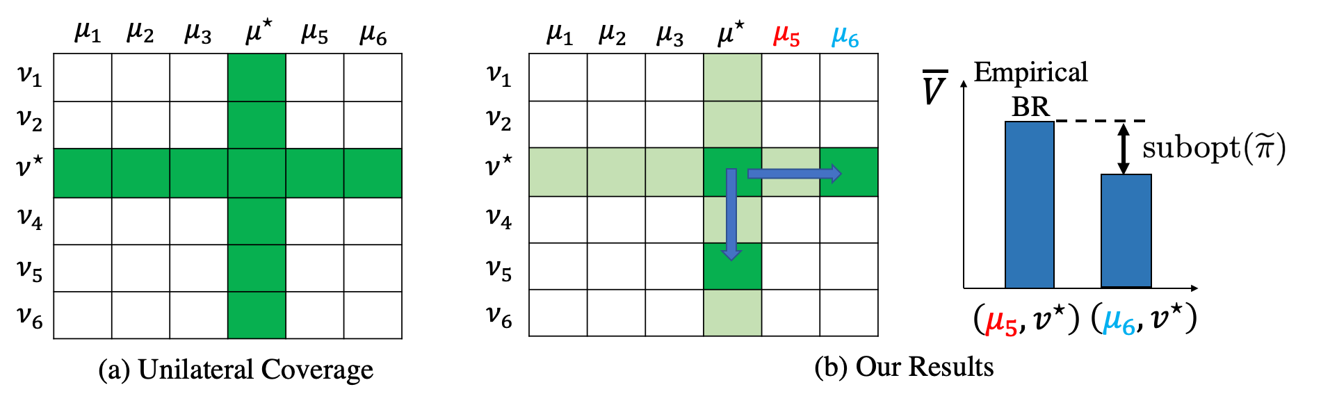
Figure 1: Illustration of unilateral coverage and our results on a zero-sum example. (a) Unilateral coverage requires the dataset to cover all unilateral pairs $(\mu^{\star},\nu^{\prime})$ and $(\mu^{\prime},\nu^{\star})$ where $(\mu^{\star},\nu^{\star})$ is NE. (b) Our approach enjoys an adaptive property and relaxes the condition. To begin with, we can already achieve a good sample complexity if the data were to cover the optimistic best response ($(\mu_{5},\nu^{\star})$ in this example) only, i.e. when $\Delta^{\mu_{5},\nu^{\star}}$ was small. Even when the dataset has a poor coverage on $(\mu_{5},\nu^{\star})$, there may exists some other $\mu_{6}$ so that $\Delta^{\mu_{5},\nu^{\star}}\gg\Delta^{\mu_{6},\nu^{\star}}$. Instead of suffering $\Delta^{\mu_{5},\nu^{\star}}$, our approach automatically adapts to the policy $\widetilde{\pi}=(\mu_{6},\nu^{\star})$ which achieves a better trade-off between the policy coverage term $\Delta^{\widetilde{\pi}}$ and suboptimality term $\mathrm{subopt}(\widetilde{\pi})$.

4.3 Improvement over unilateral coverage

To interpret Theorem 3 and compare it to existing guarantees, we first introduce a direct corollary of Theorem 3 + Proposition 2, which is a relaxed form of our result that is closer to existing guarantees by Cui and Du [2022a, b].

Corollary 4.

For Nash equilibrium policy $\pi^{\star}\in\Pi$, suppose there exists an unilateral coefficient $C(\pi^{\star})$ such that the following inequality holds

$$\max_{i\in[m]}\max_{\pi^{\dagger}\in\Pi_{i}^{\dagger,{\mathrm{NE}}}(\pi^{\star})}\mathscr{C}(d^{\pi^{\dagger}};d_{D},\mathcal{F}_{i},\pi^{\star})\leq C(\pi^{\star}).$$ (8)

With probability at least $1-\delta$, we have

$$\mathrm{Gap}^{\Pi^{\dagger,{\mathrm{NE}}}}(\widehat{\pi})\leq\mathcal{O}\left(\frac{V_{\max}\sqrt{\frac{\log\frac{|\mathcal{F}||\Pi^{\mathrm{ext}}|}{\delta}}{n}}+\sqrt{\varepsilon_{\mathcal{F}}+\varepsilon_{\mathcal{F},\mathcal{F}}}}{1-\gamma}\sqrt{C(\pi^{\star})}\right).$$

The gap bound in Corollary 4 takes a simple form: the first part of it has an $O(1/\sqrt{n})$ statistical error (scaled by the complexities of function and policy classes, as fully expected), and an approximation error term that depends on $\varepsilon_{\mathcal{F}},\varepsilon_{\mathcal{F},\mathcal{F}}$, which goes to $0$ when our function classes are exactly realizable and Bellman-complete.

The key item in the bound is the $\sqrt{C(\pi^{*})}$ factor, which measures distribution mismatch and implicitly determines the data coverage condition. $C(\pi^{*})$ is defined in Equation 8. As we can see, having a small $C(\pi^{*})$ requires that data not only covers $\pi^{*}$ itself, but also all policies in $\Pi_{i}^{\dagger,{\mathrm{NE}}}(\pi^{\star})=\{\pi_{i}\times\pi^{\star}_{-i}:\pi_{i}\in\Pi_{i}\}$. This is the notion of unilateral coverage proposed by Cui and Du [2022a] and Zhong et al. [2022]. Visualizing this in Figure 1(a) with a simplified setting of a two-player matrix game, such a condition corresponds to data covering the entire “cross” centered at the NE.

Although Cui and Du [2022a] argues that unilateral coverage is “sufficient and necessary” in the worst case, their argument does not exclude an improved version that can be substantially relaxed under certain conditions, and we show that our Theorem 3 is such a version. We now provide a breakdown of the bound in Theorem 3:

1. First, the RHS of the bound depends on $\Delta_{i}^{\pi}$, where $\pi$ is the policy we compete with and correspond to $\pi^{*}$ in Corollary 4. Recalling that $\Delta_{i}^{\pi}\propto\sqrt{\mathscr{C}(d^{\pi};d_{D},\mathcal{F}_{i},\pi)}$, this term corresponds to data coverage on $\pi^{*}$, which is always needed if we wish to compete with $\pi^{*}$.

2. The RHS also depends on $\Delta_{i}^{\widetilde{\pi}_{i}}+\mathrm{subopt}_{i}^{\pi}(\widetilde{\pi}_{i})$, where $\widetilde{\pi}_{i}$ is minimized over $\Pi_{i}^{\dagger,{\mathrm{NE}}}(\pi^{\star})$ when EQ=NE (and Equation 8 maximizes over $\pi^{\dagger}$). In particular, we can always choose $\widetilde{\pi}_{i}$ as the policy that maximizes $\overline{V}_{i}$, i.e., the optimistic best response. This would set $\mathrm{subopt}_{i}^{\pi}(\widetilde{\pi}_{i})=0$, showing that we only need coverage for the optimistic best response policy, instead of all policies in $\Pi_{i}^{\dagger,{\mathrm{NE}}}(\pi^{\star})$ as required by the unilateral assumption.

3. Finally, our bound provides a further relaxation: when the optimistic best response is poorly covered, we may choose some other well-covered $\widetilde{\pi}_{i}$ instead, and pay an extra term $\mathrm{subopt}_{i}^{\pi}(\widetilde{\pi}_{i})$ that measures to what extent $\widetilde{\pi}_{i}$ is an approximate $\overline{V}_{i}$-based best response.

Again, we illustrate the flexibility of our bound in Figure 1(b). Below we also show a concrete example, where our guarantee leads to significantly improved sample rates compared to that provided by the unilateral condition.

Example

Consider a simple two-player zero-sum matrix game with payoff matrix:

where the column player aims to maximize the reward and the row player aims to minimize it. It is clear to see $(a_{1},b_{1})$ is NE. The offline dataset $\mathcal{D}$ is collected from the following distribution,

where $0<p_{2}\ll p_{1}$ and $p_{3}=\frac{1-p_{1}-4p_{2}}{4}$. Under Corollary 4 (i.e., unilateral coverage [Cui and Du, 2022a]), the sample complexity bound is $\widetilde{\mathcal{O}}(\frac{1}{p_{2}\epsilon^{2}})$. However, when $n>\widetilde{\mathcal{O}}(\frac{1}{p_{2}})$, we already identify $(a_{1},b_{2})$, $(a_{1},b_{3})$, $(a_{2},b_{1})$, and $(a_{3},b_{1})$ as suboptimal actions with high probability. On this event, Theorem 3 shows that we only suffer the coverage coefficient on the optimistic best response (which is $(a_{1},b_{1})$ itself), so that the sample complexity bound becomes $\widetilde{\mathcal{O}}(\max\{\frac{1}{p_{2}},\frac{1}{p_{1}\epsilon^{2}}\})\ll\widetilde{\mathcal{O}}(\frac{1}{p_{2}\epsilon^{2}})$.

5 V-type Function Approximation

A potential caveat of our approach in Section 4 is that we model Q-functions which take joint actions as inputs. In the tabular setting, the complexity of the full Q-function class has exponential dependence on the number of agents $m$, whereas prior results specialized to tabular settings do not suffer such a dependence.

While it is known that jointly featurizing the actions can avoid such an exponential dependence Zhong et al. [2022] (in a way similar to how linear MDP results do not incur $|\mathcal{A}|$ dependence in the single-agent setting Jin et al. [2020]), in this section we provide an alternative approach that directly subsumes the prior tabular results and produces the same rate (up to minor differences to be discussed). We propose a V-type variant algorithm of BCEL, which directly models the state-value function $V_{i}^{\pi}$ with the help of a function class $\mathcal{G}_{i}\subset(\mathcal{S}\rightarrow[0,V_{\max}])$ for each player $i$.

As before, we assume that the tuples $(s,\mathbf{a},\mathbf{r},s^{\prime})\in\mathcal{D}$ are generated as $(s,\mathbf{a})\sim d_{D}$, $\mathbf{r}_{i}\sim r_{i}(s,\mathbf{a})$ and $s^{\prime}\sim P(\cdot|s,\mathbf{a})$. In this section, we write $d_{D}=d_{S}\times d_{A}$, i.e., $(s,\mathbf{a})\sim d_{D}\Leftrightarrow s\sim d_{S},a\sim d_{A}(\cdot|s)$. We additionally assume that (1) $d_{A}(\mathbf{a}|s)>0,\forall(s,\mathbf{a})\in\mathcal{S}\times\mathcal{A}$, and (2) the behavior policy $d_{A}(\cdot|s)$ is known to the learner. We use the behavior policy to perform importance weighting on the actions to correct the mismatch between $d_{A}$ and $\pi$, and modify the loss function $\mathcal{L}$ as follows: for any function $g_{i}\in\mathcal{G}_{i}$, define

$$\mathcal{L}_{i}(g^{\prime}_{i},g_{i},\pi;\mathcal{D})\coloneqq\frac{1}{n}\sum_{(s,\mathbf{a},\mathbf{r},s^{\prime})\in\mathcal{D}}\frac{\pi(\mathbf{a}|s)}{d_{A}(\mathbf{a}|s)}\left(g^{\prime}_{i}(s,\mathbf{a})-\mathbf{r}_{i}-\gamma g_{i}(s^{\prime},\pi)\right)^{2}.$$

Similarly as before, we compute empirical Bellman error $\mathcal{E}_{i}(g_{i},\pi;\mathcal{D})\coloneqq\mathcal{L}_{i}(g_{i},g_{i},\pi;\mathcal{D})-\min_{g^{\prime}_{i}\in\mathcal{G}_{i}}\mathcal{L}_{i}(g^{\prime}_{i},g_{i},\pi;\mathcal{D})$ and construct version space $\mathcal{G}_{i}^{\pi,\varepsilon}=\{g_{i}\in\mathcal{G}_{i}:\mathcal{E}_{i}(g_{i},\pi;\mathcal{D})\leq\beta_{g}\}$. What is slightly different is that we set parameter $\beta_{g}$ as

$$\beta_{g}\coloneqq\frac{80C_{A}(\pi)V_{\max}^{2}\log\frac{|\mathcal{F}||\Pi^{\mathrm{ext}}|}{\delta}}{n}+30\varepsilon_{\mathcal{F}},$$

where $C_{A}(\pi)\coloneqq\max_{s,\mathbf{a}}\frac{\pi(\mathbf{a}|s)}{d_{A}(\mathbf{a}|s)}$. Compared to $\beta_{f}$ in Algorithm 1, the extra $C_{A}(\pi)$ term comes from importance weighting. With $\mathcal{G}_{i}^{\pi,\beta_{g}}$ at hand, we define

$$g_{i}^{\pi,\max}\coloneqq\mathop{\mathrm{argmax}}_{g_{i}\in\mathcal{G}_{i}^{\pi,\beta_{g}}}g_{i}(s_{0}),\quad g_{i}^{\pi,\min}\coloneqq\mathop{\mathrm{argmin}}_{g_{i}\in\mathcal{G}_{i}^{\pi,\beta_{g}}}g_{i}(s_{0}).$$

We then compute $\widehat{\mathrm{Gap}}_{\mathrm{EQ}}(\pi)$ which is an upper bound on equilibrium gap for any $\pi\in\Pi$:

$$\widehat{\mathrm{Gap}}_{\mathrm{EQ}}(\pi)\coloneqq\max_{i\in[m]}\max_{\pi^{\dagger}\in\Pi_{i}^{\dagger,{\mathrm{EQ}}}(\pi)}g_{i}^{\pi^{\dagger},\max}(s_{0})-g_{i}^{\pi,\min}(s_{0}).$$

We select the policy by minimizing the estimated equilibrium gap:

$$\widehat{\pi}=\mathop{\mathrm{argmin}}_{\pi\in\Pi}\widehat{\mathrm{Gap}}_{\mathrm{EQ}}(\pi),$$ (9)

whose performance guarantee is shown as follows.

Theorem 5 (V-type guarantee).

With probability at least $1-\delta$, for any $\pi\in\Pi$ and $\mathrm{EQ}\in\{\mathrm{NE},\mathrm{CE},\mathrm{CCE}\}$, the output policy $\widehat{\pi}$ from Equation 9 satisfies that

$$\mathrm{Gap}^{\Pi^{\dagger,{\mathrm{EQ}}}}(\widehat{\pi})\leq\mathrm{Gap}^{\Pi^{\dagger,{\mathrm{EQ}}}}(\pi)+\frac{4\sqrt{\varepsilon_{\mathcal{F}}}}{1-\gamma}+\max_{i\in[m]}\min_{\widetilde{\pi}_{i}\in\Pi_{i}^{\dagger,{\mathrm{EQ}}}(\pi)}\left(\Delta_{i}^{\widetilde{\pi}_{i}}+\Delta_{i}^{\pi}+\mathrm{subopt}_{i}^{\pi}(\widetilde{\pi}_{i})\right),$$

where $\Delta_{i}^{\pi}=g_{i}^{\pi,\max}(s_{0})-g_{i}^{\pi,\min}(s_{0})$ and $\mathrm{subopt}_{i}^{\widetilde{\pi}_{i}}=\max_{\pi^{\dagger}\in\Pi_{i}^{\dagger,{\mathrm{EQ}}}(\pi)}g_{i}^{\pi^{\dagger},\max}(s_{0})-g_{i}^{\widetilde{\pi}_{i},\max}(s_{0})$. In addition, with probability at least $1-\delta$, for any player $i\in[m]$ and any $\pi\in\Pi^{\mathrm{ext}}_{i}$, we have

$$\Delta_{i}^{\pi} \leq\min_{d\in\Delta(S)}\frac{1}{1-\gamma}\sqrt{\mathscr{C}(d;d_{S},\mathcal{G}_{i},\pi)}\varepsilon_{\mathrm{apx}}+\frac{1}{1-\gamma}\sum_{s\in\mathcal{S}}(d^{\pi}\setminus d)(s)\left[\Delta g_{i}^{\pi}(s)-\gamma(P_{i}^{\pi}\Delta g_{i}^{\pi})(s)\right],$$

where $\varepsilon_{\mathrm{apx}}=\mathcal{O}\left(V_{\max}\sqrt{C_{A}(\pi)\frac{\log\frac{|\mathcal{G}||\Pi^{\mathrm{ext}}|}{\delta}}{n}}+\sqrt{\varepsilon_{\mathcal{F}}+\varepsilon_{\mathcal{F},\mathcal{F}}}\right)$, $(d^{\pi}\setminus d)(s)\coloneqq\max(d^{\pi}(s)-d(s),0)$, $\Delta g^{\pi}_{i}(s)\coloneqq g_{i}^{\pi,\max}(s)-g_{i}^{\pi,\min}(s)$, and $(P_{i}^{\pi}g)(s)=\mathbb{E}_{\mathbf{a}\sim\pi(\cdot|s),s^{\prime}\sim P(\cdot|s,\mathbf{a})}[r_{i}(s,\mathbf{a})+g(s^{\prime})]$.

Similar to the results in Section 4, our bound enjoys an adaptive property and automatically selects the best policy $\widetilde{\pi}_{i}$, which achieves the trade-off between the suboptimality error $\mathrm{subopt}_{i}^{\pi}(\widetilde{\pi}_{i})$ and the data coverage error $\Delta_{i}^{\widetilde{\pi}_{i}}$. Furthermore, when the dataset $\mathcal{D}$ satisfies the unilateral coverage assumption, we have the following corollary.

Corollary 6.

For Nash equilibrium policy $\pi^{\star}\in\Pi$, if there exists an unilateral coefficient $C_{S}(\pi^{\star})$ such that the following inequality holds

$$\max_{i\in[m]}\max_{\pi^{\dagger}\in\Pi_{i}^{\dagger,{\mathrm{NE}}}(\pi^{\star})}\mathscr{C}(d^{\pi^{\dagger}};d_{S},\mathcal{G}_{i},\pi^{\star})\leq C_{S}(\pi^{\star}).$$ (10)

With probability at least $1-\delta$, we have

$$\mathrm{Gap}^{\Pi^{\dagger,{\mathrm{NE}}}}(\widehat{\pi})\leq\mathcal{O}\left(\frac{V_{\max}\sqrt{\frac{\log\frac{|\mathcal{G}||\Pi^{\mathrm{ext}}|}{\delta}}{n}}+\sqrt{\varepsilon_{\mathcal{F}}+\varepsilon_{\mathcal{F},\mathcal{F}}}}{1-\gamma}\sqrt{C_{A}(\pi^{\star})C_{S}(\pi^{\star})}\right).$$

Compared to Corollary 4, our bound here depends logarithmically on the V-function class $\mathcal{G}$ instead of the Q-function class $\mathcal{F}$. In the tabular setting when we use fully expressive (and stationary) function classes, $\log|\mathcal{G}|\approx\mathcal{O}(S)$ (via a simple covering argument) and thus our bound avoids the exponential dependence on $m$ (i.e., $\prod_{i=1}^{m}A_{i}$ dependence). In comparison, Cui and Du [2022b] established $\widetilde{\mathcal{O}}\left(\sqrt{H^{4}S^{2}\log(\mathcal{N}(\Pi))C(\pi^{\star})/n}\right)$ error bound for finite-horizon tabular Markov games, where $H$ is the horizon length and $\mathcal{N}(\Pi)$ roughly corresponds to our $|\Pi^{\mathrm{ext}}|$. While finite-horizon and discounted results are generally incomparable, under a standard translation, our bound has the same rate $\widetilde{\mathcal{O}}(n^{-1/2})$; $\sqrt{\log|\mathcal{G}|}\approx\sqrt{SH}$ which results in a better dependence on $S$ (saving a $\sqrt{S}$ factor) and a worse overall dependence on $H$ (we have $\sqrt{H^{5}}$). The slight downside is that Corollary 6 measures distribution mismatch on actions and states separately (instead of doing them jointly as $C(\pi^{*})$ in Corollary 4), which is looser.

6 Discussion and Conclusion

Algorithms for two-player zero-sum games

For most part of this paper we consider the general case of multi-player general-sum Markov games. We discover that when our algorithm is specialized to the special case of two-player zero-sum (2p0s), it seemingly differs from another sample-efficient algorithm specifically designed for 2p0s and inspired by Jin et al. [2022], Cui and Du [2022b]. In Appendix B, we show that this difference is superficial, and these specialized algorithms can be subsumed as small variants of our algorithm.

Conclusion and open problems

In this work, we study offline learning in Markov games. We design a framework that learn three popular equilibrium notions in a unified manner under general function approximation. The adaptive property of our framework enables us to relax and achieve significant improvement over the “unilateral concentrability” condition under certain situations.

One open problem is whether one can design a computational efficient algorithm for learning CE/CCE in offline Markov games, even in the tabular setting. A potential direction is to adapt the computationally efficient V-Learning algorithm [Song et al., 2021, Jin et al., 2021b]—which runs no-regret learning dynamics at each state—to the offline setting, which may require new ideas.

Appendix A Connection Between In-class Gap and Real Gap

In this paper we consider “in-class” equilibrium gaps that are defined w.r.t. certain deviation policy classes (Section 3). It is also common to consider stronger notions of equilibrium gap, which we denote simply as $\mathrm{Gap}^{\mathrm{EQ}}$, where the deviation policies are unrestricted, e.g., for NE and CCE, the deviation policies can take arbitrary policies Nash Jr [1996], Aumann [1974].

To establish the connection between our in-class gap and the stronger notion of gap, we have the following strategy completeness assumption,

Assumption C (Strategy completeness).

For any player $i\in[m]$ and any $\mathrm{EQ}\in\{\mathrm{NE},\mathrm{CCE}\}$, we have

$$\max_{\pi^{\dagger}\in\Pi_{i}^{\dagger,{\mathrm{EQ}}}(\pi)}V_{i}^{\pi^{\dagger}}(s_{0})\geq\max_{\pi^{\prime}:\pi^{\prime}_{-i}=\pi_{-i}}V_{i}^{\pi^{\prime}}(s_{0})-\varepsilon_{\Pi}.$$

For $\mathrm{CE}$, we have

$$\max_{\pi^{\dagger}\in\Pi_{i}^{\dagger,{\mathrm{CE}}}(\pi)}V_{i}^{\pi^{\dagger}}(s_{0})\geq\max_{\phi_{i}}V_{i}^{(\phi_{i}\diamond\pi_{i})\odot\pi_{-i}}(s_{0})-\varepsilon_{\Pi}.$$

C requires that the (unrestricted) best-response policy is contained in $\Pi$ (and its counterpart for CE contained in $\Phi$, respectively). Under C, it is clear that for any $\mathrm{EQ}\in\{\mathrm{NE},\mathrm{CE},\mathrm{CCE}\}$ and $\pi$, $\mathrm{Gap}^{\mathrm{EQ}}(\pi)\leq\mathrm{Gap}^{\Pi^{\dagger,{\mathrm{EQ}}}}(\pi)+\varepsilon_{\Pi}$.

Appendix B A Connection in 2-player-0-sum Games

For the most part of this paper, we have considered the general case of multi-player general-sum Markov games. When we are in a specialized setting, such as two-player zero-sum Markov games (2p0s), it is often the case that we can exploit the special structure and come up with alternative algorithms Yan et al. [2022], Jin et al. [2022].

In particular, Cui and Du [2022b, Section 3] design an offline 2p0s algorithm for the tabular setting, and extending their algorithm to the function approximation setting (using uncertainty quantification techniques from our paper) results in an algorithm that seemingly looks very different from our Algorithm 1. However, below we show that despite the superficial difference, the two algorithms are actually quite similar and can be derived using optimism/pessimism in the same way as in our Algorithm 1, with only one minor difference of minimizing the duality gap versus our $\mathrm{Gap}^{{\rm NE}}$. Consequently, for their algorithm, we can give guarantees similar to our Theorem 3, by slightly adapting our algorithm and analysis.

2p0s setup

We now introduce some notation specialized to 2p0s games. We consider two players, where $x$-player aims to maximize the total reward while $y$-player aims to minimize it. The policy sets for $x$-player and $y$-player are denoted as $\Pi^{\mathrm{max}}$ and $\Pi^{\mathrm{min}}$ respectively. We consider the policy payoff $V\in[-1,1]^{|\Pi^{\mathrm{max}}|\times|\Pi^{\mathrm{min}}|}$, where $V^{\mu,\nu}$ denotes the utility/loss for $x$-player/$y$-player when they follow policy $\mu$ and policy $\nu$ respectively. We use $\overline{V}$ and $\underline{V}$ to denote the UCB and the LCB estimation of $V$ respectively. To connect these symbols with those in the main text, $V^{\mu,\nu}$ is essentially $V_{1}^{\pi}(s_{0})(=-V_{2}^{\pi}(s_{0}))$ for $\pi=\mu\times\nu$, assuming player $1$ is the max player $x$ and player $2$ is the min player $y$. Furthermore, we have $\overline{V}^{\mu,\nu}=\overline{V}_{1}^{\pi}(s_{0})=-\underline{V}_{2}^{\pi}(s_{0})$ and $\underline{V}^{\mu,\nu}=\underline{V}_{1}^{\pi}(s_{0})=-\overline{V}_{2}^{\pi}(s_{0})$ due to the 0-sum nature of the game.

Duality gap

For 2p0s game, a common learning objective is the duality gap, which is defined as:

$$\text{\rm Dual-Gap}(\mu,\nu)=\max_{\mu^{{\dagger}}\in\Pi^{\mathrm{max}}}V^{\mu^{{\dagger}},\nu}-\min_{\nu^{{\dagger}}\in\Pi^{\mathrm{min}}}V^{\mu,\nu^{{\dagger}}}.$$

Since $\mu^{{\dagger}}$ and $\nu^{{\dagger}}$ can be chosen as $\mu$ and $\nu$, the duality gap is always non-negative. It measures how close the policy is to NE policy and NE policy always has zero duality gap. Inspired by the tabular 2p0s algorithm from Cui and Du [2022b], one can design an offline algorithm that selects the two policies independently with adversarial opponent under pessimistic estimation:

$$\mu=\mathop{\mathrm{argmax}}_{\mu}\min_{\nu^{{\dagger}}\in\Pi^{\mathrm{min}}}\underline{V}^{\mu,\nu^{{\dagger}}}~{}~{}\textrm{and}~{}~{}\nu=\mathop{\mathrm{argmin}}_{\nu}\max_{\mu^{{\dagger}}\in\Pi^{\mathrm{max}}}\overline{V}^{\mu^{{\dagger}},\nu}.$$ (11)

Similar ideas can also be found in Jin et al. [2022], who design online algorithms for 2p0s games. By flipping their optimism (for online) to pessimism (for offline), we can similarly arrive at Equation 11.

Recover Equation 11 in our algorithmic framework

Equation 11 looks very different from our Algorithm 1 at the first glance, as Equation 11 chooses the players’ policies independently whereas our Algorithm 1 requires joint optimization. We now show, however, that it is simply a minor variant of our algorithm, for which our analysis and guarantees straightforwardly extend.

First, note that the duality gap is not the same as our objective $\mathrm{Gap}^{\Pi^{\dagger,{\mathrm{EQ}}}}(\pi)$ when specialized to 2p0s games. Recall that

$$\mathrm{Gap}^{\Pi^{\dagger,{\mathrm{EQ}}}}(\pi)\coloneqq\max_{i\in[m]}\max_{\pi^{\dagger}\in\Pi_{i}^{\dagger,{\mathrm{EQ}}}(\pi)}V_{i}^{\pi^{\dagger}}(s_{0})-V_{i}^{\pi}(s_{0}).$$

To recover duality gap, we can simply replace the $\max_{i}$ in the above objective with $\sum_{i}$, and obtain the following in the 2p0s case:

$$\sum_{i\in[m]}\max_{\pi^{\dagger}\in\Pi_{i}^{\dagger,{\mathrm{EQ}}}(\pi)}V_{i}^{\pi^{\dagger}}(s_{0})-V_{i}^{\pi}(s_{0})= ~{}(\max_{\mu^{{\dagger}}\in\Pi^{\mathrm{max}}}\overline{V}^{\mu^{{\dagger}},\nu}-V^{\mu,\nu})+(V^{\mu,\nu}-\min_{\nu^{{\dagger}}\in\Pi^{\mathrm{min}}}\underline{V}^{\mu,\nu^{{\dagger}}})$$

$$= ~{}\max_{\mu^{{\dagger}}\in\Pi^{\mathrm{max}}}V^{\mu^{{\dagger}},\nu}-\min_{\nu^{{\dagger}}\in\Pi^{\mathrm{min}}}V^{\mu,\nu^{{\dagger}}}=\text{\rm Dual-Gap}(\mu,\nu).$$

From the above equation, we can see that our objective in Algorithm 1 is almost the same as the duality gap, up to a multiplicative factor of $2$, as for non-negative $a,b$ we have $\max(a,b)\leq a+b\leq 2\max(a,b)$. Therefore, our Algorithm 1 directly enjoys duality-gap guarantees.

However, remember that our goal here is to recover Equation 11, so we choose to directly work with the duality gap and relax it in the same spirit as in our Algorithm 1: since $V\leq\overline{V}$ and $-V\leq-\underline{V}$, we have

$$\text{\rm Dual-Gap}(\mu,\nu)=\max_{\mu^{{\dagger}}\in\Pi^{\mathrm{max}}}V^{\mu^{{\dagger}},\nu}-\min_{\nu^{{\dagger}}\in\Pi^{\mathrm{min}}}V^{\mu,\nu^{{\dagger}}}\leq\max_{\mu^{{\dagger}}\in\Pi^{\mathrm{max}}}\overline{V}^{\mu^{{\dagger}},\nu}-\min_{\nu^{{\dagger}}\in\Pi^{\mathrm{min}}}\underline{V}^{\mu,\nu^{{\dagger}}}.$$ (12)

Now, Equation 11 is recovered by noticing that $\mu$ and $\nu$ can be optimized independently on the RHS of Equation 12 and the optima are exactly Equation 11.

We also provide a guarantee for the above algorithm:

Proposition 7.

Consider a two-player zero-sum Markov game with policy payoff $V\in[-1,1]^{|\Pi^{\mathrm{max}}|\times|\Pi^{\mathrm{min}}|}$, let

$$J(\mu,\nu)=\max_{\mu^{{\dagger}}\in\Pi^{\mathrm{max}}}\overline{V}^{\mu^{{\dagger}},\nu}-\min_{\nu^{{\dagger}}\in\Pi^{\mathrm{min}}}\underline{V}^{\mu,\nu^{{\dagger}}}.$$

Let $\widehat{\mu},\widehat{\nu}=\mathop{\mathrm{argmin}}J(\mu,\nu)$, with high probability, we have

$$\text{\rm Dual-Gap}(\widehat{\mu},\widehat{\nu})\leq\min_{\widetilde{\mu},\widetilde{\nu}\in\Pi^{\mathrm{max}}\times\Pi^{\mathrm{min}}}\Delta^{\widetilde{\mu},\nu^{*}}+\Delta^{\mu^{*},\widetilde{\nu}}+\mathrm{subopt}^{\pi^{\star}}(\widetilde{\mu})+\mathrm{subopt}^{\pi^{\star}}(\widetilde{\nu}),$$

where $\Delta^{\mu,\nu}:=\overline{V}^{\mu,\nu}-\underline{V}^{\mu,\nu}$, $\mathrm{subopt}^{\pi^{\star}}(\widetilde{\mu}):=\max_{\mu^{{\dagger}}\in\Pi^{\mathrm{max}}}\overline{V}^{\mu^{{\dagger}},\nu^{*}}-\overline{V}^{\widetilde{\mu},\nu^{*}}$ and $\mathrm{subopt}^{\pi^{\star}}(\widetilde{\nu}):=\underline{V}^{\mu^{*},\widetilde{\nu}}-\min_{\nu^{{\dagger}}\in\Pi^{\mathrm{min}}}\underline{V}^{\mu^{*},\nu^{{\dagger}}}$.

Proof.

By standard concentration analysis, we guarantee that with high probability, $\overline{V}^{\mu,\nu}\geq V^{\mu,\nu}$ and $\underline{V}^{\mu,\nu}\leq V^{\mu,\nu}$ hold for any $\mu,\nu\in\Pi^{\mathrm{max}}\times\Pi^{\mathrm{min}}$. This implies that for any $\mu,\nu\in\Pi^{\mathrm{max}}\times\Pi^{\mathrm{min}}$, $\text{\rm Dual-Gap}(\mu,\nu)\leq J(\mu,\nu)$. For Nash policy $\pi^{\star}=(\mu^{*},\nu^{*})$, let $\mu^{{\dagger}}=\mathop{\mathrm{argmax}}_{\mu^{{\dagger}}\in\Pi^{\mathrm{max}}}\overline{V}^{\mu^{{\dagger}},\nu^{*}}$ and $\nu^{{\dagger}}=\mathop{\mathrm{argmin}}_{\nu^{{\dagger}}\in\Pi^{\mathrm{min}}}\underline{V}^{\mu^{*},\nu^{{\dagger}}}$. We have

$$J(\mu^{*},\nu^{*})-\text{\rm Dual-Gap}(\mu^{*},\nu^{*}) =\overline{V}^{\mu^{{\dagger}},\nu^{*}}-\max_{\mu\in\Pi^{\mathrm{max}}}V^{\mu,\nu^{*}}+\min_{\nu\in\Pi^{\mathrm{min}}}V^{\mu^{*},\nu}-\underline{V}^{\mu^{*},\nu^{{\dagger}}}$$

$$\leq(\overline{V}^{\widetilde{\mu},\nu^{*}}-V^{\widetilde{\mu},\nu^{*}})+(V^{\mu^{*},\widetilde{\nu}}-\underline{V}^{\mu^{*},\widetilde{\nu}})+\mathrm{subopt}^{\pi^{\star}}(\widetilde{\mu})+\mathrm{subopt}^{\pi^{\star}}(\widetilde{\nu})$$

$$\leq\Delta^{\widetilde{\mu},\nu^{*}}+\Delta^{\mu^{*},\widetilde{\nu}}+\mathrm{subopt}^{\pi^{\star}}(\widetilde{\mu})+\mathrm{subopt}^{\pi^{\star}}(\widetilde{\nu}),$$ (13)

where $\widetilde{\mu}$ and $\widetilde{\nu}$ are arbitrary polices from $\Pi^{\mathrm{max}}$ and $\Pi^{\mathrm{min}}$ respectively. By the optimality of $(\widehat{\mu},\widehat{\nu})$ and Equation 13, we obtain

$$\text{\rm Dual-Gap}(\widehat{\mu},\widehat{\nu})\leq J(\widehat{\mu},\widehat{\nu})\leq J(\mu^{*},\nu^{*})\leq\min_{\widetilde{\mu},\widetilde{\nu}\in\Pi^{\mathrm{max}}\times\Pi^{\mathrm{min}}}\Delta^{\widetilde{\mu},\nu^{*}}+\Delta^{\mu^{*},\widetilde{\nu}}+\mathrm{subopt}^{\pi^{\star}}(\widetilde{\mu})+\mathrm{subopt}^{\pi^{\star}}(\widetilde{\nu}).$$

The proof is completed. ∎

Appendix C Proofs for Section 4

In this section, we prove Theorem 3. We first show some concentration results.

Lemma 8.

With probability at least $1-\delta$, for any player $i\in[m]$, any $f_{i},g_{1},g_{2}\in\mathcal{F}_{i}$, and any $\pi\in\Pi^{\mathrm{ext}}_{i}$, we have

$$~{}\bigg{|}\|g_{1}-\mathcal{T}^{\pi}_{i}f_{i}\|_{2,d_{D}}^{2}-\left\|g_{2}-\mathcal{T}^{\pi}_{i}f_{i}\right\|_{2,d_{D}}^{2}$$

$$~{}-\frac{1}{n}\sum_{(s,\mathbf{a},\mathbf{r},s^{\prime})\in\mathcal{D}}\left(g_{1}(s,\mathbf{a})-\mathbf{r}_{i}-\gamma f_{i}(s^{\prime},\pi)\right)^{2}+\frac{1}{n}\sum_{(s,\mathbf{a},\mathbf{r},s^{\prime})\in\mathcal{D}}\left(g_{2}(s,\mathbf{a})-\mathbf{r}_{i}-\gamma f_{i}(s^{\prime},\pi)\right)^{2}\bigg{|}$$

$$\leq ~{}2V_{\max}\|g_{1}-g_{2}\|_{2,d_{D}}\sqrt{\frac{\log\frac{|\mathcal{F}||\Pi^{\mathrm{ext}}|}{\delta}}{n}}+\frac{V_{\max}^{2}\log\frac{|\mathcal{F}||\Pi^{\mathrm{ext}}|}{\delta}}{n}.$$

Proof.

For player $i$, we observe that

$$~{}\|g_{1}-\mathcal{T}^{\pi}_{i}f_{i}\|_{2,d_{D}}^{2}-\|g_{2}-\mathcal{T}^{\pi}_{i}f_{i}\|_{2,d_{D}}^{2}$$

$$= ~{}\mathbb{E}_{d_{D}}\left[\left(g_{1}(s,\mathbf{a})-(\mathcal{T}^{\pi}_{i}f_{i})(s,\mathbf{a})\right)^{2}\right]-\mathbb{E}_{d_{D}}\left[\left(g_{2}(s,\mathbf{a})-(\mathcal{T}^{\pi}_{i}f_{i})(s,\mathbf{a})\right)^{2}\right]$$

$$= ~{}\mathbb{E}_{d_{D}}\left[(g_{1}(s,\mathbf{a})-g_{2}(s,\mathbf{a}))(g_{1}(s,\mathbf{a})+g_{2}(s,\mathbf{a})-2(\mathcal{T}^{\pi}_{i}f)(s,\mathbf{a}))\right]$$

$$= ~{}\mathbb{E}_{d_{D}}\left[(g_{1}(s,\mathbf{a})-g_{2}(s,\mathbf{a}))\mathbb{E}_{s^{\prime}\sim P(\cdot|s,\mathbf{a})}\left[g_{1}(s,\mathbf{a})+g_{2}(s,\mathbf{a})-2\mathbf{r}_{i}-2\gamma f(s^{\prime},\pi)|s,\mathbf{a}\right]\right]$$

$$= ~{}\mathbb{E}_{d_{D}\times P}\left[(g_{1}(s,\mathbf{a})-\mathbf{r}_{i}-\gamma f_{i}(s^{\prime},\pi))^{2}\right]-\mathbb{E}_{d_{D}\times P}\left[(g_{2}(s,\mathbf{a})-\mathbf{r}_{i}-\gamma f_{i}(s^{\prime},\pi))^{2}\right].$$ (14)

Let random variable $X=(g_{1}(s,\mathbf{a})-\mathbf{r}_{i}-\gamma f_{i}(s^{\prime},\pi))^{2}-(g_{2}(s,\mathbf{a})-\mathbf{r}_{i}-\gamma f_{i}(s^{\prime},\pi))^{2}$, $X$ is drawn from $d_{D}\times P$. We know that $\mathbb{E}_{d_{D}\times P}[X]=\mathbb{E}_{d_{D}\times P}\left[(g_{1}(s,\mathbf{a})-\mathbf{r}_{i}-\gamma f_{i}(s^{\prime},\pi))^{2}\right]-\mathbb{E}_{d_{D}\times P}\left[(g_{2}(s,\mathbf{a})-\mathbf{r}_{i}-\gamma f_{i}(s^{\prime},\pi))^{2}\right]$. For the variance, we have

$$\mathbb{V}_{d_{D}\times P}\left[X\right] \leq\mathbb{E}_{d_{D}\times P}[X^{2}]$$

$$\leq\mathbb{E}_{d_{D}\times P}[(g_{1}(s,\mathbf{a})-g_{2}(s,\mathbf{a})^{2}(g_{1}(s,\mathbf{a})+g_{2}(s,\mathbf{a})-2\mathbf{r}_{i}-2\gamma f_{i}(s^{\prime},\pi))^{2}]$$

$$\leq 4V_{\max}^{2}\mathbb{E}_{d_{D}}\left[(g_{1}(s,\mathbf{a})-g_{2}(s,\mathbf{a}))^{2}\right].$$

We proceed as follows

$$~{}\bigg{|}\|g_{1}-\mathcal{T}^{\pi}_{i}f_{i}\|_{2,d_{D}}^{2}-\left\|g_{2}-\mathcal{T}^{\pi}_{i}f_{i}\right\|_{2,d_{D}}^{2}$$

$$~{}-\frac{1}{n}\sum_{(s,\mathbf{a},\mathbf{r},s^{\prime})\in\mathcal{D}}\left(g_{1}(s,\mathbf{a})-\mathbf{r}_{i}-\gamma f_{i}(s^{\prime},\pi)\right)^{2}+\frac{1}{n}\sum_{(s,\mathbf{a},\mathbf{r},s^{\prime})\in\mathcal{D}}\left(g_{2}(s,\mathbf{a})-\mathbf{r}_{i}-\gamma f_{i}(s^{\prime},\pi)\right)^{2}\bigg{|}$$

$$=\bigg{|}\mathbb{E}_{d_{D}\times P}\left[(g_{1}(s,\mathbf{a})-\mathbf{r}_{i}-\gamma f_{i}(s^{\prime},\pi))^{2}\right]-\mathbb{E}_{d_{D}\times P}\left[(g_{2}(s,\mathbf{a})-\mathbf{r}_{i}-\gamma f_{i}(s^{\prime},\pi))^{2}\right]-\frac{1}{n}\sum_{j=1}^{n}X_{j}\bigg{|} X$$ (By Equation 14 and definition of )

$$\leq\sqrt{\frac{4V_{\max}^{2}\|g_{1}-g_{2}\|_{d_{D}}^{2}\log\frac{|\mathcal{F}||\Pi^{\mathrm{ext}}|}{\delta}}{n}}+\frac{V_{\max}^{2}\log\frac{|\mathcal{F}||\Pi^{\mathrm{ext}}|}{\delta}}{n}.$$ (By Freedman’s inequality)

Taking a union bound over $i\in[m]$ finishes the proof. ∎

For any player $i\in[m]$ and $\pi\in\Pi^{\mathrm{ext}}_{i}$, let us define

$$f_{i}^{\pi} \coloneqq\mathop{\mathrm{argmin}}_{f\in\mathcal{F}_{i}}\sup_{\text{admissible }d}\left\|f-\mathcal{T}^{\pi}_{i}f\right\|_{2,d}^{2}$$ (15)

$$g_{i}^{\pi} \coloneqq\mathop{\mathrm{argmin}}_{g\in\mathcal{F}_{i}}\frac{1}{n}\sum_{(s,\mathbf{a},\mathbf{r},s^{\prime})\in\mathcal{D}}\left(g(s,\mathbf{a})-\mathbf{r}_{i}-\gamma f_{i}^{\pi}(s^{\prime},\pi)\right)^{2}.$$ (16)

We bound $\|f_{i}^{\pi}-g_{i}^{\pi}\|_{2,d_{D}}$ as follows.

Lemma 9.

Let $f_{i}^{\pi}$ and $g_{i}^{\pi}$ be defined as in Equations 15 and 16. Under the success event of Lemma 8, for any player $i\in[m]$ and $\pi\in\Pi^{\mathrm{ext}}_{i}$, we have

$$\|f_{i}^{\pi}-g_{i}^{\pi}\|_{2,d_{D}}\leq 6V_{\max}\sqrt{\frac{\log\frac{|\mathcal{F}||\Pi^{\mathrm{ext}}|}{\delta}}{n}}+2\sqrt{\varepsilon_{\mathcal{F}}}.$$

Proof.

We know that

$$~{}\|f_{i}^{\pi}-g_{i}^{\pi}\|_{2,d_{D}}^{2}$$

$$\leq ~{}2\|f_{i}^{\pi}-\mathcal{T}^{\pi}_{i}f_{i}^{\pi}\|_{2,d_{D}}^{2}+2\|g_{i}^{\pi}-\mathcal{T}^{\pi}_{i}f_{i}^{\pi}\|_{2,d_{D}}^{2}$$

$$= ~{}2\|g_{i}^{\pi}-\mathcal{T}^{\pi}_{i}f_{i}^{\pi}\|_{2,d_{D}}^{2}-2\|f_{i}^{\pi}-\mathcal{T}^{\pi}_{i}f_{i}^{\pi}\|_{2,d_{D}}^{2}+4\|f_{i}^{\pi}-\mathcal{T}^{\pi}_{i}f_{i}^{\pi}\|_{2,d_{D}}^{2}$$

$$\leq ~{}2\|g_{i}^{\pi}-\mathcal{T}^{\pi}_{i}f_{i}^{\pi}\|_{2,d_{D}}^{2}-2\|f_{i}^{\pi}-\mathcal{T}^{\pi}_{i}f_{i}^{\pi}\|_{2,d_{D}}^{2}+4\varepsilon_{\mathcal{F}}$$

$$\overset{\text{(a)}}{\leq} ~{}4V_{\max}\sqrt{\frac{\|g_{i}^{\pi}-f_{i}^{\pi}\|_{2,d_{D}}^{2}\log\frac{|\mathcal{F}||\Pi^{\mathrm{ext}}|}{\delta}}{n}}+\frac{2V_{\max}^{2}\log\frac{|\mathcal{F}||\Pi^{\mathrm{ext}}|}{\delta}}{n}+4\varepsilon_{\mathcal{F}},$$ (17)

where (a) is from

$$~{}\|g_{i}^{\pi}-\mathcal{T}^{\pi}_{i}f_{i}^{\pi}\|_{2,d_{D}}^{2}-\|f_{i}^{\pi}-\mathcal{T}^{\pi}_{i}f_{i}^{\pi}\|_{2,d_{D}}^{2}$$

$$\leq ~{}\frac{1}{n}\sum_{(s,\mathbf{a},\mathbf{r},s^{\prime})\in\mathcal{D}}\left(g_{i}^{\pi}(s,\mathbf{a})-\mathbf{r}_{i}-\gamma f_{i}^{\pi}(s^{\prime},\pi)\right)^{2}-\frac{1}{n}\sum_{(s,\mathbf{a},\mathbf{r},s^{\prime})\in\mathcal{D}}\left(f_{i}^{\pi}(s,\mathbf{a})-\mathbf{r}_{i}-\gamma f_{i}^{\pi}(s^{\prime},\pi)\right)^{2}$$

$$~{}+2V_{\max}\sqrt{\frac{\|g_{i}^{\pi}-f_{i}^{\pi}\|_{2,d_{D}}^{2}\log\frac{|\mathcal{F}||\Pi^{\mathrm{ext}}|}{\delta}}{n}}+\frac{V_{\max}^{2}\log\frac{|\mathcal{F}||\Pi^{\mathrm{ext}}|}{\delta}}{n}$$

$$\leq ~{}2V_{\max}\sqrt{\frac{\|g_{i}^{\pi}-f_{i}^{\pi}\|_{2,d_{D}}^{2}\log\frac{|\mathcal{F}||\Pi^{\mathrm{ext}}|}{\delta}}{n}}+\frac{V_{\max}^{2}\log\frac{|\mathcal{F}||\Pi^{\mathrm{ext}}|}{\delta}}{n} g$$ (by the optimality of )

Solving Equation 17 finishes the proof. ∎

In the following lemma, we show that the best approximation of $Q_{i}^{\pi}$ is contained in $\mathcal{F}_{i}^{\pi,\beta_{f}}$.

Lemma 10.

Under the success event of Lemma 8, for any player $i\in[m]$ and $\pi\in\Pi^{\mathrm{ext}}_{i}$, the following inequality for $\mathcal{E}_{i}(f_{i}^{\pi},\pi;\mathcal{D})$ holds

$$\mathcal{E}_{i}(f_{i}^{\pi},\pi;\mathcal{D})\leq\frac{80V_{\max}^{2}\log\frac{|\mathcal{F}||\Pi^{\mathrm{ext}}|}{\delta}}{n}+30\varepsilon_{\mathcal{F}}\eqqcolon\beta_{f}.$$

Proof.

Applying Lemma 8 and Lemma 9, we obtain that

$$~{}\bigg{|}\left\|f_{i}^{\pi}-\mathcal{T}^{\pi}_{i}f_{i}^{\pi}\right\|_{2,d_{D}}^{2}-\left\|g_{i}^{\pi}-\mathcal{T}^{\pi}_{i}f_{i}^{\pi}\right\|_{2,d_{D}}^{2}-$$

$$~{}\frac{1}{n}\sum_{(s,\mathbf{a},\mathbf{r},s^{\prime})\in\mathcal{D}}\left(f_{i}^{\pi}(s,\mathbf{a})-\mathbf{r}_{i}-\gamma f_{i}^{\pi}(s^{\prime},\pi)\right)^{2}+\frac{1}{n}\sum_{(s,\mathbf{a},\mathbf{r},s^{\prime})\in\mathcal{D}}\left(g_{i}^{\pi}(s,\mathbf{a})-\mathbf{r}_{i}-\gamma f_{i}^{\pi}(s^{\prime},\pi)\right)^{2}\bigg{|}$$

$$\leq ~{}2V_{\max}\|f_{i}^{\pi}-g_{i}^{\pi}\|_{2,d_{D}}\sqrt{\frac{\log\frac{|\mathcal{F}||\Pi^{\mathrm{ext}}|}{\delta}}{n}}+\frac{V_{\max}^{2}\log\frac{|\mathcal{F}||\Pi^{\mathrm{ext}}|}{\delta}}{n}$$

$$\leq ~{}4V_{\max}\sqrt{\frac{\log\frac{|\mathcal{F}||\Pi^{\mathrm{ext}}|}{\delta}}{n}\varepsilon_{\mathcal{F}}}+\frac{13V_{\max}^{2}\log\frac{|\mathcal{F}||\Pi^{\mathrm{ext}}|}{\delta}}{n}.$$ (18)

Then, we bound $\|f_{i}^{\pi}-\mathcal{T}^{\pi}_{i}f_{i}^{\pi}\|_{2,d_{D}}^{2}-\|g_{i}^{\pi}-\mathcal{T}^{\pi}_{i}f_{i}^{\pi}\|_{2,d_{D}}^{2}$ as follows,

$$~{}\left\|f_{i}^{\pi}-\mathcal{T}^{\pi}_{i}f_{i}^{\pi}\right\|_{2,d_{D}}^{2}-\left\|g_{i}^{\pi}-\mathcal{T}^{\pi}_{i}f_{i}^{\pi}\right\|_{2,d_{D}}^{2}$$

$$\leq ~{}\left(\left\|f_{i}^{\pi}-\mathcal{T}^{\pi}_{i}f_{i}^{\pi}\right\|_{2,d_{D}}+\left\|g_{i}^{\pi}-\mathcal{T}^{\pi}_{i}f_{i}^{\pi}\right\|_{2,d_{D}}\right)\left|\left\|f_{i}^{\pi}-\mathcal{T}^{\pi}_{i}f_{i}^{\pi}\right\|_{2,d_{D}}-\left\|g_{i}^{\pi}-\mathcal{T}^{\pi}_{i}f_{i}^{\pi}\right\|_{2,d_{D}}\right|$$

$$\leq ~{}\left(2\left\|f_{i}^{\pi}-\mathcal{T}^{\pi}_{i}f_{i}^{\pi}\right\|_{2,d_{D}}+\left\|f_{i}^{\pi}-g_{i}^{\pi}\right\|_{2,d_{D}}\right)\left\|f_{i}^{\pi}-g_{i}^{\pi}\right\|_{2,d_{D}}$$

$$\leq ~{}36V_{\max}\sqrt{\frac{\log\frac{|\mathcal{F}||\Pi^{\mathrm{ext}}|}{\delta}}{n}\varepsilon_{\mathcal{F}}}+36V_{\max}^{2}\frac{\log\frac{|\mathcal{F}||\Pi^{\mathrm{ext}}|}{\delta}}{n}+8\varepsilon_{\mathcal{F}}.$$ (By A and Lemma 9)

Combining this with Equation 18, we get

$$~{}\frac{1}{n}\sum_{(s,\mathbf{a},\mathbf{r},s^{\prime})\in\mathcal{D}}\left(f_{i}^{\pi}(s,\mathbf{a})-\mathbf{r}_{i}-\gamma f_{i}^{\pi}(s^{\prime},\pi)\right)^{2}-\frac{1}{n}\sum_{(s,\mathbf{a},\mathbf{r},s^{\prime})\in\mathcal{D}}\left(g_{i}^{\pi}(s,\mathbf{a})-\mathbf{r}_{i}-\gamma f_{i}^{\pi}(s^{\prime},\pi)\right)^{2}$$

$$\leq ~{}\left\|f_{i}^{\pi}-\mathcal{T}^{\pi}_{i}f_{i}^{\pi}\right\|_{2,d_{D}}^{2}-\left\|g_{i}^{\pi}-\mathcal{T}^{\pi}_{i}f_{i}^{\pi}\right\|_{2,d_{D}}^{2}+4V_{\max}\sqrt{\frac{\log\frac{|\mathcal{F}||\Pi^{\mathrm{ext}}|}{\delta}}{n}\varepsilon_{\mathcal{F}}}+\frac{13V_{\max}^{2}\log\frac{|\mathcal{F}||\Pi^{\mathrm{ext}}|}{\delta}}{n}$$

$$\leq ~{}40V_{\max}\sqrt{\frac{\log\frac{|\mathcal{F}||\Pi^{\mathrm{ext}}|}{\delta}}{n}\varepsilon_{\mathcal{F}}}+\frac{59V_{\max}^{2}\log\frac{|\mathcal{F}||\Pi^{\mathrm{ext}}|}{\delta}}{n}+8\varepsilon_{\mathcal{F}}$$

$$\leq ~{}\frac{80V_{\max}^{2}\log\frac{|\mathcal{F}||\Pi^{\mathrm{ext}}|}{\delta}}{n}+30\varepsilon_{\mathcal{F}}. \sqrt{ab}\leq\frac{a+b}{2}$$ ()

∎

Then, we show that $|f_{i}^{\pi}(s_{0},\pi)-V_{i}^{\pi}(s_{0})|$ is upper bounded as follows

Lemma 11.

For any player $i\in[m]$ and $\pi\in\Pi^{\mathrm{ext}}_{i}$, let $f_{i}^{\pi}$ be defined as in Equation 15, we have

$$|f_{i}^{\pi}(s_{0},\pi)-V_{i}^{\pi}(s_{0})|\leq\frac{\sqrt{\varepsilon_{\mathcal{F}}}}{1-\gamma}.$$

Proof.

By invoking Lemma 20, we get

$$|f_{i}^{\pi}(s_{0},\pi)-V_{i}^{\pi}(s_{0})| \leq\frac{\left|\mathbb{E}_{s,\mathbf{a}\sim d^{\pi}}[f(s,\mathbf{a})-(\mathcal{T}^{\pi}_{i}f)(s,\mathbf{a})]\right|}{1-\gamma}$$

$$\leq\frac{\|f-\mathcal{T}^{\pi}_{i}f\|_{2,d^{\pi}}}{1-\gamma}\leq\frac{\sqrt{\varepsilon_{\mathcal{F}}}}{1-\gamma}.$$

The second inequality is from Jensen’s inequality and the last inequality follows from A. ∎

For the version space $\mathcal{F}_{i}^{\pi,\beta_{f}}$, we define

$$f_{i}^{\pi,\max} \coloneqq\mathop{\mathrm{argmax}}_{f_{i}\in\mathcal{F}_{i}^{\pi,\beta_{f}}}f_{i}(s_{0},\pi)$$

$$f_{i}^{\pi,\min} \coloneqq\mathop{\mathrm{argmin}}_{f_{i}\in\mathcal{F}_{i}^{\pi,\beta_{f}}}f_{i}(s_{0},\pi).$$

We show that $f_{i}^{\pi,\max}(s_{0},\pi)$ and $f_{i}^{\pi,\min}(s_{0},\pi)$ are the upper bound and the lower bound on the value function $V_{i}^{\pi}(s_{0})$ respectively.

Lemma 12.

Under the success event of Lemma 8, for any player $i\in[m]$ and any $\pi\in\Pi^{\mathrm{ext}}_{i}$, the following two inequalities hold

$$f_{i}^{\pi,\max}(s_{0},\pi) \geq V_{i}^{\pi}(s_{0})-\frac{\sqrt{\varepsilon_{\mathcal{F}}}}{1-\gamma}$$

$$f_{i}^{\pi,\min}(s_{0},\pi) \leq V_{i}^{\pi}(s_{0})+\frac{\sqrt{\varepsilon_{\mathcal{F}}}}{1-\gamma}.$$

Proof.

By Lemma 10, we know that under the success event of Lemma 8, $f_{i}^{\pi}\in\mathcal{F}^{\pi,\beta_{f}}_{i}$. Then, we invoke Lemma 11 and get

$$f_{i}^{\pi,\min}(s_{0},\pi)\leq f_{i}^{\pi}(s_{0},\pi)\leq Q_{i}^{\pi}(s_{0},\pi)+\frac{\sqrt{\varepsilon_{\mathcal{F}}}}{1-\gamma}=V_{i}^{\pi}(s_{0})+\frac{\sqrt{\varepsilon_{\mathcal{F}}}}{1-\gamma}.$$

Similarly, we have

$$f_{i}^{\pi,\max}(s_{0},\pi)\geq f_{i}^{\pi}(s_{0},\pi)\geq Q_{i}^{\pi}(s_{0},\pi)-\frac{\sqrt{\varepsilon_{\mathcal{F}}}}{1-\gamma}=V_{i}^{\pi}(s_{0})-\frac{\sqrt{\varepsilon_{\mathcal{F}}}}{1-\gamma}.$$

∎

We now show that $\mathcal{E}_{i}(f_{i},\pi;\mathcal{D})$ could effectively estimate $\|f_{i}-\mathcal{T}^{\pi}_{i}f_{i}\|_{2,d_{D}}^{2}$.

Lemma 13.

Under the success event of Lemma 8, for any player $i\in[m]$ and any $\pi\in\Pi^{\mathrm{ext}}_{i}$, given $\varepsilon>0$, if $f_{i}\in\mathcal{F}_{i}$ satisfies that $\mathcal{E}_{i}(f_{i},\pi;\mathcal{D})\leq\varepsilon$, we have

$$\|f_{i}-\mathcal{T}^{\pi}_{i}f_{i}\|_{2,d_{D}}\leq 8V_{\max}\sqrt{\frac{\log\frac{|\mathcal{F}||\Pi^{\mathrm{ext}}|}{\delta}}{n}}+4\sqrt{\varepsilon_{\mathcal{F},\mathcal{F}}}+\sqrt{\varepsilon}.$$

Proof.

Let $g_{i}^{\pi}$ be defined as in Equation 16, we first upper bound term $\|g_{i}^{\pi}-\mathcal{T}^{\pi}_{i}f_{i}\|_{2,d_{D}}$. Let us define

$$f_{i,d_{D}}^{\pi}\coloneqq\mathop{\mathrm{argmin}}_{f^{\prime}_{i}\in\mathcal{F}_{i}}\left\|f^{\prime}_{i}-\mathcal{T}^{\pi}_{i}f_{i}\right\|_{2,d_{D}}^{2}.$$

By invoking Lemma 8, we obtain that

$$~{}\bigg{|}\left\|g_{i}^{\pi}-\mathcal{T}^{\pi}_{i}f_{i}\right\|_{2,d_{D}}^{2}-\left\|f_{i,d_{D}}^{\pi}-\mathcal{T}^{\pi}_{i}f_{i}\right\|_{2,d_{D}}^{2}-\frac{1}{n}\sum_{(s,\mathbf{a},\mathbf{r},s^{\prime})\in\mathcal{D}}\left(g(s,\mathbf{a})-\mathbf{r}_{i}-\gamma f_{i}(s^{\prime},\pi)\right)^{2}$$

$$~{}+\frac{1}{n}\sum_{(s,\mathbf{a},\mathbf{r},s^{\prime})\in\mathcal{D}}\left(f_{i,d_{D}}^{\pi}(s,\mathbf{a})-r-\gamma f_{i}(s^{\prime},\pi)\right)^{2}\bigg{|}$$

$$\leq ~{}2V_{\max}\|g_{i}^{\pi}-f_{i,d_{D}}^{\pi}\|_{2,d_{D}}\sqrt{\frac{\log\frac{|\mathcal{F}||\Pi^{\mathrm{ext}}|}{\delta}}{n}}+\frac{V_{\max}^{2}\log\frac{|\mathcal{F}||\Pi^{\mathrm{ext}}|}{\delta}}{n}.$$

Rearranging the terms and we have

$$~{}\left\|g_{i}^{\pi}-\mathcal{T}^{\pi}_{i}f_{i}\right\|_{2,d_{D}}^{2}$$

$$\leq ~{}\frac{1}{n}\sum_{(s,\mathbf{a},\mathbf{r},s^{\prime})\in\mathcal{D}}\left(g_{i}^{\pi}(s,\mathbf{a})-\mathbf{r}_{i}-\gamma f_{i}(s^{\prime},\pi)\right)^{2}-\frac{1}{n}\sum_{(s,\mathbf{a},\mathbf{r},s^{\prime})\in\mathcal{D}}\left(f_{i,d_{D}}^{\pi}(s,\mathbf{a})-\mathbf{r}_{i}-\gamma f_{i}(s^{\prime},\pi)\right)^{2}$$

$$~{}+\left\|f_{i,d_{D}}^{\pi}-\mathcal{T}^{\pi}_{i}f_{i}\right\|_{2,d_{D}}^{2}+2V_{\max}\|g_{i}^{\pi}-f_{i,d_{D}}^{\pi}\|_{2,d_{D}}\sqrt{\frac{\log\frac{|\mathcal{F}||\Pi^{\mathrm{ext}}|}{\delta}}{n}}+\frac{V_{\max}^{2}\log\frac{|\mathcal{F}||\Pi^{\mathrm{ext}}|}{\delta}}{n}$$

$$\leq ~{}\left\|f_{i,d_{D}}^{\pi}-\mathcal{T}^{\pi}_{i}f_{i}\right\|_{2,d_{D}}^{2}+2V_{\max}\|g_{i}^{\pi}-f_{i,d_{D}}^{\pi}\|_{2,d_{D}}\sqrt{\frac{\log\frac{|\mathcal{F}||\Pi^{\mathrm{ext}}|}{\delta}}{n}}+\frac{V_{\max}^{2}\log\frac{|\mathcal{F}||\Pi^{\mathrm{ext}}|}{\delta}}{n}$$

$$\leq ~{}\varepsilon_{\mathcal{F},\mathcal{F}}+2V_{\max}\|g_{i}^{\pi}-\mathcal{T}^{\pi}_{i}f_{i}\|_{2,d_{D}}\sqrt{\frac{\log\frac{|\mathcal{F}||\Pi^{\mathrm{ext}}|}{\delta}}{n}}+2V_{\max}\sqrt{\varepsilon_{\mathcal{F},\mathcal{F}}}\sqrt{\frac{\log\frac{|\mathcal{F}||\Pi^{\mathrm{ext}}|}{\delta}}{n}}+\frac{V_{\max}^{2}\log\frac{|\mathcal{F}||\Pi^{\mathrm{ext}}|}{\delta}}{n}$$

$$\leq ~{}2V_{\max}\|g_{i}^{\pi}-\mathcal{T}^{\pi}_{i}f_{i}\|_{2,d_{D}}\sqrt{\frac{\log\frac{|\mathcal{F}||\Pi^{\mathrm{ext}}|}{\delta}}{n}}+\frac{2V_{\max}^{2}\log\frac{|\mathcal{F}||\Pi^{\mathrm{ext}}|}{\delta}}{n}+2\varepsilon_{\mathcal{F},\mathcal{F}}.$$ (19)

The second inequality is from the optimality of $g_{i}^{\pi}$. The third inequality follows from B and $\|g_{i}^{\pi}-f_{i,d_{D}}^{\pi}\|_{2,d_{D}}\leq\|g_{i}^{\pi}-\mathcal{T}^{\pi}f_{i}\|_{2,d_{D}}+\|f_{i,d_{D}}^{\pi}-\mathcal{T}^{\pi}f_{i}\|_{2,d_{D}}$. The last inequality is from $\sqrt{ab}\leq\frac{a+b}{2}$. By solving Equation 19, we get

$$\|g_{i}^{\pi}-\mathcal{T}^{\pi}_{i}f_{i}\|_{2,d_{D}}\leq 3V_{\max}\sqrt{\frac{\log\frac{|\mathcal{F}||\Pi^{\mathrm{ext}}|}{\delta}}{n}}+\sqrt{2\varepsilon_{\mathcal{F},\mathcal{F}}}.$$ (20)

Then, we invoke Lemma 8 for $f_{i}^{\pi}$

$$~{}\bigg{|}\|f_{i}-\mathcal{T}^{\pi}_{i}f_{i}\|_{2,d_{D}}^{2}-\left\|g_{i}^{\pi}-\mathcal{T}^{\pi}_{i}f_{i}\right\|_{2,d_{D}}^{2}$$

$$~{}-\frac{1}{n}\sum_{(s,\mathbf{a},\mathbf{r},s^{\prime})\in\mathcal{D}}\left(f_{i}(s,\mathbf{a})-\mathbf{r}_{i}-\gamma f_{i}(s^{\prime},\pi)\right)^{2}+\frac{1}{n}\sum_{(s,\mathbf{a},\mathbf{r},s^{\prime})\in\mathcal{D}}\left(g_{i}^{\pi}(s,\mathbf{a})-\mathbf{r}_{i}-\gamma f_{i}(s^{\prime},\pi)\right)^{2}\bigg{|}$$

$$\leq ~{}2V_{\max}\|f_{i}-g_{i}^{\pi}\|_{2,d_{D}}\sqrt{\frac{\log\frac{|\mathcal{F}||\Pi^{\mathrm{ext}}|}{\delta}}{n}}+\frac{V_{\max}^{2}\log\frac{|\mathcal{F}||\Pi^{\mathrm{ext}}|}{\delta}}{n}$$

$$\leq ~{}2V_{\max}\left(\|f_{i}-\mathcal{T}^{\pi}_{i}f_{i}\|_{2,d_{D}}+\|g_{i}^{\pi}-\mathcal{T}^{\pi}_{i}f_{i}\|_{2,d_{D}}\right)\sqrt{\frac{\log\frac{|\mathcal{F}||\Pi^{\mathrm{ext}}|}{\delta}}{n}}+\frac{V_{\max}^{2}\log\frac{|\mathcal{F}||\Pi^{\mathrm{ext}}|}{\delta}}{n}$$

$$\leq ~{}2V_{\max}\|f_{i}-\mathcal{T}^{\pi}_{i}f_{i}\|_{2,d_{D}}\sqrt{\frac{\log\frac{|\mathcal{F}||\Pi^{\mathrm{ext}}|}{\delta}}{n}}+3V_{\max}\sqrt{\frac{\log\frac{|\mathcal{F}||\Pi^{\mathrm{ext}}|}{\delta}}{n}\varepsilon_{\mathcal{F},\mathcal{F}}}+\frac{7V_{\max}^{2}\log\frac{|\mathcal{F}||\Pi^{\mathrm{ext}}|}{\delta}}{n}.$$ (By Equation 20)

Rearranging the terms, we get

$$~{}\|f_{i}-\mathcal{T}^{\pi}_{i}f_{i}\|_{2,d_{D}}^{2}$$

$$\leq ~{}\left\|g_{i}^{\pi}-\mathcal{T}^{\pi}_{i}f_{i}\right\|_{2,d_{D}}^{2}+\frac{1}{n}\sum_{(s,\mathbf{a},\mathbf{r},s^{\prime})\in\mathcal{D}}\left(f_{i}(s,\mathbf{a})-\mathbf{r}_{i}-\gamma f_{i}(s^{\prime},\pi)\right)^{2}-\frac{1}{n}\sum_{(s,\mathbf{a},\mathbf{r},s^{\prime})\in\mathcal{D}}\left(g_{i}^{\pi}(s,\mathbf{a})-\mathbf{r}_{i}-\gamma f_{i}(s^{\prime},\pi)\right)^{2}$$

$$~{}+2V_{\max}\|f_{i}-\mathcal{T}^{\pi}_{i}f_{i}\|_{2,d_{D}}\sqrt{\frac{\log\frac{|\mathcal{F}||\Pi^{\mathrm{ext}}|}{\delta}}{n}}+3V_{\max}\sqrt{\frac{\log\frac{|\mathcal{F}||\Pi^{\mathrm{ext}}|}{\delta}}{n}\varepsilon_{\mathcal{F},\mathcal{F}}}+\frac{7V_{\max}^{2}\log\frac{|\mathcal{F}||\Pi^{\mathrm{ext}}|}{\delta}}{n}$$

$$\leq ~{}\left(3V_{\max}\sqrt{\frac{\log\frac{|\mathcal{F}||\Pi^{\mathrm{ext}}|}{\delta}}{n}}+\sqrt{2\varepsilon_{\mathcal{F},\mathcal{F}}}\right)^{2}+\varepsilon$$

$$~{}+2V_{\max}\|f_{i}-\mathcal{T}^{\pi}_{i}f_{i}\|_{2,d_{D}}\sqrt{\frac{\log\frac{|\mathcal{F}||\Pi^{\mathrm{ext}}|}{\delta}}{n}}+3V_{\max}\sqrt{\frac{\log\frac{|\mathcal{F}||\Pi^{\mathrm{ext}}|}{\delta}}{n}\varepsilon_{\mathcal{F},\mathcal{F}}}+\frac{7V_{\max}^{2}\log\frac{|\mathcal{F}||\Pi^{\mathrm{ext}}|}{\delta}}{n}$$

$$= ~{}2V_{\max}\|f_{i}-\mathcal{T}^{\pi}_{i}f_{i}\|_{2,d_{D}}\sqrt{\frac{\log\frac{|\mathcal{F}||\Pi^{\mathrm{ext}}|}{\delta}}{n}}+12V_{\max}\sqrt{\frac{\log\frac{|\mathcal{F}||\Pi^{\mathrm{ext}}|}{\delta}}{n}\varepsilon_{\mathcal{F},\mathcal{F}}}+\frac{16V_{\max}^{2}\log\frac{|\mathcal{F}||\Pi^{\mathrm{ext}}|}{\delta}}{n}+2\varepsilon_{\mathcal{F},\mathcal{F}}+\varepsilon.$$ (21)

Solving Equation 21 and using AM-GM inequality finishes the proof. ∎

We upper bound $\Delta_{i}^{\pi}$ as follows. See 2

Proof.

We apply Lemma 20 for $f_{i}^{\pi,\max}$ and $f_{i}^{\pi,\min}$ and obtain

$$~{}f_{i}^{\pi,\max}(s_{0},\pi)-f_{i}^{\pi,\min}(s_{0},\pi)$$

$$= ~{}f_{i}^{\pi,\max}(s_{0},\pi)-V_{i}^{\pi}(s_{0})+V_{i}^{\pi}(s_{0})-f_{i}^{\pi,\min}(s_{0},\pi).$$

$$= ~{}\frac{1}{1-\gamma}\left(\mathbb{E}_{d_{\pi}}\left[f_{i}^{\pi,\max}-\mathcal{T}^{\pi}_{i}f_{i}^{\pi,\max}\right]-\mathbb{E}_{d_{\pi}}\left[f_{i}^{\pi,\min}-\mathcal{T}^{\pi}_{i}f_{i}^{\pi,\min}\right]\right)$$ (By Lemma 20)

$$= ~{}\frac{1}{1-\gamma}\big{(}\mathbb{E}_{d}\left[\left(f_{i}^{\pi,\max}-\mathcal{T}^{\pi}_{i}f_{i}^{\pi,\max}\right)-\left(f_{i}^{\pi,\min}-\mathcal{T}^{\pi}_{i}f_{i}^{\pi,\min}\right)\right]$$

$$~{}+\mathbb{E}_{d_{\pi}}\left[(f_{i}^{\pi,\max}-\mathcal{T}^{\pi}_{i}f_{i}^{\pi,\max})-(f_{i}^{\pi,\min}-\mathcal{T}^{\pi}_{i}f_{i}^{\pi,\min})\right]$$

$$~{}-\mathbb{E}_{d}\left[(f_{i}^{\pi,\max}-\mathcal{T}^{\pi}_{i}f_{i}^{\pi,\max})-(f_{i}^{\pi,\min}-\mathcal{T}^{\pi}_{i}f_{i}^{\pi,\min})\right]\big{)}$$

$$= ~{}\frac{1}{1-\gamma}\underbrace{\mathbb{E}_{d}\left[\left(f_{i}^{\pi,\max}-\mathcal{T}^{\pi}_{i}f_{i}^{\pi,\max}\right)-\left(f_{i}^{\pi,\min}-\mathcal{T}^{\pi}_{i}f_{i}^{\pi,\min}\right)\right]}_{\text{(I)}}$$

$$~{}+\frac{1}{1-\gamma}\underbrace{\left(\mathbb{E}_{d_{\pi}}\left[\Delta f_{i}^{\pi}-\gamma P^{\pi}\Delta f_{i}^{\pi}\right]-\mathbb{E}_{d}\left[\Delta f_{i}^{\pi}-\gamma P^{\pi}\Delta f_{i}^{\pi}\right]\right)}_{\text{(II)}}, \Delta f_{i}^{\pi}\coloneqq f_{i}^{\pi,\max}-f_{i}^{\pi,\min}$$ ()

where $d\in\Delta(\mathcal{S}\times\mathcal{A})$ is an arbitrary distribution. For the term (I), we have

$$\text{(I)}\leq ~{}\left|\mathbb{E}_{d}\left[\left(f_{i}^{\pi,\max}-\mathcal{T}^{\pi}_{i}f_{i}^{\pi,\max}\right)\right]\right|+\left|\mathbb{E}_{d}\left[\left(f_{i}^{\pi,\min}-\mathcal{T}^{\pi}_{i}f_{i}^{\pi,\min}\right)\right]\right|$$

$$\leq ~{}\|f_{i}^{\pi,\max}-\mathcal{T}^{\pi}_{i}f_{i}^{\pi,\max}\|_{2,d}+\|f_{i}^{\pi,\min}-\mathcal{T}^{\pi}_{i}f_{i}^{\pi,\min}\|_{2,d}$$ (By Jensen’s inequality)

$$\leq ~{}\sqrt{\mathscr{C}(d;d_{D},\mathcal{F}_{i},\pi)}\left(\|f_{i}^{\pi,\max}-\mathcal{T}^{\pi}_{i}f_{i}^{\pi,\max}\|_{2,d_{D}}+\|f_{i}^{\pi,\min}-\mathcal{T}^{\pi}_{i}f_{i}^{\pi,\min}\|_{2,d_{D}}\right).$$

Recall that $f_{i}^{\pi,\max}\coloneqq\mathop{\mathrm{argmax}}_{f_{i}\in\mathcal{F}_{i}^{\pi,\beta_{f}}}f_{i}(s_{0},\pi)$ and $f_{i}^{\pi,\min}\coloneqq\mathop{\mathrm{argmin}}_{f_{i}\in\mathcal{F}_{i}^{\pi,\beta_{f}}}f_{i}(s_{0},\pi)$ and $\beta_{f}=\frac{80V_{\max}^{2}\log\frac{|\mathcal{F}||\Pi^{\mathrm{ext}}|}{\delta}}{n}+30\varepsilon_{\mathcal{F}}$. We invoke Lemma 13 and have

$$\text{(I)}\leq\sqrt{\mathscr{C}(d;d_{D},\mathcal{F}_{i},\pi)}\mathcal{O}\left(V_{\max}\sqrt{\frac{\log\frac{|\mathcal{F}||\Pi^{\mathrm{ext}}|}{\delta}}{n}}+\sqrt{\varepsilon_{\mathcal{F}}+\varepsilon_{\mathcal{F},\mathcal{F}}}\right).$$ (22)

For term (II), we have

$$\text{(II)}\leq ~{}\sum_{(s,\mathbf{a})\in\mathcal{S}\times\mathcal{A}}(d_{\pi}\setminus d)(s,\mathbf{a})\left[\Delta f_{i}^{\pi}(s,\mathbf{a})-\gamma(P^{\pi}\Delta f_{i}^{\pi})(s,\mathbf{a})\right]$$

$$~{}+\sum_{(s,\mathbf{a})\in\mathcal{S}\times\mathcal{A}}\mathbb{I}(d(s,\mathbf{a})>d_{\pi}(s,\mathbf{a}))\left[d(s,\mathbf{a})-d_{\pi}(s,\mathbf{a})\right]\left|\Delta f_{i}^{\pi}(s,\mathbf{a})-\gamma(P^{\pi}\Delta f_{i}^{\pi})(s,\mathbf{a})\right|$$

$$\leq ~{}\sum_{(s,\mathbf{a})\in\mathcal{S}\times\mathcal{A}}(d_{\pi}\setminus d)(s,\mathbf{a})\left[\Delta f_{i}^{\pi}(s,\mathbf{a})-\gamma(P^{\pi}\Delta f_{i}^{\pi})(s,\mathbf{a})\right]$$

$$~{}+\mathbb{E}_{d}\left[\left|f_{i}^{\pi,\max}-\mathcal{T}^{\pi}_{i}f_{i}^{\pi,\max}\right|+\left|f_{i}^{\pi,\min}-\mathcal{T}^{\pi}_{i}f_{i}^{\pi,\min}\right|\right]$$

$$\leq ~{}\sum_{(s,\mathbf{a})\in\mathcal{S}\times\mathcal{A}}(d_{\pi}\setminus d)(s,\mathbf{a})\left[\Delta f_{i}^{\pi}(s,\mathbf{a})-\gamma(P^{\pi}\Delta f_{i}^{\pi})(s,\mathbf{a})\right]$$

$$+\sqrt{\mathscr{C}(d;d_{D},\mathcal{F}_{i},\pi)}\mathcal{O}\left(V_{\max}\sqrt{\frac{\log\frac{|\mathcal{F}||\Pi^{\mathrm{ext}}|}{\delta}}{n}}+\sqrt{\varepsilon_{\mathcal{F}}+\varepsilon_{\mathcal{F},\mathcal{F}}}\right).$$ (23)

The last step is from the analysis of term (I). Combining Equation 22 and Equation 23, we get

$$f_{i}^{\pi,\max}(s_{0},\pi)-f_{i}^{\pi,\min}(s_{0},\pi) \leq\min_{d}\frac{1}{1-\gamma}\sqrt{\mathscr{C}(d;d_{D},\mathcal{F}_{i},\pi)}\mathcal{O}\left(V_{\max}\sqrt{\frac{\log\frac{|\mathcal{F}||\Pi^{\mathrm{ext}}|}{\delta}}{n}}+\sqrt{\varepsilon_{\mathcal{F}}+\varepsilon_{\mathcal{F},\mathcal{F}}}\right)$$

$$+\frac{1}{1-\gamma}\sum_{(s,\mathbf{a})\in\mathcal{S}\times\mathcal{A}}(d_{\pi}\setminus d)(s,\mathbf{a})\left[\Delta f_{i}^{\pi}(s,\mathbf{a})-\gamma(P^{\pi}\Delta f_{i}^{\pi})(s,\mathbf{a})\right].$$

The proof is completed. ∎

Then, we show that $\mathrm{Gap}^{\Pi^{\dagger,{\mathrm{EQ}}}}(\pi)$ is upper bounded by the estimated gap $\widehat{\mathrm{Gap}}_{\mathrm{EQ}}(\pi)$.

Lemma 14.

Under the success event of Lemma 8, for any $\pi\in\Pi$, we have

$$\mathrm{Gap}^{\Pi^{\dagger,{\mathrm{EQ}}}}(\pi) \leq\widehat{\mathrm{Gap}}_{\mathrm{EQ}}(\pi)+\frac{2\sqrt{\varepsilon_{\mathcal{F}}}}{1-\gamma}.$$

Proof.

Let $\pi_{i}^{\dagger}=\mathop{\mathrm{argmax}}_{\pi^{\dagger}\in\Pi_{i}^{\dagger}(\pi)}V_{i}^{\pi^{\dagger}}(s_{0})$. With Lemma 12, for any player $i\in[m]$, we have with probability at least $1-\delta$,

$$V_{i}^{\pi_{i}^{\dagger}}(s_{0})\leq\max_{f_{i}\in\mathcal{F}_{i}^{\pi_{i}^{\dagger},\beta_{f}}}f_{i}(s_{0},\pi_{i}^{\dagger})+\frac{\sqrt{\varepsilon_{\mathcal{F}}}}{1-\gamma}.$$

Recall the definition of $\mathrm{Gap}^{\Pi^{\dagger,{\mathrm{EQ}}}}(\pi)$, we obtain

$$\mathrm{Gap}^{\Pi^{\dagger,{\mathrm{EQ}}}}(\pi) =\max_{i\in[m]}\max_{\pi^{\dagger}\in\Pi_{i}^{\dagger}(\pi)}V_{i}^{\pi^{\dagger}}(s_{0})-V_{i}^{\pi}(s_{0})$$

$$\leq\max_{i\in[m]}\left(\max_{f_{i}\in\mathcal{F}_{i}^{\pi_{i}^{\dagger},\beta_{f}}}f_{i}(s_{0},\pi_{i}^{\dagger})-V_{i}^{\pi}(s_{0})\right)+\frac{\sqrt{\varepsilon_{\mathcal{F}}}}{1-\gamma}.$$

$$\leq\max_{i\in[m]}\left(\max_{\pi^{\dagger}\in\Pi_{i}^{\dagger}(\pi)}\overline{V}_{i}^{\pi^{\dagger}}(s_{0})-V_{i}^{\pi}(s_{0})\right)+\frac{\sqrt{\varepsilon_{\mathcal{F}}}}{1-\gamma}$$

$$\leq\max_{i\in[m]}\left(\max_{\pi^{\dagger}\in\Pi_{i}^{\dagger}(\pi)}\overline{V}_{i}^{\pi^{\dagger}}(s_{0})-\underline{V}_{i}^{\pi}(s_{0})\right)+\frac{2\sqrt{\varepsilon_{\mathcal{F}}}}{1-\gamma} \underline{V}_{i}^{\pi}(s_{0})$$ (By definition of and Lemma 12)

$$=\widehat{\mathrm{Gap}}_{\mathrm{EQ}}(\pi)+\frac{2\sqrt{\varepsilon_{\mathcal{F}}}}{1-\gamma}.$$

∎

Now we are ready to prove Theorem 3. See 3

Proof.

Let $\pi_{i}^{\dagger}=\mathop{\mathrm{argmax}}_{\pi^{\dagger}\in\Pi_{i}^{\dagger}(\pi)}\overline{V}_{i}^{\pi^{\dagger}}(s_{0})$. With probability at least $1-\delta$, for each player $i\in[m]$, we upper bound $\overline{V}_{i}^{\pi_{i}^{\dagger}}(s_{0})-\underline{V}_{i}^{\pi}(s_{0})$ as

$$\overline{V}_{i}^{\pi_{i}^{\dagger}}(s_{0})-\underline{V}_{i}^{\pi}(s_{0}) =\overline{V}_{i}^{\widetilde{\pi}_{i}}(s_{0})-\underline{V}_{i}^{\pi}(s_{0})+\mathrm{subopt}_{i}^{\pi}(\widetilde{\pi}_{i}) \widetilde{\pi}_{i} \Pi^{\mathrm{ext}}_{i}(\pi)$$ ( is an arbitrary policy from )

$$=f_{i}^{\widetilde{\pi}_{i},\max}(s_{0})-f_{i}^{\pi,\min}(s_{0})+\mathrm{subopt}_{i}^{\pi}(\widetilde{\pi}_{i})$$

$$\leq V_{i}^{\widetilde{\pi}_{i}}(s_{0})+\Delta_{i}^{\widetilde{\pi}_{i}}-f_{i}^{\pi,\max}(s_{0})+\Delta_{i}^{\pi}+\frac{\sqrt{\varepsilon_{\mathcal{F}}}}{1-\gamma}+\mathrm{subopt}_{i}^{\pi}(\widetilde{\pi}_{i}) \Delta_{i}^{\widetilde{\pi}_{i}}$$ (By definition of and Lemma 12)

$$\leq V_{i}^{\widetilde{\pi}_{i}}(s_{0})-V_{i}^{\pi}(s_{0})+\Delta_{i}^{\widetilde{\pi}_{i}}+\Delta_{i}^{\pi}+\frac{2\sqrt{\varepsilon_{\mathcal{F}}}}{1-\gamma}+\mathrm{subopt}_{i}^{\pi}(\widetilde{\pi}_{i})$$ (By Lemma 12)

$$\leq\max_{\pi^{\dagger}\in\Pi_{i}^{\dagger}(\pi)}V_{i}^{\pi^{\dagger}}(s_{0})-V_{i}^{\pi}(s_{0})+\Delta_{i}^{\widetilde{\pi}_{i}}+\Delta_{i}^{\pi}+\frac{2\sqrt{\varepsilon_{\mathcal{F}}}}{1-\gamma}+\mathrm{subopt}_{i}^{\pi}(\widetilde{\pi}_{i}).$$

This directly implies that

$$\widehat{\mathrm{Gap}}_{\mathrm{EQ}}(\pi)\leq\mathrm{Gap}^{\Pi^{\dagger,{\mathrm{EQ}}}}(\pi)+\frac{2\sqrt{\varepsilon_{\mathcal{F}}}}{1-\gamma}+\max_{i\in[m]}\min_{\widetilde{\pi}_{i}\in\Pi_{i}^{\dagger}(\pi)}\left(\Delta_{i}^{\widetilde{\pi}_{i}}+\Delta_{i}^{\pi}+\mathrm{subopt}_{i}^{\pi}(\widetilde{\pi}_{i})\right).$$ (24)

By the optimality of $\widehat{\pi}$, for any $\pi\in\Pi$, we have

$$\mathrm{Gap}^{\Pi^{\dagger,{\mathrm{EQ}}}}(\widehat{\pi}) \leq\widehat{\mathrm{Gap}}_{\mathrm{EQ}}(\widehat{\pi})+\frac{2\sqrt{\varepsilon_{\mathcal{F}}}}{1-\gamma}$$

$$\leq\widehat{\mathrm{Gap}}_{\mathrm{EQ}}(\pi)+\frac{2\sqrt{\varepsilon_{\mathcal{F}}}}{1-\gamma}$$

$$\leq\mathrm{Gap}^{\Pi^{\dagger,{\mathrm{EQ}}}}(\pi)+\frac{4\sqrt{\varepsilon_{\mathcal{F}}}}{1-\gamma}+\max_{i\in[m]}\min_{\widetilde{\pi}_{i}\in\Pi_{i}^{\dagger}(\pi)}\left(\Delta_{i}^{\widetilde{\pi}_{i}}+\Delta_{i}^{\pi}+\mathrm{subopt}_{i}^{\pi}(\widetilde{\pi}_{i})\right).$$ (By Equation 24)

This completes the proof. ∎

Appendix D Proofs for Section 5

In this section, we prove Theorem 5. We start with some concentration results.

Lemma 15.

With probability at least $1-\delta$, for any $g_{1},g_{2},h\in\mathcal{G}_{i}$ and $\pi\in\Pi^{\mathrm{ext}}_{i}$, we have

$$~{}\bigg{|}\|g_{1}-\mathcal{T}^{\pi}_{i}h\|_{2,d_{S}}^{2}-\left\|g_{2}-\mathcal{T}^{\pi}_{i}h\right\|_{2,d_{S}}^{2}$$

$$~{}-\frac{1}{n}\sum_{(s,\mathbf{a},\mathbf{r},s^{\prime})\in\mathcal{D}}\frac{\pi(\mathbf{a}|s)}{d_{A}(\mathbf{a}|s)}\left(g_{1}(s)-\mathbf{r}_{i}-\gamma h(s^{\prime})\right)^{2}+\frac{1}{n}\sum_{(s,\mathbf{a},\mathbf{r},s^{\prime})\in\mathcal{D}}\frac{\pi(\mathbf{a}|s)}{d_{A}(\mathbf{a}|s)}\left(g_{2}(s)-\mathbf{r}_{i}-\gamma h(s^{\prime})\right)^{2}\bigg{|}$$

$$\leq ~{}2V_{\max}\|g_{1}-g_{2}\|_{2,d_{S}}\sqrt{C_{A}(\pi)\frac{\log\frac{|\mathcal{G}||\Pi^{\mathrm{ext}}|}{\delta}}{n}}+\frac{C_{A}(\pi)V_{\max}^{2}\log\frac{|\mathcal{G}||\Pi^{\mathrm{ext}}|}{\delta}}{n},$$

where $C_{A}(\pi)\coloneqq\max_{s,\mathbf{a}}\frac{\pi(\mathbf{a}|s)}{d_{A}(\mathbf{a}|s)}$.

Proof.

First, we observe that

$$~{}\|g_{1}-\mathcal{T}^{\pi}_{i}h\|_{2,d_{S}}^{2}-\|g_{2}-\mathcal{T}^{\pi}_{i}h\|_{2,d_{S}}^{2}$$

$$= ~{}\mathbb{E}_{s\sim d_{S},\mathbf{a}\sim\pi(\cdot|s),s^{\prime}\sim P(\cdot|s,\mathbf{a})}[(g_{1}(s)-r_{i}(s,\mathbf{a})-\gamma h(s^{\prime}))^{2}]-\mathbb{E}_{s\sim d_{S},\mathbf{a}\sim\pi(\cdot|s),s^{\prime}\sim P(\cdot|s,\mathbf{a})}[(g_{2}(s)-r_{i}(s,\mathbf{a})-\gamma h(s^{\prime}))^{2}].$$

Let random variable $X=\frac{\pi(\mathbf{a}|s)}{d_{A}(\mathbf{a}|s)}(g_{1}(s_{i})-r_{i}(s_{i},\mathbf{a})-\gamma h(s^{\prime}_{i}))^{2}-\frac{\pi(\mathbf{a}|s)}{d_{A}(\mathbf{a}|s)}(g_{2}(s_{i})-r_{i}(s_{i},\mathbf{a})-\gamma h(s^{\prime}_{i}))^{2}$, $X$ is drawn from $d_{S}\times d_{A}\times\mathcal{P}$. Then we obtain

$$~{}\bigg{|}\|g_{1}-\mathcal{T}^{\pi}_{i}f\|_{2,d_{S}}^{2}-\left\|g_{2}-\mathcal{T}^{\pi}_{i}f\right\|_{2,d_{S}}^{2}$$

$$~{}-\frac{1}{n}\sum_{(s,\mathbf{a},\mathbf{r},s^{\prime})\in\mathcal{D}}\frac{\pi(\mathbf{a}|s)}{d_{A}(\mathbf{a}|s)}\left(g_{1}(s)-\mathbf{r}_{i}-\gamma h(s^{\prime})\right)^{2}+\frac{1}{n}\sum_{(s,\mathbf{a},\mathbf{r},s^{\prime})\in\mathcal{D}}\frac{\pi(\mathbf{a}|s)}{d_{A}(\mathbf{a}|s)}\left(g_{2}(s)-\mathbf{r}_{i}-\gamma h(s^{\prime})\right)^{2}\bigg{|}$$

$$=\bigg{|}\mathbb{E}_{d_{S}\times\pi\times\mathcal{P}}\left[(g_{1}(s)-r_{i}(s,\mathbf{a})-\gamma h(s^{\prime}))^{2}\right]-\mathbb{E}_{d_{S}\times\pi\times\mathcal{P}}\left[(g_{2}(s)-r_{i}(s,\mathbf{a})-\gamma h(s^{\prime}))^{2}\right]-\frac{1}{n}\sum_{i=1}^{n}X_{i}\bigg{|} X$$ (By definition of )

Here $\mathbb{E}_{d_{S}\times d_{A}\times\mathcal{P}}[X]=\mathbb{E}_{d_{S}\times\pi\times\mathcal{P}}\left[(g_{1}(s)-r_{i}(s,\mathbf{a})-\gamma h(s^{\prime}))^{2}\right]-\mathbb{E}_{d_{S}\times\pi\times\mathcal{P}}\left[(g_{2}(s)-r_{i}(s,\mathbf{a})-\gamma h(s^{\prime}))^{2}\right]$. For the variance, we have

$$~{}\mathbb{V}_{d_{S}\times d_{A}\times\mathcal{P}}\left[X\right]$$

$$\leq ~{}\mathbb{E}_{d_{S}\times d_{A}\times\mathcal{P}}\left[\frac{\pi(\mathbf{a}|s)^{2}}{d_{A}(\mathbf{a}|s)^{2}}(g_{1}(s)-g_{2}(s))^{2}(g_{1}(s)+g_{2}(s)-2r_{i}(s,\mathbf{a})-2\gamma h(s^{\prime}))^{2}\right]$$

$$\leq ~{}4V_{\max}^{2}\mathbb{E}_{d_{S}\times d_{A}}\left[\frac{\pi(\mathbf{a}|s)^{2}}{d_{A}(\mathbf{a}|s)^{2}}(g_{1}(s)-g_{2}(s))^{2}\right]$$

$$\leq ~{}4V_{\max}^{2}\max_{s,\mathbf{a}}\frac{\pi(\mathbf{a}|s)^{2}}{d_{A}(\mathbf{a}|s)}\mathbb{E}_{d_{S}}\left[(g_{1}(s)-g_{2}(s))^{2}\right]$$

Let $C_{A}(\pi)\coloneqq\max_{s,\mathbf{a}}\frac{\pi(\mathbf{a}|s)}{d_{A}(\mathbf{a}|s)}$. By Freedman’s inequality and union bound, we have with probability at least $1-\delta$,

$$\left\|\mathbb{E}[X]-\frac{1}{n}\sum_{i=1}^{n}X_{i}\right\|\leq\sqrt{\frac{4V_{\max}^{2}C_{A}(\pi)\|g_{1}-g_{2}\|_{d_{S}}^{2}\log\frac{|\mathcal{G}||\Pi^{\mathrm{ext}}|}{\delta}}{n}}+\frac{C_{A}(\pi)V_{\max}^{2}\log\frac{|\mathcal{G}||\Pi^{\mathrm{ext}}|}{\delta}}{n}.$$

∎

For any player $i\in[m]$ and $\pi\in\Pi^{\mathrm{ext}}_{i}$, let us define

$$g_{i}^{\pi} \coloneqq\mathop{\mathrm{argmin}}_{g\in\mathcal{G}_{i}}\sup_{\text{admissible }d}\left\|g-\mathcal{T}^{\pi}_{i}g\right\|_{2,d}^{2}$$ (25)

$$h_{i}^{\pi} \coloneqq\mathop{\mathrm{argmin}}_{h\in\mathcal{G}_{i}}\frac{1}{n}\sum_{(s,\mathbf{a},\mathbf{r},s^{\prime})\in\mathcal{D}}\frac{\pi(\mathbf{a}|s)}{d_{A}(\mathbf{a}|s)}\left(h(s)-\mathbf{r}_{i}-\gamma g_{i}^{\pi}(s^{\prime})\right)^{2}.$$ (26)

We bound $\|g_{i}^{\pi}-h_{i}^{\pi}\|_{2,d_{S}}$ as follows.

Lemma 16.

Let $g_{i}^{\pi}$ and $h_{i}^{\pi}$ be defined as in Equations 25 and 26. Under the success event of Lemma 15, for any player $i\in[m]$ and $\pi\in\Pi^{\mathrm{ext}}_{i}$, we have

$$\|g_{i}^{\pi}-h_{i}^{\pi}\|_{2,d_{S}}\leq 6V_{\max}\sqrt{C_{A}(\pi)\frac{\log\frac{|\mathcal{G}||\Pi^{\mathrm{ext}}|}{\delta}}{n}}+2\sqrt{\varepsilon_{\mathcal{F}}}.$$

The proof is to invoke Lemma 15 for $g_{i}^{\pi}$ and $h_{i}^{\pi}$ and the calculation is the same as Lemma 9. Similar to Lemma 10, we show that the best approximation of $V_{i}^{\pi}$ is contained in $\mathcal{G}_{i}^{\pi,\beta_{g}}$.

Lemma 17.

Under the success event of Lemma 15, for any player $i\in[m]$ and $\pi\in\Pi^{\mathrm{ext}}_{i}$, the following inequality for $\mathcal{E}_{i}(g_{i}^{\pi},\pi;\mathcal{D})$ holds

$$\mathcal{E}_{i}(g_{i}^{\pi},\pi;\mathcal{D})\leq\frac{80C_{A}(\pi)V_{\max}^{2}\log\frac{|\mathcal{G}||\Pi^{\mathrm{ext}}|}{\delta}}{n}+30\varepsilon_{\mathcal{F}}\eqqcolon\beta_{g}.$$

Proof.

Applying Lemma 15 and Lemma 16, we obtain

$$~{}\bigg{|}\left\|g_{i}^{\pi}-\mathcal{T}^{\pi}_{i}g_{i}^{\pi}\right\|_{2,d_{S}}^{2}-\left\|h_{i}^{\pi}-\mathcal{T}^{\pi}_{i}g_{i}^{\pi}\right\|_{2,d_{S}}^{2}-$$

$$~{}\frac{1}{n}\sum_{(s,\mathbf{a},\mathbf{r},s^{\prime})\in\mathcal{D}}\frac{\pi(\mathbf{a}|s)}{d_{A}(\mathbf{a}|s)}\left(g_{i}^{\pi}(s)-\mathbf{r}_{i}-\gamma g_{i}^{\pi}(s^{\prime})\right)^{2}+\frac{1}{n}\sum_{(s,\mathbf{a},\mathbf{r},s^{\prime})\in\mathcal{D}}\frac{\pi(\mathbf{a}|s)}{d_{A}(\mathbf{a}|s)}\left(h_{i}^{\pi}(s)-\mathbf{r}_{i}-\gamma g_{i}^{\pi}(s^{\prime})\right)^{2}\bigg{|}$$

$$\leq ~{}4V_{\max}\sqrt{C_{A}(\pi)\frac{\log\frac{|\mathcal{G}||\Pi^{\mathrm{ext}}|}{\delta}}{n}\varepsilon_{\mathcal{F}}}+\frac{13C_{A}(\pi)V_{\max}^{2}\log\frac{|\mathcal{G}||\Pi^{\mathrm{ext}}|}{\delta}}{n}.$$ (27)

Similar to Lemma 10, we bound $\|g_{i}^{\pi}-\mathcal{T}^{\pi}_{i}g_{i}^{\pi}\|_{2,d_{S}}^{2}-\|h_{i}^{\pi}-\mathcal{T}^{\pi}_{i}g_{i}^{\pi}\|_{2,d_{S}}^{2}$ as follows,

$$~{}\left\|g_{i}^{\pi}-\mathcal{T}^{\pi}_{i}g_{i}^{\pi}\right\|_{2,d_{S}}^{2}-\left\|h_{i}^{\pi}-\mathcal{T}^{\pi}_{i}g_{i}^{\pi}\right\|_{2,d_{S}}^{2}$$

$$\leq ~{}\left(\left\|g_{i}^{\pi}-\mathcal{T}^{\pi}_{i}g_{i}^{\pi}\right\|_{2,d_{S}}+\left\|h_{i}^{\pi}-\mathcal{T}^{\pi}_{i}g_{i}^{\pi}\right\|_{2,d_{S}}\right)\left|\left\|g_{i}^{\pi}-\mathcal{T}^{\pi}_{i}g_{i}^{\pi}\right\|_{2,d_{S}}-\left\|h_{i}^{\pi}-\mathcal{T}^{\pi}_{i}g_{i}^{\pi}\right\|_{2,d_{S}}\right|$$

$$\leq ~{}36V_{\max}\sqrt{C_{A}(\pi)\frac{\log\frac{|\mathcal{G}||\Pi^{\mathrm{ext}}|}{\delta}}{n}\varepsilon_{\mathcal{F}}}+36V_{\max}^{2}\frac{C_{A}(\pi)\log\frac{|\mathcal{G}||\Pi^{\mathrm{ext}}|}{\delta}}{n}+8\varepsilon_{\mathcal{F}}.$$ (By Lemma 16)

Combining this with Equation 27, we get

$$~{}\frac{1}{n}\sum_{(s,\mathbf{a},\mathbf{r},s^{\prime})\in\mathcal{D}}\frac{\pi(\mathbf{a}|s)}{d_{A}(\mathbf{a}|s)}\left(g_{i}^{\pi}(s)-\mathbf{r}_{i}-\gamma g_{i}^{\pi}(s^{\prime})\right)^{2}-\frac{1}{n}\sum_{(s,\mathbf{a},\mathbf{r},s^{\prime})\in\mathcal{D}}\frac{\pi(\mathbf{a}|s)}{d_{A}(\mathbf{a}|s)}\left(h_{i}^{\pi}(s)-\mathbf{r}_{i}-\gamma g_{i}^{\pi}(s^{\prime})\right)^{2}$$

$$\leq ~{}\left\|g_{i}^{\pi}-\mathcal{T}^{\pi}_{i}g_{i}^{\pi}\right\|_{2,d_{S}}^{2}-\left\|h_{i}^{\pi}-\mathcal{T}^{\pi}_{i}g_{i}^{\pi}\right\|_{2,d_{S}}^{2}+4V_{\max}\sqrt{C_{A}(\pi)\frac{\log\frac{|\mathcal{G}||\Pi^{\mathrm{ext}}|}{\delta}}{n}\varepsilon_{\mathcal{F}}}+\frac{13C_{A}(\pi)V_{\max}^{2}\log\frac{|\mathcal{G}||\Pi^{\mathrm{ext}}|}{\delta}}{n}$$

$$\leq ~{}\frac{80C_{A}(\pi)V_{\max}^{2}\log\frac{|\mathcal{G}||\Pi^{\mathrm{ext}}|}{\delta}}{n}+30\varepsilon_{\mathcal{F}}.$$ (By AM-GM inequality)

∎

We then prove that $g_{i}^{\pi,\max}(s_{0})$ and $g_{i}^{\pi,\min}(s_{0})$ are the upper bound and the lower bound on the value function $V_{i}^{\pi}(s_{0})$ respectively.

Lemma 18.

Under the success event of Lemma 15, for any player $i\in[m]$ and any $\pi\in\Pi^{\mathrm{ext}}_{i}$, the following two inequalities hold

$$g_{i}^{\pi,\max}(s_{0}) \geq V_{i}^{\pi}(s_{0})-\frac{\sqrt{\varepsilon_{\mathcal{F}}}}{1-\gamma}$$

$$g_{i}^{\pi,\min}(s_{0}) \leq V_{i}^{\pi}(s_{0})+\frac{\sqrt{\varepsilon_{\mathcal{F}}}}{1-\gamma}.$$

Proof.

Let $g_{i}^{\pi}$ be defined as in Equation 25, by invoking Lemma 21, we get

$$|g_{i}^{\pi}(s_{0})-V_{i}^{\pi}(s_{0})| \leq\frac{\mathbb{E}_{s,\mathbf{a}\sim d^{\pi},s^{\prime}\sim P(\cdot|s,\mathbf{a})}\left[g(s)-r_{i}(s,\mathbf{a})-\gamma g(s^{\prime})\right]}{1-\gamma}$$

$$\leq\frac{\|g-\mathcal{T}^{\pi}_{i}g\|_{2,d^{\pi}}}{1-\gamma}\leq\frac{\sqrt{\varepsilon_{\mathcal{F}}}}{1-\gamma}.$$

By Lemma 17, we know that $g_{i}^{\pi}\in\mathcal{G}^{\pi,\beta_{g}}_{i}$. Then, we obtain

$$g_{i}^{\pi,\max}(s_{0})\geq g_{i}^{\pi}(s_{0})\geq V_{i}^{\pi}(s_{0})-\frac{\sqrt{\varepsilon_{\mathcal{F}}}}{1-\gamma}.$$

The case for $g_{i}^{\pi,\min}$ is similar. ∎

We now show that $\mathcal{E}_{i}(g_{i},\pi;\mathcal{D})$ could effectively estimate $\|g_{i}-\mathcal{T}^{\pi}_{i}g_{i}\|_{2,d_{S}}^{2}$.

Lemma 19.

Under the success event of Lemma 15, for any player $i\in[m]$ and any $\pi\in\Pi^{\mathrm{ext}}_{i}$, given $\varepsilon>0$, if $g_{i}\in\mathcal{G}_{i}$ satisfies that $\mathcal{E}_{i}(g_{i},\pi;\mathcal{D})\leq\varepsilon$, we have

$$\|g_{i}-\mathcal{T}^{\pi}_{i}g_{i}\|_{2,d_{S}}\leq 8V_{\max}\sqrt{C_{A}(\pi)\frac{\log\frac{|\mathcal{G}||\Pi^{\mathrm{ext}}|}{\delta}}{n}}+4\sqrt{\varepsilon_{\mathcal{F},\mathcal{F}}}+\sqrt{\varepsilon}.$$

Proof.

Let $h_{i}^{\pi}$ be defined as in Equation 26, let us define

$$g_{i,d_{S}}^{\pi}\coloneqq\mathop{\mathrm{argmin}}_{g^{\prime}_{i}\in\mathcal{G}_{i}}\left\|g^{\prime}_{i}-\mathcal{T}^{\pi}_{i}g_{i}\right\|_{2,d_{S}}^{2}.$$

Similar to Lemma 13, we first upper bound $\|h_{i}^{\pi}-\mathcal{T}^{\pi}_{i}g_{i}\|_{2,d_{S}}$. By invoking Lemma 15, we obtain,

$$~{}\bigg{|}\left\|h_{i}^{\pi}-\mathcal{T}^{\pi}_{i}g_{i}\right\|_{2,d_{S}}^{2}-\left\|g_{i,d_{S}}^{\pi}-\mathcal{T}^{\pi}_{i}g_{i}\right\|_{2,d_{S}}^{2}-\frac{1}{n}\sum_{(s,\mathbf{a},\mathbf{r},s^{\prime})\in\mathcal{D}}\frac{\pi(\mathbf{a}|s)}{d_{A}(\mathbf{a}|s)}\left(h_{i}^{\pi}(s)-\mathbf{r}_{i}-\gamma g_{i}(s^{\prime})\right)^{2}$$

$$~{}+\frac{1}{n}\sum_{(s,\mathbf{a},\mathbf{r},s^{\prime})\in\mathcal{D}}\frac{\pi(\mathbf{a}|s)}{d_{A}(\mathbf{a}|s)}\left(g_{i,d_{S}}^{\pi}(s)-r-\gamma g_{i}(s^{\prime})\right)^{2}\bigg{|}$$

$$\leq ~{}2V_{\max}\|h_{i}^{\pi}-g_{i,d_{S}}^{\pi}\|_{2,d_{S}}\sqrt{C_{A}(\pi)\frac{\log\frac{|\mathcal{G}||\Pi^{\mathrm{ext}}|}{\delta}}{n}}+\frac{C_{A}(\pi)V_{\max}^{2}\log\frac{|\mathcal{G}||\Pi^{\mathrm{ext}}|}{\delta}}{n}.$$

Rearranging the terms and by similar calculation to Lemma 13, we have

$$~{}\left\|h_{i}^{\pi}-\mathcal{T}^{\pi}_{i}g_{i}\right\|_{2,d_{S}}^{2}$$

$$\leq ~{}2V_{\max}\|h_{i}^{\pi}-\mathcal{T}^{\pi}_{i}g_{i}\|_{2,d_{S}}\sqrt{C_{A}(\pi)\frac{\log\frac{|\mathcal{G}||\Pi^{\mathrm{ext}}|}{\delta}}{n}}+\frac{2C_{A}(\pi)V_{\max}^{2}\log\frac{|\mathcal{G}||\Pi^{\mathrm{ext}}|}{\delta}}{n}+2\varepsilon_{\mathcal{F},\mathcal{F}}.$$ (28)

By solving Equation 28, we get

$$\|h_{i}^{\pi}-\mathcal{T}^{\pi}_{i}g_{i}\|_{2,d_{S}}\leq 3V_{\max}\sqrt{C_{A}(\pi)\frac{\log\frac{|\mathcal{G}||\Pi^{\mathrm{ext}}|}{\delta}}{n}}+\sqrt{2\varepsilon_{\mathcal{F},\mathcal{F}}}.$$ (29)

Then, we invoke Lemma 15 for $g_{i}^{\pi}$ and have

$$~{}\bigg{|}\|g_{i}-\mathcal{T}^{\pi}_{i}g_{i}\|_{2,d_{S}}^{2}-\left\|g_{i}^{\pi}-\mathcal{T}^{\pi}_{i}g_{i}\right\|_{2,d_{S}}^{2}$$

$$~{}-\frac{1}{n}\sum_{(s,\mathbf{a},\mathbf{r},s^{\prime})\in\mathcal{D}}\frac{\pi(\mathbf{a}|s)}{d_{A}(\mathbf{a}|s)}\left(g_{i}(s)-\mathbf{r}_{i}-\gamma g_{i}(s^{\prime})\right)^{2}+\frac{1}{n}\sum_{(s,\mathbf{a},\mathbf{r},s^{\prime})\in\mathcal{D}}\frac{\pi(\mathbf{a}|s)}{d_{A}(\mathbf{a}|s)}\left(g_{i}^{\pi}(s)-\mathbf{r}_{i}-\gamma g_{i}(s^{\prime})\right)^{2}\bigg{|}$$

$$\leq ~{}2V_{\max}\|g_{i}-\mathcal{T}^{\pi}_{i}g_{i}\|_{2,d_{S}}\sqrt{C_{A}(\pi)\frac{\log\frac{|\mathcal{G}||\Pi^{\mathrm{ext}}|}{\delta}}{n}}+3V_{\max}\sqrt{C_{A}(\pi)\frac{\log\frac{|\mathcal{G}||\Pi^{\mathrm{ext}}|}{\delta}}{n}\varepsilon_{\mathcal{F},\mathcal{F}}}+\frac{7C_{A}(\pi)V_{\max}^{2}\log\frac{|\mathcal{G}||\Pi^{\mathrm{ext}}|}{\delta}}{n}.$$

With similar calculation to Lemma 13, we arrange the terms and have

$$~{}\|g_{i}-\mathcal{T}^{\pi}_{i}g_{i}\|_{2,d_{S}}^{2}$$

$$= ~{}2V_{\max}\|g_{i}-\mathcal{T}^{\pi}_{i}g_{i}\|_{2,d_{S}}\sqrt{C_{A}(\pi)\frac{\log\frac{|\mathcal{G}||\Pi^{\mathrm{ext}}|}{\delta}}{n}}+12V_{\max}\sqrt{C_{A}(\pi)\frac{\log\frac{|\mathcal{G}||\Pi^{\mathrm{ext}}|}{\delta}}{n}\varepsilon_{\mathcal{F},\mathcal{F}}}+\frac{16C_{A}(\pi)V_{\max}^{2}\log\frac{|\mathcal{G}||\Pi^{\mathrm{ext}}|}{\delta}}{n}+2\varepsilon_{\mathcal{F},\mathcal{F}}+\varepsilon.$$ (30)

Solving Equation 21 and using AM-GM inequality finishes the proof. ∎

Now we are ready to prove Theorem 5. See 5

Proof.

The proof for the first part is the same as Theorem 3. For the second part, we invoke Lemma 21 for $g_{i}^{\pi,\min}$ and $g_{i}^{\pi,\max}$

$$~{}g_{i}^{\pi,\max}(s_{0})-g_{i}^{\pi,\min}(s_{0})$$

$$= ~{}\frac{1}{1-\gamma}\underbrace{\mathbb{E}_{d}\left[\left(g_{i}^{\pi,\max}-\mathcal{T}^{\pi}_{i}g_{i}^{\pi,\max}\right)-\left(g_{i}^{\pi,\min}-\mathcal{T}^{\pi}_{i}g_{i}^{\pi,\min}\right)\right]}_{\text{(I)}}$$

$$~{}+\frac{1}{1-\gamma}\underbrace{\left(\mathbb{E}_{d_{\pi}}\left[\Delta g_{i}^{\pi}-\gamma P_{i}^{\pi}\Delta g_{i}^{\pi}\right]-\mathbb{E}_{d}\left[\Delta g_{i}^{\pi}-\gamma P_{i}^{\pi}\Delta g_{i}^{\pi}\right]\right)}_{\text{(II)}}, \Delta g_{i}^{\pi}\coloneqq g_{i}^{\pi,\max}-g_{i}^{\pi,\min}$$ ()

where $d\in\Delta(\mathcal{S})$ is an arbitrary distribution. For the term (I), we have

$$\text{(I)}\leq ~{}\left|\mathbb{E}_{d}\left[\left(g_{i}^{\pi,\max}-\mathcal{T}^{\pi}_{i}g_{i}^{\pi,\max}\right)\right]\right|+\left|\mathbb{E}_{d}\left[\left(g_{i}^{\pi,\min}-\mathcal{T}^{\pi}_{i}g_{i}^{\pi,\min}\right)\right]\right|$$

$$\leq ~{}\|g_{i}^{\pi,\max}-\mathcal{T}^{\pi}_{i}g_{i}^{\pi,\max}\|_{2,d}+\|g_{i}^{\pi,\min}-\mathcal{T}^{\pi}_{i}g_{i}^{\pi,\min}\|_{2,d}$$ (By Jensen’s inequality)

$$\leq ~{}\sqrt{\mathscr{C}(d;d_{S},\mathcal{G}_{i},\pi)}\left(\|g_{i}^{\pi,\max}-\mathcal{T}^{\pi}_{i}g_{i}^{\pi,\max}\|_{2,d_{S}}+\|g_{i}^{\pi,\min}-\mathcal{T}^{\pi}_{i}g_{i}^{\pi,\min}\|_{2,d_{S}}\right).$$

Recall that $\beta_{g}=\frac{80C_{A}(\pi)V_{\max}^{2}\log\frac{|\mathcal{G}||\Pi^{\mathrm{ext}}|}{\delta}}{n}+30\varepsilon_{\mathcal{F}}$. We invoke Lemma 13 and obtain with probability at least $1-\delta$

$$\text{(I)}\leq\sqrt{\mathscr{C}(d;d_{S},\mathcal{G}_{i},\pi)}\mathcal{O}\left(V_{\max}\sqrt{C_{A}(\pi)\frac{\log\frac{|\mathcal{G}||\Pi^{\mathrm{ext}}|}{\delta}}{n}}+\sqrt{\varepsilon_{\mathcal{F}}+\varepsilon_{\mathcal{F},\mathcal{F}}}\right).$$ (31)

For term (II), we have

$$\text{(II)}\leq ~{}\sum_{s\in\mathcal{S}}(d_{\pi}\setminus d)(s)\left[\Delta g_{i}^{\pi}(s)-\gamma(P_{i}^{\pi}\Delta g_{i}^{\pi})(s)\right]$$

$$~{}+\sum_{(s)\in\mathcal{S}}\mathbb{I}(d(s)>d_{\pi}(s))\left[d(s)-d_{\pi}(s)\right]\left|\Delta g_{i}^{\pi}(s)-\gamma(P_{i}^{\pi}\Delta g_{i}^{\pi})(s)\right|$$

$$\leq ~{}\sum_{s\in\mathcal{S}}(d_{\pi}\setminus d)(s)\left[\Delta g_{i}^{\pi}(s)-\gamma(P_{i}^{\pi}\Delta g_{i}^{\pi})(s)\right]$$

$$~{}+\mathbb{E}_{d}\left[\left|g_{i}^{\pi,\max}-\mathcal{T}^{\pi}_{i}g_{i}^{\pi,\max}\right|+\left|g_{i}^{\pi,\min}-\mathcal{T}^{\pi}_{i}g_{i}^{\pi,\min}\right|\right]$$

$$\leq ~{}\sum_{s\in\mathcal{S}}(d_{\pi}\setminus d)(s)\left[\Delta g_{i}^{\pi}(s)-\gamma(P_{i}^{\pi}\Delta g_{i}^{\pi})(s)\right]$$

$$+\sqrt{\mathscr{C}(d;d_{S},\mathcal{G}_{i},\pi)}\mathcal{O}\left(V_{\max}\sqrt{C_{A}(\pi)\frac{\log\frac{|\mathcal{G}||\Pi^{\mathrm{ext}}|}{\delta}}{n}}+\sqrt{\varepsilon_{\mathcal{F}}+\varepsilon_{\mathcal{F},\mathcal{F}}}\right).$$ (32)

The last step is from the analysis of term (I). Combining Equation 31 and Equation 32, we get

$$g_{i}^{\pi,\max}(s_{0})-g_{i}^{\pi,\min}(s_{0}) \leq\min_{d}\frac{1}{1-\gamma}\sqrt{\mathscr{C}(d;d_{S},\mathcal{G}_{i},\pi)}\mathcal{O}\left(V_{\max}\sqrt{C_{A}(\pi)\frac{\log\frac{|\mathcal{G}||\Pi^{\mathrm{ext}}|}{\delta}}{n}}+\sqrt{\varepsilon_{\mathcal{F}}+\varepsilon_{\mathcal{F},\mathcal{F}}}\right)$$

$$+\frac{1}{1-\gamma}\sum_{s\in\mathcal{S}}(d_{\pi}\setminus d)(s)\left[\Delta g_{i}^{\pi}(s)-\gamma(P_{i}^{\pi}\Delta g_{i}^{\pi})(s)\right].$$

This completes the proof. ∎

Appendix E Auxiliary Lemmas

Lemma 20 (Q-function Evaluation Error Lemma).

For any player $i\in[m]$ and any $\pi\in\Pi^{\mathrm{ext}}_{i}$, and any $f\in\mathbb{R}^{\mathcal{S}\times\mathcal{A}}$

$$f(s_{0},\pi)-V_{i}^{\pi}(s_{0})=\frac{\mathbb{E}_{s,\mathbf{a}\sim d^{\pi},s^{\prime}\sim P(\cdot|s,\mathbf{a})}\left[f(s,\mathbf{a})-r_{i}(s,\mathbf{a})-\gamma f(s^{\prime},\pi)\right]}{1-\gamma}$$

Proof.

We observe that

$$~{}\sum_{s,\mathbf{a}}\sum_{t=0}^{\infty}\gamma^{t+1}\Pr(s_{t}=s,\mathbf{a}_{t}=\mathbf{a}|s_{0},\pi)\sum_{s^{\prime}}\Pr(s_{t+1}=s^{\prime}|s_{t}=s,\mathbf{a}_{t}=\mathbf{a})f(s^{\prime},\pi)$$

$$= ~{}\sum_{s,\mathbf{a}}\sum_{t=1}^{\infty}\gamma^{t}\Pr(s_{t}=s,\mathbf{a}_{t}=\mathbf{a}|s_{0},\pi)f(s,\mathbf{a})$$

Then, we have

$$~{}\frac{\mathbb{E}_{s,\mathbf{a}\sim d^{\pi},s^{\prime}\sim P(\cdot|s,\mathbf{a})}\left[f(s,\mathbf{a})-\gamma f(s^{\prime},\pi)\right]}{1-\gamma}$$

$$= ~{}\sum_{s,\mathbf{a}}\sum_{t=0}^{\infty}\gamma^{t}\Pr(s_{t}=s,\mathbf{a}_{t}=\mathbf{a}|s_{0},\pi)f(s,\mathbf{a})-\sum_{s,\mathbf{a}}\sum_{t=1}^{\infty}\gamma^{t}\Pr(s_{t}=s,\mathbf{a}_{t}=\mathbf{a}|s_{0},\pi)f(s,\mathbf{a})$$

$$= ~{}\sum_{\mathbf{a}}\Pr(\mathbf{a}_{0}=\mathbf{a}|s_{0},\pi)f(s_{0},\mathbf{a})=f(s_{0},\pi).$$

Since $V_{i}^{\pi}(s_{0})=\frac{\mathbb{E}_{d^{\pi}}[r_{i}(s,\mathbf{a})]}{1-\gamma}$, rearranging the terms finishes the proof. ∎

Lemma 21 (Value Function Evaluation Error Lemma).

For any player $i\in[m]$ and any $\pi\in\Pi^{\mathrm{ext}}_{i}$, and any $f\in\mathbb{R}^{\mathcal{S}}$

$$f(s_{0})-V_{i}^{\pi}(s_{0})=\frac{\mathbb{E}_{s,\mathbf{a}\sim d^{\pi},s^{\prime}\sim P(\cdot|s,\mathbf{a})}\left[f(s)-r_{i}(s,\mathbf{a})-\gamma f(s^{\prime})\right]}{1-\gamma}$$

Proof.

We observe that

$$~{}\sum_{s,\mathbf{a}}\sum_{t=0}^{\infty}\gamma^{t+1}\Pr(s_{t}=s,\mathbf{a}_{t}=\mathbf{a}|s_{0},\pi)\sum_{s^{\prime}}\Pr(s_{t+1}=s^{\prime}|s_{t}=s,\mathbf{a}_{t}=\mathbf{a})f(s^{\prime})$$

$$= ~{}\sum_{s,\mathbf{a}}\sum_{t=1}^{\infty}\gamma^{t}\Pr(s_{t}=s,\mathbf{a}_{t}=\mathbf{a}|s_{0},\pi)f(s)$$

Then, we have

$$~{}\frac{\mathbb{E}_{s\sim d^{\pi},s^{\prime}\sim P(\cdot|s,\mathbf{a})}\left[f(s)-\gamma f(s^{\prime})\right]}{1-\gamma}$$

$$= ~{}\sum_{s,\mathbf{a}}\sum_{t=0}^{\infty}\gamma^{t}\Pr(s_{t}=s,\mathbf{a}_{t}=\mathbf{a}|s_{0},\pi)f(s)-\sum_{s,\mathbf{a}}\sum_{t=1}^{\infty}\gamma^{t}\Pr(s_{t}=s,\mathbf{a}_{t}=\mathbf{a}|s_{0},\pi)f(s)$$

$$= ~{}\sum_{\mathbf{a}}\Pr(\mathbf{a}_{0}=\mathbf{a}|s_{0},\pi)f(s_{0})=f(s_{0}).$$

Since $V_{i}^{\pi}(s_{0})=\frac{\mathbb{E}_{d^{\pi}}[r_{i}(s,\mathbf{a})]}{1-\gamma}$, rearranging the terms finishes the proof. ∎

References

• Antos et al. [2008] András Antos, Csaba Szepesvári, and Rémi Munos. Learning near-optimal policies with bellman-residual minimization based fitted policy iteration and a single sample path. Machine Learning, 71(1):89–129, 2008.
• Aumann [1974] Robert J Aumann. Subjectivity and correlation in randomized strategies. Journal of mathematical Economics, 1(1):67–96, 1974.
• Bai and Jin [2020] Yu Bai and Chi Jin. Provable self-play algorithms for competitive reinforcement learning. In International conference on machine learning, pages 551–560. PMLR, 2020.
• Bai et al. [2020] Yu Bai, Chi Jin, and Tiancheng Yu. Near-optimal reinforcement learning with self-play. Advances in neural information processing systems, 33:2159–2170, 2020.
• Chen and Jiang [2019] Jinglin Chen and Nan Jiang. Information-theoretic considerations in batch reinforcement learning. In International Conference on Machine Learning, pages 1042–1051. PMLR, 2019.
• Chen et al. [2022] Zixiang Chen, Dongruo Zhou, and Quanquan Gu. Almost optimal algorithms for two-player zero-sum linear mixture markov games. In International Conference on Algorithmic Learning Theory, pages 227–261. PMLR, 2022.
• Cui and Du [2022a] Qiwen Cui and Simon S Du. When is offline two-player zero-sum markov game solvable? arXiv preprint arXiv:2201.03522, 2022a.
• Cui and Du [2022b] Qiwen Cui and Simon S Du. Provably efficient offline multi-agent reinforcement learning via strategy-wise bonus. arXiv preprint arXiv:2206.00159, 2022b.
• Daskalakis et al. [2022] Constantinos Daskalakis, Noah Golowich, and Kaiqing Zhang. The complexity of markov equilibrium in stochastic games. arXiv preprint arXiv:2204.03991, 2022.
• Dou et al. [2022] Zehao Dou, Zhuoran Yang, Zhaoran Wang, and Simon Du. Gap-dependent bounds for two-player markov games. In International Conference on Artificial Intelligence and Statistics, pages 432–455. PMLR, 2022.
• Huang et al. [2021a] Baihe Huang, Kaixuan Huang, Sham Kakade, Jason D Lee, Qi Lei, Runzhe Wang, and Jiaqi Yang. Going beyond linear rl: Sample efficient neural function approximation. Advances in Neural Information Processing Systems, 34:8968–8983, 2021a.
• Huang et al. [2021b] Baihe Huang, Jason D Lee, Zhaoran Wang, and Zhuoran Yang. Towards general function approximation in zero-sum markov games. arXiv preprint arXiv:2107.14702, 2021b.
• Jiang et al. [2017] Nan Jiang, Akshay Krishnamurthy, Alekh Agarwal, John Langford, and Robert E Schapire. Contextual decision processes with low bellman rank are pac-learnable. In International Conference on Machine Learning, pages 1704–1713. PMLR, 2017.
• Jin et al. [2020] Chi Jin, Zhuoran Yang, Zhaoran Wang, and Michael I Jordan. Provably efficient reinforcement learning with linear function approximation. In Conference on Learning Theory, pages 2137–2143. PMLR, 2020.
• Jin et al. [2021a] Chi Jin, Qinghua Liu, and Sobhan Miryoosefi. Bellman eluder dimension: New rich classes of rl problems, and sample-efficient algorithms. Advances in neural information processing systems, 34:13406–13418, 2021a.
• Jin et al. [2021b] Chi Jin, Qinghua Liu, Yuanhao Wang, and Tiancheng Yu. V-learning–a simple, efficient, decentralized algorithm for multiagent rl. arXiv preprint arXiv:2110.14555, 2021b.
• Jin et al. [2022] Chi Jin, Qinghua Liu, and Tiancheng Yu. The power of exploiter: Provable multi-agent rl in large state spaces. In International Conference on Machine Learning, pages 10251–10279. PMLR, 2022.
• Jin et al. [2021c] Ying Jin, Zhuoran Yang, and Zhaoran Wang. Is pessimism provably efficient for offline rl? In International Conference on Machine Learning, pages 5084–5096. PMLR, 2021c.
• Levine et al. [2020] Sergey Levine, Aviral Kumar, George Tucker, and Justin Fu. Offline reinforcement learning: Tutorial, review, and perspectives on open problems. arXiv preprint arXiv:2005.01643, 2020.
• Li et al. [2022] Gen Li, Laixi Shi, Yuxin Chen, Yuejie Chi, and Yuting Wei. Settling the sample complexity of model-based offline reinforcement learning. arXiv preprint arXiv:2204.05275, 2022.
• Liu et al. [2021] Qinghua Liu, Tiancheng Yu, Yu Bai, and Chi Jin. A sharp analysis of model-based reinforcement learning with self-play. In International Conference on Machine Learning, pages 7001–7010. PMLR, 2021.
• Mao and Başar [2022] Weichao Mao and Tamer Başar. Provably efficient reinforcement learning in decentralized general-sum markov games. Dynamic Games and Applications, pages 1–22, 2022.
• Nash Jr [1996] John Nash Jr. Non-cooperative games. In Essays on Game Theory, pages 22–33. Edward Elgar Publishing, 1996.
• Nowak and Raghavan [1992] Andrzej S Nowak and TES Raghavan. Existence of stationary correlated equilibria with symmetric information for discounted stochastic games. Mathematics of Operations Research, 17(3):519–526, 1992.
• Precup [2000] Doina Precup. Eligibility traces for off-policy policy evaluation. Computer Science Department Faculty Publication Series, page 80, 2000.
• Rashidinejad et al. [2021] Paria Rashidinejad, Banghua Zhu, Cong Ma, Jiantao Jiao, and Stuart Russell. Bridging offline reinforcement learning and imitation learning: A tale of pessimism. Advances in Neural Information Processing Systems, 34:11702–11716, 2021.
• Shapley [1953] Lloyd S Shapley. Stochastic games. Proceedings of the national academy of sciences, 39(10):1095–1100, 1953.
• Shi et al. [2022] Laixi Shi, Gen Li, Yuting Wei, Yuxin Chen, and Yuejie Chi. Pessimistic q-learning for offline reinforcement learning: Towards optimal sample complexity. arXiv preprint arXiv:2202.13890, 2022.
• Song et al. [2021] Ziang Song, Song Mei, and Yu Bai. When can we learn general-sum markov games with a large number of players sample-efficiently? arXiv preprint arXiv:2110.04184, 2021.
• Uehara and Sun [2021] Masatoshi Uehara and Wen Sun. Pessimistic model-based offline reinforcement learning under partial coverage. arXiv preprint arXiv:2107.06226, 2021.
• Wang et al. [2020] Ruosong Wang, Ruslan Salakhutdinov, and Lin F Yang. Provably efficient reinforcement learning with general value function approximation. arXiv preprint arXiv:2005.10804, 2020.
• Wei et al. [2017] Chen-Yu Wei, Yi-Te Hong, and Chi-Jen Lu. Online reinforcement learning in stochastic games. Advances in Neural Information Processing Systems, 30, 2017.
• Xie et al. [2020] Qiaomin Xie, Yudong Chen, Zhaoran Wang, and Zhuoran Yang. Learning zero-sum simultaneous-move markov games using function approximation and correlated equilibrium. In Conference on learning theory, pages 3674–3682. PMLR, 2020.
• Xie and Jiang [2020] Tengyang Xie and Nan Jiang. Q* approximation schemes for batch reinforcement learning: A theoretical comparison. In Conference on Uncertainty in Artificial Intelligence, pages 550–559. PMLR, 2020.
• Xie and Jiang [2021] Tengyang Xie and Nan Jiang. Batch value-function approximation with only realizability. In International Conference on Machine Learning, pages 11404–11413. PMLR, 2021.
• Xie et al. [2021a] Tengyang Xie, Ching-An Cheng, Nan Jiang, Paul Mineiro, and Alekh Agarwal. Bellman-consistent pessimism for offline reinforcement learning. Advances in neural information processing systems, 34:6683–6694, 2021a.
• Xie et al. [2021b] Tengyang Xie, Nan Jiang, Huan Wang, Caiming Xiong, and Yu Bai. Policy finetuning: Bridging sample-efficient offline and online reinforcement learning. Advances in neural information processing systems, 34:27395–27407, 2021b.
• Xiong et al. [2022] Wei Xiong, Han Zhong, Chengshuai Shi, Cong Shen, Liwei Wang, and Tong Zhang. Nearly minimax optimal offline reinforcement learning with linear function approximation: Single-agent mdp and markov game. arXiv preprint arXiv:2205.15512, 2022.
• Yan et al. [2022] Yuling Yan, Gen Li, Yuxin Chen, and Jianqing Fan. Model-based reinforcement learning is minimax-optimal for offline zero-sum markov games. arXiv preprint arXiv:2206.04044, 2022.
• Yin and Wang [2021] Ming Yin and Yu-Xiang Wang. Towards instance-optimal offline reinforcement learning with pessimism. Advances in neural information processing systems, 34:4065–4078, 2021.
• Yin et al. [2021a] Ming Yin, Yu Bai, and Yu-Xiang Wang. Near-optimal offline reinforcement learning via double variance reduction. Advances in neural information processing systems, 34:7677–7688, 2021a.
• Yin et al. [2021b] Ming Yin, Yu Bai, and Yu-Xiang Wang. Near-optimal provable uniform convergence in offline policy evaluation for reinforcement learning. In International Conference on Artificial Intelligence and Statistics, pages 1567–1575. PMLR, 2021b.
• Yin et al. [2022] Ming Yin, Yaqi Duan, Mengdi Wang, and Yu-Xiang Wang. Near-optimal offline reinforcement learning with linear representation: Leveraging variance information with pessimism. arXiv preprint arXiv:2203.05804, 2022.
• Zanette et al. [2021] Andrea Zanette, Martin J Wainwright, and Emma Brunskill. Provable benefits of actor-critic methods for offline reinforcement learning. Advances in neural information processing systems, 34:13626–13640, 2021.
• Zhan et al. [2022] Wenhao Zhan, Baihe Huang, Audrey Huang, Nan Jiang, and Jason Lee. Offline reinforcement learning with realizability and single-policy concentrability. In Conference on Learning Theory, pages 2730–2775. PMLR, 2022.
• Zhong et al. [2022] Han Zhong, Wei Xiong, Jiyuan Tan, Liwei Wang, Tong Zhang, Zhaoran Wang, and Zhuoran Yang. Pessimistic minimax value iteration: Provably efficient equilibrium learning from offline datasets. arXiv preprint arXiv:2202.07511, 2022.