The principle of learning sign rules by neural networks in qubit lattice models
Abstract
A neural network is a powerful tool that can uncover hidden laws beyond human intuition. However, it often appears as a black box due to its complicated nonlinear structures. By drawing upon the Gutzwiller mean-field theory, we can showcase a principle of sign rules for ordered states in qubit lattice models. We introduce a shallow feed-forward neural network with a single hidden neuron to present these sign rules. We conduct systematical benchmarks in various models, including the generalized Ising, spin- XY, (frustrated) Heisenberg rings, triangular XY antiferromagnet on a torus, and the Fermi-Hubbard ring at an arbitrary filling. These benchmarks show that all the leading-order sign rule characteristics can be visualized in classical forms, such as pitch angles. Besides, quantum fluctuations can result in an imperfect accuracy rate quantitatively.
Decoding hidden information from the ground-state wave function is essential for understanding the properties of quantum closed systems at zero temperature, including orders, correlations, and even intricate entanglement features, etc Eisert et al. (2010); Chertkov and Clark (2018); Wang et al. (2019); Irkhin and Skryabin (2019). For a real Hamiltonian, the sign structure of elements in the real wave function can be summarized as a sign rule within a selected representation Grover and Fisher (2015). For example, the Perron-Frobenius theorem is applied to a class of Hamiltonians with non-positive off-diagonal elements Perron (1907); Frobenius (1909). The Marshall-Peierls rule (MPR) is another example applicable to antiferromagnetic spin models on bipartite lattices Marshall (1955); Lieb et al. (1961); Lieb and Mattis (1962). These sign rules have been believed to be connected to various physical phenomena, such as the volume law for the Rényi entanglement entropies Grover and Fisher (2015), spatial periodicity of states Zeng and Parkinson (1995); Bursill et al. (1995), phase transitions Retzlaff et al. (1993); Richter et al. (1994); Cai and Liu (2018); Westerhout et al. (2020), and so on.
Similar to the matrix product state (MPS) successfully applied to (quasi) one-dimensional (1D) lattice models White (1992); Peschel et al. (1999); Schollwöck (2011); Orús (2014), the neural network quantum state (NNQS) and fast-developing machine learning (ML) techniques provide a new approach for multi-scale compression of the wave function, which has been widely used in one and higher dimensional quantum many-body systems Carleo and Troyer (2017); Carleo et al. (2019); Jia et al. (2019); Vivas et al. (2022). By using the empirical activation function cosine in the hidden layer of NNQS, the complicated sign rules in qubit lattice models can be learned from the wave functions Cai and Liu (2018), and subsequent studies have drawn significant attention in recent years Choo et al. (2019); Westerhout et al. (2020); Szabó and Castelnovo (2020); Bukov et al. (2021). These studies have shown that it is a practical advantage to enhance the representation precision for complex sign rules Cai and Liu (2018); Choo et al. (2019); Westerhout et al. (2020); Szabó and Castelnovo (2020); Bukov et al. (2021). This can be achieved by adding more hidden layers/neurons in NNQS or designing new architectures. Meanwhile, there is a growing concern about interpreting the meaning of highly nonlinear structures in neural networks Roscher et al. (2020); He et al. (2020); Fan et al. (2021) and finding links to existing physical insights Raissi et al. (2019); Yuan and Weng (2021); Cai et al. (2021), which strongly motivates our work.
In this work, we establish a Gutzwiller mean-field (GWMF) principle of the sign rules for ordered ground states in qubit lattice models. The leading-order term can be well understood using a single-hidden-neuron feed-forward neural network (shn-FNN). Our findings, tested on various spin and fermion models, suggest that the leading-order sign rules have clear physical interpretations tightly related to orders in spins or charges. The structure of the paper is organized as follows: In Sec. I, we present the GWMF picture of the sign rules for ordered states in qubit lattice models. In Sec. II, we introduce shn-FNN in detail, which matches the GWMF picture and can be easily interpreted. In Sec. III, we demonstrate the technical details of data set preparation and shn-FNN training. In Sec. IV, we apply shn-FNN to extract the leading-order sign rules in spin and Fermi-Hubbard models. We also discuss the influence of frustration and global symmetries. At last, we summarize conclusions and make a discussion briefly in Sec. V.
I Gutzwiller mean-field theory
A qubit is commonly used to represent a quantum state in various fields of condensed matter physics. Examples include a spin- in quantum magnets Vasiliev et al. (2018), a single fermion state in ultra-cold atomic systems Gardiner and Zoller (2017), a two-level atom in quantum cavities Meher and Sivakumar (2022), and so on Makhlin et al. (2001); Luo (2008); Kjaergaard et al. (2020). The binary value corresponds to an empty or occupied fermion level, or a spin- polarizing or in the z-axis. For a lattice with qubits, the basis can be expressed as , where represents the local basis at site-, and the quantum indices , form a vector .
Without loss of generality, let us consider a spin- as an example. A spin operator , , defined at site- has three components in the , and -axes, respectively. For any state, there are only two free real variables out of two complex coefficients in front of the basis of the -representation. The index , , corresponding to values of . These variables are governed by a pair of site-dependent angles and appearing in a spin-coherent state Penc and Läuchli (2010)
| (1) |
where the coefficients are given by
| (2) |
As convention, , and , . In such a state, behaves as half of the unit vector in three-dimensional coordinates, that is,
| (3) |
The phase factor for the basis with a non-vanishing amplitude only depends on , since both and are positive. Besides, a phase angle can modulate the phase factor in front of the spin-coherent state (1), i.e., .
In the GWMF theory Gutzwiller (1963, 1965), the wave function of the ground state is a product of bases for spin-s, i.e.,
| (4) |
where
| (5) |
represent the positive amplitude and the phase factor, respectively. Here, we define the angle vector as , and the index vector satisfies the corresponding relation . For a quantum model featuring a real Hamiltonian discussed in this work, the complex conjugate of the GWMF wave function also indicates a state sharing the ground-state energy. Thus, the modified GWMF wave function for the ground state can be decomposed into the real part and imaginary part , given a specific global phase angle . Both parts are real-valued and have an extra orthogonalization relation of . Concretely, two parts are expressed as
| (6) |
where the phase angle is given. Regardless of whether the imaginary part is null or two parts share the same energy, we can always obtain a real ground-state wave function. It is worth noticing that the mean fields in the GWMF theory prefer selecting one of the degenerate manifolds if they exist, which artificially breaks the corresponding symmetry. So, the above-mentioned rotation, adjusted by the phase angle , would introduce an energy split between the real part and the imaginary part . In our theory, we ignore this effect and suppose their degeneracy still survives.
To assume that the real part can be expanded in the representation of bases , the real expansion coefficient comprises of an amplitude and a sign following a rule:
| (7) |
The rule is called the leading-order version, removing short-range fluctuations completely. The phase angle is determined by other necessarily preserved global symmetries for a specified eigenstate, e.g., translational and inversion symmetries. And “Sgn” denotes the standard sign function. When examining the sign rule for the nonzero imaginary part , an extra needs to be added to the phase angle , which equivalently replaces the cosine function with the sine function in Eq. (7). In the alternative notation- of utilizing bases , the sign rule remains the same, i.e., . For the convenience of the following discussions, we only use the notation-.
In the GWMF scenario, spins in the ordered state are typically visualized as classical vectors that follow a regular profile in space. Our derivation shows that the leading-order sign rule, which depends on angles , is closely related to the spin-order profile . The above conclusion is still valid for general qubit lattice models. In Sec. II, we will demonstrate that the leading-order sign rule can, in principle, be learned by shn-FNN.
II Single-hidden-neuron feed-forward neural network
The feed-forward neural network (FNN) is a powerful tool for approximating continuous functions Cybenko (1989); Hornik et al. (1989) and sorting samples by discrete values of characters Goodfellow et al. (2016). For instance, it can be applied to the classification of the double-valued sign for arbitrary basis , when the expansion coefficient in the ground-state wave function for a real Hamiltonian consists of an amplitude and a sign . However, as FNN becomes deeper, its complexity grows, making it difficult to understand the sign rule and its connection to meaningful physics insights. To address this issue, we introduce shn-FNN, similar to previous shallow FNNs He et al. (2020); Yuan and Weng (2021) but distinct from recently developed operations in a compact latent space Iten et al. (2020); Wang et al. (2021).
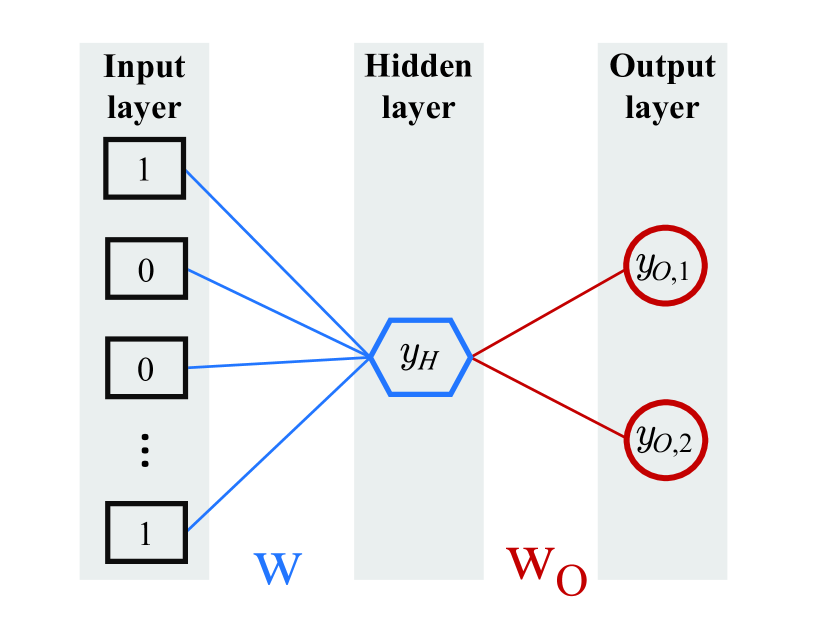
The shn-FNN consists of an input, hidden, and output layer, as illustrated in Fig. 1. The configuration is assigned to the input layer of shn-FNN by simply setting a -dimensional vector . The hidden layer contains one neuron that produces a one-dimensional vector . The output layer consists of two neurons that form a one-hot vector . These three layers are connected by two weight vectors and .
The activation function cosine is empirically chosen for the hidden layer so that
| (8) |
The vector in the output layer is determined by applying the softmax function, i.e.,
| (9) |
where the weight vector , is fixed. The function softmax executes normalization by an exponential function to obtain probabilities, which is usually used in classification tasks Goodfellow et al. (2016). Specifically, the function softmax gives two neurons and in the output layer, given by
| (10) |
In this work, we choose , so that and are distinguishable. Thus, the desired sign is determined as follows:
| (14) |
which equivalently indicates the sign of , i.e., in principle. Without one-hot representation, it has been proven that FNN performs worse since a categorization task turns into a regression task compulsively Goodfellow et al. (2016).
III Data sets and training
Data sets. We use the exact diagonalization (ED) method to obtain the ground-state wave function. In the wave function, the sign and the configuration for a specified basis constitute a sample in the data set . Each sign is encoded as a one-hot vector , , which can only take two valid combinations:
| (20) |
After arranging the samples in descending order of amplitude , we discard those with to avoid any artificial effects caused by the limited numeric precision. The remaining samples in the data set are divided into a training set and a testing set in a ratio Goodfellow et al. (2016). Thus, the number of samples in the testing set is given by .
Training. During the training scheme-, we employ the back-propagation (BP) algorithm Rumelhart et al. (1986) to optimize the variables in the weight vector while adaptively adjusting the learning rate using the Adam algorithm P and Ba (2014). The process aims to minimize the cross entropy, defined as
| (21) |
which sums over samples in the entire training set. Here, the one-hot vector , is the output of shn-FNN as the vector is input.
We employ the mini-batch method based on the stochastic gradient descent (SGD) Goodfellow et al. (2016); Wilson and Martinez (2003) to reduce the huge computational costs. Instead of using the entire training set directly, we randomly select samples to calculate the gradients of the weights at each training step. In such a case, Eq. (21) only sums over selected samples. This method performs well in accuracy and speed, and the random selection helps prevent the “over-fitting” problem. In our program, we implement shn-FNN and the Adam optimization using the ML library “TensorFlow” Abadi et al. (2016).
To evaluate the performance of shn-FNN, we introduce the accuracy rate (AR), which is calculated as the ratio of the number of successfully classified samples to the total number of samples in the data set , i.e., . To monitor the optimization process, we define two additional accuracy rates. At each training step, we calculate the number of samples successfully classified . Then, we evaluate the optimization by computing the accuracy rate . To provide a comprehensive evaluation, we utilize the testing set and define the accuracy rate , where represents the number of correctly classified samples in the testing set .
After each training step, we assess the convergence criterion , which measures the absolute value of the difference between the accuracy rates obtained in the current step and the previous step. We halt the training process once the convergent criterion falls below a threshold .
To exemplify how shn-FNN learns the sign rule, we study the ground state of a generalized Ising ring described by the Hamiltonian
| (22) |
where represents the strength of the coupling, and determines the orientation of the spin polarization.
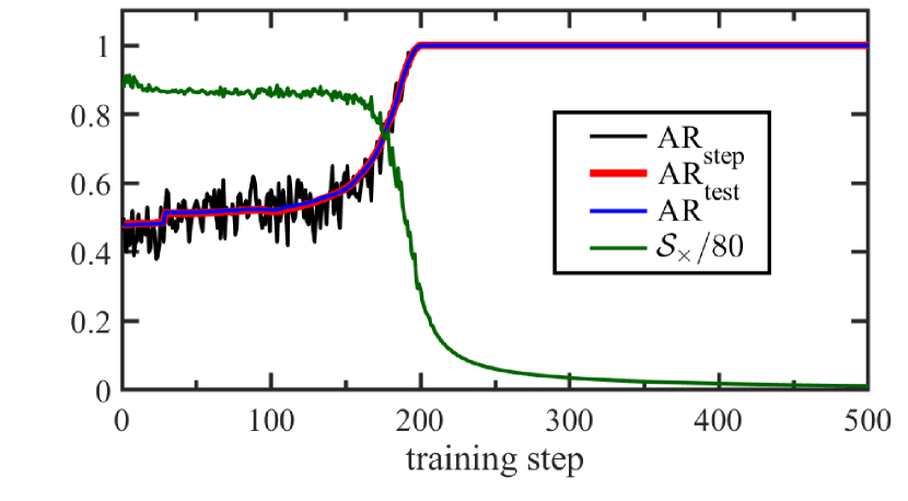
For the case of ferromagnetic coupling () and spin polarization along the x-axis (), we obtain the ground-state wave function for spins, and then prepare the data sets , and , as stated above. We initialize the weight vectors and in shn-FNN and start the training process. As illustrated in Fig. 2, the cross entropy rapidly decreases around the -th training step. After approximately training steps, the cross entropy tends towards stability, and the three accuracy rates , and AR consistently reach a maximum value or . We terminate the training process when the convergence criterion is met. In addition to scheme-, we will introduce scheme- in Sec. IV.2.1, tailored for frustrated spin models and the Fermi-Hubbard ring later.
IV Qubit lattice models
Using shn-FNN, we analyze the leading-order sign rules for various ordered ground states in qubit lattice models, including non-frustrated spin models in Sec. IV.1, frustrated spin models in Sec. IV.2, and interacting fermions in Sec. IV.3.
IV.1 Non-frustrated spin models
IV.1.1 A generalized ferromagnetic Ising ring
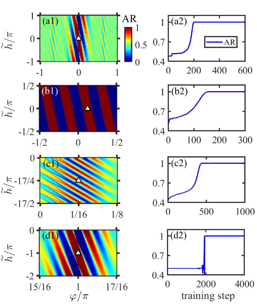
For the case of and in the model (22), the optimized shn-FNN with , as illustrated in Fig. 3(a.2), suggests that the weights in the sign rule (15). The physical interpretation of can be understood from the connection between Eq. (15) and the leading-order sign rule (7). Using Eq. (16), can be converted to a combination of the angles and the phase angle in the sign rule (7). This demonstrates the presence of ferromagnetic order along the x-axis, according to the spin-coherent state representation (2). To assume that in Eq. (16), we can visualize AR for the sign rule (15) in the (, ) plane, as shown in Fig. 3(a.1). The optimized weights are positioned at the coordinates of a maximum, i.e., and (black open triangle).
IV.1.2 A ferromagnetic spin- XY ring
For a spin- XY ring with sites, the Hamiltonian is given by
| (23) |
where represent the flipping-up and flipping-down operators for a spin-. The coupling strengths in the and -axes are equal in this ring.
For the case of shown in Fig. 3(b.2), the accuracy rate AR for shn-FNN reaches a perfect-classification limit of after approximately training steps. In the optimized shn-FNN, the weights are given by , which are equivalent to and according to Eq. (16). The result remains consistent with an in-plane ferromagnetic order, where all spins are confined to the xy-plane and aligned in the same polarization direction. Therefore, we still set in Eq. (16), and plot the AR distribution in the (, ) plane in Fig. 3(b.1). We can easily find that the weights correspond to the coordinates and (black open triangle). Since is uniform in space, the resulting sign rule (15) can be summarized as the Perron-Frobenius theorem Perron (1907); Frobenius (1909) by removing a global phase angle , when .
IV.1.3 A twisted ferromagnetic spin- XY ring
For a spin- XY ring with the ferromagnetic coupling strength under the twisted boundary condition (TBC), an antiferromagnetic bond connects site- and site- in the Hamiltonian
| (24) |
To achieve convergence of the accuracy rate , we train the shn-FNN for , as shown in Fig. 3(c.2). The optimized weights obtained from this training are given by
| (25) |
in the sign rule (15) for the ground-state wave function. We find Eq. (25) corresponds to a combination of the angles and the phase angle according to Eq. (16). This suggests a gradually varying spin profile in space with a pitch angle of . In a similar manner, by setting in Eq. (16), we parameterize the sign rule (15) with two parameters and . The AR distribution in the (, ) plane is plotted in Fig. 3(c.1), where the coordinates and are marked by a black open triangle.
The above result can be better understood through the following analysis. Under a rotation defined by the operators
| (26) |
the twisting effect from the antiferromagnetic bond is absorbed into a gauge field in a new Hamiltonian , where . Meanwhile,
| (27) |
Based on the arguement in App. A, it is found that the even-parity ground-state wave function for the Hamiltonian has positive signs, i.e., . As a result, the ground-state wave function for the Hamiltonian carries a nonzero complex phase factor due to the rotation . Specifically, it can be written as
| (28) |
Thus, the real part of the wave function is given by
| (29) |
which is inversion-symmetric concerning the chain center. It is worth noting that although Eq. (29) implies the same sign rule (15) obtained from the GWMF theory, this analysis is rigorous for the twisted spin- XY ring.
IV.1.4 An antiferromagnetic spin- XY ring
For the case of antiferromagnetic coupling , the optimized shn-FNN suggests in the sign rule (15), as shown in Fig. 3(d.1). We find that corresponds to a combination of the angles and the phase angle , indicating the presence of Nel order. Remarkably, the sign rule defined by is equivalent to MPR, where , and the quantity
| (30) |
sums over all odd sites. Here, we parameterize the sign rule (15) with two parameters and , by setting in Eq. (16). Fig. 3(d.1) illustrates the AR distribution in the (, ) plane, with the corresponding coordinates of the optimized represented by a black open triangle, specifically and . This sign rule is well understood because the ground-state wave function for is connected to the one for by a -rotation operation
| (31) |
Hence, it is evident that the sign rules in the XY ring with perfect AR, shown in Sec. IV.1.2, IV.1.3, and IV.1.4, adhere to a standardized format of weights Eq. (16) by setting with specific pitch angles , and . This pitch angle is related to the profile of spins rotating in space and can be acquired by training shn-FNN.
IV.1.5 An antiferromagnetic Heisenberg ring
In a pure antiferromagnetic Heisenberg ring (AFHR) with equal nearest-neighboring antiferromagnetic couplings in the , , and -axes, the spins at odd sites align anti-parallel to the spins at even sites according to GWMF. Even though the precise ground state behaves as the Tomonago-Luttinger liquid (TLL) Tomonaga (1950); Luttinger (1963); Haldane (1981), the optimized shn-FNN suggests MPR, which is consistent with previous studies Marshall (1955); Richter et al. (1994). We discuss the sign rule uniformly in the - AFHR in Sec. IV.2.1.
IV.2 Frustrated spin models
IV.2.1 A - antiferromagnetic Heisenberg ring
When the antiferromagnetic next-nearest-neighboring (NNN) Heisenberg coupling is introduced, we investigate the behavior of the frustrated spin- - AFHR. The Hamiltonian for this system is given by
| (32) |
where is a dimensionless ratio.
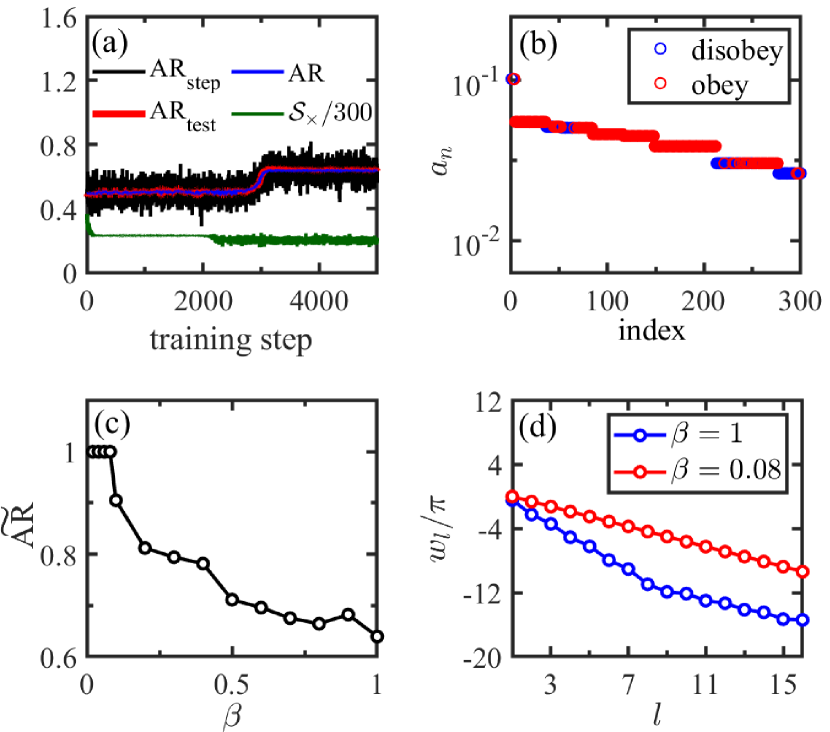
Using the techniques suggested in Sec. III and following training scheme- exemplified in Fig. 2, we initially train shn-FNN with all samples in the data set . For example, when the ratio , the optimization of shn-FNN searches for the minima of the cross entropy with extremely low efficiency. As illustrated in Fig. 4(a), three accuracy rates oscillate irregularly near the worst-performance limit of . After approximately training steps, all accuracy rates suddenly increase and reach another plateau. During this phase, the cross entropy exhibits random oscillation and fails to offer a meaningful gradient direction for updating the weight vector in shn-FNN. Once the accurate rate AR reaches approximately , the weight vector in the optimized shn-FNN (blue circles), as shown in Fig. 4(d), becomes difficult to interpret.
To address this issue, we sort samples in the descending order of amplitude , as shown in Fig. 4(b), and we observe that correct classification in the data set and wrong classification in the data set are irregularly mixed. Instead, we adopt training scheme-, where we use the first samples in the data set to train shn-FNN. In Fig. 4(c), as we reduce the selection rate , the accuracy rate approaches the perfect-classification limit of . With the optimized shn-FNN, out of samples are correctly classified. The resulting weight vector , shown in Fig. 4(d), exhibits a straight line in the sign rule (15), which will be used to demonstrate physical insight later.
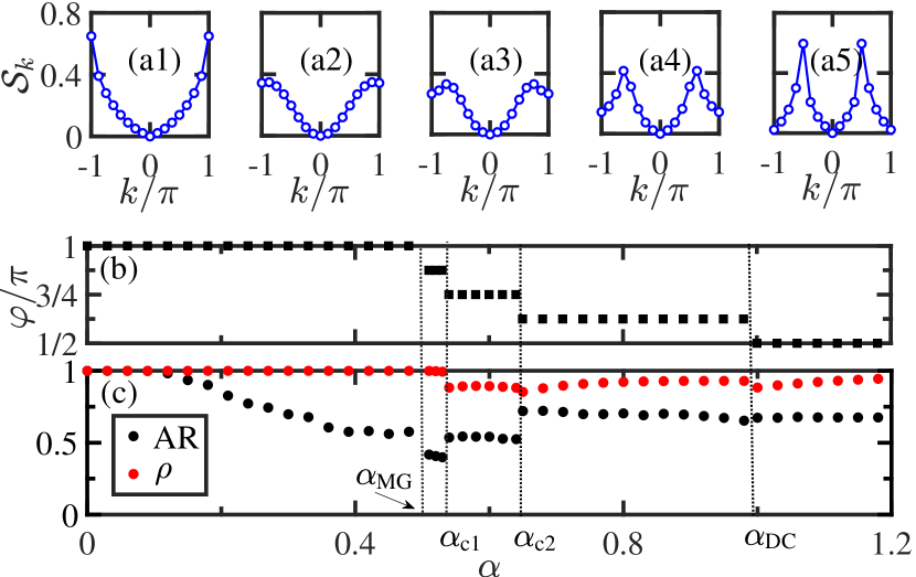
After conducting a systematical analysis of the ground states for sites, we have discovered that the optimized shn-FNN proposes the sign rules with weights Eq. (16) by setting , where the phase angle , as shown in Fig. 5(b). The integer number ranges from to , which allows us to divide the broad regime into five intervals. Within each interval, the value of plays the role of the commensurate/incommensurate pitch angle White and Affleck (1996); Soos et al. (2016). In Fig. 5(a.1-a.5), we observe that the double peaks in the structure factor
| (33) |
are located at the momenta . Due to the interplay of interactions, the accuracy rate and the correct weight
| (34) |
are shown in Fig. 5(c), where the data set includes samples obeying the leading-order sign rule (15). Besides, we find that the correct weight in the whole parameter regime is close to , which means that most of the samples with the largest amplitudes obey the leading-order sign rule, so the proposed scheme- works well.
The investigation of the sign rule provides consistent physical insights. At the Majumdar-Ghosh (MG) point , and for within the range , the leading-order sign rule is in accordance with MPR. As the ratio approaches infinity, one of the decoupled chains, composed of odd or even sites, individually follows MPR. However, away from that limit, a relatively tiny positive promotes a stable commensurate spin order with a pitch angle . When the ratio , commensurability is disrupted due to the emergence of triplet defects White and Affleck (1996); Soos et al. (2016). Between and , the ground state undergoes an incommensurate crossover White and Affleck (1996); Soos et al. (2016), which is indicated by the varying pitch angle in the weights of the leading-order sign rule (15), as shown in Fig. 5(b).
Besides, the ground state maintains the translation symmetry with a conserved momentum of either or , depending on the integer number , so that in the leading-order sign rule (7). Moreover, the center inversion symmetry of the chain imposes a constraint of . Consequently, in the equivalent sign rule (15), we choose the activation function sine/cosine for odd/even values of .
To quantitatively assess the violation of MPR when , we introduce a sign-fidelity
| (35) |
Here, we define the MPR state as
| (36) |
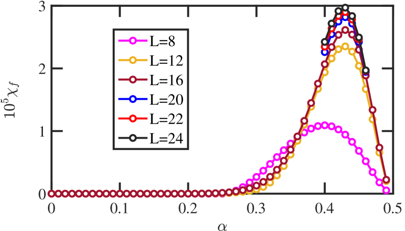
where the sign fully satisfies MPR. Thus, we get Retzlaff et al. (1993); Richter et al. (1994); Zeng and Parkinson (1995). In the vicinity of a continuous transition point, the minimum sign-fidelity or correct weight is expected to be achieved, indicating the most complicated sign rule Cai and Liu (2018); Westerhout et al. (2020). Like the orthogonalization catastrophe for free fermions Anderson (1967), fidelity follows a pow-law function of the system size . In principle, the relevant sign-fidelity susceptibility density, given by
| (37) |
is capable of identifying the places of continuous transition points Gu (2010). However, the maximum of is located at in the dimerized (DM) region Wang et al. (2009), where approaches a -independent function as shown in Fig. 6. It is possibly caused by the anomalous behavior of the exponential closure of gaps at the famous Berzinskii-Kosterlitz-Thouless (BKT) transition point Cincio et al. (2019).
IV.2.2 A spin- triangular XY antiferromagnet on a torus
Shn-FNN can learn the leading-order sign rules for the ground-state wave function of D quantum models, such as the XY model on triangular lattices with a size of sites, as shown in Fig. 7(a). The corresponding Hamiltonian for the model reads
| (38) |
and sums over all nearest-neighboring sites and . In the XC geometry, the lattice site labeled as , is identified by binary indices with , , and , , . The displacement for the site is given by .
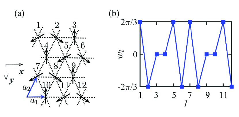
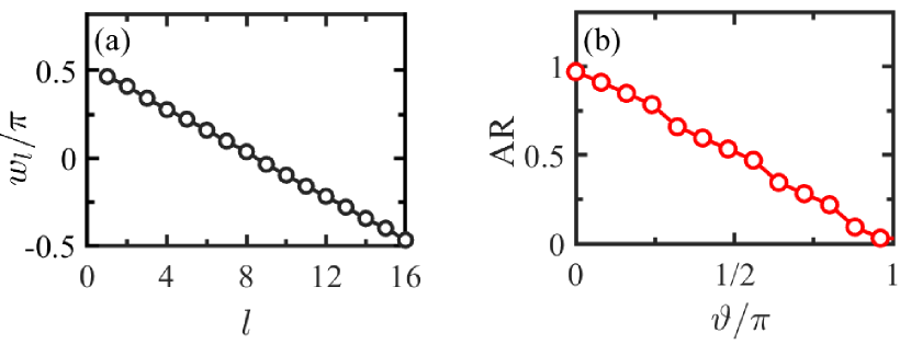
To ensure an exact hit at relevant high-symmetry momentum points in the first Brillouin zone, the length is chosen as a multiple of . Following training scheme-, the weights in the leading-order sign rule (15) are determined by the optimized shn-FNN. Specifically, we get
| (39) |
where if is even and otherwise, as illustrated in Fig. 7(b). This result matches the physical scenario of the coplanar order Bach et al. (2021) observed in previous studies, where the angle between spin polarization orientations at neighboring sites is always .
Moreover, the ground state possesses point group symmetries of the torus. These symmetry operations listed in table 1 carry eigenvalues of or , corresponding to the symmetric/even or antisymmetric/odd sector of the group representation in mathematics.
Let us discuss the mirror inversion about the y-axis. Under , the basis becomes but the sign is unchanged, so we have
| (40) |
For even , such as the lattice, the -symmetric ground-state wave function leads to in the leading-order sign rule (7), or equivalently the activation function cosine in Eq. (15), which obeys
| (41) |
In contrast, for odd , e.g., the geometry of lattices, the -antisymmetric ground-state wave function prefers in Eq. (7) and the sine function in Eq. (15). This difference is captured by shn-FNN in Fig. 8.
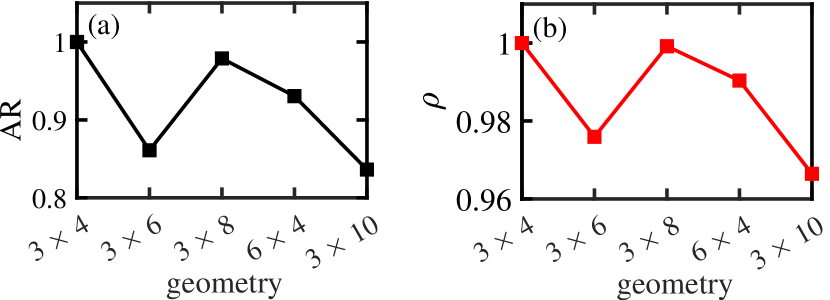
Furthermore, based on the mean-field picture of spinless Dirac fermions coupled to Chern-Simons gauge fields Wang et al. (2018); Sedrakyan et al. (2020), it has been shown that for different lattice geometries with finite and , non-condensed BCS pairs of spinons from high symmetry points would violate the leading-order sign rule, where both AR and deviate from . However, a more nuanced understanding of the subtle relationship between lattice geometry and the deviation from GWMF still needs to be included.
IV.3 A Fermi-Hubbard ring
The Fermi-Hubbard model is a simple model that describes the physics in strongly correlated electron systems, which is closely connected to quantum magnetism, metal-insulator transition, and the promising theory of high-temperature superconductivity Henderson et al. (1992); Essler et al. (2005); Moriya (2012). In a ring, the Hamiltonian for two-species fermions can be written as
| (42) |
where , and represent the creation, annihilation and particle number operators of fermion at site- respectively, , denotes the spin polarization, is the hopping amplitude between two nearest-neighboring sites, and is the onsite coulomb repulsion.
In the Fock space, each basis is a product of the bases for two species, that is,
| (43) |
Here, we define the vectors for species-. Under the conventional Jordan-Wigner transformation Derzhko (2001), the two-channel spin flipping operators can be represented by fermion operators as follows:
| (44) |
Thus, we get a two-leg spin- ladder
| (45) |
where
| (46) |
denote the transverse and longitudinal parts, respectively. The particle number operator in total for species- is given by . We are interested in the ground state for the case of , and even .
When , TBC is effectively applied to two decoupled chains in the spin-ladder model, as both and are even. For each species, when the parity of the ground state is even, the optimized shn-FNN with perfect AR can identify the leading-order sign rule given by
| (47) |
with the weights
| (48) |
depicted in Fig. 9(a). For the degenerate ground state with odd parity, the function cosine is replaced by the function sine, i.e.,
| (49) |
For small and any , the parity of the unique ground state is always even. In the case of , and , as illustrated in Fig. 9(b), the optimized shn-FNN suggests a sign rule
| (50) |
with the accuracy rate , where the vector is defined as
| (51) |
So, the resulting leading-order sign rule for the Fermi-Hubbard model remains consistent with the sign rule (15).
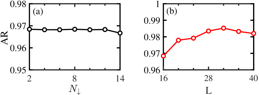
The leading-order sign rule (50) is robust and less dependent on the filling fraction and system size . In the case of and (Fig. 10), the accuracy rate AR is greater than for different . Additionally, as grows, the accuracy rate AR for gets closer to .
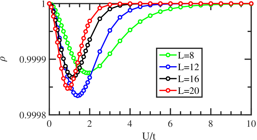
In the limit of large , only single occupations can exist in the ground state because of a considerable charge gap. As a result, spin fluctuations in the reduced Hilbert space of either spin-up or spin-down are described by the effective antiferromagnetic Heisenberg ring. The ground state for the effective model follows the MPR sign rule exactly. Returning to the fermion bases, it is easy to prove that the weights are the same as ones in the leading-order sign rule at . We can observe that the corresponding correct weight approaches when , as shown in Fig. 11.
According to the Bethe ansatz solution Lieb and Wu (1968), the Fermi liquid only survives at in the thermodynamical limit (TDL). However, because of a tiny charge gap close to , fermions exhibit behavior like a Fermi liquid in the ground state for system size limited to , much smaller than the correlation length. Consequently, a quasi-critical point is indicated by the minimum of the correct weight , where the strong quantum fluctuations would strongly violate the leading-order sign rules. As grows in Fig. 11, the quasi-critical point gradually approaches .
In an alternative definition of bases, that is,
| (52) |
the Jordan Wigner transformation changes accordingly, and an additional nonlinear appendix
| (53) |
exists in front of the predicted sign rules. However, this appendix can not be expressed in shn-FNN.
V Summary and discussions
We have successfully developed a Gutzwiller mean-field theory of sign rules for the ordered ground states in qubit lattice models, which perfectly matches the sign predicted by a shallow FNN with a single hidden neuron, called shn-FNN. By utilizing this principle, we provide a consistent explanation for the excellent performance of activation functions in the neural network and offer a vivid interpretation of the sign rule represented by FNN.
We systematically test our theory on various spin models and the Fermi-Hubbard ring. For non-frustrated spin- models, such as a generalized Ising ring, (twisted) XY rings, and an antiferromagnetic Heisenberg ring, the sign rules for ground states with magnetic orders can be fully captured by shn-FNN, where the accurate rate of the prediction can archive exactly. However, in the case of frustrated models where interactions compete, the complexity of sign rules for ground states is significantly enhanced, reducing prediction accuracy. Nonetheless, the leading-order sign rules obtained by optimizing shn-FNN still provide a visual scenario of orders in spins, with the characteristic weight vector closely related to pitch angles. In the Fermi-Hubbard ring, we can obtain a unified sign rule by selecting suitable bases.
GWMF may not be suitable for 1D models since quantum fluctuations tend to destroy long-range orders. However, our current work presents a fresh perspective by demonstrating that GWMF can effectively capture the leading-order sign rule in the wave function, where fluctuations in amplitudes are erased. Our theory is a simple starting point by removing short-range details in ordered states. It would be intriguing to explore the information encoded in high-order microscopic processes instead of focusing solely on the leading-order ones. Of course, the theory for general lattice models also deserves profound studies in the future.
VI Acknowlegement
We thank Tao Li, Rui Wang, Ji-Lu He, Wei Su, and Wei Pan for the grateful discussion. S. H. acknowledges funding from the Ministry of Science and Technology of China (Grant No. 2022YFA1402700) and the National Science Foundation of China (Grants No. 12174020). Z. P. Y. acknowledges funding from the National Science Foundation of China (Grants No. 12074041). S. H. and K. X. further acknowledge support from Grant NSAF-U2230402. The computations were performed on the Tianhe-2JK at the Beijing Computational Science Research Center (CSRC) and the high-performance computing cluster of Beijing Normal University in Zhuhai.
Appendix A Sign rule for the twisted ferromagnetic spin- XY rings
Here we prove that the even-parity ground-state wave function for the Hamiltonian with , mentioned in Sec. IV.1.3 of the main text, has positive signs .
Under the Jordan-Wigner transformation Derzhko (2001), the spin operators can be represented by fermion operators as follows:
| (54) |
where , , and represent the annihilation, creation, and particle number operators of fermion, respectively. As a result, the Hamiltonian can be transformed into the one for spinless free fermions defined as
| (55) |
The selection of periodic or twisted boundary conditions in the fermion model depends on whether the particle number is odd or even.
For odd , the single-particle levels are described by plane waves with discrete momenta , where the integer ranges from to . The energy for the -th single-particle level follows a formula with the phase angle . At half-filling , the ground state selects single-particle levels with the integer . Therefore, the ground-state wave function for the Hamiltonian , seen as a determinant of selected plane waves, is the same as the one for the other Hamiltonian at half-filling. Similarly, when is even, the ground-state wave function for the Hamiltonian is the same as the one for the Hamiltonian as well. In conclusion, both Hamiltonian for odd/even can be transformed back to the unique Hamiltonian through the inverse Jordan-Wigner transformation, where the even-parity ground-state wave function always has positive signs, according to the Perron-Frobenius theorem Perron (1907); Frobenius (1909).
References
- Eisert et al. (2010) J. Eisert, M. Cramer, and M. B. Plenio, Reviews of Modern Physics 82, 277 (2010).
- Chertkov and Clark (2018) E. Chertkov and B. K. Clark, Physical Review X 8, 031029 (2018).
- Wang et al. (2019) C. Wang, H. Zhai, and Y. Z. You, Science Bulletin 64, 1228 (2019).
- Irkhin and Skryabin (2019) V. Y. Irkhin and Y. N. Skryabin, Physics of Metals and Metallography 120, 513 (2019).
- Grover and Fisher (2015) T. Grover and M. P. A. Fisher, Physical Review A 92, 042308 (2015).
- Perron (1907) O. Perron, Mathematische Annalen 64, 248 (1907).
- Frobenius (1909) G. Frobenius, Matrices from positive elements. II, 1 (Walter de Gruyter & CO, Berlin, Germany, 1909) pp. 514–518.
- Marshall (1955) W. Marshall, Proceedings of the Royal Society of London. Series A. Mathematical and Physical Sciences 232, 48 (1955).
- Lieb et al. (1961) E. Lieb, T. Schultz, and D. Mattis, Annals of Physics 16, 407 (1961).
- Lieb and Mattis (1962) E. Lieb and D. Mattis, Journal of Mathematical Physics 3, 749 (1962).
- Zeng and Parkinson (1995) C. Zeng and J. B. Parkinson, Phys. Rev. B 51, 11609 (1995).
- Bursill et al. (1995) R. Bursill, G. A. Gehring, D. J. J. Farnell, J. B. Parkinson, T. Xiang, and C. Zeng, Journal of Physics: Condensed Matter 7, 8605 (1995).
- Retzlaff et al. (1993) K. Retzlaff, J. Richter, and N. B. Ivanov, Zeitschrift für Physik B Condensed Matter 93, 21 (1993).
- Richter et al. (1994) J. Richter, N. B. Ivanov, and K. Retzlaff, Europhysics Letters 25, 545 (1994).
- Cai and Liu (2018) Z. Cai and J. Liu, Phys. Rev. B 97, 035116 (2018).
- Westerhout et al. (2020) T. Westerhout, N. Astrakhantsev, K. S. Tikhonov, M. I. Katsnelson, and A. A. Bagrov, Nature Communications 11, 1593 (2020).
- White (1992) S. R. White, Physical Review Letters 69, 2863 (1992).
- Peschel et al. (1999) I. Peschel, M. Kaulke, X. Wang, and K. Hallberg, eds., Density-Matrix Renormalization (Springer Berlin Heidelberg, 1999).
- Schollwöck (2011) U. Schollwöck, Annals of Physics 326, 96 (2011).
- Orús (2014) R. Orús, Annals of Physics 349, 117 (2014).
- Carleo and Troyer (2017) G. Carleo and M. Troyer, Science 355, 602 (2017).
- Carleo et al. (2019) G. Carleo, I. Cirac, K. Cranmer, L. Daudet, M. Schuld, N. Tishby, L. Vogt-Maranto, and L. Zdeborová, Reviews of Modern Physics 91, 045002 (2019).
- Jia et al. (2019) Z. A. Jia, B. Yi, R. Zhai, Y. C. Wu, G. C. Guo, and G. P. Guo, Advanced Quantum Technologies 2, 1800077 (2019).
- Vivas et al. (2022) D. R. Vivas, J. Madroñero, V. Bucheli, L. O. Gómez, and J. H. Reina, arXiv preprint arXiv:2204.12966 (2022).
- Choo et al. (2019) K. Choo, T. Neupert, and G. Carleo, Physical Review B 100, 125124 (2019).
- Szabó and Castelnovo (2020) A. Szabó and C. Castelnovo, Physical Review Research 2, 033075 (2020).
- Bukov et al. (2021) M. Bukov, M. Schmitt, and M. Dupont, SciPost Physics 10, 147 (2021).
- Roscher et al. (2020) R. Roscher, B. Bohn, M. F. Duarte, and J. Garcke, IEEE Access 8, 42200 (2020).
- He et al. (2020) C. He, M. Ma, and P. Wang, Neurocomputing 387, 346 (2020).
- Fan et al. (2021) F. L. Fan, J. J. Xiong, M. Z. Li, and G. Wang, IEEE Transactions on Radiation and Plasma Medical Sciences 5, 741 (2021).
- Raissi et al. (2019) M. Raissi, P. Perdikaris, and G. Karniadakis, Journal of Computational Physics 378, 686 (2019).
- Yuan and Weng (2021) J. Yuan and Y. Weng, in 2021 IEEE International Conference on Data Mining (ICDM) (IEEE, 2021).
- Cai et al. (2021) S. Cai, Z. Mao, Z. Wang, M. Yin, and G. E. Karniadakis, Acta Mechanica Sinica 37, 1727 (2021).
- Vasiliev et al. (2018) A. Vasiliev, O. Volkova, E. Zvereva, and M. Markina, npj Quantum Materials 3, 18 (2018).
- Gardiner and Zoller (2017) C. Gardiner and P. Zoller, The Quantum World of Ultra-Cold Atoms and Light Book III: Ultra-Cold Atoms (World Scientific (Europe), 2017).
- Meher and Sivakumar (2022) N. Meher and S. Sivakumar, arXiv:2204.01322 (2022).
- Makhlin et al. (2001) Y. Makhlin, G. Schön, and A. Shnirman, Review Modern Physics 73, 357 (2001).
- Luo (2008) S. L. Luo, Physics Review A 77, 042303 (2008).
- Kjaergaard et al. (2020) M. Kjaergaard, M. E. Schwartz, J. Braumüller, P. Krantz, J. I.-J. Wang, S. Gustavsson, and W. D. Oliver, Annual Review of Condensed Matter Physics 11, 369 (2020).
- Penc and Läuchli (2010) K. Penc and A. M. Läuchli, in Introduction to Frustrated Magnetism (Springer Berlin Heidelberg, 2010) pp. 331–362.
- Gutzwiller (1963) M. C. Gutzwiller, Physical Review Letters 10, 159 (1963).
- Gutzwiller (1965) M. C. Gutzwiller, Physical Review 137, A1726 (1965).
- Cybenko (1989) G. Cybenko, Mathematics of Control, Signals and Systems 2, 303 (1989).
- Hornik et al. (1989) K. Hornik, M. Stinchcombe, and H. White, Neural Networks 2, 359 (1989).
- Goodfellow et al. (2016) I. Goodfellow, Y. Bengio, and A. Courville, Deep Learning (MIT Press, 2016) http://www.deeplearningbook.org.
- Iten et al. (2020) R. Iten, T. Metger, H. Wilming, L. del Rio, and R. Renner, Physical Review Letters 124, 010508 (2020).
- Wang et al. (2021) W. Wang, Z. Wang, Y. Zhang, B. Sun, and K. Xia, Physical Review Applied 16, 014005 (2021).
- Rumelhart et al. (1986) D. E. Rumelhart, G. E. Hinton, and R. J. Williams, in Parallel Distributed Processing, edited by D. E. Rumelhart and R. J. McClelland (MIT Press, Cambridge, Mass., 1986) Chap. 8.
- P and Ba (2014) D. P, Kingma and J. Ba, arxiv:1412.6980 (2014).
- Wilson and Martinez (2003) D. Wilson and T. R. Martinez, Neural Networks 16, 1429 (2003).
- Abadi et al. (2016) M. Abadi, P. Barham, J. Chen, Z. Chen, A. Davis, J. Dean, M. Devin, S. Ghemawat, G. Irving, M. Isard, M. Kudlur, J. Levenberg, R. Monga, S. Moore, D. G. Murray, B. Steiner, P. Tucker, V. Vasudevan, P. Warden, M. Wicke, Y. Yu, and X. Zheng, in 12th USENIX Symposium on Operating Systems Design and Implementation (OSDI 16) (USENIX Association, Savannah, GA, 2016) pp. 265–283.
- Tomonaga (1950) S. I. Tomonaga, Progress of Theoretical Physics 5, 544 (1950).
- Luttinger (1963) J. M. Luttinger, Journal of Mathematical Physics 4, 1154 (1963).
- Haldane (1981) F. D. M. Haldane, Journal of Physics C: Solid State Physics 14, 2585 (1981).
- White and Affleck (1996) S. R. White and I. Affleck, Physical Review B 54, 9862 (1996).
- Soos et al. (2016) Z. G. Soos, A. Parvej, and M. Kumar, Journal of Physics: Condensed Matter 28, 175603 (2016).
- Anderson (1967) P. W. Anderson, Physical Review Letters 18, 1049 (1967).
- Gu (2010) S. J. Gu, International Journal of Modern Physics B 24, 4371 (2010).
- Wang et al. (2009) L. Wang, S.-J. Gu, and S. Chen, arXiv:0903.4242 (2009).
- Cincio et al. (2019) L. Cincio, M. M. Rams, J. Dziarmaga, and W. H. Zurek, Physical Review B 100, 081108(R) (2019).
- Bach et al. (2021) A. Bach, M. Cicalese, L. Kreutz, and G. Orlando, Calculus of Variations and Partial Differential Equations 60, 149 (2021).
- Wang et al. (2018) R. Wang, B. Wang, and T. A. Sedrakyan, Physical Review B 98, 064402 (2018).
- Sedrakyan et al. (2020) T. Sedrakyan, R. Moessner, and A. Kamenev, Physical Review B 102, 024430 (2020).
- Henderson et al. (1992) J. A. Henderson, J. Oitmaa, and M. C. B. Ashley, Phys. Rev. B 46, 6328 (1992).
- Essler et al. (2005) F. H. Essler, H. Frahm, F. Göhmann, A. Klümper, and V. E. Korepin, The one-dimensional Hubbard model (Cambridge University Press, 2005).
- Moriya (2012) T. Moriya, Electron Correlation and Magnetism in Narrow-Band Systems: Proceedings of the Third Taniguchi International Symposium, Mount Fuji, Japan, November 1–5, 1980, Vol. 29 (Springer Science & Business Media, 2012).
- Derzhko (2001) O. Derzhko, arXiv:cond-mat/0101188 (2001).
- Lieb and Wu (1968) E. H. Lieb and F. Y. Wu, Physical Review Letters 20, 1445 (1968).