RDFNet: Regional Dynamic FISTA-Net for Spectral
Snapshot Compressive Imaging

Abstract

Deep convolutional neural networks have recently shown promising results in compressive spectral reconstruction. Previous methods, however, usually adopt a single mapping function for sparse representation. Considering that different regions have distinct characteristics, it is desirable to apply various mapping functions to adjust different regions’ transformations dynamically. With this in mind, we first introduce a regional dynamic way of using Fast Iterative Shrinkage-Thresholding Algorithm (FISTA) to exploit regional characteristics and derive dynamic sparse representations. Then, we propose to unfold the process into a hierarchical dynamic deep network, dubbed RDFNet. The network comprises multiple regional dynamic blocks and corresponding pixel-wise adaptive soft-thresholding modules, respectively in charge of region-based dynamic mapping and pixel-wise soft-thresholding selection. The regional dynamic block guides the network to adjust the transformation domain for different regions. Equipped with the adaptive soft-thresholding, our proposed regional dynamic architecture can also learn appropriate shrinkage scale in a pixel-wise manner. Extensive experiments on both simulated and real data demonstrate that our method outperforms prior state-of-the-arts. Our code and data are available at https://github.com/SherryZhou97/RDFNet.

I Introduction

Hyperspectral image contains large amount of spatial information across a multitude of wavelengths, which makes it enjoy the great potential of wide applications, such as remote sensing [1], medical diagnosis [2], biomedical engineering [3], archaeology and art conservation [4], food inspection [5] and environmental monitoring [6].

However, capturing hyperspectral images poses a great challenge since each wavelength needs to be captured separately, which is time consuming and limits the practicality of this technique. Traditional methods of spectral imaging include whiskbroom scanning [7], pushbroom scanning [8], and wavelength scanning [9]. Such scanning methods suffer a long spectral image acquisition process, making them inapplicable for large scenes or dynamic recording. To mitigate this, researchers start to explore snapshot spectral imaging [10]. Early endeavors include integral field spectrometry, multispectral beam splitting, and image-replicating imaging spectrometer [11]. These methods, though achieve multispectral imaging through splitting light [12][13], still fail to obtain massive spectral channels and require bulky optical systems.

Figure 1: Motivation of this work. (a) The characteristics, i.e., sparsity and flatness, vary significantly across four regions randomly selected from a real hyperspectral measurement. (b) Conventional global static transformation. (c) Our proposed regional dynamic transformation.

To tackle the above problems, snapshot compressive imaging (SCI) equipped with advanced compressive sensing (CS) [14, 15] algorithms has received growing attention due to its elegant combination of optics, mathematics, and optimization theory [12]. Among typical SCI systems, the passive modulation coded aperture snapshot spectral imaging (CASSI) system, which uses a single disperser coded aperture compressive spectral image [16, 17], stands out due to its low power consumption. It uses a coded aperture to block or filter the input light field, which serves as the encoding process in compressive sensing pipeline [12]. This process plays a role in information compression, which is flexible in design and provides the prior knowledge for subsequent reconstruction. Different from hardware based encoding, its decoding process largely relies on the computation via designed algorithms. Hence the core challenge of CASSI is to efficiently reconstruct the underlying 3D spectral image from under-sampled 2D measurement.

Traditional reconstruction methods are iterative [18][19][20] and require the designed measurement of the encoding process and other prior knowledge for reconstruction. As a result, the decoding process is computationally expensive and takes minutes or even hours for spectral reconstruction. Moreover, the degradation issue when using limited measurements also hinders the application under resource constrained conditions. To recover the spectra modeled in the complex diffraction process, the powerful deep learning technique is required.

With the rise of Deep Neural Networks (DNN), many studies have attempted to combine DNN with traditional optimization process to replace iterative optimization [21, 22, 23, 24]. Pioneering works [25, 26] tackle this problem by learning a static sparse transformation for the entire image and by using a fixed threshold to obtain the closed-form solution. Nevertheless, we found that different regions of an image have dramatically distinct characteristics. As illustrated in Fig. 1, the sparsity (measured by $l_{1}$-norm) and the flatness (measured by average gradient) vary significantly across different regions in real hyperspectral measurement. Inspired by this, we argue that regarding the entire image as a whole and using a single global mapping function may limit the representation of sparse transformation. Different regions need to be transformed into varying sparse domains using different mapping functions based on their unique regional characteristics. In addition, the soft-thresholding is used to effectively shrinkage and eliminate the noise-related features in a sparse transformation domain. Similarly, we can dynamically determine the shrinkage scale depending on regions’ features. There is much redundancy between high-dimensional information and simple signals in conventional FISTA, a fixed threshold may also limit the denoising capability of the transformation network.

In light of above, this work gives a novel region-based dynamic FISTA [27] algorithm that uses a regional feature guided weighting approach to dynamically derive the solution in sparse transformation. Guided by the algorithm, we further present a newly designed hierarchical dynamic architecture, dubbed RDFNet, that adopts dynamical multiple mapping functions and uses an efficient and effective strategy to dynamically select the appropriate soft-thresholding of transformation.

Specifically, RDFNet uses multiple transformation blocks implemented by multilayer perception (MLP) to learn distinct sparse representations. Each of the blocks strictly corresponds to one specific sparse domain. Instead of using a fixed threshold, we design a new adaptive soft-thresholding module to automatically determine the threshold, such that the proposed dynamic FISTA transformation block is capable of learning a more appropriate shrinkage scale in each sparse domain. Then, we utilize a regional dynamic sub-network to extract the regions’ characteristics and generate transform domain weights for each block. After that, RDFNet constructs its sparse representation by dynamically assembling multiple fundamental FISTA transformations with regional feature-guided scoring weights. Hence sparse representations are aggregated dynamically for each region. As a result, our regional dynamic mechanism can greatly enhance the transformation capability of the reconstruction model.

Extensive experiments demonstrate that the proposed RDFNet outperforms other reconstruction methods on multiple simulation datasets including KAIST [28], CAVE [29] and ICVL [30], and also achieves competitive performance on real datasets. In particular, our RDFNet achieves state-of-the-art performance of $33.34$dB in average PSNR and $0.956$ in average SSIM on $10$ scenes of KAIST [28]. For the natural image dataset ICVL [30], our method achieves an average PSNR of 35.51dB. It also surpasses the previously best-performing DNU by a large margin of $2.9$dB in average PSNR on ICVL [30] comprised of natural images.

Moreover, our RDFNet is lightweight with only $1.29$M parameters and runs at a fast inference speed of $0.11$ second per image. These results clearly demonstrate the superiority of RDFNet over prior state-of-the-arts in terms of both accuracy and efficiency.

To sum up, this work makes the following contributions:

• We propose a new regional dynamic FISTA algorithm for coded aperture snapshot spectral imaging and design a novel hierarchical dynamic architecture RDFNet.

• We present a learnable pixel-wise adaptive soft-thresholding module to automatically determine the shrinkage scale in each transformation block.

• We establish new state-of-the-arts on three popular simulation datasets and a real dataset.

II Related Work

II-A Dynamic Mechanism

Our work is related to the recent dynamic mechanism. In particular, Chen et al. [31] propose a dynamic convolution that aggregates multiple convolution kernels dynamically based on the input. Brabandere et al. [32] present a dynamic filter network to dynamically generate position-specific filters on pixel inputs. CondConv [33] generates convolution kernels by combining several filters through a routing function. Recently, PAConv [34] develop a position adaptive convolution operator with dynamic kernel assembling for point cloud processing. However, the region-based dynamic mechanism has not yet been explored in the field of SCI reconstruction. Zhang et al. [35] design a weight for each pixel in an image, use the same transformation to perform super-resolution, and add the weights to obtain a mixed transformation for the entire image. In comparison, we split the image into regions instead of pixels and perform distinct domain transformations with pixel-level adaptive thresholding for different regions while retaining neighborhood information.

II-B Learning based Deep Image Prior(DIP)

With the rise of neural networks, some algorithms try to use the convolution to obtain the DIP but there is no deep network structure, forming a machine learning algorithm.

Bacca J. et al [36] proposed a network for spectral reconstruction without training according to the ideas of solving ill-posed problems with low rank. It is mainly achieved by analyzing the low-rankness of images at the first layer of the network. Evaluating the difference between minimized compression measurements and predictions by the use of $l_{2}$. However, it does not really use a deep neural network in the process of solving, but uses several convolutions to help getting the prior of recon. Van Veen D. et al [37] also proposed an untrained model, which may belong to a kind of machine learning method. The neural network is only used to learn the weight of the prior information, not the way to really obtain the prior information, and the neural network here is not deep, but only uses the volume product. Inspired by the linear mixture model (LMM) for spectral image, Gelvez T. et al [38] decomposed the image into a matrix, and uses the neural network to learn the weights and features of each matrix as the depth prior of the image for reconstruction.

In [39], DIP is employed as a refinement process of the trained network for the reconstruction of a single image. The other related work is DeepRED [40], where DIP is combined with Regularization by Denoising (RED) [41]. And the hyperspectral way of using deepred [40] is [42]. In fact, most of the processes have nothing to do with the design of deep neural networks, and does not using the characteristics of adjusting the transformation domain for optimizing reconstruction tasks.

II-C Deep Learning-based Algorithms

Inspired by the prevalence of deep learning in the field of high-level visions, some researchers have attempted to use deep convolution neural networks (CNNs) to learn the inverse process. These deep learning-based algorithms can be divided into three streams: End-to-End (E2E) [43, 24, 44, 22], Plug-and-Play (PNP) [45, 46, 21], and deep unfolding [47, 26, 48, 23, 49].

End-to-End(E2E): E2E-CNNs first applied for its great migration. Both the U-net [43] and GAN [44] structure has been used for video SCI. The self attention mechanism has been attempted in TSA-Net [22] for spectral SCI. The $\lambda$-Net [24], where a two stage network was proposed. E2E-CNNs enjoy the advantage of fast inference after training, however, it requires a large amount of training data and excessive training time. In addition, E2E-CNN lacks flexibility as well as interpretability.

Plug-and-Play(PNP): The PnP based algorithms employ pre-trained deep denoising networks as priors and integrate them into the iterative algorithms. Now, applying the well pre-trained denoising networks, such as the FFDNet [50], with ADMM or GAP into SCI leads to fast, flexible and efficient algorithms. The PNP-ADMM [45] and PNP-GAP [47] have recently been developed into flexible deep denoisers. A joint reconstruction and demosaicing framework has recently been proposed in [51] for video SCI and a deep denoiser in [21] has shown competitive performance for spectral SCI. However, the pre-trained networks in PnP methods are fixed without re-training, therefore limiting the performance.

Deep Unfolding: Deep unfolding merges the advantages of the iterative optimization and E2E-CNNS by training a concatenation of small CNNs to simulate the iterative operations in traditional optimization, where each phase is referred to as a stage. Optimization-based update rules are used to connect these phases and train in an end-to-end fashion. It is somewhat interpretable. Since the small CNNs are independent of the sensing matrix, they can be trained with a smaller dimension than the size of the desired signal, which makes them both training and testing faster than E2E-CNN.

Most recently, the GAP-net proposed in [47] has achieved good results in both video and spectral SCI. A deep unfolding based on the Gaussian scale mixture model has been developed in [48] for spectral SCI reconstruction. DNU [23] has contributed to the introduction of a new prior for optimization. Zhang and Wang [49] first learned the tensor low-rank prior of hyperspectral images in the feature domain by DNN to promote the reconstruction quality.

Nonetheless, these methods still show limitations in modeling sparsity representations. Besides, the guidance of regional characteristics for adjusting the reconstruction transformation domain is under-studied.

III Method

We first revisit the typical CASSI observation model, then introduce our regional dynamic FISTA algorithm, and finally elaborate our regional dynamic FISTA network (RDFNet).

Figure 2: Schematic diagrams of spectral snapshot compressive imaging, a.k.a., coded aperture snapshot spectral imaging (CASSI) system. The spatial-spectral datacube is first modulated by a fixed physical mask and then the modulated datacube is sheared by a disperser. The 2D coded measurement thus includes the information of the spectral datacube, which is the desired 3D signal.

III-A CASSI Observation Model

Spectral snapshot compressive imaging (SCI) sysmtem comprises of a hardware encoder and a software decoder. The encoder denotes the optical system that compresses 3D data cube $(x,y,\lambda)$ to a snapshot measurement on a 2D detector. The decoder denotes the reconstruction algorithm used to recover the 3D data cube from the snapshot measurement. Here, we focus on the coded aperture snapshot spectral imaging (CASSI) system that uses a fixed mask and a disperser to implement band-wise modulation.

As shown in Fig.2, each spatial position of the scene is modulated by a coded aperture (mask) that blocks or unblocks the incoming light. Then the coded spectral scene passes through the prism to introduce a horizontal shifting. Finally, the coded shifted spectral scene is integrated along the spectral axis by the detector, resulting in 2D compressed measurement.

Following the theory in [52], let $X\in\mathbb{R}^{N_{x}\times N_{y}\times N_{\lambda}}$ denote the 3D spatial-spectral cube and $M^{0}\in(0,1)^{N_{x}\times N_{y}}$ the physical mask used for signal modulation. We use $X^{\prime}\in\mathbb{R}^{N_{x}\times N_{y}\times N_{\lambda}}$ to represent the modulated signal where images at different wavelengths are modulated separately by the same mask. For $n_{\lambda}\in\left\{1,....,N_{\lambda}\right\}$, we have:

$$X^{\prime}(:,:,n_{\lambda})=X(:,:,n_{\lambda})\odot M^{0},$$ (1)

where $\odot$ represents element-wise multiplication.

Next comes the disperser, which disperses the light to different spatial locations based on their wavelengths. After the modulated cube passes the disperser, $X^{\prime}$ is tilted and considered to be sheared along the $y-$axis. We use $X^{\prime\prime}\in\mathbb{R}^{N_{x}\times(N_{y}+N_{\lambda}-1)\times N_{\lambda}}$ to denote the tilted cube and assume $\lambda_{c}$ to be the reference wavelength. That is, image $X^{\prime}(:,:,n_{\lambda_{c}})$ is not sheared along the $y-$axis, we hence have:

$$X^{\prime\prime}(u,v,n_{\lambda})=X^{\prime}(x,y+d(\lambda_{n}-\lambda_{c}),n_{\lambda}),$$ (2)

where $(u,v)$ indicates the coordinate system on the detector plane, and $\lambda_{n}$ is the wavelength of channel $n_{\lambda}$. Here, $d(\lambda_{n}-\lambda_{c})$ signifies the spatial shifting for channel $n_{\lambda}$. The compressed measurement at the detector $y(u,v)$ can thus be modeled as

$$y(u,v)=\int_{\lambda_{m}in}^{\lambda_{m}ax}x^{\prime\prime}(u,v,n_{\lambda})d\lambda,$$ (3)

since the sensor integrates all the light in the wavelength range $[\lambda_{min},\lambda_{max}]$, where $f^{\prime\prime}$ is the continuous representation of $F^{\prime\prime}$. In discretized form, the captured 2D measurement $Y\in\mathbb{R}^{N_{x}\times(N_{y}+N_{\lambda}-1)}$ is

$$Y=\sum_{n_{\lambda}=1}^{N_{\lambda}}X^{\prime\prime}(:,:,n_{\lambda})+\epsilon,$$ (4)

which is a compressed frame containing information of all the modulated spectral channels and $\epsilon\in\mathbb{R}^{N_{x}\times(N_{y}+N_{\lambda}-1)}$ represents the measurement noise. For simplicity purpose, we denote $M\in R^{N_{x}\times(N_{y}+N_{\lambda}-1)\times N_{\lambda}}$ as the shifted version of the physical mask corresponding to different wavelengths,

$$M(u,v,n_{\lambda})=M^{0}(x,y+d(\lambda_{n}-\lambda_{c})).$$ (5)

Similarly, for each signal frame at different wavelengths, the shifted version $\tilde{X}\in R^{N_{x}\times(N_{y}+N_{\lambda}-1)\times N_{\lambda}}$ is

$$\tilde{X}(u,v,n_{\lambda})=X(x,y+d(\lambda_{n}-\lambda_{c}),n_{\lambda}).$$ (6)

Based on the above, measurement $Y$ can be represented as

$$Y=\sum_{n_{\lambda}=1}^{N_{\lambda}}\tilde{X}(:,:,n_{\lambda})\odot M(:,:,n_{\lambda})+\epsilon.$$ (7)

This corresponds to the encoding process of SCI in Fig.2. Note that the 3D mask $M$ can be obtained by calibration. Given the solved $\tilde{X}$, we can obtain the desired 3D cube by shifting it back to $F$ based on the relationship in Eq.(6),

$$x=[x_{1}^{T},...,x_{N_{t}}^{T}]^{T},\Phi=[D_{1},...,D_{N_{t}}]^{T},$$ (8)

where $x_{k}=vec(X_{k})$ represents the vectorization of frame $k$ and $D_{k}=Diag(vec(M_{k}))$ is a diagonal matrix with diagonal elements vectorized of $M_{k}$. We obtain the forward model

$$\bm{y}=\bm{\Phi x}+\epsilon,$$ (9)

which is the core problem of spectral SCI reconstruction. Conventional methods [53, 54, 55] usually employ a regularization term $R(\bm{x})$ as prior to constrain the solution in desired signal space. These algorithms aim to find an estimated $\bm{\bar{x}}$ of $\bm{x}$ by solving the following problem:

$$\bm{\bar{x}}=\arg\min_{\bm{x}}\frac{1}{2}||\bm{y}-\bm{\Phi x}||_{2}^{2}+\lambda R(\bm{x}),$$ (10)

where $\lambda$ is a parameter to balance between the fidelity and the regularization term. Eq.(10) is usually solved by iterative algorithms with various image priors of $R(\bm{x})$ including sparsity [53], total variation [54], deep denoising prior [45, 21], autoencoder prior[43], etc.

III-B Regional Dynamic FISTA Algorithm

Given the measurement $\bm{y}$ and the modulate mask $\bm{\Phi}$, the problem of reconstructing hyperspectral image $\bm{x}$ can be solved by LASSO optimization [56]. Using $l_{1}$-norm to impose sparsity constraint for coefficients [25], the reconstruction problem in Eq.(10) can be converted as

$$\bm{\bar{x}}=\arg\min_{x}\frac{1}{2}||\bm{y}-\bm{\Phi x}||_{2}^{2}+\lambda||\bm{\Psi x}||_{1},$$ (11)

where $\bm{\Psi x}$ denotes the coefficients in the transformation domain. By introducing an auxiliary parameter $\bm{r}^{k}$, the unconstrained optimization in Eq.(11) can be solved by iterative steps [27]:

$$\bm{x}_{k}=\arg\min_{x}\frac{1}{2}||\bm{x}-\bm{r}^{k}||_{2}^{2}+\lambda||\bm{\Psi x}||_{1},$$ (12)

$$\bm{r}^{k}=\bm{z}^{k}-\rho\bm{\Phi}(\bm{\Phi z}^{k}-\bm{y}),$$ (13)

$$t^{k+1}=\frac{1+\sqrt{1+4(t^{k})^{2}}}{2},$$ (14)

$$\bm{z}^{k+1}=\bm{x}^{k}+(\frac{t^{k}-1}{t^{k}+1})(\bm{x}^{k}-\bm{x}^{k-1}),$$ (15)

where $k\geq 1$, $\bm{z}^{1}=\bm{x}^{0},t^{1}=1$, $\rho$ represents the step size. $\bm{z}^{k+1}$ is a new strating point for next iteration. In each step, we directly utilize the updated $t^{k}$ to calculate $\bm{z}^{k}$.

Figure 3: Overall architecture of RDFNet. The upper part demonstrates the data flow in RDFNet, containing K phases. The bottom part is the detailed network implementation of a phase, including pretreatment, dynamic FISTA blocks equipped with pixel-wise adaptive soft-thresholding module, and a sub-network for regional dynamic aggregation.

Conventional FISTA algorithm [27] regards the image as a whole and performs simple global static transformation using a single mapping function. However, we found that there exist significant differences among different regions in a measurement. Hence we are dedicated to applying distinct mapping functions for different regions based on their unique characteristics to realize region-adaptive transformation.

Based on the tensorlization operations [25], we re-reference the theoretical process of RDFNet to match our regional dynamic transformation and pixel-wise soft-thresholding. Specifically, we divide input $\bm{r}^{k}$ into a series of regions $\bm{r}_{i}^{k}\in\left\{\bm{r}_{1}^{k},...,\bm{r}_{M}^{k}\right\}$, and process each individual region using a dynamic mapping function determined by the region’s characteristics. By using $F(\cdot)$ to learn the sparsest representation of spectral images, we can obtain the regional results $\bm{x}_{i}^{k}\in\left\{\bm{x}_{1}^{k},...,\bm{x}_{M}^{k}\right\}$ based on the relationship in Eq.(11):

$$\bm{x}_{i}^{k}=\arg\min_{\bm{x}_{i}^{k}}\frac{1}{2}||\bm{x}_{i}^{k}-\bm{r}_{i}^{k}||_{2}^{2}+\lambda||F(\bm{x}_{i}^{k})||_{1}.$$ (16)

Following the Parseval Theorem

$$||\bm{Da}-\bm{Db}||_{2}=||\bm{a}-\bm{b}||_{2},$$ (17)

where $\bm{D}$ is an orthonormal transformation matrix. Eq.(16) can be converted as

$$\bm{x}_{i}^{k}=\arg\min_{\bm{x}_{i}^{k}}\frac{1}{2}||F(\bm{x}_{i}^{k})-F(\bm{r}_{i}^{k})||_{2}^{2}+\lambda||F(\bm{x}_{i}^{k})||_{1}.$$ (18)

According to the soft-thresholding theory [57], we adopt soft-thresholding operator to obtain the closed-form solution for each region:

$$\bm{x}_{i}^{k}=\hat{F}^{\prime}(soft(\hat{F}(\bm{r}_{i}^{k}),\lambda)),$$ (19)

where $\hat{F}^{\prime},\hat{F}$ are the mixture dynamic transformation. By summing up the regional results $\bm{x}_{i}^{k}\in\left\{\bm{x}_{1}^{k},...,\bm{x}_{M}^{k}\right\}$, we can obtain the final solution $\bm{x}^{k}$.

To achieve the adjustment of regional dynamical transformation $(\hat{F}(\cdot),\hat{F}^{\prime}(\cdot))$, we first design multiple mapping functions $\left\{(F_{i}(\cdot),F^{\prime}_{i}(\cdot))\right\}_{i=1}^{N}$ to represent different fundamental transformations. Then we derive several regional characteristic-driven weights $\bm{w}_{i}^{k}$ corresponding to each mapping function. Hence the transformation can be dynamically adjusted according to the weights. The solution can be calculated as:

$$\bm{x}^{k}=\sum_{i=1}^{N}\hat{F}_{i}^{\prime}(soft(\hat{F}_{i}(\bm{r}_{i}^{k}),\lambda))\cdot\bm{w}_{i}^{k}.$$ (20)

For soft-thresholding, we aim to learn an adaptive threshold for each pixel within a region. Specifically, we design a pixel-wise adaptive soft-thresholding $soft^{\bm{\tau}_{i}^{k}}$ by using $sgn(\bm{x})$ to shrinkage every signal pointed among transformations:

$$soft^{\bm{\tau}_{i}^{k}}(\bm{x})=sgn(\bm{x})(|\bm{x}|-\bm{\tau}_{i}^{k}).\\$$ (21)

where $\bm{\tau}_{i}^{k}$ is the adaptive soft thresholding determined by regions’ characteristic $\bm{r}_{i}^{k}$.

Inspired by the skip connection in ResNet [58], we obtain the closed-form solution of Eq.(18) as:

$$\bm{x}^{k}=\sum_{i}^{N}(F^{\prime}_{i}soft^{\tau}_{i^{k}}(F_{i}(\bm{r}_{i}^{k}),\lambda)\cdot\bm{w}_{i}^{k}+\bm{r}_{i}^{k}).$$ (22)

Hence, we can achieve the desired solution in a learnable manner.

III-C Regional Dynamic FISTA-Net

Next, we design a novel Regional Dynamic Network (RDFNet) to implement the above regional dynamic FISTA algorithm.

Overview. Fig. 3 shows the overall architecture of RDFNet, which performs the following workflow: i) split the measurement into a 3D data cube to initialize $x$; ii) complete the iterative steps of FISTA algorithm in Eq.(12)-Eq.(15) through tensorizing pretreatment and convert into tensor form; iii) extract regional characteristics to generate the weights for guiding transformations; iv) learn multiple fundamental transformations using hierarchical dynamic blocks with pixel-adaptive soft-thresholding; v) assemble different fundamental transformations using the regional-based weights, aggregating into final output.

Specifically, we first slide a $H\times W$ extraction window on the input 2D measurement of size $H\times(W+L-1)$ with slide step of one pixel, and split the input into $L$-channel image of size $H\times W$. Then the split sub-images are fed into the tensorizing pretreatment as stated in [25] to transfer the iteration from vector to tensor form to reduce interference time and memory footprint.

Based on the deep-unfolding framework, we propose a novel deep architecture for solving the proximal mapping problem of compressive sensing reconstruction by using a dynamic nonlinear sparsifying transformation at each iterative phase. It contains three main components.

The proposed regional weighting module extracts regional characteristics to generate a region-wise dynamic weight to guide the optimal sparsifying transformation for each region. Different from previous iterative methods that perform a single fixed transformation for the entire image, the developed multiple dynamic blocks aim at learning different fundamental transformations for different regions by exploiting their corresponding unique characteristics. Besides, an adaptive threshold module is designed in each dynamic block to learn pixel-wise adaptive soft-thresholds.

Finally, we merge the outputs of multiple dynamic blocks via a summation of region-based weights to obtain the final output.

Tensorizing Pretreatment. RDFNet takes the measurement as input and splits it into a 3D data cube. Then, we use the tensorizing pretreatment module to implement the iteration steps of FISTA [25] algorithm and convert the data form into tensor. Inspired by video FISTA-Net[25], consider $Z^{k}$, $R^{k}$, and $X^{k}$ as the tensor form of $z^{k}$, $r^{k}$ and $x^{k}$, respectively. The tensor form of Eq.(18) becomes:

$$\bm{X}_{i}^{k}=\arg\min_{\bm{X}_{i}^{k}}\frac{1}{2}||F(\bm{X}_{i}^{k})-F(\bm{R}_{i}^{k})||_{2}^{2}+\lambda||F(\bm{X}_{i}^{k})||_{1}.$$ (23)

After the iterations Eq.(12)-Eq.(15) of FISTA [25], the solution of $X_{k}$ is:

$$\bm{X}^{k}=\sum_{i}^{N}(F^{\prime}_{i}soft^{\tau}_{i^{k}}(F_{i}(\bm{R}_{i^{k}}),\lambda)\cdot\bm{w}_{i^{k}}+\bm{R}_{i^{k}}).$$ (24)

Considering the close spectral correlations existing among adjacent channels, we learn a linear embedding to extract the information among spectral channels:

$$\bm{R}^{k}=L(\bm{R}^{k}).$$ (25)

Here we use a $(3\times 3)$ convolution to implement the embedding $L(\cdot)$ which increases the number of channels from $28$ to $64$.

Design of Dynamic Block. After the above pre-processing, we introduce the body parts of RDFNet, the dynamic block. We use a set of $N$ parallel branches to learn different fundamental transformations. Each branch is equipped with an adaptive soft thresholding, which is suitable for the spatially varying signals contained in hyperspectral images.

Obviously, the number of dynamic blocks $N$ plays an important role. A larger $N$ contributes to more diversified domain transformation for sparse representation. Nevertheless, too many transformation domains may lead to redundancies and cause heavy memory and computational overhead. We find that setting $N=3$ is appropriate, which is discussed in Sec.  IV-D b)

Fundamental Transformation

In each dynamic block, we use multilayer perceptions (MLPs) comprised of two convolutional layers and an activation layer to learn the fundamental transformation denoted by $F(\cdot)$,

$$F(\bm{X}_{i}^{k})=\bm{\omega_{2}}(\sigma(\bm{\omega_{1}}(\bm{X}_{i}^{k})+\bm{b}_{1}))+\bm{b}_{2}.$$ (26)

Each MLPs strictly corresponds to the transformation function $F(\cdot)$ and the inverse transformation function $F^{\prime}(\cdot)$. $\sigma(\cdot)$ is implemented by a Rectified Linear Unit (ReLU) activation layer. Besides, we utilize a symmetry constraint [25] to ensure the two MLPs’ use are inverse in a dynamic block.

$$\arg\min_{\bm{X}}||F^{\prime}(F(\bm{X}))-\bm{X}||^{2}_{2}.$$ (27)

The inverse transformation function takes $F(\bm{X})$ as input and makes the output as close as possible to $\bm{X}$, thus guaranteeing the two MLPs reciprocal to each other.

Pixel-adaptive Soft-thresholding

We next adopt soft-thresholding[57] to remove noise-related features in the sparse transformation domain. The region-based soft-thresholding used in RDFNet transformation can be expressed as:

$$\bm{\tau}_{i}^{k}=T(\bm{R}_{i}^{k}).$$ (28)

As illustrated in Fig. 3, we design a new specialized sub-network to automatically determine the threshold by exploiting the relationship $T(\cdot)$ between regional input $\bm{R}_{i}^{k}$ and the threshold. Specifically, given the output of pretreatment $\bm{R}^{k}$, we use two convolutional layers and a link activation function $\sigma(\cdot)$ to learn the mapping function of $T(\cdot)$, resulting in the prediction of the scaling parameter for each pixel. Besides, the output of the sub-network is scaled to the range of (0, 1), such that the resulting threshold is positive and kept within a reasonable range to prevent the output features from being all zeros:

$$\bm{\tau}_{i}^{k}=\bm{\omega}_{2}(\sigma(\bm{\omega}_{1}\bm{R}_{i}^{k}+\bm{b}_{1}))+\bm{b}_{2}\in(0,1).$$ (29)

Here we implement the activation function by ReLU. Consequently, the region characteristics adaptively guide the shrinkage scale of every point in the region.

Regional Dynamic Aggregation. We propose a regional dynamic aggregation strategy to aggregate the fundamental transformation into a dynamic mixed domain through region-based feature scoring.

Regional Weighting

We begin with extracting regional spatial information through local average pooling:

$$\bm{P}_{i}^{k}=Pool_{s}(\bm{R}_{i}^{k}),$$ (30)

where $s$ denotes the pooling kernel size. As shown in Fig. 3, we take $\bm{R}^{k}$ as input to retain low-level details for scoring and finalize the regional feature extraction with average pooling.

Intuitively, a larger pooling kernel will introduce more average information and thus lose regional characteristics that determine the transformation domain. While a small pooling kernel may introduce redundancy and increased computational overhead. We set the pooling kernel size as $s=5$, as discussed in Sec. IV-D c).

Next, we establish a mapping from region characteristics to transformation domains. To this end, following the proposed regional dynamic FISTA algorithm, the regional dynamic weight $w_{i}^{k}$ is computed as:

$$\bm{w}_{i}^{k}=Softmax(\bm{\omega}_{2}(\sigma(\bm{\omega}_{1}\cdot\bm{P}_{i}^{k}+\bm{b}_{1}))+\bm{b}_{2}).\\$$ (31)

We design a ScoreNet to learn coefficients $\left\{\bm{w}_{i}^{k}\right\}_{i}^{N}$ to static FISTA transformation domains, which helps to produce dynamic sparse representations fitting to different regions. Specifically, we use two convolutional layers with a activation layer to discriminate different regions’ features and apply a softmax activation to generate normalized attention weights $\bm{w}_{i}^{k}$ for each dynamic block.

TABLE I: PSNR(dB) comparison of the test methods on 10 scenes in the simulation dataset.

Method	Scene1	Scene2	Scene3	Scene4	Scene5	Scene6	Scene7	Scene8	Scene9	Scene10	Average
TwIST [20]	25.16	23.02	21.40	30.19	21.41	20.95	22.20	21.82	22.42	22.67	21.12
GAP-TV [18]	26.82	22.89	26.31	30.65	23.64	21.85	23.76	21.98	22.63	23.10	24.36
ADMM-TV [59]	25.77	21.39	23.14	33.70	23.43	23.68	18.62	23.39	23.25	23.86	24.02
PNP-HSI [21]	26.35	22.60	26.78	37.61	24.88	24.85	20.12	23.80	25.11	24.57	25.67
DeSCI [60]	27.15	22.26	26.56	39.00	24.80	23.55	20.03	20.29	23.98	25.94	25.86
DeepRED [40]	28.27	21.64	24.42	37.93	25.04	26.14	22.62	23.42	28.35	25.62	26.35
U-Net [43]	28.28	24.06	26.02	36.33	25.51	27.97	21.15	26.83	26.13	25.07	26.80
HSSP [39]	31.07	26.30	29.00	38.24	27.98	29.16	24.11	27.94	29.14	26.44	28.93
$\lambda$-Net [24]	30.82	26.30	29.42	37.37	27.84	30.69	24.20	28.86	29.32	27.66	29.25
TSA-Net [22]	31.26	26.88	30.03	39.90	28.89	31.30	25.16	29.69	30.03	28.32	30.15
DNU [23]	31.72	31.13	29.99	35.34	29.03	30.87	28.99	30.13	31.03	29.14	30.74
DIP-HSI [42]	32.68	27.26	31.30	40.54	29.79	30.39	28.18	29.44	34.51	28.51	31.26
GAP-Net [47]	33.03	29.52	33.04	41.59	30.95	32.88	27.60	30.17	32.74	29.73	32.13
GSM [48]	33.26	32.09	33.06	40.54	28.86	33.08	30.74	31.55	34.66	31.44	32.63
RDFNet(Ours)	33.40	32.38	34.47	37.70	32.67	35.80	27.67	33.09	34.66	31.54	33.34

TABLE II: SSIM comparison of the test methods on 10 scenes in the simulation dataset.

Method	Scene1	Scene2	Scene3	Scene4	Scene5	Scene6	Scene7	Scene8	Scene9	Scene10	Average
TwIST [20]	0.700	0.604	0.711	0.851	0.635	0.644	0.643	0.650	0.690	0.569	0.669
GAP-TV [18]	0.754	0.610	0.802	0.852	0.703	0.663	0.688	0.654	0.682	0.584	0.699
ADMM-TV [59]	0.729	0.589	0.737	0.834	0.699	0.648	0.603	0.631	0.682	0.559	0.671
PNP-HSI [21]	0.712	0.613	0.786	0.877	0.721	0.685	0.648	0.691	0.687	0.611	0.703
DeSCI [60]	0.794	0.694	0.877	0.965	0.778	0.753	0.772	0.740	0.818	0.666	0.785
DeepRED [40]	0.769	0.602	0.769	0.927	0.757	0.743	0.777	0.674	0.840	0.721	0.758
U-Net [43]	0.822	0.777	0.857	0.877	0.795	0.794	0.799	0.796	0.804	0.710	0.803
HSSP [39]	0.852	0.798	0.875	0.926	0.827	0.823	0.851	0.831	0.822	0.740	0.834
$\lambda$-Net [24]	0.880	0.846	0.916	0.962	0.866	0.886	0.875	0.880	0.902	0.843	0.886
TSA-Net [22]	0.887	0.855	0.921	0.964	0.878	0.895	0.887	0.887	0.903	0.848	0.893
DNU [23]	0.863	0.846	0.845	0.908	0.833	0.887	0.839	0.885	0.876	0.849	0.863
DIP-HSI [42]	0.890	0.833	0.914	0.962	0.900	0.877	0.913	0.874	0.927	0.851	0.894
GAP-Net [47]	0.921	0.903	0.940	0.972	0.924	0.927	0.921	0.904	0.927	0.901	0.924
GSM [48]	0.915	0.898	0.925	0.964	0.882	0.937	0.886	0.923	0.911	0.925	0.917
RDFNet(Ours)	0.950	0.954	0.961	0.976	0.957	0.963	0.939	0.956	0.958	0.949	0.956

Dynamic Aggregation.

We obtain the dynamic sparse representation of RDFNet by softly assembling the output of multiple dynamic blocks $\bm{x}_{i}^{k}$ based on the region-based coefficients $\bm{w}_{i}^{k}$ predicted by ScoreNet.

$$\bm{X}^{k}=\sum_{i}^{N}(\bm{X}_{i}^{k}\cdot\bm{w}_{i}^{k}).\\$$ (32)

As a result, RDFNet constructs the sparse transformation in a dynamic data-driven manner for different regions. The core weight coefficients $\bm{W}^{k}=\sum_{i}^{N}\bm{w}_{i}^{k}$ are learned adaptively according to region’s characteristic. The regional adaptive transformation enables our dynamic blocks with more flexibility in reconstruction compared to previous works.

III-D Learning Objectives

Given the training data pairs ${(\bm{y}_{j},(\bm{x}_{gt})_{j})^{D}_{j=1}}$, RDFNet takes the measurement $\bm{y}$ as input and generates the reconstruction $\bm{x}$. We seek to reduce the discrepancy between $\bm{x}$ and $(\bm{x}_{gt})$, which indicates the accuracy of the inverse function, while satisfying the symmetry constraint in each dynamic block. Furthermore, we measure the sparsity of spectral frames in the learned domain. For the output $\bm{X}^{k}$ in the $k$-th phase, denote $\bm{X}_{gt}$ as the tensor form of the groundtruth $\bm{x}_{gt}$, we design the loss function for RDFNet as:

$$L_{acc}=||\bm{X}-\bm{X}_{gt}||^{2}_{2},$$ (33)

$$L_{sym}=\frac{1}{K}\sum_{k=1}^{K}\sum_{i=1}^{N}||{F^{\prime}_{i}}(F_{i}(\bm{X}_{i}^{k}))-\bm{X}_{i}^{k}||^{2}_{2},$$ (34)

$$L_{spa}=\frac{1}{K}\sum_{k=1}^{K}||\hat{F}(\bm{X}^{k})||_{1}.$$ (35)

The final loss is a weighted combination of the above three terms:

$$L_{all}=\alpha\cdot L_{acc}+\beta\cdot L_{spa}+\gamma\cdot L_{sym},$$ (36)

where $\alpha$, $\beta$ and $\gamma$ are balancing coefficients. By default, we set $\alpha=1$, $\beta=0.01$ and $\gamma=0.001$.

TABLE III: Model size, computation, performance and speed comparison on the KAIST [28] dataset. The size of the test input spectral cube is $256\times 256\times 28$. All the other settings are kept the same for a fair comparison. Best results are in bold.

	$\lambda$-Net [24]	TSA-Net [22]	DNU [23]	DIP-HSI [42]	GSM [48]	RDFNet(Ours)
Params(M)	62.64	44.25	4.63	33.85	3.76	1.29
FLOPs(G)	117.98	110.06	606.32	64.42	646.35	604.88
PSNR(dB)	28.53	31.46	30.74	31.26	32.63	33.34
SSIM	0.841	0.894	0.863	0.894	0.917	0.956
Time(s)	0.13	4.07	2.74	4.95	0.22	0.11

Figure 4: Reconstructed images of scene2 and scene5 with 4 out of 28 spectral channels by the three deep learning-based methods. A region in each scene are selected for analysing the spectra of the reconstructed results. Zoom in for better view.

IV Experiment

We evaluate our RDFNet on both simulated and real data and report the evaluation of parameters, FLOPs, and inference speed. Extensive ablation studies are further provided to validate our design choices and parameter settings.

IV-A Experimental Settings

We unfold the proposed iterative algorithm into five phases. Each phase contains one RDFNet. All experiments are conducted on a NVIDIA RTX-3090. We set the number of dynamic block as 3 and the regional pooling kernel size as $5\times 5$. We train the model for $3,000$ epochs using Adam optimizer [19] with learning rate 0.0001 and batch size 4. The Peak-Signal-to-Noise Ratio (PSNR) and structural similarity index (SSIM) [61] are employed to evaluate the quality of reconstructed spectral data-cube.

IV-B Results on Simulated Data

Data and setups

We conduct simulations on three popular hyperspectral image datasets including CAVE [29], KAIST [28] and ICVL [30]. For CAVE [29] and KAIST [28], similar to TSA-Net [22] and GSM [48], we employ the real mask of size $256\times 256$ for simulation. Following TSA-Net [22] and GSM [48], we train the model on CAVE and test on $10$ $256\times 256$ sized scenes extracted from KAIST. To keep consistent with the wavelengths in real systems [22], we unify the wavelength of train and test data by spectral interpolation. Thus, the modified train and test data have $28$ spectral bands ranging from $450\rm{nm}$ to $650\rm{nm}$.

The ICVL [30] dataset consists of $201$ real-world objects, each with $1300\times 1392$ spatial resolution and $31$ spectral bands collected from $400\rm{nm}$ to $700\rm{nm}$ in a $10\rm{nm}$ step. For ICVL [30], we follow the procedure in HSCNN [62] and DNU [23]. Similar to KAIST [28] and CAVE [29], we select $28$ spectral bands ranging from $450\rm{nm}$ to $650\rm{nm}$ for training and testing. We set the image size as $1024\times 1024$ for training and randomly collect $10$ $256\times 256$ sized images from ICVL for testing.

TABLE IV: Comparison results of the proposed network and state-of-the-art HSI reconstruction methods on the ICVL dataset. Best results are in bold.

	TwIST [20]	TV [54]	$\lambda$-Net [24]	HSCNN [62]	ISTA [63]	Low-rank [36]	DNU [23]	RDFNet(Ours)
PSNR(dB)	26.15	25.44	29.01	28.45	30.50	30.92	32.61	35.51
SSIM	0.936	0.906	0.946	0.934	0.947	0.874	0.966	0.961

Comparisons with SOTAs.

We compare our proposed Regional Dynamic FISTA-Net with several state-of-the-art HSI reconstruction algorithms on the dataset KAIST [28], including three traditional methods (TwIST [20], GAP-TV [18], and ADMM-TV [59]), two model based methods (PNP-HSI [21] and DeSCI [60]), three prior based methods (DeepRED [40], HSSP [39], and DIP-HSI [42]) and six deep learning based methods (U-Net [43], $\lambda$-net [24], TSA-Net [22], DNU [23], GAP-Net [47], and GSM [48]).

The PSNR and SSIM results of different methods on 10 scenes in the simulation datasets are listed in Tab.I and Tab.II. The params FLOPs, and inference time of open-source CNN-based algorithms are reported in Tab.III. It can be observed from these three tables that our RDFNets significantly surpass previous methods by a large margin on all 10 scenes while requiring much cheaper memory and computational costs. More specifically, our RDFNet surpasses the leading algorithm GSM [48], DIP-HSI [42], DNU [23] and TSA-Net [22] by 0.71, 2.08, 2.6, and 3.19 dB, and 0.039, 0.062, 0.093, and 0.063 SSIM, while costing 34.3% (1.29/3.76), 3.8%, 27.9% and 2.9% Params and 50.0% (0.11/0.22), 2.2%, 4.0% and 2.7% inference time.

In particular, RDFNet achieves promising performance with only less than $35\%$ parameters compared to the second-best GSM [48]. Meanwhile, the inference time of RDFNet is only $0.11$ second per image, demonstrating clear superiority over prior state-of-the-arts in terms of both accuracy and efficiency.

Since our method is based on deep unfolding and requires multiple phases of calculation, it has more FLOPs than the end-to-end TSA-Net [22], $\lambda$-Net [24] or the prior based methods DIP-HSI [42]. While it has the least FLOPs compared to other deep unfolding algorithms including DNU [23] and GSM [48].

Fig. 4 demonstrates the details and spectral curves of the reconstructed HSIs. The recovered spectral images are converted to synthetic-RGB (sRGB) via the CIE color matching function. It can be seen that our method have more edge details and less undesirable visual artifacts than those from other methods. And the reconstructed spectral curves of the proposed methods have a higher correlation with the reference spectra. Moreover, one can see from Fig. 4 that satisfactory shape reconstruction results have been achieved at the edge of the cube, and the text outlines on the cup body are well reconstructed with their depths close to reality.

Surprisingly, on the other simulation datasets ICVL, Our method outperforms all the priors. The results are listed in Tab.IV.

Specifically, compared to model based methods, the proposed regional dynamic network better captures the distinct characteristic of HSI. Our method also produces a remarkable improvement upon learning based priors. The boost upon RDFNet evidences that the regional dynamic transformation with adaptive thresholds is more conducive for HSI reconstruction than the fixed transformation with manually-set thresholds. Noticeably, our method outperforms other methods by $9.36\rm{dB}$ (TwIST [20]), $10.07\rm{dB}$ (TV [54]), $6.5\rm{dB}$ ($\lambda$-Net [24]), $7.06\rm{dB}$ (HSCNN [62]), $5.01\rm{dB}$ (ISTA [63]), $4.59\rm{dB}$ (Low-rank [36]) and $2.9\rm{dB}$ (DNU [23]) in average PSNR.

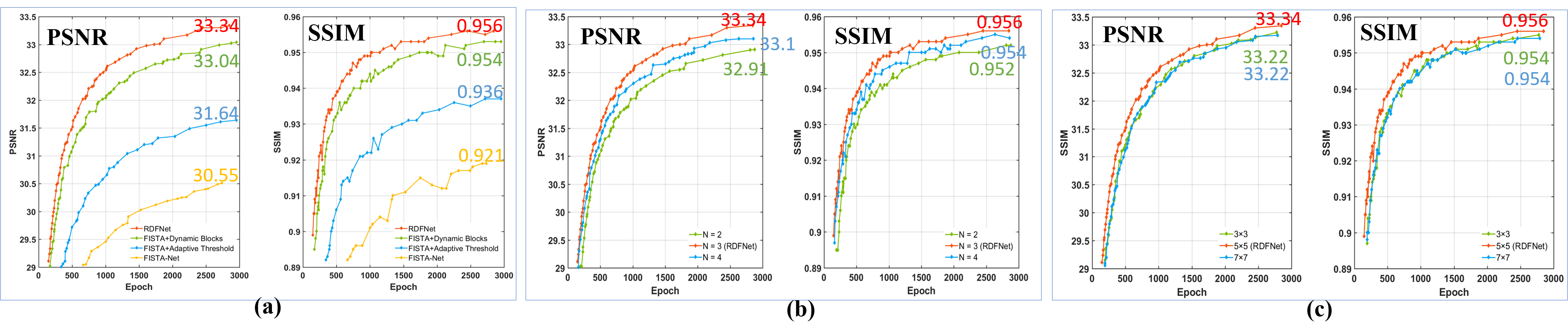
Figure 5: Ablation results. Ablations of (a) regional dynamic block and pixel-wise adaptive soft-thresholding; (b) number of the regional dynamic blocks; (c) regional pooling size.

IV-C Results on Real Data

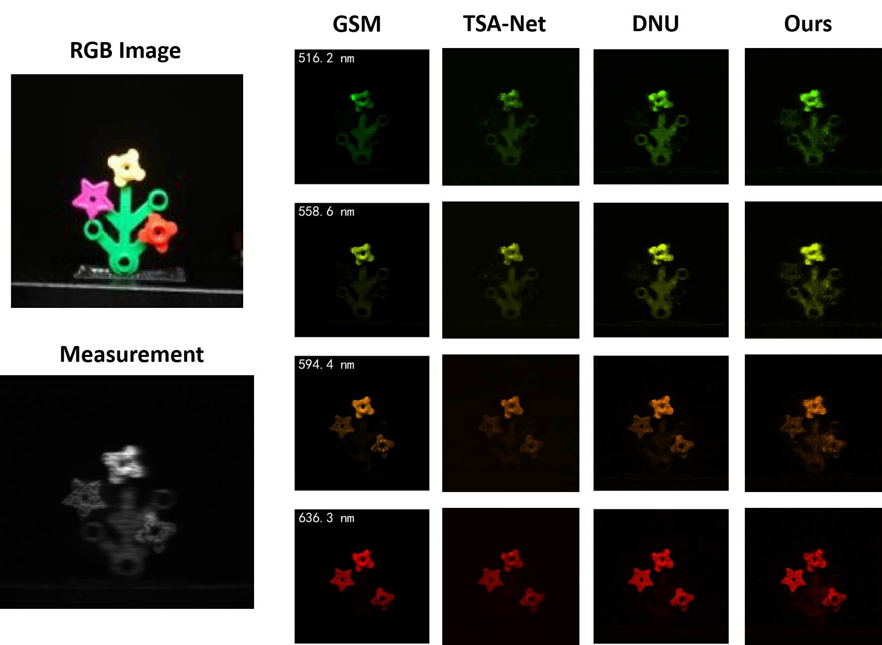
Figure 6: Reconstructed images of the real scene1 with 4 our of 28 spectral channels by the competing methods.

We test our methods on real SD-CASSI data [64, 22] that captures real scenes with $28$ wavelengths ranging from $450\rm{nm}$ to $650\rm{nm}$ and has 54-pixel dispersion in the column dimension. Thus, the measurements captured by the system have a spatial size of $660\times 714$. Fig. 6 shows the reconstruction results of scene1 with four channels by RDFNet and other competing methods. One can observe that our method well recovers textures in both spectral and spatial dimensions.

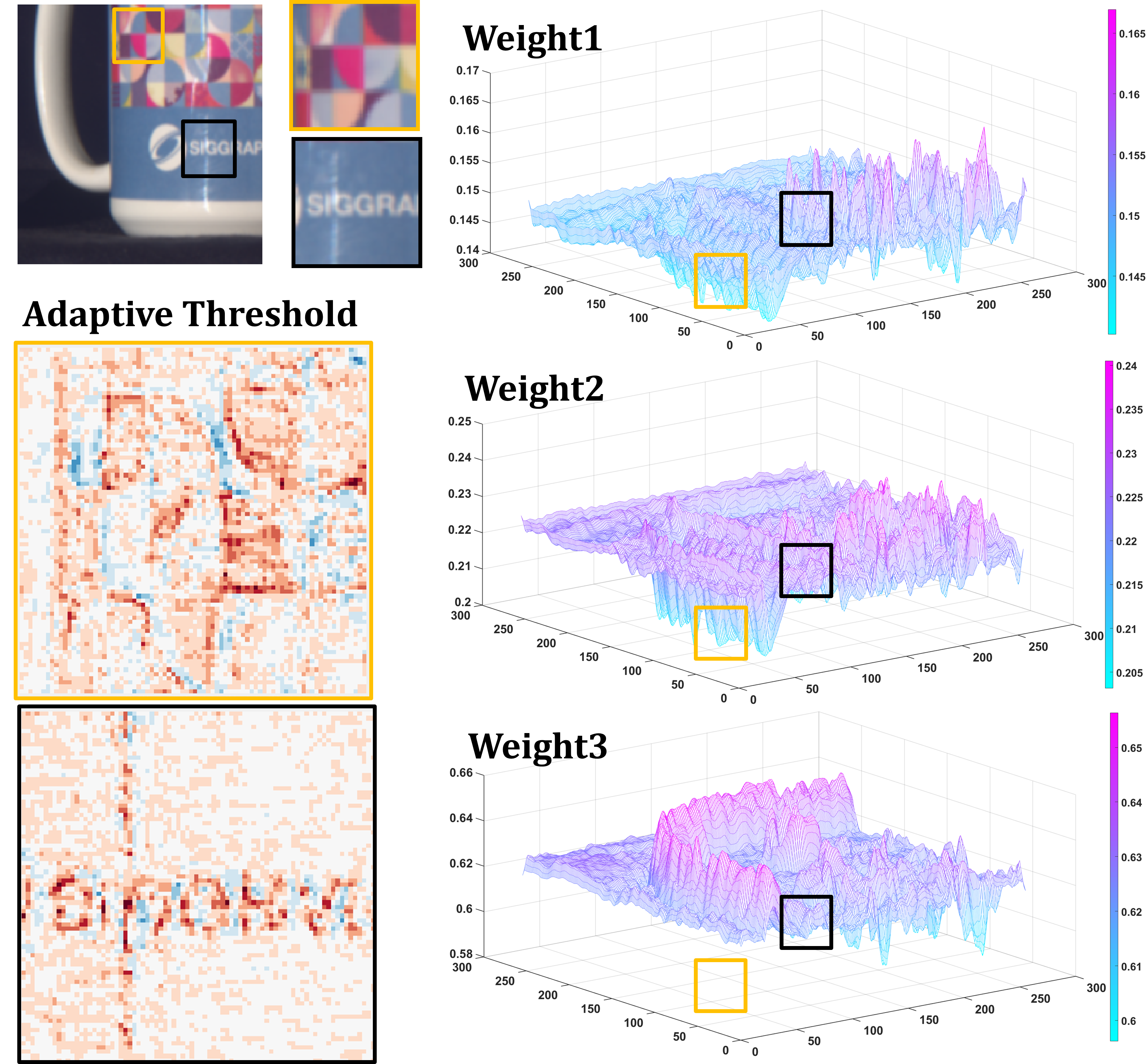
Figure 7: Visualization of dynamic weights in each dynamic block and adaptive soft-thresholding in RDFNet. We randomly selected two regions that were labeled respectively.

IV-D Ablation Studies

Effect of key components. The regional dynamic FISTA network consists of two key components: the region-based dynamic block used to transform different patches into different sparse domains and the pixel-wise adaptive thresholding module used to dynamically determinate appropriate shrinkage scale. We test the effectiveness of each of the two components by incorporating them one-by-one progressively.

As shown in Fig. 5 (a), the quality of reconstruction (evaluated by PSNR and SSIM) is gradually increasing. Our RDFNet achieves the best performance and outperforms the FISTA-Net baseline by $2.79\rm{dB}$ in average PSNR. Tab. V shows the improvements by separately incorporating the dynamic block and adaptive soft-thresholding are $0.3\rm{dB}$ and $1.7\rm{dB}$ in average, respectively. It indicates that the regional dynamic strategy largely contributes to the performance gain and the adaptive soft-thresholding brings additional improvement.

TABLE V: Ablation analysis of key components. AT represents Adaptive Threshold, DB represents Dynamic Blocks.

	AT	DB	PSNR	SSIM
Baseline [25]			30.55	0.921
Baseline+AT	✓		31.64	0.936
Baseline+DB		✓	33.04	0.954
RDFNet(Ours)	✓	✓	33.34	0.956

Impact of block number. To investigate the impact of dynamic block number $N$, we test the model variants with $N=2,3,4$. Fig. 5 (b) shows that our model is not sensitive to the number of dynamic blocks affects reconstruction error but only to a certain extent. The model with $N=3$ achieves the best in both PSNR and SSIM. Decreasing the block number, i.e., $N=2$, leads to slight performance degradation. One possible explanation is that fewer blocks result in fewer transformation domains for dynamic regulation. In addition, increasing the blocks i.e., $N=4$, brings no further performance improvement. The reason is that too many parameters may cause the problem of poor network convergence.

Impact of region pooling. We further study the impact of the kernel size of regional pooling in Fig. 5 (c). We test the model variants with pooling kernel size of $3\times 3$, $5\times 5$, and $7\times 7$. The model with $5\times 5$ pooling performs the best. A smaller $3\times 3$ pooling kernel, which leads to more fine-grained region division, affects the extraction of regional characteristics and thus hinders the dynamic adjustment of transformation domain. While a larger $7\times 7$ kernel blurs the region division and leads to unreasonable weights allocation.

V Conclusion

We have proposed a regional dynamic FISTA algorithm for coded aperture snapshot spectral imaging. Unlike the existing static transformation network, we develop a novel hierarchical regional dynamic structure that adjusts different regions into adaptive transformations according to their characteristics. Besides, a pixel-wise attention strategy have been used on soft-thresholding. Extensive experiments show that the proposed RDFNet achieves the best reconstruction results, demonstrating clear superiority over prior state-of-the-arts in terms of both accuracy and efficiency. Specifically, the proposed RDFNet achieves an average PSNR of $35.51\rm{dB}$ among seven mainstream methods on the ICVL [30] and $33.34\rm{dB}$ among fourteen kinds of HSI reconstruction methods on the KAIST [28]. While on the parameters analysis, our proposd method achieves only 1.29M parameters and inference time of 0.11 second per-image and obtains competitive results on the FLOPs.

Our proposed method is not limited to spectral SCI. It can also be used in video SCI systems. One future direction of interest is to extend the dynamic transform domain to other tasks.

Shiyun Zhou is currently pursuing the M.S. degree with the School of Optics and Photonics, Beijing Institute of Technology, Beijing, China. Her research interests include hyperspectral image processing and compressive spectral reconstruction.

Tingfa Xu received the Ph.D. degree from the Changchun Institute of Optics, Fine Mechanics and Physics, Changchun, China, in 2004. He is currently a Professor with the School of Optics and Photonics, Beijing Institute of Technology, Beijing, China. His research interests include optoelectronic imaging and detection and hyperspectral remote sensing image processing.

Shaocong Dong is currently pursuing the M.S. degree with the School of Optics and Photonics, Beijing Institute of Technology, Beijing, China. His research interests include hyperspectral image processing, 3d point cloud data processing and compressive spectral reconstruction.

Jianan Li is currently an assistant professor at School of Optics and Photonics, Beijing Institute of Technology, Beijing, China, where he received his B.S. and Ph.D. degree in 2013 and 2019, respectively. From July 2015 to July 2017, he worked as a joint training Ph.D. student at National University of Singapore. From October 2017 to April 2018, he worked as an intern at Adobe Research. His research interests mainly include computer vision and real-time image/video processing.

References

- [1] M. Borengasser, W. S. Hungate, and R. Watkins, Hyperspectral remote sensing: principles and applications. CRC press, 2007.
- [2] V. Backman, M. B. Wallace, L. Perelman, J. Arendt, R. Gurjar, M. Müller, Q. Zhang, G. Zonios, E. Kline, T. McGillican et al., “Detection of preinvasive cancer cells,” Nature, vol. 406, no. 6791, pp. 35–36, 2000.
- [3] Q. Li, X. He, Y. Wang, H. Liu, D. Xu, and F. Guo, “Review of spectral imaging technology in biomedical engineering: achievements and challenges,” Journal of biomedical optics, vol. 18, no. 10, p. 100901, 2013.
- [4] M. Kubik, “Hyperspectral imaging: a new technique for the non-invasive study of artworks,” in Physical techniques in the study of art, archaeology and cultural heritage. Elsevier, 2007, vol. 2, pp. 199–259.
- [5] Y.-Z. Feng and D.-W. Sun, “Application of hyperspectral imaging in food safety inspection and control: a review,” Critical reviews in food science and nutrition, vol. 52, no. 11, pp. 1039–1058, 2012.
- [6] M. Moroni, E. Lupo, E. Marra, and A. Cenedese, “Hyperspectral image analysis in environmental monitoring: setup of a new tunable filter platform,” Procedia Environmental Sciences, vol. 19, pp. 885–894, 2013.
- [7] G. Vane, R. O. Green, T. G. Chrien, H. T. Enmark, E. G. Hansen, and W. M. Porter, “The airborne visible/infrared imaging spectrometer (aviris),” Remote sensing of environment, vol. 44, no. 2-3, pp. 127–143, 1993.
- [8] L. J. Rickard, R. W. Basedow, E. F. Zalewski, P. R. Silverglate, and M. Landers, “Hydice: An airborne system for hyperspectral imaging,” in Imaging Spectrometry of the Terrestrial Environment, vol. 1937. SPIE, 1993, pp. 173–179.
- [9] N. Gat, “Imaging spectroscopy using tunable filters: a review,” Wavelet Applications VII, vol. 4056, pp. 50–64, 2000.
- [10] N. A. Hagen and M. W. Kudenov, “Review of snapshot spectral imaging technologies,” Optical Engineering, vol. 52, no. 9, p. 090901, 2013.
- [11] A. Kawai, T. Kageyama, R. Horisaki, and T. Ideguchi, “Compressive dual-comb spectroscopy,” Scientific Reports, vol. 11, no. 1, pp. 1–8, 2021.
- [12] L. Huang, R. Luo, X. Liu, and X. Hao, “Spectral imaging with deep learning,” Light: Science & Applications, vol. 11, no. 1, pp. 1–19, 2022.
- [13] J. Zhang, R. Su, Q. Fu, W. Ren, F. Heide, and Y. Nie, “A survey on computational spectral reconstruction methods from rgb to hyperspectral imaging,” Scientific reports, vol. 12, no. 1, pp. 1–17, 2022.
- [14] D. L. Donoho, “Compressed sensing,” IEEE Transactions on information theory, vol. 52, no. 4, pp. 1289–1306, 2006.
- [15] E. J. Candès, J. Romberg, and T. Tao, “Robust uncertainty principles: Exact signal reconstruction from highly incomplete frequency information,” IEEE Transactions on information theory, vol. 52, no. 2, pp. 489–509, 2006.
- [16] G. R. Arce, D. J. Brady, L. Carin, H. Arguello, and D. S. Kittle, “Compressive coded aperture spectral imaging: An introduction,” IEEE Signal Processing Magazine, vol. 31, no. 1, pp. 105–115, 2013.
- [17] A. Wagadarikar, R. John, R. Willett, and D. Brady, “Single disperser design for coded aperture snapshot spectral imaging,” Applied optics, vol. 47, no. 10, pp. B44–B51, 2008.
- [18] X. Yuan, “Generalized alternating projection based total variation minimization for compressive sensing,” in 2016 IEEE International Conference on Image Processing (ICIP). IEEE, 2016, pp. 2539–2543.
- [19] D. P. Kingma and J. Ba, “Adam: A method for stochastic optimization,” arXiv preprint arXiv:1412.6980, 2014.
- [20] J. M. Bioucas-Dias and M. A. Figueiredo, “A new twist: Two-step iterative shrinkage/thresholding algorithms for image restoration,” IEEE Transactions on Image processing, vol. 16, no. 12, pp. 2992–3004, 2007.
- [21] S. Zheng, Y. Liu, Z. Meng, M. Qiao, Z. Tong, X. Yang, S. Han, and X. Yuan, “Deep plug-and-play priors for spectral snapshot compressive imaging,” Photonics Research, vol. 9, no. 2, pp. B18–B29, 2021.
- [22] Z. Meng, J. Ma, and X. Yuan, “End-to-end low cost compressive spectral imaging with spatial-spectral self-attention,” in European Conference on Computer Vision. Springer, 2020, pp. 187–204.
- [23] L. Wang, C. Sun, M. Zhang, Y. Fu, and H. Huang, “Dnu: deep non-local unrolling for computational spectral imaging,” in Proceedings of the IEEE/CVF Conference on Computer Vision and Pattern Recognition, 2020, pp. 1661–1671.
- [24] X. Miao, X. Yuan, Y. Pu, and V. Athitsos, “l-net: Reconstruct hyperspectral images from a snapshot measurement,” in Proceedings of the IEEE/CVF International Conference on Computer Vision, 2019, pp. 4059–4069.
- [25] X. Han, B. Wu, Z. Shou, X.-Y. Liu, Y. Zhang, and L. Kong, “Tensor fista-net for real-time snapshot compressive imaging,” in Proceedings of the AAAI Conference on Artificial Intelligence, vol. 34, no. 07, 2020, pp. 10 933–10 940.
- [26] J. Ma, X.-Y. Liu, Z. Shou, and X. Yuan, “Deep tensor admm-net for snapshot compressive imaging,” in Proceedings of the IEEE/CVF International Conference on Computer Vision, 2019, pp. 10 223–10 232.
- [27] A. Beck and M. Teboulle, “A fast iterative shrinkage-thresholding algorithm for linear inverse problems,” SIAM journal on imaging sciences, vol. 2, no. 1, pp. 183–202, 2009.
- [28] I. Choi, M. Kim, D. Gutierrez, D. Jeon, and G. Nam, “High-quality hyperspectral reconstruction using a spectral prior,” Tech. Rep., 2017.
- [29] F. Yasuma, T. Mitsunaga, D. Iso, and S. K. Nayar, “Generalized assorted pixel camera: postcapture control of resolution, dynamic range, and spectrum,” IEEE transactions on image processing, vol. 19, no. 9, pp. 2241–2253, 2010.
- [30] B. Arad and O. Ben-Shahar, “Sparse recovery of hyperspectral signal from natural rgb images,” in European Conference on Computer Vision. Springer, 2016, pp. 19–34.
- [31] Y. Chen, X. Dai, M. Liu, D. Chen, L. Yuan, and Z. Liu, “Dynamic convolution: Attention over convolution kernels,” in Proceedings of the IEEE/CVF Conference on Computer Vision and Pattern Recognition, 2020, pp. 11 030–11 039.
- [32] X. Jia, B. De Brabandere, T. Tuytelaars, and L. V. Gool, “Dynamic filter networks,” Advances in neural information processing systems, vol. 29, pp. 667–675, 2016.
- [33] B. Yang, G. Bender, Q. V. Le, and J. Ngiam, “Condconv: Conditionally parameterized convolutions for efficient inference,” arXiv preprint arXiv:1904.04971, 2019.
- [34] M. Xu, R. Ding, H. Zhao, and X. Qi, “Paconv: Position adaptive convolution with dynamic kernel assembling on point clouds,” in Proceedings of the IEEE/CVF Conference on Computer Vision and Pattern Recognition, 2021, pp. 3173–3182.
- [35] L. Zhang, Z. Lang, P. Wang, W. Wei, S. Liao, L. Shao, and Y. Zhang, “Pixel-aware deep function-mixture network for spectral super-resolution,” in Proceedings of the AAAI Conference on Artificial Intelligence, vol. 34, no. 07, 2020, pp. 12 821–12 828.
- [36] J. Bacca, Y. Fonseca, and H. Arguello, “Compressive spectral image reconstruction using deep prior and low-rank tensor representation,” Appl. Opt., vol. 60, no. 14, pp. 4197–4207, May 2021. [Online]. Available: http://opg.optica.org/ao/abstract.cfm?URI=ao-60-14-4197
- [37] D. Van Veen, A. Jalal, M. Soltanolkotabi, E. Price, S. Vishwanath, and A. G. Dimakis, “Compressed sensing with deep image prior and learned regularization,” arXiv preprint arXiv:1806.06438, 2018.
- [38] T. Gelvez, J. Bacca, and H. Arguello, “Interpretable deep image prior method inspired in linear mixture model for compressed spectral image recovery,” in 2021 IEEE International Conference on Image Processing (ICIP). IEEE, 2021, pp. 1934–1938.
- [39] L. Wang, C. Sun, Y. Fu, M. H. Kim, and H. Huang, “Hyperspectral image reconstruction using a deep spatial-spectral prior,” in Proceedings of the IEEE/CVF Conference on Computer Vision and Pattern Recognition, 2019, pp. 8032–8041.
- [40] G. Mataev, P. Milanfar, and M. Elad, “Deepred: Deep image prior powered by red,” in Proceedings of the IEEE/CVF International Conference on Computer Vision Workshops, 2019, pp. 0–0.
- [41] Y. Romano, M. Elad, and P. Milanfar, “The little engine that could: Regularization by denoising (red),” SIAM Journal on Imaging Sciences, vol. 10, no. 4, pp. 1804–1844, 2017.
- [42] Z. Meng, Z. Yu, K. Xu, and X. Yuan, “Self-supervised neural networks for spectral snapshot compressive imaging,” in Proceedings of the IEEE/CVF International Conference on Computer Vision, 2021, pp. 2622–2631.
- [43] O. Ronneberger, P. Fischer, and T. Brox, “U-net: Convolutional networks for biomedical image segmentation,” in International Conference on Medical image computing and computer-assisted intervention. Springer, 2015, pp. 234–241.
- [44] I. Goodfellow, J. Pouget-Abadie, M. Mirza, B. Xu, D. Warde-Farley, S. Ozair, A. Courville, and Y. Bengio, “Generative adversarial nets,” Advances in neural information processing systems, vol. 27, 2014.
- [45] S. H. Chan, X. Wang, and O. A. Elgendy, “Plug-and-play admm for image restoration: Fixed-point convergence and applications,” IEEE Transactions on Computational Imaging, vol. 3, no. 1, pp. 84–98, 2016.
- [46] X. Yuan, Y. Liu, J. Suo, F. Durand, and Q. Dai, “Plug-and-play algorithms for video snapshot compressive imaging,” arXiv preprint arXiv:2101.04822, 2021.
- [47] Z. Meng, S. Jalali, and X. Yuan, “Gap-net for snapshot compressive imaging,” arXiv preprint arXiv:2012.08364, 2020.
- [48] T. Huang, W. Dong, X. Yuan, J. Wu, and G. Shi, “Deep gaussian scale mixture prior for spectral compressive imaging,” in Proceedings of the IEEE/CVF Conference on Computer Vision and Pattern Recognition, 2021, pp. 16 216–16 225.
- [49] S. Zhang, L. Wang, L. Zhang, and H. Huang, “Learning tensor low-rank prior for hyperspectral image reconstruction,” in Proceedings of the IEEE/CVF Conference on Computer Vision and Pattern Recognition, 2021, pp. 12 006–12 015.
- [50] K. Zhang, W. Zuo, and L. Zhang, “Ffdnet: Toward a fast and flexible solution for cnn-based image denoising,” IEEE Transactions on Image Processing, vol. 27, no. 9, pp. 4608–4622, 2018.
- [51] X. Yuan, Y. Liu, J. Suo, and Q. Dai, “Plug-and-play algorithms for large-scale snapshot compressive imaging,” in Proceedings of the IEEE/CVF Conference on Computer Vision and Pattern Recognition, 2020, pp. 1447–1457.
- [52] X. Yuan, D. J. Brady, and A. K. Katsaggelos, “Snapshot compressive imaging: Theory, algorithms, and applications,” IEEE Signal Processing Magazine, vol. 38, no. 2, pp. 65–88, 2021.
- [53] M. Elad and M. Aharon, “Image denoising via sparse and redundant representations over learned dictionaries,” IEEE Transactions on Image processing, vol. 15, no. 12, pp. 3736–3745, 2006.
- [54] Y. Wang, J. Yang, W. Yin, and Y. Zhang, “A new alternating minimization algorithm for total variation image reconstruction,” SIAM Journal on Imaging Sciences, vol. 1, no. 3, pp. 248–272, 2008.
- [55] M. F. Tappen, “Utilizing variational optimization to learn markov random fields,” in 2007 IEEE Conference on Computer Vision and Pattern Recognition. IEEE, 2007, pp. 1–8.
- [56] R. Tibshirani, “Regression shrinkage and selection via the lasso,” Journal of the Royal Statistical Society: Series B (Methodological), vol. 58, no. 1, pp. 267–288, 1996.
- [57] D. L. Donoho, “De-noising by soft-thresholding,” IEEE transactions on information theory, vol. 41, no. 3, pp. 613–627, 1995.
- [58] K. He, X. Zhang, S. Ren, and J. Sun, “Deep residual learning for image recognition,” in Proceedings of the IEEE conference on computer vision and pattern recognition, 2016, pp. 770–778.
- [59] X. Yuan, “Generalized alternating projection based total variation minimization for compressive sensing,” in 2016 IEEE International Conference on Image Processing (ICIP). IEEE, 2016, pp. 2539–2543.
- [60] Y. Liu, X. Yuan, J. Suo, D. J. Brady, and Q. Dai, “Rank minimization for snapshot compressive imaging,” IEEE transactions on pattern analysis and machine intelligence, vol. 41, no. 12, pp. 2990–3006, 2018.
- [61] Z. Wang, A. C. Bovik, H. R. Sheikh, and E. P. Simoncelli, “Image quality assessment: from error visibility to structural similarity,” IEEE transactions on image processing, vol. 13, no. 4, pp. 600–612, 2004.
- [62] Z. Xiong, Z. Shi, H. Li, L. Wang, D. Liu, and F. Wu, “Hscnn: Cnn-based hyperspectral image recovery from spectrally undersampled projections,” in Proceedings of the IEEE International Conference on Computer Vision Workshops, 2017, pp. 518–525.
- [63] J. Zhang and B. Ghanem, “Ista-net: Interpretable optimization-inspired deep network for image compressive sensing,” in Proceedings of the IEEE conference on computer vision and pattern recognition, 2018, pp. 1828–1837.
- [64] B. Mildenhall, J. T. Barron, J. Chen, D. Sharlet, R. Ng, and R. Carroll, “Burst denoising with kernel prediction networks,” in Proceedings of the IEEE Conference on Computer Vision and Pattern Recognition, 2018, pp. 2502–2510.