Circular and Spherical Projected Cauchy Distributions: A Novel Framework for Circular and Directional Data Modeling

Abstract

We introduce a novel family of projected distributions on the circle and the sphere, namely the circular and spherical projected Cauchy distributions as promising alternatives for modeling circular and directional data. The circular distribution encompasses the wrapped Cauchy distribution as a special case, featuring a more convenient parameterisation. Next, we propose a generalised wrapped Cauchy distribution that includes an extra parameter, enhancing the fit of the distribution. In the spherical context, we impose two conditions on the scatter matrix, resulting in an elliptically symmetric distribution. Our projected distributions exhibit attractive properties, such as closed-form normalising constants and straightforward random value generation. The distribution parameters can be estimated using maximum likelihood and we assess their bias through numerical studies. We compare our proposed distributions to existing models with real data sets, demonstrating superior fit both with and without covariates.

Keywords: Directional data, Cauchy distribution, projected distribution

1 Introduction

Directional data refers to multivariate data with a unit norm, and its sample space can be expressed as:

$$\mathbb{S}^{d-1}=\left\{{\bf x}\in\mathbb{R}^{d}\bigg{|}\left|\left|{\bf x}\right|\right|=1\right\},$$

where $\left|\left|.\right|\right|$ denotes the Euclidean norm. Circular data, when $d=2$, lie on a circle, whereas spherical data, when $d=3$, lie on a sphere. Circular data are met in various disciplines, such as political sciences (Gill and Hangartner, 2010), criminology (Shirota and Gelfand, 2017), biology (Landler et al., 2018), ecology (Horne et al., 2007) and astronomy (Soler et al., 2019) to name a few. Spherical data on the other hand are met in geology (Chang, 1986), environmental sciences (Heaton et al., 2014), image analysis (Straub et al., 2015), robotics (Bullock, Feix and Dollar, 2014) and space (Kent, John T and Hussein, Islam and Jah, Moriba K, 2016).

A vast array of circular distributions exists in the literature, with the earliest being the von Mises distribution (von Mises, 1918), investigated by Mardia (1972), Mardia and Jupp (2000). This distribution emerges as the conditional distribution of a bivariate normal random vector with a specific mean vector and identity covariance matrix, given that the vector resides on the unit sphere. Over the years, various generalisations of this distribution have been proposed (Gatto and Jammalamadaka, 2007, Kim and SenGupta, 2013, Dietrich and Richter, 2017), with additional circular distributions introduced by Pewsey (2000), Jones and Pewsey (2005), Abe and Pewsey (2011), and Jones and Pewsey (2012). Wrapped distributions represent another class of distributions arising from wrapping a univariate random vector on the circle. This category includes the wrapped $t$ family of distributions (Pewsey et al., 2007), the wrapped stable family (Pewsey, 2008), the wrapped normal, and wrapped Cauchy (WC) distributions (Mardia and Jupp, 2000), as well as their extensions (Kato and Jones, 2010, 2013). Lastly, a less explored type of distribution, known as projected distributions, originate from the distribution of a multivariate random vector projected onto a circle. The projected normal (PN) distribution (Watson, 1983, Presnell et al., 1998, Mardia and Jupp, 2000) is likely the only distribution of this kind.

Incorporating more than two parameters in circular probability distributions is a common practice aimed at enhancing flexibility and better capturing skewed data. However, many such distributions assume a diagonal scatter matrix, thereby limiting their capacity to model intricate data structures. The PN distribution, an exception to this issue, encompasses multiple parameters and has been employed to model various data types, including skewed data. The PN distribution differentiates itself from other multidimensional distributions by adopting a Bayesian approach (Nuñez-Antonio and Gutiérrez-Peña, 2005, Wang and Gelfand, 2013, Hernandez-Stumpfhauser and Breidt and van der Woerd, 2017) to estimate distribution parameters, addressing the diagonal scatter matrix problem. This method enables more flexible modeling of complex data structures, such as those with non-diagonal covariance matrices.

Numerous spherical and hyper-spherical distributions have been proposed over time, with the von Mises-Fisher (Fisher, 1953) and PN (Mardia, 1972, Kendall, 1974) distributions being among the earliest and most prevalent, while the spherical Cauchy (SP) (Kato and McCullagh, 2020) is a more recent proposition. However, these distributions assume rotational symmetry, which may restrict their applicability in certain scenarios. To mitigate this constraint, Kent (1982) introduced an elliptically symmetric distribution that relaxes the rotational symmetry assumption. This distribution constitutes a special case of the Fisher-Bingham distribution (Mardia, 1972, 1975) and has proven valuable for modelingore sophisticated data structures. More recently, Paine et al. (2018) proposed the elliptically symmetric angular Gaussian distribution, which emerges by projecting the Gaussian distribution onto the (hyper-)sphere and imposing two conditions on the covariance matrix.

In this study, we introduce the circular and spherical projected Cauchy distributions, representing noteworthy additions to the family of directional distributions, as they provide an alternative perspective on the Cauchy distribution. Notable characteristics of these new distributions include their closed-form normalising constant and the simplicity of simulation, rendering them particularly attractive for modeling directional data. By projecting the bivariate Cauchy distribution onto the circle, we derive a univariate distribution. When the scatter matrix is equivalent to the identity matrix, the resulting distribution corresponds to the wrapped Cauchy (WC) distribution, albeit with a more convenient parameterisation. This significant outcome enables us to associate the circular projected Cauchy with a well-established distribution. Subsequently, in line with Paine et al. (2018), we impose a mean-constrained scatter matrix, offering enhanced flexibility and facilitating more realistic modeling of circular data. The spherical projected Cauchy distribution is also of interest, as it yields an elliptically symmetric distribution for spherical data, a property scarcely encountered in the literature. Imposing the same conditions as in Paine et al. (2018) results in an elliptically symmetric distribution. This characteristic is of paramount importance concerning spherical data, given the limited number of distributions with this property documented in the literature.

We present the proposed circular and spherical projected Cauchy distributions, including the regression setting, in Sections 2 and 3, respectively. To compare the performance of the various forms of the proposed projected Cauchy distributions with one another and with alternative distributions, we conduct simulation studies focusing on the bias of the estimated parameters in Section 4. The performance of the proposed distributions and selective competing distributions is demonstrated using real data examples in Section 5. Section 6 offers concluding remarks on the paper.

2 Circular Projected Cauchy Distribution and Its Special Cases

The probability density function of a d-dimensional random vertor $\bf X$ projected onto a circle/sphere/hypersphere is given by ${\bf Y}=\frac{{\bf X}}{r}$, where $r=\left|\left|{\bf X}\right|\right|$. The marginal distribution of ${\bf Y}$, which is of interest, is obtained by integrating out $r$ over the positive line

$$f({\bf y})=\int_{0}^{\infty}r^{d-1}f(r{\bf y})dr.$$ (1)

The probability density function of the bivariate Cauchy distribution is given by

$$f({\bf x})=\frac{1}{2\pi|\boldsymbol{\Sigma}|^{1/2}}\left[1+\left({\bf x}-\boldsymbol{\mu}\right)^{\top}\boldsymbol{\Sigma}^{-1}\left({\bf x}-\boldsymbol{\mu}\right)\right]^{-3/2}.$$ (2)

By substituting (2) into (1) and evaluating the integral, we arrive at a new distribution on the circle, termed the Circular Projected Cauchy (CPC) distribution.

$$f({\bf y}) = \int_{0}^{\infty}\frac{r}{2\pi|\boldsymbol{\Sigma}|^{1/2}}\left(1+r^{2}{\bf y}^{\top}\boldsymbol{\Sigma}^{-1}{\bf y}-2r{\bf y}^{\top}\boldsymbol{\Sigma}^{-1}\boldsymbol{\mu}+\boldsymbol{\mu}^{\top}\boldsymbol{\Sigma}^{-1}\boldsymbol{\mu}\right)^{-3/2}dr$$ (3)

$$= \frac{1}{2\pi|\boldsymbol{\Sigma}|^{1/2}\left(B\sqrt{\Gamma^{2}+1}-A\sqrt{B}\right)},$$

where $A={\bf y}^{\top}\boldsymbol{\Sigma}^{-1}\boldsymbol{\mu}$, $B={\bf y}^{\top}\boldsymbol{\Sigma}^{-1}{\bf y}$, and $\Gamma^{2}=\boldsymbol{\mu}^{\top}\boldsymbol{\Sigma}^{-1}\boldsymbol{\mu}$. It is important to note that ${\bf y}\in\mathbb{S}^{1}$, while $\bm{\mu}\in\mathbb{R}^{2}$.

2.1 The WC as a Special Case of the CPC Distribution

The difficulty with the CPC is the excessive number of parameters, leading to over-identifiability issues during the estimation process. To avoid this, we assume $\boldsymbol{\Sigma}={\bf I}_{2}$, resulting in the following representation:

$$f({\bf y})=\dfrac{1}{2\pi\left(\sqrt{\gamma^{2}+1}-\alpha\right)},$$ (4)

where $\alpha={\bf y}^{\top}\boldsymbol{\mu}$ and $\gamma=|\boldsymbol{\mu}|$. The density in (4) can also be written as

$$f({\bf\theta})=\dfrac{1}{2{\pi}\left(\sqrt{\gamma^{2}+1}-\gamma\cos{\left(\theta-\omega\right)}\right)}$$ (5)

since $\alpha=\gamma\cos{\left(\theta-\omega\right)}$, where $\omega$ denotes the mean. When $\gamma=0$, the distribution reduces to the circular uniform, with a density function given by $f\left(\theta\right)=\left(2\pi\right)^{-1}$. We will denote the distribution with the density given in (4) as the Circular Independent Projected Cauchy (CIPC) distribution.

Consider now a random variable $X$ on the real line, which we wrap around the circumference of a circle with unit radius by $\theta=X(\mod{2\pi})$. If $X$ follows the Cauchy distribution, then $\theta$ follows the WC distribution on the circle, and its density function is given by (Mardia and Jupp, 2000):

$$f(\theta)=\frac{1-\lambda^{2}}{2\pi\left[1+\lambda^{2}-2\lambda\cos\left(\theta-\omega\right)\right]},$$ (6)

where $\omega$ denotes the mean, and $\lambda\in[0,1)$. A close examination reveals that the density in (4) is a different parameterisation of the WC distribution in (6), where $\sqrt{\gamma^{2}+1}=\frac{1+\rho^{2}}{1-\rho^{2}}$ and $\gamma=\frac{2\rho}{1-\rho^{2}}$, or conversely, $\rho=(\sqrt{\gamma^{2}+1}-1)/\gamma$. This remarkable result shows that the Wrapped Cauchy distribution can also be obtained by projecting the bivariate Cauchy distribution onto the circle. This appealing equivalence is not observed for the Wrapped Normal and the PN (Presnell et al., 1998). The question of whether there are more wrapped distributions that can be created by projection is now raised.

Jones and Pewsey (2005) mentioned that the wrapped Cauchy is the only member of their suggested family of symmetric unimodal distributions that arise by projection onto, rather than conditioning on, the unit circle. Specifically, as pointed out in (Mardia and Jupp, 2000), if $\theta$ follows the angular central Gaussian distribution, then $2\theta$ follows the WC. They also stated that … the WC distribution does not arise from projecting a bivariate spherically symmetric distribution with non-zero mean onto the circle.. According to our previous results, this statement is not entirely accurate. Furthermore, the fact that we derived the WC via a different route enables us to generalise the WC distribution in a straightforward manner, as described in the subsequent section.

2.2 The Generalised Circular Projected Cauchy Distribution

A common issue with circular distributions is that, in the two-dimensional space, they impose no correlation between the components. We relax this strict assumption by employing one of the conditions imposed in Paine et al. (2018), that is, $\boldsymbol{\Sigma\mu}=\boldsymbol{\mu}$, but not $|\boldsymbol{\Sigma}|=1$. This condition implies that the leading eigenvector $\boldsymbol{\xi}_{1}$ of $\boldsymbol{\Sigma}$ is the normalised mean vector $\boldsymbol{\xi}_{1}=\left(\mu_{1},\mu_{2}\right)^{\top}/\gamma$, while the second eigenvector can be defined up to the sign as $\boldsymbol{\xi}_{2}=\left(-\mu_{2},\mu_{1}\right)^{\top}/\gamma$ or $\boldsymbol{\xi}_{2}=\left(\mu_{2},-\mu_{1}\right)^{\top}/\gamma$. The leading eigenvalue is equal to 1, while the second eigenvalue is equal to $\rho\in(0,1]$, hence $|\boldsymbol{\Sigma}|=\rho$ and the inverse of the scatter matrix is given by

$$\boldsymbol{\Sigma}^{-1}=\frac{1}{\gamma^{2}}\left(\begin{array}[]{cc}\mu_{1}^{2}+\mu_{2}^{2}/\rho&\mu_{1}\mu_{2}\left(1-1/\rho\right)\\ \mu_{1}\mu_{2}\left(1-1/\rho\right)&\mu_{2}^{2}+\mu_{1}^{2}/\rho\end{array}\right)=\boldsymbol{\xi}_{1}\boldsymbol{\xi}_{1}^{\top}+\boldsymbol{\xi}_{2}\boldsymbol{\xi}_{2}^{\top}/\rho.$$ (9)

Thus, (3) becomes

$$f({\bf y})=\frac{1}{2\pi\rho^{1/2}\left(B\sqrt{\gamma^{2}+1}-\alpha\sqrt{B}\right)}.$$ (10)

Utilising (9) and after some calculations, the density in (10) may also be expressed in polar coordinates by

$$f(\theta) = \frac{1}{2\pi\rho^{1/2}\left[\left(\cos^{2}(\theta-\omega)+\frac{\sin^{2}(\theta-\omega)}{\rho}\right)\sqrt{\gamma^{2}+1}-\gamma\cos(\theta-\omega)\sqrt{\cos^{2}(\theta-\omega)+\frac{\sin^{2}(\theta-\omega)}{\rho}}\right]}$$

$$f(\theta) = \frac{1}{2\pi\rho^{1/2}\left(b\sqrt{\gamma^{2}+1}-a\sqrt{b}\right)},$$ (11)

where $b=\cos^{2}(\theta-\omega)+\frac{\sin^{2}(\theta-\omega)}{\rho}$. Alternatively, (2.2) may be written as

$$f(\theta)=\frac{1}{2\pi\rho^{1/2}\cos^{2}(\theta-\omega)\sqrt{1+\frac{\tan^{2}(\theta-\omega)}{\rho}}\left(\sqrt{\left(\gamma^{2}+1\right)\left(1+\frac{\tan^{2}(\theta-\omega)}{\rho}\right)}-\gamma\right)}.$$ (12)

We will call the distribution whose density is given by (10)-(12) the generalised circular projected Cauchy (GCPC) distribution. It is important to note that if $\rho=1$, the GCPC distribution reduces to the CIPC distribution (4). The GCPC distribution exhibits symmetry with respect to $\theta$, such that $f(\theta-\omega)=f(\omega-\theta)$ and is thus symmetrical about $\mu+\pi$. Regrettably, there is no closed form for the cumulative distribution function, trigonometric characteristic function, the mean resultant, and its length. This necessitates the application of numerical integration techniques to compute these quantities. The distribution displays bimodality, which can be easily observed by examining the first derivative of the density (2.2)

$$\frac{\partial\log(f(\theta))}{\partial\omega}=\frac{\left(\left(2{\rho}-2\right)\sqrt{{\gamma}^{2}+1}\cos\left({\theta}-{\omega}\right)\sqrt{\frac{\left({\rho}-1\right)\cos^{2}\left({\theta}-{\omega}\right)+1}{{\rho}}}+\left(2-2{\rho}\right){\gamma}\cos^{2}\left({\theta}-{\omega}\right)-{\gamma}\right)\sin\left({\theta}-{\omega}\right)}{\left(\left({\rho}-1\right)\cos^{2}\left({\theta}-{\omega}\right)+1\right)\left(\sqrt{{\gamma}^{2}+1}\sqrt{\frac{\left({\rho}-1\right)\cos^{2}\left({\theta}-{\omega}\right)+1}{{\rho}}}-{\gamma}\cos\left({\theta}-{\omega}\right)\right)}$$

Setting the above expression to zero, we obtain

$$\left(\left(2{\rho}-2\right)\sqrt{{\gamma}^{2}+1}\cos\left({\theta}-{\omega}\right)\sqrt{\frac{\left({\rho}-1\right)\cos^{2}\left({\theta}-{\omega}\right)+1}{{\rho}}}+\left(2-2{\rho}\right){\gamma}\cos^{2}\left({\theta}-{\omega}\right)-{\gamma}\right)\sin\left({\theta}-{\omega}\right)=0.$$

By conducting the same computations as in Kato and Jones (2010), we observe that the aforementioned equation results in a quartic equation with either four real roots or four complex roots if its discriminant is positive, or two real roots and two complex roots if its discriminant is negative. This finding confirms that the density has at most two modes. Furthermore, the distribution is bimodal when the discriminant is positive and unimodal when the discriminant is negative.

Maximum likelihood estimation of the parameters can be achieved through the Newton-Raphson algorithm; however, the corresponding derivatives are highly complex and extensive. Consequently, we resort to numerical optimisers, such as the simplex algorithm proposed by Nelder and Mead (1965), which is accessible in R through the optim() function. Generating random values from the GCPC distribution is straightforward, requiring only the creation of random vectors from the bivariate Cauchy distribution with a mean-constrained scatter matrix and subsequent normalisation by dividing by their norm.

Figure 1 illustrates the GCPC distribution for various values of $\rho$ and $\gamma$. It is worth noting that alternative restrictions or parameterisations, including the addition of an extra parameter (e.g., isotropic scatter matrix or a non-zero correlation), could also be utilised.

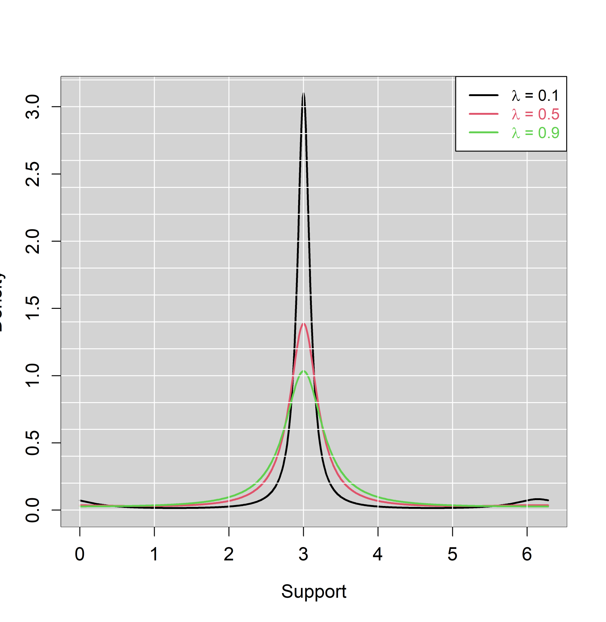
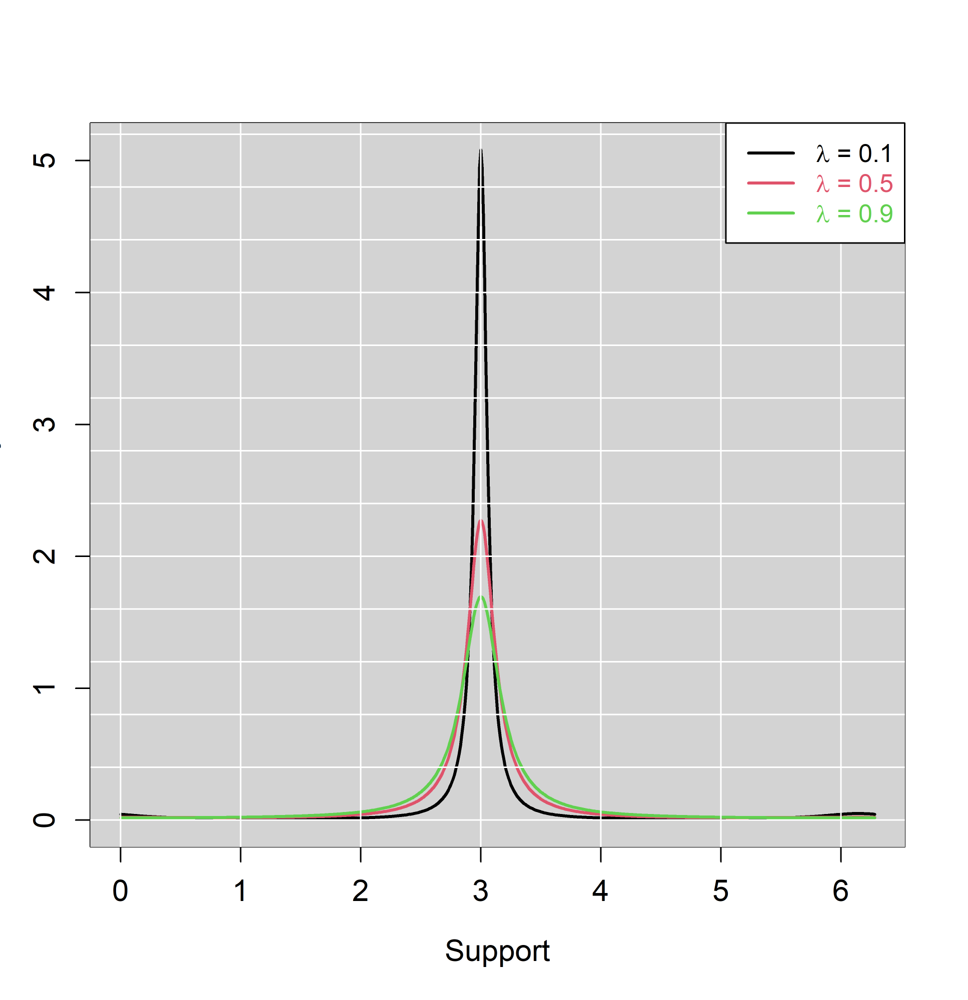
(a) GCPC distribution with $\gamma=3$	(b) GCPC distribution with $\gamma=5$

Figure 1: Densities of the GCPC distribution with (a) $\gamma=3$ and (b) $\gamma=5$, and $\rho=(0.1,0.5,0.9)$.

2.3 Circular Regression

The regression setting is straightforward to implement. The response angular data are transformed into their Euclidean coordinates, and the mean vector is linked to the covariates in the same way as the spherically projected multivariate linear (SPML) model of Presnell et al. (1998).

2.3.1 The SPML Regression Model

The density of the PN is given by

$$f(\theta)=\frac{1}{2\pi e^{-\gamma^{2}/2}}\left[1+\frac{\gamma\cos(\theta-\omega)\Phi\left(\gamma\cos(\theta-\omega)\right)}{\phi(\gamma\cos(\theta-\omega))}\right],$$ (13)

where $\phi(.)$ and $\Phi(.)$ are the standard normal density and distribution functions, respectively. Eq. (13) can also be written as

$$f\left({\bf y}\right)=\frac{1}{2\pi e^{-\gamma^{2}/2}}\left[1+\frac{{\bf y}^{\top}\bm{\mu}\Phi\left({\bf y}^{\top}\bm{\mu}\right)}{\phi({\bf y}^{\top}\bm{\mu})}\right],$$ (14)

where $\bm{\mu}\in\mathbb{R}^{2}$ denotes the mean vector of the bivariate normal. Presnell et al. (1998) linked the mean vector to some covariates $\bf X$, i.e. $\bm{\mu}_{i}=\left(\mu_{1i},\mu_{2i}\right)^{\top}=\left(\bm{\beta}_{1}^{\top}x_{i},\bm{\beta}_{2}^{\top}x_{i}\right)^{\top}={\bf B}^{\top}{\bf x}_{i}$, where ${\bf B}=\left(\bm{\beta}_{1}^{\top},\bm{\beta}_{2}^{\top}\right)^{\top}$ denotes the matrix of the regression coefficients. The relevant log-likelihood, using (14), becomes

$$\ell_{PN}=-\frac{1}{2}\sum_{i=1}^{n}\bm{\mu}_{i}^{\top}\bm{\mu}_{i}+\sum_{i=1}^{n}\log{\left[1+\frac{\bm{\mu}_{i}\Phi\left(\bm{\mu}_{i}\right)}{\phi\left(\bm{\mu}_{i}\right)}\right]}-n\log\left(2\pi\right).$$ (15)

Maximisation of (15) with respect to the matrix of the regression coefficients ${\bf B}$ takes place using the Newton-Raphson algorithm (Presnell et al., 1998). Note also that $\gamma_{i}=\|\bm{\mu}_{i}\|=\left[\left(\bm{\beta}_{1}^{\top}x_{i}\right)^{2}+\left(\bm{\beta}_{2}^{\top}x_{i}\right)^{2}\right]^{1/2}$.

2.3.2 The CIPC and GCPC Regression Models

The log-likelihood of the CIPC regression model is written as

$$\ell_{CIPC}=-\sum_{i=1}^{n}\log{\left(\sqrt{\bm{\mu}_{i}^{\top}\bm{\mu}_{i}+1}-{\bf y}_{i}^{\top}\bm{\mu}_{i}\right)}-n\log{(2\pi)}.$$ (16)

It is important to observe that (16) diverges from the corresponding log-likelihood of the WC distribution (6) in two primary aspects. Firstly, the bivariate representation (Euclidean coordinates) of the angular data is considered, as opposed to their univariate nature. Secondly, the concentration parameter ($\lambda$) of the WC distribution is not maintained as a constant; rather, under the new parametrisation defined in (4), it is contingent upon $\bm{\mu}_{i}$. This is akin to the approach employed in the SPML model, as detailed by Presnell et al. (1998). The log-likelihood of the GCPC regression model is written as

$$\ell_{GCPC}=-\sum_{i=1}^{n}\log{\left({\bf y}_{i}^{\top}\bm{\Sigma}^{-1}_{i}\left({\bf B}\right){\bf y}_{i}\sqrt{\bm{\mu}_{i}^{\top}\bm{\mu}_{i}+1}-{\bf y}_{i}^{\top}\bm{\mu}_{i}\sqrt{{\bf y}_{i}^{\top}\bm{\Sigma}^{-1}_{i}\left({\bf B}\right){\bf y}_{i}}\right)}-n\log(\rho)-n\log{(2\pi)},$$ (17)

where

$$\bm{\Sigma}^{-1}_{i}\left({\bf B}\right) = \bm{\xi}_{1i}\left({\bf B}\right)\bm{\xi}_{1i}\left({\bf B}\right)^{\top}+\bm{\xi}_{2i}\left({\bf B}\right)\bm{\xi}_{2i}\left({\bf B}\right)^{\top}/\rho$$

$$= y_{1i}^{2}\left(\xi_{1i}^{2}+\xi_{2i}^{2}/\rho\right)+y_{2i}^{2}\left(\xi_{2i}^{2}+\xi_{1i}^{2}/\rho\right)+2y_{1i}y_{2i}\xi_{1i}\xi_{2i}\left(1-1/\rho\right)$$

and $\xi_{ji}=\frac{\bm{\beta}_{j}^{\top}x_{i}}{\|\bm{\beta}_{j}^{\top}x_{i}\|}=\frac{\mu_{ji}}{\|\bm{\mu}_{i}\|}=\frac{\mu_{ji}}{\gamma_{i}}$ for $j=1,2$.

The maximisation of (16) is accomplished through the application of Nelder and Mead’s simplex method within the R programming environment. In the case of (17), the same optimisation technique is employed, albeit with a significant distinction. The importance of the initial values necessitates the utilisation of multiple random starts. The presence of $\rho$ adds complexity to the task; to address this issue, the profile log-likelihood of $\rho$ is initially maximised using multiple starting values (e.g., 50 iterations) for the regression coefficients. Subsequently, the resulting optimal values of $\rho$ and the regression coefficients are incorporated as the initial values in a final optimisation procedure.

3 Spherical Projected Cauchy Distribution

The density of the Cauchy distribution in $\mathbb{R}^{3}$ with some scatter matrix and a mean vector $\bm{\mu}\in\mathbb{R}^{3}$ is given by

$$f({\bf x})=\frac{\Gamma(2)}{\Gamma(0.5)\pi^{3/2}|\boldsymbol{\Sigma}|^{1/2}}\left[1+\left({\bf x}-\boldsymbol{\mu}\right)^{\top}\boldsymbol{\Sigma}^{-1}\left({\bf x}-\boldsymbol{\mu}\right)\right]^{-2}=\frac{1}{\pi^{2}|\boldsymbol{\Sigma}|^{1/2}}\left[1+\left({\bf x}-\boldsymbol{\mu}\right)^{\top}\boldsymbol{\Sigma}^{-1}\left({\bf x}-\boldsymbol{\mu}\right)\right]^{-2}.$$

Following the same procedure as before, it turns out that the probability density function of the projected Cauchy variable ${\bf Y}\in\mathbf{S}^{2}$ is given by

$$f({\bf y}) = \int_{0}^{\infty}\frac{r^{2}}{\pi^{2}|\boldsymbol{\Sigma}|^{1/2}\left[1+\left(r{\bf y}-\boldsymbol{\mu}\right)^{\top}\boldsymbol{\Sigma}^{-1}\left({r\bf y}-\boldsymbol{\mu}\right)\right]^{2}}dr$$ (18)

$$= \dfrac{B\left(\gamma^{2}+1\right)\sqrt{\Delta}\left[\operatorname{arctan2}\left(\sqrt{\Delta},-A\right)-\operatorname{arctan2}\left(\sqrt{\Delta},A\right)+\pi\right]+2A\Delta}{4\pi^{2}|\boldsymbol{\Sigma}|^{1/2}B\Delta^{2}},$$

where $\Delta=B\Gamma^{2}+B-A^{2}$ and $\arctan 2(y,x)$ is the two-argument arc-tangent:

$$\arctan 2(y,x)=\left\{\begin{array}[]{ll}\arctan(y/x)&\text{if}\ x>0,\\ \arctan(y/x)+\pi&\text{if}\ x<0\ \text{and}\ y\geq 0,\\ \arctan(y/x)-\pi&\text{if}\ x<0\ \text{and}\ y<0,\\ \pi/2&\text{if}\ x=0\ \text{and}\ y>0,\\ -\pi/2&\text{if}\ x=0\ \text{and}\ y<0,\\ \text{undefined}&\text{if}\ x=y=0.\end{array}\right.$$ (25)

3.1 The Spherical Independent Projected Cauchy Distribution

Evidently, when $\boldsymbol{\Sigma}={\bf I}_{3}$, (18) becomes

$$f({\bf y})=\dfrac{\left(\gamma^{2}+1\right)\sqrt{\delta}\left[\operatorname{arctan2}\left(\sqrt{\delta},-\alpha\right)-\operatorname{arctan2}\left(\sqrt{\delta},\alpha\right)+\pi\right]+2\alpha\delta}{4\pi^{2}\delta^{2}},$$ (26)

where $\delta=\gamma^{2}+1-\alpha^{2}$. This is the density function of the spherical independent symmetric projected Cauchy (SIPC) distribution, a rotationally symmetric distribution.

3.1.1 The Spherical Cauchy Distribution

A model that appears to be closely related to the SIPC model is the SC distribution (Kato and McCullagh, 2020), which can be seen as the generalisation of the WC distribution to the sphere (and hyper-sphere). Its density on $\mathbb{S}^{2}$ is given by

$$f({\bf y})=\frac{\Gamma\left(1.5\right)}{2\pi^{1.5}}\left(\frac{1-\lambda^{2}}{1+\lambda^{2}-2{\bf y}^{\top}\bm{\mu}}\right)^{2},$$

where $\bm{\mu}\in\mathbb{S}^{2}$ and $\lambda\in[0,1)$. We stress that, unlike the circular projected Cauchy with an identity covariance matrix, the SIPC is not identical to the SC distribution.

3.2 The Spherical Elliptically Symmetric Projected Cauchy Distribution

By imposing the same conditions as in Paine et al. (2018), that is, $\boldsymbol{\Sigma\mu}=\boldsymbol{\mu}$ and $|\boldsymbol{\Sigma}|=1$, and hence (18) becomes

$$f({\bf y}) = \dfrac{B\left(\gamma^{2}+1\right)\sqrt{E}\left[\operatorname{arctan2}\left(\sqrt{E},-\alpha\right)-\operatorname{arctan2}\left(\sqrt{E},\alpha\right)+\pi\right]+2\alpha E}{4\pi^{2}BE^{2}},$$ (27)

where $E=B\gamma^{2}+B-\alpha^{2}$. Eq. (27) defines the density function of the spherical elliptically symmetric projected Cauchy (SESPC) distribution. A remark is that the parameters $\boldsymbol{\mu}$ and $\boldsymbol{\theta}$ are orthogonal, that is $I_{\bm{\mu},\bm{\theta}}={\bf 0}_{3,2}$, where $I_{\bm{\mu},\bm{\theta}}$ is the Figher information matrix. Figure 2 contains some contour plots of the SESPC for some mean vector and various values of $\boldsymbol{\theta}=\left(\theta_{1},\theta_{2}\right)^{\top}$.

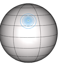
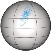
(a) $\boldsymbol{\theta}=(0,0)^{\top}$	(b) $\boldsymbol{\theta}=(-1,-1)^{\top}$
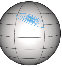
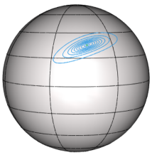
(c) $\boldsymbol{\theta}=(1,1)^{\top}$	(d) $\boldsymbol{\theta}=(-1,1)^{\top}$

Figure 2: Contour plots of the SESPC distribution with $\boldsymbol{\mu}=(5.843,3.057,3.758)^{\top}$ and various $\boldsymbol{\theta}$ parameters.

3.3 Elucidating the Scatter Matrix and Its Role in the SESPC Model

We remind the reader that the scatter matrix $\bm{\Sigma}$ is embedded in (27) via $A={\bf y}^{\top}\boldsymbol{\Sigma}^{-1}\boldsymbol{\mu}$ and $B={\bf y}^{\top}\boldsymbol{\Sigma}^{-1}{\bf y}$, terms which are also included in the term $E$. The largest eigenvalue of the positive definite matrix $\bm{\Sigma}$ $\rho_{3}$ is equal to 1, whilst the other two eigenvalues are $0<\rho_{1}<\rho_{2}$, such that $\rho_{1}\rho_{2}=1$ and the inverse of $\bm{\Sigma}$ can be written as $\bm{\Sigma}^{-1}=\sum_{j=1}^{3}\bm{\xi}_{j}\bm{\xi}_{j}^{\top}/\rho_{j}$, where $\bm{\xi}_{1},\bm{\xi}_{2}$ and $\bm{\xi}_{3}=\bm{\mu}/\gamma$, is a set of mutually orthogonal unit vectors. Note that the third axis, or third eigenvector, is the mean direction, the impact of which is discussed in § 3.4.

As in Paine et al. (2018) we define a pair of unit vectors, $\tilde{\bm{\xi}}_{1}$ and $\tilde{\bm{\xi}}_{2}$, which are orthogonal to each other and to the mean direction $\bm{\xi}_{3}$: $\tilde{\bm{\xi}}_{1}=\left(-\mu_{0}^{2},\mu_{1}\mu_{2},\mu_{1}\mu_{3}\right)^{\top}/(\gamma\mu_{0})$ and $\tilde{\bm{\xi}}_{2}=\left(0,-\mu_{3},\mu_{2}\right)^{\top}/\mu_{0}$, where $\mu_{0}=(\mu_{2}^{2}+\mu_{3}^{2})^{1/2}$. Let us introduce the axes of symmetry $\bm{\xi}_{1}$ and $\bm{\xi}_{2}$ to be an arbitrary rotation of $\tilde{\bm{\xi}}_{1}$ and $\tilde{\bm{\xi}}_{1}$ (Paine et al., 2018), where the relationship between them is given by $\bm{\xi}_{1}=\tilde{\bm{\xi}}_{1}\cos(\psi)+\tilde{\bm{\xi}}_{2}\sin(\psi)$ and $\bm{\xi}_{2}=-\tilde{\bm{\xi}}_{1}\sin(\psi)+\tilde{\bm{\xi}}_{2}\cos(\psi)$, where $\psi$ is the angle of rotation. Let us not denote $\rho=\rho$ and thus $\rho_{2}=1/\rho$, hence we can write the inverse of the scatter matrix as

$$\boldsymbol{\Sigma}^{-1} = \left[\cos^{2}(\psi)/\rho+\rho\sin^{2}(\psi)\right]\tilde{\bm{\xi}}_{1}\tilde{\bm{\xi}}_{1}^{\top}+\left[\sin^{2}(\psi)/\rho+\rho\cos^{2}(\psi)\right]\tilde{\bm{\xi}}_{2}\tilde{\bm{\xi}}_{2}^{\top}$$

$$+0.5\left(1/\rho-\rho\right)\sin(2\psi)\left(\tilde{\bm{\xi}}_{1}\tilde{\bm{\xi}}_{2}^{\top}+\tilde{\bm{\xi}}_{2}\tilde{\bm{\xi}}_{1}^{\top}\right)+\tilde{\bm{\xi}}_{3}\tilde{\bm{\xi}}_{3}^{\top}.$$

Let us now define $\bm{\theta}=\left(\theta_{1},\theta_{2}\right)^{\top}$ such that $\theta_{1}=0.5\left(1/\rho-\rho\right)\cos(2\psi)$ and $\theta_{1}=0.5\left(1/\rho-\rho\right)\sin(2\psi)$, then $\boldsymbol{\Sigma}^{-1}$ becomes

$$\boldsymbol{\Sigma}^{-1}={\bf I}_{3}+\theta_{1}\left(\tilde{\bm{\xi}}_{1}\tilde{\bm{\xi}}_{1}^{\top}-\tilde{\bm{\xi}}_{2}\tilde{\bm{\xi}}_{2}^{\top}\right)+\theta_{2}\left(\tilde{\bm{\xi}}_{1}\tilde{\bm{\xi}}_{2}^{\top}+\tilde{\bm{\xi}}_{2}\tilde{\bm{\xi}}_{1}^{\top}\right)+\left[\left(\theta_{1}^{2}+\theta_{2}^{2}+1\right)^{1/2}-1\right]\left(\tilde{\bm{\xi}}_{1}\tilde{\bm{\xi}}_{1}^{\top}+\tilde{\bm{\xi}}_{2}\tilde{\bm{\xi}}_{2}^{\top}\right).$$

The use of the $\tilde{\bm{\xi}}_{i}$s axes allows for unconstrained parameter estimation, since, unlike the eigenvalues of $\bm{\Sigma}$, $\theta_{1}$ and $\theta_{2}$ lie on the real line. Further, note that the total number of free parameters is five, the same as for the bivariate Cauchy distribution in a tangent space $\mathbb{R}^{2}$ to the sphere.

If $\boldsymbol{\theta}={(0,0)^{\top}}$ then $\bm{\Sigma}={\bf I}_{3}$ and hence (27) reduces to (26) yielding rotational symmetry. The rotational symmetry can, hence, be tested using the log-likelihood ratio test which, under the null hypothesis, asymptotically follows a $\chi^{2}$ distribution with two degrees of freedom. Rejection of the rotational symmetry favors the SESPC model (27) over the SIPC model (26). Non-parametric bootstrap is an alternative, especially in cases where the sample size is not sufficiently large to allow for the asymptotic null distribution to be valid.

3.4 Examining the Influence of the Mean Direction as an Eigenvector

The first condition imposed was that $\bm{\Sigma}\bm{\mu}=\bm{\mu}$, indicating that the second eigenvector (i.e., the eigenvector corresponding to the second highest eigenvalue $\rho_{2}=1$) is equal to the mean direction $\bm{\mu}/\gamma$. As Paine et al. (2018) assert, this condition enforces symmetry about the eigenvectors of $\boldsymbol{\Sigma}$. Without loss of generality, assume that the eigenvectors are parallel to the coordinate axes; in other words, each element of the vector $\bm{\xi}_{j}$ is equal to 0 except for the $j$-th element, which is equal to 1. Then, if ${\bf y}=\left(y_{1},y_{2},y_{3}\right)^{\top}$,

$${\bf y}^{\top}\bm{\xi}_{3}=y_{3}\ \ \text{and}\ \ {\bf y}^{\top}\bm{\Sigma}^{-1}{\bf y}=y_{3}^{2}+\sum{j=1}^{2}y^{2}_{j}/\rho_{j}.$$ (28)

In this situation, the density in (27) depends solely on $y_{j}$ through $y_{j}^{2}$ for $j=1,2$. As a result, the density remains invariant with respect to the sign changes of $y_{1},y_{2}$, that is, $f_{SESPC}(\pm y_{1},\pm y_{2},y_{3})=f_{SESPC}(y_{1},y_{2},y_{3})$, implying reflective symmetry about 0 along the axes defined by $\bm{\xi}_{1}$ and $\bm{\xi}_{2}$. This type of symmetry is suggested by ellipse-like contours of constant density inscribed on the sphere, and such contours arise when the density (7) is unimodal. Whether the density is unimodal depends on the nature of the stationary point at ${\bf y}=\bm{\mu}/\gamma$.

Proposition 1

The SESPC has a global maximum at ${\bf y}=\bm{\xi}_{3}=\bm{\mu}/\gamma$.

A rigorous proof seems challenging, and our conjecture is that if the stationary point is a local maximum, it must also be a global maximum, leading to a unimodal distribution. This conjecture is strongly supported by the extensive numerical investigations we have conducted. Assume without loss of generality that $\bm{\mu}=\gamma(0,0,1)^{\top}$, and therefore $\bm{\xi}_{3}=(0,0,1)^{\top}$. This implies that ${\bf\xi}_{1}=(1,0,0)^{\top}$ and ${\bf\xi}_{2}=(0,1,0)^{\top}$. Following Paine et al. (2018), let us write ${\bf y}=\left(0,u,\left(1-u^{2}\right)^{1/2}\right)^{\top}$ and focus on $u$, which lies in a neighborhood of 0. By substituting ${\bf y}$ into the logarithm of (27) and by differentiating this and setting it equal to zero, we arrive at $\frac{\partial\log{f(u)}}{\partial u}\Big{|}_{u=0}=0$. The second derivative must then be negative: $\frac{\partial^{2}\log{f(u)}}{\partial u^{2}}\Big{|}_{u=0}<0$. For a range of values of $\gamma$ from 1 up to 10, and a range of values for $\rho_{2}$ from 0.01 up to 0.99, both in increments of 0.01, we computed the second derivative. The second derivative was consistently negative for all combinations of $\gamma$ and $\rho_{2}$ values. This empirical evidence strongly supports the conjecture that the SESPC has a global maximum at ${\bf y}=\bm{\xi}_{3}=\bm{\mu}/\gamma$, suggesting that the distribution is unimodal under these conditions.

3.5 Spherical Regression

In this section, we adopt the second parameterisation (structure 2) as presented by Paine et al. (2018) to establish a connection between the mean direction $\bm{\mu}$ and covariates ${\bf X}$. The approach closely resembles that of circular regression, with $\bm{\mu}_{i}=\left(\bm{\beta}_{1}^{\top}{\bf x}_{i},\bm{\beta}_{2}^{\top}{\bf x}_{i},\bm{\beta}_{3}^{\top}{\bf x}_{i}\right)^{\top}={\bf B}^{\top}{\bf x}_{i}$. The key distinction from circular regression lies in the fact that ${\bf Qy}_{i}\sim\text{SESPC}\left({\bf B}^{\top}{\bf x}_{i},\bm{\theta}\right)$, where ${\bf Q}\in\textit{O}(3)$ is an estimable rotation matrix. To maximise the associated regression log-likelihood, we optimise with respect to $\bf Q$, $\bf B$, and $\boldsymbol{\theta}$.

To achieve this, a grid search is performed over the orthogonal group, $\textit{O}(3)$. For each value of $\bf Q$, the response variable ${\bf y}$ is rotated, and the log-likelihood is maximised. The log-likelihood-maximising value of $\bf Q$ is chosen, and the corresponding regression coefficients and $\bm{\theta}$ values are reported.

The log-likelihood ratio test can be employed to test for rotational symmetry (or isotropy) when $\bm{\theta}=(0,0)^{\top}$, as well as for assessing the significance of one or more covariates. For cases with small sample sizes, the non-parametric bootstrap approach can be considered as an alternative.

4 Simulation Studies

The conducted simulation studies comprehensively address the aspects delineated earlier, including an exploration of particular properties pertaining to the maximum likelihood estimation for circular and spherical models, both in the presence and absence of covariates. Furthermore, we draw comparisons between these models and a selection of well-known distributions in the literature.

4.1 Comparison of CIPC and GCPC Models

Initially, we evaluate the bias in the estimated mean vector when the data are generated from the GCPC model with a mean vector equal to $\bm{\mu}=(3,10)^{\top}$ and $\rho=(0.1,0.3,0.5,0.7,0.7,1)$ for various sample sizes, $n=(50,100,300,500,1000)$. The objectives of this study are: a) to assess the bias of the estimated mean vector between the two models, CIPC and GCPC, and b) to evaluate the power of the log-likelihood ratio in discriminating between the two models. The log-likelihood ratio test statistic in this case follows a mixture of Dirac distribution at 1 and a $\chi^{2}_{1}$ distribution with a mixing probability of 0.5.

Table 1 presents the Euclidean distances of the estimated mean vectors under the CIPC and GCPC models, averaged over 1,000 repetitions. It also provides the estimated power for testing whether $\rho=1$, i.e., distinguishing between the two models. The results clearly demonstrate that when $\rho<<1$, the accuracy of the GCPC model is considerably higher than that of the CIPC model. Furthermore, the discrepancy between them increases with the sample size. As $\rho$ approaches $1$, the differences diminish; when $\rho=0.9$ and $\rho=1$, the Euclidean distance of the estimated mean vector under the GCPC model is greater than that under the CIPC model. We attribute this phenomenon to the small proportion of times that the log-likelihood ratio rejects the CIPC in favor of the GCPC. To validate this, we computed the averages excluding these cases and observed that the average Euclidean distances were almost identical.

Table 1: Average Euclidean distances between the true mean vector $\boldsymbol{\mu}=(3,10)^{\top}$ and the estimated mean vector using CIPC and GCPC distributions for various $\rho$ values and sample sizes. The row termed Power contains the estimated power for testing whether $\rho=1$ (when $\rho=1$, the GCPC reduces to the CIPC model).

		Sample size
$\rho$	Model and Power	n=50	n=100	n=300	n=500	n=1000
$\rho=0.1$	CIPC	23.467	23.043	22.824	22.505	22.470
	GCPC	9.856	6.343	2.924	2.226	1.688
	Power	0.438	0.633	0.942	0.983	0.985
$\rho=0.3$	CIPC	9.337	8.874	8.646	8.612	8.589
	GCPC	5.762	4.475	2.655	2.026	1.355
	Power	0.231	0.345	0.622	0.819	0.960
$\rho=0.5$	CIPC	5.028	4.485	4.363	4.392	4.299
	GCPC	3.995	3.134	2.181	1.778	1.309
	Power	0.125	0.180	0.367	0.503	0.732
$\rho=0.7$	CIPC	3.014	2.388	2.096	2.117	2.054
	GCPC	2.983	2.306	1.725	1.491	1.171
	Power	0.091	0.100	0.197	0.236	0.355
$\rho=0.9$	CIPC	1.990	1.373	0.884	0.743	0.615
	GCPC	2.587	1.980	1.272	1.039	0.826
	Power	0.051	0.061	0.082	0.094	0.114
$\rho=1$	CIPC	1.761	1.207	0.682	0.543	0.378
	GCPC	2.372	1.923	1.095	0.964	0.715
	Power	0.049	0.057	0.049	0.057	0.058

4.2 Comparison of GCPC, CIPC, and SPML Regression Models

We examine the bias of the estimated coefficients in a regression setting with a single covariate for the sake of simplicity. The matrix of regression coefficients is defined as

$${\bf B}=(\bm{\beta}_{1}^{T},\bm{\beta}_{2}^{T})^{T}=\left(\begin{array}[]{cc}-0.2831&-0.892\\ 0.066&0.090\end{array}\right),$$

where the first row corresponds to the constant terms, and the second row represents the slopes. The two columns correspond to $\cos(\theta)$ and $\sin(\theta)$.

The covariate $X$ was generated from a $Ga(2.590,0.054)$ distribution, and then values of $\theta$ were generated from the GCPC model with a mean vector equal to $\mu_{i}=\left(\bm{\beta}_{1}{\bf x}_{i},\bm{\beta}_{2}{\bf x}_{i}\right)^{\top}$ and $\rho=(0.1,0.3,0.5,0.7,0.7,1)$ for various sample sizes, $n=(50,100,300,500,1000)$. The objective of this study is to evaluate the bias of the estimated matrix of regression coefficients among the SPML, CIPC, and GCPC regression models. The bias was calculated using the Frobenius norm, $|\hat{\bf B}-{\bf B}|_{F}$.

Table 2 presents the Frobenius norms of the regression coefficients estimated using the SPML, CIPC, and GCPC regression models, averaged over 1,000 repetitions. The estimated bias of the SPML model remains constant irrespective of the sample size and the value of $\rho$. In contrast, the GCPC and CIPC models are influenced by the sample size. As the sample size increases, their bias decreases. In the intra-comparison, the bias of the CIPC model is considerably larger than that of the GCPC model for small values of $\rho$. As $\rho$ grows, the GCPC model approaches the CIPC model, and the biases become similar.

Table 2: Average Frobenius norm between the true and the estimated regression coefficients using SPML, CIPC, and GCPC regression models for various $\rho$ values and sample sizes.

		Sample size
$\rho$	Model	n=50	n=100	n=300	n=500	n=1000
$\rho=0.1$	SPML	1.135	1.104	1.190	1.204	1.207
	CIPC	7.053	6.497	6.211	6.189	6.162
	CESPC	2.254	1.595	1.138	1.111	0.942
$\rho=0.3$	SPML	1.324	1.376	1.429	1.447	1.446
	CIPC	2.962	2.610	2.419	2.358	2.348
	CESPC	1.374	0.977	0.547	0.458	0.318
$\rho=0.5$	SPML	1.455	1.516	1.558	1.560	1.574
	CIPC	1.764	1.461	1.255	1.213	1.190
	CESPC	1.165	0.824	0.508	0.381	0.283
$\rho=0.7$	SPML	1.550	1.606	1.632	1.651	1.661
	CIPC	1.292	0.914	0.659	0.612	0.574
	CESPC	1.082	0.744	0.447	0.356	0.256
$\rho=0.9$	SPML	1.620	1.675	1.695	1.704	1.721
	CIPC	1.041	0.673	0.402	0.321	0.238
	CESPC	1.003	0.657	0.405	0.322	0.233
$\rho=1.0$	SPML	1.634	1.687	1.729	1.736	1.741
	CIPC	1.023	0.628	0.350	0.275	0.190
	CESPC	0.995	0.665	0.388	0.299	0.215

4.3 Comparison of SIPC and SESPC Models

We investigate the bias in the estimated mean vector when the data are generated from the SESPC model with a mean vector equal to $\boldsymbol{\mu}=c(5.843,3.057,3.758)^{\top}$ and $\theta_{1}=\theta_{2}=(0.1,0.3,0.5,0.7,0.7,1)$ for various sample sizes, $n=(50,100,300,500,1000)$. The objectives of this study are to: a) evaluate the bias of the estimated mean vector between the SIPC and SESPC models, and b) assess the power of the log-likelihood ratio in discriminating between the two models.

Table 3 presents the Euclidean distances of the estimated mean vectors under the SIPC and SESPC models, averaged over 1,000 repetitions. Additionally, the table includes the estimated power for testing whether $\theta_{1}=\theta_{2}=0$, i.e., discriminating between the two models. The results clearly demonstrate that as the $\theta$ values increase, the accuracy of the SESPC model becomes significantly higher than that of the SIPC model. Moreover, the discrepancy between the two models increases with the sample size. As expected, as the $\theta$ values approach 0, the differences between the models diminish.

Table 3: Average Euclidean distances between the true mean vector is $\boldsymbol{\mu}=(5.843,3.057,3.758)^{\top}$ and the estimated mean vector $\hat{\boldsymbol{\mu}}$ using SIPC and SESPC distributions for various values of common $\theta$ parameters. The row termed Power contains the estimated power for testing rotational symmetry ($\theta_{1}=\theta_{2}=0$), i.e., the SIPC distribution versus the SESPC distribution.

		Sample size
$(\theta_{1},\theta_{2})$	Model and Power	n=50	n=100	n=300	n=500	n=1000
$\theta_{1}=\theta_{2}=0$	SIPC	1.106	0.739	0.422	0.332	0.221
	SESPC	1.123	0.747	0.424	0.334	0.222
	Power	0.057	0.060	0.065	0.049	0.050
$\theta_{1}=\theta_{2}=0.2$	SIPC	1.082	0.740	0.426	0.331	0.243
	SESPC	1.111	0.755	0.429	0.329	0.237
	Power	0.249	0.477	0.930	0.991	1.000
$\theta_{1}=\theta_{2}=0.4$	SIPC	1.057	0.765	0.450	0.373	0.309
	SESPC	1.151	0.778	0.430	0.327	0.234
	Power	0.764	0.968	1.000	1.000	1.000
$\theta_{1}=\theta_{2}=0.6$	SIPC	1.071	0.819	0.552	0.498	0.465
	SESPC	1.100	0.776	0.429	0.336	0.233
	Power	0.959	1.000	1.000	1.000	1.000
$\theta_{1}=\theta_{2}=0.8$	SIPC	1.133	0.886	0.736	0.730	0.726
	SESPC	1.206	0.765	0.425	0.339	0.242
	Power	0.988	0.999	1.000	1.000	1.000
$\theta_{1}=\theta_{2}=1$	SIPC	1.226	1.022	0.997	0.970	0.985
	SESPC	1.258	0.843	0.433	0.327	0.241
	Power	0.981	0.993	1.000	1.000	0.999

4.4 Comparative Analysis of SESPC, SIPC, and SC Models

We evaluate the accuracy of the SESPC, SIPC, and SC models in estimating the mean direction of the fitted model, $\widehat{\bf m}=\widehat{\boldsymbol{\mu}}/\hat{\gamma}$, under the conditions where the data are generated using the SESPC model for a range of $\theta_{1}$ and $\theta_{2}$ values. The measure employed for this analysis is $\sqrt{2\left[1-\text{E}\left(\widehat{\bf m}^{\top}\hat{\bf m}\right)\right]}$, with the expectation approximated by Monte Carlo.

Table 4 presents the following quantity:

$$\text{Error}\left(\widehat{\bf m}\right)=\sqrt{2\left[1-B^{-1}\sum_{b=1}^{B}\left(\widehat{\bf m}_{i}^{\top}{\bf m}\right)\right]},$$

where $\left(\widehat{\bf m}_{i}\right)$ represents the estimated mean direction of the fitted model for the $i$-run out of $B$ Monte Carlo runs. Regardless of the $\theta_{s}$ values, the errors for SESPC and SIPC are nearly identical for large sample sizes ($n\geq 300$), suggesting that SIPC performs well in estimating the mean direction even when elliptical symmetry exists. It is important to note, however, that this observation does not apply to the estimated concentration parameters, $\hat{\gamma}$ (not presented).

Table 4: The $\text{Error}\left(\widehat{\bf m}\right)$ of the fitted model when the true mean vector is $\boldsymbol{\mu}=(5.843,3.057,3.758)^{\top}$ and hence the true mean direction is ${\bf m}=(0.770,0.403,0.495)^{\top}$.

		Sample size
$(\theta_{1},\theta_{2})$	$\text{Error}\left(\widehat{\bf m}\right)$	n=50	n=100	n=300	n=500	n=1000
$\theta_{1}=\theta_{2}=0$	SC	0.151	0.139	0.151	0.162	0.147
	SIPC	0.035	0.024	0.014	0.011	0.008
	SESPC	0.035	0.024	0.014	0.011	0.008
$\theta_{1}=\theta_{2}=0.2$	SC	0.136	0.158	0.128	0.162	0.159
	SIPC	0.036	0.026	0.014	0.011	0.008
	SESPC	0.036	0.026	0.014	0.011	0.008
$\theta_{1}=\theta_{2}=0.4$	SIPC	0.038	0.027	0.015	0.012	0.008
	SC	0.156	0.137	0.143	0.159	0.150
	SESPC	0.095	0.051	0.015	0.012	0.046
$\theta_{1}=\theta_{2}=0.6$	SC	0.149	0.152	0.147	0.104	0.138
	SIPC	0.043	0.030	0.017	0.012	0.009
	SESPC	0.109	0.029	0.017	0.012	0.063
$\theta_{1}=\theta_{2}=0.8$	SC	0.160	0.161	0.160	0.153	0.151
	SIPC	0.045	0.031	0.018	0.014	0.010
	SESPC	0.193	0.067	0.017	0.013	0.046
$\theta_{1}=\theta_{2}=1$	SC	0.177	0.151	0.141	0.135	0.147
	SIPC	0.053	0.034	0.020	0.015	0.011
	SESPC	0.241	0.111	0.019	0.014	0.010

4.5 Evaluation of SESPC and SIPC Regression Models

We generated data from a single-covariate regression model, with the matrix of coefficients being defined as:

$${\bf B}=\left(\begin{array}[]{ccc}-1&1&-0.5\\ 0.4&-0.5&0.3\end{array}\right),$$

where the first row represents the constant term, and the second row corresponds to the slope. The data were generated from the SESPC model with $\theta_{1}=\theta_{2}=0$ (corresponding to the SIPC model) and with $\theta_{1}=-2$ and $\theta_{2}=2$ for various sample sizes. We estimated the regression model using both SIPC and SESPC (without applying the rotation matrix $\bf Q$) and computed the Frobenius norm between the true and estimated regression coefficient matrices. Table 5 displays the average norms over 1,000 iterations.

Under isotropy conditions (SIPC model), the results between the two regression models are comparable. However, when the $\theta$ parameters are non-zero, differences in the estimated bias of the regression coefficients become apparent.

Table 5: Average Frobenius norm between the true and the estimated regression coefficients using SIPC, and SESPC regression models for various sample sizes.

		Sample size
$(\theta_{1},\theta_{2})$	Model	n=50	n=100	n=300	n=500	n=1000
$\theta_{1}=\theta_{2}=0$	SIPC	0.805	0.509	0.285	0.215	0.151
	SESPC	0.892	0.570	0.295	0.221	0.155
$\theta_{1}=-2,\ \theta_{2}=2$	SIPC	1.237	0.846	0.630	0.563	0.518
	SESPC	0.889	0.714	0.549	0.535	0.474

5 Empirical Illustrations with Real Data: A Comparative Analysis

In this section, we present a series of real-world data examples to demonstrate the effectiveness and advantages of our proposed models. Through these empirical illustrations, we aim to provide a comparative analysis that highlights the superior performance of the suggested models over some of the prevalent models in the field. This comprehensive comparison serves to emphasise the practical applicability and relevance of our newly developed models in addressing real-world problems and challenges.

5.1 Circular Data without Covariates

The first example pertains to a dataset that comprises measurements of the directions taken by 76 turtles after undergoing a specific treatment (Fisher, 1995, pg. 241). We present the estimated parameters of the CIPC and GCPC models in Table 6. In general, the parameters appear to be quite similar, except for the $\gamma$ parameter for the CIPC model, which exhibits a higher value. The p-value for the hypothesis that $\rho=1$ is equal to 0.0002, indicating a clear preference for the GCPC model over the CIPC model. Figure 3 displays the kernel density estimate of the data alongside the fitted densities of the CIPC and the GCPC models. Both the CIPC and GCPC models produce a higher density for the first mode; however, only the GCPC model is successful in capturing the second mode. This result emphasises the superior performance of the GCPC model in this particular example.

Table 6: Estimated parameters for the CIPC and GCPC models for the Turtles dataset.

Model	$\hat{\mu}$	$\hat{\bm{\mu}}$ in $\hat{\mathbb{S}^{1}}$	$\hat{\bm{\mu}}$ in $\mathbb{R}^{2}$	$\hat{\gamma}$	$\hat{\rho}$	Log-likelihood
CIPC	1.107	$(0.448,0.894)^{\top}$	$(0.730,1.458)^{\top}$	1.630		-113.248
GCPC	1.094	$(0.459,0.889)^{\top}$	$(0.458,0.888)^{\top}$	0.999	0.341	-109.857

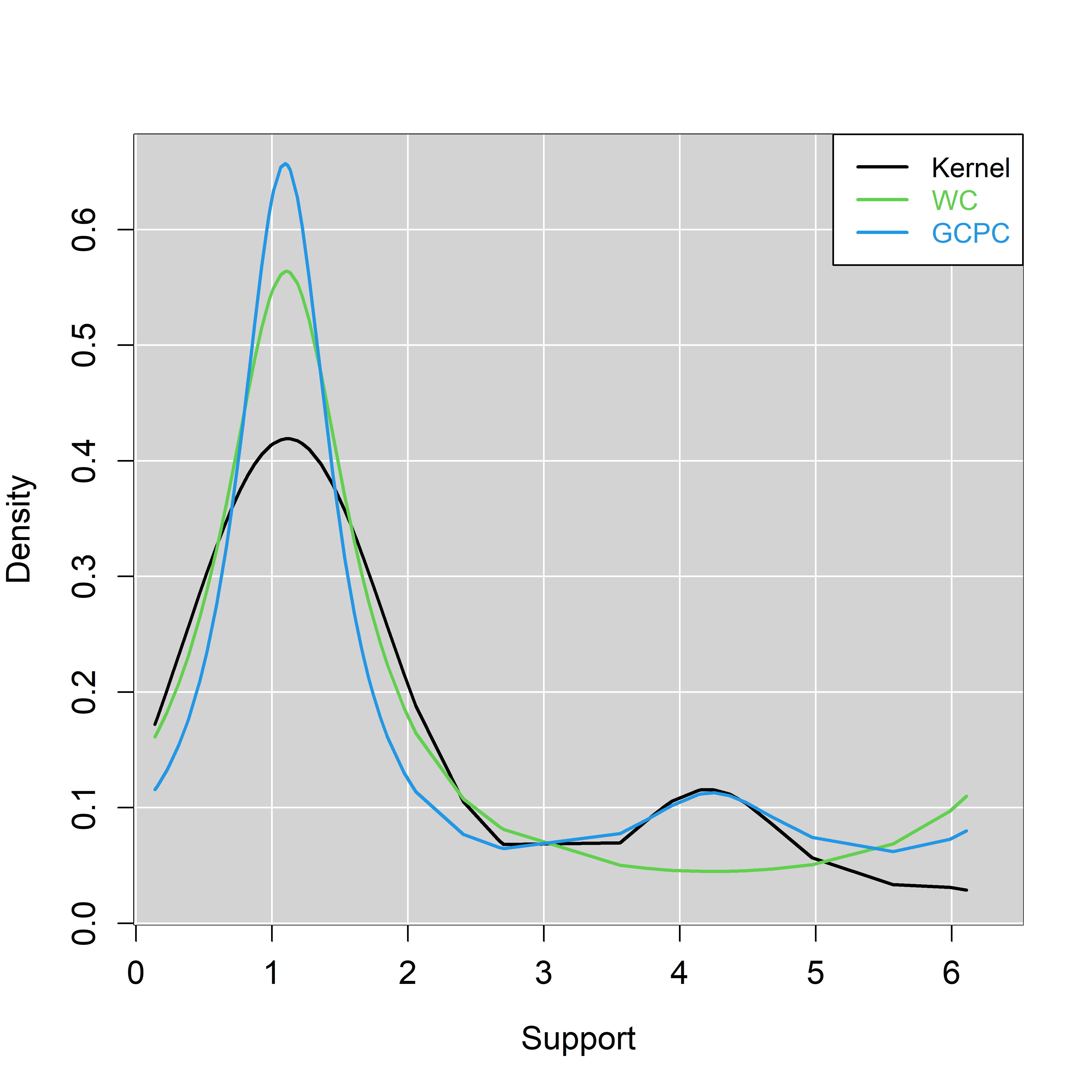
Figure 3: The kernel density estimate, and the WC & GCPC densities of the turtles dataset.

5.2 Circular Data with Covariates

The second example explores the regression setting using wind data. The dataset contains hourly observations of wind direction and wind speed during the winter season (from November to February) from 2003 until 2012 on the Atlantic coast of Galicia (NW–Spain). Data are recorded by a buoy located at longitude -0.21^∘ east and latitude 43.5^∘ north in the Atlantic Ocean. However, due to the time series nature of the data, only a subset of 200 points was analysed. This dataset, as analysed in Oliveira, Crujeiras and Rodríguez-Casal (2014), was obtained by selecting observations with a lag period of 95 hours.

Table 7 presents the estimated regression parameters using the PN, CIPC, and GCPC distributions for the fitted regression models. The log-likelihood values for the CIPC and GCPC regression models were found to be $-363.370$ and $-334.732$, respectively. Furthermore, the $\rho$ parameter of the GCPC distribution was estimated to be 0.222 with a standard error of 0.044. The circular correlation coefficient (Mardia and Jupp, 2000) between the observed and fitted angular data is equal to $0.044,0.042$, and $0.080$ for the SPML, CIPC, and GCPC regression models, respectively.

Table 7: Estimated regression parameters (their standard errors appear within parentheses) for the PN, CIPC, and GCPC regression models fitted to the wind data.

Model	PN		CIPC		GCPC
	$\cos(y)$	$\sin(y)$	$\cos(y)$	$\sin(y)$	$\cos(y)$	$\sin(y)$
$\hat{\bm{\alpha}}$	0.333(0.185)	0.120(0.181)	0.458(0.282)	0.209(0.245)	-0.042 (0.0013)	-0.045(0.0023)
$\hat{\bm{\beta}}$	-0.024(0.021)	-0.007(0.020)	-0.033(0.032)	-0.011(0.028)	0.009(0.0005)	0.010(0.0009)
	Loglik	$\hat{\rho}$	Loglik	$\hat{\rho}$	Loglik	$\hat{\rho}$
	-363.893	-	-363.370	-	-331.846	0.203(0.039)

5.3 Comparative Analysis of Spherical Data Distributions Without Covariates

We visually compared the density values of the SIPC, SESPC, and spherical Cauchy distributions using the Paleomagnetic pole dataset (Schmidt, 1976). This dataset comprises estimates of the Earth’s historical magnetic pole position calculated from 33 distinct sites in Tasmania. The data are illustrated in Figure 4. Notably, rotational symmetry is rejected (p-value = 0.0026), supporting the findings of Paine et al. (2018).

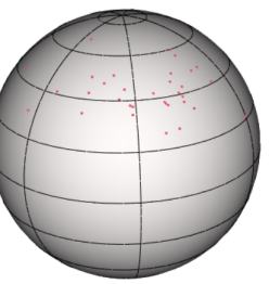
Figure 4: Sphere plot of the Paleomagnetic dataset.

Table 8 presents the estimated parameters for each of the three distributions. The mean directions are evidently close to one another. Figure 5 displays the spherical contour plots of the fitted densities, revealing that SESPC has more accurately captured the data’s shape.

Figure 6 showcases the transects of the densities of the three distributions. We computed the density values for 1,000 latitude and longitude values within the observed data range. We matched the latitude to the mean direction latitude of the SESPC distribution and allowed the longitude to vary. Consequently, Figure 6 displays a slice of the multivariate density as a function of longitude when the latitude is $134.71^{\circ}$.

Table 8: Estimated parameters for the SIPC, SESPC, and SC distributions. The columns present the estimated mean direction in Euclidean and polar coordinates, the estimated concentration parameters, and the estimated $\theta$ parameters for the SESPC.

Model	Estimated parameters
Spherical Cauchy	$\hat{\bm{\mu}}=(-0.699,0.224,0.679)^{\top}$	$\hat{\bm{\mu}}=(134.36^{\circ},71.75^{\circ})^{\top}$	$\hat{\rho}=0.752$
SIPC	$\hat{\bm{\mu}}=(-4.155,1.130,3.834)^{\top}$	$\hat{\bm{\mu}}=(136.11^{\circ},73.58^{\circ})^{\top}$	$\hat{\gamma}=5.766$
SESPC	$\hat{\bm{\mu}}=(-4.207,1.433,3.991)^{\top}$	$\hat{\bm{\mu}}=(134.77^{\circ},70.25^{\circ})^{\top}$	$\hat{\gamma}=5.973$	$\hat{\boldsymbol{\theta}}=(0.219,-0.846)^{\top}$

The rotational symmetry assumption is rejected (p-value=0.0026), resulting in similar densities for the SIPC and SESPC, as anticipated. The densities differ, with their shapes being alike but the locations of the modes being slightly different, illustrating the effect of the elliptical symmetry present in the data.

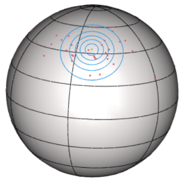
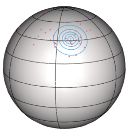
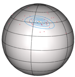
(a) Spherical Cauchy	(b) SIPC	(c) SESPC

Figure 5: Comparison of the three distributions fitted to the Paleomagnetic dataset: spherical contour plots of each fitted distribution.

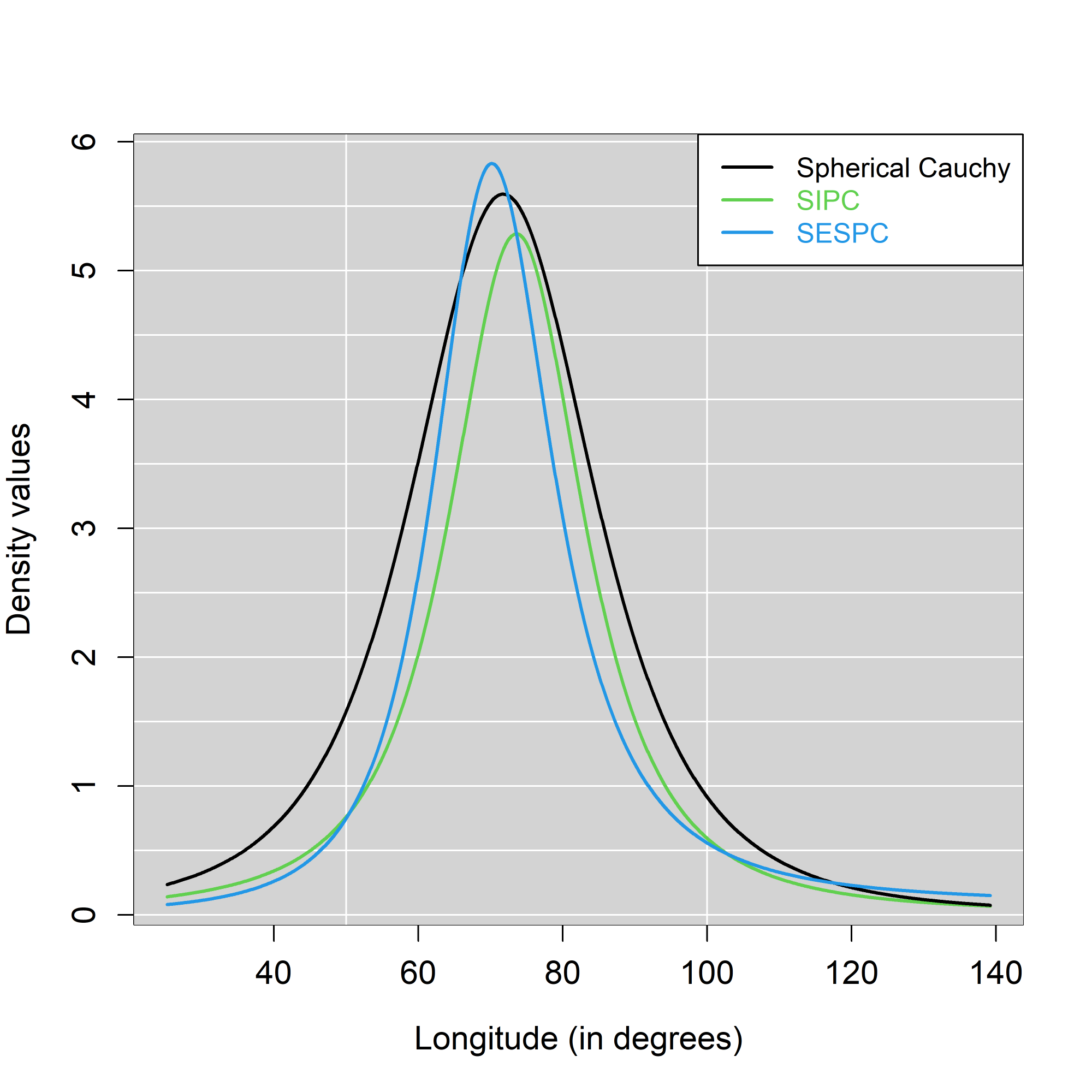
Figure 6: Comparison of the three distributions fitted to the Paleomagnetic dataset: transects of the densities when Latitude=$134.71^{\circ}$.

5.4 Comparative Analysis of Spherical Data Distributions with Covariates

The data used in this analysis are sourced from vectorcardiogram measurements of children’s heart electrical activity, taking into account different ages and genders (Downs, Liebam and Mackay, 1971). Vectorcardiograms involve attaching three leads to the torso, producing a time-dependent vector that traces approximately closed curves, with each curve representing a heartbeat cycle in $\mathbb{R}^{3}$. A unit vector, defined as the directional component of the vector at a particular extremum across the cycles, is sometimes employed as a clinical diagnostic summary.

The dataset consists of unit vectors derived from two different lead placement systems: the McFee system (${\bf y}_{i}\in\mathbb{S}^{2}$) and the Frank system (${\bf u}_{i}\in\mathbb{S}^{2}$) for each of 98 children from different age groups ($A_{i}$) and genders ($G_{i}$) , with $i=1,\ldots,98$. We regressed the McFee system (${\bf y}$) on the Frank system (${\bf u}$), age ($A$), and gender ($G$) using the SIPC and SESPC. Table 9 presents the estimated regression parameters for each of the two models.

The log-likelihood values for the SIPC and SESPC regression models are 40.134 and 233.466, respectively. Evidently, the isotropy assumption of the SIPC regression model is rejected. This finding is consistent with the results of Paine et al. (2020), who also rejected the isotropy assumption of the Gaussian distribution.

Table 9: Estimated regression parameters (their standard errors appear within parentheses) for the SIPC and SESPC regression models.

	SISPC			SESPC
Variables	$Y_{1}$	$Y_{2}$	$Y_{3}$	$Y_{1}$	$Y_{2}$	$Y_{3}$
Constant	-2.265(1.407)	-1.457(1.445)	-1.974(2.798)	-0.525(1.327)	2.483(2.747)	1.002(1.722)
Age	0.667(0.585)	0.791(0.685)	0.274(0.650)	0.417(0.468)	-0.648(0.814)	-0.451(0.468)
Sex	1.608(0.701)	0.860(0.703)	0.483(0.731)	0.215(0.483)	-1.072(0.943)	-1.365(0.508)
MQRS1	8.495(1.454)	0.282(1.060)	2.660(2.126)	-2.320(0.933)	-7.100(1.882)	-4.674(1.551)
MQRS2	-2.535(1.217)	9.183(1.857)	5.540(2.196)	10.503(1.725)	-4.417(2.130)	1.527(1.484)
MQRS3	0.457(0.573)	1.024(0.640)	7.553(1.191)	1.566(0.451)	-6.696(1.089)	3.987(0.798)

6 Conclusions

In this study, we introduced the projected Cauchy distribution on both the circle and the sphere. For the circular case, projecting the bivariate Cauchy distribution resulted in the wrapped Cauchy distribution with an improved parameterisation. We then devised a generalised projected Cauchy distribution by imposing a restriction on the scatter matrix, thus adding an extra parameter. We emphasise that exploring alternative scatter matrix structures could also be valuable. Through simulation studies and real data analysis, we demonstrated that the GCPC distribution offers a superior alternative to the WC distribution, irrespective of covariate presence.

In the spherical case, we used a similar strategy by projecting the trivariate Cauchy distribution onto the sphere and imposing two conditions on the scatter matrix, achieving elliptical symmetry. Despite the limitations of an inconvenient density formula and challenges in generalising the density formula to higher dimensions, the projected Cauchy family of distributions provides key advantages. These benefits include a closed-form normalising constant and an efficient method for simulating values, as well as being one of the few elliptically symmetric distributions on the sphere. The proposed distributions have not been fully explored, and there are several opportunities for future research. For example, comparing the GCPC distribution with other variants derived from the projected Cauchy distribution and other three-parameter circular distributions would be valuable. Additionally, pursuing Bayesian estimation of the PC distribution, following the approaches in Wang and Gelfand (2013) and Hernandez-Stumpfhauser and Breidt and van der Woerd (2017), could provide new insights.

Appendix

A1 Derivation of (3)

We recall the terms used, $A={\bf y}^{\top}\boldsymbol{\Sigma}^{-1}\boldsymbol{\mu}$, $B={\bf y}^{\top}\boldsymbol{\Sigma}^{-1}{\bf y}$ and $\Gamma^{2}=\boldsymbol{\mu}^{\top}\boldsymbol{\Sigma}^{-1}\boldsymbol{\mu}$. Thus, the indefinite integral above Eq. (3), which we will solve in the first place, can be written as

$$I = \int\frac{r}{\left(1+Br^{2}-2Ar+\Gamma^{2}\right)^{3/2}}dr$$ (A1.1)

$$= \int\left(\frac{Br-A}{B\left(Br^{2}-2Ar+\Gamma^{2}+1\right)^{3/2}}+\frac{A}{B\left(Br^{2}-2Ar+\Gamma^{2}+1\right)^{3/2}}\right)dr$$ (A1.2)

$$= \frac{1}{B}\int\frac{Br-A}{\left(Br^{2}-2Ar+\Gamma^{2}+1\right)^{3/2}}dr+\frac{A}{B}\int\frac{1}{\left(Br^{2}-2Ar+\Gamma^{2}+1\right)^{3/2}}dr=\frac{1}{B}I_{1}+\frac{A}{B}I_{2}$$ (A1.3)

Let us now solve the first integral ($I_{1}$). Substitute $u=Br^{2}-2Ar+\Gamma^{2}+1$ and thus $du=2(Br-A)dr$, hence the first integral becomes

$$I_{1}=\frac{1}{2}\int\frac{1}{u^{3/2}}du=-\frac{1}{\sqrt{u}}=-\frac{1}{\sqrt{Br^{2}-2Ar+\Gamma^{2}+1}}.$$ (A1.5)

Let us now solve the second integral ($I_{2}$).

$$I_{2}=B^{3/2}\int\frac{1}{\left[\left(Br-A\right)^{2}+B\left(\Gamma^{2}+1\right)-A^{2}\right]^{3/2}}dr=B^{3/2}I_{3}.$$ (A1.6)

Substitute $u=Br-A$ and hence $du=Bdr$, thus $I_{3}$ can be written as

$$I_{3}=\frac{1}{B}\int\frac{1}{\left[u^{2}+B\left(\Gamma^{2}+1\right)-A^{2}\right]^{3/2}}du=\frac{1}{B}I_{4}.$$ (A1.7)

Again, using substitution, $u=\sqrt{B\left(\Gamma^{2}+1\right)-A^{2}}\tan(v)$ and $v=\arctan\left(\frac{u}{\sqrt{B\left(\Gamma^{2}+1\right)-A^{2}}}\right)$. Then
$du=\sqrt{B\left(\Gamma^{2}+1\right)-A^{2}}\sec^{2}(v)dv$. Thus, $I_{4}$ becomes

$$I_{4} = \int\frac{\sqrt{B\left(\Gamma^{2}+1\right)-A^{2}}\sec^{2}(v)}{\left[\left(B\left(\Gamma^{2}+1\right)-A^{2}\right)\tan^{2}(v)+B\left(\Gamma^{2}+1\right)-A^{2}\right]^{3/2}}dv=\frac{1}{B\Gamma^{2}+B-A^{2}}\int\frac{1}{sec(v)}dv$$ (A1.8)

$$= \frac{sin(v)}{B\Gamma^{2}+B-A^{2}}.$$ (A1.9)

We undo the last substitution, and hence $\sin(v)=\sin\left[\arctan\left(\frac{u}{\sqrt{B\left(\Gamma^{2}+1\right)-A^{2}}}\right)\right]=\frac{u}{\sqrt{B\left(\Gamma^{2}+1\right)-A^{2}}\sqrt{\frac{u^{2}}{\sqrt{B\left(\Gamma^{2}+1\right)-A^{2}}}+1}}$. We plug this last result into $I_{4}$ to obtain

$$I_{4}=\frac{u}{\left(B\Gamma^{2}+B-A^{2}\right)\sqrt{B\left(\Gamma^{2}+1\right)-A^{2}}\sqrt{\frac{u^{2}}{\sqrt{B\left(\Gamma^{2}+1\right)-A^{2}}}+1}}$$ (A1.10)

and hence $I_{3}$ becomes

$$I_{3}=\frac{u}{B\left(B\Gamma^{2}+B-A^{2}\right)\sqrt{B\left(\Gamma^{2}+1\right)-A^{2}}\sqrt{\frac{u^{2}}{\sqrt{B\left(\Gamma^{2}+1\right)-A^{2}}}+1}}.$$ (A1.11)

We now undo the substitution that took us from $I_{2}$ to $I_{3}$ and obtain

$$I_{2}=\frac{B^{3/2}\left(Br-A\right)}{B\left(B\Gamma^{2}+B-A^{2}\right)\sqrt{B\left(\Gamma^{2}+1\right)-A^{2}}\sqrt{\frac{\left(Br-A\right)^{2}}{\sqrt{B\left(\Gamma^{2}+1\right)-A^{2}}}+1}}.$$ (A1.12)

Finally, $I$ is written as

$$I=-\frac{1}{B}\frac{1}{\sqrt{Br^{2}-2Ar+\Gamma^{2}+1}}+\frac{A}{B}\frac{B^{3/2}\left(Br-A\right)}{B\left(B\Gamma^{2}+B-A^{2}\right)\sqrt{B\left(\Gamma^{2}+1\right)-A^{2}}\sqrt{\frac{\left(Br-A\right)^{2}}{\sqrt{B\left(\Gamma^{2}+1\right)-A^{2}}}+1}}+c,$$ (A1.13)

where $c$ is a constant. After some rearrangement, the above integral becomes

$$I=\frac{Ar-\Gamma^{2}-1}{\left(B\Gamma^{2}+B-A^{2}\right)\sqrt{Br^{2}-2Ar+\Gamma^{2}+1}}+c.$$ (A1.14)

Hence the definite integral is equal to

$$I = \int_{0}^{\infty}\frac{r}{\left(1+Br^{2}-2Ar+\Gamma^{2}\right)^{3/2}}dr=\frac{B\sqrt{\Gamma^{2}+1}+A\sqrt{B}}{B\left(B\Gamma^{2}+B-A^{2}\right)}.$$ (A1.15)

By simplifying the above expression using identities and by adding the ignored constant terms, we end up with the expression in (3).

A2 Derivatives of the log-likelihood of the CIPC distribution with the parameterisation of (4)

$$\ell = -\sum_{i=1}^{n}\log\left(\sqrt{\gamma^{2}+1}-\alpha_{i}\right)-n\log\left(2\pi\right)$$

$$\frac{\partial\ell}{\partial\boldsymbol{\mu}} = -\sum_{i=1}^{n}\dfrac{\frac{\boldsymbol{\mu}}{\sqrt{\gamma^{2}+1}}-{\bf y}_{i}}{\sqrt{\gamma^{2}+1}-\alpha_{i}}$$

$$\frac{\partial^{2}\ell}{\partial\boldsymbol{\mu}\boldsymbol{\mu}^{\top}} = -\sum_{i=1}^{n}\dfrac{\frac{{\bf I}_{2}\sqrt{\gamma^{2}+1}-\frac{\boldsymbol{\mu}\boldsymbol{\mu}^{\top}}{\sqrt{\gamma^{2}+1}}}{\gamma^{2}+1}\left(\sqrt{\gamma^{2}+1}-\alpha_{i}\right)-\left(\frac{\boldsymbol{\mu}}{\sqrt{\gamma^{2}+1}}-{\bf y}_{i}\right)\left(\frac{\boldsymbol{\mu}}{\sqrt{\gamma^{2}+1}}-{\bf y}_{i}\right)^{\top}}{\left(\sqrt{\gamma^{2}+1}-\alpha_{i}\right)^{2}}.$$

A3 Derivatives of the log-likelihood of the CIPC distribution with the parameterisation of (5)

$$\ell = \sum_{i=1}^{n}\log\left(\sqrt{\gamma^{2}+1}-\gamma\cos\left(\theta_{i}-\omega\right)\right)-n\log\left(2\pi\right)$$

$$\frac{\partial\ell}{\partial\omega} = \sum_{i=1}^{n}\dfrac{\gamma\sin\left(\theta_{i}-\omega\right)}{\sqrt{\gamma^{2}+1}-\gamma\cos\left(\theta_{i}-\omega\right)}$$

$$\frac{\partial\ell}{\partial\gamma} = -\sum_{i=1}^{n}\dfrac{\frac{\gamma}{\sqrt{\gamma^{2}+1}}-\cos\left(\theta_{i}-\omega\right)}{\sqrt{\gamma^{2}+1}-\gamma\cos\left(\theta_{i}-\omega\right)}$$

$$\frac{\partial^{2}\ell}{\partial\omega^{2}} = \sum_{i=1}^{n}\dfrac{\gamma^{2}\sin^{2}\left(\theta_{i}-\omega\right)}{\left(\sqrt{\gamma^{2}+1}-\gamma\cos\left(\theta_{i}-\omega\right)\right)^{2}}-\dfrac{\gamma\cos\left(\theta_{i}-\omega\right)}{\sqrt{\gamma^{2}+1}-\gamma\cos\left(\theta_{i}-\omega\right)}$$

$$\frac{\partial^{2}\ell}{\partial\gamma^{2}} = \sum_{i=1}^{n}\dfrac{\left(\frac{\gamma}{\sqrt{\gamma^{2}+1}}-\cos\left(\theta_{i}-\omega\right)\right)^{2}}{\left(\sqrt{\gamma^{2}+1}-\gamma\cos\left(\theta_{i}-\omega\right)\right)^{2}}-\dfrac{\frac{1}{\sqrt{\gamma^{2}+1}}-\frac{\gamma^{2}}{\left(\gamma^{2}+1\right)^{\frac{3}{2}}}}{\sqrt{\gamma^{2}+1}-\gamma\cos\left(\theta_{i}-\omega\right)}$$

$$\frac{\partial^{2}\ell}{\partial\omega\partial\gamma} = \sum_{i=1}^{n}\dfrac{\sin\left(\theta_{i}-\omega\right)}{\sqrt{\gamma^{2}+1}\left(\sqrt{\gamma^{2}+1}-\gamma\cos\left(\theta_{i}-\omega\right)\right)^{2}}.$$

A4 Derivatives of the log-likelihood of the GCPC distribution using the parametrisation in (12)

$$\ell = -\frac{n}{2}\log(\rho)-\sum_{i=1}^{n}\log\left(\cos^{2}(\theta_{i}-\omega)\right)-\frac{1}{2}\sum_{i=1}^{n}\log\left(1+\frac{1+\tan^{2}(\theta_{i}-\omega)}{\rho}\right)$$

$$-\sum_{i=1}^{n}\log\left[\sqrt{\left(\gamma^{2}+1\right)\left(1+\frac{1+\tan^{2}(\theta_{i}-\omega)}{\rho}\right)}-\gamma\right]$$

$$\frac{\partial\ell}{\partial\omega} = -\sum_{i=1}^{n}\left[\frac{\sqrt{\gamma^{2}+1}\sec^{2}\left(\theta_{i}-\omega\right)\tan\left(\theta_{i}-\omega\right)}{\rho\sqrt{\frac{\tan^{2}\left(\theta_{i}-\omega\right)+\rho}{\rho}}\left(\sqrt{\gamma^{2}+1}\sqrt{\frac{\tan^{2}\left(\theta_{i}-\omega\right)+\rho}{\rho}}-\gamma\right)}-2\tan\left(\theta_{i}-\omega\right)+\frac{\sec^{2}\left(\theta_{i}-\omega\right)\tan\left(\theta_{i}-\omega\right)}{\tan^{2}\left(\theta_{i}-\omega\right)+\rho}\right]$$

$$\frac{\partial^{2}\ell}{\partial\omega^{2}} = -\sum_{i=1}^{n}\left[\frac{2\sqrt{\gamma^{2}+1}\sec^{2}\left(\theta_{i}-\omega\right)\tan^{2}\left(\theta_{i}-\omega\right)}{\rho\sqrt{\frac{\tan^{2}\left(\theta_{i}-\omega\right)+1}{\rho}+1}\left(\sqrt{\gamma^{2}+1}\sqrt{\frac{\tan^{2}\left(\omega-\theta_{i}\right)+1}{\rho}+1}-\gamma\right)}+\frac{2\sec^{2}\left(\theta_{i}-\omega\right)\tan^{2}\left(\omega-\theta_{i}\right)}{{\rho}\left(\frac{\tan^{2}\left(\theta_{i}-\omega\right)+1}{\rho}+1\right)}\right]$$

$$-\sum_{i=1}^{n}\left[\frac{\sqrt{\gamma^{2}+1}\sec^{4}\left(\theta_{i}-\omega\right)}{\rho\sqrt{\frac{\tan^{2}\left(\theta_{i}-\omega\right)+1}{\rho}+1}\left(\sqrt{\gamma^{2}+1}\sqrt{\frac{\tan^{2}\left(\theta_{i}-\omega\right)+1}{\rho}+1}-\gamma\right)}+\frac{\sec^{4}\left(\theta_{i}-\omega\right)}{\rho\left(\frac{\tan^{2}\left(\theta_{i}-\omega\right)+1}{\rho}+1\right)}\right]$$

$$+\sum_{i=1}^{n}\left[\frac{\sqrt{\gamma^{2}+1}\sec^{4}\left(\theta_{i}-\omega\right)\tan^{2}\left(\theta_{i}-\omega\right)}{\rho^{2}\left(\frac{\tan^{2}\left(\theta_{i}-\omega\right)+1}{\rho}+1\right)^{\frac{3}{2}}\left(\sqrt{\gamma^{2}+1}\sqrt{\frac{\tan^{2}\left(\omega-\theta_{i}\right)+1}{\rho}+1}-\gamma\right)}+\frac{2\sec^{4}\left(\theta_{i}-\omega\right)\tan^{2}\left(\theta_{i}-\omega\right)}{{\rho}^{2}\left(\frac{\tan^{2}\left(\theta_{i}-\omega\right)+1}{\rho}+1\right)^{2}}\right]$$

$$+\sum_{i=1}^{n}\left[\frac{\left(\gamma^{2}+1\right)\sec^{4}\left(\theta_{i}-\omega\right)\tan^{2}\left(\theta_{i}-\omega\right)}{\rho^{2}\left(\frac{\tan^{2}\left(\theta_{i}-\omega\right)+1}{\rho}+1\right)\left(\sqrt{\gamma^{2}+1}\sqrt{\frac{\tan^{2}\left(\theta_{i}-\omega\right)+1}{\rho}+1}-\gamma\right)^{2}}+2\tan^{2}\left(\theta_{i}-\omega\right)+2\right]$$

$$\frac{\partial\ell}{\partial\gamma} = -\sum_{i=1}^{n}\frac{\frac{\sqrt{\frac{\tan^{2}\left(\theta-\omega\right)+1}{\rho}+1}\,\gamma}{\sqrt{\gamma^{2}+1}}-1}{\sqrt{\frac{\tan^{2}\left(\theta_{i}-\omega\right)+1}{\rho}+1}\sqrt{\gamma^{2}+1}-\gamma}$$

$$\frac{\partial^{2}\ell}{\partial\gamma^{2}} = \sum_{i=1}^{n}\left[\frac{\left(\frac{\sqrt{\frac{\tan^{2}\left(\theta_{i}-\omega\right)+1}{\rho}+1}\,\gamma}{\sqrt{\gamma^{2}+1}}-1\right)^{2}}{\left(\sqrt{\frac{\tan^{2}\left(\theta_{i}-\omega\right)+1}{\rho}+1}\sqrt{\gamma^{2}+1}-\gamma\right)^{2}}-\frac{\frac{\sqrt{\frac{\tan^{2}\left(\theta_{i}-\omega\right)+1}{\rho}+1}}{\sqrt{\gamma^{2}+1}}-\frac{\sqrt{\frac{\tan^{2}\left(\theta_{i}-\omega\right)+1}{\rho}+1}\,\gamma^{2}}{\left(\gamma^{2}+1\right)^{\frac{3}{2}}}}{\sqrt{\frac{\tan^{2}\left(\theta_{i}-\omega\right)+1}{\rho}+1}\sqrt{\gamma^{2}+1}-\gamma}\right]$$

$$\frac{\partial\ell}{\partial\rho} = -\frac{1}{2}\sum_{i=1}^{n}\left[\frac{\sqrt{\gamma^{2}+1}\left(\frac{1}{\rho}-\frac{\rho+\tan^{2}\left(\theta_{i}-\omega\right)+1}{\rho^{2}}\right)}{\sqrt{\frac{\rho+\tan^{2}\left(\theta_{i}-\omega\right)+1}{\rho}}\left(\sqrt{\gamma^{2}+1}\sqrt{\frac{\rho+\tan^{2}\left(\theta_{i}-\omega\right)+1}{\rho}}-\gamma\right)}+\frac{\rho\left(\frac{1}{\rho}-\frac{\rho+\tan^{2}\left(\theta_{i}-\omega\right)+1}{\rho^{2}}\right)}{\rho+\tan^{2}\left(\theta_{i}-\omega\right)+1}\right]-\frac{n}{2\rho}$$

$$\frac{\partial^{2}\ell}{\partial\rho^{2}} = \sum_{i=1}^{n}\left[\frac{\sqrt{\gamma^{2}+1}\left(\frac{1}{\rho}-\frac{\rho+\tan^{2}\left(\theta_{i}-\omega\right)+1}{\rho^{2}}\right)^{2}}{4\left(\frac{\rho+\tan^{2}\left(\theta_{i}-\omega\right)+1}{\rho}\right)^{\frac{3}{2}}\,\left(\sqrt{\gamma^{2}+1}\sqrt{\frac{\rho+\tan^{2}\left(\theta_{i}-\omega\right)+1}{\rho}}-\gamma\right)}-\frac{\frac{1}{\rho}-\frac{\rho+\tan^{2}\left(\theta_{i}-\omega\right)+1}{\rho^{2}}}{2\left(\rho+\tan^{2}\left(\theta_{i}-\omega\right)+1\right)}\right]$$

$$-\sum_{i=1}^{n}\left[\frac{\sqrt{\gamma^{2}+1}\left(\frac{2\left(\rho+\tan^{2}\left(\theta_{i}-\omega\right)+1\right)}{\rho^{3}}-\frac{2}{\rho^{2}}\right)}{2\sqrt{\frac{\rho+\tan^{2}\left(\theta_{i}-\omega\right)+1}{\rho}}\left(\sqrt{\gamma^{2}+1}\sqrt{\frac{\rho+\tan^{2}\left(\theta_{i}-\omega\right)+1}{\rho}}-\gamma\right)}-\frac{\rho\left(\frac{1}{\rho}-\frac{\rho+\tan^{2}\left(\theta_{i}-\omega\right)+1}{\rho^{2}}\right)}{2\left(\rho+\tan^{2}\left(\theta_{i}-\omega\right)+1\right)^{2}}\right]$$

$$+\sum_{i=1}^{n}\frac{\left(\gamma^{2}+1\right){\rho}\left(\frac{1}{\rho}-\frac{\rho+\tan^{2}\left(\theta_{i}-\omega\right)+1}{\rho^{2}}\right)^{2}}{4\left(\rho+\tan^{2}\left(\theta_{i}-\omega\right)+1\right)\left(\sqrt{\gamma^{2}+1}\sqrt{\frac{\rho+\tan^{2}\left(\theta_{i}-\omega\right)+1}{\rho}}-\gamma\right)^{2}}$$

$$-\sum_{i=1}^{n}\frac{\rho\left(\frac{2\left(\rho+\tan^{2}\left(\theta_{i}-\omega\right)+1\right)}{\rho^{3}}+\frac{2}{\rho^{2}}\right)}{2\left(\rho+\tan^{2}\left(\theta_{i}-\omega\right)+1\right)}+\frac{n}{2\rho^{2}}$$

$$\frac{\partial^{2}\ell}{\partial\omega\partial\gamma} = \frac{\sec^{2}\left(\theta_{i}-\omega\right)\tan\left(\theta_{i}-\omega\right)}{\rho\sqrt{\frac{\tan^{2}\left(\theta_{i}-\omega\right)+1}{\rho}+1}\sqrt{\gamma^{2}+1}\left(\sqrt{\frac{\tan^{2}\left(\theta_{i}-\omega\right)+1}{\rho}+1}\sqrt{\gamma^{2}+1}-\gamma\right)^{2}}$$

$$\frac{\partial^{2}\ell}{\partial\omega\partial\rho} = \sum_{i=1}^{n}\frac{\sec^{2}\left(\theta_{i}-\omega\right)\tan\left(\theta_{i}-\omega\right)\sqrt{\gamma^{2}+1}\left(-\frac{\sec^{2}\left(\theta_{i}-\omega\right)\,\gamma}{2\sqrt{\frac{\sec^{2}\left(\theta_{i}-\omega\right)}{\rho}+1}\,\rho}+\gamma\sqrt{\frac{\sec^{2}\left(\theta_{i}-\omega\right)}{\rho}+1}-\sqrt{\gamma^{2}+1}\right)}{\left(\gamma\sqrt{\frac{\sec^{2}\left(\theta_{i}-\omega\right)}{{\rho}}+1}\,\rho-\sqrt{\gamma^{2}+1}\,\rho-\sec^{2}\left(\theta_{i}-\omega\right)\sqrt{\gamma^{2}+1}\right)^{2}}$$

$$-\sum_{i=1}^{n}\frac{\sec^{2}\left(\theta_{i}-\omega\right)\tan\left(\theta_{i}-\omega\right)}{\left(\rho+\sec^{2}\left(\theta_{i}-\omega\right)\right)^{2}}$$

$$\frac{\partial^{2}\ell}{\partial\gamma\partial\rho} = \sum_{i=1}^{n}\frac{\tan^{2}\left(\theta_{i}-\omega\right)+1}{2\rho^{2}\sqrt{\gamma^{2}+1}\left(\sqrt{\gamma^{2}+1}\sqrt{\frac{\tan^{2}\left(\theta_{i}-\omega\right)+1}{\rho}+1}-\gamma\right)^{2}\sqrt{\frac{\tan^{2}\left(\theta_{i}-\omega\right)+1}{\rho}+1}}.$$

A5 A note on the cumulative probability function of the GCPC distribution

By using (12) we may compute its cumulative probability function to be

$$P(\theta_{L}\leq\theta\leq\theta_{U}) = \frac{1}{\pi}\arctan\left[\frac{\sqrt{\rho}\left(\sqrt{\gamma^{2}+1}+\gamma\right)\left(\sqrt{1+\frac{\tan^{2}\left(\theta_{U}-\omega\right)}{\rho}}-1\right)}{\tan\left(\theta_{U}-\omega\right)}\right]$$

$$-\frac{1}{\pi}\arctan\left[\frac{\sqrt{\rho}\left(\sqrt{\gamma^{2}+1}+\gamma\right)\left(\sqrt{1+\frac{\tan^{2}\left(\theta_{L}-\omega\right)}{\rho}}-1\right)}{\tan\left(\theta_{L}-\omega\right)}\right].$$

The problem with this formula is that it is valid only when $\pi/2<\theta-\omega<\pi/2$.

A6 The log density used in Proposition 1

$$\log{f(u)} = \log\Bigg{[}\Bigg{.}\left({\gamma}^{2}+1\right)\left(\frac{u^{2}}{{\rho}_{2}}-u^{2}+1\right)\sqrt{\frac{\left({\gamma}^{2}+1\right)u^{2}}{{\rho}_{2}}-u^{2}+1}\left(-\operatorname{arctan}\left(\frac{\sqrt{\frac{\left({\gamma}^{2}+1\right)u^{2}}{{\rho}_{2}}-u^{2}+1}}{{\gamma}\sqrt{1-u^{2}}}\right)\right.$$

$$\left.+\operatorname{arctan}\left(-\frac{\sqrt{\dfrac{\left({\gamma}^{2}+1\right)u^{2}}{{\rho}_{2}}-u^{2}+1}}{{\gamma}\sqrt{1-u^{2}}}\right)+2\pi\right)+2{\gamma}\sqrt{1-u^{2}}\Bigg{.}\Bigg{]}$$

$$-2\log\left(\frac{\left({\gamma}^{2}+1\right)u^{2}}{{\rho}_{2}}-u^{2}+1\right)-\log\left(\frac{u^{2}}{{\rho}_{2}}-u^{2}+1\right).$$

References

- Abe and Pewsey (2011) Abe, T. and A. Pewsey (2011). Sine-skewed circular distributions. Statistical Papers 52(3), 683–707.
- Agostinelli and Lund (2017) Agostinelli, C. and U. Lund (2017). R package circular: Circular Statistics (version 0.4-93). CA: Department of Environmental Sciences, Informatics and Statistics, Ca’ Foscari University, Venice, Italy. UL: Department of Statistics, California Polytechnic State University, San Luis Obispo, California, USA.
- Bullock, Feix and Dollar (2014) Bullock, I. M., T. Feix and A. M. Dollar (2014). Analyzing human fingertip usage in dexterous precision manipulation: Implications for robotic finger design. 2014 IEEE/RSJ International Conference on Intelligent Robots and Systems, 1622–1628.
- Chang (1986) Chang T. (1986). Spherical regression. The Annals of Statistics 14(3), 907–924.
- Dietrich and Richter (2017) Dietrich, T. and W. D. Richter (2017). Classes of geometrically generalized von Mises distributions. Sankhya B 79(1), 21–59.
- Downs, Liebam and Mackay (1971) Downs, T. and J. Liebman and W. Mackay (1971). Statistical methods for vectorcardiogram orientations. Vectorcardiography 2 216–222.
- Fisher (1995) Fisher, N. I. (1995). Statistical analysis of circular data. Cambridge University Press.
- Fisher (1953) Fisher, R. A. (1953). Dispersion on a sphere. Proceedings of the Royal Society of London. Series A. Mathematical and Physical Sciences 217(1130), 295–305.
- Gatto and Jammalamadaka (2007) Gatto, R. and S. R. Jammalamadaka (2007). The generalized von Mises distribution. Statistical Methodology 4(3), 341–353.
- Gill and Hangartner (2010) Gill, J. and D. Hangartner (2010). Circular data in political science and how to handle it. Political Analysis 18(3), 316–336.
- Heaton et al. (2014) Heaton, M. J., M. Katzfuss, C. Berrett and D. W. Nychka (2014). Constructing valid spatial processes on the sphere using kernel convolutions. Environmetrics 25(1), 2–15.
- Hernandez-Stumpfhauser and Breidt and van der Woerd (2017) Hernandez-Stumpfhauser, D., F. J. Breidt and M. J. van der Woerd (2017). The general projected normal distribution of arbitrary dimension: Modeling and Bayesian inference. Bayesian Analysis 12(1), 113–133.
- Horne et al. (2007) Horne, J. S., E. O. Garton, S. M. Krone and J. S. Lewis (2010). Analyzing animal movements using Brownian bridges. Ecology 88(9), 2354–2363.
- Jones and Pewsey (2005) Jones, M. and A. Pewsey (2005). A family of symmetric distributions on the circle. Journal of the American Statistical Association 100(472), 1422–1428.
- Jones and Pewsey (2012) Jones, M. and A. Pewsey (2012). Inverse Batschelet distributions for circular data. Biometrics 68(1), 183–193.
- Kato and Jones (2010) Kato, S. and M. Jones (2010). A family of distributions on the circle with links to, and applications arising from, Möbius transformation. Journal of the American Statistical Association 105(489), 249–262.
- Kato and Jones (2013) Kato, S. and M. Jones (2013). An extended family of circular distributions related to wrapped Cauchy distributions via Brownian motion. Bernoulli 19(1), 154–171.
- Kato and McCullagh (2020) Kato, S. and P. McCullagh (2020). Some properties of a Cauchy family on the sphere derived from the Möbius transformations. Bernoulli 26(4), 3224–3248.
- Kendall (1974) Kendall, D. G. (1974). Pole-seeking Brownian motion and bird navigation. Journal of the Royal Statistical Society: Series B (Methodological) 36(3), 365–402.
- Kent (1982) Kent, J. T. (1982). The Fisher-Bingham distribution on the sphere. Journal of the Royal Statistical Society: Series B (Methodological) 44(1), 71–80.
- Kent, John T and Hussein, Islam and Jah, Moriba K (2016) Kent, J. T., I. Hussein and M. K. Jah (2016). Directional distributions in tracking of space debris. 2016 19th International Conference on Information Fusion (FUSION), 2081–2086.
- Kim and SenGupta (2013) Kim, S. and A. SenGupta (2013). A three-parameter generalized von Mises distribution. Statistical Papers 54(3), 685–693.
- Landler et al. (2018) Landler, L. and D. Ruxton, Graeme and E. P. Malkemper (2018). Circular data in biology: advice for effectively implementing statistical procedures. Behavioral Ecology and Sociobiology 72, 1–10.
- Mardia (1972) Mardia, K. (1972). Statistics of directional data. Academic Press, NY.
- Mardia and Jupp (2000) Mardia, K. and P. Jupp (2000). Directional Statistics. John Wiley & Sons.
- Mardia (1975) Mardia, K. V. (1975). Statistics of directional data. Journal of the Royal Statistical Society: Series B (Methodological) 37(3), 349–371.
- Nelder and Mead (1965) Nelder, J. A. and Mead R. (1975). A simplex method for function minimization. The Computer Journal 7(4), 308–313.
- Nuñez-Antonio and Gutiérrez-Peña (2005) Nuñez-Antonio, G. and E. Gutiérrez-Peña (2005). A Bayesian analysis of directional data using the projected normal distribution. Journal of Applied Statistics 32(10), 995–1001.
- Oliveira, Crujeiras and Rodríguez-Casal (2014) Oliveira, M., R. M. Crujeiras and A. Rodríguez-Casal (2014). NPCirc: An R Package for Nonparametric Circular Methods. Journal of Statistical Software 61(9), 1–26.
- Oliveira, Crujeiras and Rodríguez-Casal (2014) Oliveira, M. and R. M. Crujeiras, A. Rodríguez-Casal (2014). CircSiZer: an exploratory tool for circular data. Environmental and Ecological Statistics 21(10), 143–159.
- Paine et al. (2018) Paine, P., S. P. Preston, M. Tsagris, and A. T. Wood (2018). An elliptically symmetric angular Gaussian distribution. Statistics and Computing 28(3), 689–697.
- Paine et al. (2020) Paine, P., S. P. Preston, M. Tsagris, and A. T. Wood (2020). Spherical regression models with general covariates and anisotropic errors. Statistics and Computing 30(1), 153–165.
- Pewsey (2000) Pewsey, A. (2000). The wrapped skew-normal distribution on the circle. Communications in Statistics-Theory and Methods 29(11), 2459–2472.
- Pewsey (2008) Pewsey, A. (2008). The wrapped stable family of distributions as a flexible model for circular data. Computational Statistics & Data Analysis 52(3), 1516–1523.
- Pewsey et al. (2007) Pewsey, A., T. Lewis, and M. Jones (2007). The wrapped t family of circular distributions. Australian & New Zealand Journal of Statistics 49(1), 79–91.
- Presnell et al. (1998) Presnell, B., S. P. Morrison, and R. C. Littell (1998). Projected multivariate linear models for directional data. Journal of the American Statistical Association 93(443), 1068–1077.
- Scealy and Wood (2019) Scealy, J. and A. T. Wood (2019). Scaled von Mises–Fisher distributions and regression models for paleomagnetic directional data. Journal of the American Statistical Association.
- Schmidt (1976) Schmidt, P. (1976). The non-uniqueness of the Australian Mesozoic palaeomagnetic pole position. Geophysical Journal International 47(2), 285–300.
- Shirota and Gelfand (2017) Shirota, S. and A. E. Gelfand (2017). Space and circular time log Gaussian Cox processes with application to crime event data. The Annals of Applied Statistics 11(2), 481–503.
- Soler et al. (2019) Soler, J. D and H. Beuther, M. Rugel, Y. Wang, P. C. Clark, S. .C. O Glover, P. F. Goldsmith, M. Heyer, L. D. Anderson, A. Goodman and others. (2019). Histogram of oriented gradients: a technique for the study of molecular cloud formation. Astronomy & Astrophysics 622, A166.
- Straub et al. (2015) Straub J., J. Chang, O. Freifeld and J. Fisher III (2015). A Dirichlet process mixture model for spherical data Artificial Intelligence and Statistics, 930–938.
- von Mises (1918) von Mises, R. (1918). Uber die” Ganzzahligkeit” der Atomgewicht und verwandte Fragen. Physikal. Z. 19, 490–500.
- Wang and Gelfand (2013) Wang, F. and A. E. Gelfand (2013). Directional data analysis under the general projected normal distribution. Statistical Methodology 10(1), 113–127.
- Watson (1983) Watson, G. S. (1983). Statistics on spheres. Wiley New York.