Performance Analysis of Machine Learning Centered Workload Prediction Models for Cloud

Abstract

The precise estimation of resource usage is a complex and challenging issue due to the high variability and dimensionality of heterogeneous service types and dynamic workloads. Over the last few years, the prediction of resource usage and traffic has received ample attention from the research community. Many machine learning-based workload forecasting models have been developed by exploiting their computational power and learning capabilities. This paper presents the first systematic survey cum performance analysis-based comparative study of diversified machine learning-driven cloud workload prediction models. The discussion initiates with the significance of predictive resource management followed by a schematic description, operational design, motivation, and challenges concerning these workload prediction models. Classification and taxonomy of different prediction approaches into five distinct categories are presented focusing on the theoretical concepts and mathematical functioning of the existing state-of-the-art workload prediction methods. The most prominent prediction approaches belonging to a distinct class of machine learning models are thoroughly surveyed and compared. All five classified machine learning-based workload prediction models are implemented on a common platform for systematic investigation and comparison using three distinct benchmark cloud workload traces via experimental analysis. The essential key performance indicators of state-of-the-art approaches are evaluated for comparison and the paper is concluded by discussing the trade-offs and notable remarks.

1 Introduction

The Cloud Computing (CC) paradigm empowered with rapid elasticity, resource pooling, outsourced service management, broad network access, and pay-as-per-use model, facilitates scalable computing avenues with minimum upfront capital investment to enterprises, academia, research and all the stakeholders [1, 2]. CC is acting as a catalyst in driving business progress amidst growing uncertainty across the geographical boundaries by sustaining momentum and addressing the inconsistencies in global IT infrastructures [3]. According to a recent survey report [4], it is anticipated that the global cloud computing market will reach USD 1,554.94 billion by 2030, registering a Compound Annual Growth Rate (CAGR) of 15.7%. Moreover, all the emerging technologies including Internet of Things (IoT), fog and edge computing, cyber-physical systems etc. emphatically depend on CC, because of their insufficiency of storage and computing capabilities [5].

1.1 Motivation

Cloud Service Providers (CSP) employ virtualization [6, 7, 8, 9, 10] of physical resources at datacentres to maximize their revenue while serving the demand of computing instances with privilege of rapid scalability [11, 12, 13]. Therefore, the comphrehensive management of CC infrastructure entirely depends on the fine-grained provisioning of resources including storage, processing and networking etc. [14, 15, 16, 17, 18]. The resource demands exhibit high variation over the time expediting over/under-utilization of physical machines, and Service Level Agreement (SLA) violation issues [19]. During peak load arrival, the aggregate demand of VM resources exceeds the available resource capacity of the servers leading to overloaded servers and performance degradation, for example, some VMs may crash, longer unavailability of resources and increased response time, etc. Whereas inadequate resource demands lead to the wastage of computational resources. In order to manage the dynamic and random requirement of resource capacities or handle over-/under-load, the migration of VMs in real time from an over-/under-loaded server to another server having sufficient resource capacity, leads to delayed execution. In this context, effective handling of incoming workloads via prior estimation is a prime requirement. An accurate prediction of load triggers reduction of resource wastage, minimum power consumption, and number of active servers by allowing only the required number of physical machines in active state. The precise information of workload imparts prior reservation of resources to execute and manage the forthcoming workload effectively, reduce response time, SLA violations, over-provisioning, and under-provisioning problems, and improve resource utilization, reliability, service availability. [20, 21, 22, 23].

1.2 Workload Prediction Perspective

The perspective and utility of workload prediction for physical resource management is illustrated in Fig. 1 via interactive information flow between the ‘cloud infrastructure’ and ‘workload prediction’ blocks. The cluster of servers {$ServerP_{1}$, $ServerP_{2}$, …, $ServerP_{n}$} ingrained with virtualization technology enable numerous virtual instances in the form of VMs, to cater services demands of cloud users. The virtualization allows sharing of physical machines among various applications (such as AWS, Docker, MS Azure, and GCP etc.) with the help of dispatcher and hypervisor.

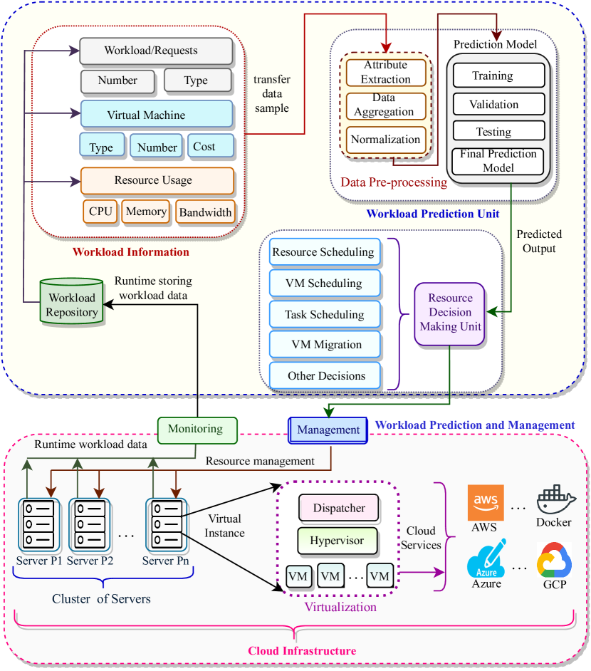
Figure 1: Schematic representation and application of Workload Prediction

The resource usage information is monitored and recorded in a workload repository within workload prediction and management unit. The raw information including number and type of requests; number, type, and cost of VMs; resource (viz., CPU, memory, bandwidth) usage, is retrieved from the repository and transferred to workload prediction unit. The significant attributes from raw data samples are extracted, aggregated, and normalized during data pre-processing. A workload prediction model is employed which generates and evolves over series of stages such as training, validation, and testing for the real-time workload prediction. The final prediction model analyzes and estimates information regarding resource usage, number and type of requests, etc. for rendering effective resource management decisions. The predicted resource information assists in assorting the needed physical resources proactively avoiding the run-time resource provisioning delay while satisfying Quality of Services (QoS) constraints.

1.3 Research Challenges

Assuredly, the cloud workload prediction plays an essential role in proactive auto-scaling and dynamic management of resources resulting into increased scalability and throughput of the systems, sustainability, fault-tolerance via proactive prediction of system failures. However, there exists some major challenges addressing the cloud workload prediction which are discussed as follows:

• Heterogeneous Workload: Cloud users submit different type of application requests, requiring heterogeneous resource capacities with varying priorities and pricing policies associated with their respective SLAs.

• Uncertain Resource Demands: The resource demand changes over time in an hour, day, week, month and years with respect to the type of workload and deadline of execution submitted by the user. Sometimes the traffic becomes bursty [24] which makes it difficult to estimate the upcoming resource demands and decide resource distribution.

• Dynamic Adaptation: Since the cloud environment is highly variable and dynamic, it suffers from unexpected fluctuations, which put forth a crucial challenge of adaptability for workload prediction i.e., to adapt or re-generate in order to sustain and perform efficiently with the changing workloads.

• Data granularity and Prediction window-size: To decide the appropriate size of data sample or granule and length of prediction window i.e., for shorter or longer interval, is another critical challenge which directly effects learning of relevant patterns and developing correlations among extracted patterns.

1.4 Paper Outline and Contributions

This paper presents a comprehensive study of machine learning based cloud workload prediction models. The study begins in Section 1 with a discussion of the CC and the vital role and research motivation for the workload prediction within CC environment. It is followed by a schematic representation with an illustrative description of the application of the load prediction and management in CDCs. Thenafter, research challenges depicting a commendable points of the need and efficacious impact of an accurate workload prediction for resource management and intervening critical issues are discussed. The operational flow outlining the essential steps of workload prediction are rendered in Section 2. The intended research methodology is discussed in Section 3. This study aims to provide an extensive review of the most prominent and seminal machine learning based models proposed for the prediction of extensive range of cloud workloads. Accordingly, Section 4 discusses Evolutionary Neural Network based prediction models, Section 5 and Section 6 entail review of Deep Learning and Hybrid learning based prediction models, respectively while Section 7 and Section 8 pertain to discuss Ensemble learning and Quantum learning based prediction models, respectively. Furthermore, the prediction models underlining the considered five categories are implemented on the common platform for evaluation and comparison of their performance in terms of various key performance indicators (KPI)s in Section 9. Finally, Section 10 concludes the study with a discussion of trade-offs among the prediction models of different classes are remarked with emerging research challenges addressing cloud workload forecasting along with their probable solution avenues are discussed. To the best of the authors’ knowledge, this is the first paper which aims to carry out a comprehensive experimental study on the machine learning based workload prediction models in the context of resource management in CC. The key contributions of this paper are:

• The commendable and recent cloud workload prediction models based on the machine-learning algorithms are designated with respect to their conceptual and operational characteristics into a classification and taxonomical organization (Fig. 3).

• To illustrate the generalized conceptual and operational design corresponding to the workload prediction approach belonging to each category, this paper figures out five specific machine learning model architectures and their working strategies.

• A critical discussion and comparison cosidering all the essential detail of state-of-the-art works are provided and their features are analyzed to determine the future research scope addressing the limitation of the respective class based prediction model.

• An implementation of the approaches associated to each of the five classes based prediction models on the same platorm is conducted for in-depth experimental analysis and comparison in terms of essential KPIs to measure their performance followed by discussion of trade-offs and notable remarks.

Table I gives the explanatory terms for the symbols, notations, abbreviations used throughout the manuscript.

TABLE I: Notations with their Explanatory Terms

Notation	Definition	Notation	Definition
$\mathcal{W}^{Ac}$	actual workload	$\mathcal{X}$	cell information
$\mathcal{W}^{Pr}$	predicted workload	$\mathcal{D}$	Input data
$\mathcal{G}_{1}$	first layer of LSTM	$\mathcal{B}$	bias
$\mathcal{CF}_{RU}$	previous resource usage information	$\mathcal{WT}$	weight matrix
$\mathcal{G}_{2}$	sigmoid layer of LSTM	${w}$	neural weight
n	number of input layer nodes	$\Theta$	qubit
p	number of nodes in hidden layer	$\mathcal{\uplus}$	activation function
z	number of base predictor (BP)	$\textit{y}^{In}$	qubit input vector
$\mathcal{MSE}$	mean squared error	$\mathcal{MAE}$	mean absolute error
m	number of data samples	ENN	evolutionary neural network
CSP	cloud service provider	CC	cloud computing
LSTM	long short term memory	CDC	cloud data centre
RNN	recursive neural network	DBN	deep belief network
Bi-LSTM	bi-directional LSTM	DNN	deep neural network
SGD	stochastic gradient descent	GRU	gated recurrent unit
PLR	piecewise linear representation	LR	logistic regression
TSA	top-sparse autoencoder	CP	canonical polyadic
OED	orthogonal experimental design	S-G Filter	savitzky-golay
PSO	particle swarm optimization	BP	back propagation
ENN	evolutionary neural network	QoS	quality of service
RMSE	root mean squared error	MAE	mean absolute error
MAPE	mean absolute percentage error	MSE	mean squared error
RMSSE	root mean segment squared error	VM	virtual machine
MRPE	mean relative predict error	DL	deep learning
CDF	cumulative distribution frequency	RMSLE	logarithmic RMSE
SaDE	Self-adaptive differential evolution	AEF	absolute error frequency
BaDE	bi-phase adaptive differential evolution	EQNN	evolutionary QNN
TaDE	Tri-adaptive differential evolution	C-NOT	controlled NOT gate
ARIMA	auto regressive integrated moving average	HL	hybrid learning
QNN	quantum neural network	EL	ensemble learning

2 Workload Prediction Operational Flow

The essential steps intended for the workload prediction are outlined via illustration of an operational design in Fig. 2. Consider input data {$\mathcal{D}_{1}$, $\mathcal{D}_{2}$, …, $\mathcal{D}_{n}$} $\in\mathcal{D}$ is extracted from the raw data stored in the workload repository.

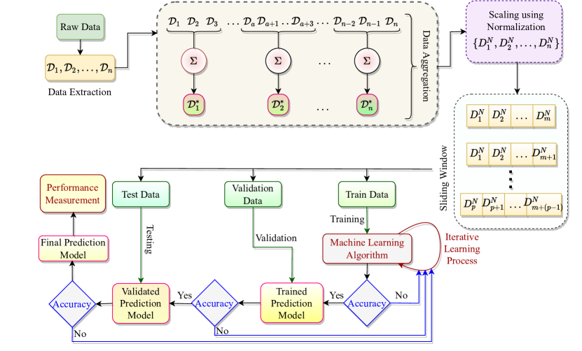
Figure 2: Load prediction operational flow

The data extraction filters relevant attributes from raw data to improve the pattern learning and developing more intuitive correlations among extracted patterns. The data aggregation operation is performed in which the extracted data is assembled as per the chosen prediction window-size (for example, five minutes) such as {$\mathcal{D}_{1}$, $\mathcal{D}_{2}$, $\mathcal{D}_{3}$} combines to produce an aggregated data sample $\mathcal{D}^{\ast}_{1}$. Similarly, {$\mathcal{D}_{a}$, $\mathcal{D}_{a+1}$, $\mathcal{D}_{a+2}$} and {$\mathcal{D}_{n-2}$, $\mathcal{D}_{n-1}$, $\mathcal{D}_{n}$} aggregate to generate data samples $\mathcal{D}^{\ast}_{a}$ and $\mathcal{D}^{\ast}_{n}$, respectively. The aggregated data samples are scaled in a specific range [$x_{a}$, $x_{b}$] and transformed into a normalized data samples {$\mathcal{D}^{N}_{1}$, $\mathcal{D}^{N}_{2}$, …, $\mathcal{D}^{N}_{n}$} using Eq. (1), where $\varpi^{In}_{min}$ and $\varpi^{In}_{max}$ are the minimum and maximum values of the input data set, respectively and the normalized data vector is denoted as $\hat{\varpi^{In}}$, which is a set of all normalized input data values. The values of $x_{a}$ and $x_{b}$ were set equals to 0.0001 and 0.999, respectively for the experiments. These normalized values are organized into two dimensional input and output matrices denoted as $\varpi^{In}$ and $\varpi^{Out}$, respectively as stated in Eq. (10):

$$\hat{\varpi^{In}}=x_{a}+\frac{d_{i}-\varpi^{In}_{min}}{\varpi^{In}_{max}-\varpi^{In}_{min}}\times(x_{b})$$ (1)

Accordingly, prediction sliding window is prepared as shown in the block of sliding window in Fig. 2. These normalized data samples are divided into three categories namely, training data, validation data, and testing data. A Machine Learning Algorithm is appointed as a prediction model which receives training data to allow specific pattern learning during iterative learning or optimization process. Thenafter, this prediction model is evaluated using any error evaluation function such as RMSE or MSE, which is tested for accuracy. If the desired accuracy is achieved, a Trained Prediction Model is obtained and validation data is passed into it again to check for prediction accuracy. If the optimal accuracy is achieved, a Validated Prediction Model is established. Finally, the test/unseen data is passed to the validated prediction model and accuracy evaluation is performed. If consecutively, the desired accuracy is achieved, a Final Prediction Model is deployed, otherwise, the respective stage of the prediction models reversed back to the iterative learning process. The performance is measured as predicted output is achieved for cloud resource management.

3 Research Methodology

This section elaborates the review methodology in detail. The review procedure includes the gathering of major cloud workload prediction papers wherein the proposed approaches are driven from machine learning algorithms and concepts. The pioneering quality prediction models, published in top-notch journals and conference databases such as IEEE, ACM Digital Library, Elsevier, Springer, Wiley are searched, studied and analysed for comparative study. Furthermore, the collected papers are refined by the identification of primary studies based on underlying proposed approaches, then application of a specific inclusion criteria for grouping the paper based on similar approaches or having overlapping features into a common class/category. To avoid any biasness during research, the review process in the remaining sections is developed by one of the authors, and finalized by the other co-author via discussions, and iterative review methods. The existing prediction models are thoroughly explored by distinct authors to ensure the completeness of the proposed study and inter-performance comparison. While selecting related work corresponding to each category, the average and below average research work are filtered and avoided so as to present a clear and concise review of the best of the existing workload prediction approaches. Accordingly, a classification and taxonomical representation is presented in Fig. 3 which designates the existing prediction models into specific classes and sub-classes of the supervised machine learning approaches based on their conceptual and operational characteristics.

Figure 3: Classification and Taxonomy of Machine learning based Workload Prediction Models

Correspondingly, the five exclusive workload prediction classes are designated as Evolutionary Learning, Deep Learning, Hybrid Learning, Ensemble Learning, and Quantum Learning. In Evolutionary learning class, the candidate approaches: ANN+SADE [25], ANN-BADE [26], ANN-BHO [27], SDWF [27], and FLGAPSONN [28] have applied evolutionary optimization alogorithms for the learning process or weight update process of neural network layers. The ample of works subject to Deep learning are further differentiated into four sub-classes including Long Short-Term Memory (LSTM) cell, Autoencoder, Deep Belief Network, and Deep Neural Network. The sub-class LSTM includes LSTM [29], 2D LSTM [30], Bi-LSTM [31], Crystal ILP [32], and FEMT-LSTM [33] which are pre-dominantly based on functionality of LSTM models. Autoencoder sub-category consists of Encoder+LSTM [34], CP Autoencoder [35], LPAW Autoencoder [36], and GRUED [37] are derived by applying some useful modification in the traditional autoencoders. Similarly, DBN+RBN [38], DBN+OED [39], DP-CUPA [40]; and es-DNN [41], DNN+MVM [42], DNN-PPE [43], SG-LSTM [44] are located with sub-class Deep Belief Network and sub-class Deep Neural Network, respectively. The Hybrid learning class represents integration of several machine learning algorithms and methods which encompasses ADRL [45], Bi-Hyprec [46], BG-LSTM [47], HPF-DNN [48], FAHP [28], ACPS [49], and LSRU [50]. Likewise, Ensemble learning involves concept of base-learners and decision making to estimate the final outcome. KSE+WMC [51], FAST [52], SGW-S [19], ClIn [53], AMS [54], E-ELM [55], and SF-Cluster [48] works enfold Ensemble learning. Finally, the Quantum learning class comprises EQNN model [56] which is developed using the principles of quantum computing and neural network learning.

4 Evolutionary Neural Network based Prediction Models

The neural networks in which the learning process is achieved with the help of an evolutionary optimization algorithm are designated as Evolutionary Neural Networks (ENN)s. Fig. 4 depicts a schematic and operational view of an ENN. Consider a feed-forward neural network $n$-$p_{1}$-$p_{2}$-$q$ comprising of $n$, $q$ nodes in input and output layers, and $p_{1}$ and $p_{2}$ nodes in three consecutive hidden layers. A training input data vector: {$\mathcal{D}_{1}$, $\mathcal{D}_{2}$, …, $\mathcal{D}_{n}$} $\in\mathcal{D}$ is passed to the input layer of this neural network, wherein each node of one layer is connected to all the nodes of the consecutive layer with the help of synaptic/neural weights {$w_{1}$, $w_{2}$, …, $w_{z}$} $\in\mathcal{W}$, $z$ is the total number of weight connections between any two consecutive neural layers. The forward propagation of training input vector ($\mathcal{D}$) is carried out via weighted connections using Eqs. (11), (12), and (13), $\uplus$ is a linear function computed at each neuron; and $\mathcal{B}$ is bias vector. The values of weight connections {$w_{1}$, $w_{2}$, …, $w_{z}$} determine impact of the input vector on the output vector of the neurons and decide strength of synaptic inter-connections between neurons.

$$\uplus=(\mathcal{D}_{1}\times w_{1})+(\mathcal{D}_{2}\times w_{2})+...+(\mathcal{D}_{n}\times w_{n})$$ (11)

$$\mathcal{D}^{\dagger}\cdot{\mathcal{W}^{\dagger}}=(\mathcal{D}_{1}\times w_{1})+(\mathcal{D}_{2}\times w_{2})+...+(\mathcal{D}_{n}\times w_{n})$$ (12)

$$\uplus=\mathcal{D}^{\dagger}\cdot{\mathcal{W}^{\dagger}}+\mathcal{B}$$ (13)

The ENN prediction model learns by adjusting the values of bias and inter-connection weights {$w_{1}$, $w_{2}$, …, $w_{n}$} $\in\mathcal{W}^{\dagger}$ of ENN with the aim of minimizing the prediction error. This learning process is achieved by applying different evolutionary optimization algorithm which selects the most optimal network from the random population of $\mathcal{Z}$ networks {$w^{\dagger}_{1}$, $w^{\dagger}_{2}$, …, $w^{\dagger}_{\mathcal{Z}}$}. The algorithm repeatedly optimizes the values of neural weight connections by updating the population of networks exploring and exploiting the diverse population of networks extensively. During successive epoch, the best network candidate is chosen by evaluating a fitness function such as prediction error estimation using Root Mean Squared Error (RMSE), Mean Absolute Percentage Error (MAPE) etc. To allow the online optimization of ENNs, the learning process is periodically repeated with the previous and most recent samples of workloads for their training and re-training in an off-line mode while analysing the live workloads concurrently in the real-time. There are several approaches proposed using ENN for cloud workload prediction and this section further aimed at providing comprehensive discussion and analysis of these approaches.

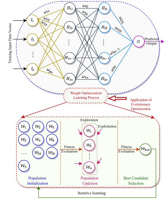
Figure 4: ENN based load prediction

An ENN-based cloud workload prediction approach is proposed in [25] wherein a three layered feed-forward neural network is trained using a Self adaptive Differential Evolution (SaDE). During the learning process, the population of networks is updated by applying exploration and exploitation operations using three mutation strategies selectively followed by uniform crossover. This approach produced improved accuracy over Backpropagation trained neural network (BPNN) [57] because of multidimensional learning in former as compared with optimizing single solution in later approach. Kumar et al. [26] have proposed a Biphase adaptive Differential Evolution (BaDE) learning based neural network that adopted a dual adaptation viz., at level of crossover during exploitation process and mutation in exploration phase to improve the learning efficiency of neural network. As a consequence, this work outperformed SaDE [25] in terms of prediction accuracy. An auto-adaptive neural network is developed in [58] wherein the network connection weights are adjusted with Tri-adaptive Differential Evolution (TaDE) algorithm. In this approach, the adaptation is appointed at level of crossover, mutation, and control parameters generation level which allows enhanced learning the prediction model. Kumar et al. [59] have used a BlackHole Optimization (BHO) algorithm to optimize neural weights and develop a workload prediction model for dynamic resource scaling. This evolutionary optimization algorithm updates the movement of the stars i.e., randomly intialized network vectors and track their position whether reaching an event horizon. Further, this work was enhanced by modifying the existing BHO algorithm as enhanced BHO (i.e., E-BHO) in [27] by including concepts of local and global blackhole (i.e., best solution) during iterative learning process of the feed-forward neural network. Also, this approach has computed the deviation in recent forecasts and applied it to enhance the accuracy of the forthcoming predictions. Malik et al. [28] have proposed an ENN based multi-resource utilization prediction approach. In this work, Functional Link Neural Network (FLNN) with a hybrid evolutionary algorithm comprising of Genetic Algorigm (GA) and Particle Swarm Optimization (PSO) is applied for neural network weight adjustment during learning process. It has been compared with FLNN, FLNN with GA (FLGANN), and FLNN with PSO (FLPSONN) and validated its performance against these methods.

A pandect summary of existing ENN-based workload prediction models are provided in Table II which highlights the major features, implementation details, performance metrics, parameter tunings and intended computational complexities during the learning process. The approaches discussed in [25, 26, 58] are based on Differential Evolution which needs tuning of multiple control parameters including crossover-rate, mutation-rate, keeping track of dynamic or fixed learning-period, maintaining records of the number of failure and successful candidates during each epoch. While the prediction approaches entailed in [59, 27] employing BHO keeps track of event-horizon radius only and updates the next generation population depending on the comparison of the fitness value of each candidate with the horizon radius. Hence, it can be analysed that the consumption of training time and involved computational complexity, number of training epochs are higher for DE based prediction approaches as compared with that of BHO based prediction. Based on the aforementioned factors, [27] is the most admissible among all the discussed approaches.

TABLE II: Summary and Comparison of ENN-based Prediction Approaches

Notable Contributors (Timeline)	Model/ Approach/ Framework	Workflow/ Strategy	Datasets	Implementation/ Simulation tool	Predicted parameters	Error metrics	Results or Remarks
Kumar et al. [25] (2018)	ANN-SaDE	Feed-forward neural network is trained with self-adaptive differential evolutionary algorithm	NASA and Saskatchewan	MATLAB	Number of requests per unit time	MSE	reduced error up to 0.001 and accuracy improved by 168 times over BP
Kumar et al. [26] (2020)	ANN-BaDE	three mutations stategies and three crossover strategies based adaptation within DE algorithm optimizes ANN	NASA, Saskatchewan, Google Cluster traces	Python	Number of requests, CPU, memory usage	MSE	accuracy improved up to up to 91% and 97% over SaDE and BP, respectively
Saxena et al. [58] (2020)	ANN-TaDE	three mutations stategies and three crossover strategies with control parameter-tuning based adaptations within DE algorithm optimizes ANN	NASA and Saskatchewan	Python	Number of requests per unit time	RMSE	accuracy improved by 97.4% and 94.8% over BP and SaDE, respectively
Kumar et al. [59] (2016)	Neural Network with BlackHole Optimization	Blackhole algorithm is utilized in the learning process of neural network provoded with pre-processed training data	HTTP traces from NASA, Calgary and Saskatchewan web servers	MATLAB	Number of requests per unit time	MSE	error reduced upto 134 times over BP
Kumar et al. [27] (2021)	Self directed workload forecasting method (SDWF)	the forecasting error trend is captured by computing the deviation in recent forecasts and applied to enhance the accuracy of further predictions	NASA and Saskatchewan HTTP traces, Google Cluster	MATLAB	Number of requests, CPU, memory usage	MSE	error up to 99.99% over compared methods
Malik et al. [28] (2022)	FLGAPSONN: FLNN +GA+ PSO	Pre-processed training data is passed to FLNN which is optimized with hybrid algorithm of GA and PSO	Google Cluster traces	Python	CPU, memory, disk usage	MAE	improved accuracy by 21.87%, 13.75%, and 30.55% over FLPSONN, FLGANN, and FLNN, respectively

5 Deep Learning based Prediction Models

Deep Learning models are a class of prediction models which have immensely influenced the field of cloud computing. A conceptual and operational design of deep learning strategy is illustrated in Fig. 5, wherein, the pre-processed training input data samples: {$\mathcal{D}_{1}$, $\mathcal{D}_{2}$, …, $\mathcal{D}_{n}$} are passed into a deep learning algorithms such as Long Short-Term Memory (LSTM), Gated Recurrent Units (GRU), Deep Belief Networks (DBN), Deep Feed-forward Neural Network (DNN), Autoencoders, Recursive Neural Network (RNN) and so on for the learning process. The essential hyperparameters {$Hyp1$, $Hyp2$, …, $HypN$} of the respective deep learning algorithms are tuned and re-tuned periodically to create and update the deep learning based prediction model. The trained model is further evaluated using validation data to estimate its performance and accuracy. Accordingly, a deep learning based model optimized with best or most admissible hyperparameters is obtained.

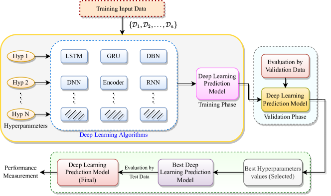
Figure 5: Deep Learning based Prediction Operative View

For instance, LSTM based deep learning algorithm is applied for the prediction. The resource usage of actual load ($\mathcal{Z}^{Ac}_{\mathcal{RU}}$) stored as a historical workload is fed as input into neural network input layer for prediction of future resource usage. LSTM-RNN based prediction model comprises of cells containing four neural network layers, where previous cell ($\mathcal{X}^{t-1}$) information is passed to current cell ($\mathcal{X}^{t}$). The first layer ($\mathcal{G}_{1}$) applies Eq. (14) to decide the amount of previous resource usage information ($\mathcal{CF}_{\mathcal{RU}_{i}}^{t}$) which is tranferred to the next state; where $\mathcal{WT}$ is weight matrix, $\mathcal{B}$ is a bias value, $\mathcal{Z}^{Pr}_{t-1}$ and $\mathcal{Z}^{Pr}_{t}$ are previous output and current input, respectively. The cell state is updated using two network layers viz., $sigmoid$ layer ($\mathcal{G}_{2}$) which decides the values to be updated ($\mathcal{I}^{t}$) using Eq. (15), and $tanh$ layer for generation of a new candidate values vector ($\hat{\mathcal{X}}^{t}$) using Eq. (16). Finally, Eq. (17) combines both outputs to update cell state.

$$\mathcal{CF}_{\mathcal{RU}_{i}}^{t}=\mathcal{G}_{1}(\mathcal{WT}_{\mathcal{CF}}\cdotp[\mathcal{Z}^{Pr}_{t-1},\mathcal{Z}^{Ac}_{t}]+\mathcal{B}_{\mathcal{RU}})$$ (14)

$$\mathcal{I}^{t}=\mathcal{G}_{2}(\mathcal{WT}_{\mathcal{I}}\cdot[\mathcal{Z}^{Pr}_{t-1},\mathcal{Z}^{Ac}_{t}]+\mathcal{B}_{\mathcal{I}})$$ (15)

$$\hat{\mathcal{X}}^{t}={tanh}(\mathcal{WT}_{\mathcal{X}}\cdot[\mathcal{Z}^{Pr}_{t-1},\mathcal{Z}^{Ac}_{t}]+\mathcal{B}_{\mathcal{X}})$$ (16)

$$\mathcal{X}^{t}=\mathcal{CF}_{\mathcal{RU}_{i}}^{t}\times\mathcal{X}^{t}+\hat{\mathcal{X}}^{t-1}\times\mathcal{I}^{t}$$ (17)

The RU of predicted traffic ($\mathcal{Z}^{Pr}_{t+1}$) for different VMs hosted on a server are aggregated to determine any overload proactively and alleviate it by migrating VMs with highest predicted RU to an efficient server. A comprehensive survey of the existing workload prediction models belonging to four distinct categories of deep learning approaches are discussed in the subsequent sections.

5.1 LSTM-RNN

A fine-grained cloud workload prediction model using long short-term memory based recurrent neural network (LSTM-RNN) is presented in [29] which is capable of learning a long-term dependencies and producing a high accuracy for host load prediction. Tang [30] has proposed a two-dimensional LSTM neural network cell structure by utilizing a hidden layer week-based dependence and weights parallelization algorithm. This work has improved LSTM algorithm by providing the mathematical description of parallel LSTM algorithm and its optimization with an error back propagation method. Its performance is validated using the real workload of the Shanghai Supercomputer Center. Tuli et al. [34] have proposed an automatic straggler (slow processing tasks) prediction and mitigation method for cloud environment using an encoder LSTM network that addressed heterogeneous host and volatile task characteristics. The encoder analyses the resource usage and load information and passes the information to the LSTM. Further, an exponential moving average of input matrices is taken into account to prevent the LSTM model from diverging. A storage workload prediction approach named CrystalLP based on LSTM neural network is introduced in [32]. In this approach, a storage workload time-series model is developed which collects the intended workload patterns that helps in precise and adaptive scheduling with load balancing. Thereafter, LSTM based workload predictor is implemented which is trained or optimized with an algorithm composed of an integration of stochastic gradient descent (SGD) together with the Adam optimizer. Gao et al. [31] have presented a multi-layer Bi-directional Long Short Term Memory (Bi-LSTM) based task failure prediction algorithm. It comprises of one input layer, two Bi-LSTM layers, one output layer and the Logistic Regression (LR) layer to predict whether the tasks are failed or finished. Unlike traditional LSTM which uses only forward state, Bi-LSTM operates on both forward and backward states to allow more accurate estimation of the weights of both closer and farther input features. Ruan et al. [33] have established a turning point prediction model for cloud server workload forecasting considering cloud workload features. Thenafter, a cloud feature-enhanced deep learning model with rule-filtering based Piecewise Linear Representation (PLR) algorithm is build for workload turning point prediction. The performance evaluation of this model illustrated its prediction accuracy effectiveness in terms of improvement in F1 score over existing state-of-the-art methods.

5.2 Auto-encoder

An efficient canonical polyadic (CP) decomposition based deep learning model is proposed in [35] for prediction of industrial workloads in cloud, wherein, a CP auto-encoder is constructed by converting a basic autoencoder into tensor space with the help of bijection. In this model, the basic auto-encoder in the CP decomposition format is followed by the stacked autoencoder model in the CP decomposition format. The stacked autoencoder is created to learn the relevant features of the workload information and the CP decomposition is employed to compress the features substantially for improving the training efficiency. Chen et al. [36] have established a deep Learning based Prediction Algorithm for cloud Workloads (L-PAW) which included a Top-Sparse Auto-encoder (TSA) for an effective extraction of the essential representations of workloads. This approach integrated GRU and recurrent neural network (RNN) to evict the long-term memory dependencies for prediction of forthcoming cloud workloads with enhanced accuracy.

5.3 Deep Belief Network

Qiu et al. [38] have proposed a Deep Belief Network (DBN) composed of multiple-layered Restricted Boltzmann Machines (RBMs) and a regression layer for prediction of cloud workloads. In this model, DBN extracts the high level features from all VMs and the regression layer is used to predict the forthcoming load on VMs. It learns significant patterns efficiently using prior knowledge in an unsupervised manner. Zhang et al. [39] developed a DBN approach based load prediction model which is a stacked RBM and used Backpropagation algorithm to minimize its loss function. It incorporated analysis of variance and Orthogonal Experimental Design (OED) techniques into the parameter learning of DBN and have achieved a high prediction accuracy over ARIMA. Also, a similar DBN-based approach is presented in [60] which can capture high variances in cloud metric data without handcrafting specified feature for short term resource demands and long-term load prediction. Wen et al. [40] have presented a DBN and Particle Swarm Optimization (PSO) based CPU usage prediction algorithm named as DP-CUPA. This algorithm includes three main steps: pre-processing of training data samples; adoption of autoregressive and grey models as base prediction models; and training of DBN. The PSO is utilized for estimation of DBN parameters during learning process.

5.4 Deep Neural Network

Xu et al. have proposed an efficient supervised learning-based Deep Neural Network (esDNN) algorithm [41] to extract and learn the features of historical data and accurately predict future workloads. The multivariate data is converted into supervised learning time series and a revised GRU is applied which can adapt to the variances of workloads to achieve accurate prediction and overcome the limitations of gradient disappearance and explosion. A DNN based workload prediction method (designated as DNN-MVM) is developed in [42] to handle the workload prediction from multiple virtual machines. It employed a pre-processing and feature selection engine to handle data directly from these virtual machines. The model classifies data based on historical loads to provide enhanced information or knowledge to the cloud service provider for resource management and optimization. It is useful to predict the peak demands of resources in the future. This model is validated using Grid Workload Archive (GWA) dataset. Bi et al. [44] have proposed another DNN based workload prediction model wherein a logarithmic operation is performed ahead of task smoothening to minimize the standard deviation. Thenafter, a Savitzky-Golay (S-G) filter is applied to eliminate the extreme points and noise interference in the sequence of the original data. The DNN based LSTM (SG-LSTM) is employed to extract complicated characteristics of a task time series. A Back Propagation Through Time (BPTT) algorithm is implemented by adopting gradient clipping method to eliminate a gradient exploding problem and optimization of the model is accomplished using Adam Optimizer. The model is evaluated with Google Cluster dataset to confirm its efficacy over existing methods. A DNN learning based Power Prediction Engine (DNN-PPE) is proposed in [43] which includes data acquisition, data pre-treatment, and prediction modules. Recursive auto encoder is utilized for short-time fine-grained prediction that can track the rapid changes of the power consumption within a data centre.

TABLE III: Comparative Summary of Deep Learning-based Prediction Approaches

Notable Contributors (Timeline)	Model/ Approach/ Framework	Workflow/ Strategy	Datasets	Implementation/ Simulation tool	Predicted parameters	Error metrics	Results or Remarks
Kumar et al. [29] (2018)	LSTM-RNN	Combinations of networks in loop retains learning information, performs specific operation to produce output for next network in loop	Web server HTTP traces	MATLAB	No. of requests per unit time	MSE	reduced RMSE up to 0.00317
Tang [30] (2019)	2-D LSTM	Input data is analysed on week dependence basis and weights parallelization algorithm is used for improved optimization of LSTM	l workload of the Shanghai Supercomputer	Not mentioned	Workload over days	MSE	accuracy improved for large-scale real-time cloud services
Tuli et al. [34] (2021)	Encoder LSTM	Encoder is used for input matrices preparation and LSTM predicts the load information	PlanetLab traces	CloudSim and Python	CPU, Memory, Bandwidth	MSE, MAPE	reduced execution time, resource contention, energy and SLA violations by 13%, 11%, 16% and 19%
Gao et al. [31] (2020)	Bi-LSTM	Training data propagates via input layer, two Bi-LSTM layers, one output layer and LR layer during learning process	55,55,55 tasks traces	Tensorflow in Python	task failure rate	F1-Score	93% accuracy and 87% task failure correctly predicted
Ruan et al. [32] (2021)	CrystalLP	Time-series model collects load patterns and LSTM trained with SGD+Adam optimizer predicts load	Web search archive SPC traces	Keras library, Python	Request size	MAPE, RMSE, MAE	achieved 1.10% improvement in MAPE, and better performance in MAE over existing methods
Ruan et al. [33] (2022)	FEMT-LSTM	a turning point prediction model considering cloud workload features followed by feature-enhanced deep learning model is developed	Google Cluster, Alibaba, HPC Grid workloads	Keras library, Python	CPU usage	binary cross-entropy, F1, precision, recall	F1 score is improved by 6.6% over existing approaches
Zhang et al. [35] (2018)	CP auto-encoder	canonical polyadic decomposition compresses the features and stacked auto-encoder learns the patterns for prediction	PlanetLab traces	MATLAB	CPU utilization	MAPE, RMSE	achieves a higher training efficiency and prediction accuracy for industrial workloads
Chen et al. [36] (2019)	L-PAW auto-encoder	TSA extracts workload patterns and GRU+RNN prdicts the upcoming load	TensorFlow 1.4.0, Python	DUX-cluster, Alibaba, and Google cluster	CPU, memory, disk I/O usage	MSE, CDF	outperformed the accuracy of LSTM, RNN, GRU
Qiu et al. [38] (2016)	DBN+RBMs	DBN extracts significant patterns while learning and regression is used for prediction	PlanetLab traces	CloudSim	CPU utilization	MAPE	improved the performance up to 1.3% over existing method
Zhang et al. [39] (2017)	DBN+OED	Pre-processed data is passed into DBN+OED model which is tuned with Backpropagation algorithm	Google Cluster traces	Python	CPU, RAM usage	MSE	MSE achieved in the range [$10^{-4}$, $10^{-3}$]
Wen et al. [40] (2020)	DP-CUPA	DBN predicts the load information and PSO estimates the fitness values of its tuning parameters	Google Cluster traces	not mentioned	CPU usage	MSE, MAPE, MAE	outperformed autoregressive, DBN, Grey model
Xu et al. [41] (2022)	es-DNN	supervised learning converts multi-variate data into time-series and modified GRU is applied	Alibaba and Google Cluster traces	TensorFlow 2.2.0 in Python	CPU usage per time-unit interval	MAPE, MSE, RMSE	reduced number of active hosts efficiently and optimized cost
Bhagtya et al. [42] (2021)	DNN-MVM	Selected data from multiple VMs is classified, preprocessed and passed to DNN-MVM for learning process	Grid Workload Archive (GWA) traces	Google Colab using Keras	CPU, Memory, and Disk Utilization	MSE	achieved more than 85% prediction accuracy for each resource
Bi et al. [44] (2019)	SG-LSTM	S-G filter provides smoothen data to LSTM for more accurate prediction	Google traces	Python	CPU, Memory	Logarithmic RMSE, $R^{2}$	outperformed BPNN, LSTM, SG-LSTM, and SG-BPNN
Li et al. [43] (2016)	DNN-PPE	Preprocessed data is passed to Recursive Auto Encoder	world cup 98 (WC98) and Clark net traces	Python	Power, No. of requests	-	79% error reduction over canonical prediction

6 Hybrid Prediction Models

The prediction models based on hybrid machine learning combines different machine learning algorithms (say $N$ algorithms) and feed the outcome of one algorithm to another (one-way) to create an efficient machine learning model for precise and accurate predictions. These hybrid models are build using various collaborations such as ‘Classification + Classification’; ‘Classification + Clustering’; ‘Clustering + Clustering’; ‘Clustering + Classification’; ‘Classification + Regression’; ‘Clustering + Regression’ etc. These combinations are selected as per the requirement and challenges respective to the intended problem to minimize features noise and biasness, reduce variance, and enhance the accuracy of prediction. A schematic representation of hybrid prediction model is depicted in Fig. 6.

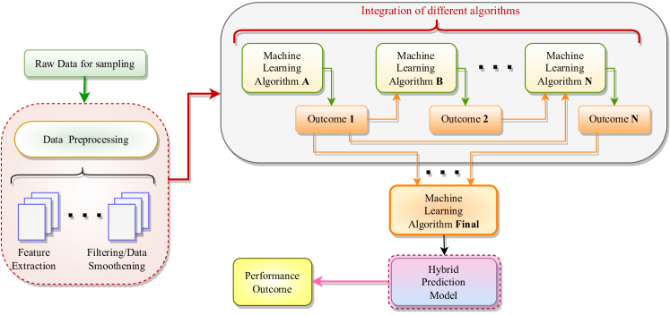
Figure 6: Hybrid Prediction Model

In this model, the raw and complex data samples are pre-processed by filtering and smoothening the data samples via extraction of significant features, aggregation, and scaling or normalization. The pre-processed data samples passes through a series of $N$ machine learning algorithms feeding their outomes as an input to other machine learning algorithm, generating a hybrid prediction model for performance measurement and deployment for the intended purposes. The significant key contributions related to hybrid approach based workload prediction models are discussed below.

Kardani et al. [45] have developed a hybrid Anomaly-aware Deep Reinforcement Learning-based Resource Scaling (ADRL) for dynamic resource scaling in the cloud environment. It presents an anomaly detection method for Deep Reinforcement Q-Learning-based decision making scheme that identifies anomalous states in the system and triggers actions accordingly. This work includes two levels of global and local decision-makers to govern the necessary scaling actions. ADRL improved the QoS with essential actions only and increased stability of the system. A hybrid Recurrent Neural Network (RNN) based prediction model named ‘BHyPreC’ is proposed in [46] which comprises of Bidirectional Long Short-Term Memory (Bi-LSTM) on top of the stacked LSTM and GRU for prediction of VM resource usage. It improves the non-linear data analysis capability of Bi-LSTM, LSTM, and GRU models separately and confirmed better accuracy compared with other statistical models. It uses combined grid search technique of historical window size to optimize the model and determine the best possible set of window size. Bi et al. [47] proposed integrated deep learning method named ‘BG-LSTM’ which incorporates BiLSTM and GridLSTM to achieve high-quality prediction of workload and resource time series. During preprocessing, it applies a filter of Savitzky-Golay (SG) to reduce the standard deviation before smoothing workload. It can effectively extract complex and non-linear features of relatively longer time series and achieve high prediction accuracy. A Hierarchical Pythagorean Fuzzy Deep Neural Network (HPFDNN) is proposed in [61] to predict the amount of cloud resources requirement. The neural representations of original sampling data are used as a supplementary approach for clear interpretations of true results which is beyond the use of fuzzy logic. The users can determine the expected quantity of cloud services utilizing the forecasts of the deep neural network which will help in reducing cost.

A hybrid autonomous resource provisioning model based on MAPE-k control loop for multi-tier applications is presented in [28]. It is a combination of the Fuzzy Analytical Hierarchy Process approach named as ‘ FAHP’. The experimental results indicate that the proposed solution outperforms in terms of allocated virtual machines, response time, and cost compared with the other approaches. An Adaptive Classified Prediction Scheme (ACPS) is proposed in [49] which first categorises the workloads into different classes that are automatically assigned for different prediction models according to workload features. Further, the problem of the workload classification is transformed into a task assignment by establishing a mixed 0–1 integer programming model which is solved quickly by utilizing an improved branch and bound algorithm. Peng et al. [37] have applied a GRU based Encoder-Decoder network named ‘GRUED’ containing two Gated Recurrent Neural Networks (GRNNs) to address these issues. It has been evaluated via experiments for the prediction of multi-step-ahead host workload in cloud computing. Shuvo et al. [50] have proposed a novel hybrid-method named ‘LSRU’ for improving the prediction accuracy. LSRU is an integration of LSTM and GRU for short-time ahead prediction along with long-time ahead prediction with sudden burst of workload.

TABLE IV: Comparative Summary of Hybrid Machine Learning-based Prediction Models

Notable Contributors (Timeline)	Model/ Approach/ Framework	Workflow/ Strategy	Datasets	Implementation/ Simulation tool	Predicted parameters	Error metrics	Results or Remarks
Kardani et al. [45] (2021)	ADRL: Deep RL+Q-Learning	Deep Q-learning based RL model to respond CPU and memory bottleneck problem that help in resource scaling and decision making	Web-based Rice University Bidding System (RUBiS)	Python with Java-based CloudSim	CPU, Memory, Response-time	MSE	improved QoS and stability
Karim et al. [46] (2021)	BiHyPrec: Bi-LSTM + LSTM + GRU	Pre-processed data is given to collaborative model of Bi-LSTM, LSTM, and GRU units that accomplishes a deep learning-based approach to effectively tackle the complexity and non-linearity of time series data	Bitbrains traces	Python and Google Colaboratory	CPU usage	MSE, MAPE, MAE, RMSE	performs better over ARIMA, LSTM, GRU, Bi-LSTM
Bi et al. [47] (2021)	BG-LSTM: Bi-LSTM + GridLSTM	Savitzky-Golay (SG)is used to smoothen data which is passed to hybrid model of Bi-LSTM and GridLSTM for prediction	Python	Google Cluster traces	CPU and RAM usage	MSE, RMSLE, $R^{2}$	better accuracy over SG-LSTM, SG-Bi-LSTM, SG-GridLSTM
Chen et al. [61] (2021)	HPFDNN: Hierarchical Pythagoras + Fuzzy DNN	Pythagorean fuzzy logic, neural representations, and deep neural network are integrated and network training method with adaptive learning rate is adopted to minimize the cost of cloud services for users	Carnegie Mellon University dataset	Not mentioned	Number of requests	Accuracy cost and total cost	saved 202.48 dollars for real-time requests over existing methods
Khorsand et al. [28] (2018)	FAHP	FAHP and SVR algorithms are developed for workload prediction and resource provisioning and the appropriate autoscaling decisions	Clark Net, NASA, Synthetic workload	CloudSim and Open source RUBIS	Request arrival, response time, cost	MSE, NMSE, RMSE, RMSSE	Reduces cost of rental resources for cloud service provider with QoS
Liu et al. [49] (2017)	ACPS	Distinct prediction models are automati- cally assigned depending on the workload features	Google Cluster traces	Python	Response time and Cost	Mean error, mean relative prediction error (MRPE)	Prediction error is reduced by 40.86% over Linear Regression
Peng et al. [37] (2018)	GRUED	GRU encoder maps a variable-length workload sequence to a fixed-length vector, and the GRU decoder maps the vector representation back to a variable-length future workload series	Google Cluster and Dinda workloads	Python, UNIX system	CPU, Job arrivals	MAE, MAPE, RMSE, root mean segment squared error (RMSSE)	Reduce prediction error over LSTM
Shuvo et al. [50] (2020)	LSRU: LSTM + GRU	Some statistical methods such as AR, ES, ARMA, and ARIMA for forecasting and passed to LSTM and GRU combined unit for an improved prediction accuracy	Bitbrains	Kaggle	CPU, Disk, memory, bandwidth	MAE, MAPE, RMSE, MSE	Reduce prediction error over LSTM and GRU

7 Ensemble Prediction Models

An ensemble approach involves the use of multiple ‘Base Prediction’ ($BP$) models or ‘Experts’ to forecast the expected future outcome of an event. The final outcome of an ensemble model is computed by combining the forecasts of each expert using a voting engine. The conceptual architecture of an ensemble based predictive approach is illustrated in Fig. 7.

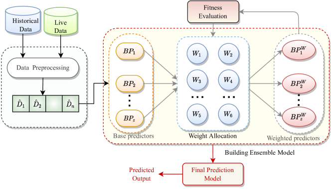
Figure 7: Ensemble Prediction Model

The historical and live data samples are pre-processed and a ‘sliding window’ is prepared and the input data vector thus created is given as input to all the base predictors {$BP_{1}$, $BP_{2}$, …, $BP_{z}$}, where $z$ is the number of base predictors used for ensemble learning. The estimated outcome of each base predictor is assigned a weight value indicating their significance in the final prediction outcome. The weight allocation and their updation requires a learning process using suitable optimization method such as multi-class regression, priority based method, or evolutionary learning algorithm. The ensemble learning approach is more effective over the individual prediction method that suffers from challenges like, high variance, low accuracy, feature noise and bias. Basically, in ensemble approach, the various machine learning models work independently of each other to give a prediction and a voting system (hard or soft voting) based on weighted values associated to each base predictor determines the final prediction. The prominent models based on ensemble learning are discussed below.

Singh et al. [51] have addressed the problem of extensive range of workloads prediction by extending and adapting two online ensemble learning methods including Weighted Majority (WM) and Simulatable Experts (SE). The classical SEs are extended from binary outcome space to k-outcome space to make them suitable for solving any k-class problem (designated as ‘kSE’). The Weighted Majority ensemble model parameters are regenerated incrementally making these algorithms computationally more efficient and suitable for handling massive range of online data streams (designated as ‘WMC’). These models are evaluated using large datasets of 1570 servers and have verified that approximately 91% servers can be correctly predicted with the extended versions of these algorithms. Feng et al. [52] have proposed an ensemble model for Forecasting workloads with Adaptive Sliding window and Time locality integration named FAST. An adaptive sliding window algorithm is developed considering correlations of trend and time, and random fluctuations of forthcoming workloads to maximize accuracy of prediction with lower overhead. Also, a time locality concept for local-predictor behavior is accomplished for the error-based integration strategy. The entire model is integrated by developing a multi-class regression weighting algorithm. The performance of the model is validated using Google Cluster trace datasets. An integrated model for temporal prediction of workloads is proposed in [19] which combines Savitzky–Golay (SG) filter and wavelet decomposition with stochastic configuration networks to predict approaching workload. In this model, a task time series is smoothened using SG filter and decomposed into components via wavelet decomposition method. This model named ‘SGW-S’ is able to characterize the statistical features of both trend and detailed components and achieved an improved performance with faster learning.

A cloud resource forecasting model named ‘CloudInsight’ (ClIn) based on ensemble prediction approach is proposed in [53]. This model meticulously locates the most admissible machine learning prediction approach by training a statistical features based classifier for the accurate estimation of job arrivals. It employs a number of local predictors or experts and builds an ensemble prediction model using them by dynamically determining the significant weights (or contributions) of each local predictor. The adaptive weight scores are optimized at regular intervals with the help of multi-class regression with a SVM classifier for selection of the most appropriate prediction model with highest accuracy during respective prediction interval. This model is tested using three different categories of workloads including: web, cluster and high performance computing workloads to prove its efficacy over existing prediction models. Baig et al. [54] have proposed an ensemble and adaptive cloud resource estimation model named ’Adaptive Model Selector’ (AMS). This model determines the most admissible machine learning prediction approach by training a statistical features based classifier for the accurate estimation of resources utilization. It builds a classifier using Random Decision Forest (RDF) to predict the best model for a given sliding window data by training and re-training periodically at regular time-intervals. The selected features and identified prediction methods are logged as training data and passed to sliding window for learning process. The performance of this model is evaluated using Google Cluster, Alibaba, and Bitbrains datasets. Kumar et al. [55] have presented an ensemble learning based workload forecasting model named ‘E-ELM’ that uses extreme learning machines and their associated forecasts are weighted by a voting engine. In this work, a metaheuristic algorithm inspired by blackhole theory is applied to decide the optimal weights. The accuracy of the model is evaluated for CPU and memory demand requests of Google cluster traces and for CPU utilization of PlanetLab VM traces. Chen et al. [48] have proposed a self-adaptive prediction method using ensemble model and subtractive-fuzzy clustering based fuzzy neural network (ESFCFNN). The user preferences and demands are characterized and an ensemble prediction model is constructed using several base predictors.

TABLE V: Comparative Summary of Ensemble Learning-based Prediction Approaches

Notable Contributors (Timeline)	Model/ Approach/ Framework	Workflow/ Strategy	Datasets	Implementation/ Simulation tool	Predicted parameters	Error metrics	Results or Remarks
Singh et al. [51] (2014)	kSE+WMC	SE is extended to k-outcome space and WM is improved for incremental and computationally efficient learning process	Dataset G(1570)	Not mentioned	server workload	MAPE	89% accurate predictions as compared with 13–24% for baseline algorithms
Feng et al. [52] (2022)	FAST	The adaptive sliding window considers all types of workload trends with time locality concept for error-based integration is developed to enhance prediction accuracy	Google Cluster traces	Python	CPU, memory	Absolute Error, RMSE, $R^{2}$	improved prediction accuracy by 14.99% to 27.55on RMSE and 22.57% to 76.86% on $R^{2}$
Bi et al. [19] (2019)	SGW-S	SG filter and wavelet decomposition is integrated with stochastic configuration networks to predict workload with high accuracy	Google Cluster traces	Not mentioned	task arrival rate	MSE, $R^{2}$	Use of SG-filter with wavelet decomposition helps improve the prediction accuracy
Kim et al. [53] (2020)	ClIn: ensemble with multi-class regression	Different local predictors constitutes an ensemble prediction model by dynamically determining and updating the significant weights of each predictor	Web, cluster, HPC Grid workloads	Python	Job arrival per unit time	Normalised RMSE, Absolute Error	Up to 15%–20% less under-/over-provisioning with high cost-efficiency and low SLA violations
Baig et al. [54] (2019)	AMS	Predict the forthcoming resource demand with the best predictor model as selected by the RDF classifier which is updated periodically with time	Alibaba, Bitbrains, Google Cluster	Python	CPU	RMSE, MAE	improved prediction accuracy from 6%-27% over current methodologies
Kumar et al. [55] (2020)	E-ELM	ELM based local predictors are trained and selected by employing a weight updation method with a help of a metaheuristic algorithm	MATLAB	Google Cluster and PlanetLab traces	CPU, memory	RMSE, MAE	RMSE reduced up to 99.20% over existing methods
Chen et al. [48] (2015)	Subtractive-fuzzy clustering	user preferences and demands are characterized into an ensemble prediction model subtractive-fuzzy clustering based fuzzy neural network	Data Flow Statistics traces	CloudSim	Network resource traces	MSE, MAE	Effective in resource demand prediction

8 Quantum Neural Network based Prediction Models

A Quantum Neural Network (QNN) based prediction model is an intelligent model for prediction with the machine learning capabilities of neural network and computational proficiency of quantum mechanics to achieve prediction accuracy with high precision. Basically, it is a neural network comprising of Qubit neurons and Qubit weights instead of real-numbered values and the training data information is also propagated in the form of Qubits. A Qubit is represented as a one, a zero, or any quantum superposition of these states. Mathematically, it can be realized as: $|\Psi\textgreater=\alpha|0\textgreater+\beta|1\textgreater$, where $\alpha$ and $\beta$ are complex numbers specifying the probability amplitudes of states $|0\textgreater$ and $|1\textgreater$ respectively. The schematic representation of QNN based prediction model is shown in Fig 8 which comprises of one input, multiple hidden and one output layers having $n$, $p$ and $q$ qubit nodes, respectively which represents $n$-$p$-$q$ Qubit network architecture. The inter-connection weights between Qubit neurons of different layers are also taken in the form of Qubits that are adjusted during learning process.

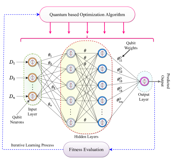
Figure 8: Quantum Neural Network

The state transitions of Qubit neurons are derived from the various Quantum gates such as Rotation gate, Controlled-Not gate etc. The training data samples values are extracted and aggregated into a specific time-interval such as 5 minutes which are scaled in a specific range using a normalization function. The normalized data values are transformed into quantum state values or Qubits by applying the effect of qubit rotation using Eqs. (18) and (19);

$${y^{In}}_{i}=f({\Theta_{i}}^{In})$$ (18)

$$\Theta_{i}=\frac{\pi}{2}\times\mathcal{D}_{i}$$ (19)

where $\mathcal{D}_{i}$ is the $i^{th}$ input data point, $\Theta_{i}$ is $i^{th}$ Quantum input point to the network. The QNN model extracts relevant and significant patterns from actual workload and analyzes $n$ previous workload values to estimate forthcoming workload information at the next $(n+1)^{th}$ instance of time within the datacentre. The learning process of QNN is derived by a Qubit based optimization algorithm that can manipulate, explore, and exploit Qubits to regenerate the population and prevent the problem of stagnation. The workload prediction methods using QNN is still at an infancy stage.

The only work established thus far using QNN based model for workload prediction is proposed in [56]. This model exploits the computational efficiency of quantum computing by encoding workload information into Qubits and propagating this information via network for estimatimation of the workload or resource demands with enhanced accuracy proactively. The rotation and reverse rotation effects of the C-NOT gate served the activation function at the hidden and output layers to optimize the Qubit weights. Self Balanced Adaptive Differential Evolution (SB-ADE) algorithm is developed to optimize qubit network weights. This model is evaluated using three different categories of workloads where the prediction accuracy is substantially is improved over the existing approaches. A workload prediction model using complex numbers, is presented in [62] where a high capability of learning and better accuracy is applied to multi-layered neural networks with multi-valued neurons (MLMVN) prediction model in less time.

9 Performance Evaluation

9.1 Experimental Set-up

The simulation experiments are conducted on a server machine assembled with two Intel^® Xeon^® Silver 4114 CPU with a 40 core processor and 2.20 GHz clock speed. The computation machine is deployed with 64-bit Ubuntu 16.04 LTS, having 128 GB RAM. All the selected best prediction works based on Evolutionary Neural Network (ENN), Ensemble Learning (EL), Hybrid Learning (HL), Deep Learning (DL), Evolutionary Quantum Learning were implemented in Python 3.7 with the details of various intended parameters with their values listed in Table VI.

TABLE VI: Experimental set-up parameters and their values

Preiction Models	Parameter	Values
Evolutionary Neural Network	Input nodes	10
	Hidden nodes	7
	Maximum iteration	250
	Training data size	70%
	Mutation learning period	10
	Crossover learning period	10
	Size of population	15
	Training algorithm	Differential Evolution
Ensemble Learning	#ELM networks	[10,100]
	Input nodes	[7,70]
	Hidden nodes	[5,50]
	Population size	20
	Maximum iteration	100
	Accuracy threshold	0.007
	Training data size	70%
	Training algorithm	Blackhole Optimization
Hybrid Learning	Input nodes	100
	Epochs	20-50
	Batch size	16
	Activation function	tan$h$
	Training data	70%
	Number of epochs	500-1000
	Batch size	1-4
	Training algorithm	Adam Optimizer
Deep Learning	Deep learning libraries:
	tensorflow	0.12.1
	keras	1.2
	Training data	70%
	Number of epochs	500-1000
	Neurons	4-10
	Batch size	1-4
	Training algorithm	Gradient descent
Quantum Learning	Input nodes	10
	Hidden nodes	7
	Output nodes	1
	Number of epochs	50
	Training data	70%
	Population size	15
	Mutation learning period	5
	Crossover learning period	5
	Training algorithm	Quantum Differential Evolution

9.2 Data Sets

The performance analysis and comparison of various machine learning based prediction models are executed using three different benchmark datasets including CPU and memory usage traces from Google Cluster Data (GCD) [63] and CPU usage from PlanetLab (PL) virtual machine traces [64]. GCD workload provides behavior of cloud applications for the cluster and big data analytics such as Hadoop which gives resource: CPU, memory, and disk I/O request and usage information of 672,300 jobs executed on 12,500 servers collected over a period of 29 days. The CPU and memory utilization percentage of VMs are obtained from the given CPU and memory usage percentage for each job in every five minutes over a period of twenty-four hours. PL contains CPU utilization of more than 11000 VMs measured every five minutes during ten random days in March-April, 2011. The respective values of resource usage are extracted and aggregated according to different prediction-intervals such as 5, 10, 20, …., 60 minutes. These values are re-scaled in the range [0, 1] using the normalization formula stated in Eq. (1). Table VII shows the statistical characteristics of the evaluated workloads.

TABLE VII: Characteristics of evaluated workloads

Workload	Duration	Jobs	Mean(%)	St.dev
GCD-CPU ($G^{C}$)	10 days	2 M	21.84	13.62
GCD-memory ($G^{M}$)	10 days	2 M	19.55	16.6
PL-CPU ($P^{C}$)	10 days	1.5 M	19.77	14.55

9.3 Evaluation Metrics

Forecast accuracy of the prediction models are evaluated using following error metrics:

Mean Squared Error ($\mathcal{MSE}$): It is one of the well known metric to measure the accuracy of prediction models, which puts high penalty on large error terms. The model is considered to be more accurate if its score is closer to zero. The mathematical representation of the metric is mentioned in Eq.(20), where $m$ is the number of data points in the workload trace, $\mathcal{Z}^{Ac}(t)$ and $\mathcal{Z}^{Pr}(t)$ are actual and predicted workload values, respectively at $t^{th}$ instance.

$$\mathcal{MSE}=\frac{1}{m}\sum_{t=1}^{m}(\mathcal{Z}^{Ac}(t)-\mathcal{Z}^{Pr}(t))^{2}$$ (20)

Mean Absolute Error ($\mathcal{MAE}$): In mean squared error the square of higher error values may receive more weightage which can effect the accuracy of prediction. While $\mathcal{MAE}$ assigns equal weight to each error component and measures the accuracy of the prediction model by computing the mean of absolute differences between actual ($\mathcal{Z}^{Ac}(t)$) and predicted ($\mathcal{Z}^{Pr}(t)$) workloads at $t^{th}$ time-instance as shown in Eq. (21). It produces a non negative number to evaluate the forecast accuracy and if it is close to zero, forecasts are very much similar to actual values.

$$\mathcal{MAE}=\frac{1}{m}\sum_{t=1}^{m}|\mathcal{Z}^{Ac}(t)-\mathcal{Z}^{Pr}(t)|$$ (21)

9.4 Results

The performance of different prediction models including Evolutionary Quantum Neural Network (EQNN) [56], Ensemble Learning (EL) [55], Hybrid Learning [50], Deep Learning (DL) [29], Evolutionary Neural Network (ENN) [25]; are thoroughly investigated and compared using extensive range of heterogeneous cloud applications and variable resource utilization by VMs. We have evaluated and compared the different types of learning-based models for $\mathcal{MSE}$ with confidence metrics, $\mathcal{MAE}$, Absolute Error Frequency (AEF), and time elapsed in Training (TT).

9.4.1 Mean Squared Error

Fig. 9 compares mean values of three different categories of workloads including GCD-CPU traces (Fig. 9a), GCD-Memory traces (Fig. 9b), and PL-CPU traces (Fig. 9c). It is observed from the figures that $\mathcal{MSE}$ varies differently with the variety of prediction models and increases with the size of prediction interval from 5 to 60 minutes. The is due to the fact that with increment in the size of prediction window, the number of avaiable training data samples decreases. The prediction accuracy with respect to reduction in the values of average $\mathcal{MSE}$ follows a trend: EQNN $<$ EL $\leq$ HL $<$ DL $<$ ENN. Also, it is notified that the difference among prediction errors ($\mathcal{MSE}$) is lesser for shorter prediction interval which increases with the decrement in the number of training data samples with growing prediction window-size. Hence, it can be concluded that for short-term prediction, all types of prediction models produce an expected level of prediction accuracy, and the major difference in the performance of prediction arises with the long-term prediction intervals. The obtained experimental values demonstrates that Quantum learning-based prediction model (EQNN) is providing least prediction error for majority of the prediction intervals and most of the data traces while evolutionary learning-based prediction model (i.e., ENN) produces highest $\mathcal{MSE}$ values for majority of the experimental cases. For GCD-CPU (Fig. 9a), EQNN is performing consistently best among all the approaches because of the employment of Qubits and Quantum superposition effects which imparts precise and intuitive learning of correlations and relevant patterns during learning process. Moreover, EL gives lesser $\mathcal{MSE}$ values than HL, DL, and ENN because of involvement of multiple base prediction models which adaptively selects the best prediction model each time and rejuvenates the learning process by updating the weights associated with the respective respective base predictors. The prediction errors for HL is lesser as compared with DL by reason of the integration of filtering and smoothening approaches (by leveraging various filtering methods like SG-Filters or using GRU to improve the accuracy while minimizing the drawback of LSTM) before actual prediction. In HL, two or more approaches combines cooperatively by diminishing the limitations of each intended approach and thus producing an effective prediction model to forecast resource usage of extensive range of cloud workloads. The experiments of DL are performed using LSTM based prediction method which performs better than ENN for all the cases including $G^{C}_{5}$ to $G^{C}_{60}$. The resultant graph shown in Fig. 9b reveals similar trends for the GCD-Memory traces where HL and EL show closer performance i.e., lesser than EQNN but superior than DL and ENN based prediction models. The results achieved using DL based prediction model entails improved accuracy in terms of lesser values of $\mathcal{MSE}$ than ENN for all the respective experiments except for the cases of $G^{M}_{30}$ and $G^{M}_{60}$. Fig. 9c represents the comparison of $\mathcal{MSE}$ for PL CPU traces, wherein the difference among prediction error values is slight but significant that supports the aforementioned trend of performance. Futhermore, the confidence metrics are computed for the achieved $\mathcal{MSE}$ results as shown in Table VIII, wherein error margin (EM) and confidence-interval (CI) are reported for all the experimental cases.

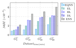
(a) GCD-CPU traces

(b) GCD-Memory traces

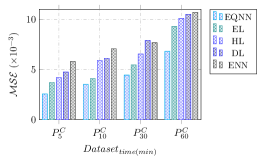
(c) PlanetLab CPU traces

Figure 9: Mean Squared Error

TABLE VIII: Confidence metrics for Mean Squared Error

Dataset	PWSa	Metrics	EQNN	EL	HL	DL	ENN
GCD-CPU	5	EM	5.3012E-06	1.3824E-06	2.3666E-06	1.8460E-06	2.7320E-06
		CI	8.799E-03 - 8.801E-03	1.079E-03 - 1.080E-03	1.169E-03 - 1.170E-03	1.799E-03 - 1.800E-03	2.199E-03 - 2.200E-03
	10	EM	1.7969E-06	3.6608E-06	5.4890E-06	4.5940E-06	3.2681E-06
		CI	1.398E-03 - 1.140E-03	1.992E-03 - 1.993E-03	3.239E-03 - 3.241E-03	3.895E-03 - 3.900E-03	4.599E-03 - 4.600E-03
	30	EM	2.1890E-06	1.4865E-06	6.8200E-05	4.9826E-06	6.8210E-06
		CI	1.298E-03 - 1.299E-03	2.989E-03 - 2.990E-03	3.733E-03 - 3.747E-03	4.179E-03 - 4.180E-03	5.069E-03 - 5.071E-03
	60	EM	1.1743E-06	1.702E-06	6.476E-06	5.8040E-06	8.2199E-06
		CI	2.280E-03 - 2.282E-03	3.798E-03 - 3.801E-03	4.229E-03 - 4.231E-03	4.179E-03 - 4,181E-03	2.39E-05
GCD-Memory	5	EM	5.7890E-05	6.7740E-06	1.7841E-06	8.7341E-06	1.6839E-05
		CI	1.079E-03 - 1.081E-03	1.369E-03 - 1.370E-03	1.919E-03 - 1.920E-03	1.9391E-03 - 1.941E-03	4.090E-03 - 4.093E-03
	10	EM	2.0799E-05	4.0514E-06	4.9616E-06	6.6035E-06	2.5002E-05
		CI	2.507E-03 - 2.512E-03	3.829E-03 - 3.830E-03	3.909E-03 - 3.910E-03	4.099E-03 - 4.101E-03	5.597E-03 - 5.603E-03
	30	EM	6.8200E-05	6.4132E-05	7.1294E-05	5.813E-05	2.5785E-05
		CI	3.329E-03 - 3.331E-03	5.593E-03 - 5.606E-03	6.953E-03 - 6.954E-03	9.307E-03 - 9.310E-03	8.667E-03 - 8.673E-03
	60	EM	4.8290E-05	9.9990E-05	1.5458E-05	2.4786E-06	3.5760E-05
		CI	5.615E-03 - 5.625E-03	6.799E-03 - 6.801E-03	7.818E-03 - 7.822E-03	10.0991E-03 - 10.0996E-03	9.696E-03 - 9.703E-03
PlanetLab CPU	5	EM	4.2810E-06	4.6890E-06	4.6170E-06	6.8910E-06	2.3980E-06
		CI	2.559E-03 - 2.560E-03	3.699E-03 - 3.700E-03	4.199E-03 - 4.200E-03	4.739E-03 - 4.740E-03	5.794E-03 - 5.795E-03
	10	EM	8.4210E-06	9.8140E-06	7.1100E-06	8.7642E-06	1.0890E-05
		CI	3.499E-03 - 3.510E-03	4.092E-03 - 4.093E-03	5.899E-03 - 5.900E-03	6.099E-03 - 6.101E-03	7.058E-03 - 7.061E-03
	30	EM	6.2814E-05	8.6411E-05	1.8230E-05	6.4210E-06	8.6810E-06
		CI	4.423E-03 - 4.436E-03	5.451E-03 - 5.468E-03	6.538E-03 - 6.541E-03	7.899E-03 - 7.900E-03	7.669E-03 - 7.670E-03
	60	EM	8.4210E-05	9.9610E-05	6.4280E-05	2.8136E-05	9.8134E-05
		CI	6.811E-03 - 6.824E-03	9.270E-03 - 9.289E-03	10.075E-03 - 10.088E-03	10.449E-03 - 10.450E-03	10.690E-03 - 10.709E-03

^a PWS: Prediction Window Size, EM: Error Margin, CI: Confidence Interval

9.4.2 Mean Absolute Error

The comparison of resultant values of $\mathcal{MAE}$ obtained for different prediction models over various datasets is presented in Fig. 10. Similar to the $\mathcal{MSE}$, the $\mathcal{MAE}$ values follows the common trend of the performance for all the three evaluated workloads including GCD-CPU (Fig. 10a), GCD-Memory (Fig. 10b), and PL-CPU (Fig. 10c). As depicted in the three aforementioned consequent bar graphs, the $\mathcal{MAE}$ values decreases in the order: EQNN $<$ EL $\leq$ HL $<$ DL $<$ ENN. Further, it is observed that the difference among prediction errors ($\mathcal{MAE}$) is increasing with the growing prediction window-size because of the decrement in the number of training data samples. Hence, it can be concluded that for short-term prediction, all the types of prediction models produces an expected level of prediction accuracy, and the major difference in the performance of prediction arises with the long-term prediction intervals. The reason behind this is that as the number of training samples decreases, there is not enough learning of the patterns and the respective prediction models begins underestimating the relevant information from the training dataset, resulting into a lesser ability of developing necessary correlations and performance degradation with diminished pattern learning.

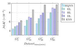
(a) GCD-CPU traces

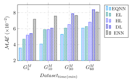
(b) GCD-Memory traces

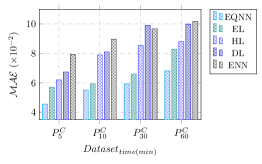
(c) PlanetLab CPU traces

Figure 10: Mean Absolute Error

9.4.3 Training time

The comparison of training-time elapsed during learning process of the various prediction models over distinct workload traces for the prediction window-size of 30 minutes is illustrated in Fig. 11. HL and DL based models consumed similar time of training which is least among the training time of all the prediction models which is due to the usage of Gradient descent and Adam optimizer based training algorithms. While the time elapsed in the training of ENN, EL, and EQNN is longer by reason of usage of evolutionary optimization during learning process. The training time for EL is higher than EQNN and ENN due to the engagement of multiple base prediction models which are simultaneously during the learning process. Contrary to this, the single network based prediction models are used during the learning process of EQNN and ENN, where EQNN consume more time than ENN. The reason behind this is the employment of Qubits and Quantum mechanics based network weight optimization process which uses highly complex computation dealing with complex numbers required for the generation and updation of qubit-based network weights. This discussion concludes the trend for training time: DL $<$ HL$<$ ENN $<$ EQNN $<$ EL. However, the efficiency and applicability of the various prediction models is not affected because the training is a periodic task and can be executed in parallel on the servers equipped with enough resources.

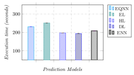
(a) GCD-CPU traces

(b) GCD-Memory traces

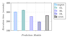
(c) PlanetLab CPU traces

Figure 11: Training time consumption

9.4.4 Absolute Error Frequency

The prediction error achieved for the various comparative models is measured and analysed by evaluating absolute prediction error and comparing its frequency for all three workloads. Fig. 12 compares the frequency of absolute error (Actual value-Predicted value), where EQNN yields least error for the majority of the cloud workloads as compared with the other four types of prediction models. The high frequency of absolute error for a prediction model indicates the consistent potency and stable tendency for yielding maximum prediction accuracy. The absolute error frequency observed for GCD-CPU traces (Fig. 12a), GCD-Memory (Fig. 12b), and PL-CPU traces (Fig. 12c) follows a common trend: ENN $<$ DL $<$ HL $<$ EL $<$ EQNN. The reason behind such a trend is that EQNN employed Qubits population along with evolutionary optimization to allow an improved intuitive learning of patterns which concedes effective learning of extensive range of dynamic workload patterns with optimum accuracy. EL follows EQNN because of the involvement of the learning capability of multiple base predictor models which precisely learns the relevant information from the varying types of workloads. The other prediction models also show slightly lesser but acceptable frequency of prediction error which varies according to the learning capabilities and optimization algorithms involved in their learning process.

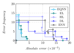
(a) GCD-CPU traces

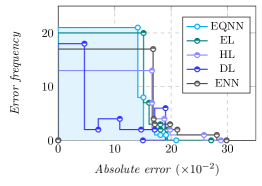
(b) GCD-Memory traces

(c) PlanetLab CPU traces

Figure 12: Absolute Error Frequency

9.5 Trade-offs and Discussion

All the machine learning algorithms have some trade-offs in relation to the adaptive prediction of extensive range of workloads. Likewise, the key difference among various ENNs-based prediction approaches is the evolutionary optimization algorithm applied for the learning process that directly impacts the performance of the prediction approach. The different evolutionary optimization algorithms vary in exploration and exploitation methods involved in the population update process and control parameters tuning process. The evolutionary optimization approach having lesser number of hyperparameters for tuning is more preferable as compared to the one having higher number of tuning hyperparameters. For instance, a Blackhole learning algorithm is a parameterless algorithm having lesser time and space complexity and predicts with higher accuracy than Differential Evolutionary algorithm that involves tuning of hyperparameters including crossover-rate, mutation-rate, learning rate etc. Though the Deep learning approach learns the natural variations of the data samples faster as compared to the evolutionary learning based feed-forward neural network models, they need larger number of data samples for training to estimate the output precisely. Also,deep learning approach having higher complexity computationally, requires expensive GPUs and high processing machines which scales up the cost of their applications. It has been observerd that deep learning algorithms perform better in integration with other machine learning approaches such as random forest for feature extraction and compiles predicted output with the cooperation of the other classification approaches. On the other hand, hybrid and ensemle learning approaches involve combined operation of multiple machine learning algorithms consume higher space and time complexity over the single unit machine learning approaches. Undoubtedly, they adapt to the unseen data and extensive range of workloads with higher efficiency over deep and evolutionary learning approaches because of inclusion of several machine learning approaches at a common platform. Among the hybrid and ensemble learning approaches, the ensemble approach is more adaptable as it considers prediction output from all the considered machine learning algorithms and applies weight optimization for selection of the predicted outcome associated to these learning algorithms while generating the final output. The quantum neural network based learning aproach is most efficient among all the discussed approaches which is validated from the experiments for the accurate prediction of varying workloads. In QNN, the usage of qubits derived from complex numbers having higher diversity over real-numbered network weight values, enables to generate more intuitive pattern and learning of complex relations and helps to predict the output with higher accuracy.

Finally and most important, the diversity of cloud services such as IaaS, PaaS, SaaS, FaaS, etc., has a significant impact while deciding the heterogeneity of approaching workloads, and cloud service provider is bound to provide seamless quality and capacity of resources. There is no perfect guideline to select the best model for a particular cloud service because the resource demands vary dynamically for all the cloud service models. Also, the cloud workloads vary because of various features including resource capacity (viz., CPU, memory, bandwidth, etc.) utilization; priority constraints such as deadline of execution; cost of execution; the amount of variability in the number of job requests over a time period, etc. However, these features (except the amount of variability in the number of job requests over a time period) do not have significant impact on the learning capability of different prediction models because the corresponding data samples are generated periodically, as event recordings for every type of workload, reporting all the relevant information over a timestamp. These data samples are used for training prediction models which show varying accuracy and training computation cost for the estimated workload over the same time period. However, the prediction models can be selected based on the priorities of constraints, such as; for promising high availability and deadline sensitivity, high accuracy prediction models should be selected irrespective of high computation and training time. On the other hand, if there is a constraint of minimum execution cost, the prediction model with lesser computation and training cost is a better option to minimize the processing cost of the respective workload. Further, the workload prediction model can be chosen depending on the diversity of the workloads such as highly random, periodically variable, randomly variable, uniformly or non-uniformly diversifying, etc. Based on the above discussion of the characteristics, design, and capability of the considered machine learning models, it can be postulated that EQNN, Hybrid, and Ensemble models are more suitable for highly random and diversified workloads as they are more capable of learning and handling highly variable and heterogeneous traffic data patterns that involve large amounts of dynamic data, multiple variables with complicated relationships, and even multi-step time series traffic data. While the Evolutionary learning model is preferably suitable for periodically and uniformly variable workload observations recorded sequentially over equal time.

10 Conclusions and Future Directions

This paper presented a comprehensive survey and performance evaluation based comparison of the machine learning based workload prediction models for resource distribution and managemment in cloud environments. The operational design, utility, motivation, and challenges of the workload prediction approach are discussed. Based on the differences in the conceptual and operational characteristics of various prediction models, a classification and taxonomy of machine learning driven prediction models is presented. The leading prediction approaches respective to each prediction model is thoroughly discussed. Further, all the discussed prediction models are implemented on a common platform for an extensive investigation and comparison of the performance of these models. Based on the intensive study and performance evaluation, a trade-off among these prediction models and their applicability are discussed to conclude the holistic study of the cloud workload prediction models. In future, Explainable Artificial Intelligence (XAI) approach can be utilized to build more robust workload prediction models with retraceable mechanism that will help characterize accuracy, transparency, fairness, and prediction outcomes in AI-powered resource management. Further, the efficiency of QNN prediction models can be improved by optimizing the qubit network with a lightweight optimization algorithm and reducing its computational complexity.

Deepika Saxena is a Postdoctoral Research Associate at Goethe University, Frankfurt. She earned her Ph. D. degree from the Department of Computer Applications, National Institute of Technology (NIT), Kurukshetra, India. She received her M.Tech (CSE) degree from Kurukshetra University Kurukshetra, India in 2014. Her major research interests are Neural Networks, Evolutionary Algorithms, Resource Management, and Security in Cloud Computing.

Jitendra Kumar is an Assistant Professor in the Department of Computer Applications, National Institute of Technology Tiruchirappalli, India. He earned his doctorate from the National Institute of Technology Kurukshetra, India in 2019. His current research interests include Cloud Computing, Machine Learning, Data Analytics, Parallel Processing.

Ashutosh Kumar Singh is working as a Professor in the Department of Computer Applications, National Institute of Technology Kurukshetra, India. He has more than 20 years research in various Universities of the India, UK, and Malaysia. He received his PhD from Indian Institute of Technology, BHU, India and Post Doc from Department of Computer Science, University of Bristol, UK. He is also Charted Engineer from UK. His research area includes Verification, Synthesis, Design and Testing of Digital Circuits, Data Science, Cloud Computing, Machine Learning, Security, Big Data.

Stefan Schmid is a Professor at the Technical University of Berlin, Germany, working part-time for the Fraunhofer Institute for Secure Information Technology (SIT) in Germany as well as for the Faculty of Computer Science, the University of Vienna in Austria. MSc and Ph.D. at ETH Zurich, Postdoc at TU Munich and the University of Paderborn, Senior Research Scientist at T-Labs in Berlin, Associate Professor at Aalborg University, Denmark, and Full Professor at the University of Vienna, Austria. He received the IEEE Communications Society ITC Early Career Award 2016 and an ERC Consolidator Grant 2019.

References

- [1] D. Saxena, A. K. Singh, and R. Buyya, “OP-MLB: An online vm prediction based multi-objective load balancing framework for resource management at cloud datacenter,” IEEE Trans. on Cloud Comp., 2021.
- [2] D. Saxena, I. Gupta, J. Kumar, A. K. Singh, and X. Wen, “A secure and multiobjective virtual machine placement framework for cloud data center,” IEEE Systems Journal, 2021.
- [3] R. Mishra, R. Singh, and T. Papadopoulos, “Linking digital orientation and data-driven innovations: A sap-lap linkages framework and research propositions,” IEEE Trans. on Engineering Management, 2022.
- [4] “Cloud comp. market size, share and trends analysis report by service iaas, paas, saas, by deployment public, private, hybrid, by enterprise size, by end use.” Segment Forecasts, 2022-2030.
- [5] Z. Ren, J. Wan, and P. Deng, “Machine-learning-driven digital twin for lifecycle management of complex equipment,” IEEE Trans. on Emerg. Topics in Comp., 2022.
- [6] D. Saxena, A. K. Singh, C.-N. Lee, and R. Buyya, “A sustainable and secure load management model for green cloud data centres,” Scientific Reports, 2023.
- [7] W. Song, Z. Xiao, Q. Chen, and H. Luo, “Adaptive resource provisioning for the cloud using online bin packing,” IEEE Trans. on Computers, vol. 63, no. 11, pp. 2647–2660, 2013.
- [8] D. Saxena and A. Singh, “Security embedded dynamic resource allocation model for cloud data centre,” Elec. Lttr., vol. 56, no. 20, pp. 1062–1065, 2020.
- [9] D. Saxena and A. K. Singh, “Osc-mc: Online secure communication model for cloud environment,” IEEE Comms. Lttr., vol. 25, no. 9, pp. 2844–2848, 2021.
- [10] ——, “Ofp-tm: an online vm failure prediction and tolerance model towards high availability of cloud computing environments,” The Journal of Supercomputing, vol. 78, no. 6, pp. 8003–8024, 2022.
- [11] ——, “A high availability management model based on vm significance ranking and resource estimation for cloud applications,” IEEE Trans. on Services Comp., 2022.
- [12] ——, “Workload forecasting and resource management models based on machine learning for cloud computing environments,” arXiv preprint arXiv:2106.15112, 2021.
- [13] R. Gupta, D. Saxena, I. Gupta, A. Makkar, and A. K. Singh, “Quantum machine learning driven malicious user prediction for cloud network communications,” IEEE Netw. Lttr., 2022.
- [14] X. Wang, L. Ma, X. Wang, Y. Shi, B. Yi, and M. Huang, “Truthful vnfi procurement mechanisms with flexible resource provisioning in nfv markets,” IEEE Trans. on Cloud Comp., 2022.
- [15] D. Saxena and A. K. Singh, “Communication cost aware resource efficient load balancing (care-lb) framework for cloud datacenter,” Recent Advances in Computer Science and Communications, vol. 12, pp. 1–00, 2020.
- [16] A. K. Singh and D. Saxena, “A cryptography and machine learning based authentication for secure data-sharing in federated cloud services environment,” Journal of Applied Security Research, pp. 1–24, 2021.
- [17] D. Saxena and A. K. Singh, “An intelligent traffic entropy learning-based load management model for cloud networks,” IEEE Netw. Lttr., vol. 4, no. 2, pp. 59–63, 2022.
- [18] Y. Xie, L. Pan, S. Yang, and S. Liu, “A random online algorithm for reselling reserved iaas instances in amazon’s cloud marketplace,” IEEE Trans. on Network Science and Engineering, 2022.
- [19] J. Bi, H. Yuan, and M. Zhou, “Temporal prediction of multiapplication consolidated workloads in distributed clouds,” IEEE Trans. on Automation Science and Engineering, 2019.
- [20] H. D. Kabir, A. Khosravi, S. K. Mondal, M. Rahman, S. Nahavandi, and R. Buyya, “Uncertainty-aware decisions in cloud computing: Foundations and future directions,” ACM Comp. Surveys (CSUR), vol. 54, no. 4, pp. 1–30, 2021.
- [21] D. Saxena and A. K. Singh, “A proactive autoscaling and energy-efficient vm allocation framework using online multi-resource neural network for cloud data center,” Neurocomputing, 2020.
- [22] D. Saxena, I. Gupta, A. K. Singh, and C.-N. Lee, “A fault tolerant elastic resource management framework towards high availability of cloud services,” IEEE Trans. on Network and Service Management, 2022.
- [23] D. Saxena and A. K. Singh, “an intelligent security centered resource-efficient resource management model for cloud computing environments,” arXiv preprint arXiv:2210.16602, 2022.
- [24] C. Griner, J. Zerwas, A. Blenk, M. Ghobadi, S. Schmid, and C. Avin, “Cerberus: The power of choices in datacenter topology design-a throughput perspective,” Proceedings of the ACM on Measurement and Analysis of Comp. Systems, vol. 5, no. 3, pp. 1–33, 2021.
- [25] J. Kumar and A. K. Singh, “Workload prediction in cloud using artificial neural network and adaptive differential evolution,” Future Generation Computer Systems, vol. 81, pp. 41–52, 2018.
- [26] J. Kumar, D. Saxena, A. K. Singh, and A. Mohan, “Biphase adaptive learning-based neural network model for cloud datacenter workload forecasting,” Soft Comp., pp. 1–18, 2020.
- [27] J. Kumar, A. K. Singh, and R. Buyya, “Self directed learning based workload forecasting model for cloud resource management,” Information Sciences, vol. 543, pp. 345–366, 2021.
- [28] R. Khorsand, M. Ghobaei-Arani, and M. Ramezanpour, “Fahp approach for autonomic resource provisioning of multitier applications in cloud computing environments,” Software: Practice and Experience, vol. 48, no. 12, pp. 2147–2173, 2018.
- [29] J. Kumar, R. Goomer, and A. K. Singh, “Long short term memory recurrent neural network (lstm-rnn) based workload forecasting model for cloud datacenters,” Procedia Computer Science, vol. 125, pp. 676–682, 2018.
- [30] X. Tang, “Large-scale computing systems workload prediction using parallel improved lstm neural network,” IEEE Access, vol. 7, pp. 40 525–40 533, 2019.
- [31] J. Gao, H. Wang, and H. Shen, “Task failure prediction in cloud data centers using deep learning,” IEEE transactions on services computing, 2020.
- [32] L. Ruan, Y. Bai, S. Li, S. He, and L. Xiao, “Workload time series prediction in storage systems: a deep learning based approach,” Cluster Comp., pp. 1–11, 2021.
- [33] L. Ruan, Y. Bai, S. Li, J. Lv, T. Zhang, L. Xiao, H. Fang, C. Wang, and Y. Xue, “Cloud workload turning points prediction via cloud feature-enhanced deep learning,” IEEE Trans. on Cloud Comp., 2022.
- [34] S. Tuli, S. S. Gill, P. Garraghan, R. Buyya, G. Casale, and N. Jennings, “Start: Straggler prediction and mitigation for cloud comp. environments using encoder lstm networks,” IEEE Trans. on Serv. Comp., 2021.
- [35] Q. Zhang, L. T. Yang, Z. Yan, Z. Chen, and P. Li, “An efficient deep learning model to predict cloud workload for industry informatics,” IEEE Trans. on Industrial Informatics, vol. 14, no. 7, pp. 3170–3178, 2018.
- [36] Z. Chen, J. Hu, G. Min, A. Y. Zomaya, and T. El-Ghazawi, “Towards accurate prediction for high-dimensional and highly-variable cloud workloads with deep learning,” IEEE Trans. on Parallel and Distributed Systems, vol. 31, no. 4, pp. 923–934, 2019.
- [37] C. Peng, Y. Li, Y. Yu, Y. Zhou, and S. Du, “Multi-step-ahead host load prediction with gru based encoder-decoder in cloud computing,” in 2018 10th International Conference on Knowledge and Smart Technology (KST). IEEE, 2018, pp. 186–191.
- [38] F. Qiu, B. Zhang, and J. Guo, “A deep learning approach for vm workload prediction in the cloud,” in 2016 17th IEEE/ACIS Inter. Conf. on Software Engineering, Artificial Intelligence, Networking and Parallel/Distributed Comp. (SNPD). IEEE, 2016, pp. 319–324.
- [39] W. Zhang, P. Duan, L. T. Yang, F. Xia, Z. Li, Q. Lu, W. Gong, and S. Yang, “Resource requests prediction in the cloud computing environment with a deep belief network,” Software: Practice and Experience, vol. 47, no. 3, pp. 473–488, 2017.
- [40] Y. Wen, Y. Wang, J. Liu, B. Cao, and Q. Fu, “Cpu usage prediction for cloud resource provisioning based on deep belief network and particle swarm optimization,” Concurrency and Computation: Practice and Experience, vol. 32, no. 14, p. e5730, 2020.
- [41] M. Xu, C. Song, H. Wu, S. S. Gill, K. Ye, and C. Xu, “Esdnn: Deep neural network based multivariate workload prediction approach in cloud environment,” arXiv preprint arXiv:2203.02684, 2022.
- [42] P. Bhagtya, S. Raghavan, and K. Chandraseakran, “Workload classification in multi-vm cloud environment using deep neural network model,” in Proceedings of the 36th Annual ACM Symposium on Applied Comp., 2021, pp. 79–82.
- [43] Y. Li, H. Hu, Y. Wen, and J. Zhang, “Learning-based power prediction for data centre operations via deep neural networks,” in Proceedings of the 5th International Workshop on Energy Efficient Data Centres, 2016, pp. 1–10.
- [44] J. Bi, S. Li, H. Yuan, Z. Zhao, and H. Liu, “Deep neural networks for predicting task time series in cloud computing systems,” in 2019 IEEE 16th International Conference on Networking, Sensing and Control (ICNSC). IEEE, 2019, pp. 86–91.
- [45] S. Kardani-Moghaddam, R. Buyya, and K. Ramamohanarao, “Adrl: A hybrid anomaly-aware deep reinforcement learning-based resource scaling in clouds,” IEEE Trans. on Parallel and Distributed Systems, vol. 32, no. 3, pp. 514–526, 2020.
- [46] M. E. Karim, M. M. S. Maswood, S. Das, and A. G. Alharbi, “Bhyprec: A novel bi-lstm based hybrid recurrent neural network model to predict the cpu workload of cloud virtual machine,” IEEE Access, vol. 9, pp. 131 476–131 495, 2021.
- [47] J. Bi, S. Li, H. Yuan, and M. Zhou, “Integrated deep learning method for workload and resource prediction in cloud systems,” Neurocomputing, vol. 424, pp. 35–48, 2021.
- [48] Z. Chen, Y. Zhu, Y. Di, and S. Feng, “Self-adaptive prediction of cloud resource demands using ensemble model and subtractive-fuzzy clustering based fuzzy neural network,” Computational intelligence and neuroscience, vol. 2015, 2015.
- [49] C. Liu, C. Liu, Y. Shang, S. Chen, B. Cheng, and J. Chen, “An adaptive prediction approach based on workload pattern discrimination in the cloud,” Journal of Network and Computer Applications, vol. 80, pp. 35–44, 2017.
- [50] M. N. H. Shuvo, M. M. S. Maswood, and A. G. Alharbi, “Lsru: A novel deep learning based hybrid method to predict the workload of virtual machines in cloud data center,” in 2020 IEEE Region 10 Symposium (TENSYMP). IEEE, 2020, pp. 1604–1607.
- [51] N. Singh and S. Rao, “Ensemble learning for large-scale workload prediction,” IEEE Trans. on Emg. Topics in Comp., vol. 2, no. 2, pp. 149–165, 2014.
- [52] B. Feng, Z. Ding, and C. Jiang, “Fast: A forecasting model with adaptive sliding window and time locality integration for dynamic cloud workloads,” IEEE Trans. on Serv. Comp., 2022.
- [53] I. K. Kim, W. Wang, Y. Qi, and M. Humphrey, “Forecasting cloud application workloads with cloudinsight for predictive resource management,” IEEE Trans. on Cloud Comp., 2020.
- [54] W. Iqbal, J. L. Berral, A. Erradi, D. Carrera et al., “Adaptive prediction models for data center resources utilization estimation,” IEEE Trans. on Network and Service Management, vol. 16, no. 4, pp. 1681–1693, 2019.
- [55] J. Kumar, A. K. Singh, and R. Buyya, “Ensemble learning based predictive framework for virtual machine resource request prediction,” Neurocomputing, vol. 397, pp. 20–30, 2020.
- [56] A. K. Singh, D. Saxena, J. Kumar, and V. Gupta, “A quantum approach towards the adaptive prediction of cloud workloads,” IEEE Trans. on Parallel and Distributed Systems, 2021.
- [57] J. J. Prevost, K. Nagothu, B. Kelley, and M. Jamshidi, “Prediction of cloud data center networks loads using stochastic and neural models,” in 2011 6th International Conference on System of Systems Engineering. IEEE, 2011, pp. 276–281.
- [58] D. Saxena and A. K. Singh, “Auto-adaptive learning-based workload forecasting in dynamic cloud environment,” International Journal of Computers and Applications, pp. 1–11, 2020.
- [59] J. Kumar and A. K. Singh, “Dynamic resource scaling in cloud using neural network and black hole algorithm,” in 2016 Fifth International Conference on Eco-friendly Comp. and Communication Systems (ICECCS). IEEE, 2016, pp. 63–67.
- [60] W. Zhang and P. Duan, “Towards a deep belief network-based cloud resource demanding prediction,” in 2015 IEEE 12th Intl Conf on Ubiquitous Intelligence and Comp. and 2015 IEEE 12th Intl Conf on Autonomic and Trusted Comp. and 2015 IEEE 15th Intl Conf on Scalable Comp. and Communications and Its Associated Workshops (UIC-ATC-ScalCom). IEEE, 2015, pp. 1043–1048.
- [61] D. Chen, X. Zhang, L. L. Wang, and Z. Han, “Prediction of cloud resources demand based on hierarchical pythagorean fuzzy deep neural network,” IEEE Trans. on Serv. Comp., 2019.
- [62] K. Qazi and I. Aizenberg, “Cloud datacenter workload prediction using complex-valued neural networks,” in 2018 IEEE Second International Conference on Data Stream Mining & Processing (DSMP). IEEE, 2018, pp. 315–321.
- [63] J. L. H. C. Reiss, J. Wilkes, “Google–cluster traces:format+schema,” Google Inc., White Paper, 2011.
- [64] A. Beloglazov and R. Buyya, “Optimal online deterministic algorithms and adaptive heuristics for energy and performance efficient dynamic consolidation of virtual machines in cloud data centers,” Concurrency and Computation: Practice and Experience, vol. 24, no. 13, pp. 1397–1420, 2012.