Seiberg Duality conjecture for star-shaped quivers and finiteness of Gromov-Witten thoery for D-type quivers

Abstract

This is the second work on Seiberg Duality. This work proves that the Seiberg duality conjecture holds for star-shaped quivers: the Gromov-Witten theories for two mutation-related varieties are equivalent.

In particular, it is known that a $D$-type quiver goes back to itself after finite times quiver mutations, and we further prove that Gromov-Witten theory together with kähler variables of a $D_{3}$-type quiver variety return to the original ones after finite times quiver mutations.

1 Introduction

The equivalence of 2d quantum field theories is a longstanding interesting topic in mathematical physics, including the following two examples: (1)the equivalence between Gromov-Witten theories under K-equivariant birational transformation [LR01, LLW10, Rua06, BG09, CIJ18, EW12]; (2)the Landau-Ginzburg/Calabi-Yau correspondence (equivalence between Gromov-Witten theory of CY hypersurface and Fan-Jarivs-Ruan-Witten theory of a Landau-Ginzburg model) [CR10, CIR14, IMRS21].

1. A vast class of birational transformation comes from the variation of the GIT quotient. Explicitly, we consider an Artin stack $[V/G]$, where $V$ is some affine space and $G$ is a torus. The space of stability condition $\mathfrak{M}$ is decomposed into chambers called phases. Different phase determines different semistable locus $V^{ss}\subseteq V$ and gives us different GIT quotients $[V^{ss}/G]$ (a toric DM stack). Two such GIT quotients are connected by a birational transformation. Furthermore, if the birational transformation is K-equivariant, "crossing the wall" of two phases will preserve the Gromov-Witten theories of the two different corresponding GIT quotients [CIJ18, EW12].

2. The LG/CY correspondence is quite similar, which, when we put it into a global picture, constitutes the so-called gauge linear sigma model (GLSM). GLSM is a 2d quantum field theory introduced by Witten in [Wit97], and its mathematical theory is developed in [FJR18, KL18, CFFG⁺18, FK20]. Consider a stack $[V/G]$ with a potential function $W$, where $V$ is some affine space, and $G$ is a reductive algebraic group. We consider phases corresponding to different stability conditions on $[V/G]$. In the geometric (affine LG) phase, the GLSM typically corresponds to Gromov-Witten theory (FJRW theory). Crossing the wall of those two phases, we obtain the equivalence of GW and FJRW theories.

The examples described above both focus on a GIT quotient $[V\sslash G]$ (and its complete intersection) where the gauge group $G$ is abelian. Meanwhile, there are many essential and exciting GIT quotients where $G$ is nonabelian, such as quiver varieties and their complete intersections. A natural question arises: is there any equivalence of gauge theories for nonabelian GIT quotients? Seiberg Duality gives a positive answer to the above question.

The fascinating Seiberg duality conjecture asserts the equivalence of gauge theories of two quivers related by a quiver mutation. Usually, such two quivers are not simply related by a phase transition. This topic is vastly investigated in the physics literature, but less is known in math. See [Hor13, HT07, BPZ15, GLF16] for physics achievements. Nevertheless, there is a mathematical conjecture proposed by Yongbin Ruan for the 2d Seiberg Duality [Rua17], and we attempted it in previous work by checking the linear quivers, see [Don20, Zha21]. Although this work is one piece of a series work, We try to make it self-contained.

1.1 Introduction to Seiberg duality conjecture

We start from a quiver $(Q_{f}\subset Q_{0},Q_{1},W)$, where $Q_{0}$ is the set of nodes, $Q_{f}$ is the set of framed nodes, $Q_{0}\backslash Q_{f}$ is the set of gauged nodes, $Q_{1}$ is the set of arrows, and $W$ is a potential function. We usually denote the arrows from node $i$ to node $j$ by $i\rightarrow j$ and denote the number of such arrows between the two nodes by $b_{ij}$. We assume that arrows between two nodes are in a unique direction. Such quivers are called cluster quivers [Kir16].

Assign an integer vector $\vec{v}=(N_{i})_{i\in Q_{0}}$ to the quiver, one integer to a node. Let $V=\oplus_{i\rightarrow j}\mathbb{C}^{N_{i}\times N_{j}}$, $G=\prod_{i\in Q_{0}\backslash Q_{f}}GL(N_{i})$, and $\theta\in\chi(G)$, and then we get an input data $(V,G,\theta)$ for a GIT quotient $V\sslash_{\theta}G$, which is defined to be the quiver variety, see Definition 2.2. For each node $k$, define the outgoing to be $N_{f}(k):=\sum_{k\rightarrow j}b_{kj}N_{j}$ and the incoming to be $N_{a}(k):=\sum_{i\rightarrow k}b_{ik}N_{i}$.

Performing a quiver mutation as Definition 2.8 at a gauge node $k$ (we will reserve this small letter $k$ for the node we perform a quiver mutation at), we obtain a new quiver $(\tilde{Q}_{f}\subset\tilde{Q}_{0},\tilde{Q}_{1},\tilde{W})$ together with the assigned integer vector $\vec{v}^{\prime}$. Whenever there is a pair of opposite arrows between two nodes arising from quiver mutation, we have to annihilate them and denote the number of annihilated pairs by $a_{ij}$. Hence, we still get a cluster quiver after a quiver mutation. Denote the input data of the GIT quotient by $(\tilde{V},\tilde{G},\tilde{\theta})$. For adequately chosen phases $\theta$ and $\tilde{\theta}$ of the two mutation-related quivers, we consider the critical locus of $\{dW=0\}\sslash_{\theta}G$ and $\{d\tilde{W}=0\}\sslash_{\theta}G$, which we denote by $\mathcal{Z}$ and $\tilde{\mathcal{Z}}$ respectively.

We will consider Gromov-Witten theories of $\mathcal{Z}$ and $\tilde{\mathcal{Z}}$. Roughly, genus $g$ Gromov-Witten theory counts the genus-$g$ curves of some degree in the target variety. Let $\mathcal{F}_{g}^{\mathcal{Z}}(\vec{q})$ and $\mathcal{F}_{g}^{\tilde{\mathcal{Z}}}(\vec{q}^{\prime})$ denote the generating series of Gromov-Witten invariants of $\mathcal{Z}$ and $\tilde{\mathcal{Z}}$ of genus $g$, with $\vec{q}$ and $\vec{q}^{\prime}$ their kähler variables. The 2d Seiberg Duality Conjecture is stated as follows.

Conjecture 1.1 ([Rua17, BPZ15]).

$$\mathcal{F}_{g}^{\mathcal{Z}}(\vec{q})=\mathcal{F}_{g}^{\tilde{\mathcal{Z}}}(\vec{q}^{\prime})\,,$$ (1.1)

and kähler variables transform as: $q_{k}^{\prime}=q_{k}^{-1}$, and for $i\neq k$,

• if $N_{f}(k)>N_{a}(k)$, $\frac{{e}^{\pi i(N_{f}(j)^{\prime}-1)}q_{j}^{\prime}}{{e}^{\pi i(N_{f}(j)-1)}q_{j}}=({e}^{\pi iN_{k}^{\prime}}q_{k})^{[b_{kj}]_{+}}({e}^{\pi iN_{k}^{\prime}})^{[-b_{kj}]_{+}}\prod_{i\neq k}e^{\pi iN_{i}a_{ij}}$;

• if $N_{f}(k)=N_{a}(k)$, $\frac{{e}^{\pi i(N_{f}(j)^{\prime}-1)}q_{j}^{\prime}}{{e}^{\pi i(N_{f}(j)-1)}q_{j}}=\left(\frac{{e}^{\pi iN_{k}^{\prime}}q_{k}}{1+(-1)^{N_{k}^{\prime}}q_{k}}\right)^{[b_{kj}]_{+}}\left({e}^{\pi iN_{k}^{\prime}}(1+(-1)^{N_{k}^{\prime}}q_{k})\right)^{[-b_{kj}]_{+}}\prod_{i\neq k}e^{\pi iN_{i}a_{ij}}$.

• If $N_{f}(k)<N_{a}(k)$, $\frac{{e}^{(N_{f}(j)^{\prime}-1)}q_{j}^{\prime}}{{e}^{(N_{f}(j)-1)}q_{j}}=({e}^{\pi iN_{k}^{\prime}})^{[b_{kj}]_{+}}\left({e}^{\pi i(N_{f}(k)-N_{k})}q_{k}\right)^{-[-b_{kj}]_{+}}\prod_{i\neq k}e^{\pi iN_{i}a_{ij}}$

where $a_{ij}$ denotes the number of “annihilated” 2-cycles between the nodes i and j in the quiver mutation, $[b]_{+}=\max\{b,0\}$.

We will first focus on the genus-zero version of the Conjecture. The genus zero wall-crossing Theorem states that the (equivariant) $\mathcal{J}$-function, which comprises all genus zero GW invariants, is equal to the (equivariant) quasimap $I$-function under the mirror map, see [CFK14]. Hence, we move to the quasimap theory [CFKM14][CCFK15] and investigating the relations between the quasimap $I$-functions. Assume that both $\mathcal{Z}$ and $\tilde{\mathcal{Z}}$ admit a good torus action S. Denote their equivariant quasimap small $I$-functions by $I^{{\mathcal{Z},S}}(q)$ and $I^{\tilde{\mathcal{Z}},S}(\vec{q}^{\prime})$.

Our previous work proves the Conjecture for $A_{n}$-type quiver [Zha21] by proving that the equivariant quasimap small $I$-function of a flag variety keeps unchanged under a quiver mutation at a node $k$ with the expected transformation on kähler variables.

The first goal of this work is to extend our result from $A$-type quivers to a star-shaped quiver,

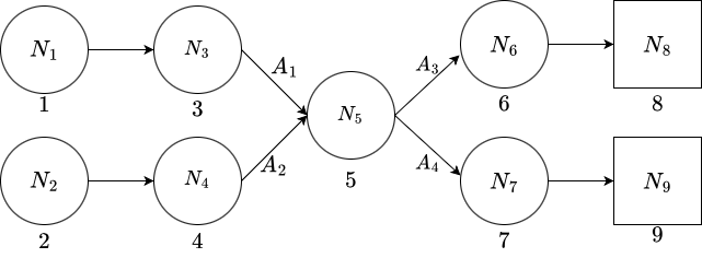
Figure 1: A star-shaped quiver with additional conditions on $N_{i}$ as Example 2.7

In particular, the Seiberg Duality Conjecture holds for $D,\,E$-type quivers if we view them as special star-shaped quivers.

By [FZ03], the quiver diagrams of $A,\,D,\,E$ return to the original ones after finite times quiver mutations, and their cluster algebras are finite. So the second goal is to investigate how Gromov-Witten theories of those mutation-related quivers are related: whether the Gromov-Witten theory of one quiver including its kähler variables returns to the original ones after a finite number of quiver mutations. We will take a $D_{3}$-type quiver as an example to explicitly display the finiteness.

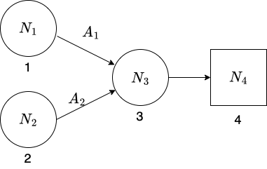
Figure 2: The graph of the $D_{3}$ quiver. The numerals below the nodes are used to label nodes. Assumptions $N_{4}=N_{1}+N_{2},\,N_{4}>N_{3},\,N_{3}>N_{1},\,N_{3}>N_{2}\,$ are made.

We want to emphasize that the finiteness is neither trivial nor general, and we refer readers to [BPZ15] for an example whose kähler variables cannot go back to the original ones.

1.2 Main Theorems

1.2.1 Seiberg Duality conjecture for a star-shaped quiver

Consider a star-shaped quiver first as Figure 1. For a chosen phase as Equation (2.7), we can define a quiver variety and denote it by $\mathcal{X}_{s}$. Performing a quiver mutation $\mu_{5}$ at the center node $5$, we obtain the quiver diagram below with a potential function $\widetilde{W}_{s}=tr(A_{3}B_{1}A_{5})+tr(A_{3}B_{3}A_{6})+tr(A_{4}B_{2}A_{5})+tr(A_{4}B_{4}A_{6})$.

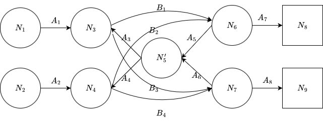
Figure 3: $N_{5}^{\prime}=N_{6}+N_{7}-N_{5}$.

For a carefully chosen phase (geometric phase) (2.12), we get the critical locus of the potential function, $\tilde{\mathcal{Z}}_{s}:=(d\widetilde{W}_{s}=0)\sslash_{\tilde{\theta}_{s}}\tilde{G}_{s}$. Both $\mathcal{X}_{s}$ and $\tilde{\mathcal{Z}_{s}}$ admit a good torus action $S=(\mathbb{C}^{*})^{N_{7}+N_{8}}$ which ats on matrices $A_{7},A_{8}$ from the right naturally.

Theorem 1.2.

The quiver mutation $\mu_{5}$ preserves the equivariant quasimap small $I$ functions in the following sense.

1. When $N_{6}+N_{7}\geq N_{3}+N_{4}+2$,

   $$I^{\mathcal{X}_{s},S}(\vec{q})=I^{\tilde{\mathcal{Z}_{s}},S}(\vec{q}^{\prime})\,,$$ (1.2)

   and the map between the kähler variables is

   $$q_{5}^{\prime}=q_{5}^{-1},\,q_{6}^{\prime}=q_{6}q_{5},\,q_{7}^{\prime}=q_{7}q_{5},\,q_{i}^{\prime}=q_{i},\text{ for }i\neq 5,6,7\,.$$ (1.3)

2. When $N_{6}+N_{7}=N_{3}+N_{4}+1$,

   $$I^{\mathcal{X}_{s},S}(\vec{q})=e^{(-1)^{N_{5}^{\prime}}q_{5}}I^{{\tilde{\mathcal{Z}}_{s}},S}(\vec{q}^{\prime})\,,$$ (1.4)

   and the map between kähler variables is the same with (1.3).

3. When $N_{6}+N_{7}=N_{3}+N_{4}$,

   $$I^{\mathcal{X}_{s},S}(\vec{q})=(1+(-1)^{N_{5}^{\prime}}q_{5})^{N_{5}^{\prime}}I^{{\tilde{\mathcal{Z}}_{s}},S}(\vec{q}^{\prime})\,,$$ (1.5)

   and the map between kähler variables is

   $$q_{3}^{\prime}=q_{3}(1+(-1)^{N_{5}^{\prime}}q_{5})\,,q_{4}^{\prime}=q_{4}(1+(-1)^{N_{5}^{\prime}}q_{5})\,,q_{5}^{\prime}=q_{5}^{-1}\,,$$

   $$q_{6}^{\prime}=\frac{q_{6}q_{5}}{(1+(-1)^{N_{5}^{\prime}}q_{5})}\,,q_{7}^{\prime}=\frac{q_{7}q_{5}}{(1+(-1)^{N_{5}^{\prime}}q_{5})}\,,q_{i}^{\prime}=q_{i},\text{ for }i=1,2\,.$$ (1.6)

Remark 1.3.

The above theorem can be extended to any star-shaped quiver with an arbitrary number of incoming arrows and outgoing arrows without potential. However, one has to be careful about the change of the phases under mutation when explicitly construct the varieties after the quiver mutation. The transformation of phases is inspired by the sphere partition function in the physics literature.

The $D_{3}$-type quiver in Figure 2 is a special case of a star-shaped quiver with only one arrow starting from the center node. Denote the quiver variety of the $D_{3}$ type quiver by $\mathcal{X}_{0}$. Performing a quiver mutation $\mu_{3}$ to the $D_{3}$-quiver, we obtain the quiver diagram below.

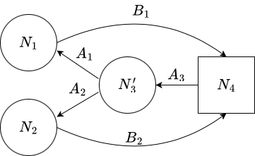
Figure 4: The quiver diagram obtained by performing a quiver mutation $\mu_{3}$ to the quiver in Figure 2. It has a potential function $W=tr(A_{1}B_{1}A_{3})+tr(A_{2}B_{2}A_{3})$.

Under suitable phase (2.17), we get the critical locus of the potential, which is a complete intersection in another quiver variety and is denoted by $\mathcal{Z}_{1}$. See Example 2.10. Both $\mathcal{X}_{0}$ and $\mathcal{Z}_{1}$ admit a good torus action $S^{1}=(\mathbb{C}^{*})^{N_{4}}$. Let $I^{\mathcal{X}_{0},S^{1}}(\vec{q})$ and $I^{\mathcal{Z}_{1},S^{1}}(\vec{q}^{\prime})$ be the equivariant quasimap small $I$-functions of varieties $\mathcal{X}_{0}$ and $\mathcal{Z}_{1}$. The equivariant quasimap small $I$-functions of $\mathcal{X}_{0}$ and $\mathcal{Z}_{1}$ satisfy the same relation with Theorem 1.2 item $(c)$.

Corollary 1.4.

$$I^{\mathcal{X}_{0},S^{1}}(\vec{q})=(1+(-1)^{N_{3}^{\prime}}q_{3})^{\sum_{I=1}^{N_{1}}x_{I}+\sum_{I=1}^{N_{2}}y_{I}-\sum_{F}^{N_{3}}\lambda_{F}+N_{3}^{\prime}}I^{\mathcal{Z}_{1},S^{1}}(\vec{q}^{\prime})\,,$$ (1.7)

and the transformation of kähler variables is as follows,

$$q_{1}^{\prime}=(1+(-1)^{N_{3}^{\prime}}q_{3})q_{1},\,q_{2}^{\prime}=(1+(-1)^{N_{3}^{\prime}}q_{3})q_{2},\,q_{3}^{\prime}=q_{3}^{-1}\,.$$ (1.8)

1.2.2 Finiteness of the Gromov-Witten theories of $D_{3}$-quivers

Although Gromov-Witten theories are preserved at each step, it is unknown whether kähler variables go back to the original ones after a finite number of quiver mutations. Our next result proves that it can be true in some cases.

Theorem 1.5.

Perform quiver mutations $\mu_{3}\rightarrow\mu_{1}\rightarrow\mu_{2}$ to the $D_{3}$-quiver several times, we can prove that the Gromov-Witten theory together with kähler variables go back to those of the $D_{3}$-quiver. Explicitly, let $(q_{1},q_{2},q_{3})$ be the kähler variables of a $D_{3}$ quiver variety. Then its kähler variables transform as the following table, and the concrete relation of $I$-functions can be found in the last sub-section.

Mutation	varieties	1st node	2nd node	3rd node
	$\mathcal{X}_{0}$	$q_{1}$	$q_{2}$	$q_{3}$
$\mu_{3}$	$\mathcal{Z}_{1}$	$(1+(-1)^{N_{3}^{\prime}}q_{3})q_{1}$	$(1+(-1)^{N_{3}^{\prime}}q_{3})q_{2}$	$q_{3}^{-1}$
$\mu_{1}$	$\mathcal{Z}_{2}$	$(1+(-1)^{N_{3}^{\prime}}q_{3})^{-1}q_{1}^{-1}$	$(1+(-1)^{N_{3}^{\prime}}q_{3})q_{2}$	$q_{3}^{-1}$
$\mu_{2}$	$\mathcal{Z}_{3}$	$((1+(-1)^{N_{3}^{\prime}}q_{3})q_{2})^{-1}$	$((1+(-1)^{N_{3}^{\prime}}q_{3})q_{1})^{-1}$	$q_{3}$
$\mu_{3}$	$\mathcal{X}_{4}$	$q_{2}^{-1}$	$q_{1}^{-1}$	$q_{3}^{-1}$
$\mu_{1}$	$\mathcal{X}_{5}$	$q_{2}$	$q_{1}^{-1}$	$q_{3}^{-1}q_{2}^{-1}$
$\mu_{2}$	$\mathcal{X}_{6}$	$q_{2},$	$q_{1}$	$q_{3}^{-1}q_{2}^{-1}q_{1}^{-1}$
$\mu_{3}$	$\mathcal{X}_{7}$	$q_{2}^{-1}$	$q_{1}^{-1}$	$q_{1}q_{2}q_{3}$
$\mu_{1}$	$\mathcal{X}_{8}$	$q_{2}$	$q_{1}^{-1}$	$q_{1}q_{3}$
$\mu_{2}$	$\mathcal{X}_{9}$	$q_{2}$	$q_{1}$	$q_{3}$

Table 1: kähler variables’ transformations.

Furthermore, we have the following byproduct. Our previous work only focused on the $A_{n}$-type quiver, and one side of the two mutation-related quivers has no potential. It is also interesting to know how to deal with the mutation when there are non-trivial potentials on two sides of a quiver mutation. In the process of quiver mutations to recover $D_{3}$, we will encounter this situation. See Example 2.11 and Example 2.12.

An unexpected phenomenon is that in recovering the original Gromov-Witten theory of $D_{3}$, the kähler variables do not always change as the Seiberg duality conjecture asserts. It is due to the choices of phases for quivers appearing in this process. For nonabelian GIT quotient $[V\sslash_{\theta}G]$, it is highly possible that it is not an algebraic variety and the good phase for an algebraic variety is not for Seiberg Duality. Nevertheless, we can still prove that Gromov-Witten theories of constructed varieties are equivalent under some unusual transformations on kähler variables. See Remark 5.8.

Furthermore, for the ADE type quiver varieties, it is expected that their quantum cohomology rings admit finite cluster algebra structure, see [FZ02, FZ03, BFZ05, FZ07, DWZ08, DWZ10] for the theory of cluster algebras and [BPZ15] for the physics expectation on the cluster algebra structure on quantum cohomology rings. Our work on the cluster algebra structure for quantum cohomology rings of $A_{n}$-type quivers is in progress.

1.3 Ideas for proofs

The key is that Seiberg duality is a local behavior: it only affects the behavior of nodes and arrows around the node $k$. Let us consider a fundamental building block.

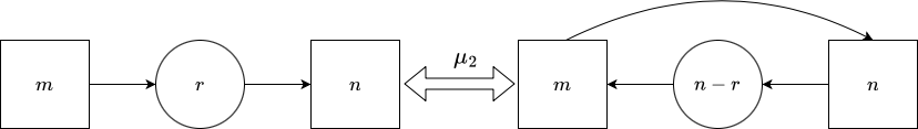
Figure 5: Two quiver diagrams related by a quiver mutation at the center node. We require that $n\geq m$.

The quiver variety of the left-hand side is the total space of $m$-copies of tautological bundles over a Grassmannian $S^{\oplus m}\rightarrow Gr(r,n)$. The variety for the right-hand side is the total space of the $m$-copies of the dual of the tautological bundle over the dual Grassmannian $(S^{\vee})^{\oplus m}\rightarrow Gr(n-r,n)$. There is a common torus $S^{2}=(\mathbb{C}^{*})^{m+n}$ action on the two varieties, and one can find that the numbers of torus fixed points are equal. Let $I^{Gr,S^{2}}(q)$ and $I^{Gr^{\vee},S^{2}}(q^{\prime})$ denote their equivariant quasimap small $I$-functions.

Theorem 1.6 ([Don20, BPZ15]).

1. When $n\geq m+2$, ${I}^{Gr,S^{2}}(q)={I}^{Gr^{\vee},S^{2}}(q^{-1})$.

2. When $n=m+1$, ${I}^{Gr,S^{2}}(q)={e}^{(-)^{n-r}q}\,{I}^{Gr^{\vee},S^{2}}(q^{-1})$.

3. When $n=m$, ${I}^{Gr,S^{2}}(q)=(1+(-1)^{n-r}q)^{\sum_{A=1}^{m}\eta_{A}-\sum_{F=1}^{n}\lambda_{F}+n-r}{I}^{Gr^{\vee},S^{2}}(q^{-1})$ .

In the formula, $\eta_{A}$ for $A=1,\ldots,m$ are equivariant parameters of $(\mathbb{C}^{*})^{m}$ action on the fiber and $\lambda_{F}$ for $F=1,\ldots,n$ are equivariant parameters for $(\mathbb{C}^{*})^{n}$ action on Grassmannian.

The idea for proving the equivalence between $I^{\mathcal{X}_{s}}$ and $I^{\tilde{\mathcal{Z}_{s}}}$ is to freeze the nodes that are related to the center nodes as shown in the following Figure 6.

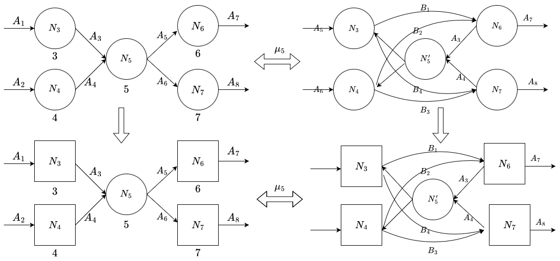
Figure 6: From the left to the right, we perform the quiver mutation at the center node, and from top to bottom, we freeze the adjacent nodes.

The two quiver diagrams on the bottom of the above Figure 6 are the two quivers in Figure 5 with outgoing $n=N_{7}+N_{8}$ and incoming $m=N_{3}+N_{4}$. Correspondingly, by some non-trivial combinatorics, we can isolate the terms in $I$-functions of the adjacent nodes and reduce the equivalence between $I^{\mathcal{X}_{s},S^{1}}$ and $I^{\tilde{\mathcal{Z}_{1}},S^{1}}$ to the equivalence between $I^{Gr,S^{2}}$ and $I^{Gr^{\vee},S^{2}}$, which is done.

The proof for the Theorem 1.5 is almost the same, and the difficulty there is how to choose appropriate phases for each quiver so that we can identify their $I$-functions, one can consult the proof in Section 5.

2 Introduction to the quiver variety and quiver mutation

In Section 2.1, we will introduce the basic definition for quiver varieties, including prominent examples like general star-shaped-quiver and $D_{3}$-quiver varieties. We refer readers to the excellent book [Kir16] for an introduction to quiver varieties. In Section 2.2, we will introduce the quiver mutation and perform quiver mutations to the center node of a general star-shaped quiver and to a $D_{3}$-quiver multiple times. We will then construct the corresponding varieties for all quivers we get. In this process, the transformations of phases and potentials are inspired by the computation of the so-called sphere partition functions [BPZ15, Section 3 ].

2.1 Quiver varieties

An input data of a GIT quotient consists of the following ingredients:

1. an affine algebraic variety $V=\operatorname{Spec}(A)$ over $\mathbb{C}$ with at most lci singularities;

2. a connected reductive algebraic group $G$ acting on $V$;

3. a character $\theta$ in the character group of $G$ denoted by $\chi(G):=\operatorname{Hom}(G,\mathbb{C}^{*})$.

Each character $\theta\in\chi(G)$ determines an one-dimensional representation $\mathbb{C}_{\theta}$ of $G$ and a line bundle over $V$,

$$L_{\theta}:=V\times\mathbb{C}_{\theta}\in\text{Pic}^{G}(V)\,.$$ (2.1)

Definition 2.1.

Given an input data $(V,G,\theta)$, $x\in V$ is called $\theta$-semistable if $\exists\,k>0$ and $s\in{H}^{0}(V,{L}_{\theta}^{k})^{G}$, such that $s(x)\neq 0$ and every $G$-orbit in $D_{s}=\{s\neq 0\}$ is closed. Further, a $\theta$-semistable point $x\in V$ is called $\theta$-stable if its stabilizer $\operatorname{Stab}_{G}(x)=\{g\in G,g\cdot x=x\}$ is finite. Let $V^{ss}_{\theta}(G)$ denote the set of semistable points, $V^{s}_{\theta}(G)$ the set of stable points, and $V^{us}_{\theta}(G)$ the set of unstable points. The GIT quotient of $(V,G,\theta)$ is defined as $V\sslash_{\theta}G:=V^{ss}_{\theta}(G)/G$.

The following will be assumed throughout.

1. $V^{s}=V^{ss}\neq\emptyset$.

2. The subscheme $V^{s}$ is nonsingular.

3. The group $G$ acts freely on $V^{s}$.

Therefore, the GIT quotient $V\sslash_{\theta}G$ is smooth. We will instead denote the set of semistable points, the set of stable points, and the set of unstable points by $V^{ss}(G)$, $V^{s}(G)$, and $V^{us}(G)$, and denote the GIT quotient of $(V,G,\theta)$ by $V\sslash G$ when there is no confusion arising for the character.

Definition 2.2 ([Kir16]).

A quiver diagram is a finite oriented graph consisting of $(Q_{f}\subset Q_{0},Q_{1},W)$ where

• $Q_{0}$ is the set of vertices among which $Q_{f}$ is the set of frame (frozen) nodes, usually denoted by in the graph, and $Q_{0}\backslash Q_{f}$ is the set of gauge nodes, usually denoted by $\bigcirc$;

• $Q_{1}$ is the set of arrows; an arrow from nodes $i$ to $j$ is usually denoted by $i\rightarrow j\in Q_{1}$, and the number of such arrows is denoted by $b_{ij}$;

• $W$ is the potential function, defined as a function on cycles in the diagram.

We always assume that the quiver diagram has no $1$-cycle or $2$-cycles, known as the cluster quiver.

Definition 2.3.

For a quiver diagram $(Q_{f}\subseteq Q_{0},Q_{1},W)$, we assign to it a collection of nonnegative integers $\vec{v}=(N_{i})_{i\in Q_{0}}$ for each node $i\in Q_{0}$. Those give rise to input data for a GIT quotient $(V,G,\theta)$ where $V=\bigoplus_{i\rightarrow j\in Q_{1}}\mathbb{C}^{N_{i}\times N_{j}}$, $G=\prod_{i\in Q_{0}\backslash Q_{f}}GL(N_{i})$, and $\theta$ is a chosen character of $G$. We firmly fix the action of $G$ on $V$ in the following way. For each $g=(g_{i})_{i\in Q_{0}\backslash Q_{f}}\in G$ and each $A=(A_{i\rightarrow j})_{i\rightarrow j\in Q_{1}}\in V$, where $A_{i\rightarrow j}$ is an $N_{i}\times N_{j}$ matrix in the vector space $\mathbb{C}^{N_{i}\times N_{j}}$, we have

$$g\cdot(A_{i\rightarrow j})=(g_{i}A_{i\rightarrow j}g_{j}^{-1})\,.$$ (2.2)

For a fixed character $\theta\in\chi(G)$

$$\theta(g)=\prod_{i\in Q_{0}\backslash Q_{f}}\det(g_{i})^{\sigma_{i}}\,,\,\,\sigma_{i}\in\mathbb{R}\,,$$ (2.3)

the quiver variety is defined as the GIT quotient $V\sslash_{\theta}G$. For each cycle $k_{1}\rightarrow k_{2}\rightarrow\cdots\rightarrow k_{1}$ in the quiver diagram, there is a $G$-invariant function on $V$,

$$tr(A_{k_{1}\rightarrow k_{2}}\cdots A_{k_{i}\rightarrow k_{1}})\,.$$ (2.4)

The potential $W$ is a sum of such $G$-invariant functions on cycles.

There is usually no arrow between two frame nodes in a quiver diagram. Whenever there is an arrow $i\rightarrow j\in Q_{1}$ ending at (starting from) a frame node $j$ ($i$), the corresponding torus $(\mathbb{C}^{*})^{N_{j}}$ ($(\mathbb{C}^{*})^{N_{i}}$) acts on $A_{i\rightarrow j}$ as $t\cdot A_{i\rightarrow j}=A_{i\rightarrow j}t^{-1}$ ($t\cdot A_{i\rightarrow j}=tA_{i\rightarrow j}$) where we view the $t$ as a diagonal matrix. Hence the frame nodes $Q_{f}$ constitute a torus action $S=\prod_{i\in Q_{f}}(\mathbb{C}^{*})^{N_{i}}$ on $V$, such that $(\mathbb{C}^{*})^{N_{i}}$ acts on matrices of arrows starting from or ending at node $i\in Q_{f}$. It is evident that this torus action commutes with $G$, so $S$ acts on $V\sslash G$.

Definition 2.4.

Given a quiver diagram $(Q_{f}\subset Q_{0},Q_{1},W)$, the outgoing of a node $k$ is defined as $N_{f}(k):=\sum_{i}[b_{ki}]_{+}N_{i}$, and the incoming is defined as $N_{a}(k):=\sum_{i}[b_{ik}]_{+}N_{i}$, with $[b]_{+}:=\max\{b,0\}$ for any integer $b$.

Notice that the potential $W$ is $G$-invariant, so $W$ descends to a function on $V\sslash_{\theta}G$.

Example 2.5.

We start from a $D_{3}$-type quiver with an additional condition,

$$N_{4}>N_{3},\,N_{3}>N_{1}\geq 1,\,N_{3}>N_{2}\geq 1,\,N_{4}=N_{1}+N_{2}\,.$$ (2.5)

Figure 7: The numerals below the nodes label the nodes.

Denote $V_{0}=\mathbb{C}^{N_{1}\times N_{3}}\oplus\mathbb{C}^{N_{2}\times N_{3}}\oplus\mathbb{C}^{N_{3}\times N_{4}}$, and $G_{0}=\prod_{i=1}^{3}GL(N_{i})$. Choose the phase (2.3) as

$$\sigma_{i}>0,\text{ for each }i\,.$$ (2.6)

Let $G_{0}$ act on $V_{0}$ in the standard way (2.2). Then we can obtain the corresponding quiver variety which we denote by $\mathcal{X}_{0}:=V_{0}\sslash_{\theta_{0}}G_{0}$.

Remark 2.6.

The equation $N_{4}=N_{1}+N_{2}$ in (2.5) is not necessary to construct the $D_{3}$ quiver, but it is necessary for our purpose, see the explanation in Remark 5.4.

Example 2.7.

The second example we care about is a general star-shaped quiver

Figure 8: A general star-shaped quiver.

We require that whenever there is an arrow $i\rightarrow j$, $i\neq 5$, $N_{j}>N_{i}$, and $N_{6}+N_{7}>N_{5}$, $N_{6}+N_{7}\geq N_{3}+N_{4}$. Denote input data for the GIT quotient by $(V_{s},G_{s},\theta_{s})$, where $V_{s}=\oplus_{i\rightarrow j}\mathbb{C}^{N_{i}\times N_{j}}$, $G_{s}=\prod_{i=1}^{7}GL(N_{i})$, and $\theta_{s}(g)=\prod_{i=1}^{7}\det(g_{i})^{\sigma_{i}}$. In the phase

$$\sigma_{i}>0,\,\,i=1,\ldots,7,$$ (2.7)

we have

$$V_{s}^{ss}(G_{s})=\{A_{i},\text{ for }i\neq 5,6,\,\,\begin{bmatrix}A_{5}&A_{6}\end{bmatrix}\text{ non-degenerate}\}.$$ (2.8)

The quiver variety is the GIT quotient $\mathcal{X}_{s}:=V_{s}\sslash_{\theta_{s}}G_{s}$.

We call the node $5$ the center of the star. The star-shaped quiver can have more arrows starting from or ending at the center node, and the length of each leg can be arbitrary. The corresponding quiver variety can be similarly defined as long as we give suitable conditions on the integers $N_{i}$ similar with (2.5). For example, if we denote the integer of the center node by $N_{c}$, the outgoing as $N_{f}(c)$ and the incoming as $N_{a}(c)$, and require that

$$N_{i}>N_{j},\text{ for }i\rightarrow j\in Q_{1},\,\text{for }i\,\text{ not center},$$

$$N_{f}(c)>N_{c},\,N_{f}(c)>N_{a}(c)\,,$$ (2.9)

then we can define a well-defined GIT quotient under the phase $\sigma_{i}>0,i\in Q_{0}\backslash Q_{f}$.

2.2 Quiver Mutation

We introduce the quiver mutation applet in this section. Fix a quiver diagram $(Q_{f}\subseteq Q_{0},Q_{1},W)$ and a collection of integers $\vec{v}=(N_{i})_{i\in Q_{0}}$.

Definition 2.8.

A quiver mutation at a specific gauge node $k$, denoted by $\mu_{k}$, is defined by the following steps.

• Step (1) For each path $i\rightarrow k\rightarrow j$ passing through $k$, add another arrow $i\rightarrow j$, invert directions of all arrows that start from or end at the node $k$, and denote the new arrows by $j\xrightarrow[]{*}k,k\xrightarrow[]{*}i$.

• Step (2) Convert $N_{k}$ to $N^{\prime}_{k}=\max(N_{f}(k),N_{a}(k))-N_{k}$, where $N_{a}(k)$ and $N_{f}(k)$ are defined in Definition 2.4.

• Step (3) Remove all pairs of opposite arrows between two nodes introduced by the mutation until all arrows between the two nodes are in a unique direction.

• Step (4) Replace the path $i\rightarrow k\rightarrow j$ by $i\rightarrow j$ whenever it appears in the potential $W$. Add a new cubic term of the $3$-cycle $j\xrightarrow[]{*}k\xrightarrow[]{*}i\rightarrow j$ to $W$. Denote the resulting new potential by $W^{\prime}$.

There are subtleties for the potential in Step $(4)$ when the potential $W$ before a quiver mutation is nontrivial, and we cannot delete the terms containing annihilated arrows in step $(2)$ directly. Instead, for each path $i\rightarrow k\rightarrow j$, denote the matrices of its inverted arrows $j\xrightarrow[]{*}k$ $k\xrightarrow[]{*}i$ by $A_{j\rightarrow k}^{*},\,A_{k\rightarrow i}^{*}$ and the matrix of the added arrow $i\rightarrow j$ by $A_{i\rightarrow j}$. Suppose we can rewrite the original potential as $W=W_{0}+W_{1}$ where $W_{0}$ contains all terms with the factor $A_{i\rightarrow k}A_{k\rightarrow j}$ for each path $i\rightarrow k\rightarrow j$. Then the step ${(4)}$ in Definition 2.8 converts $W$ to $W^{\prime}=\sum A_{j\rightarrow k}^{*}A_{k\rightarrow i}^{*}A_{i\rightarrow j}+W_{0}^{\prime}+W_{1}$ where $W_{0}^{\prime}$ is obtained by replacing $A_{i\rightarrow k}A_{k\rightarrow j}$ in $W_{0}$ by $A_{i\rightarrow j}$ and the sum is over all new cubic terms arising from the 3-cycles $j\xrightarrow[]{*}k\xrightarrow[]{*}i\rightarrow j$. There might be a quadratic term $tr(A_{i\rightarrow j}A_{j\rightarrow i})$ in $W_{0}^{\prime}$ when $W_{0}$ has a $3$-cycle containing the path $i\rightarrow k\rightarrow j$. Whenever this happens, we need to consider the constraints

$$\frac{\partial W^{\prime}}{\partial A_{i\rightarrow j}^{ab}}=0\,,\,\frac{\partial W^{\prime}}{\partial A_{j\rightarrow i}^{ab}}=0$$ (2.10)

where $A_{i\rightarrow j}^{ab}$ denotes the $(a,b)$-entry of the matrix $A_{i\rightarrow j}$ and so does $A_{j\rightarrow i}^{ab}$. Replace $A_{i\rightarrow j}$ and $A_{j\rightarrow i}$ in $W^{\prime}$ accordingly by the constraints in (2.10), and we obtain the new potential $\widetilde{W}$ in the dual side. See [DWZ08, Section 5] and [BPZ15, Section 3.4]. Our Example 2.11 is a situation where this subtlety happens.

Via the quiver mutation and the above recipe for the potential function, we obtain a new quiver diagram, denoted by $(Q_{f}\subset\tilde{Q}_{0},\tilde{Q}_{1},\tilde{W})$. A quiver mutation does not generate any 1-cycle or 2-cycles by step $(3)$, so the resulting quiver diagram is also a cluster quiver.

In the following examples, we will perform a sequence of quiver mutations to the quiver diagram in the previous subsection and construct the corresponding varieties. In this procedure, we will deal with various situations for quiver mutations.

Example 2.9.

Perform a quiver mutation at the center node to the general star-shaped quiver introduced in Example 2.7, which we denote by $\mu_{5}$. We get the following quiver diagram with four 3-cycles

Figure 9: The quiver obtained by performing a mutation at the center node. $N_{5}^{\prime}=N_{6}+N_{7}-N_{5}$.

It has a potential function

$$\tilde{W}_{s}=tr(B_{1}A_{5}A_{3})+tr(B_{2}A_{5}A_{4})+tr(B_{3}A_{6}A_{3})+tr(B_{4}A_{6}A_{4}).$$ (2.11)

Denote the input data for the GIT by $(\tilde{V}_{s},\tilde{G}_{s},\tilde{\theta}_{s})$, which are as in the Definition 2.2. For the character $\tilde{\theta}_{s}=\prod_{i\in Q_{0}\backslash Q_{f}}\det(g_{i})^{\sigma_{i}}$, we choose the phase

$$\sigma_{i}>0,\text{ for }i\neq 5,\,\sigma_{5}<0,\,N_{5}^{\prime}\sigma_{5}+\sigma_{6}>0,\,N_{5}^{\prime}\sigma_{5}+\sigma_{7}>0.$$ (2.12)

Then

$$\tilde{V}_{s}^{ss}(\tilde{G}_{s})\subset\{A_{i},\text{ for }i=1,2,7,8,\,\begin{bmatrix}B_{1}&B_{3}\end{bmatrix},\,\begin{bmatrix}B_{2}&B_{4}\end{bmatrix},\,\begin{bmatrix}A_{5}\\ A_{6}\end{bmatrix}\text{ non-degenerate}\}.$$ (2.13)

Consider the critical locus of the potential function $\widetilde{W}_{s}$, which we denote by $\widetilde{Z}_{s}=d(\widetilde{W}_{s})$. One can check that

$$\widetilde{Z}_{s}^{ss}=Z(d\widetilde{W}_{s})\cap\tilde{V}_{s}^{ss}(\tilde{G}_{s})=$$ (2.14)

$$\bigg{\{}\begin{bmatrix}B_{1}&B_{3}\end{bmatrix}\begin{bmatrix}A_{5}\\ A_{6}\end{bmatrix}=0,\begin{bmatrix}B_{2}&B_{4}\end{bmatrix}\begin{bmatrix}A_{5}\\ A_{6}\end{bmatrix}=0,A_{3}=0,A_{4}=0$$

$$A_{i},i=1,2,7,8,\begin{bmatrix}B_{1}&B_{3}\end{bmatrix},\,\begin{bmatrix}B_{2}&B_{4}\end{bmatrix},\,\begin{bmatrix}A_{5}\\ A_{6}\end{bmatrix}\text{ non-degenerate}\bigg{\}}.$$ (2.15)

Consider another quiver diagram

Denote the corresponding affine variety by $\overline{V}_{s}$. It has the same gauge group $\tilde{G}_{s}$ and we choose the same phase as Equation (2.12). Then

$$\overline{V}_{s}^{ss}(\tilde{G}_{s})=\bigg{\{}A_{i},i=1,2,7,8,\begin{bmatrix}B_{1}&B_{3}\end{bmatrix},\,\begin{bmatrix}B_{2}&B_{4}\end{bmatrix},\,\begin{bmatrix}A_{5}\\ A_{6}\end{bmatrix}\text{ non-degenerate}\bigg{\}}.$$ (2.16)

Denote the new quiver variety by $\widetilde{X}_{s}:=\overline{V}_{s}\sslash_{\tilde{\theta}_{s}}\tilde{G}_{s}$. Then $\widetilde{\mathcal{Z}}_{s}$ is a subvariety of $\widetilde{\mathcal{X}}_{s}$ defined by

$$\begin{bmatrix}B_{1}&B_{3}\end{bmatrix}\begin{bmatrix}A_{5}\\ A_{6}\end{bmatrix}=0,\begin{bmatrix}B_{2}&B_{4}\end{bmatrix}\begin{bmatrix}A_{5}\\ A_{6}\end{bmatrix}=0.$$

Alternatively, we consider a vector bundle $S_{3}^{\vee}\otimes S_{5}^{\vee}\oplus S_{4}^{\vee}\otimes S_{5}^{\vee}$ over $\widetilde{\mathcal{X}}_{s}$, the variety $\widetilde{\mathcal{Z}}_{s}$ may be viewed as zero of a regular section of the bundle.

Example 2.10.

Perform a quiver mutation $\mu_{3}$ to the quiver diagram in Figure 2.5, and we obtain the following quiver diagram with a potential $W_{1}=tr(B_{1}A_{3}A_{1})+tr(B_{2}A_{3}A_{2})$.

Figure 10: The quiver diagram obtained by performing $\mu_{3}$ and $N_{3}^{\prime}=N_{4}-N_{3}$.

Let $V_{1}=\oplus_{i\rightarrow j\in Q_{1}}\mathbb{C}^{N_{i}\times N_{j}}$ and $G_{1}=GL(N_{1})\times GL(N_{2})\times GL(N_{3}^{\prime})$ be the affine variety and the connected algebraic group of the quiver variety. Choose the phase of the character ${\theta}_{1}(g)=\prod_{i=1}^{D-1}\det{g_{i}}^{\sigma_{i}}$ for $G_{1}$ as

$$\sigma_{1}>0\,,\sigma_{2}>0\,,\sigma_{3}<0\,.$$ (2.17)

One can check that the semistable locus under $\theta_{1}$ is

$${V}^{ss}_{1}(G_{1})=\{B_{1},B_{2},A_{3}\text{ nondegenerate}\}\,.$$ (2.18)

Consider the critical locus of the potential $Z_{1}:=Z(dW_{1})$, which is equivalent to the following three equations,

$$B_{1}A_{3}=0\,,\,B_{2}A_{3}=0\,,\,A_{3}A_{1}=0\,,\,A_{3}A_{2}=0\,,\,A_{1}B_{1}+A_{2}B_{2}=0\,.$$ (2.19)

$Z_{1}\cap V_{1}^{ss}(G)=\{B_{1},\,B_{2},\,A_{3},\,\text{ non-degenerate },\,A_{1}=0,\,A_{2}=0,\,B_{1}A_{3}=0,\,B_{2}A_{3}=0\}$. Consider another quiver diagram

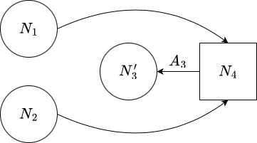
Figure 11: The quiver diagram obtained by deleting the arrows $3\rightarrow 1,\,3\rightarrow 2$ from Figure 10.

Let $(\tilde{V}_{1},G_{1},\theta_{1})$ be the input data of the quiver where $\tilde{V}_{1}=\mathbb{C}^{N_{1}\times N_{4}}\oplus\mathbb{C}^{N_{2}\times N_{4}}\oplus\mathbb{C}^{N_{4}\times N_{3}^{\prime}}$, and $G_{1},\,\theta_{1}$ be as above. Let $\mathcal{X}_{1}:=\tilde{V}_{1}\sslash_{\theta_{1}}G_{1}$ be the quiver variety of the quiver diagram in Figure 11. The affine variety $Z_{1}$ can be viewed as a complete intersection in the affine variety $\tilde{V}_{1}$ defined by $B_{1}A_{3}=0,\,B_{2}A_{3}=0$. The GIT quotient $\mathcal{Z}_{1}:=Z_{1}\sslash_{\theta_{1}}G_{1}$ is a subvariety in $\mathcal{X}_{1}$ defined by equations

$$B_{1}A_{3}=0,\,B_{2}A_{3}=0\,.$$ (2.20)

Example 2.11.

We perform another quiver mutation $\mu_{1}$ to the quiver diagram in Figure 10 and get the quiver diagram below.

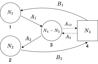
Figure 12: The quiver diagram obtained by applying $\mu_{1}\mu_{3}$ to the original $D_{3}$ quiver. Notice that the integer assigned to node 1 is $N_{4}-N_{1}=N_{2}$. The dashed opposite arrows are annihilated.

To construct the new potential, we first replace the factor $A_{1}B_{1}$ by the matrix $A_{12}$ and add a new cubic term $tr(B_{1}A_{1}A_{12})$ arising from the 3-cycle $4\rightarrow 1\rightarrow 3\rightarrow 4$, and we get a new potential $W_{2}^{\prime}=tr(A_{12}A_{3})+tr(A_{2}B_{2}A_{3})+tr(B_{1}A_{1}A_{12})$. In $W_{2}^{\prime}$, there is a quadratic term $tr(A_{12}A_{3})$, so we take the derivative to $W^{\prime}$ in terms of these two factors

$$d_{A_{12}^{ab}}W_{2}^{\prime}=0,\,\,d_{A_{3}^{ab}}W_{2}^{\prime}=0\,,$$ (2.21)

and get constraints for $W_{2}^{\prime}$,

$$A_{3}+A_{2}B_{2}=0,\,\,A_{12}+A_{2}B_{2}=0\,.$$ (2.22)

Substituting $A_{3}=-A_{2}B_{2}$ and $A_{12}=-A_{2}B_{2}$, we derive the correct potential $W_{2}=tr(B_{1}A_{1}A_{2}B_{2})$, where we have neglect the negative sign in front of it.

Let $(V_{2},G_{2},\theta_{2})$ be the input data for the quiver variety of Figure 12, with $V_{2}=\mathbb{C}^{N_{4}\times N_{2}}\oplus\mathbb{C}^{N_{2}\times N_{3}^{\prime}}\oplus\mathbb{C}^{N_{3}^{\prime}\times N_{2}}\oplus\mathbb{C}^{N_{2}\times N_{4}}$, $G_{2}=GL(N_{2})\times GL(N_{2})\times GL(N_{3}^{\prime})$, and a character $\theta_{2}(g)=\prod_{i=1}^{3}\det(g_{i})^{\sigma_{i}}$ with

$$\sigma_{1}<0,\,\,\sigma_{2}>0,\,\,\sigma_{3}<0\,.$$ (2.23)

The semistable locus is

$$V^{ss}_{2}(G_{2})=\{B_{1},A_{1},B_{2}\text{ nondegenerate}\}\,.$$ (2.24)

Consider the critical locus $Z_{2}=Z(dW_{2})$ of the potential $W_{2}$. It is equivalent to the following equations,

$$B_{1}A_{1}A_{2}=0,\,A_{1}A_{2}B_{2}=0,\,B_{2}B_{1}A_{1}=0,\,A_{2}B_{2}B_{1}=0\,.$$ (2.25)

The non-degeneracy of $B_{1},\,A_{1}$ and the equation $B_{1}A_{1}A_{2}=0$ imply that $A_{2}=0$. Therefore, relations (2.25) can be reduced to

$$A_{2}=0,\,B_{2}B_{1}A_{1}=0.$$ (2.26)

Consider a new quiver diagram below,

Figure 13: A quiver diagram obtained by deleting the arrow $3\rightarrow 2$ from Figure 12.

Denote the corresponding input data of the quiver by $(\tilde{V}_{2},G_{2},\theta_{2})$, and denote its quiver variety by $\mathcal{X}_{2}:=\tilde{V}_{2}\sslash_{\theta_{2}}G_{2}$. We find that $Z(dW_{2})$ can be viewed as an affine subvariety of $\tilde{V}_{2}$ defined by $B_{2}B_{1}A_{1}=0$. Therefore, the variety we are seeking for $\mathcal{Z}_{2}=\{B_{2}B_{1}A_{1}=0\}\sslash_{\theta_{2}}G_{2}$ is a subvariety in the quiver variety $\mathcal{X}_{2}$.

Example 2.12.

Applying $\mu_{2}$ to the quiver diagram in Figure 12, we obtain the following quiver diagram.

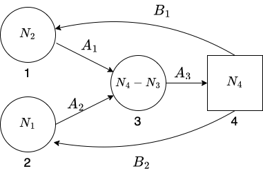
Figure 14: Quiver diagram by performing $\mu_{2}\mu_{1}\mu_{3}$ to the original $D_{3}$-quiver. The integer assigned to node 2 is $N_{4}-N_{2}=N_{1}$

The potential is obtained by replacing $A_{2}B_{2}$ by $A_{3}$ and adding the cubic term $tr(B_{2}A_{2}A_{3})$, so $W_{3}=tr(B_{1}A_{1}A_{3})+tr(B_{2}A_{2}A_{3})$. Denote the input data for the quiver variety by $(V_{3},G_{3},\theta_{3})$ where $V_{3}=\mathbb{C}^{N_{2}\times N_{3}^{\prime}}\oplus\mathbb{C}^{N_{1}\times N_{3}^{\prime}}\oplus\mathbb{C}^{N_{3}^{\prime}\times N_{4}}\oplus\mathbb{C}^{N_{4}\times N_{2}}\oplus\mathbb{C}^{N_{4}\times N_{1}}$, $G_{3}=GL(N_{2})\times GL(N_{3}^{\prime})\times GL(N_{1})$. We choose the character of $G_{3}$ as

$$\theta_{3}(g)=\det(g_{1})^{\sigma_{1}}\det(g_{2})^{\sigma_{2}}\det(g_{3})^{\sigma_{3}},\,\,\sigma_{1}<0,\,\,\sigma_{2}<0,\,\,\sigma_{3}>0\,.$$ (2.27)

An element in the semistable locus $V^{ss}_{\theta_{3}}(G_{3})$ must satisfy the condition that $B_{1},B_{2}$ and $A_{3}$ are nondegenerate. Consider the critical locus $Z_{3}=Z(dW_{3})$. It is equivalent to the following equations

$$A_{1}A_{3}=0,\,A_{2}A_{3}=0,\,B_{1}A_{1}+B_{2}A_{2}=0,\,A_{3}B_{1}=0,\,A_{3}B_{2}=0.$$ (2.28)

The non-degeneracy of $A_{3}$ implies that $A_{1}=0,\,A_{2}=0$, so we have

$$Z_{3}^{ss}(G_{3})=\{A_{1}=0,\,A_{2}=0,\,A_{3},\,B_{1},\,B_{2},\,A_{3}\,\text{ non-degenerate }\,A_{3}B_{1}=0,\,A_{3}B_{2}=0\}\,.$$ (2.29)

Consider another quiver obtained from that in Figure 14 by deleting arrows $1\rightarrow 3$ and $2\rightarrow 3$,

Let $(\tilde{V}_{3},G_{3},\theta_{3})$ be the input date of the new quiver, and $\mathcal{X}_{3}$ be the quiver variety. We can view $Z_{3}$ as a complete intersection $\{A_{3}B_{1}=0,\,A_{3}B_{2}=0\}$ in $\tilde{V}_{3}$. Then $\mathcal{Z}_{3}=\{A_{3}B_{1}=0,\,A_{3}B_{2}=0\}\sslash_{\theta_{3}}G_{3}$ can be viewed as a subvariety in $\mathcal{X}_{3}$. The variety $\mathcal{Z}_{3}$ is the one under consideration. We notice that the variety $\mathcal{Z}_{3}$ is naturally isomorphic to the variety $\mathcal{Z}_{1}$.

Until now, we have performed quiver mutations $\mu_{3},\mu_{1},\mu_{2}$ to the original $D_{3}$ quiver. Readers may pause here, perform quiver mutations $\mu_{3}$, $\mu_{1}$, $\mu_{2}$ consecutively again, and construct the corresponding quiver varieties. The following quivers are very simple since their potentials are all trivial. We will just list them all for readers to check their answers.

Example 2.13.

We perform quiver mutations $\mu_{3}\rightarrow\mu_{1}\rightarrow\mu_{2}\rightarrow\mu_{3}\rightarrow\mu_{1}\rightarrow\mu_{2}$ and obtain the following quiver diagrams where we mark the mutation relations.

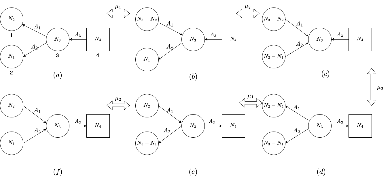
Figure 15: The quiver diagrams obtained by quiver mutations.

In order to construct the corresponding quiver varieties, we only need to fix the phases of those gauge groups, which are listed in the following table.

Figure	character	Phase
(a)	$\theta_{4}$	$\sigma_{1}<0,\,\sigma_{2}<0,\,\sigma_{3}<0$
$(b)$	$\theta_{5}$	$\sigma_{1}>0,\,\sigma_{2}<0,\,\sigma_{3}<0,\,(N_{3}-N_{2})\sigma_{1}+\sigma_{3}<0$
$(c)$	$\theta_{6}$	$\sigma_{1}>0,\,\sigma_{2}>0,\,\sigma_{3}<0,\,(N_{3}-N_{2})\sigma_{1}+(N_{3}-N_{1})\sigma_{2}+\sigma_{3}<0$
$(d)$	$\theta_{7}$	$\sigma_{1}<0,\,\sigma_{2}<0,\,\sigma_{3}>0,\,(N_{3}-N_{2})\sigma_{1}+(N_{3}-N_{1})\sigma_{2}+\sigma_{3}>0$
$(e)$	$\theta_{8}$	$\sigma_{1}>0,\,\sigma_{2}<0,\,\sigma_{3}>0,\,(N_{3}-N_{1})\sigma_{2}+\sigma_{3}>0$
$(f)$	$\theta_{9}$	$\sigma_{1}>0,\,\sigma_{2}>0,\,\sigma_{3}>0$

Table 2: Phases of the quivers in Figure 15.

One can check that for each quiver diagram and its associated input data for the quiver variety $(V_{i},G_{i},\theta_{i})$, the semistable locus is $V_{i}^{ss}(G_{i})=\{A_{1},A_{2},A_{3}\text{ non-degenerate}\}$. We denote the corresponding quiver varieties by $\mathcal{X}_{i}=V_{i}\sslash_{\theta_{i}}G_{i}$, $i=4,5,6,7,8,9$.

3 Gromov-Witten invariants and wall-crossing theorem

We will introduce the GW theory and the wall-crossing theorem. Readers who are familiar with related materials can skip this section.

3.1 Gromov-Witten invariants

We refer to the beautiful book [CK99] about the fundamental properties of GW theory.

Definition 3.1.

Let $\mathcal{X}$ be a smooth projective variety. A stable map to $\mathcal{X}$ denoted by $(C,p_{1},\ldots,p_{n};f)$ consists of the following data:

1. a nodal curve $(C,p_{1},\ldots,p_{n})$ with $n\geq 0$ distinct nonsingular markings,

2. a stable map $f:(C,p_{1},\ldots,p_{n})\rightarrow\mathcal{X}$ such that every component of $C$ of genus 0, which is contracted by $f$, must have at least three special (marked or singular) points, and every component of $C$ of genus one which is contracted by $f$, must have at least one special point.

The class or the degree of a stable map $(C,p_{1},\ldots,p_{n};f)$ is defined as the homology class of the image $\beta=f_{*}[C]$. For a fixed curve class $\beta\in H_{2}(\mathcal{X},\mathbb{Z})$, let $\overline{M}_{g,n}(\mathcal{X},\beta)$ denote the stack of stable maps from $n$-marked and genus-g curves $C$ to $\mathcal{X}$ such that $f_{*}[C]=\beta$. When $\mathcal{X}$ is projective, $\overline{M}_{g,n}(\mathcal{X},\beta)$ is a proper separated DM stack and admits a perfect obstruction theory. Hence we can construct the virtual fundamental class $[\overline{M}_{g,n}(\mathcal{X},\beta)]^{vir}\in A_{\text{vdim}}(\overline{M}_{g,n}(\mathcal{X},\beta))$ where $\text{vdim}=\int_{\beta}c_{1}(X)+(\dim(\mathcal{X})-3)(1-g)+n$. See [LT98, BF97, Beh97].

Let $\pi:\mathcal{C}_{g,n}\rightarrow\overline{M}_{g,n}(\mathcal{X},\beta)\,,$ be the universal curve and $s_{i}$ are sections of $\pi$ for each marking $p_{i}$. Let $\omega_{\pi}$ be the relative dualizing sheaf and $\mathcal{P}_{i}=s_{i}^{*}(\omega_{\pi})$ be the cotangent bundle at the $i$-th marking. Define the $\psi$-class by $\psi_{i}:=c_{1}(\mathcal{P}_{i})\in H^{2}(\overline{M}_{g,n}(\mathcal{X},\beta))$. Define evaluation maps by

$$ev_{i}:\overline{M}_{g,n}(\mathcal{X},\beta) \longmapsto\mathcal{X}$$

$$(C,p_{1},\ldots,p_{n};f) \longmapsto f(p_{i})\,.$$ (3.1)

Let $\gamma_{1},\ldots,\gamma_{n}\in H^{*}(\mathcal{X})$ be cohomology classes and $a_{i}$ $i=1,\ldots,n$ be positive integers. The GW invariant is defined as

$$\langle\tau_{a_{1}}\gamma_{1},\ldots,\tau_{a_{n}}\gamma_{n}\rangle_{g,n,\beta}:=\int_{[\overline{M}_{g,n}(\mathcal{X},\beta)]^{vir}}\prod_{i=1}^{n}\psi_{i}^{a_{i}}ev_{i}^{*}(\gamma_{i})\,.$$ (3.2)

Let $\alpha_{0}=1,\alpha_{1},\ldots,\alpha_{m}\in H^{*}(\mathcal{X})$ be a set of generators of cohomology group, and $\alpha^{0},\alpha^{1},\ldots,\alpha^{m}\in H^{*}(\mathcal{X})$ be the Poincaré dual. The small $\mathcal{J}$-function of $\mathcal{X}$, which comprises genus-zero GW invariants, is defined by

$$\mathcal{J}^{\mathcal{X}}(Q,\mathbf{t},u)=\sum_{i=0}^{m}\sum_{(k\geq 0,\beta)}\alpha^{i}\langle\frac{\alpha_{i}}{u(u-\psi_{\bullet})}\mathbf{t}\ldots\mathbf{t}\rangle_{0,k+1,\beta}\frac{Q^{\beta}}{k!}\,.$$ (3.3)

where $\mathbf{t}\in H^{\leq 2}(\mathcal{X})$.

When $\mathcal{X}$ admits a torus action, denoted by $S$, then $S$ induces an action on $\overline{M}_{g,n}(\mathcal{X},\beta)$ by sending a stable map $(C,p_{1},\ldots,p_{n};\,f)$ to $(C,p_{1},\ldots,p_{n};\,s\circ f)$ for each $s\in S$. Let $F$ denote a torus fixed locus of $\overline{M}_{g,n}(\mathcal{X},\beta)$. There is an induced equivariant perfect obstruction theory on $\overline{M}_{g,n}(\mathcal{X},\beta)$, hence the equivariant virtual fundamental class. Let $H^{*}_{S}(\mathcal{X}):=H^{*}(\mathcal{X}\times_{G}EG)$ be equivariant cohomology group of $\mathcal{X}$. For $\omega_{i}\in H^{*}_{S}(\mathcal{X})$, the equivariant GW invariants are defined via the virtual localization theorem as follows,

$$\langle\tau_{a_{1}}\omega_{1},\ldots,\tau_{a_{n}}\omega_{n}\rangle_{g,n,\beta}^{S}:=\sum_{F}\int_{F}\frac{i_{F}^{*}\left(\prod_{i=1}^{n}\psi_{i}^{a_{i}}ev_{i}^{*}(\omega_{i})\right)}{e^{S}(N^{vir}_{F})}\,.$$ (3.4)

The summation is over all torus fixed locus $F$, the map $i_{F}:F\rightarrow\overline{M}_{g,n}(\mathcal{X},\beta)$ is the embedding, and $N_{F}^{vir}$ is the virtual normal bundle of $F$. Suppose $\mathcal{X}$ is projective and $\gamma_{i}^{\prime}s$ are the non-equivariant limit of $\omega_{i}^{\prime}s$ via the map $H^{*}_{S}(\mathcal{X})\rightarrow H^{*}(\mathcal{X})$, and then the nonequivariant limit of $\langle\tau_{d_{1}}\omega_{1},\ldots,\tau_{d_{n}}\omega_{n}\rangle_{g,n,\beta}^{S}$ is equal to the regular GW invariant $\langle\tau_{d_{1}}\gamma_{1},\ldots,\tau_{d_{n}}\gamma_{n}\rangle_{g,n,\beta}$. See [GP99].

Similarly, we can define the equivariant small $\mathcal{J}$-function of $\mathcal{X}$ by changing each correlator in (3.3) to the equivariant version. We denote the equivariant small $\mathcal{J}$ function by $\mathcal{J}^{\mathcal{X},S}(Q,\mathbf{t},u)$.

3.2 Genus-zero wall-crossing theorem

In this subsection, we introduce the genus-zero wall-crossing theorem in the context of Cheong, Ciocan-Fontanine, Kim, and Maulik [CFKM14, CCFK15, CFK14, CFK16]. We only involve necessary parts for our purpose.

Fix a valid input data for a GIT quotient $(V,G,\theta)$, and denote the corresponding GIT quotient by $\mathcal{X}:=V\sslash_{\theta}G$.

Definition 3.2.

A quasimap from $\mathbb{P}^{1}$ to $V\sslash_{\theta}G$ consists of the data $(P,\sigma)$ where

• $P$ is a principle $G$-bundle on $\mathbb{P}^{1}$,

• $\sigma$ is a section of the induced bundle $P\times_{G}V$ with the fiber $V$ on $\mathbb{P}^{1}$.

The class of a quasimap is defined as $\beta\in\operatorname{Hom}(\operatorname{Pic}^{G}(V),\mathbb{Z})$, such that for each line bundle $L\in\operatorname{Pic}^{G}(V)$,

$$\beta(L)=\deg_{\mathbb{P}^{1}}(\sigma^{*}(P\times_{G}L))\,.$$ (3.5)

Definition 3.3.

An element $\beta\in\operatorname{Hom}(\operatorname{Pic}^{G}(V),\mathbb{Z})$ is called an $I$-effective class if it is the class of a quasimap from $\mathbb{P}^{1}$ to $V\sslash_{\theta}G$. Denoted the semigroup of $I$-effective classes by $\operatorname{Eff}(V,G,\theta)$.

Definition 3.4.

A quasimap $(P,\sigma)$ from $\mathbb{P}^{1}$ to $V\sslash_{\theta}G$ is stable if

1. the set $B:=\sigma^{-1}(V^{us})\subset\mathbb{P}^{1}$ is finite, and points in $B$ are called base points of the quasimap,

2. $\mathbf{L}_{\theta}:=\sigma^{*}(P\times_{G}L_{\theta})$ is ample, where $L_{\theta}=V\times\mathbb{C}_{\theta}$.

Denote the moduli stack of all stable qusimaps from $\mathbb{P}^{1}$ to $V\sslash_{\theta}G$ of class $\beta$ as $QG_{\beta}(V\sslash G)$. This moduli stack is the so-called stable quasimap graph space in [CFKM14].

Theorem 3.5 ([CFKM14]).

The stack $QG_{\beta}(V\sslash_{\theta}G)$ is a separated Deligne-Mumford stack of finite type, proper over the affine quotient $Spec(H^{0}(V,\mathcal{O}_{V})^{G})$. It admits a canonical perfect obstruction theory if $V$ has at most lci singularities.

Let $[\zeta_{0},\zeta_{1}]$ be homogeneous coordinates on $\mathbb{P}^{1}$, and it has a standard $\mathbb{C}^{*}$ action given by

$$t[\zeta_{0},\zeta_{1}]=[t\zeta_{0},\zeta_{1}],t\in\mathbb{C}^{*}\,.$$ (3.6)

The $\mathbb{C}^{*}$-action on $\mathbb{P}^{1}$ induces an action on $QG_{\beta}(V\sslash_{\theta}G)$. If a quasimap $(P,\sigma)\in QG_{\beta}(V\sslash_{\theta}G)$ is $\mathbb{C}^{*}$-fixed, then all base points and the entire degree $\beta$ must be supported over the torus fixed points $[0:1]$ or $[1:0]$.

Consider the $\mathbb{C}^{*}$-fixed locus $F_{\beta}$ where everything is supported over the point $[0:1]\in\mathbb{P}^{1}$ and the map $ev_{\bullet}:\mathbb{P}^{1}\backslash\{[0:1]\}\rightarrow V\sslash_{\theta}G$ is constant.

Definition 3.6.

Define the quasimap small $I$-function of a projective GIT quotient $V\sslash_{\theta}G$ as

$$I^{V\sslash_{\theta}G}(q,u)=1+\sum_{\beta\neq 0}q^{\beta}I_{\beta}^{V\sslash_{\theta}G}(u)\,\,,I_{\beta}^{V\sslash_{\theta}G}(u)=(ev_{\bullet})_{*}\left(\frac{[F_{\beta}]^{vir}}{e^{\mathbb{C}^{*}}(N_{F_{\beta}}^{vir})}\right)\,,$$ (3.7)

where the sum is over all $I$-effective classes of $(V,G,\theta)$.

Assume $V\sslash_{\theta}G$ is projective, and $V$ admits a torus action ${S}$ which commutes with the action of $G$ on $V$. Hence the $S$ acts on $V\sslash_{\theta}G$. The torus action is good if the torus fixed locus $(V\sslash_{\theta}G)^{S}$ is a finite set. There is an induced action of $S$ on $QG_{\beta}(V\sslash_{\theta}G)$ by sending $(P,u)\in QG_{\beta}(V\sslash_{\theta}G)$ to $s\circ u$ for each $s\in S$. Moreover, the perfect obstruction theory is canonical $S$-equivariant [CFKM14]. The same formula defines the equivariant quasimap small $I$-function of $V\sslash_{\theta}G$ as Definition 3.6 with all characteristic classes and pushforwards replaced by the equivariant version. We denote the equivariant quasimap small $I$-function of $V\sslash_{\theta}G$ by $I^{V\sslash_{\theta}G,S}(q,z)$.

Theorem 3.7 ([CFK14]).

Assume $V\sslash_{\theta}G$ is a (quasi-)projective variety with a good torus action, and $V$ admits at most lci singularities. Then the following (equivariant) wall-crossing formula holds when $(V,G,\theta)$ is semi-positive,

$$\mathcal{J}^{V\sslash_{\theta}G,S}(q,\mathbf{t},u)=\frac{I^{V\sslash_{\theta}G,S}(q,u)}{I_{0}(q)}\,,$$ (3.8)

via mirror map,

$$\mathbf{t}=\frac{I_{1}(q)}{I_{0}(q)}\in H^{\leq 2}(V\sslash G)\,,$$ (3.9)

where the $I_{0}(q)$, $I_{1}(q)$ are defined as coefficients of $1$ and $u^{-1}$ in the following expansion,

$$I^{V\sslash_{\theta}G,S}(q,u)=I_{0}(q)+\frac{I_{1}}{u}(q)+O(\frac{1}{u^{2}})\,.$$ (3.10)

Furthermore when $V\sslash_{\theta}G$ is Fano of index at least 2, $I_{0}(q)=1$ and $\mathbf{t}=0$. Hence in this situation

$$\mathcal{J}^{V\sslash_{\theta}G,S}(q,u)=I^{V\sslash_{\theta}G,S}(q,u)\,.$$ (3.11)

4 Equivariant quasimap small $I$-functions

4.1 Abelian/nonabelian correspondence for $I$-functions

We will mainly follow the work of Rachel Webb about the abelian-nonabelian correspondence to display the quasimap $I$-functions of our examples, see [Web18, Web21].

Fix a valid input $(V,G,\theta)$ for a GIT quotient $V\sslash_{\theta}G$, and we assume that $V$ has at most lci singularities. Let $T=(\mathbb{C}^{*})^{r}\subseteq G$ denote the maximal torus of $G$ and let $W_{T}=N_{T}/T$ denote the Weyl group. We will use a letter $w$ to represent a general element in the Weyl group $W_{T}$ and its representative in $N_{T}$ with abuse of notation. Notice that any character $\theta$ of $G$ is also a character of $T$ by the inclusion $\chi(G)\subseteq\chi(T)$. We denote the semistable, stable and unstable locus of $V$ under the action of $T$ in character $\theta$ by $V^{ss}_{\theta}(T)$, $V^{s}_{\theta}(T)$, and $V^{us}_{\theta}(T)$. We may instead use notations $V^{ss}(T)$, $V^{s}(T)$, and $V^{us}(T)$ when there is no confusion for the character. Assume that $V^{ss}(T)=V^{s}(T)$ and $T$ acts freely on $V^{ss}(T)$, so that we obtain a smooth variety $V\sslash_{\theta}T:=V^{s}(T)/T$. Assume that a torus $S$ acts on $V$ and commutes with the action of G. Hence $S$ acts on $V\sslash_{\theta}G$ and $V\sslash_{\theta}T$. Assume that the torus action $S$ on $V\sslash_{\theta}G$ and $V\sslash_{\theta}T$ is good.

The relation between $H^{*}(V\sslash_{\theta}G)$ and $H^{*}(V\sslash_{\theta}T)$ is studied by [ESm89, Mar00, Kir05]. The map $V\sslash_{\theta}G\dashrightarrow V\sslash_{\theta}T$ is realized as follows

(4.1)

The Weyl group $W$ acts on $V^{s}(G)/T$, and therefore on $H^{*}(V^{s}(G)/T)$. The above diagram induces the following classical identification for the cohomology groups

$$H_{S}^{*}(V\sslash_{\theta}G,\mathbb{Q})\cong H_{S}^{*}(V^{s}(G)/T,\mathbb{Q})^{W}\,.$$ (4.2)

See [Web18, Proposition 2.4.1] for proof for the chow groups version. For each $\gamma\in H_{S}^{*}(V\sslash_{\theta}G,\mathbb{Q})$, we say $\tilde{\gamma}\in H_{S}^{*}(V\sslash_{\theta}T,\mathbb{Q})^{W}$ is a lifting of $\gamma$ if $a^{*}(\tilde{\gamma})=p^{*}(\gamma)$. Such lifting is usually not unique. For each $\eta\in\chi(G)\subset\chi(T)$, there are line bundles $V\times\mathbb{C}_{\eta}\in\operatorname{Pic}^{G}(V)$ and $V\times\mathbb{C}_{\eta}\in\operatorname{Pic}^{T}(V)$. Also, there is a natural map from $\operatorname{Pic}^{G}(V)$ to $\operatorname{Pic}^{T}(V)$ by restriction. Therefore we have the following commutative diagram

(4.3)

Taking $\operatorname{Hom}(-,\mathbb{Z})$ to the above diagram, we get the following commutative diagram,

(4.4)

For any $\xi\in\chi(T)$, denote by $\mathcal{L}_{\xi}:=V^{s}(T)\times_{T}\mathbb{C}_{\xi}$ the line bundle over $V\sslash_{\theta}T$. For any $\tilde{\beta}\in\operatorname{Hom}(\operatorname{Pic}^{T}(V),\mathbb{Z})$, denote by $\tilde{\beta}(\xi):=\tilde{\beta}(c_{1}(\mathcal{L}_{\xi}))$, and it also equals $v_{1}(\tilde{\beta})(\xi)$ by the above diagram.

Lemma 4.1.

([CFKM14]) When $r_{1}$ restricts to $I$-effective classes $\operatorname{Eff}(V,T,\theta)\subseteq\operatorname{Hom}(\operatorname{Pic}^{T}(V),\mathbb{Z})$ in the source and $\operatorname{Eff}(V,G,\theta)\subseteq\operatorname{Hom}(\operatorname{Pic}^{G}(V),\mathbb{Z})$ in the target, it has finite fibers.

Theorem 4.2 ([Web18]).

The equivariant quasimap small $I$-functions of $V\sslash_{\theta}G$ and $V\sslash_{\theta}T$ satisfy

$$p^{*}I_{\beta}^{V\sslash_{\theta}G,S}(u)=a^{*}\left[\sum_{\tilde{\beta}\rightarrow\beta}\prod_{\rho}\frac{\prod_{k\leq\tilde{\beta}(\rho)}(c_{1}(\mathcal{L}_{\rho})+ku)}{\prod_{k\leq 0}(c_{1}(\mathcal{L}_{\rho})+ku)}I_{\tilde{\beta}}^{V\sslash_{\theta}T,S}(u)\right]$$ (4.5)

where the sum is over all preimages $\tilde{\beta}$ of $\beta$ under the map $r_{1}$ in above diagram (4.4) and the product is over all roots $\rho$ of $G$.

Since the map $p$ is surjective, $p^{*}$ is injective, then $I^{V\sslash_{\theta}G}$ is uniquely determined by $p^{*}I^{V\sslash_{\theta}G}$. In the following, we will make no difference between $I_{\beta}^{V\sslash_{\theta}G,S}$ and $p^{*}I_{\beta}^{V\sslash_{\theta}G,S}$.

Consider a $G$-equivariant bundle $E$ over $V$, and assume $s$ is a $G$-equivariant regular section of the bundle $E\times V\rightarrow V$. Let $Z:=Z(s)\subseteq V$ be the zero loci of $s$. Taking $Z$ into consideration, we can extend the diagram (4.1) to

(4.6)

and extend the diagram (4.4) to

(4.7)

For each $\xi\in\chi(T)$, and $\beta\in\operatorname{Home}(\operatorname{Pic}^{T}(V),\mathbb{Z})$, denote

$$C(\beta,\xi):=\frac{\prod_{k\leq 0}(c_{1}(\mathcal{L}_{\xi})+ku)}{\prod_{k\leq\beta(\xi)}(c_{1}(\mathcal{L}_{\xi})+ku)}\,.$$ (4.8)

Assume that the torus $S$ acts on $Z$ and is good. The equivariant quasimap small $I$-functions of $Z\sslash_{\theta}G$ and $V\sslash_{\theta}T$ satisfy the following relation, which can be viewed as an abelian/nonabelian quantum Lefschetz theorem.

Theorem 4.3 ([Web18, Web21]).

Assume that weights of $E$ with respect to the action of $T$ are $\epsilon_{j}$, for $j=1,\ldots,m$, and $\rho_{i}$ for $i=1,\ldots,r$ are roots of $G$. Then for a fixed $\delta\in\operatorname{Hom}(\operatorname{Pic}^{G}(V),\mathbb{Q})$, we have the following relation between $I$-functions of $Z\sslash_{\theta}G$ and $V\sslash_{\theta}T$,

$$\sum_{\beta\rightarrow\delta}\phi^{*}I_{\beta}^{Z\sslash_{\theta}G,S}(u)=\sum_{\tilde{\delta}\rightarrow\delta}\left(\prod_{i=1}^{m}C(\tilde{\delta},\epsilon_{i})^{-1}\right)\left(\prod_{i=1}^{r}C(\tilde{\delta},\rho_{i})^{-1}\right)b^{*}a^{*}I_{\tilde{\delta}}^{V\sslash T,S}(u)$$ (4.9)

where $\tilde{\delta}\in\operatorname{Hom}(\operatorname{Pic}^{T}(V),\mathbb{Q})$ are preimages of $\delta$ via $r_{1}$, and $\beta\in\operatorname{Hom}(\operatorname{Pic}^{G}(Z),\mathbb{Q})$.

4.2 Quasimap small $I$-functions of our examples

We will apply the abelian/nonabelian correspondence for $I$-functions to find the equivariant quasimap small $I$-functions for the varieties displayed in Section 2.

Conventions and Notations

• Denote $[N]:=\{1,2,\ldots,N\}$.

• Fix a quiver diagram $(Q_{f}\subset Q_{0},Q_{1},W)$ with an assigned integer vector $\vec{v}=(N_{i})_{i\in Q_{0}}$. Let $T=\prod_{i\in Q_{0}\backslash Q_{f}}(\mathbb{C}^{*})^{N_{i}}\subset G$ be the maximal torus in the non-abelian group $G$. Consider a line bundle $V\times\mathbb{C}$ over $V$, and $t=(t_{I}^{i})_{i\in Q_{0}\backslash Q_{f},\,I\in[N_{i}]}\in T$ acts on it by $t\cdot((A_{i\rightarrow j}),v)=(g(A_{i\rightarrow j}),t^{i}_{I}v)$. This action defines a line bundle $L_{I}^{i}:=V^{ss}(T)\times_{T}\mathbb{C}\rightarrow V^{ss}(T)/T$. Define $x^{i}_{I}:=c_{1}(L_{I}^{i})\in H^{*}(V\sslash_{\theta}T)$ to be the first chern class of such bundle for each $i\in Q_{0}\backslash Q_{f},I\in[N_{i}]$.

• Let $S=(\mathbb{C}^{*})^{N_{8}+N_{9}}$ and $S^{1}=(\mathbb{C}^{*})^{N_{4}}$. We already know that $S$ acts on the star-shaped quiver and its quiver mutation, and $S^{1}$ acts on $D_{3}$ and its quiver mutations. Denote the equivariant cohomology ring of a point under a trivial action of $S$ by $H^{*}_{S}(pt,\mathbb{Q})=Q[\lambda_{1},\ldots,\lambda_{N_{8}},\lambda_{N_{8}+1},\ldots,\lambda_{N_{8}+N_{9}}]$ and that of $S^{1}$ by $H^{*}_{S^{1}}(pt,\mathbb{Q})=Q[\lambda_{1},\ldots,\lambda_{N_{4}}]$.

• For each variety, let $\vec{q}=(q_{i})_{i\in Q_{0}\backslash Q_{f}}$ denote the kähler parameters by abuse of notation except when we need to consider the transformation between their kähler parameters under a quiver mutation.

• Denote by $\operatorname{Eff}^{s}:=\operatorname{Eff}(V_{s},G_{s},\theta_{s})$ the semigroup of $I$-effective classes of the general star-shaped quiver variety, and $\operatorname{Eff}^{ms}:=\operatorname{Eff}(\tilde{V}_{s},\tilde{G}_{s},\tilde{\theta}_{s})$ the semigroup of $I$-effective classes of the variety $\widetilde{\mathcal{X}}_{s}$ in Exmaple 2.9. Denote by $\operatorname{Eff}^{s}_{T}$ and $\operatorname{Eff}^{ms}_{T}$ their lifting to $\operatorname{Hom}(\operatorname{Pic}^{T}(V_{s}),\mathbb{Q})$ and $\operatorname{Hom}(\operatorname{Pic}^{T}(\overline{V}_{s}),\mathbb{Q})$. Denote by $\operatorname{Eff}^{i}$ the semigroups of $I$-effective classes of quiver varieties $\mathcal{X}_{i}$ considered in Section 2, and by $\operatorname{Eff}^{i}_{T}$ their lifting via $r_{1}$.

For a general quiver diagram $(Q_{f}\subset Q_{0},Q_{1},W)$ with assigned integer vector $\vec{v}=(N_{i})$, let $(V,G,\theta)$ be the input data of the quiver variety $V\sslash_{\theta}G$. A stable quasimap $(P,\sigma)$ from $\mathbb{P}^{1}$ to $\mathcal{X}=V\sslash_{\theta}G$ is equivalent to the following ingredients:

1. a vector bundle of matrices $P$ which can be written as $\oplus_{i\rightarrow j\in Q_{1}}\oplus_{I=1}^{N_{i}}\oplus_{J=1}^{N_{j}}\mathcal{O}(n^{i}_{I}-n^{j}_{J})$,

2. a section $\sigma$ of the above bundle which maps all but finite points of $\mathbb{P}^{1}$ to semi-stable locus.

By our examples in Section 2, a semistable point $(A_{i\rightarrow j})_{i\rightarrow j\in Q_{1}}$ in $V$ is described by the non-degeneracy of some matrices. If some matrix $A_{i\rightarrow j}$ is non-degenerate in $V^{ss}(G)$, the corresponding factor $\oplus_{I=1}^{N_{i}}\oplus_{J=1}^{N_{j}}\mathcal{O}(n^{i}_{I}-n^{j}_{J})$ in the vector bundle $P$ must admit a section that are non-degenerate on all $\mathbb{P}^{1}$ except for finite many points. Hence, such vectors $\vec{n}^{i}=(n^{i}_{I})_{I=1}^{N_{i}},\vec{n}^{j}=(n^{j}_{J})_{J=1}^{N_{j}}$ satisfy the following conditions:

• for the $N_{i}\times N_{j}$ matrix $(n^{i}_{I}-n^{j}_{J})_{I=1,J=1}^{N_{i},N_{j}}$, in each row and each column, there is at least one entry $(I,J)$ such that $n^{i}_{I}-n^{j}_{J}\geq 0$,

• the new $N_{i}\times N_{j}$ matrix $(\max\{n^{i}_{I}-n^{j}_{J},0\})_{I=1,J=1}^{N_{i},N_{j}}$ is row or column full-rank.

Those vectors $(n^{i}_{I})_{i\in Q_{0}\backslash Q_{f},I=1,\ldots,N_{i}}$ actually are the preimages of of $\operatorname{Eff}(V,G,\theta)$ in the diagram (4.4) under $r_{1}$ and Lemma 4.1, denoted by $\operatorname{Eff}_{T}$, which explicitly are $\operatorname{Eff}^{s}_{T}$, $\operatorname{Eff}^{ms}_{T}$ and $\operatorname{Eff}^{i}_{T}$ for our examples. The map $r_{1}$ sends $(n^{i}_{I})_{i,I}$ to $(\lvert\vec{n}^{i}\rvert)_{i\in Q_{0}\backslash Q_{f}}$.

Lemma 4.4.

For a quiver variety $\mathcal{X}=V\sslash_{\theta}G$ with a torus $S$ action which comes from frame nodes, its equivariant quasimap small $I$-function is

$$p^{*}I^{\mathcal{X},S}(\vec{q},u) =\sum_{(\vec{n}^{i})\in\operatorname{Eff}_{T}}\prod_{i\in Q_{0}\backslash Q_{f}}\prod_{\begin{subarray}{c}I,J=1\\ I\neq J\end{subarray}}^{N_{i}}a^{*}\Big{(}\frac{\prod_{l\leq n^{i}_{I}-n^{i}_{J}}(x^{i}_{I}-x^{i}_{J}+lu)}{\prod_{l\leq 0}(x^{i}_{I}-x^{i}_{J}+lu)}$$

$$\prod_{i\rightarrow j\in Q_{1}}\prod_{I=1}^{N_{i}}\prod_{J=1}^{N_{j}}\frac{\prod_{l\leq 0}(x^{i}_{I}-x^{j}_{J}+lu)}{\prod_{l\leq n^{i}_{I}-n^{j}_{J}}(x^{i}_{I}-x^{j}_{J}+lu)}\Big{)}\prod_{i\in Q_{0}\backslash Q_{f}}q_{i}^{\lvert\vec{n}^{i}\rvert}\,.$$ (4.10)

In the above formula, when one node $i$ is a frame in $Q_{f}$, we let $n^{i}_{I}=0$, and $x^{4}_{I}=\lambda_{I}$ if the quiver diagram is $D_{3}$ and its quiver mutations, and $x^{8}_{I}=\lambda_{I}$ and $x^{9}_{I}=\lambda_{N_{8}+I}$ if the quiver diagram is the star-shaped quiver or its quiver mutation.

We hence can get the equivariant quasimap small $I$-functions of $\mathcal{X}_{s}$, $\widetilde{\mathcal{X}}_{s}$ and $\mathcal{X}_{i}$, for $i=0,\ldots,9$ in Section 2. Denote the degree $\beta=(\vec{n}^{i})$ term of $p^{*}I^{\mathcal{X},S}$ by $I^{\mathcal{X},S}_{\beta}(\vec{q})$.

Suppose $\mathcal{Z}:=Z\sslash_{\theta}G$ is a subvariety in a quiver variety $\mathcal{X}=V\sslash_{\theta}G$, such that $Z$ is the zero loci of a regular section of a bundle $E$ over $V$. Suppose the weights of $T$ action on $E$ are $({\epsilon_{a}})_{a=1}^{m}$.

Lemma 4.5.

The equivariant quasimap small $I$-function of $\mathcal{Z}$ can be written as follows by Theorem 4.3

$$p^{*}I^{\mathcal{Z},S}(\vec{q}) =\sum_{\beta\in\operatorname{Eff}_{T}}I^{\mathcal{X},S}_{\beta}\prod_{a=1}^{m}\frac{\prod_{l\leq\beta(c_{1}(L_{\epsilon_{a}}))}(c_{1}(L_{\epsilon_{a}})+lu)}{\prod_{l\leq 0}(c_{1}(L_{\epsilon_{a}})+lu)}\prod_{i\in Q_{0}\backslash Q_{f}}q_{i}^{\lvert\vec{n}^{i}\rvert}$$ (4.11)

Thus we can obtain the quasimap small $I$-functions of $\widetilde{\mathcal{Z}}_{s}$, $\mathcal{Z}_{1},\,\mathcal{Z}_{2},\,\mathcal{Z}_{3}$.

5 Proofs for the Theorem 1.2 and Theorem 1.5

5.1 Equivalence of the equivariant cohomology groups

This section deals with the cohomological groups of our targets.

Denote by $\mathfrak{F}_{s}^{b}$ and $\mathfrak{F}_{s}^{a}$ the torus fixed loci of the star-shaped quiver $\mathcal{X}_{s}$ and $\tilde{\mathcal{Z}}_{s}$ under $S$ action. Similarly, the torus $S^{1}=(\mathbb{C}^{*})^{N_{4}}$ acts on all varieties in the mutation story of $D_{3}$ and fixes finite many points. Denote by $\mathfrak{F}_{i}$ the torus fixed points for the $i$-th variety $\mathcal{X}_{i}$ when there is no potential or $\mathcal{Z}_{i}$ when there is a potential function, see Section 2.

For a general variety $\mathcal{X}$ with a good torus $S$ action, let $\mathfrak{F}$ be the set of torus fixed points. By the localization theorem [AB84],

$$H^{*}_{S}(\mathcal{X},\mathbb{Q})=\oplus_{P\in\mathfrak{F}}H^{*}_{S}(P,\mathbb{Q})\,.$$ (5.1)

Denote by $\vec{C}_{[N]}:=\{f_{1}<\ldots<f_{N}\}\subset[M]$ a subset of $N$ integers in $[M]$.

Lemma 5.1.

For the star-shaped quiver $\mathcal{X}_{s}$, the $S$-fixed locus $\mathfrak{F}_{s}^{b}$ can be parameterized by the following set

$$\{(\vec{C}_{[N_{i}]})_{i\in Q_{0}\backslash Q_{f}}\,\rvert\,\vec{C}_{[N_{i}]}\subset\vec{C}_{[N_{j}]}\text{ for }i\rightarrow j\in Q_{1}\text{ and }i\neq 5;\,\vec{C}_{[N_{5}]}\subset\vec{C}_{[N_{6}]}\cup\vec{C}_{[N_{7}]}\}.$$ (5.2)

For the variety $\widetilde{\mathcal{Z}}_{s}$ in the dual side, the $S$-fixed loci $\mathfrak{F}_{s}^{a}$ can be parameterized by the following set

$$\Big{\{}(\vec{C}_{[N_{i}]})_{i\in Q_{0}\backslash Q_{f}}\,\rvert\, \vec{C}_{[N_{1}]}\subset\vec{C}_{[N_{3}]}\subset\vec{C}_{[N_{6}]}\cup\vec{C}_{[N_{7}]};\,$$

$$\vec{C}_{[N_{2}]}\subset\vec{C}_{[N_{4}]}\subset\vec{C}_{[N_{6}]}\cup\vec{C}_{[N_{7}]};\,$$

$$\vec{C}_{[N_{6}]}\subset[N_{8}],\,\vec{C}_{[N_{7}]}\subset[N_{9}];\,$$

$$\vec{C}_{[N_{5}^{\prime}]}\subset\vec{C}_{[N_{6}]}\cup\vec{C}_{[N_{7}]};\,$$

$$\vec{C}_{[N_{3}]}\cap\vec{C}_{[N_{5}^{\prime}]}=\emptyset,\,\vec{C}_{[N_{4}]}\cap\vec{C}_{[N_{5}^{\prime}]}=\emptyset\Big{\}}.$$ (5.3)

Furthermore, there is a canonical bijection

$$\iota_{s}:\mathfrak{F}_{s}^{b}\rightarrow\mathfrak{F}_{s}^{a}\,,$$ (5.4)

such that for a general point $(\vec{C}_{[N_{i}]})\in\mathfrak{F}_{s}^{b}$, $\iota_{s}$ keeps $\vec{C}_{[N_{i}]}$ for $i\neq 5$ and sends $\vec{C}_{[N_{5}]}$ to $\vec{C}_{[N_{6}]}\cup\vec{C}_{[N_{7}]}\backslash\vec{C}_{[N_{5}]}$.

Proof.

According to the example 2.5, each point $(A_{i})\in\mathcal{X}_{s}$ is a set of non-degenerate matrices. Such a point is $S$-fixed if and only if it has a representative whose $A_{i}$ for $i\neq 5,6$ are all in row-reduced-echelon forms, $\begin{bmatrix}A_{5}&A_{6}\end{bmatrix}$ is in row-reduced echelon form, and those matrices have all except for pivot entries zero. For example,

$$A_{i}=\begin{bmatrix}I_{N_{i}}&\mathbf{0}\end{bmatrix}\,,i\neq 5,6,\,\,\begin{bmatrix}A_{5}&A_{6}\end{bmatrix}=\begin{bmatrix}I_{N_{5}}&\mathbf{0}\end{bmatrix}$$ (5.5)

represents an $S$-fixed point in $\mathfrak{F}^{b}_{s}$. For a row reduced echelon form $A_{i\rightarrow j}$ with $i\rightarrow j\in Q_{1}$, we can relabel the columns by $\vec{C}_{N_{j}}$, and then use the numbers of columns its pivots lie in to represent $A_{i\rightarrow j}$. For example, we may use $\vec{C}_{[N_{i}]}=\{1<\ldots<N_{i}\}$ to represent the matrix $A_{i}$ or $\begin{bmatrix}A_{5}&A_{6}\end{bmatrix}$ above. It then is a natural result that $\mathfrak{F}^{b}_{s}$ can be represented by elements in (5.2).

As to the points in $\mathfrak{F}_{s}^{a}$, everything is the same except that the augmented matrix $\begin{bmatrix}A_{5}\\ A_{6}\end{bmatrix}$ is column full-rank. Hence we consider its column reduced echelon form and use the set $\vec{C}_{[N_{5}^{\prime}]}$ to represent the rows its pivots lie in when we re-label the rows by integers $\vec{C}_{[N_{6}]}\cup\vec{C}_{[N_{7}]}$. The map $\iota_{s}$ is naturally bijective. ∎

Lemma 5.2.

The equivariant cohomology group of a star-shaped quiver is preserved by the quiver mutation in the following sense:

$$H_{S}^{*}(\mathcal{X}_{s},\mathbb{Q})\cong H_{S}^{*}(\widetilde{\mathcal{Z}}_{s},\mathbb{Q}).$$ (5.6)

Proof.

It is a natural result of the localization Theorem (5.1) and the Lemma 5.1. ∎

We then study the equivariant cohomology groups of $D_{3}$ and its quiver mutations. Similar to the Lemma 5.1, one can check that the following sets represent elements in $\mathfrak{F}_{0}$,

$$\mathfrak{F}_{0}=\big{\{}(\vec{C}_{[N_{1}]},\vec{C}_{[N_{2}]},\vec{C}_{[N_{3}]})\,\rvert\,\vec{C}_{[N_{1}]}\subset\vec{C}_{[N_{3}]}\subset[N_{4}],\,\vec{C}_{[N_{2}]}\subset\vec{C}_{[N_{3}]}\big{\}}\,.$$ (5.7)

The number of torus fixed points in $\mathcal{X}_{0}$ is equal to

$$\lvert\mathfrak{F}_{0}\rvert=C_{N_{4}}^{N_{3}}C_{N_{3}}^{N_{1}}C_{N_{3}}^{N_{2}}\,.$$ (5.8)

Similarly, torus fixed points in $\mathcal{Z}_{1}$ can be represented as follows,

$$\mathfrak{F}_{1}:=\big{\{}(\vec{C}_{[N_{1}]},\vec{C}_{[N_{2}]},\vec{C}_{[N_{3}^{\prime}]})\,\rvert\,\vec{C}_{[N_{3}^{\prime}]}\subset[N_{4}],\,\vec{C}_{[N_{1}]},\,\vec{C}_{[N_{2}]}\subset[N_{4}]\backslash\vec{C}_{[N_{3}^{\prime}]}\big{\}}\,.$$ (5.9)

One can check that the number of torus fixed points is $\lvert\mathfrak{F}_{1}\rvert=C_{N_{4}}^{N_{3}^{\prime}}C_{N_{3}}^{N_{1}}C_{N_{3}}^{N_{2}}$ which is equal to $\lvert\mathfrak{F}_{1}\rvert$. There is a one-to-one correspondence $\iota_{0}:\mathfrak{F}_{0}\rightarrow\mathfrak{F}_{1}$ via

$$(\vec{C}_{[N_{1}]},\vec{C}_{[N_{2}]},\vec{C}_{[N_{3}]})\rightarrow(\vec{C}_{[N_{1}]},\vec{C}_{[N_{2}]},[N_{4}]\backslash\vec{C}_{[N_{3}]})\,.$$ (5.10)

The $S$-fixed points in $\mathcal{X}_{2}$ are similar. An $S$-fixed point can be represented by $(\vec{A}_{[N_{2}]},\vec{B}_{[N_{2}]},\vec{C}_{N_{3}^{\prime}})$ with $\vec{A}_{[N_{2}]},\vec{B}_{[N_{2}]}\subset[N_{4}]$, $\vec{C}_{N_{3}^{\prime}}\subset\vec{A}_{[N_{2}]}$, where $\vec{B}_{[N_{2}]}$ represents an $N_{2}\times N_{4}$ row reduced echelon form matrix $B_{2}$, and elements in $\vec{B}_{[N_{2}]}$ represent columns of pivots. $\vec{A}_{[N_{2}]}$ represents a $N_{4}\times N_{2}$ column reduced echelon form $B_{1}$, and elements of $\vec{A}_{[N_{2}]}$ represent the rows of pivots. $\vec{C}_{[N_{3}^{\prime}]}$ represents the column reduced echelon form $A_{1}$, and its elements represent the rows with pivots after we relabel the $N_{2}$ rows by elements in $\vec{A}_{[N_{2}]}$. For example, the element $(\{N_{1}+1<\ldots<N_{4}\},\{1<\ldots<N_{2}\},\{N_{3}+1<\ldots<N_{4}\})$ represents an $S$-fixed point in $\mathcal{X}_{2}$ like

$$B_{1}=\begin{bmatrix}\mathbf{0}\\ \mathbf{I}_{N_{2}}\end{bmatrix}\,,B_{2}=\begin{bmatrix}\mathbf{I}_{N_{2}}&\mathbf{0}\end{bmatrix}\,,A_{1}=\begin{bmatrix}\mathbf{0}\\ \mathbf{I}_{N_{3}^{\prime}}\end{bmatrix}$$ (5.11)

Lemma 5.3.

The above sets $(\vec{A}_{[N_{2}]},\vec{B}_{[N_{2}]},\vec{C}_{N_{3}^{\prime}})$ lie in $S$-fixed loci $\mathfrak{F}_{2}$ if and only if

$$\vec{C}_{[N_{3}^{\prime}]}\cap\vec{B}_{[N_{2}]}=\emptyset\,.$$ (5.12)

There are in total $\lvert\mathfrak{F}_{2}\rvert=C_{N_{2}}^{N_{3}^{\prime}}C_{N_{4}}^{N_{2}}C_{N_{3}}^{N_{2}}$ torus fixed points which is equal to $\lvert\mathfrak{F}_{1}\rvert$. Furthermore, there is a one-to-one correspondence

$$\iota_{1}:\mathfrak{F}_{1}\longrightarrow\mathfrak{F}_{2}\,,$$ (5.13)

via the map

$$(\vec{A}_{[N_{1}]},\vec{B}_{[N_{2}]},\vec{C}_{[N_{3}^{\prime}]})\longrightarrow([N_{4}]\backslash\vec{A}_{[N_{1}]},\vec{B}_{[N_{2}]},\vec{C}_{[N_{3}^{\prime}]})\,.$$ (5.14)

Proof.

One can check that the Equation (5.12) is equivalent to saying $B_{2}B_{1}A_{1}=0$, and the point in Equation (5.11) is an example of $S$-fixed point in $\mathcal{Z}_{2}$.

The map $\iota_{1}$ sends an element $(\vec{A}_{[N_{1}]},\vec{B}_{[N_{2}]},\vec{C}_{[N_{3}^{\prime}]})\in\mathfrak{F}_{1}$ to $\mathfrak{F}_{2}$ because $\vec{A}_{[N_{1}]}\cap\vec{C}_{[N_{3}^{\prime}]}=\emptyset$ and $\vec{A}_{[N_{2}]}\cap\vec{C}_{[N_{3}^{\prime}]}=\emptyset$. ∎

One quick corollary for the above lemma is that the equivariant cohomology groups of $\mathcal{X}_{0}$, $\mathcal{Z}_{1}$, and $\mathcal{Z}_{2}$ are isomorphic:

$$H^{*}_{S^{1}}(\mathcal{X}_{0},\mathbb{Q})\cong H^{*}_{S^{1}}(\mathcal{Z}_{1},\mathbb{Q})\cong H^{*}_{S^{1}}(\mathcal{Z}_{2},\mathbb{Q})$$ (5.15)

via the localization theorem [AB84].

Moving to $\mathcal{Z}_{3}$, we find the variety $\mathcal{Z}_{3}$ is isomorphic to the variety $\mathcal{Z}_{1}$, so it is trivial that the numbers of torus fixed points of $\mathcal{Z}_{3}$ and $\mathcal{Z}_{2}$ are equal.

As to the quiver variety $\mathcal{X}_{4}$, $\mathcal{X}_{4}$ is isomorphic to the GIT quotient $\mathcal{X}_{0}$ with an exchange of the two gauge nodes 1 and 2, so $\lvert\mathfrak{F}_{4}\rvert=\lvert\mathfrak{F}_{0}\rvert$. We will list all $\mathfrak{F}_{i}$ for $i=5,6,7,8,9$.

$$\mathfrak{F}_{5}=\{(\vec{C}_{[N_{3}-N_{2}]},\vec{C}_{[N_{1}]},\vec{C}_{[N_{3}]})\,\rvert\,\vec{C}_{[N_{3}-N_{2}]}\subset\vec{C}_{[N_{3}]},\vec{C}_{[N_{1}]}\subset\vec{C}_{[N_{3}]}\}\,,$$

$$\mathfrak{F}_{6}=\{(\vec{C}_{[N_{3}-N_{2}]},\vec{C}_{[N_{3}-N_{1}]},\vec{C}_{[N_{3}]})\,\rvert\,\vec{C}_{[N_{3}-N_{2}]}\subset\vec{C}_{[N_{3}]},\vec{C}_{[N_{3}-N_{1}]}\subset\vec{C}_{[N_{3}]}\}\,,$$

$$\mathfrak{F}_{7}=\{(\vec{C}_{[N_{3}-N_{2}]},\vec{C}_{[N_{3}-N_{1}]},\vec{C}_{[N_{3}]})\,\rvert\,\vec{C}_{[N_{3}-N_{2}]}\subset\vec{C}_{[N_{3}]},\vec{C}_{[N_{3}-N_{1}]}\subset\vec{C}_{[N_{3}]}\}\,,$$

$$\mathfrak{F}_{8}=\{(\vec{C}_{[N_{2}]},\vec{C}_{[N_{3}-N_{1}]},\vec{C}_{[N_{3}]})\,\rvert\,\vec{C}_{[N_{2}]}\subset\vec{C}_{[N_{3}]},\vec{C}_{[N_{3}-N_{1}]}\subset\vec{C}_{[N_{3}]}\}\,,$$

$$\mathfrak{F}_{9}=\{(\vec{C}_{[N_{2}]},\vec{C}_{[N_{1}]},\vec{C}_{[N_{3}]})\,\rvert\,\vec{C}_{[N_{2}]}\subset\vec{C}_{[N_{3}]},\vec{C}_{[N_{1}]}\subset\vec{C}_{[N_{3}]}\}\,.$$ (5.16)

One can check that $\lvert\mathfrak{F}_{i}\rvert$ are equal for all $i$. Hence, we get that the equivariant cohomology groups of each $\mathcal{X}_{i}$ when there is no potential or $\mathcal{Z}_{i}$ when there is a potential function are isomorphic.

Remark 5.4.

In the Figure 7, we impose the condition that $N_{4}=N_{1}+N_{2}$. Otherwise, the integer vectors assigned to the quiver in Figure 15 $(c)$ would be $(N_{3}-N_{1},N_{3}-N_{2},N_{3}+N_{4}-N_{1}-N_{2},N_{4})$. In this situation, the number of torus fixed points in $\mathcal{X}_{6}$ is different from that of $\mathcal{X}_{0}$. Then, we cannot identify the equivariant cohomology groups of $\mathcal{X}_{6}$ with the original one $\mathcal{X}_{0}$, and our method fails in this situation.

5.2 Review for a fundamental building block

We refer to [BPZ15, Don20, Zha21] for the detailed discussion of the fundamental building block. In this subsection, we only display statements we need.

From now on, we will let the equivariant parameter be $u=1$ in the $I$-functions and denote $I^{\mathcal{X},S}(\vec{q}):=I^{\mathcal{X},S}(\vec{q},1)$, $I_{\beta}^{\mathcal{X},S}(\vec{q}):=I^{\mathcal{X},S}_{\beta}(\vec{q},1)$.

The fundamental building block is about the following mutation related quivers.

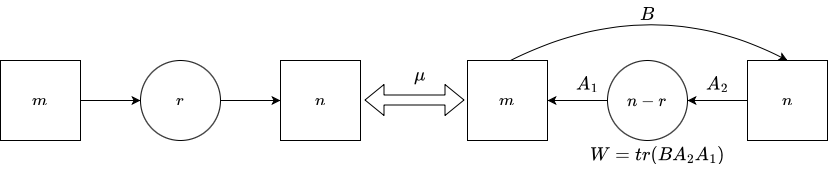
Figure 16: Quivers of fundamental building block related by a mutation at the center node.

The corresponding varieties are total space of $m$-copies of tautological bundles over Grassmannian $S^{\oplus m}\rightarrow Gr(r,n)$ and $m$-copies of dual of the tautological bundles over the dual Grassmannian $(S^{\vee})^{\oplus m}\rightarrow Gr(n-r,n)$.

There is a good torus action $S^{2}=(\mathbb{C}^{*})^{m}\times(\mathbb{C}^{*})^{n}$ on the two varieties. Let $\mathfrak{F}$ be the torus fixed loci of $S^{\oplus m}\rightarrow Gr(r,n)$ and $\mathfrak{F}^{\vee}$ that of $(S^{\vee})^{\oplus m}\rightarrow Gr(n-r,n)$. Adopting the notations and conventions we have used in the above section, one can check that

$$\mathfrak{F}=\{\vec{C}_{[r]}=\{f_{1}<\ldots<f_{r}\}\subset[n]\}\,$$ (5.17)

and

$$\mathfrak{F}^{\vee}=\{\vec{C}_{[n-r]}=\{f_{1}^{\prime}<\ldots<f_{n-r}^{\prime}\}\subset[n]\}\,.$$ (5.18)

The canonical bijective map from $\mathfrak{F}$ to $\mathfrak{F}^{\vee}$ can be defined as

$$\iota^{Gr}:(\vec{C}_{[r]}\subset[n])\rightarrow([n]\backslash\vec{C}_{[r]}\subset[n])\,.$$ (5.19)

Denote the equivariant parameters of $(\mathbb{C}^{*})^{m}$ scaling the fibers of the two varieties by $\eta_{A}$,$A=1,\ldots,m$, and the equivaiant parameters of $(\mathbb{C}^{*})^{n}$ by $\lambda_{F}$, $F=1,\ldots,n$. The equivariant quasimap small ${I}$-function of $S^{\oplus m}\rightarrow Gr(r,n)$, denoted by ${I}^{Gr,S^{2}}(q)$, can be written as follows

$$p^{*}{I}^{Gr,S^{2}}(q)=\sum_{\vec{d}\in\mathbb{Z}^{r}_{\geq 0}}\prod_{I\neq J}^{r}\frac{\prod_{l\leq d_{I}-d_{J}}(x_{I}-x_{J}+l)}{\prod_{l\leq 0}(x_{I}-x_{J}+l)}\prod_{I=1}^{r}\frac{\prod_{A=1}^{m}\prod_{l=0}^{d_{I}-1}(-x_{I}+\eta_{A}-l)}{\prod_{F=1}^{n}\prod_{l=1}^{d_{I}}(x_{I}-\lambda_{F}+l)}q^{\lvert\vec{d}\rvert}\,.$$ (5.20)

The equivariant quasimap small $I$-function of $(S^{\vee})^{\oplus m}\rightarrow Gr(n-r,n)$ denoted by $I^{Gr^{\vee},S^{2}}(q^{\prime})$ is

$$p^{*}{I}^{Gr^{\vee},S^{2}}(q^{\prime})=\sum_{\vec{d}\in\mathbb{Z}^{n-r}_{\leq 0}}\prod_{I\neq J}^{n-r}\frac{\prod_{l\leq d_{I}-d_{J}}(x_{I}-x_{J}+l)}{\prod_{l\leq 0}(x_{I}-x_{J}+l)}\prod_{I=1}^{n-r}\frac{\prod_{A=1}^{m}\prod_{l=1}^{-d_{I}}(-x_{I}+\eta_{A}+l)}{\prod_{F=1}^{n}\prod_{l=1}^{-d_{I}}(-x_{I}+\lambda_{F}+l)}(q^{\prime})^{\lvert\vec{d}\rvert}\,.$$ (5.21)

For an arbitrary $S^{2}$-fixed point $P=(\{f_{1}<\ldots<f_{r}\})\in\mathfrak{F}$, denote the image $\iota^{Gr}(P)$ by $P^{c}=(\{f_{1}^{\prime}<\ldots<f_{n-r}^{\prime}\}=[n]\backslash\vec{C}_{[r]})\in\mathfrak{F}^{\vee}$. The restriction of $I^{Gr,S^{2}}$ to $P$ is

$$p^{*}I^{Gr,S^{2}}(q)\rvert_{P}=\sum_{\vec{d}\in\mathbb{Z}^{r}_{\geq 0}}\prod_{I\neq J}^{r}\frac{\prod_{l\leq d_{I}-d_{J}}(\lambda_{f_{I}}-\lambda_{f_{J}}+l)}{\prod_{l\leq 0}(\lambda_{f_{I}}-\lambda_{f_{J}}+l)}\prod_{I=1}^{r}\frac{\prod_{A=1}^{m}\prod_{l=0}^{d_{I}-1}(-\lambda_{f_{I}}+\eta_{A}-l)}{\prod_{F=1}^{n}\prod_{l=1}^{d_{I}}(\lambda_{f_{I}}-\lambda_{F}+l)}q^{\lvert\vec{d}\rvert}\,.$$ (5.22)

The restriction of $I^{Gr^{\vee},S^{2}}$ to $P^{c}$ is

$$p^{*}I^{Gr^{\vee},S^{2}}(q^{\prime})\rvert_{P^{c}}=\sum_{\vec{d}\in\mathbb{Z}^{n-r}_{\leq 0}}\prod_{I\neq J}^{n-r}\frac{\prod_{l\leq d_{I}-d_{J}}(\lambda_{f_{I}^{\prime}}-\lambda_{f_{J}^{\prime}}+l)}{\prod_{l\leq 0}(\lambda_{f_{I}^{\prime}}-\lambda_{f_{J}^{\prime}}+l)}\prod_{I=1}^{n-r}\frac{\prod_{A=1}^{m}\prod_{l=1}^{-d_{I}}(-\lambda_{f_{I}^{\prime}}+\eta_{A}+l)}{\prod_{F=1}^{n}\prod_{l=1}^{-d_{I}}(-\lambda_{f_{I}^{\prime}}+\lambda_{F}+l)}{q^{\prime}}^{\lvert\vec{d}\rvert}\,.$$ (5.23)

Theorem 5.5 ([Don20, BPZ15]).

1. When $n\geq m+2$, $p^{*}{I}^{Gr,S^{2}}(q)\rvert_{P}=p^{*}{I}^{Gr^{\vee},S^{2}}(q^{-1})\rvert_{P^{c}}$.

2. When $n=m+1$, $p^{*}{I}^{Gr,S^{2}}(q)\rvert_{P}={e}^{(-)^{n-r}q}\,p^{*}{I}^{Gr^{\vee},S^{2}}(q^{-1})\rvert_{P^{c}}$.

3. When $n=m$, $p^{*}{I}^{Gr,S^{2}}(q)\rvert_{P}=(1+(-1)^{n-r}q)^{\sum_{A=1}^{m}\eta_{A}-\sum_{F=1}^{n}\lambda_{F}+n-r}p^{*}{I}^{Gr^{\vee},S^{2}}(q^{-1})\rvert_{P^{c}}$.

5.3 Equivalence of equivariant quasimap small $I$-functions

In this section, we will check the equivalence of quasimap small $I$-functions of a star-shaped quiver and its quiver mutation, and the equivalence of $I$-functions of all mutation-related varieties of $D_{3}$ discussed in Section 2.

5.3.1 Proof for Theorem 1.2: the equivalence between ${I^{\mathcal{X}_{s},S}}$ and ${I^{\tilde{\mathcal{Z}}_{s},S}}$

We firstly utilize the localization theorem to investigate the relation between $I^{\mathcal{X}_{s},S}(\vec{q})\rvert_{P}$ and $I^{\tilde{\mathcal{Z}}_{s},S}(\vec{q}^{\prime})\rvert_{\iota_{s}(P)}$ for each pair of $S$-fixed points $(P,\iota(P))\in\mathfrak{F}_{s}^{b}\times\mathfrak{F}_{s}^{a}$.

Let us first fix a special torus fixed point $P\in\mathfrak{F}_{s}^{b}$ described as follows.

• We first mean to combine the two nodes $6,\,7$. Fix $\vec{C}_{[N_{6}]}=[N_{6}]$ and $\vec{C}_{[N_{7}]}=[N_{7}]$, and then we relabel the integers in the disjoint union $[N_{6}]\sqcup[N_{7}]$ by $1,\ldots,{N_{6}+N_{7}}$. Denote the corresponding equivariant parameters by $\zeta_{I}:=\lambda_{I}$, for $I=1,\ldots,N_{6}$, and $\zeta_{N_{6}+J}:=\lambda_{N_{8}+J}$ for $J=1,\ldots,N_{7}$. Furthermore, the vectors $\vec{n}^{6}$ and $\vec{n}^{7}$ will be together denoted by $\vec{n}\in\mathbb{Z}^{N_{6}+N_{7}}$.

• We choose $\vec{C}_{[N_{5}]}$ to be the first $N_{5}$ integers in $[N_{6}+N_{7}]$ no matter whether $N_{5}\geq N_{6}$ or $N_{5}<N_{6}$, and similarly, we choose $\vec{C}_{[N_{i}]}=[N_{i}]$, for $i=1,\ldots,4$.

Performing a quiver mutation $\mu_{5}$, then we get the image of $P$ under $\iota_{s}$ which can be represented by $(\vec{C}_{[N_{i}]})$ such that

• $\vec{C}_{[N_{6}]}$ and $\vec{C}_{[N_{7}]}$ are the same with those in $P$; we relabel the integers in $[N_{6}],[N_{7}]$ in the same way.

• $\vec{C}_{[N_{5}^{\prime}]}=[N_{6}+N_{7}]\backslash[N_{5}]$, $\vec{C}_{[N_{i}]}=[N_{i}]$, for $i=1,\,2,\,3\,4$.

Proposition 5.6.

For the chosen pair of $S$-fixed points $(P,\iota_{s}(P))\in\mathfrak{F}_{s}^{b}\times\mathfrak{F}_{s}^{a}$, the restricted quasimap small $I$-functions $p^{*}I^{\mathcal{X}_{s},S}\rvert_{P}$ and $p^{*}I^{\widetilde{\mathcal{X}}_{s},S}\rvert_{\iota(P)}$ satisfy the following relation.

1. When $N_{6}+N_{7}\geq N_{3}+N_{4}+2$,

   $$p^{*}I^{\mathcal{X}_{s},S}(\vec{q})\rvert_{P}=p^{*}I^{{\widetilde{\mathcal{Z}}_{s}},S}(\vec{q}^{\prime})\rvert_{\iota_{s}(P)}\,,$$ (5.24)

   and the map between the kähler variables is

   $$q_{5}^{\prime}=q_{5}^{-1},\,q_{6}^{\prime}=q_{6}q_{5},\,q_{7}^{\prime}=q_{7}q_{5},\,q_{i}^{\prime}=q_{i},\text{ for }i\neq 5,6,7\,.$$ (5.25)

2. When $N_{6}+N_{7}=N_{3}+N_{4}+1$,

   $$p^{*}I^{\mathcal{X}_{s},S}(\vec{q})\rvert_{P}=e^{(-1)^{N_{5}^{\prime}}q_{5}}p^{*}I^{{\widetilde{\mathcal{Z}}_{s}},S}(\vec{q}^{\prime})\rvert_{\iota_{s}(P)}\,,$$ (5.26)

   and the map between kähler variables is as (5.25).

3. When $N_{6}+N_{7}=N_{3}+N_{4}$,

   $$p^{*}I^{\mathcal{X}_{s},S}(\vec{q})\rvert_{P}=(1+(-1)^{N_{5}^{\prime}}q_{5})^{\sum_{i=3,4}\sum_{A=1}^{N_{i}}\zeta_{A}-\sum_{F=1}^{N_{6}+N_{7}}\zeta_{F}+N_{5}^{\prime}}p^{*}I^{{\tilde{\mathcal{Z}}_{s}},S}(\vec{q}^{\prime})\rvert_{\iota_{s}(P)}\,,$$ (5.27)

   and the map between kähler variables is

   $$q_{3}^{\prime}=q_{3}(1+(-1)^{N_{5}^{\prime}}q_{5})\,,q_{4}^{\prime}=q_{4}(1+(-1)^{N_{5}^{\prime}}q_{5})\,,q_{5}^{\prime}=q_{5}^{-1}\,,$$

   $$q_{6}^{\prime}=\frac{q_{6}q_{5}}{(1+(-1)^{N_{5}^{\prime}}q_{5})}\,,q_{7}^{\prime}=\frac{q_{7}q_{5}}{(1+(-1)^{N_{5}^{\prime}}q_{5})}\,,q_{i}^{\prime}=q_{i},\text{ for }i=1,2\,.$$ (5.28)

Proof.

By using Lemma 4.4 and isolating the node $5$, which means we fix the integer vectors $\vec{n}^{i}$ for $i\neq 5$ and focus on the terms contributed by the arrows starting from or ending at the node $5$, we transform the $p^{*}I^{\mathcal{X}_{s},S}(\vec{q})\rvert_{P}$ to the following formula

$$p^{*}I^{\mathcal{X}_{s},S}(\vec{q})\rvert_{P}= \sum_{(\vec{n}^{i})\in\operatorname{Eff}_{T}^{s}}(\text{Irrelevant})\mathchoice{\mathbin{\vbox{\hbox{\scalebox{0.5}{$\displaystyle\bullet$}}}}}{\mathbin{\vbox{\hbox{\scalebox{0.5}{$\textstyle\bullet$}}}}}{\mathbin{\vbox{\hbox{\scalebox{0.5}{$\scriptstyle\bullet$}}}}}{\mathbin{\vbox{\hbox{\scalebox{0.5}{$\scriptscriptstyle\bullet$}}}}}\prod_{I=1}^{N_{5}}\left(\prod_{i=3,4}\prod_{A=1}^{N_{i}}\frac{\prod_{l\leq 0}(\zeta_{A}-\zeta_{I}+l)}{\prod_{l\leq n^{i}_{A}-n^{5}_{I}}(\zeta_{A}-\zeta_{I}+l)}\right)$$

$$\prod_{I\neq J}^{N_{5}}\frac{\prod_{l\leq n^{5}_{I}-n^{5}_{J}}(\zeta_{I}-\zeta_{J}+l)}{\prod_{l\leq 0}(\zeta_{I}-\zeta_{J}+l)}\prod_{F=1}^{N_{6}+N_{7}}\prod_{I=1}^{N_{5}}\frac{\prod_{l\leq 0}(\zeta_{I}-\zeta_{F}+l)}{\prod_{l\leq n^{5}_{I}-n_{F}}(\zeta_{I}-\zeta_{F}+l)}\prod_{i\in Q_{0}\backslash Q_{f}}q_{i}^{\lvert\vec{n}^{i}\rvert}\,,$$ (5.29)

where the irrelevant part represents the remaining factors away from the center node. Notice that $m_{I}:=n^{5}_{I}-n_{I}\geq 0$. Replace $n_{I}^{5}=m_{I}+n_{I}$, and we can transform $p^{*}I^{\mathcal{X}_{s},S}(\vec{q})$ to the following formula,

$$p^{*}I^{\mathcal{X}_{s},S}(\vec{q})\rvert_{P}= \sum_{\vec{m}\in\mathbb{Z}^{N_{5}}_{\geq 0}}(\text{Irrelevant})\mathchoice{\mathbin{\vbox{\hbox{\scalebox{0.5}{$\displaystyle\bullet$}}}}}{\mathbin{\vbox{\hbox{\scalebox{0.5}{$\textstyle\bullet$}}}}}{\mathbin{\vbox{\hbox{\scalebox{0.5}{$\scriptstyle\bullet$}}}}}{\mathbin{\vbox{\hbox{\scalebox{0.5}{$\scriptscriptstyle\bullet$}}}}}\prod_{I=1}^{N_{5}}\left(\prod_{i=3,4}\prod_{A=1}^{N_{i}}\frac{\prod_{l\leq 0}(\zeta_{A}-\zeta_{I}+l)}{\prod_{l\leq n^{i}_{A}-n_{I}-m_{I}}(\zeta_{A}-\zeta_{I}+l)}\right)\prod_{i\in Q_{0}\backslash Q_{f},i\neq 5}q_{i}^{\lvert\vec{n}^{i}\rvert}$$

$$\prod_{I\neq J}^{N_{5}}\frac{\prod_{l\leq n_{I}-n_{J}+m_{I}-m_{J}}(\zeta_{I}-\zeta_{J}+l)}{\prod_{l\leq 0}(\zeta_{I}-\zeta_{J}+l)}\prod_{F=1}^{N_{6}+N_{7}}\prod_{I=1}^{N_{5}}\frac{\prod_{l\leq 0}(\zeta_{I}-\zeta_{F}+l)}{\prod_{l\leq m_{I}+n_{I}-n_{F}}(\zeta_{I}-\zeta_{F}+l)}q_{5}^{\lvert\vec{m}\rvert+\sum_{I=1}^{N_{5}}n_{I}}\,.$$ (5.30)

Do more combinatorics, and we can transform the above $I$-function to

$$p^{*}I^{\mathcal{X}_{s},S}(\vec{q})\rvert_{P}= \sum_{\vec{m}\in\mathbb{Z}^{N_{5}}_{\geq 0}}(\text{Irrelevant})\mathchoice{\mathbin{\vbox{\hbox{\scalebox{0.5}{$\displaystyle\bullet$}}}}}{\mathbin{\vbox{\hbox{\scalebox{0.5}{$\textstyle\bullet$}}}}}{\mathbin{\vbox{\hbox{\scalebox{0.5}{$\scriptstyle\bullet$}}}}}{\mathbin{\vbox{\hbox{\scalebox{0.5}{$\scriptscriptstyle\bullet$}}}}}\prod_{i=3,4}\prod_{A=1}^{N_{i}}\prod_{I=1}^{N_{5}}\frac{\prod_{l\leq n^{i}_{A}-n_{I}}(\zeta_{A}-\zeta_{I}+l)}{\prod_{l\leq n^{i}_{A}-n_{I}-m_{I}}(\zeta_{A}-\zeta_{I}+l)}q_{5}^{\lvert\vec{m}\rvert+\sum_{I=1}^{N_{5}}n_{I}}$$ (5.31a)

$$\prod_{I\neq J}^{N_{5}}\frac{\prod_{l\leq n_{I}-n_{J}+m_{I}-m_{J}}(\zeta_{I}-\zeta_{J}+l)}{\prod_{l\leq n_{I}-n_{J}}(\zeta_{I}-\zeta_{J}+l)}\prod_{F=1}^{N_{6}+N_{7}}\prod_{I=1}^{N_{5}}\frac{\prod_{l\leq n_{I}-n_{F}}(\zeta_{I}-\zeta_{F}+l)}{\prod_{l\leq m_{I}+n_{I}-n_{F}}(\zeta_{I}-\zeta_{F}+l)}$$ (5.31b)

$$\prod_{i=3,4}\prod_{A=1}^{N_{i}}\prod_{I=1}^{N_{5}}\frac{\prod_{l\leq 0}(\zeta_{A}-\zeta_{I}+l)}{\prod_{l\leq n^{i}_{A}-n_{I}}(\zeta_{A}-\zeta_{I}+l)}\prod_{I=1}^{N_{5}}\prod_{F=N_{5}+1}^{N_{6}+N_{7}}\frac{\prod_{l\leq 0}(\zeta_{I}-\zeta_{F}+l)}{\prod_{l\leq n_{I}-n_{F}}(\zeta_{I}-\zeta_{F}+l)}$$ (5.31c)

Notice that for fixed $\vec{n}^{i}$, $i\neq 5$, the subequation (5.31c) is fixed, and subequations (5.31a) and (5.31b) can be viewed as degree $\vec{m}$-term of the equavariant quasimap small $I$-function of $S^{N_{3}+N_{4}}\rightarrow Gr(N_{5},N_{6}+N_{7})$, if we pretend that the equivariant parameters of $(\mathbb{C}^{*})^{N_{3}+N_{4}}$ are $\zeta_{A}+n^{i}_{A}$, $i=3,4,A=1,\ldots,N_{i}$, and equivariant parameters of $(\mathbb{C}^{*})^{N_{6}+N_{7}}$ are $\zeta_{F}+n_{F}$, $F=1,\ldots,N_{6}+N_{7}$.

Being restricted to $\iota_{s}(P)$, the ingredients are $x^{i}_{I}\rvert_{\iota_{s}(P)}=\zeta_{I}$, for $i=1,2,3,4$, $x^{5}_{I}\rvert_{\iota_{s}(P)}=\zeta_{N_{5}+I}$, $x^{6}_{I}\rvert_{\iota_{s}(P)}=\zeta_{I}$, $x^{7}_{I}\rvert_{\iota_{s}(P)}=\zeta_{N_{6}+I}$. The restriction of quasimap-small $I$-function $p^{*}I^{\widetilde{\mathcal{Z}}_{s},S^{1}}(\vec{q}^{\prime})$ to $\iota_{s}(P)$ is

$$p^{*}I^{\widetilde{\mathcal{Z}}_{s},S}(\vec{q}^{\prime})\rvert_{\iota_{s}(P)} =\sum_{(\vec{n}^{i})\in\operatorname{Eff}_{T}^{ms}}(\text{Irrelevant})\mathchoice{\mathbin{\vbox{\hbox{\scalebox{0.5}{$\displaystyle\bullet$}}}}}{\mathbin{\vbox{\hbox{\scalebox{0.5}{$\textstyle\bullet$}}}}}{\mathbin{\vbox{\hbox{\scalebox{0.5}{$\scriptstyle\bullet$}}}}}{\mathbin{\vbox{\hbox{\scalebox{0.5}{$\scriptscriptstyle\bullet$}}}}}\prod_{i=3,4}\prod_{A=1}^{N_{i}}\prod_{I=1}^{N_{5}^{\prime}}\frac{\prod_{l\leq n^{i}_{A}-n^{5}_{I}}(\zeta_{A}-\zeta_{N_{5}+I}+l)}{\prod_{l\leq 0}(\zeta_{A}-\zeta_{N_{5}+I}+l)}$$

$$\prod_{I\neq J}^{N_{5}^{\prime}}\frac{\prod_{l\leq n^{5}_{I}-n^{5}_{J}}(\zeta_{N_{5}+I}-\zeta_{N_{5}+J}+l)}{\prod_{l\leq 0}(\zeta_{N_{5}+I}-\zeta_{N_{5}+J}+l)}\prod_{F=1}^{N_{6}+N_{7}}\prod_{I=1}^{N_{5}^{\prime}}\frac{\prod_{l\leq 0}(-\zeta_{N_{5}+I}+\zeta_{F}+l)}{\prod_{l\leq-n^{5}_{I}+n_{F}}(-\zeta_{N_{5}+I}+\zeta_{F}+l)}$$

$$\prod_{i=3,4}\prod_{A=1}^{N_{i}}\prod_{F=1}^{N_{6}+N_{7}}\frac{\prod_{l\leq 0}(\zeta_{A}-\zeta_{F}+l)}{\prod_{l\leq n^{i}_{A}-n_{F}}(\zeta_{A}-\zeta_{F}+l)}\prod_{i\in Q_{0}\backslash Q_{f}}(q_{i}^{\prime})^{\lvert\vec{n}^{i}\rvert}\,.$$ (5.32)

Like the above strategy, we must have $m_{I}=-n^{5}_{I}+n_{N_{5}+I}\geq 0$. Otherwise, the corresponding term would vanish. Replace $n_{I}^{5}=n_{N_{5}+I}-m_{I}$, and we transform the above $I$-function to

$$p^{*}I^{\tilde{\mathcal{Z}}_{s},S}(\vec{q}^{\prime})\rvert_{\iota_{s}(P)}=\sum_{\vec{m}^{i}\in\mathbb{Z}^{N_{5}^{\prime}}_{\geq 0}}(\text{Irrelevant})\mathchoice{\mathbin{\vbox{\hbox{\scalebox{0.5}{$\displaystyle\bullet$}}}}}{\mathbin{\vbox{\hbox{\scalebox{0.5}{$\textstyle\bullet$}}}}}{\mathbin{\vbox{\hbox{\scalebox{0.5}{$\scriptstyle\bullet$}}}}}{\mathbin{\vbox{\hbox{\scalebox{0.5}{$\scriptscriptstyle\bullet$}}}}}\prod_{I\neq J}^{N_{5}^{\prime}}\frac{\prod_{l\leq n_{N_{5}+I}-n_{N_{5}+J}-m_{I}+m_{J}}(\zeta_{N_{5}+I}-\zeta_{N_{5}+J}+l)}{\prod_{l\leq n_{N_{5}+I}-n_{N_{5}+J}}(\zeta_{N_{5}+I}-\zeta_{N_{5}+J}+l)}$$ (5.33a)

$$\prod_{i=3,4}\prod_{A=1}^{N_{i}}\prod_{I=1}^{N_{5}^{\prime}}\frac{\prod_{l\leq n^{i}_{A}-n_{N_{5}+I}+m_{I}}(\zeta_{A}-\zeta_{N_{5}+I}+l)}{\prod_{l\leq n^{i}_{A}-n_{N_{5}+I}}(\zeta_{A}-\zeta_{N_{5}+I}+l)}\prod_{F=1}^{N_{6}+N_{7}}\prod_{I=1}^{N_{5}^{\prime}}\frac{\prod_{l\leq-n_{N_{5}+I}+n_{F}}(-\zeta_{N_{5}+I}+\zeta_{F}+l)}{\prod_{l\leq-n_{N_{5}+I}+n_{F}+m_{I}}(-\zeta_{N_{5}+I}+\zeta_{F}+l)}$$ (5.33b)

$$\prod_{i=3,4}\prod_{A=1}^{N_{i}}\prod_{I=1}^{N_{5}}\frac{\prod_{l\leq 0}(\zeta_{A}-\zeta_{I}+l)}{\prod_{l\leq n^{i}_{A}-n_{I}}(\zeta_{A}-\zeta_{I}+l)}\prod_{I=1}^{N_{5}}\prod_{F=N_{5}+1}^{N_{6}+N_{7}}\frac{\prod_{l\leq 0}(\zeta_{I}-\zeta_{F}+l)}{\prod_{l\leq n_{I}-n_{F}}(\zeta_{I}-\zeta_{F}+l)}(q_{5}^{\prime})^{-\lvert\vec{m}\rvert+\sum_{I=1}^{N_{5}^{\prime}}n_{N_{5}+I}}.$$ (5.33c)

We find that for fixed $\vec{n}^{i},i\neq 5$, subequation (5.33c) is fixed, and subequations (5.33a) and (5.33b) can be viewed as degree $\vec{m}$ term of equivariant quasimap small $I$-function of $(S^{\vee})^{N_{3}+N_{4}}\rightarrow Gr(N_{5}^{\prime},N_{6}+N_{7})$, if we pretend that $n^{i}_{A}+\zeta_{A}$, $i=3,4,\,A=1,\ldots,N_{i}$ are equivariant parameters of $(\mathbb{C}^{*})^{N_{3}+N_{4}}$ action on their fiber and $n_{F}+\zeta_{F}$ are equivariant parameters of $(\mathbb{C}^{*})^{N_{6}+N_{7}}$ action on $Gr(N_{5}^{\prime},N_{6}+N_{7})$.

The irrelevant parts of $p^{*}I^{\mathcal{X}_{s},S}\rvert_{P}$ and $p^{*}I^{\tilde{\mathcal{Z}}_{s},S}\rvert_{\iota_{s}(P)}$ are equal, and subequations (5.31c) and (5.33c) are equal for fixed $\vec{n}^{i},\,i\neq 5$. Subequations (5.31a) (5.31b) and subequations (5.33a) (5.33b) are related by the fundamental building block Theorem 5.5. Hence, we have proved the proposition. ∎

Notice that the above proposition can be extended to any pair of $S$-fixed points $(P,\iota_{s}(P))\in\mathfrak{F}_{s}^{b}\times\mathfrak{F}_{s}^{a}$. Therefore, we have proved the Theorem 1.2 for the general star-shaped quiver by localization.

Corollary 1.4 is a natural result of the Theorem 1.2.

5.3.2 Proof for Theorem 1.5

Let us first clarify what we need to do to prove the Theorem 1.5.

• The relation of $I$-functions $I^{\mathcal{X}_{0},S^{1}}$ and $I^{\mathcal{Z}_{1},S^{1}}$ has been done in Corollary 1.4.

• The relations among $I^{\mathcal{X}_{4},S^{1}}\leftrightarrow I^{\mathcal{X}_{5},S^{1}}\leftrightarrow I^{\mathcal{X}_{6},S^{1}}$ and the relations among $I^{\mathcal{X}_{7},S^{1}}\leftrightarrow I^{\mathcal{X}_{8},S^{1}}\leftrightarrow I^{\mathcal{X}_{9},S^{1}}$ are the same type, performing quiver mutations at the nodes 1 or 2 with the remaining nodes unchanged. We may view those locally as a mutation to an $A$-type quiver, which was discussed in our previous work [Zha21].

• The equivalence between $I^{\mathcal{X}_{6},S^{1}}\leftrightarrow I^{\mathcal{X}_{7},S^{1}}$ is natural since we know that $\mathcal{X}_{6}$ and $\mathcal{X}_{7}$ are isomorphic. However, we need to change the signs of chern roots $x^{i}_{I}$ to identify the two $I$-functions.

• The equivalence between $I^{\mathcal{X}_{9},S^{1}}\leftrightarrow I^{\mathcal{X}_{0},S^{1}}$ can be derived from the fact that the two quiver varieties are equal by exchanging nodes $1$ and $2$.

• The proofs for the equivalence between $I^{\mathcal{Z}_{3},S^{1}}\leftrightarrow I^{\mathcal{X}_{4},S^{1}}$ and that between $I^{\mathcal{X}_{0},S^{1}}\leftrightarrow I^{\mathcal{Z}_{1},S^{1}}$ are the same, since $\mathcal{X}_{0}$ is isomorphic to $\mathcal{X}_{4}$ and $\mathcal{Z}_{1}$ is isomorphic to $\mathcal{Z}_{3}$.

• The equivalence between $I^{\mathcal{Z}_{2},S^{1}}\leftrightarrow I^{\mathcal{Z}_{3},S^{1}}$ can be derived from that between $I^{\mathcal{Z}_{1},S^{1}}\leftrightarrow I^{\mathcal{Z}_{2},S^{1}}$, since $\mathcal{Z}_{3}$ is isomorphic to $\mathcal{Z}_{1}$.

We will only need to prove the equivalence $I^{\mathcal{Z}_{1},S^{1}}\leftrightarrow I^{\mathcal{Z}_{2},S^{1}}$ in detail, but we will make the change of variables clear when needed for other easy cases.

Proof for the equivalence between $\mathbf{I^{\mathcal{Z}_{1},S^{1}}}$ and $\mathbf{I^{\mathcal{Z}_{2},S^{1}}}.$ By the same strategy as the previous subsection, we are led to investigate the relation of the restriction of the two $I$-functions to any pair of $S^{1}$-fixed points in $\mathfrak{F}_{1}\times\mathfrak{F}_{2}$.

Consider a special torus fixed point $P_{1}$,

$$P_{1}=([N_{1}],{[N_{2}]},\vec{C}_{[N_{3}^{\prime}]}),\,\,\vec{C}_{[N_{3}^{\prime}]}=[N_{4}]\backslash[N_{3}]\,.$$ (5.34)

Its image $\iota_{1}(P_{1})\in\mathfrak{F}_{2}$ can be represented by

$$P_{2}:=\iota_{1}(P_{1})=([N_{4}]\backslash[N_{1}],[N_{2}],[N_{4}]\backslash[N_{3}])\,.$$ (5.35)

Lemma 5.7.

The restrictions of $I^{\mathcal{Z}_{1},S^{1}}$ and $I^{\mathcal{Z}_{2},S^{1}}$ to the pair of $S^{1}$-fixed points $(P_{1},P_{2})$ satisfy the following relation,

$$p^{*}I^{\mathcal{Z}_{1},S^{1}}(\vec{q})\rvert_{P_{1}}=p^{*}I^{\mathcal{Z}_{2},S^{1}}(\vec{q}^{\prime})\rvert_{P_{2}}\,$$ (5.36)

via the variable change

$$q_{1}^{\prime}=q_{1}^{-1},\,q_{2}^{\prime}=q_{2},\,q_{3}^{\prime}=q_{3}.$$ (5.37)

Proof.

The restrictions of ingredients of $\mathcal{Z}_{1}$ to $P_{1}$ are $x_{I}^{i}\rvert_{P_{1}}=\lambda_{I}$ for $i=1,2$, and $x^{3}_{I}\rvert_{P_{1}}=\lambda_{N_{3}+I}$. The restriction of $I^{\mathcal{Z}_{1},S^{1}}$ to $P_{1}$ is

$$p^{*}I^{\mathcal{Z}_{1},S^{1}]}(\vec{q})\rvert_{P_{1}} =\sum_{(\vec{n}^{i})\in\operatorname{Eff}_{T}^{1}}\prod_{i=1,2}\prod_{I\neq J}^{N_{i}}\frac{\prod_{l\leq n^{i}_{I}-n^{i}_{J}}(\lambda_{I}-\lambda_{J}+l)}{\prod_{l\leq 0}(\lambda_{I}-\lambda_{J}+l)}\prod_{\begin{subarray}{c}I,J=1\\ I\neq J\end{subarray}}^{N_{3}^{\prime}}\frac{\prod_{l\leq n^{3}_{I}-n^{3}_{J}}(\lambda_{N_{3}+I}-\lambda_{N_{3}+J}+l)}{\prod_{l\leq 0}(\lambda_{N_{3}+I}-\lambda_{N_{3}+J}+l)}$$

$$\prod_{F=1}^{N_{4}}\prod_{i=1}^{2}\prod_{I=1}^{N_{i}}\frac{\prod_{l\leq 0}(\lambda_{I}-\lambda_{F}+l)}{\prod_{l\leq n^{i}_{I}}(\lambda_{I}-\lambda_{F}+l)}\prod_{I=1}^{N_{3}^{\prime}}\frac{\prod_{l\leq 0}(-\lambda_{N_{3}^{\prime}+I}+\lambda_{F}+l)}{\prod_{l\leq-n^{3}_{I}}(-\lambda_{N_{3}^{\prime}+I}+\lambda_{F}+l)}$$

$$\prod_{I=1}^{N_{3}^{\prime}}\prod_{i=1}^{2}\prod_{J=1}^{N_{i}}\frac{\prod_{l\leq n^{i}_{J}-n^{3}_{I}}(\lambda_{J}-\lambda_{N_{3}+I}+l)}{\prod_{l\leq 0}(\lambda_{J}-\lambda_{N_{3}+I}+l)}\prod_{i=1}^{3}q_{i}^{\lvert\vec{n}^{i}\rvert}\,.$$ (5.38)

We do some combinatorics to the $I^{\mathcal{Z}_{1},S^{1}}(\vec{q})\rvert_{P_{1}}$ by freezing the nodes $3$ and $4$. Then we can transform $I^{\mathcal{Z}_{1},S^{1}}(\vec{q})\rvert_{P_{1}}$ to the following formula.

$$p^{*}I^{\mathcal{Z}_{1},S^{1}}(\vec{q})\rvert_{P_{1}} =\sum_{(\vec{n}^{i})\in\operatorname{Eff}_{T}^{1}}\prod_{\begin{subarray}{c}I,J=1\\ I\neq J\end{subarray}}^{N_{2}}\frac{\prod_{l\leq n^{2}_{I}-n^{2}_{J}}(\lambda_{I}-\lambda_{J}+l)}{\prod_{l\leq 0}(\lambda_{I}-\lambda_{J}+l)}\prod_{\begin{subarray}{c}I,J=1\\ I\neq J\end{subarray}}^{N_{3}^{\prime}}\frac{\prod_{l\leq n^{3}_{I}-n^{3}_{J}}(\lambda_{N_{3}+I}-\lambda_{N_{3}+J}+l)}{\prod_{l\leq 0}(\lambda_{N_{3}+I}-\lambda_{N_{3}+J}+l)}$$ (5.39a)

$$\prod_{F=1}^{N_{4}}\prod_{I=1}^{N_{2}}\frac{\prod_{l\leq 0}(\lambda_{I}-\lambda_{F}+l)}{\prod_{l\leq n^{2}_{I}}(\lambda_{I}-\lambda_{F}+l)}\prod_{J=1}^{N_{3}^{\prime}}\prod_{I=1}^{N_{1}}\frac{\prod_{l\leq 0}(-\lambda_{N_{3}+J}+\lambda_{N_{1}+I}+l)}{\prod_{l\leq-n^{3}_{J}}(-\lambda_{N_{3}+J}+\lambda_{N_{1}+I}+l)}$$ (5.39b)

$$\prod_{J=1}^{N_{3}^{\prime}}\prod_{I=1}^{N_{2}}\frac{\prod_{l\leq n^{2}_{I}-n^{3}_{J}}(\lambda_{I}-\lambda_{N_{3}+J}+l)}{\prod_{l\leq 0}(\lambda_{I}-\lambda_{N_{3}+J}+l)}$$ (5.39c)

$$\prod_{\begin{subarray}{c}I,J=1\\ I\neq J\end{subarray}}^{N_{1}}\frac{\prod_{l\leq n^{1}_{I}-n^{1}_{J}}(\lambda_{I}-\lambda_{J}+l)}{\prod_{l\leq 0}(\lambda_{I}-\lambda_{J}+l)}\prod_{I=1}^{N_{1}}\frac{\prod_{J=1}^{N_{3}^{\prime}}\prod_{l=1}^{n^{1}_{I}}(\lambda_{I}-\lambda_{N_{3}+J}-n^{3}_{J}+l)}{\prod_{F=1}^{N_{4}}\prod_{l=1}^{n^{1}_{I}}(\lambda_{I}-\lambda_{F}+l)}\prod_{i=1}^{3}q_{i}^{\lvert\vec{n}^{i}\rvert}.$$ (5.39d)

In the above formula, for fixed $\vec{n}^{2},\,\vec{n}^{3}$, sub-equations (5.39a) (5.39b) and (5.39c) are fixed, and sub-equation (5.39d) is the restriction of quasimap small $I$-function of $(S^{\vee})^{\oplus N_{3}^{\prime}}\rightarrow Gr(N_{1},N_{4})$ to the torus fixed point $([N_{1}]\subset[N_{4}])$ if we pretend that $\lambda_{N_{3}+J}+p_{J}$, $J=1,\ldots,N_{3}^{\prime}$ and $\lambda_{F}$, $F=1,\ldots,N_{4}$ are equivariant parameters of $(\mathbb{C}^{*})^{N_{3}^{\prime}}\times(\mathbb{C}^{*})^{N_{4}}$ action.

Consider the restriction of $I^{\mathcal{Z}_{2},S^{1}}(\vec{q})$ to $P_{2}$, $x_{I}^{1}\rvert_{P_{2}}=\lambda_{N_{1}+I}$, $x^{2}_{I}\rvert_{P_{2}}=\lambda_{I}$, $x^{3}_{I}\rvert_{P_{2}}=\lambda_{N_{3}+I}$. Then

$$p^{*}I^{\mathcal{Z}_{2},S^{1}}(\vec{q}^{\prime})\rvert_{P_{2}} =\sum_{(\vec{n}^{i})\in\operatorname{Eff}_{T}^{2}}\prod_{\begin{subarray}{c}I,J=1\\ I\neq J\end{subarray}}^{N_{2}}\frac{\prod_{l\leq n^{1}_{I}-n^{1}_{J}}(\lambda_{I}-\lambda_{J}+l)}{\prod_{l\leq 0}(\lambda_{I}-\lambda_{J}+l)}\prod_{\begin{subarray}{c}I,J=1\\ I\neq J\end{subarray}}^{N_{3}^{\prime}}\frac{\prod_{l\leq n^{3}_{I}-n^{3}_{J}}(\lambda_{N_{3}+I}-\lambda_{N_{3}+J}+l)}{\prod_{l\leq 0}(\lambda_{N_{3}+I}-\lambda_{N_{3}+J}+l)}$$

$$\prod_{\begin{subarray}{c}I,J=1\\ I\neq J\end{subarray}}^{N_{2}}\frac{\prod_{l\leq n^{1}_{I}-n^{1}_{J}}(\lambda_{N_{1}+I}-\lambda_{N_{1}+J}+l)}{\prod_{l\leq 0}(\lambda_{N_{1}+I}-\lambda_{N_{1}+J}+l)}\prod_{I=1}^{N_{2}}\prod_{J=1}^{N_{3}^{\prime}}\frac{\prod_{l\leq 0}(\lambda_{N_{1}+I}-\lambda_{N_{3}+J}+l)}{\prod_{l\leq n^{1}_{I}-n^{3}_{J}}(\lambda_{N_{1}+I}-\lambda_{N_{3}+J}+l)}$$

$$\prod_{F=1}^{N_{4}}\left(\prod_{I=1}^{N_{2}}\frac{\prod_{l\leq 0}(-\lambda_{N_{1}+I}+\lambda_{F}+l)}{\prod_{l\leq-n^{1}_{I}}(-\lambda_{N_{1}+I}+\lambda_{F}+l)}\prod_{I=1}^{N_{2}}\frac{\prod_{l\leq 0}(\lambda_{I}-\lambda_{F}+l)}{\prod_{l\leq n^{2}_{I}}(\lambda_{J}-\lambda_{F}+l)}\right)$$

$$\prod_{I=1}^{N_{2}}\prod_{J=1}^{N_{3}^{\prime}}\frac{\prod_{l\leq n^{2}_{I}-n^{3}_{J}}(\lambda_{I}-\lambda_{N_{3}+J}+l)}{\prod_{l\leq 0}(\lambda_{I}-\lambda_{N_{3}+J}+l)}\prod_{i=1}^{3}(q_{i}^{\prime})^{\lvert\vec{n}^{i}\rvert}.$$ (5.40)

Freezing the nodes $3$ and $4$, we can transform $p^{*}I^{\mathcal{Z}_{2},S^{1}}(\vec{q}^{\prime})\rvert_{P_{2}}$ to the following formula.

$$p^{*}I^{\mathcal{Z}_{2},S^{1}}(\vec{q}^{\prime})\rvert_{P_{2}} =\sum_{(\vec{n}^{i})\in\operatorname{Eff}_{T}^{2}}\prod_{\begin{subarray}{c}I,J=1\\ I\neq J\end{subarray}}^{N_{2}}\frac{\prod_{l\leq n^{2}_{I}-n^{2}_{J}}(\lambda_{I}-\lambda_{J}+l)}{\prod_{l\leq 0}(\lambda_{I}-\lambda_{J}+l)}\prod_{\begin{subarray}{c}I,J=1\\ I\neq J\end{subarray}}^{N_{3}^{\prime}}\frac{\prod_{l\leq n^{3}_{I}-n^{3}_{J}}(\lambda_{N_{3}+I}-\lambda_{N_{3}+J}+l)}{\prod_{l\leq 0}(\lambda_{N_{3}+I}-\lambda_{N_{3}+J}+l)}$$ (5.41a)

$$\prod_{F=1}^{N_{4}}\prod_{I=1}^{N_{2}}\frac{\prod_{l\leq 0}(\lambda_{I}-\lambda_{F}+l)}{\prod_{l\leq n^{2}_{I}}(\lambda_{J}-\lambda_{F}+l)}\prod_{I=1}^{N_{2}}\prod_{J=1}^{N_{3}^{\prime}}\frac{\prod_{l\leq n^{2}_{I}-n^{3}_{J}}(\lambda_{I}-\lambda_{N_{3}+J}+l)}{\prod_{l\leq 0}(\lambda_{I}-\lambda_{N_{3}+J}+l)}$$ (5.41b)

$$\prod_{I=1}^{N_{2}}\prod_{J=1}^{N_{3}^{\prime}}\frac{\prod_{l\leq 0}(\lambda_{N_{1}+I}-\lambda_{N_{3}+J}+l)}{\prod_{l\leq-n^{3}_{J}}(\lambda_{N_{1}+I}-\lambda_{N_{3}+J}+l)}\prod_{i=1}^{3}(q_{i}^{\prime})^{\lvert\vec{n}^{i}\rvert}$$ (5.41c)

$$\prod_{\begin{subarray}{c}I,J=1\\ I\neq J\end{subarray}}^{N_{2}}\frac{\prod_{l\leq n^{1}_{I}-n^{1}_{J}}(\lambda_{N_{1}+I}-\lambda_{N_{1}+J}+l)}{\prod_{l\leq 0}(\lambda_{N_{1}+I}-\lambda_{N_{1}+J}+l)}\prod_{I=1}^{N_{2}}\frac{\prod_{J=1}^{N_{3}^{\prime}}\prod_{l=0}^{-n^{1}_{I}-1}(\lambda_{N_{1}+I}-\lambda_{N_{3}+J}-n^{3}_{J}-l)}{\prod_{F=1}^{N_{4}}\prod_{l=1}^{-n^{1}_{I}}(-\lambda_{N_{1}+I}+\lambda_{F}+l)}\,.$$ (5.41d)

Again for fixed $\vec{n}^{2},\vec{n}^{3}$, the sub-equations (5.41a)(5.41b)(5.41c) are fixed. The sub-equation (5.41a) is the degree $\vec{n}^{1}$ term of the equivariant quasimap small $I$-function of $S^{\oplus(N_{3}^{\prime})}\rightarrow Gr(N_{2},N_{4})$ being restricted to the $(\mathbb{C}^{*})^{N_{3}^{\prime}}\times(\mathbb{C}^{*})^{N_{4}}$-fixed point $([N_{4}]\backslash[N_{1}]\subseteq[N_{4}])$, if we pretend that $\lambda_{N_{1}+J}+p_{J}$ $J=1,\ldots,N_{3}^{\prime}$ and $\lambda_{F}$ $F=1,\ldots,N_{4}$ are equivariant parameters for $(\mathbb{C}^{*})^{N_{3}^{\prime}}\times(\mathbb{C}^{*})^{N_{4}}$-action.

One may find that the sub-equations (5.39d) and (5.41d) are different from the $I$-functions of the two varieties in the fundamental building block and their equivariant parameters differ by a sign $\pm$. The reason is that we are using different quiver diagrams and hence different GIT quotients to represent $S^{N_{3}^{\prime}}\rightarrow Gr(N_{1},N_{4})$ and $(S^{\vee})^{N_{3}^{\prime}}\rightarrow Gr(N_{2},N_{4})$. Explicitly, the quiver diagrams here are as Figure 17; they are different in orientation from the diagrams in Figure 16 but define the same quiver varieties.

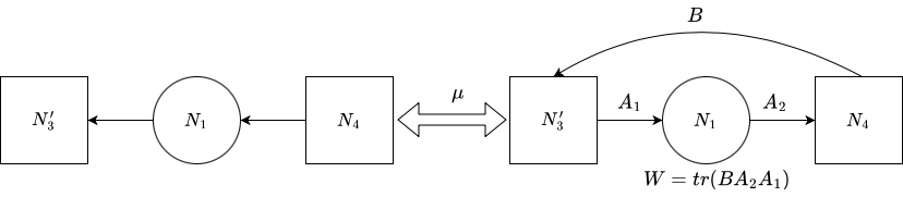
Figure 17: Another quiver diagram for fundamental building block.

Compare $p^{*}I^{\mathcal{Z}_{1},S^{1}}(\vec{q})\rvert_{P_{1}}$ with $p^{*}I^{\mathcal{Z}_{2},S^{1}}(\vec{q}^{\prime})\rvert_{P_{2}}$, and we find that for fixed $\vec{n}^{2},\vec{n}^{3}$, sub-equations (5.41a)(5.41b)(5.41c) are exactly equal to sub-equations (5.39a)(5.39b)(5.39c). Sub-equations (5.39d) is equal to (5.41d) for a degree $\lvert\vec{n}^{1}\rvert$ by Theorem 5.5 item 1. Hence, we have proved the Lemma. ∎

By extending the above procedure to any pair of torus fixed points in $\mathfrak{F}_{1}\times\mathfrak{F}_{2}$, we can conclude the quiver mutation $\mu_{1}$ preserves the equivariant quasimap small $I$-functions for $\mathcal{Z}_{1}$ and $\mathcal{Z}_{2}$:

$$p^{*}I^{\mathcal{Z}_{1},S^{1}}(q_{1},q_{2},q_{3})=p^{*}I^{\mathcal{Z}_{2},S^{1}}(q_{1}^{-1},q_{2},q_{3})\,.$$ (5.42)

Combining the first map of kähler variables in (1.8), we can prove that the kähler variables of $\mathcal{X}_{0}$ are mapped to

$$((1+(-1)^{N_{3}^{\prime}}q_{3})q_{1})^{-1},\,(1+(-1)^{N_{3}^{\prime}}q_{3})q_{2},\,q_{3}^{-1}\,,$$ (5.43)

via the cluster transformation $\mu_{1}\mu_{3}$.

The equivalence between $\mathbf{I^{\mathcal{Z}_{2},S^{1}}(q_{1},q_{2},q_{3})}$ and $\mathbf{I^{\mathcal{Z}_{3},S^{1}}(q_{1},q_{2},q_{3})}$. In our examples, the variety $\mathcal{Z}_{1}$ is isomorphic to $\mathcal{Z}_{3}$ and their $I$-functions are related by the following relations,

$$I^{\mathcal{Z}_{3},S^{1}}(q_{1},q_{2},q_{3})=I^{\mathcal{Z}_{1},S^{1}}(q_{2}^{-1},q_{1}^{-1},q_{3}^{-1})\,,$$ (5.44)

via the change of chern roots and equivariant parameters

$$x^{1}_{I}\rightarrow-x^{2}_{I},\text{ for }I=1,\ldots,N_{2}\,,$$

$$x^{2}_{J}\rightarrow-x^{1}_{J},\text{ for }J=1,\ldots,N_{1}\,,$$

$$x^{3}_{I}\rightarrow-x^{3}_{I},\text{ for }I=1,\ldots,N_{3}^{\prime},\,$$

$$\lambda_{F}\rightarrow-\lambda_{F},\text{ for }F=1,\ldots,{N_{4}}\,.$$ (5.45)

Hence, we can derive the relation between $I^{\mathcal{Z}_{2},S^{1}}$ and $I^{\mathcal{Z}_{3},S^{1}}$,

$$I^{\mathcal{Z}_{3},S^{1}}(q_{2}^{-1},q_{1},q_{3}^{-1})=I^{\mathcal{Z}_{2},S^{1}}(q_{1},q_{2},q_{3})\,,$$ (5.46)

via change of chern roots and parameters in Equation (5.3.2).

Equivalence between $\mathbf{{I^{\mathcal{Z}_{3},S^{1}}(q_{1},q_{2},q_{3})}}$ and $\mathbf{{I^{\mathcal{X}_{4},S^{1}}(q_{1},q_{2},q_{3})}}$. Since $\mathcal{Z}_{3}$ is isomorphic to $\mathcal{Z}_{1}$ and $\mathcal{X}_{4}$ is isomorphic to $\mathcal{X}_{0}$, the relation between $\mathcal{Z}_{3}$ and $\mathcal{X}_{4}$ can be derived directly from Corollary 1.4.

$$p^{*}I^{\mathcal{Z}_{3},S^{1}}(q_{1},q_{2},q_{3})=(1+(-1)^{N_{3}^{\prime}}q_{3})^{\sum_{I=1}^{N_{2}}x^{1}_{I}+\sum_{I=1}^{N_{1}}x^{2}_{I}-\sum_{F=1}^{N_{4}}\lambda_{F}-N_{4}+N_{3}}I^{\mathcal{X}_{4},S^{1}}(q_{1}^{\prime},q_{2}^{\prime},q_{3}^{\prime})\,,$$ (5.47)

with variable change

$$q_{1}^{\prime}=(1+(-1)^{N_{3}^{\prime}}q_{3})q_{1},\,q_{2}^{\prime}=(1+(-1)^{N_{3}^{\prime}}q_{3})q_{2},\,q_{3}^{\prime}=q_{3}^{-1}\,.$$ (5.48)

Remark 5.8.

Notice that the transformation of the kähler variables (5.46) does not match that of the Seiberg Duality Conjecture 1.1, which is unexpected. The reason is that in Figure 15 (a), the phase has to be chosen as $\sigma_{3}<0$, otherwise $V_{4}^{ss}\neq V^{s}_{4}$. Performing the quiver mutation $\mu_{3}$ to Figure 15 (a), we return to Figure 14. The correct phase for the resulting GIT must be as (2.27) where $\sigma_{3}>0$ so that the varieties $\mathcal{X}_{4}$ and $\mathcal{Z}_{3}$ satisfy the Seiberg Duality Conjecture perfectly. Such choice for phase $\sigma_{3}>0$ to construct $\mathcal{Z}_{3}$ makes the relation between $\mathcal{Z}_{2}$ and $\mathcal{Z}_{3}$ beyond the expectation of the Seiberg Duality Conjecture. Fortunately, we can still make their equivariant quasimap small $I$-functions equal thanks to their geometric relation: $\mathcal{Z}_{3}$ is isomorphic to $\mathcal{Z}_{1}$.

If we choose $\sigma_{3}<0$ in (2.27), we can still construct an algebraic variety $\tilde{\mathcal{Z}}_{3}$ in the following way. Choose another character $\tilde{\theta}_{3}$ of $G_{3}$ as

$$\tilde{\sigma}_{1}<0,\tilde{\sigma}_{2}<0,\tilde{\sigma}_{3}<0,$$ (5.49)

and we have

$$Z(dW_{3})^{ss}_{\tilde{\theta}}=\{A_{3}=0,\begin{bmatrix}B_{1}&B_{2}\end{bmatrix}\begin{bmatrix}A_{1}\\ A_{2}\end{bmatrix}=0,\,\rvert\,\,B_{1},B_{2},\begin{bmatrix}A_{1}\\ A_{2}\end{bmatrix}\text{non-degenerate}\}\,.$$ (5.50)

Denote its GIT quotient by $\tilde{\mathcal{Z}_{3}}:=Z(dW_{3})\sslash_{\tilde{\theta}_{3}}G_{3}$. Consider another quiver diagram

Denote its input data by $(U_{3},G_{3},\tilde{\theta}_{3})$, and then

$$U^{ss}_{3\,\,\tilde{\theta}_{3}}(G_{3})=\{B_{1},B_{2},\begin{bmatrix}A_{1}\\ A_{2}\end{bmatrix}\text{non-degenerate}\}\,.$$ (5.51)

$\tilde{\mathcal{Z}}_{3}$ is a subvariety in $U_{3}\sslash_{\tilde{\theta}_{3}}G_{3}$. The two varieties $\tilde{\mathcal{Z}}_{3}$ and $\mathcal{Z}_{3}$ are birational by choosing different phases of an algebraic group $G_{3}$, and we expect that their qusimap small $I$-functions are equal up to analytic continuation, as discussed in the very beginning of the introduction.

The following equivalences between $I$-functions are easy, and readers can derive the following relations by the above strategy. We will list them without further computation and pay more attention to the change of kähler variables.

The equivalence among $\mathbf{I^{\mathcal{X}_{4},S^{1}}(q_{1},q_{2},q_{3})}$, $\mathbf{{I^{\mathcal{X}_{5},S^{1}}(q_{1},q_{2},q_{3})}}$, and $\mathbf{{I^{\mathcal{X}_{6},S^{1}}(q_{1},q_{2},q_{3})}}$. The only node connected to the gauge node $1$ is node $3$. Isolating the two nodes $1$ and $3$, the quiver mutation is reduced to the relation between $Gr(N_{2},N_{3})$ and $Gr(N_{3}-N_{2},N_{3})$. One can use the combinatorics we used for the $A_{n}$ case to prove the following result.

$$I^{\mathcal{X}_{4},S^{1}}(q_{1},q_{2},q_{3})=I^{\mathcal{X}_{5},S^{1}}(q_{1}^{-1},q_{2},q_{3}q_{1})\,.$$ (5.52)

The relation between ${I^{\mathcal{X}_{5},S^{1}}(q_{1},q_{2},q_{3})}$ and ${I^{\mathcal{X}_{6},S^{1}}(q_{1},q_{2},q_{3})}$ can be reduced to the relation of $I$-functions between $Gr(N_{1},N_{3})$ and $Gr(N_{3}-N_{1},N_{3})$. Hence, we have

$$I^{\mathcal{X}_{6},S^{1}}(q_{1},q_{2},q_{3})=I^{\mathcal{X}_{5},S^{1}}(q_{1},q_{2}^{-1},q_{3}q_{2})\,.$$ (5.53)

The equivalence between $\mathbf{I^{\mathcal{X}_{6},S^{1}}(q_{1},q_{2},q_{3})}$ and $\mathbf{I^{\mathcal{X}_{7},S^{1}}(q_{1},q_{2},q_{3})}.$ The quiver mutation at node $3$ makes $\mathcal{X}_{6}$ isomorphic to $\mathcal{X}_{7}$, and their equivariant quasimap small $I$-functions can be identified directly via change of chern roots and equivariant parameters.

$$I^{\mathcal{X}_{6},S^{1}}(q_{1},q_{2},q_{3})=I^{\mathcal{X}_{7},S^{1}}(q_{1}^{-1},q_{2}^{-1},q_{3}^{-1})$$ (5.54)

via a change of chern roots and equivariant parameters

$$x^{i}_{I}\rightarrow=-x^{i}_{I},\,i=1,\,2,\,3,\,\lambda_{F}\rightarrow-\lambda_{F},\,F=1,\ldots,N_{4}.$$ (5.55)

The equivalence among $\mathbf{I^{\mathcal{X}_{7},S^{1}}(q_{1},q_{2},q_{3})}$, $\mathbf{{I^{\mathcal{X}_{8},S^{1}}(q_{1},q_{2},q_{3})}}$, and $\mathbf{{I^{\mathcal{X}_{9},S^{1}}(q_{1},q_{2},q_{3})}}$. The relation between $I^{\mathcal{X}_{8},S^{1}}$ and $I^{\mathcal{X}_{7},S^{1}}$ is precisely the same as that between $I^{\mathcal{X}_{5},S^{1}}$ and $I^{\mathcal{X}_{6},S^{1}}$,

$$I^{\mathcal{X}_{8},S^{1}}(q_{1},q_{2},q_{3})=I^{\mathcal{X}_{7},S^{1}}(q_{1}^{-1},q_{2},q_{3}q_{1})\,.$$ (5.56)

The relation between $I^{\mathcal{X}_{8},S^{1}}$ and $I^{\mathcal{X}_{9},S^{1}}$ is precisely the same as that between $I^{\mathcal{X}_{5},S^{1}}$ and $I^{\mathcal{X}_{4},S^{1}}$,

$$I^{\mathcal{X}_{9},S^{1}}(q_{1},q_{2},q_{3})=I^{\mathcal{X}_{8},S^{1}}(q_{1},q_{2}^{-1},q_{3}q_{2})\,.$$ (5.57)

By exchanging nodes $1$ and $2$, which is equivalent to exchanging variables $q_{1}$ and $q_{2}$, and transforming chern roots:

$$x^{1}_{I}\rightarrow x^{2}_{I},I=1,\ldots N_{2},\,\,x^{2}_{J}\rightarrow x^{1}_{J},J=1,\ldots N_{1}\,.$$ (5.58)

we recover $I^{\mathcal{X}_{0},S^{1}}$,

$$I^{\mathcal{X}_{9},S^{1}}(q_{2},q_{1},q_{3})=I^{\mathcal{X}_{0},S^{1}}(q_{1},q_{2},q_{3})\,.$$ (5.59)

Until now, we have proved the Theorem 1.5.

References

- [AB84] M.F. Atiyah and R. Bott, The moment map and equivariant cohomology, Topology 23 (1984), no. 1, 1–28.
- [Beh97] K. Behrend, Gromov-Witten invariants in algebraic geometry, Invent. Math. 127 (1997), no. 3, 601–617. MR 1431140
- [BF97] K. Behrend and B. Fantechi, The intrinsic normal cone, Invent. Math. 128 (1997), no. 1, 45–88. MR 1437495
- [BFZ05] Arkady Berenstein, Sergey Fomin, and Andrei Zelevinsky, Cluster algebras iii: Upper bounds and double bruhat cells, Duke Mathematical Journal 126 (2005), no. 1, 1–52.
- [BG09] Jim Bryan and Tom Graber, The crepant resolution conjecture, Algebraic geometry—Seattle 2005. Part 1, Proc. Sympos. Pure Math., vol. 80, Amer. Math. Soc., Providence, RI, 2009, pp. 23–42. MR 2483931
- [BPZ15] Francesco Benini, Daniel S Park, and Peng Zhao, Cluster algebras from dualities of 2d quiver gauge theories, Communications in Mathematical Physics 340 (2015), no. 1, 47–104.
- [CCFK15] Daewoong Cheong, Ionuţ Ciocan-Fontanine, and Bumsig Kim, Orbifold quasimap theory, Math. Ann. 363 (2015), no. 3-4, 777–816. MR 3412343
- [CFFG+18] Ionut Ciocan-Fontanine, David Favero, Jérémy Guéré, Bumsig Kim, and Mark Shoemaker, Fundamental factorization of a glsm, part i: Construction, arXiv preprint arXiv:1802.05247 (2018).
- [CFK14] Ionuţ Ciocan-Fontanine and Bumsig Kim, Wall-crossing in genus zero quasimap theory and mirror maps, Algebr. Geom. 1 (2014), no. 4, 400–448. MR 3272909
- [CFK16] , Big -functions, Development of moduli theory—Kyoto 2013, Adv. Stud. Pure Math., vol. 69, Math. Soc. Japan, [Tokyo], 2016, pp. 323–347. MR 3586512
- [CFKM14] Ionuţ Ciocan-Fontanine, Bumsig Kim, and Davesh Maulik, Stable quasimaps to GIT quotients, J. Geom. Phys. 75 (2014), 17–47. MR 3126932
- [CIJ18] Tom Coates, Hiroshi Iritani, and Yunfeng Jiang, The crepant transformation conjecture for toric complete intersections, Adv. Math. 329 (2018), 1002–1087. MR 3783433
- [CIR14] Alessandro Chiodo, Hiroshi Iritani, and Yongbin Ruan, Landau-Ginzburg/Calabi-Yau correspondence, global mirror symmetry and Orlov equivalence, Publ. Math. Inst. Hautes Études Sci. 119 (2014), 127–216. MR 3210178
- [CK99] David A. Cox and Sheldon Katz, Mirror symmetry and algebraic geometry, Mathematical Surveys and Monographs, vol. 68, American Mathematical Society, Providence, RI, 1999. MR 1677117
- [CR10] Alessandro Chiodo and Yongbin Ruan, Landau-Ginzburg/Calabi-Yau correspondence for quintic three-folds via symplectic transformations, Invent. Math. 182 (2010), no. 1, 117–165. MR 2672282
- [Don20] Hai Dong, I-funciton in Grassmannian Duality, Ph.D Thesis of Peking university (2020).
- [DWZ08] Harm Derksen, Jerzy Weyman, and Andrei Zelevinsky, Quivers with potentials and their representations. I. Mutations, Selecta Math. (N.S.) 14 (2008), no. 1, 59–119. MR 2480710
- [DWZ10] , Quivers with potentials and their representations II: applications to cluster algebras, J. Amer. Math. Soc. 23 (2010), no. 3, 749–790. MR 2629987
- [ESm89] Geir Ellingsrud and Stein Arild Strø mme, On the Chow ring of a geometric quotient, Ann. of Math. (2) 130 (1989), no. 1, 159–187. MR 1005610
- [EW12] Gonzalez Eduardo and Chris T. Woodward, A wall-crossing formula for gromov-witten invariants under variation of git quotient, arXiv preprint arXiv:1208.1727 (2012).
- [FJR18] Huijun Fan, Tyler J. Jarvis, and Yongbin Ruan, A mathematical theory of the gauged linear sigma model, Geom. Topol. 22 (2018), no. 1, 235–303. MR 3720344
- [FK20] David Favero and Bumsig Kim, Fundamental factorization of a glsm, part i: Construction, arXiv preprint arXiv:2006.12182 (2020).
- [FZ02] Sergey Fomin and Andrei Zelevinsky, Cluster algebras. I. Foundations, J. Amer. Math. Soc. 15 (2002), no. 2, 497–529. MR 1887642
- [FZ03] , Cluster algebras. II. Finite type classification, Invent. Math. 154 (2003), no. 1, 63–121. MR 2004457
- [FZ07] , Cluster algebras. IV. Coefficients, Compos. Math. 143 (2007), no. 1, 112–164. MR 2295199
- [GLF16] Jaume Gomis and Bruno Le Floch, M2-brane surface operators and gauge theory dualities in toda, Journal of High Energy Physics 2016 (2016), no. 4, 1–111.
- [GP99] T. Graber and R. Pandharipande, Localization of virtual classes, Invent. Math. 135 (1999), no. 2, 487–518. MR 1666787
- [Hor13] Kentaro Hori, Duality in two-dimensional (2, 2) supersymmetric non-abelian gauge theories, Journal of High Energy Physics 2013 (2013), no. 10, 1–76.
- [HT07] Kentaro Hori and David Tong, Aspects of non-abelian gauge dynamics in two-dimensional theories, Journal of High Energy Physics 2007 (2007), no. 05, 079.
- [IMRS21] Hiroshi Iritani, Todor Milanov, Yongbin Ruan, and Yefeng Shen, Gromov-Witten theory of quotients of Fermat Calabi-Yau varieties, Mem. Amer. Math. Soc. 269 (2021), no. 1310, v+92. MR 4223045
- [Kir05] Frances Kirwan, Refinements of the Morse stratification of the normsquare of the moment map, The breadth of symplectic and Poisson geometry, Progr. Math., vol. 232, Birkhäuser Boston, Boston, MA, 2005, pp. 327–362. MR 2103011
- [Kir16] Alexander Kirillov, Jr., Quiver representations and quiver varieties, Graduate Studies in Mathematics, vol. 174, American Mathematical Society, Providence, RI, 2016. MR 3526103
- [KL18] Young-Hoon Kiem and Jun Li, Quantum singularity theory via cosection localization, arXiv preprint arXiv:1806.00116 (2018).
- [LLW10] Yuan-Pin Lee, Hui-Wen Lin, and Chin-Lung Wang, Flops, motives, and invariance of quantum rings, Ann. of Math. (2) 172 (2010), no. 1, 243–290. MR 2680420
- [LR01] An-Min Li and Yongbin Ruan, Symplectic surgery and Gromov-Witten invariants of Calabi-Yau 3-folds, Invent. Math. 145 (2001), no. 1, 151–218. MR 1839289
- [LT98] Jun Li and Gang Tian, Virtual moduli cycles and Gromov-Witten invariants of algebraic varieties, J. Amer. Math. Soc. 11 (1998), no. 1, 119–174. MR 1467172
- [Mar00] Shaun Martin, Symplectic quotients by a nonabelian group and by its maximal torus, arXiv preprint math/0001002 (2000).
- [Rua06] Yongbin Ruan, The cohomology ring of crepant resolutions of orbifolds, Gromov-Witten theory of spin curves and orbifolds, Contemp. Math., vol. 403, Amer. Math. Soc., Providence, RI, 2006, pp. 117–126. MR 2234886
- [Rua17] , Nonabelian gauged linear sigma model, Chin. Ann. Math. Ser. B 38 (2017), no. 4, 963–984. MR 3673177
- [Web18] Rachel Webb, The Abelian-Nonabelian Correspondence for I-functions, arXiv preprint arXiv:1804.07786 (2018).
- [Web21] , Abelianization and Quantum Lefschetz for Orbifold Quasimap I-functions, arXiv preprint arXiv:2109.12223 (2021).
- [Wit97] Edward Witten, Phases of theories in two dimensions, Mirror symmetry, II, AMS/IP Stud. Adv. Math., vol. 1, Amer. Math. Soc., Providence, RI, 1997, pp. 143–211. MR 1416338
- [Zha21] Yingchun Zhang, Gromov-witten theory of type quiver varieties and seiberg duality, arXiv preprint arXiv:2112.11812 (2021).