Enhancing Exploration in Latent Space Bayesian Optimization

Abstract

Latent Space Bayesian Optimization (LSBO) combines generative models, typically Variational Autoencoders (VAE), with Bayesian Optimization (BO) to generate de novo objects of interest. However, LSBO faces challenges due to the mismatch between the objectives of BO and VAE, resulting in poor extrapolation capabilities. In this paper, we propose novel contributions to enhance LSBO efficiency and overcome this challenge. We first introduce the concept of latent consistency/inconsistency as a crucial problem in LSBO, arising from the BO-VAE mismatch. To address this, we propose the Latent Consistent Aware-Acquisition Function (LCA-AF) that leverages consistent regions in LSBO. Additionally, we present LCA-VAE, a novel VAE method that generates a latent space with increased consistent points, improving BO’s extrapolation capabilities. Combining LCA-VAE and LCA-AF, we develop LCA-LSBO. Experimental evaluations validate the improved performance of LCA-LSBO in image generation and de-novo chemical design tasks, showcasing its enhanced extrapolation capabilities in LSBO. Our approach achieves high sample-efficiency and effective exploration, emphasizing the significance of addressing latent consistency and leveraging LCA-VAE in LSBO.

1 Introduction

Bayesian Optimization (BO) is a machine learning technique for optimizing expensive-to-evaluate black-box (BB) functions. A key property of BO is to consider the exploration-exploitation trade-off, i.e., finding a trade-off between exploring new regions of the search space and exploiting the knowledge gained from previous evaluations. BO is effective when the search space is represented in a low-dimensional vector space. However, applying BO to high-dimensional data or structural data such as chemical compounds is challenging. To overcome this challenge, a method called Latent Space Bayesian Optimization (LSBO) has been proposed [1], in which the LS of the high-dimensional/structure data is identified by using generative models such as Variational Autoencoder (VAE) and BO is performed in the LS. Figure 1 illustrates LSBO.

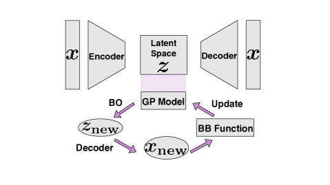
Figure 1: The illustration of LSBO process, where $\bm{x}$ and $\bm{z}$ indicate input and latent variables, respectively (see §2 for notations). The aim of LSBO is to find the latent variable that maximizes the BB function when it is decoded by the encoder by using a surrogate model, such as Gaussian Process (GP), fitted in the LS of the trained VAE. In LSBO, the following process is repeated: i) a new latent variable $\bm{z}_{\rm new}$ is selected by acquisition function (AF), ii) $\bm{z}_{\rm new}$ is decoded to $\bm{x}_{\rm new}$, iii) the BB function is evaluated at $\bm{x}_{\rm new}$, and iv) the surrogate model in the LS is updated by incorporating $\bm{z}_{\rm new}$ and its BB function value. More details are provided in §2.2.

Unfortunately, a simple combination of VAE and BO usually does not yield satisfactory results. This can be attributed to the mismatch between the objectives of VAE and LSBO. The main objective of VAE is to generate instances that closely resemble the training instances by sampling from the dense region in the LS. On the other hand, LSBO is primarily focused on generating de-novo instances that are typically dissimilar to the training instances and are sampled from sparse regions in the LS especially in its exploration phase. Therefore, to enable LSBO to effectively perform exploration and exploitation, it is indispensable to identify a LS that can resolve this mismatch.

In this study, we examine two critical issues in LSBO that stem from the mismatch. The first issue is what we refer to as latent consistency/inconsistency. Consider a situation where a single point in the LS is first decoded and then it is again encoded into the LS. In this situation, we refer to a point in the LS as latent consistent when the point obtained by passing through the decoder and encoder of the VAE is located in the same point, whereas we refer to a point as latent inconsistent when the two points are located differently. Figure 2 illustrates the notions of latent consistency/inconsistency.

In LSBO, since a BB function evaluation is performed after decoding the evaluation point in the LS, if the evaluation point is latent inconsistent, the obtained BB function value will no longer match that of the actual evaluation point. To address the issue of latent inconsistency, we propose a new type of acquisition functions (AFs) for LSBO called latent consistent-aware AF (LCA-AF). The LCA-AF enables us to focus on searching only for latent consistent points in the LS in LSBO, thereby avoiding the aforementioned latent inconsistency issue.

The second issue is the narrow latent consistent regions in the LS, which hinders the exploration of a wide search space in LSBO. When conducting exploration in LSBO, it involves exploring regions where training instances do not exist, namely, the low-density regions in the LS. However, these low-density regions often exhibit latent inconsistency, making it difficult to perform sufficient exploration. Figure 3(B) indicates the density of latent consistent points in a LS obtained by a standard VAE trained with the standard normal distribution as its prior.

We propose a new VAE method in order to address the issue of limited latent consistent regions. We refer to this method as the latent consistent-aware VAE (LCA-VAE). The fundamental idea of LCA-VAE is to train a VAE such that the regions to be explored in the LS have latent consistency. By using LCA-VAE, it becomes possible to expand the latent consistent region in the LS, enabling LSBO to conduct exploration over a wider range. Figure 3(D) indicates the density of latent consistent points in a LS obtained by the proposed LCA-VAE, indicating that the latent consistency is widened compared with Fig. 3(B).

The key contributions of our paper are as follows:

1. We introduce the concept of latent consistency/inconsistency as an important problem in existing LSBO. To address the problem, we propose a new AF for LSBO, called LCA-AF, which enables exploration in the latent consistent region.

2. We introduce LCA-VAE, a novel VAE method that can generate a LS which contains larger number of latent consistency points, thereby improving BO’s exploration capabilities.

3. We combine LCA-VAE and LCA-AF to develop a new LSBO method, which we call, Latent Consistency Aware-LSBO (LCA-LSBO). Through image generation and de-novo chemical design experiments, we validate the improved performance of LCA-LSBO, demonstrating its enhanced LSBO capabilities.

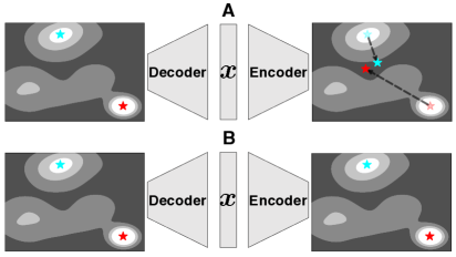
Figure 2: The plots represent 2-dimensional LS. The brighter regions in each figure denotes promising regions with higher BB function values from which we want to sample new instances in LSBO. In A, after latent variables are sampled from the promising regions, by decoding then and encoding them back, they traverse the LS as in the black dotted-lines, demonstrating that they are latent inconsistent. On the other hand, in B, when new latent variables are sampled from promising regions, they came back to the same locations in the LS after decoding and encoding, indicating their latent consistency.

1.1 Related Works

The VAE [2] is one of the most popular generative models with many applications such as image generation [3], anomaly detection [4], and denoising [5]. The BO has also been intensively studied as a BB function optimization method, particularly for problems where the evaluation cost of BB functions is high [6]. The LSBO was first introduced for de novo molecular design in [1]. Then, the LSBO was applied to various problems such as neural architecture search [7], image generation [8], material discovery [9], and protein design [10].

Many studies have been conducted to improve the LSBO method. First, in the seminal work in [1], the authors first proposed a method that simply combines the standard VAE and the standard BO, which we refer to as the vanilla VAE. Additionally, they proposed an approach to make the LS more suitable for label prediction by performing label (e.g., chemical property) prediction on the LS during VAE training, which we refer to as the predictor VAE. As an other approach to incorporate label information into LSBO, Richards and Groener [11] suggested to use conditional $\beta$-VAE. To improve the validity of instances generated by LSBO, Griffiths and Hernández-Lobato [12] proposed a specific method in the context of molecular design problems. Siivola et al. [13] conducted a study to evaluate how factors such as the dimension of the LS and the choice of acquisition function affect the performances of LSBO.

The above methods are still sub-optimal because the new information obtained through BO iteration(s) is not incorporated into the VAE. Tripp et al. [14] proposed a weighted retraining approach where the VAE is retrained by an updated training set after BO iteration(s), where the weights of the instances in the updated training set are set to be proportional to their label information. Taking different direction, [15] tackles the problem of high-dimensional search space of LSBO problems and propose a local optimization based LSBO approach. Furthermore, Grosnit et al. [16] introduced a metric learning approach while retraining the VAE. Berthelot et al. [8] proposed invariant data augmentations to improve the quality of the LS and make it more amenable to BO.

Finally, let us mention several existing studies that have been discussed in different contexts than the LSBO but are relevant to our proposed LCA-LSBO method. The similar notion of latent consistency has been discussed for enhancing the disentanglement of the LS for image generation task [17]. In the context of BO, several methods have been developed to handle high-dimensional or strctured data. In particular, an approach called manifold GP can be interpreted as a method for conducting BO in a LS [18]. As we describe later, we retrain the VAE by incorporating artificially generated latent variables, which allows us to adapt the LS for the LSBO task. This approach can also be regarded as a variant of adaptive data augmentation (see, e.g., [19]).

2 Preliminaries and Problem Definition

Here, we present preliminary information and problem definition.

2.1 VAEs

A VAE consists of an encoder network $f_{\phi}^{\rm enc}:{\mathcal{X}}\to{\mathcal{Z}}$ and a decoder network $f_{\theta}^{\rm dec}:{\mathcal{Z}}\to{\mathcal{X}}$ where ${\mathcal{X}}$ is the domain of input variables $\bm{x}$ and ${\mathcal{Z}}$ is the domain of latent variables $\bm{z}$, where $\phi$ and $\theta$ are the parameters of the encoder and the decoder, respectively. In VAEs, input variables $\bm{x}$ and latent variables $\bm{z}$ are considered as random variables. Let $p_{\theta}(\bm{x})$ and $p_{\theta}(\bm{z})$ be the probability functions of $\bm{x}$ and $\bm{z}$, respectively, where $\theta$ is the set of parameters for characterizing the probabilities. The encoder network $f_{\phi}^{\rm enc}$ is formulated as a conditional probability $q_{\phi}(\bm{z}\mid\bm{x})$, which is considered as an approximation of $p_{\theta}(\bm{z}\mid\bm{x})$, whereas the decoder network $f_{\theta}^{\rm dec}$ is formulated as a conditional probability $p_{\theta}(\bm{x}\mid\bm{z})$.

A VAE is trained by maximizing

$$J_{\rm VAE}(\phi,\theta)=\mathbb{E}_{\bm{z}\sim q_{\phi}(\bm{z}\mid\bm{x})}\log p_{\theta}(\bm{x}\mid\bm{z})-\beta D_{\rm KL}\left(q_{\phi}(\bm{z}\mid\bm{x})\|p_{\theta}(\bm{z})\right),$$ (1)

where $\mathbb{E}_{\bm{z}\sim q_{\phi}(\bm{z}\mid\bm{x})}$ is an expectation operator for random variables $\bm{z}$ that follows the conditional distribution $q_{\phi}(\bm{z}\mid\bm{x})$, $D_{\rm KL}(\cdot\|\cdot)$ is Kullback Leibler (KL) divergence between two distributions, and $\beta>0$ is a hyperparameter to trade-off the balance between the two terms. In (1), the prior distribution of the latent variables $p_{\theta}(\bm{z})$ is usually set as a multivariate normal distribution ${\mathcal{N}}(\bm{0},I)$. When $\beta=1$, the objective function is reduced to that of the standard VAEs and it can be interpreted as a lower bound of the log likelihood of the input distribution $p_{\theta}(\bm{x})$. On the other hand, VAEs with $\beta\neq 1$ is called $\beta$-VAE [20].

The conditional probability $q_{\phi}(\bm{z}\mid\bm{x})$ in the encoder network is formulated as follows. Given an input variable $\bm{x}$, the latent variable $\bm{z}$ is encoded as $\bm{z}=\bm{\mu}_{\phi}(\bm{x})+\sigma_{\phi}(\bm{x})\bm{\varepsilon},~{}\bm{\varepsilon}\sim{\mathcal{N}}(\bm{0},I),$ where $\bm{\mu}_{\phi}:{\mathcal{X}}\to{\mathcal{Z}}$ and $\sigma_{\phi}:{\mathcal{X}}\to\mathbb{R}^{+}$ represent the mean and the standard deviation of the latent variable corresponding to $\bm{x}$, respectively, and they are implemented together in the encoder network $f_{\phi}^{\rm enc}$ with the trainable parameters $\phi$, whereas $\bm{\varepsilon}$ is a random variable sampled from ${\mathcal{N}}(\bm{0},I)$. Given a latent variable $\bm{z}$, using the conditional probability $p_{\theta}(\bm{x}\mid\bm{z})$ in the decoder network $f_{\theta}^{\rm dec}$, an input variable $\hat{\bm{x}}$ is generated as $\hat{\bm{x}}\sim p_{\theta}(\bm{x}\mid\bm{z}).$

2.2 LSBO

In LSBO, we start with a large number of unlabeled instances $\{\bm{x}_{i}\}_{i\in[{\mathcal{U}}]}$ and a small number of labeled instances $\{(\bm{x}_{i},y_{i})\}_{i\in[{\mathcal{L}}]}$, where $\bm{x}_{i}\in{\mathcal{X}}$ is an input object such as chemical compound and $y_{i}\in{\mathcal{Y}}\subseteq\mathbb{R}$ is the label of the input object $\bm{x}_{i}$ such as drug-likeness of the chemical compound $\bm{x}_{i}$. Here, the sets of indices of the unlabeled and labeled instances are denoted as ${\mathcal{U}}$ and ${\mathcal{L}}$, respectively, and ${\mathcal{Y}}\subseteq\mathbb{R}$ indicates the space of the label which is assumed to be scalar in this study.

A BO is used for a BB function optimization problem when an evaluation of the BB function is expensive (in terms of time, money, etc.). Let us denote the BB function as $f^{\rm BB}:{\mathcal{X}}\to{\mathcal{Y}}$. The goal of a BO is to find $\bm{x}\in{\mathcal{X}}$ that maximizes the BB function with as small number of BB function evaluations as possible. The basic idea of BOs is to use a surrogate model for the BB function, and it is common to employ a GP model as the surrogate model. If a good surrogate GP model on the input object space ${\mathcal{X}}$ can be constructed using the labeled instances $\{(\bm{x}_{i},y_{i})\}_{i\in{\mathcal{L}}}$, the predictive distribution of the label can be obtained for each input object with unknown labels. Using the predictive distributions, one or more candidates of input objects whose labels are predicted to be greater than the current maximum value $\max_{i\in{\mathcal{L}}}y_{i}$ can be selected. After evaluating the BB function for the candidate input objects, the labeled set ${\mathcal{L}}$ and the GP surrogate model are updated. This process is repeated until we obtain the maximum value or use out the available resource budget.

Unfortunately, it is often difficult to develop a good GP surrogate model on the input object space ${\mathcal{X}}$ when $\bm{x}$ is a high-dimensional complex object such as chemical compound. The basic idea of LSBO is to first train a VAE using unlabeled set ${\mathcal{U}}$, and then fit a GP surrogate model on the LS ${\mathcal{Z}}$ in the trained VAE. Fitting a GP model on the LS ${\mathcal{Z}}$ can be easier than fitting it on the input object space ${\mathcal{X}}$ because the former is lower-dimensional vector space. Let us denote a GP model in the LS by $f^{\rm GP}:{\mathcal{Z}}\to{\mathcal{Y}}$ which is fitted by using $\{(f_{\phi}^{\rm enc}(\bm{x}_{i}),y_{i})\}_{i\in{\mathcal{L}}}$. At each iteration of LSBO, by applying the AF to the predictive distributions obtained by the GP surrogate model on the LS, the latent variable that maximizes the AF, i.e., $\bm{{z}}_{i^{\prime}}=\mathop{\rm argmax}_{\bm{z}\in{\mathcal{Z}}}f^{\rm AF}(\bm{z})$ can be obtained. Using the decoder, an input object $\bm{x}_{i^{\prime}}=f_{\theta}^{\rm dec}(\bm{{z}}_{i^{\prime}})$ is obtained as the target of the next BB function evaluation. The labeled set is then updated as ${\mathcal{L}}\leftarrow{\mathcal{L}}\cup\{i^{\prime}\}$ and the GP model is also updated accordingly. Here, an optional but useful step is to retrain the VAE model by using the updated dataset ${\mathcal{L}}\cup{\mathcal{U}}$ in order to incorporate the new information to the model[14, 16]. As in the standard BO, this process is repeated until we obtain the maximum value or use out the available resource budget. For example, in a chemical compound design problem, the LSBO is used to find a chemical compound with desired property.

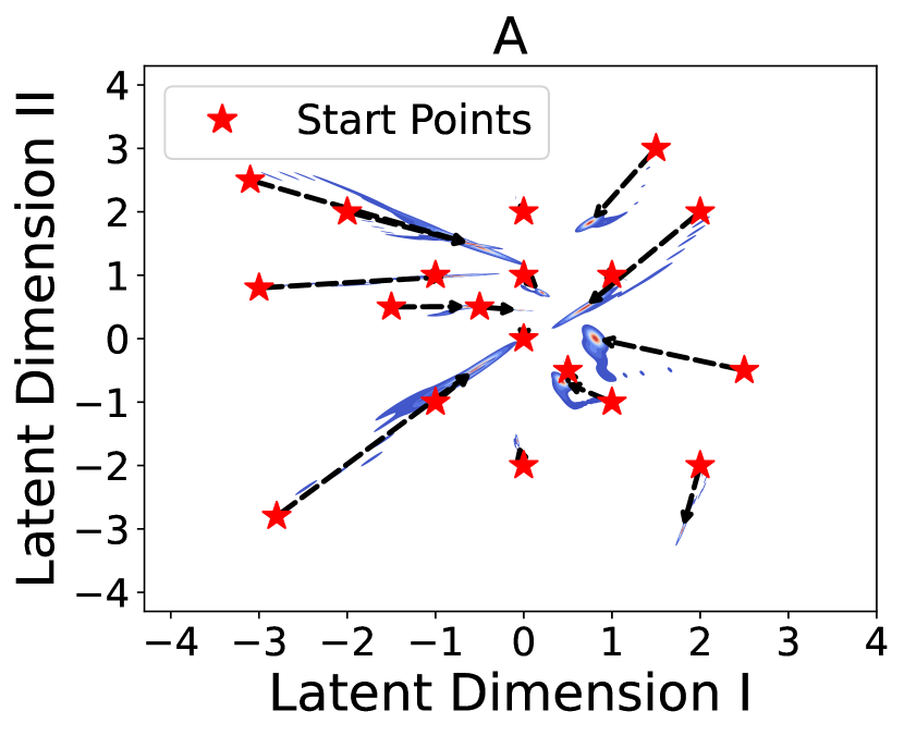
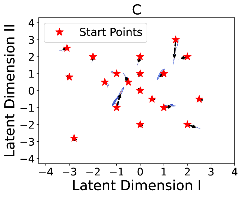
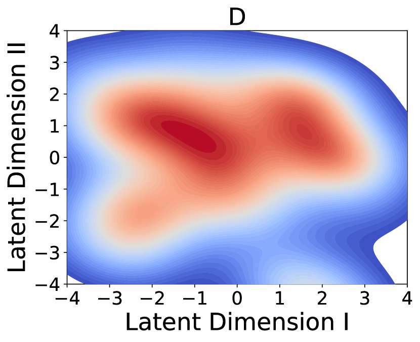
Figure 3: Latent consistent points in 2-dimensional LS of VAE trained on MNIST dataset [21]. A and B show the LS of the standard VAE while C and D show the LS of proposed LCA-VAE. Black dotted arrows in A and C indicate how the latent variables traverse in the LS when we repeat encoding and decoding many times. In A, many latent variables traverse extensively, whereas in C, it can be observed that most latent variables remain in almost the same position. LSBO behaves as intended only in latent consistent regions. Therefore, when the latent consistent regions are narrow as in B, the exploration capability of LSBO is limited. On the other hand, in D, the proposed LCA-VAE has expanded the latent consistent regions, enabling more extensive exploration.

Algorithm 1 Succesive cycles of $\bm{z}$

1:VAE encoder $f^{\text{enc}}_{\phi}$, VAE decoder $f^{\text{dec}}_{\theta}$, the number of cycles $M$, latent variable $\bm{z}$

2:Initialize an empty set $\bm{Z}$

3:for $j=1$ to $M$ do

4:     ${\bm{z}}^{j}\leftarrow f^{\text{enc}}_{\phi}(f^{\text{dec}}_{\theta}(\bm{z}))$

5:     Add ${\bm{z}}^{j}$ to $\bm{Z}$

6:     $\bm{z}\leftarrow{\bm{z}}^{j}$

7:end for

8:return $\bm{Z}$

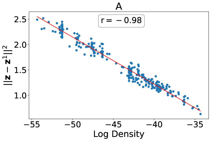
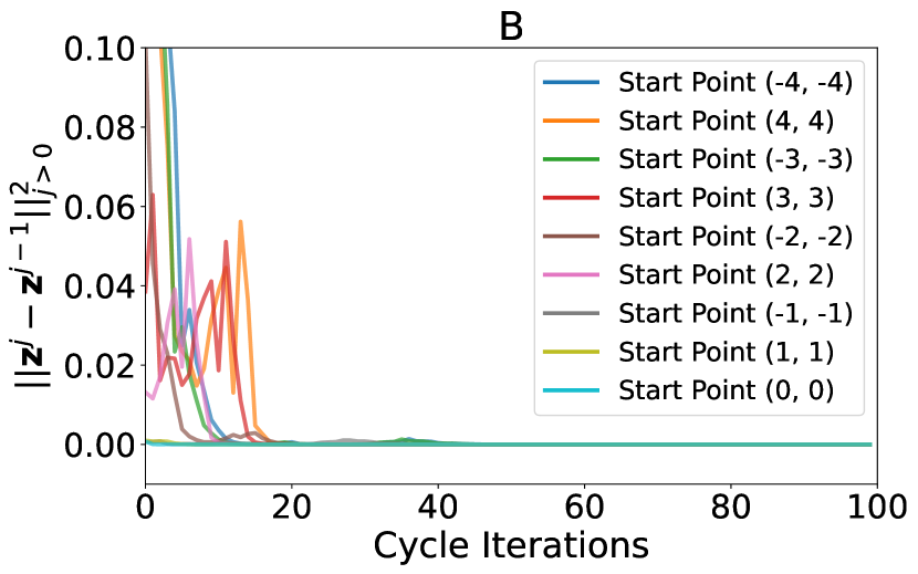
Figure 4: Figures demonstrate the relationship between latent inconsistency and the density of the latent variable. A shows the $||\bm{z}-\bm{z^{1}}||^{2}$ values of latent variables sampled from varying densities in LS. B shows the cycles of latent variables from different regions in LS, where Y-axis shows the difference between successive cycles, $||\bm{z^{j}}-\bm{z^{j-1}}||^{2}$, and X-axis shows the cycle iterations. In A, inconsistencies increase as the density in LS decrease. In B, convergence requires more cycle iterations as the density in LS decrease.

2.3 Two Critical Issues in LSBO

In this section, we discuss the two critical issues in the current LSBO.

2.3.1 Latent Inconsistency

Given a latent variable $\bm{z}$, we denote $\bm{z}^{1}=f^{\text{enc}}_{\phi}(f^{\text{dec}}_{\theta}(\bm{z}))$, $\bm{z}^{2}=f^{\text{enc}}_{\phi}(f^{\text{dec}}_{\theta}(\bm{z}^{1}))$, $\dots$, $\bm{z}^{M}=f^{\text{enc}}_{\phi}(f^{\text{dec}}_{\theta}(\bm{z}^{M-1}))$, where each step $f^{\text{enc}}_{\phi}(f^{\text{dec}}_{\theta}(\bm{z}^{j})),j\in[M]$ is referred as a cycle and the $M$ denotes the number of cycles. For a latent variable $\bm{z}\in{\mathcal{Z}}$, we formally say that it is latent consistent if $\bm{z}=\bm{z}^{M}$ when $M\to\infty$ and latent inconsistent otherwise. Note that, for a latent variable $\bm{z}$ to be consistent, it has to be converged to a single point in the LS. For latent inconsistent points, we consider the limiting distribution after a sufficient number of cycles. For a sufficiently large $B$, the limiting distribution of a latent variable $\bm{z}$ is defined as $\left\{\bm{z}^{j}\right\}_{j=B}^{M},M\to\infty$. Algorithm 1 describes how to find the limiting point/distribution by using the decoder and the encoder of a trained VAE.

When analyzing the latent space, it is observed that the proportion of consistent and inconsistent points, as well as the convergence speed, vary depending on the density of training instances. In a VAE, it is common to set the prior distribution as a standard normal distribution $N(\bm{0},I)$, resulting in high density near the origin $\bm{0}$, which decreases as we move away from the origin. Figure 4(A) illustrates the change in latent inconsistency (measured as $||\bm{z}-\bm{z}^{1}||^{2}$) with density in $N(\bm{0},I)$. It is evident that the issue of latent inconsistency is more pronounced in low-density regions. Additionally, Fig. 4(B) demonstrates the convergence properties of latent variables in different locations, revealing that latent variables in low-density regions converge slowly.

The important point to note is that the LSBO does not function as intended in regions with latent inconsistencies. In the LSBO process, a new latent variable $\bm{z}_{\rm new}$ is selected based on the AF of a BO algorithm. It is then decoded to $\bm{x}_{\rm new}$ and its corresponding BB function value $f^{\rm BB}(\bm{x}_{\rm new})$ is obtained. The new information is incorporated into the input dataset, which is then used to retrain both the VAE and the surrogate model. By retraining the models, the new knowledge is effectively integrated into the VAE and the surrogate model. However, a contradiction arises when $\bm{z}_{\rm new}$ is latent inconsistent. Specifically, during the update of the surrogate model, the BO algorithm queries the BB function value at $\bm{z}_{\rm new}$, but actually obtains the value corresponding to $\bm{z}_{\rm new}^{1}=f^{\rm enc}{\phi}(f^{\rm dec}{\theta}(\bm{z}_{\rm new}))$. This means that the surrogate model in the LS cannot be updated as intended. Figure 5(B) illustrates the changes in AF values with the degree of latent inconsistency $||\bm{z}-\bm{z}^{1}||^{2}$ when using the well-known AF called UCB in LSBO. It is evident that significant differences exist in the AF values within the regions of latent inconsistency. Consequently, even when the BO algorithm queries points with high AF values, it may end up querying points with low AF values.

Namely, LSBO does not work well in latent inconsistent regions, meaning that we must focus on latent consistent regions in LSBO. In the next section, we propose the LCA-AF as a new type of AF for LSBO. By utilizing LCA-AF, it becomes possible to focus the search on the regions of latent consistency in the LS.

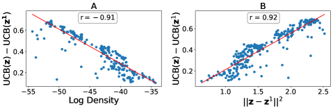
Figure 5: AF values, and squared differences of $\bm{z}$ and $\bm{z}^{1}$ using 32-dimensional LS of VAE with Transformer Encoder and Transformer Decoder trained on a database of chemical compounds, with UCB as AF. A shows the differences in the AF values against the density of $\bm{z}$, B shows the differences in the AF values against squared distances of $\bm{z}$ and $\bm{z}^{1}$. Results indicates high $\text{UCB}(\bm{z})-\text{UCB}(\bm{z}^{1})$ in low-density regions, and high correlation between $\text{UCB}(\bm{z})-\text{UCB}(\bm{z}^{1})$ and $||\bm{z}-\bm{z}^{1}||^{2}$.

2.3.2 Narrow Latent Consistent Regions

Although LSBO works well in the narrow latent consistent region as shown in Fig. 3(B), it fails to cover a wide range of LS effectively. Fig. 4 demonstrates that high-density regions are likely to be latent consistent, while low-density regions are likely to be latent inconsistent. Therefore, a search strategy that solely focuses on latent consistent regions cannot explore low-density regions. One key aspect of BO is the consideration of the exploration-exploitation trade-off. Exploitation mainly happens in high-density regions where known instances exist, while exploration typically occurs in low-density regions where no existing instances are found. This means that when a search strategy solely concentrates on the latent consistent region, it implies only exploitation is carried out, and exploration of unseen low-density regions is neglected.

Actually, as shown in Figs. 3(A) and (B), latent variables in sparsely populated regions often move towards densely populated regions near the origin. This means that even when we prioritize exploration, we are actually engaging in exploitation. In other words, the LSBO may end up exploring regions that have already been exploited, completely missing out on the opportunity to explore new and unexplored regions of interest. Unfortunately, as long as such restricted search strategy is used, it becomes challenging to discover entirely new instances such as de novo chemical compounds. In the following section, we introduce the LCA-VAE as a new method for retraining VAEs. By utilizing this retraining method, we can expand the latent consistent regions in the LS, which in turn widens the search space for the LSBO and enables exploration of previously unseen promising regions. When comparing the latent consistent regions in Figs. 3(A) and (B) with those obtained by LCA-VAE in Figs. 3(C) and (D), it is evident that the latter is wider, demonstrating the ability to explore even in low-density regions where there are no training instances available.

3 Proposed Method

In this section, we introduce our proposals: LCA-AF, LCA-VAE, and LCA-LSBO. These proposed methods help us to tackle the problem of latent inconsistencies, and the narrow consistent regions in the LS, improving the performance of LSBO algorithms.

3.1 LSBO with Consistent Points: LCA-AF

The idea behind the LCA-AF is to alleviate the disadvantage of latent inconsistencies by taking into account only the available consistent points. In LCA-AF, we modify AFs to use only consistent points in the LS for LSBO algorithms. After a sufficiently large number of cycles $B$, if we observe $\bm{z}^{B+1}-\bm{z}^{B}\approx\bm{z}^{B+2}-\bm{z}^{B+1}\approx$, …, $\approx\bm{z}^{M-1}-\bm{z}^{M-2}\approx\bm{z}^{M}-\bm{z}^{M-1}\approx\epsilon$, where $\epsilon$ is a constant taking values close to zero, we identify approximate convergence to a consistent point at $\bm{z}^{B}$. Since we are interested in the consistent points in LCA-AF, we can discard the latent variables obtained at the initial cycle iterations, before convergence is obtained. Therefore, given a latent variable $\bm{z}$, our interest lies in $\{f^{\textnormal{AF}}({\bm{z}}^{j})\}_{j\in[B,M]}$. The AF values are then computed by taking the mean of the AF values of $\{\bm{z}^{j}\}_{j\in[B,M]}$. We denote the resulting AF value as

$$\widehat{f^{\textnormal{LCA-AF}}({\bm{z}}^{j})}_{j\in[B,M]}=\frac{\displaystyle\sum_{j=B}^{M}f^{\textnormal{AF}}({\bm{z}}^{j})}{M-B}.$$ (2)

Given that convergence is observed after cycle iteration $B$, the convergence point $f^{\rm AF}({\bm{z}}^{M})$ can be approximated by $\widehat{f^{\textnormal{LCA-AF}}({\bm{z}}^{j})}_{j\in M\geq B}$.

We describe an LSBO algorithm that incorporates the LCA-AF in Algorithm 2. This algorithm considers the case where the VAE is retrained after new instance(s) are obtained by BO which uses the proposed AF demonstrated above. Selection by LCA-AF maintains consistency in LSBO, and therefore helps us to deal with the contradictory behavior of LSBO emerged from the latent inconsistencies, enabling LSBO to work as it is supposed to work.

Algorithm 2 LSBO with LCA-AF

1:Unlabeled instances: $\mathcal{U}=\{x_{i}\}_{i\in[\mathcal{U}]}$, Labeled instances: $\mathcal{L}=\{(x_{i},y_{i})\}_{i\in[\mathcal{L}]}$, $f^{\rm AF}(\bm{z})$, AF $f^{\textnormal{AF}}$, BB Function $f^{\textnormal{BB}}$, Experiment count $J$, Burn-in threshold $B$, VAE Encoder $f_{\phi}^{\textnormal{enc}}$ and VAE Decoder $f_{\theta}^{\textnormal{dec}}$

2:for $j=1$ to $J$ do

3:     Fit GP model using $\{(f_{\phi}^{\rm enc}(x_{i}),y_{i})\}_{i\in\mathcal{L}}$

4:     Find ${\bm{z}}\leftarrow\arg\max\widehat{f^{\textnormal{LCA-AF}}({\bm{z}}^{j})}_{j\in M\geq B}$

5:     Generate object: $\hat{x}^{*}=f^{\rm dec}_{\theta}(\bm{z})$

6:     Evaluate label: $y^{*}=f^{\rm BB}(\hat{x}^{*})$

7:     Update: $\mathcal{L}\leftarrow\mathcal{L}\cup(\hat{x}^{*},y^{*})$

8:     ReTrain $f_{\phi}^{\textnormal{enc}}$ and $f_{\theta}^{\textnormal{dec}}$ using $\{\{x_{i}\}_{i\in[\mathcal{U}]}\cup\{x_{i}\}_{i\in[\mathcal{L}]}\}$

9:end for

3.2 LCA-VAE

As discussed in §2.3, the availability of consistent points is limited, particularly in low-density regions of the LS, limiting exploration capabilities of BO. To tackle this problem and to enhance the exploration capabilities of LSBO, we introduce a novel VAE model called LCA-VAE. It is designed to improve latent consistencies specifically in these low-density regions and increase the number of consistent points in LS. This is achieved through the inclusion of the Latent Consistency Loss (LCL) in the VAE objective function. For a latent variable $\bm{\hat{z}}\in{\mathcal{Z}}$, the LCL is defined as

$${\rm LCL}(\bm{\hat{}}{z})=\sum_{j=1}^{M}||\bm{\hat{z}}-{\bm{\hat{z}}}^{j}||^{2},$$ (3)

which calculates the distance between the latent variable $\bm{\hat{z}}$ and its $M$ cycles that obtained after. Using the LCL, the objective function of the LCA-VAE is written as

$$J^{\rm LCA}_{\rm VAE}(\phi,\theta)=J_{\rm VAE}(\phi,\theta)-\gamma\mathbb{E}_{\bm{\hat{z}}\sim p_{\rm ref}(\bm{\hat{z}})}\left[{\rm LCL}(\bm{\hat{z}})\right],$$ (4)

where $\gamma>0$ is a hyperparameter to trade-off the balance between the two terms. In LCL, we use the latent variable $\bm{\hat{z}}$, which is sampled from a distribution which we call latent reference distribution, and denote as $p_{\rm ref}$. We use $\widehat{\rm hat}$ notation to denote the artificial instances from the latent reference distribution. We optimize the LCL of the $\bm{\hat{z}}$ sampled from $p_{\rm ref}$, which provides us versatility to shape the LS at the region of interest. We discuss strategies to select $p_{\rm ref}$ and their impact on LS in §3.2.1.

The implementation of the LCA-VAE is simple; we can optimize (the parameters of) encoder $f_{\phi}^{\rm enc}$ and decoder $f_{\theta}^{\rm dec}$ of the VAE using an empirical version of the objective function in (4), where an extra term

$$\frac{1}{\hat{N}*M}\sum_{i=1}^{\hat{N}}\sum_{j=1}^{M}\|\bm{\hat{z}_{i}}-\bm{\hat{z}}^{j}_{i}\|^{2}\simeq\mathbb{E}_{\bm{\hat{z}}\sim p_{\rm ref}(\bm{\hat{z}})}\left[{\rm LCL}(\bm{\hat{z}}),\right]$$ (5)

is subtracted (with multiplication with hyperparameter $\gamma$) from the empirical objective function of the standard VAE in (1). Here, $\bm{\hat{z}}_{i},i\in[\hat{N}],$ is a latent variable sampled from latent reference distribution $p_{\rm ref}$, and $\hat{N}$ is the number the sampled latent variables.

3.2.1 Latent Reference Distribution

In the LCA-VAE, the desired reference distribution, $p_{\rm ref}$, can be customized based on the target task. For our LSBO task, a common approach is to begin with a pretrained VAE and then refine it using newly acquired information through each step of BO. Consequently, we consider two types of reference distributions: one for the initial pretrained phase and another for the subsequent BO phase.

In the pretraining phase, our goal is to promote the latent consistency broadly throughout the LS. Therefore, we consider the reference distribution $p_{\rm ref}(\bm{z})$ such that it spans the entire support of the VAE’s latent variables’ prior distribution. Following this strategy, we adopt a spherical multivariate normal distribution for $p_{\rm ref}$, expressed as $N(\bm{\mu}_{\rm ref},\sigma_{\rm ref}^{2}I)$, where $\bm{\mu}_{\rm ref}\in{\mathcal{Z}}$ is the mean vector, and $\sigma_{\rm ref}>0$ is the standard deviation. If the prior distribution of a VAE is set as the standard normal distribution $N(\bm{0},I)$, we choose $\sigma_{\rm ref}$ to be larger than 1 to explore a wider range. In our numerical experiments in §4, we set $\sigma_{\rm ref}$ to 2. Figures 3(C) and (D) demonstrate the LS of LCA-VAE with this latent reference distribution. Unlike Figs.3(A) and (B), we observe an improvement in latent consistency (Fig. 3(C)), with an increased coverage of the LS in the expanded region of latent consistency (Fig. 3(D)).

In the BO phase, our goal is to ensure the latent consistency in the regions of interest indicated by the AFs of the LSBO algorithm. To achieve this, we use a reference distribution denoted as $p_{\rm ref}(\bm{z})$ which is adaptively determined based on the AF at each iteration of the BO process. Specifically, we set the $\bm{\mu}_{\rm ref}\leftarrow\arg\max\widehat{f^{\textnormal{LCA-AF}}({\bm{z}}^{j})}_{j\in[B,M]}$, meaning that we sample artificial points at the surrounding of the point with highest AF to improve latent consistency at that region. This approach can be thought of as an adaptive data augmentation in the LS, using AF values to update the VAE. By gradually expanding the search space in the LS and incorporating the promising regions indicated by the BO algorithm, the chance of discovering de novo instances located far from the training instances is enhanced.

3.3 LCA-LSBO

Combining LCA-AF and LCA-VAE, we propose LCA-LSBO for improved LSBO performance. LCA-LSBO utilizes the consistent points in LS through LCA-AF while increasing the number of consistent points in the LS and providing consistency in the region of interest through LCA-VAE. Algorithm 3 describes LCA-LSBO. Starting from the Cycle Pretrained LCA-VAE, we use the LCA-AF to pinpoint the highest value query point. Next, we set the latent reference distribution’s center $\bm{\mu}_{\rm ref}$ to that point, and set $\sigma_{\rm ref}<1$ to focus the $\hat{\bm{z}}$ in the close vicinity of the region where AF is maximized. We draw $\{\bm{\hat{z}}_{i}\}_{i\in[N^{*}]}$ using such $p_{\rm ref}$, and retrain the LCA-VAE model. Once we reach the retraining iteration limit, we obtain $\hat{\bm{x}}^{*}=f_{\theta}^{\rm dec}(\bm{\mu}_{\rm ref})$ and $y^{*}=f^{\rm BB}(\hat{\bm{x}}^{*})$, subsequently adding a new instance $(\bm{\mu}_{\rm ref},y^{*})$ to the labeled training set for the GP surrogate model in the LS.

Algorithm 3 Latent Consistency Aware-LSBO

1:Unlabeled instances: $\mathcal{U}=\{x_{i}\}_{i\in[\mathcal{U}]}$, Labeled instances: $\mathcal{L}=\{(x_{i},y_{i})\}_{i\in[\mathcal{L}]}$, $f^{\rm AF}(\bm{z})$ , AF $f^{\textnormal{AF}}$, BB Function $f^{\textnormal{BB}}$, Experiment count $J$, Burn-in threshold $B$, Standard Deviation of $p_{\rm ref}$: $\sigma_{\rm ref}$, Sample size of ${\hat{\bm{z}}}$: $N^{*}$

2:Train LCA-VAE with $p_{\rm ref}$ $\mathcal{N}(\bm{0},2*I)$

3:for $j=1$ to $J$ do

4:     Fit GP model using $\{(f_{\phi}^{\rm enc}(x_{i}),y_{i})\}_{i\in\mathcal{L}}$

5:     Find ${\bm{z}}\leftarrow\arg\max_{\bm{z}\in\mathcal{Z}}\widehat{f^{\textnormal{LCA-AF}}(\hat{\bm{z}}_{i})}_{i\in M\geq B}$ and set $\bm{\mu}_{\rm ref}\leftarrow$ $\bm{\hat{z}}_{M}$

6:     Generate object: $\hat{x}^{*}=f^{\rm dec}_{\theta}(\bm{z})$

7:     Evaluate label: $y^{*}=f^{\rm BB}(\hat{x}^{*})$

8:     Update: $\mathcal{L}\leftarrow\mathcal{L}\cup(\hat{x}^{*},y^{*})$

9:     Obtain samples $\{{\bm{\hat{z}_{i}}}\}_{i\in[N^{*}]}\sim p_{\rm ref}$

10:     ReTrain LCA-VAE using $\{\{\bm{x_{i}}\}_{i\in[\mathcal{U}]}\cup\{\bm{x_{i}}\}_{i\in[\mathcal{L}]}\}$ and $\{{\bm{\hat{z}_{i}}}\}_{i\in[N^{*}]}$

11:end for

4 Numerical Experiments

We considered two different LSBO tasks. One is MNIST digit generation, and the other is de novo chemical compound design.

4.1 MNIST Digit Generation

The generation of MNIST digits is generally considered as a too simple task. However, by introducing a subtle variation, we can transform it into a challenging problem that mirrors the task of de novo object design. We considered 10 distinct LSBO tasks. In each task, we trained a VAE on the MNIST dataset that excludes instances of one particular digit $D\in\{0,1,2,3,4,5,6,7,8,9\}$. Then, we considered the task of generating the excluded digit that the model has not been trained on. To mimic the BB function for each task, we trained a classifier to distinguish the target digit $D$ from the rest. The classifier assigns a probability to the target digit when given an image, and this probability serves as the score for the BB function. Namely, the objective of each task is to generate a novel image that maximizes the BB function. For example, in the 1st task with $D=0$, we trained a VAE using images of digits 1 to 9 in the MNIST dataset, and considered an LSBO task with the goal of generating an images that look 0. We performed the similar tasks also for the cases of $D=1,2,\ldots,9$ and evaluated the generated images of “unknown” digits produced by the proposed method and several baseline methods. These tasks mirror the requirements of de novo object design tasks, where the goal is to generate an object that is not part of the training instances. Through this modified approach to MNIST digit generation, we aim to demonstrate the versatility and adaptability of our methodology and limitations of other existing approaches.

We examined three versions of the proposed method. They are called LCA-AF, LCA-AF(RT), and LCA-LSBO. LCA-AF and LCA-AF(RT) refer to the LSBO method that uses the proposed LCA-AF as the AF in §3.1. In the former, we used a fixed VAE throughout the LSBO process, meaning that we did not retrain the VAE, In the latter, we retrained the VAE every time we obtained a new labeled instance. LCA-LSBO is a method that combines both the LCA-AF in §3.1 and the LCA-VAE in §3.2. The reason for considering not only the best-performing LCA-LSBO but also suboptimal LCA-AF and LCA-AF(RT) is to assess the impact of retraining the VAE and our two main proposals: focusing only on latent consistent points during BO and retraining with the LCA-VAE method. By isolating these components, we aim to gain a more detailed understanding of how each one contributes to the overall performance.

As baselines, we considered 9 methods: vanilla-VAE, vanilla-VAE(RT), predictor-VAE, predictor-VAE(RT), conditional-VAE, conditional-VAE(RT), weighted RT, and DML RT. The first two baselines: vanilla-VAE and vanilla-VAE(RT) refer to the standard LSBO methods using a vanilla VAE [1] without or with retraining option, respectively. The next two baselines predictor-VAE and predictor-VAE(RT) refer to the LSBO methods with predictor [1] without or with retraining option, respectively. The next two baselines conditional-VAE and conditional-VAE(RT) refer to the LSBO methods in which conditional VAEs are used [22] without or with retraining option, respectively. The next baseline weighted RT [14] is an LSBO method in which the instances are weighted according to the AF values when the VAE is retrained. The last baseline DML RT [16] is an LSBO method in which distance metric learned in the LS is incorporated when the VAE is retrained.

In all versions of the proposed method and baseline methods except conditional-VAE and conditional-VAE(RT), the dimension of the LSs were set to 2. Since conditional-VAE and conditional-VAE(RT) require additional latent dimension, the dimension of their LSs were set to 3. For other hyperparameters, the same values are used in all methods, and changing their values did not have a significant impact on the results (see App. A).

4.1.1 Results

We started by exploring baseline methods that do not incorporate retraining of the VAE with newly obtained instances during the BO process. For each method and task, we conducted BO for a total of 200 iterations. The results of these experiments are detailed in Table 1, where we provide generated samples. Interestingly, we observe that all the methods without retraining (including LCA-AF) completely failed to generate the unseen target digits. This observation highlights the concept we initially proposed regarding the mismatch between the objectives of the VAE and the BO. Specifically, the VAE is specifically devised and trained to generate instances that closely resemble their input instances, resulting in the inability to generate entirely new instances.

In the next set of experiments, we evaluated the performance when the VAE in the corresponding method is retrained with the new information obtained by BO. For each method, we retrained the VAE after new instance is obtained by BO. Table 2 shows the generated samples with the highest probability of being target digit. The results demonstrate that the performances were improved by retraining the VAE. We observe that vanilla-VAE(RT) is successful at two tasks (1,6), predictor-VAE(RT) is successful at three tasks (1,5,7), and conditional-VAE(RT) is successful at three tasks (0,6,9). Weighted RT improves upon vanilla-VAE(RT), while DML RT can identify the same digits as Weighted RT and provides a better performance for digit 2.

We observe that LCA-AF(RT) provides better performance compared to all the baselines: it can successfully generate or approximate the target digit in seven out of ten tasks (0,2,3,4,6,7,8). This suggests that focusing on latent consistent points via LCA-AF can significantly enhance the LSBO performance. Finally, LCA-LSBO exhibits superior performance compared among all the methods: it successfully accomplishes all the 10 tasks, demonstrating that combining LCA-AF and LCA-VAE provides improvement. This highlights the potential of our proposed method in effectively generating target objects thanks to its improved exploration capabilities in the LS.

Table 1: Performance of baseline methods that do not use retraining.

Digit	vanilla-VAE	predictor VAE	conditional-VAE	LCA-AF
0
1
2
3
4
5
6
7
8
9

Table 2: Each image represents the image with highest probability of being the target digit after every second retraining.

Digit	vanilla-VAE(RT)	predictor-VAE(RT)	conditional-VAE(RT)
0
1
2
3
4
5
6
7
8
9

Digit	weighted RT	DML RT	LCA-AF(RT)	LCA-LSBO
0
1
2
3
4
5
6
7
8
9

4.2 De Novo Chemical Design

In this experiment, we utilized the ZINC250K dataset [1] to train our VAE. Each chemical compound in this dataset is represented using the SELFIES format [23], as it provides superior validity properties over the more commonly used SMILES representation. We implement the Transformer LCA-VAE model with Transformer Encoder and Transformer Decoder, both of which use 8 heads, 6 layers, and a 32-dimensional LS.

Our objective in this experiment is to optimize the docking scores of molecules, aiming for the lowest possible score when docking to site18 of the KAT1 protein. Docking scores are computed using Schrödinger’s simulator [24]. To facilitate this, we first determine the 3D representation of the generated chemical compound utilizing Schrödinger’s LigPrep software. Subsequently, the Glide software, also by Schrödinger, is used to calculate docking scores.

Given the potential time consumption of docking score computation—ranging from a few minutes to half an hour depending on the complexity of the chemical compound—as well as the possibility of failure in creating the 3D structure of the molecule or docking the protein, we put significant emphasis on sample efficiency in our experiment. To establish a benchmark for our methodology, we randomly select 50, 000 chemical compounds from the ZINC database [25] and evaluate their docking scores, comparing these against the scores generated by our method over 500 iterations of the BO algorithm using Algorithm 3. We further impose a constraint that both generated chemical compounds and 50, 000 chemical compounds from ZINC database have molecular weights lower than 450 Da (Dalton), calculated by summing the weights of each atom in the molecule, respecting the Lipinski’s Rule of Five [26], which states that molecules with a molecular weight over 500 Da becomes harder to synthesize.

4.2.1 Results

We employ Algorithm 3 in conjunction with the Transformer LCA-VAE and execute 500 iterations of BO. The results of this experiment are depicted in Figure 6. Fig. 6(A) demonstrates the lowest docking score in each iteration of BO and the lowest docking score from 50, 000 instances from ZINC database, and Fig. 6(B) demonstrates the distribution of the docking scores of the molecules.

As shown in Fig. 6(A), our method succeeds in generating a de novo molecule with a docking score lower than 50, 000 instances from ZINC database, and it achieves this in fewer than 500 iterations. The molecule with the lowest docking score among the 50, 000 selected random from the ZINC database exhibits a docking score of $-8.8$. Our approach identifies molecules with docking scores as low as $-9.58$ within just 500 iterations. Some of the molecules that achieved docking scores lower than -8 are showcased in Figure 7. Besides, Table 3 shows the comparison of the Top 3 lowest docking scores obtained by 50, 000 molecules from ZINC database and our method, where our method provides better scores in each level. It shows that our method can explore many de novo chemical compounds of interest within limited number of BO iterations. Besides, Fig. 6(B) shows that docking score distribution of LCA-LSBO samples are shifted towards a lower value compared with the samples from ZINC database.

Given the significant time and financial investment required to conduct docking simulations using highly accurate simulators, it becomes imperative to have a model that exhibits high sample-efficiency and good exploration capabilities. As our experiments with the MNIST dataset have also demonstrated, our method exhibits promising sample-efficiency characteristics. Results underscore the importance of focusing on consistent points through LCA-AF, and employing LCA-VAE with LCA-AF in LSBO tasks.

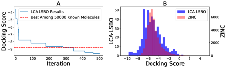
Figure 6: Comparison of LCA-LSBO and 50,000 samples from ZINC database. A shows BO results of Docking Score experiments and the lowest docking score obtained by 50,000 sample. Lower is better. LCA LSBO generates molecules with lower docking scores than 50,000 samples within 500 iterations. B shows distribution of docking scores, lower us better. This plot has two y-axes with different scales. Left y-axis of B demonstrates frequencies of LCA LSBO samples and right y-axis of B demonstrates frequencies of 50,000 ZINC samples. Distribution of samples from LCA LSBO are shifted towards lower values.

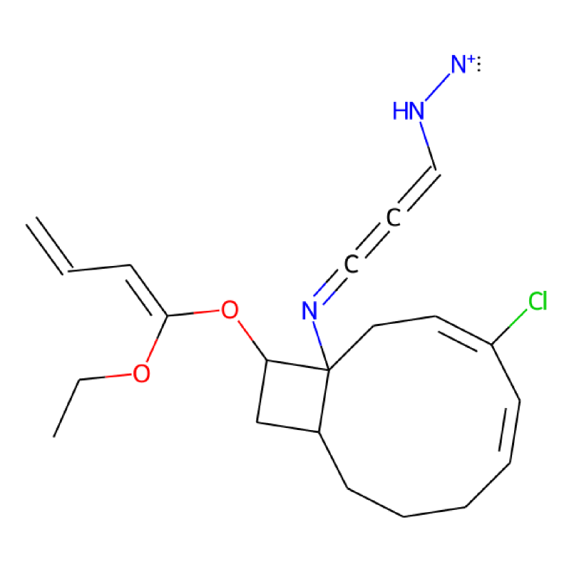
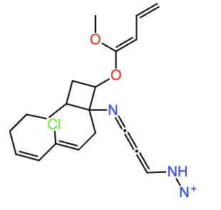
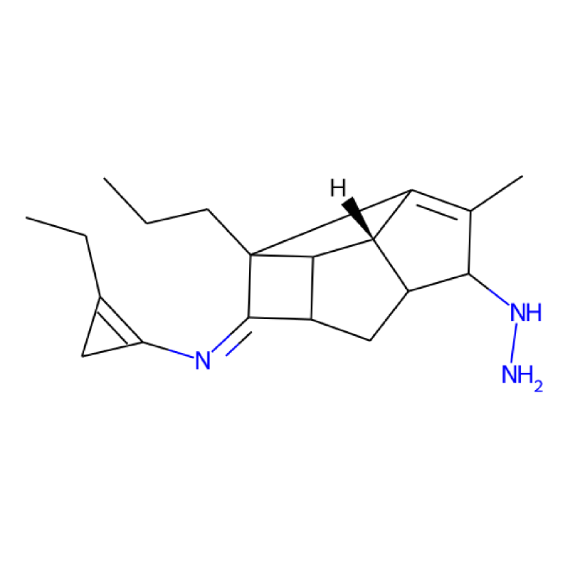
Figure 7: Example molecules with DS values lower than $-8$.

Table 3: Comparison of TOP 3 molecules with lowest docking scores.

Method	Sample Size	$\mathbf{1^{st}}$	$\mathbf{2^{nd}}$	$\mathbf{3^{rd}}$
ZINC Database	50,000	-8.80	-8.66	-8.51
Ours	500	-9.58	-9.54	-9.44

5 Conclusion

In conclusion, our research has focused on developing a novel approach for efficient LSBO in complex scenarios. Our experiments have demonstrated the promising characteristics of our method, showcasing its high sample-efficiency and effective exploration capabilities. The results obtained from our experiments with the MNIST dataset and docking scores have validated the effectiveness of our approach. The emphasis on consistent points through LCA-AF and the utilization of LCA-VAE in LSBO tasks have proven to be crucial factors in achieving optimal solutions. These findings highlight the potential of our LCA-LSBO approach for real-world applications, where the efficient use of resources is paramount.

Appendix A Impact of Cycle Count and $\gamma$

The selection of hyperparameters $M$ and $\gamma$ in LCL depends on VAE’s latent dimension. In 2-dimensional LS, a wide range of $\gamma$ values improves LSBO performance. However, in higher dimensions, setting $\gamma<1$ outperforms $\gamma>1$ due to increased LCL. When LCL is high and we set $\gamma>1$, it causes prioritization of latent consistency over representation learning and reconstruction capabilities. In our experiments with Transformer LCA-VAE, we set $\gamma=0.1$. The number of cycles in LCL has a similar impact to $\gamma$. While a single cycle suffices for 32-dimensional LS, multiple cycles in 2-dimensional LS enhance consistencies without affecting LSBO performance.

Declarations

• Funding This work was partially supported by MEXT KAKENHI (20H00601), JST CREST (JPMJCR21D3, JPMJCR21D3), JST Moonshot R&D (JPMJMS2033-05), JST AIP Acceleration Research (JPMJCR21U2), NEDO (JPNP18002, JPNP20006) and RIKEN Center for Advanced Intelligence Project.

• Conflicts of interest/Competing interests Not applicable.

• Ethics approval Not applicable.

• Consent to participate Not applicable.

• Consent for publication Not applicable.

• Availability of data and material Open-source datasets are used.

• Code availability Codes are available at github.com/onurboyar/lca-lsbo.

• Authors’ contributions Mr. Boyar contributed to the original research ideas, conducted the experiments, and wrote parts of the manuscript. Prof. Takeuchi supervised the research progress, contributed to the original research ideas, and wrote parts of the manuscript.

References

- \bibcommenthead
- Gómez-Bombarelli et al. [2018] Gómez-Bombarelli, R., Wei, J.N., Duvenaud, D., Hernández-Lobato, J.M., Sánchez-Lengeling, B., Sheberla, D., Aguilera-Iparraguirre, J., Hirzel, T.D., Adams, R.P., Aspuru-Guzik, A.: Automatic chemical design using a data-driven continuous representation of molecules. ACS Central Science 4(2), 268–276 (2018) https://doi.org/10.1021/acscentsci.7b00572
- Kingma and Welling [2014] Kingma, D.P., Welling, M.: Auto-encoding variational bayes. In: Bengio, Y., LeCun, Y. (eds.) 2nd International Conference on Learning Representations, ICLR 2014 (2014)
- Razavi et al. [2019] Razavi, A., Oord, A., Vinyals, O.: Generating diverse high-fidelity images with vq-vae-2. In: Wallach, H., Larochelle, H., Beygelzimer, A., Alché-Buc, F., Fox, E., Garnett, R. (eds.) Advances in Neural Information Processing Systems, vol. 32 (2019)
- Xu et al. [2018] Xu, H., Chen, W., Zhao, N., Li, Z., Bu, J., Li, Z., Liu, Y., Zhao, Y., Pei, D., Feng, Y., Chen, J., Wang, Z., Qiao, H.: Unsupervised anomaly detection via variational auto-encoder for seasonal kpis in web applications, pp. 187–196 (2018). https://doi.org/10.1145/3178876.3185996
- Im et al. [2017] Im, D.I., Ahn, S., Memisevic, R., Bengio, Y.: Denoising criterion for variational auto-encoding framework. Proceedings of the AAAI Conference on Artificial Intelligence 31(1) (2017) https://doi.org/10.1609/aaai.v31i1.10777
- Frazier [2018] Frazier, P.: A tutorial on bayesian optimization. ArXiv abs/1807.02811 (2018)
- Kandasamy et al. [2018] Kandasamy, K., Neiswanger, W., Schneider, J., Póczos, B., Xing, E.P.: Neural architecture search with bayesian optimisation and optimal transport. In: Proceedings of the 32nd International Conference on Neural Information Processing Systems (2018)
- Berthelot et al. [2022] Berthelot, D., Raffel, C., Roy, A., Goodfellow, I.: High-dimensional bayesian optimization with invariance (2022)
- Choudhary et al. [2022] Choudhary, K., DeCost, B., Chen, C., Jain, A., Tavazza, F., Cohn, R., WooPark, C., Choudhary, A., Agrawal, A., Billinge, S., Holm, E., Ong, S., Wolverton, C.: Recent advances and applications of deep learning methods in materials science. npj Comput Mater 8 (2022)
- Hie and Yang [2022] Hie, B.L., Yang, K.K.: Adaptive machine learning for protein engineering. Current Opinion in Structural Biology 72, 145–152 (2022) https://doi.org/10.1016/j.sbi.2021.11.002
- Richards and Groener [2022] Richards, R., Groener, A.: Conditional beta-vae for de novo molecular generation (2022) https://doi.org/10.26434/chemrxiv-2022-g3gvz
- Griffiths and Hernández-Lobato [2020] Griffiths, R.-R., Hernández-Lobato, J.M.: Constrained bayesian optimization for automatic chemical design using variational autoencoders. Chem. Sci. 11, 577–586 (2020) https://doi.org/10.1039/C9SC04026A
- Siivola et al. [2021] Siivola, E., Paleyes, A., González, J., Vehtari, A.: Good practices for bayesian optimization of high dimensional structured spaces. Applied AI Letters 2 (2021) https://doi.org/10.1002/ail2.24
- Tripp et al. [2020] Tripp, A., Daxberger, E., Hernández-Lobato, J.: Sample-efficient optimization in the latent space of deep generative models via weighted retraining. In: Advances in Neural Information Processing Systems (2020)
- Maus et al. [2022] Maus, N., Jones, H., Moore, J., Kusner, M.J., Bradshaw, J., Gardner, J.: Local latent space bayesian optimization over structured inputs. Advances in Neural Information Processing Systems 35, 34505–34518 (2022)
- Grosnit et al. [2021] Grosnit, A., Tutunov, R., Maraval, A.M., Griffiths, R.-R., Cowen-Rivers, A.I., Yang, L., Zhu, L., Lyu, W., Chen, Z., Wang, J., Peters, J., Bou-Ammar, H.: High-dimensional bayesian optimisation with variational autoencoders and deep metric learning. ArXiv abs/2106.03609 (2021)
- Jha et al. [2018] Jha, A.H., Anand, S., Singh, M., Veeravasarapu, V.R.: Disentangling factors of variation with cycle-consistent variational auto-encoders. In: Proceedings of the European Conference on Computer Vision (ECCV), pp. 805–820 (2018)
- Moriconi et al. [2020] Moriconi, R., Deisenroth, M.P., Sesh Kumar, K.: High-dimensional bayesian optimization using low-dimensional feature spaces. Machine Learning (2020)
- Fawzi et al. [2016] Fawzi, A., Samulowitz, H., Turaga, D., Frossard, P.: Adaptive data augmentation for image classification. In: 2016 IEEE International Conference on Image Processing (ICIP), pp. 3688–3692 (2016)
- Higgins et al. [2016] Higgins, I., Matthey, L., Pal, A., Burgess, C.P., Glorot, X., Botvinick, M.M., Mohamed, S., Lerchner, A.: beta-vae: Learning basic visual concepts with a constrained variational framework. In: International Conference on Learning Representations (2016)
- Deng [2012] Deng, L.: The mnist database of handwritten digit images for machine learning research. IEEE Signal Processing Magazine 29(6), 141–142 (2012)
- Lim et al. [2018] Lim, J., Ryu, S., Kim, J., Kim, W.: Molecular generative model based on conditional variational autoencoder for de novo molecular design. Journal of Cheminformatics 10 (2018) https://doi.org/10.1186/s13321-018-0286-7
- Krenn et al. [2020] Krenn, M., Häse, F., Nigam, A., Friederich, P., Aspuru-Guzik, A.: Self-referencing embedded strings (selfies): A 100% robust molecular string representation. Machine Learning: Science and Technology 1(4), 045024 (2020) https://doi.org/10.1088/2632-2153/aba947
- Schrödinger [2023] Schrödinger Suite. Computer Software, LLC, New York, NY. Release 2023-2 (2023)
- Irwin et al. [2020] Irwin, J.J., Tang, K.G., Young, J., Dandarchuluun, C., Wong, B.R., Khurelbaatar, M., Moroz, Y.S., Mayfield, J., Sayle, R.A.: Zinc20—a free ultralarge-scale chemical database for ligand discovery. Journal of chemical information and modeling 60(12), 6065–6073 (2020)
- Lipinski et al. [1997] Lipinski, C.A., Lombardo, F., Dominy, B.W., Feeney, P.J.: Experimental and computational approaches to estimate solubility and permeability in drug discovery and development settings. Advanced drug delivery reviews 23(1-3), 3–25 (1997)